On fractional elliptic equations
in Lipschitz sets and epigraphs:
regularity, monotonicity and rigidity results

Abstract.

We consider a nonlocal equation set in an unbounded domain with the epigraph property. We prove symmetry, monotonicity and rigidity results. In particular, we deal with halfspaces, coercive epigraphs and epigraphs that are flat at infinity.

These results can be seen as the nonlocal counterpart of the celebrated article [5].

1. introduction

The study of monotonicity and rigidity of solutions to semilinear elliptic equations of fractional order in the whole space $\mathbb{R}^{N}$ or in smooth bounded sets $\Omega$ has attracted considerable attention in the last years, see e.g. [3, 8, 9, 10, 11, 15, 19, 20, 28, 29, 43]. In striking contrast, if $\Omega$ is unbounded, but different from the whole space, very few results are available, all concerning the particular case of the half-space $\Omega=\mathbb{R}^{N}_{+}$, see [24, 35], or the one of exterior sets, see [34, 33, 44]. The main purpose of this paper is the study of the qualitative properties of bounded solutions to

(1.1) $$\begin{cases}(-\Delta)^{s}u=f(u)&\text{in $\Omega$},\\ u>0&\text{in $\Omega$},\\ u=0&\text{in $\mathbb{R}^{N}\setminus\Omega$},\end{cases}$$

where $\Omega$ is assumed to be the epigraph of a continuous function $\varphi:\mathbb{R}^{N-1}\to\mathbb{R}$, i.e. we suppose that

(1.2) $$\Omega:=\left\{x\in\mathbb{R}^{N}:x_{N}>\varphi(x^{\prime})\right\}\,,\qquad{\mbox{ with }}x^{\prime}=(x_{1},\dots,x_{N-1})\in\mathbb{R}^{N-1}.$$

Notice that the half-space $\mathbb{R}^{N}_{+}$ falls within this definition with $\varphi\equiv 0$.

In (1.1), $(-\Delta)^{s}$ with $s\in(0,1)$ denotes the fractional Laplacian, which can be defined as the operator acting on sufficiently smooth functions as

$$\begin{split}(-\Delta)^{s}u(x)&:=c_{N,s}\,PV\int_{\mathbb{R}^{N}}\frac{u(x)-u(y)}{|x-y|^{N+2s}}\,dy\\ &=c_{N,s}\lim_{\varepsilon\to 0^{+}}\int_{\mathbb{R}^{N}\setminus B_{\varepsilon}(x)}\frac{u(x)-u(y)}{|x-y|^{N+2s}}\,dy,\end{split}$$

where $c_{N,s}>0$ is a normalizing constant (which plays no major role in the present paper and which will be often omitted for simplicity), and $PV$ stays for “principal value”.

We will consider different assumptions on $\varphi$, obtaining different monotonicity and rigidity properties accordingly.

The nonlinearity $f$ in (1.1) belongs to a reasonably wide class of functions, including for instance those of bistable-type (a precise definition will follow shortly). Under these assumptions, the main results of this paper are:

• boundary regularity, monotonicity and further qualitative properties for solutions to (1.1) in globally Lipschitz epigraphs;

• monotonicity for solutions to (1.1) in coercive epigraphs;

• $1$-dimensional symmetry in the half-space;

• rigidity for overdetermined problems in epigraphs that are sufficiently “flat at infinity”.

Similar results in the classical case $s=1$ were obtained in the seminal paper [5]. Here, dealing with a nonlocal framework, a careful analysis is needed to overcome the lack of explicit barriers and several ad-hoc arguments will be exploited to replace the study of the point-wise behavior of the solution with a global study of the geometry of the problem.

As additional statements, we also derive a very general maximum principle (tailor-made for non-decaying solutions in possibly unbounded domains), a general version of the sliding method for the fractional Laplacian, and a boundary regularity result for solutions of fractional boundary value problems in sets satisfying an exterior cone condition.

Before proceeding with the statement of our results, we clarify that with the terminology solution in this paper we always mean classical solution.

As a matter of fact, without extra effort, the same results would apply to bounded viscosity solutions of (1.1): indeed, since we will assume that the nonlinearity $f$ is locally Lipschitz continuous, the regularity theory for viscosity solutions (developed in [13, 14]) implies that viscosity and classical solutions coincide in our setting (see [35, Remark 2.3] for a detailed explanation).

In addition, we mention that distributional (i.e. very weak) solutions or weak solutions (as defined e.g. in [24, 44]) could be considered as well with minor changes.

For the reader’s convenience, we will recall the definition of classical and viscosity solution at the end of the introduction.

In the next subsections, we describe in details the results obtained. In all the forthcoming statements, the fractional parameter $s$ will always be a fixed value in the interval $(0,1)$.

1.1. Boundary value problems in globally Lipschitz epigraphs

In this subsection we consider the case in which the domain $\Omega$ of (1.1) is a globally Lipschitz epigraph. Namely, we suppose that the function $\varphi$ in (1.2) is globally Lipschitz continuous, with Lipschitz constant $K$.

On the nonlinearity $f$, we suppose that:

• $f$ is locally Lipschitz continuous in $\mathbb{R}$, and there exists $\mu>0$ such that $f(t)>0$ for any $t\in(0,\mu)$, and $f(t)\leqslant 0$ for any $t\geqslant\mu$;

• there exist ${t_{0}}\in(0,\mu)$, and $\delta_{0}>0$ such that $f(t)\geqslant\delta_{0}\,t$ for any $t\in[0,{t_{0}}]$;

• there exists ${t_{1}}\in({t_{0}},\mu)$ such that $f$ is non-increasing in $({t_{1}},\mu)$.

As prototype example, we may think at $f(t)=t-t^{3}$, which yields the fractional Allen-Cahn equation, that is a widely studied model in phase transitions in media with long-range particle interactions, see e.g. [39].

The first of our main results is the natural counterpart of Theorems 1.1 and 1.2 in [5].

Theorem 1.1.

Let $\Omega$ be a globally Lipschitz epigraph. Let $f$ satisfy assumptions ($f1$)-($f3$), and let $u$ be a bounded solution to (1.1). Then:

• $u<\mu$ in $\Omega$.

• As ${\rm dist}(x,\partial\Omega)\to+\infty$, we have that $u(x)\to\mu$ uniformly in $\Omega$.

• There exist $C,\bar{\rho},h_{1}>0$ such that

  $$u(x^{\prime},x_{N})\geqslant C(x_{N}-\varphi(x^{\prime}))^{\bar{\rho}}\qquad\text{if $x_{N}-\varphi(x^{\prime})<h_{1}$}.$$

• $u$ is globally $\alpha$-Hölder continuous in $\mathbb{R}^{N}$, for some $\alpha\in(0,s)$.

• $u$ is the unique bounded solution to (1.1).

• If $(a_{1},\dots,a_{N-1})$ is such that

  $$\sum_{i}a_{i}^{2}<K^{-2},$$

  then

  $$\partial_{x_{N}}u+\sum_{i}a_{i}\partial_{x_{i}}u>0\qquad\text{in $\Omega$}.$$

  In particular, $u$ is monotone increasing in $x_{N}$.

We stress that, since $\Omega$ is merely a Lipschitz set and the exterior sphere condition is not necessarily satisfied along $\partial\Omega$, the Hölder continuity of the solution does not follow by previous contributions (see Subsection 1.4 for more details). Both the exponents $\bar{\rho}$ and $\alpha$ appearing in the theorem are determined by the choice of $\varphi$. To be more precise, we note that a globally Lipschitz epigraph satisfy both a uniform exterior cone condition with angle $\theta_{1}$ and a uniform interior cone condition with angle $\theta_{2}$ (see Subsection 1.4 for a precise definition of the exterior cone condition); then, as it will be clear from the proofs, the exponent $\alpha$ depends on $\theta_{1}$, while the index $\bar{\rho}$ depends on $\theta_{2}$.

Regarding point ($vi$) in the theorem, it establishes that $u$ is monotone increasing in any direction $\tau$ such that there exists an orthonormal basis $y_{1},\dots,y_{N}$ of $\mathbb{R}^{N}$ with $y_{N}=\tau$, and in the new coordinates $\Omega$ is still the epigraph of a globally Lipschitz function $\psi=\psi(y_{1},\dots,y_{N-1})$. Thus, in the particular case $\varphi\equiv 0$, i.e. when $\Omega=\mathbb{R}^{N}_{+}$ is a half-space, we deduce monotonicity and $1$-dimensional symmetry of the solutions.

Corollary 1.2.

Let $\Omega=\mathbb{R}^{N}_{+}$, and let $f$ satisfy ($f1$)-($f3$), and let $u$ be a bounded solution to (1.1). Then $u$ depends only on $x_{N}$, and

$$\partial_{x_{N}}u>0\qquad\text{in $\Omega$}.$$

Previous results regarding monotonicity of solutions to nonlocal equations in half-spaces can be found in [25, 35] (see also [40] for results in the whole of $\mathbb{R}^{N}$), where the authors dealt with non-decreasing nonlinearities $f$ satisfying $f(0)\geqslant 0$.

We also refer to [2] (which appeared after the present paper was submitted), where the authors proved that any bounded, non-negative and non-trivial solution to (1.1) with $f$ of class $\mathcal{C}^{1}$ is montone increasing.

In all the articles [2, 25, 35] the monotonicity is used to derive non-existence results for non-decreasing nonlinearities $f$, which is a complementary situation with respect to the one considered here.

The $1$-dimensional symmetry in the half-space, as addressed in Corollary 1.2, was, up to now, open.

Coming back to the monotonicity of the solutions, we emphasize that the main result in [2] allows to treat also the case $f(0)<0$. This marks a relevant difference with the local setting $s=1$, since in case $f(0)<0$ non-negative solutions of local equations are not necessarily monotone, and only partial results are available (we refer the interested reader to [4, 16, 18, 26, 27]).

The proof of Theorem 1.1 is given in Section 4, and relies on some classical ideas of [5] – nevertheless, all the intermediate steps present several substantial difficulties of purely nonlocal nature. As a matter of fact, in [5] the authors often construct more or less explicit local barriers, and exploit local properties of functions whose Laplacian has a strict sign. On the other hand, the construction of a barrier function is much harder when dealing with integro-differential operators, since such barrier has to be defined in the all space $\mathbb{R}^{N}$, and has to satisfy a boundary condition on the complement of a certain set $D$ (and not only on $\partial D$). Moreover, local properties of functions cannot be inferred by the only knowledge of the fractional Laplacian in some neighbourhood and any modification of the function “far away” affects the values of its fractional Laplacian at a point. These are just two sources of new obstructions which we shall overcome; we refer to the comments and the remarks written throughout the paper for further details.

1.2. Monotonicity of solutions in coercive epigraphs

In this subsection, we deal with the case in which the domain $\Omega$ of (1.1) is a coercive epigraph, namely, we suppose that the function $\varphi:\mathbb{R}^{N-1}\to\mathbb{R}$ in (1.2) is continuous and satisfies

$$\lim_{|x|^{\prime}\to+\infty}\varphi(x^{\prime})=+\infty.$$

In this setting, we have the following result:

Theorem 1.3.

Let $\Omega$ be a coercive epigraph, and let $u$ be a solution (not necessarily bounded) to

$$\begin{cases}(-\Delta)^{s}u=f(x,u)&\text{in $\Omega$},\\ u>0&\text{in $\Omega$},\\ u=0&\text{in $\mathbb{R}^{N}\setminus\Omega$},\end{cases}$$

with $f(x,t)$ continuous in $\overline{\Omega}\times\mathbb{R}$, non-decreasing in $x_{N}$, and locally Lipschitz continuous in $t$, locally uniformly in $x$, in the following sense: for any $M>0$ and any compact set $K\subset\overline{\Omega}$, there exists $C>0$ such that

$$\sup_{x\in K}\frac{|f(x,t)-f(x,\tau)|}{|t-\tau|}\leqslant C\qquad{\mbox{ for any }}t,\tau\in[-M,M].$$

Then $u$ is monotone increasing in $x_{N}$.

This result is the natural counterpart of [5, Theorem 1.3], which in turn is a refinement of [23, Proposition II.1]. Its proof rests on the moving planes method for the fractional Laplacian.

1.3. Overdetermined problems for the fractional Laplacian in epigraphs.

In this subsection, we consider the overdetermined setting in which both Dirichlet and Neumann conditions are prescribed in problem (1.1). Differently from the classical case, the Dirichlet condition needs to be set in the complement of the domain (and not along its boundary) and the Neumann assumptions takes into account (in a suitable sense) normal derivatives of fractional order.

For this, given an open set $\Omega$ with $\mathcal{C}^{2}$ boundary, we denote by $\nu(x_{0})$ the inner unit normal vector at $x_{0}\in\partial\Omega$. For any $u\in\mathcal{C}^{0,s}(\mathbb{R}^{N})$ and $x_{0}\in\partial\Omega$, we consider the outer normal $s$-derivative of $u$ in $x_{0}$, defined as

(1.3) $$(\partial_{\nu})_{s}u(x_{0}):=-\lim_{t\to 0^{+}}\frac{u(x_{0}+t\nu(x_{0}))-u(x_{0})}{t^{s}}.$$

The boundary regularity theory for fractional Laplacian, developed in [32, 31, 38, 37], ensures that, for a solution $u$ to (1.1) with $\Omega$ of class $\mathcal{C}^{2}$, the quantity $(\partial_{\nu})_{s}u$ is well defined. Natural Hopf’s Lemmas were then proved in [24, Proposition 3.3] and [30, Lemma 1.2], and constituted the base point in the study of overdetermined problems for the fractional Laplacian, see [17, 24, 30, 44, 34].

In this paper we consider overdetermined problems of the type

(1.4) $$\begin{cases}(-\Delta)^{s}u=f(u)&\text{in $\Omega$},\\ u>0&\text{in $\Omega$},\\ u=0&\text{in $\mathbb{R}^{N}\setminus\Omega$},\\ (\partial_{\nu})_{s}u=const.&\text{on $\partial\Omega$}.\end{cases}$$

We will suppose that $\Omega$ is the epigraph of a $\mathcal{C}^{2}$ and globally Lipschitz function $\varphi:\mathbb{R}^{N-1}\to\mathbb{R}$, satisfying the following additional assumption:

(1.5) $$\text{for any $\tau\in\mathbb{R}^{N-1}$, uniformly in $x^{\prime}$, }\lim_{|x^{\prime}|\to+\infty}(\varphi(x^{\prime}+\tau)-\varphi(x^{\prime}))=0.$$

This condition, firstly proposed in [5], can be seen as a flatness condition of $\partial\Omega$ at infinity.

We can extend [5, Theorem 7.1] in the nonlocal setting.

Theorem 1.4.

Let $\Omega$ be the epigraph of a $\mathcal{C}^{2}$ and globally Lipschitz function $\varphi:\mathbb{R}^{N-1}\to\mathbb{R}$, satisfying (1.5). Let $f$ satisfy ($f1$)-($f3$), and let us suppose that (1.4) has a bounded solution $u$. Then $\Omega$ is a half-space $\{x_{N}>const.\}$, and $u$ depends only on $x_{N}$ and is monotone increasing in $x_{N}$.

Theorem 1.4 is proved in Section 6.

1.4. Boundary regularity in domains satisfying an exterior cone condition

In this subsection, we obtain general boundary regularity results for solutions to

(1.6) $$\begin{cases}(-\Delta)^{s}u=g(x)&\text{in $\Omega$},\\ u=0&\text{in $\mathbb{R}^{N}\setminus\Omega$}.\end{cases}$$

In this setting, we will not restrict to the case in which $\Omega$ is an epigraph, but we will assume instead that $\Omega$ satisfies an exterior cone condition with some uniform opening $\theta\in(0,\pi)$. More precisely, for a given direction $e\in\mathbb{S}^{N-1}$ and a given angle $\theta\in(0,\pi)$, we denote by $\Sigma_{e,\theta}$ the open, rotationally symmetric cone of axis $e$ and opening $\theta$ (that is the set of all vectors $v\in\mathbb{R}^{n}$ that form with $e$ an angle less than $\theta$). We suppose that there exists $\theta\in(0,\pi)$ such that: if $x\in\partial\Omega$, then for a direction $e\in\mathbb{S}^{N-1}$ the cone $x+\Sigma_{e,\theta}$ is exterior to $\Omega$ and tangent to $\Omega$ in $x$.

We point out that in this definition the opening $\theta$ is the same for all the points of $\partial\Omega$, while the direction $e$ can change. We also observe that globally Lipschitz epigraphs $\{x_{N}>\varphi(x^{\prime})\}$ enjoy the uniform exterior cone condition, with $\theta$ depending only on the Lipschitz constant of $\varphi$.

The boundary regularity of solutions to boundary value problems driven by integro-differential operators has been object of several contributions [7, 32, 31, 36, 38, 37]. As far as we know, for boundary value problems of type (1.6) the minimal assumption on $\Omega$ was considered in [38, Proposition 1.1], where the authors supposed that $\Omega$ is a bounded Lipschitz domain satisfying a uniform exterior ball condition. The following theorem weaken this assumption, establishing the global Hölder continuity of bounded solutions to (1.6) when $\Omega$ satisfies a uniform exterior cone condition.

Theorem 1.5.

Let $\Omega$ be a possibly unbounded open set of $\mathbb{R}^{N}$, satisfying the uniform exterior cone condition with opening $\theta\in(0,\pi/2)$. Let $u\in L^{\infty}(\mathbb{R}^{N})$ be a solution to (1.6), with $g\in L^{\infty}(\Omega)$.

Then, there exist $\alpha\in(0,s)$ and $C>0$, both depending only on $\theta$, $s$ and $N$, such that $u\in\mathcal{C}^{0,\alpha}(\mathbb{R}^{N})$, and

(1.7) $$\|u\|_{\mathcal{C}^{0,\alpha}(\mathbb{R}^{N})}\leqslant C\left[\left(1+\|u\|_{L^{\infty}(\mathbb{R}^{N})}\right)\left(1+\|g\|_{L^{\infty}(\Omega)}^{\frac{\alpha}{2s-2\alpha}}\right)+\|g\|_{L^{\infty}(\Omega)}\right].$$

Also, for any $s\in(0,1)$, the map $\theta\mapsto\alpha(\theta,s)$ is monotone non-decreasing.

Remark 1.6.

We stress that it is not even necessary to suppose the Lipschitz regularity of $\Omega$.

If $\theta\geqslant\pi/2$, then the uniform exterior cone condition yields a uniform exterior sphere condition, and hence by [38, Proposition 1.1] solutions to fractional boundary value problems in $\Omega$ are already known to be of class $\mathcal{C}^{0,s}(\mathbb{R}^{N})$. This is why we only consider $\theta\in(0,\pi/2)$ in Theorem 1.5.

Remark 1.7.

The proof of Theorem 1.5 is based upon the construction of a wall of barriers, whose definition uses essentially the existence of homogeneous solutions to non-local problems in cones, contained in [1]. The homogeneity exponent appearing in this construction coincides precisely with the regularity index $\alpha$, and in particular the monotonicity of $\alpha$ in the angle $\theta$ follows from Lemma 3.3 in [1] (see Section 3, and in particular Remark 3.3, for more details).

For our purposes, the importance of (1.7) is to provide uniform convergence of sequences of solutions under very reasonable assumptions. Namely, let us consider a sequence $\{u_{n}\}$ of solutions to

$$\begin{cases}(-\Delta)^{s}u_{n}=g_{n}&\text{in $\Omega_{n}$},\\ u_{n}=0&\text{in $\mathbb{R}^{N}\setminus\Omega_{n}$},\end{cases}$$

with $\{u_{n}\}$ and $\{g_{n}\}$ uniformly bounded in $L^{\infty}(\mathbb{R}^{N})$ and $L^{\infty}(\Omega_{n})$, respectively. Then Theorem 1.5 implies that $u_{n}\to u_{\infty}$ locally uniformly in $\mathbb{R}^{N}$, up to a subsequence.

The proof of Theorem 1.5 is the object of Section 3.

1.5. Some useful results of independent interest

We conclude the introduction stating some general results that are auxiliary to the proof of the main theorems and which we think are also of independent interest.

In proving Theorem 1.1, a crucial tool will be a maximum principle in unbounded domain for the fractional Laplacian. This is the fractional counterpart of [5, Theorem 2.1], and we stress that while in the local case the domain $D$ is supposed to be connected, this is not necessary in the nonlocal setting.

Theorem 1.8.

Let $D$ be an open set in $\mathbb{R}^{N}$, possibly unbounded and disconnected. Suppose that $\overline{D}$ is disjoint from the closure of an infinite open connected cone. Let $z\in\mathcal{C}(\mathbb{R}^{N})$ bounded above, and satisfying in viscosity sense

(1.8) $$\begin{cases}(-\Delta)^{s}z-c(x)z\leqslant 0&\text{in $D$},\\ z\leqslant 0&\text{in $\mathbb{R}^{N}\setminus D$},\end{cases}$$

for some $c\in L^{\infty}(D)$, $c\leqslant 0$ a.e. in $D$, with $cz\in\mathcal{C}(D)$. Then $z\leqslant 0$ in $D$.

We observe that Theorem 1.8 here improves [21, Theorem 2.4], where a similar result was proved when $D$ was a half-space.

We shall also need the following version of the sliding method for the fractional Laplacian.

Theorem 1.9.

Let $\Omega$ be a bounded open subset of $\mathbb{R}^{N}$, convex in the direction $e_{N}=(0^{\prime},1)$. Let $w$ be a solution of

$$\begin{cases}(-\Delta)^{s}w=g(x,w)&\text{in $\Omega$},\\ w=\varphi&\text{in $\mathbb{R}^{N}\setminus\Omega$},\end{cases}$$

with $g(x,t)$ continuous in $\overline{\Omega}\times\mathbb{R}$, non-decreasing in $x_{N}$, and locally Lipschitz continuous in $t$, uniformly in $x$, in the following sense: for any $M>0$, there exists $C>0$ such that

$$\sup_{x\in\Omega}\frac{|g(x,t)-g(x,\tau)|}{|t-\tau|}\leqslant C\qquad{\mbox{ for any }}t,\tau\in[-M,M].$$

On the boundary term $\varphi$, we suppose that for every $x=(x^{\prime},x_{N})$, $y=(y^{\prime},y_{N})$, $z=(z^{\prime},z_{N})$ with $x_{N}<y_{N}<z_{N}$, it holds

(1.9) $$\begin{split}\varphi(x)<w(y)<\varphi(z)\qquad&\text{if $y\in\Omega$},\\ \varphi(x)\leqslant\varphi(y)\leqslant\varphi(z)\qquad&\text{if $y\in\mathbb{R}^{N}\setminus\Omega$}.\end{split}$$

Then $w$ is monotone increasing with respect to $x_{N}$.

Thanks to the maximum principle in sets of small measure [29, Proposition 2.2], the proof of Theorem 1.9 is a straightforward adaptation of the local one, given in [6], and hence is omitted.

Basic definitions and notations: we start recalling the definition of classical solution.

Definition 1.10.

A continuous function $u:\mathbb{R}^{N}\to\mathbb{R}$ is a classical solution to

(1.10) $$(-\Delta)^{s}u=h\quad\text{in $\tilde{\Omega}$},\quad u=g\quad\text{in $\mathbb{R}^{N}\setminus\tilde{\Omega}$}$$

if $(-\Delta)^{s}u(x)$ is well defined and equal to $h(x)$ for every $x\in\tilde{\Omega}$, and $u=g$ a.e. in $\mathbb{R}^{N}\setminus\tilde{\Omega}$.

Notice that, beyond the continuity, no boundary regularity is required on $u$. It is well known that a sufficient condition to ensure that $(-\Delta)^{s}u$ is well defined (and actually continuous) in an open set $U\subset\mathbb{R}^{N}$ is that $u\in\mathcal{C}^{2s+\varepsilon}(U)$ for some $\varepsilon>0$ (i.e. $u\in\mathcal{C}^{0,2s+\varepsilon}(U)$ if $s<1/2$, or $u\in\mathcal{C}^{1,2s+\varepsilon-1}(U)$ if $s\geqslant 1/2$), see [42, Proposition 2.4].

For future convenience, we recall here also the definition of viscosity solution (see [13, Definition 2.2].

Definition 1.11.

A function $u:\mathbb{R}^{N}\to\mathbb{R}$, upper (resp. lower) semicontinuous is said to be a viscosity sub-solution (resp. viscosity super-solution) to (1.10), if $u\leqslant g$ (resp $u\geqslant g$) a.e. in $\mathbb{R}^{N}\setminus\tilde{\Omega}$, and if every time all the following happen:

• $x_{0}\in\tilde{\Omega}$;

• $N$ is a neighbourhood of $x_{0}\in\tilde{\Omega}$;

• $\phi$ is some $\mathcal{C}^{2}$ function in $N$;

• $\phi(x_{0})=u(x_{0})$;

• $u(x)<\phi(x)$ (resp. $u(x)>\phi(x)$) for every $x\in N\setminus\{x_{0}\}$;

then if we let

$$v:=\begin{cases}\phi&\text{in $N$}\\ u&\text{in $\mathbb{R}^{N}\setminus N$},\end{cases}$$

we have $(-\Delta)^{s}v(x_{0})\leqslant h(x_{0})$ (resp. $(-\Delta)^{s}v(x_{0})\geqslant h(x_{0})$). A function is a viscosity solution if it both a viscosity sub- and super-solution.

We adopt in the rest of the paper a mainly standard notation. The ball of center $x$ and radius $r$ is denoted by $B_{r}(x)$, and in the frequent case $x=0$ we simply write $B_{r}$. The letter $C$ always denotes a positive constant, whose precise value is allowed to change from line to line.

Organization of the paper: Section 2 deals with the maximum principle in unbounded domains, providing the proof of Theorem 1.8.

Then, Section 3 is devoted to the boundary regularity in sets satisfying an exterior cone condition, and contains the proof of Theorem 1.5.

The monotonicity in globally Lipschitz epigraphs and the proof of Theorem 1.1 are dealt with in Section 4, while the monotonicity of solutions in coercive epigraphs, with the proof of Theorem 1.3, is the subject of Section 5.

Finally, in Section 6, we consider overdetermined problems and we prove Theorem 1.4.

2. Maximum principle in unbounded domains

We devote this section to the proof of Theorem 1.8. To this aim, we start with some preliminary results. First of all, we notice that balls centered at boundaries of cones intersect the cones with mass proportional to that of the ball, namely:

Lemma 2.1.

Let $\alpha\in\left(0,\frac{\pi}{4}\right]$ and ${\mathcal{C}}=\{x=(x^{\prime},x_{N})\in\mathbb{R}^{N}{\mbox{ s.t. }}x_{N}\geqslant|x|\cos\alpha\}$. Let $p\in\partial{\mathcal{C}}$. Then, for any $r>0$,

(2.1) $$|B_{r}(p)\cap{\mathcal{C}}|\geqslant\delta r^{N},$$

for some $\delta>0$, depending on $N$ and $\alpha$.

Proof.

Up to scaling, we can assume that $r=1$, so we want to show that, for any $p\in\partial{\mathcal{C}}$,

(2.2) $$|B_{1}(p)\cap{\mathcal{C}}|\geqslant\delta,$$

for some $\delta>0$. For a contradiction, we suppose that (2.2) is false, namely there exists a sequence $p_{k}\in\partial{\mathcal{C}}$ for which

(2.3) $$|B_{1}(p_{k})\cap{\mathcal{C}}|\leqslant\frac{1}{k}.$$

One can see that $|p_{k}|$ needs to be bounded (indeed, if $p\in\partial{\mathcal{C}}$ and $|p|$ is large enough, then the ball of radius $1/4$ and tangent from the inside to $p$ lies in $B_{1}(p)\cap{\mathcal{C}}$). Therefore, up to a subsequence, we have that $p_{k}\to\bar{p}$, for some $\bar{p}\in\partial{\mathcal{C}}$. Hence, by using the Dominated Convergence Theorem, we can pass (2.3) to the limit as $k\to+\infty$ and obtain that

$$|B_{1}(\bar{p})\cap{\mathcal{C}}|=0,$$

which is a contradiction with the Lipschitz regularity of the cone.

For a different proof, see [22]. ∎

Here is another auxiliary results concerning the geometry of cones:

Lemma 2.2.

Let $\alpha\in\left(0,\frac{\pi}{4}\right]$ and ${\mathcal{C}}$ as in Lemma 2.1.

Let $q\in\mathbb{R}^{N}\setminus{\mathcal{C}}$. Let $r:=2\,{\rm dist}\,(q,{\mathcal{C}})$. Then,

$$|B_{r}(q)\cap{\mathcal{C}}|\geqslant\delta r^{N},$$

for some $\delta>0$, depending on $N$ and $\alpha$.

Proof.

Let $p\in\partial{\mathcal{C}}$ be such that

$$|p-q|={\rm dist}\,(q,{\mathcal{C}})=\frac{r}{2}.$$

We claim that

(2.4) $$B_{r/2}(p)\subseteq B_{r}(q).$$

Indeed, if $x\in B_{r/2}(p)$ then

$$|x-q|\leqslant|x-p|+|p-q|<\frac{r}{2}+\frac{r}{2}=r.$$

Then, (2.4) and Lemma 2.1 imply the desired result. ∎

We are now in position to complete the proof of Theorem 1.8.

Completion of the proof of Theorem 1.8.

We consider $z^{+}:=\max\{z,0\}$. We claim that

(2.5) $$(-\Delta)^{s}z^{+}-c(x)z^{+}\leqslant 0\qquad\text{in $\mathbb{R}^{N}$},$$

in the viscosity sense.

To prove this, let $\phi$ be a smooth function touching $z^{+}$ from above at some point $x_{0}$. We have two cases: either $z(x_{0})>0$ or $z(x_{0})\leqslant 0$.

Suppose first that $z(x_{0})>0$. Then $x_{0}\in D$ and $z(x_{0})=z^{+}(x_{0})$. Accordingly,

$$\phi(x)\geqslant z^{+}(x)\geqslant z(x)\quad{\mbox{ and }}\quad\phi(x_{0})=z^{+}(x_{0})=z(x_{0}),$$

that is, $\phi$ touches $z$ from above at $x_{0}\in D$. Thus, by (1.8), we have that $(-\Delta)^{s}\phi(x_{0})-c(x_{0})\phi(x_{0})\leqslant 0$.

Now we consider the case in which $z(x_{0})\leqslant 0$. Then

$$\phi(x)\geqslant z^{+}(x)\geqslant 0\quad{\mbox{ and }}\quad\phi(x_{0})=z^{+}(x_{0})=0.$$

As a consequence, $\phi$ has a minimum at $x_{0}$ and therefore $(-\Delta)^{s}\phi(x_{0})\leqslant 0$. Accordingly, we have that

$$(-\Delta)^{s}\phi(x_{0})-c(x_{0})\phi(x_{0})\leqslant 0+0=0.$$

This completes the proof of (2.5).

From (2.5) and the fact that $c\leqslant 0$ we conclude that

(2.6) $$(-\Delta)^{s}z^{+}\leqslant 0\qquad\text{in~{}$\mathbb{R}^{N}$},$$

in the viscosity sense.

Now, in order to complete the proof of Theorem 1.8, we want to show that $z^{+}$ vanishes identically. Suppose not: then there exists $q_{o}\in\mathbb{R}^{N}$ such that $z^{+}(q_{o})>0$. Then, recalling that $z$ is bounded from above, we set

$$A:=\sup_{\mathbb{R}^{N}}z^{+}\geqslant z^{+}(q_{o})>0,$$

and we take a maximizing sequence $q_{j}\in\mathbb{R}^{N}$ such that

(2.7) $$\lim_{j\to+\infty}z^{+}(q_{j})=A.$$

Of course, up to neglecting a finite number of indices, we may suppose that $z^{+}(q_{j})\geqslant A/2>0$. Hence, since, by (1.8), we know that $z\leqslant 0$ outside $D$, we have that $q_{j}\in D$. We denote by ${\mathcal{C}}$ a cone that lies outside $D$ (whose existence is warranted by assumption). Then we have that $q_{j}\in\mathbb{R}^{N}\setminus{\mathcal{C}}$, and we set

$$r_{j}:=2\,{\rm dist}\,(q_{j},{\mathcal{C}})>0.$$

Notice also that ${\mathcal{C}}\subseteq\mathbb{R}^{N}\setminus D\subseteq\{z^{+}=0\}$. So, by Lemma 2.2, we know that

$$\delta r_{j}^{N}\leqslant|B_{r_{j}}(q_{j})\cap{\mathcal{C}}|\leqslant|B_{r_{j}}(q_{j})\cap\{z^{+}=0\}|,$$

for some $\delta>0$.

Thus, we are in the position of applying [41, Corollary 4.5] for $z^{+}$ in each ball $B_{r_{j}}(q_{j})$, and we obtain that $z^{+}\leqslant(1-\gamma)A$ in $B_{r_{j}/2}(q_{j})$, for some $\gamma\in(0,1)$. But this says that

$$z^{+}(q_{j})\leqslant(1-\gamma)A$$

and so, taking the limit and recalling (2.7), we obtain $A\leqslant(1-\gamma)A$, which is a contradiction. ∎

We conclude this section recalling the strong maximum principle for the fractional Laplacian, whose simple proof is omitted for the sake of brevity.

Proposition 2.3 (Strong maximum principle).

Let $\Omega\subset\mathbb{R}^{N}$ be an open set, neither necessarily unbounded, nor connected. Let $w$ be a classical solution to

$$\begin{cases}(-\Delta)^{s}w+c(x)w\geqslant 0&\text{in $\Omega$},\\ w\geqslant 0&\text{in $\mathbb{R}^{N}$},\end{cases}$$

with $c\in L^{\infty}(\Omega)$ and $cw\in\mathcal{C}(\Omega)$. Then either $w>0$, or $w\equiv 0$ in $\mathbb{R}^{N}$.

3. Boundary regularity for the fractional Laplacian in sets satisfying an exterior cone condition

In this section we analyze the global regularity of solutions to the boundary value problem (1.6) and we prove Theorem 1.5. Here we will assume that $g\in L^{\infty}(\Omega)$ and $\Omega$ is a set satisfying the uniform exterior cone condition with opening $\theta$, as defined in Subsection 1.4.

We recall that, for $e\in\mathbb{S}^{N-1}$ and $\theta\in[0,\pi]$, we denote by $\Sigma_{e,\theta}$ the open cone of rotation axis $\mathbb{R}e$ and opening $\theta$. In particular, if $e=e_{N}$, then

$$\Sigma_{e_{N},\theta}=\begin{cases}\{x\in\mathbb{R}^{N}:|x^{\prime}|<(\tan{\theta})x_{N}\}&\text{if }\theta\in\left[0,\frac{\pi}{2}\right),\\ \{x\in\mathbb{R}^{N}:x_{N}>0\}&\text{if }\theta=\frac{\pi}{2},\\ \{x\in\mathbb{R}^{N}:|x^{\prime}|>(\tan{\theta})x_{N}\}&\text{if }\theta\in\left(\frac{\pi}{2},\pi\right].\end{cases}$$

In this framework, Theorem 1.5 follows as a corollary of the next intermediate statement:

Proposition 3.1.

Let $u\in L^{\infty}(\mathbb{R}^{N})$ be a solution of (1.6). Then, there exist $\alpha\in(0,s)$ and $C>0$ depending only on $\theta$ such that

(3.1) $$|u(x)|\leqslant C\,\big{(}1+\|u\|_{L^{\infty}(\mathbb{R}^{N})}\big{)}\,\left(1+\|g\|_{L^{\infty}(\Omega)}^{\frac{\alpha}{2s-2\alpha}}\right)\;{\rm dist}(x,\partial\Omega)^{\alpha}$$

for all $x\in\Omega$.

The proof of Proposition 3.1 is divided into several lemmas. We produce a wall of upper barriers for $u$, whose construction is inspired by [5, Lemma 4.1]. Major difficulties arise in our setting in order to compute the fractional Laplacian of the barriers.

In the next lemma we establish an estimate for $\alpha$-homogeneous functions, which can be seen as a one-side counterpart of the classical Euler formula.

Lemma 3.2.

Let $\alpha>0$, $0<\theta_{1}<\theta_{2}<\pi$, and let $v\in\mathcal{C}^{1}_{\mathrm{loc}}(\Sigma_{e_{N},\theta_{2}})$ be a positive $\alpha$-homogeneous function in $\Sigma_{e_{N};\theta_{2}}$, non-negative in the whole space $\mathbb{R}^{N}$. Then, there exists $C>0$ depending on $\theta_{1}$, $\theta_{2}$ and $v$ such that

(3.2) $$\int_{\mathbb{R}^{N}}\frac{(v(x)-v(y))^{2}}{|x-y|^{N+2s}}\,dy\geqslant C|x|^{2\alpha-2s}\qquad\text{for every $x\in\Sigma_{e_{N},\theta_{1}}$}.$$

Proof.

For any $A\subseteq\mathbb{R}^{N}$, we define

$${\mathcal{F}}_{A}(x):=\int_{A}\frac{\big{(}v(x)-v(y)\big{)}^{2}}{|x-y|^{N+2s}}\,dy.$$

For any $t>0$, the fact that $v$ is $\alpha$-homogeneous and the substitution $z:=y/t$ imply that

$${\mathcal{F}}_{\mathbb{R}^{N}}(tx_{o})=\int_{\mathbb{R}^{N}}\frac{\big{(}t^{\alpha}v(x_{o})-v(y)\big{)}^{2}}{|tx_{o}-y|^{N+2s}}\,dy$$

$$\qquad\qquad=t^{2\alpha-2s}\,\int_{\mathbb{R}^{N}}\frac{\big{(}v(x_{o})-v(z)\big{)}^{2}}{|x_{o}-z|^{N+2s}}\,dz=t^{2\alpha-2s}\,{\mathcal{F}}_{\mathbb{R}^{N}}(x_{o}).$$

In particular, by taking $x_{o}:=x/|x|$ and $t:=|x|$, we obtain that, for any $x\in\Sigma_{e_{N},\theta_{1}}$,

(3.3) $${\mathcal{F}}_{\mathbb{R}^{N}}(x)=|x|^{2\alpha-2s}\,{\mathcal{F}}_{\mathbb{R}^{N}}\left(\frac{x}{|x|}\right).$$

Now we set ${\mathcal{A}}:=B_{2}\setminus B_{1/2}$ and

$$\mu:=\inf_{x\in{{\mathcal{A}}\cap\Sigma_{e_{N},\theta_{1}}}}{\mathcal{F}}_{{\mathcal{A}}\cap\Sigma_{e_{N},\theta_{1}}}(x).$$

We have that $\mu\geqslant 0$. We claim that, in fact,

(3.4) $$\mu>0.$$

Indeed, suppose by contradiction that $\mu=0$. Then, there exists a sequence $q_{k}$ in ${{\mathcal{A}}\cap\Sigma_{e_{N},\theta_{1}}}$ such that

(3.5) $$0=\mu=\lim_{k\to+\infty}{\mathcal{F}}_{{\mathcal{A}}\cap\Sigma_{e_{N},\theta_{1}}}(q_{k})=\lim_{k\to+\infty}\int_{{\mathcal{A}}\cap\Sigma_{e_{N},\theta_{1}}}\frac{\big{(}v(q_{k})-v(y)\big{)}^{2}}{|q_{k}-y|^{N+2s}}\,dy.$$

Also, since ${{{\mathcal{A}}\cap\Sigma_{e_{N},\theta_{1}}}}$ is pre-compact, up to a subsequence we may assume that $q_{k}\to q$ as $k\to+\infty$, for some $q$ in the closure of ${{{\mathcal{A}}\cap\Sigma_{e_{N},\theta_{1}}}}$. This, (3.5) and Fatou Lemma imply that

$$0\geqslant\int_{{\mathcal{A}}\cap\Sigma_{e_{N},\theta_{1}}}\lim_{k\to+\infty}\frac{\big{(}v(q_{k})-v(y)\big{)}^{2}}{|q_{k}-y|^{N+2s}}\,dy=\int_{{\mathcal{A}}\cap\Sigma_{e_{N},\theta_{1}}}\frac{\big{(}v(q)-v(y)\big{)}^{2}}{|q-y|^{N+2s}}\,dy.$$

Consequently, $v(y)=v(q)$ for any $y\in{\mathcal{A}}\cap\Sigma_{e_{N},\theta_{1}}$, that is $v$ is constant on ${\mathcal{A}}\cap\Sigma_{e_{N},\theta_{1}}$ and thus

(3.6) $$\nabla v=0 {\mathcal{A}}\cap\Sigma_{e_{N},\theta_{1}}$$ on .

Now, since $v$ is $\alpha$-homogeneous,

$$\nabla v(x)\cdot x=\alpha v(x)$$

and so, from the positivity assumption on $v$, we deduce that, fixed $q_{o}\in\Sigma_{e_{N},\theta_{1}}$ with $|q_{o}|=1$,

$$\nabla v(q_{o})\cdot q_{o}=\alpha v(q_{o})>0.$$

This is in contradiction with (3.6) and so it proves (3.4).

Hence, using (3.3) and (3.4), for any $x\in\Sigma_{e_{N},\theta_{1}}$,

$${\mathcal{F}}_{\mathbb{R}^{N}}(x)=|x|^{2\alpha-2s}\,{\mathcal{F}}_{\mathbb{R}^{N}}\left(\frac{x}{|x|}\right)\geqslant\mu\,|x|^{2\alpha-2s}\,,$$

as desired. ∎

Now, for the sake of simplicity, we suppose that

(3.7) $$0\in\partial\Omega,$$

that $\theta\in\left(0,\,\frac{\pi}{2}\right)$ and that the cone $\Sigma_{-e_{N},\theta}$ is exterior to $\Omega$. Then we take $0<\bar{\theta}_{2}<\bar{\theta}_{1}:=\theta<\pi/2$, so that

$$\Sigma_{-e_{N},\bar{\theta}_{2}}\subset\Sigma_{-e_{N},\bar{\theta}_{1}}\subset(\mathbb{R}^{N}\setminus\Omega).$$

Notice that the admissible range of $\bar{\theta}_{2}$ depends only on the opening $\theta$. Setting $\theta_{i}:=\pi-\bar{\theta}_{i}$, the complement of $\Sigma_{-e_{N},\bar{\theta}_{i}}$ is $\Sigma_{e_{N},\theta_{i}}$, with $\pi>\theta_{2}>\theta_{1}>\pi/2$. Let us consider the solution to

(3.8) $$\begin{cases}(-\Delta)^{s}v=0&\text{in $\Sigma_{e_{N},\theta_{2}}$},\\ v>0&\text{in $\Sigma_{e_{N},\theta_{2}}$},\\ v=0&\text{in $\mathbb{R}^{N}\setminus\Sigma_{e_{N},\theta_{2}}$}.\end{cases}$$

Existence and uniqueness of $v$, up to a multiplicative constant, are proved in [1, Theorem 3.2]. It is also proved that $v$ is $\alpha$-homogeneous for some $\alpha>0$ depending on $\theta_{2}$ and on $s$, and that the exponent $\alpha$ is non-increasing in $\theta_{2}$, i.e. non-decreasing in $\theta$ (see Lemma [1, Lemma 3.3]). Since $\theta_{2}>\pi/2$, the cone $\Sigma_{e_{N},\theta_{2}}$ contains $\mathbb{R}^{N}_{+}$, and by Lemma 3.3 and Example 3.2 in [1] we deduce that $\alpha<s$.

Remark 3.3.

The homogeneity exponent $\alpha$ appearing here is exactly the regularity index $\alpha$ in the thesis of Theorem 1.5. Therefore, as observed above, the monotonicity of $\alpha$ with respect to $\theta$ is a direct consequence of Lemma 3.3 in [1].

Interior regularity theory ensures that $v\in\mathcal{C}^{\infty}(\Sigma_{e_{N},\theta_{2}})$. Thus, as $\theta_{2}>\theta_{1}$ and $v$ is positive, the restriction of $v$ on $\Sigma_{e_{N},\theta_{1}}\cap\mathbb{S}^{N-1}$ is bounded from below and from above by positive constants. By homogeneity, and recalling that $v$ is uniquely determined up to a multiplicative constant, we can suppose that there exists $C_{0}>1$ such that

(3.9) $$\begin{split}&v(x)\geqslant|x|^{\alpha}\qquad\text{for every $x\in\Sigma_{e_{N},\theta_{1}}$}\\ {\mbox{and }}\quad&v(x)\leqslant C_{0}|x|^{\alpha}\qquad\text{for every $x\in\mathbb{R}^{N}$}.\end{split}$$

Notice that in this way the choice of $v$ depends only on $\theta$ (recall that $\theta_{1}=\pi-\bar{\theta}_{1}=\pi-\theta$). With this notation, we can now prove the following result:

Lemma 3.4.

For $R>0$, let us define

(3.10) $$z_{R}:=2R^{-\alpha}v-v^{2}.$$

Then, there exists $C>0$ depending only on $\theta$ such that

$$(-\Delta)^{s}z_{R}\geqslant C|x|^{2\alpha-2s}\qquad\text{in $\Sigma_{e_{N},\theta_{1}}$}.$$

Proof.

In light of Lemma 3.2, we can compute (notice that we omit the constant $c_{N,s}$ and the principal value sense to simplify the notation)

(3.11) $$\begin{split}-(-\Delta)^{s}z_{R}(x)&=-2R^{-\alpha}\underbrace{(-\Delta)^{s}v(x)}_{=0}+(-\Delta)^{s}(v^{2})(x)\\ &=\int_{\mathbb{R}^{N}}\frac{v^{2}(x)-v^{2}(y)}{|x-y|^{N+2s}}\,dy\\ &=v(x)\underbrace{\int_{\mathbb{R}^{N}}\frac{v(x)-v(y)}{|x-y|^{N+2s}}\,dy}_{=(-\Delta)^{s}v(x)=0}+\int_{\mathbb{R}^{N}}v(y)\frac{v(x)-v(y)}{|x-y|^{N+2s}}\,dy\\ &=\int_{\mathbb{R}^{N}}v(y)\frac{v(x)-v(y)}{|x-y|^{N+2s}}\,dy-v(x)\underbrace{\int_{\mathbb{R}^{N}}\frac{v(x)-v(y)}{|x-y|^{N+2s}}\,dy}_{=(-\Delta)^{s}v(x)=0}\\ &=-\int_{\mathbb{R}^{N}}\frac{(v(x)-v(y))^{2}}{|x-y|^{N+2s}}\,dy\leqslant-C|x|^{2\alpha-2s}\end{split}$$

for any $x\in\Sigma_{e_{N},\theta_{1}}$, with $C>0$ depending only on $\theta$ and $v$. This gives the desired result. ∎

Since $\alpha<s$, Lemma 3.4 suggests that $z_{R}$ can be used to construct a wall of upper barriers for $u$ in $\Omega\cap B_{R}$. This is indeed exactly what happens in the classical case, but a similar statement does not hold here, due to the nonlocal nature of the problem. Indeed, in order to apply the comparison principle, we should control the sign of the function $z_{R}-u$ in the whole complement of $\Omega\cap B_{R}$ and not only along its boundary. On the other hand, one cannot conclude directly in our case that $z_{R}-u\geqslant 0$ in the complement of $\Omega\cap B_{R}$, since by (3.9) the function $z_{R}$ is negative if $x\in\Sigma_{e_{N},\theta_{2}}$ and $|x|$ is very large. To overcome this problem, in what follows we define a suitable truncation $w_{R}$ of $z_{R}$, being careful enough so that the thesis of Lemma 3.4 still holds for $w_{R}$, and moreover $w_{R}-u\geqslant 0$ in $\mathbb{R}^{N}\setminus(\Omega\cap B_{R})$.

To this purpose, let us consider the algebraic equation

(3.12) $$2R^{-\alpha}t-t^{2}=1$$

which possesses the two solutions

(3.13) $$t_{1}=R^{-\alpha}-\sqrt{R^{-2\alpha}-1}\quad{\mbox{ and }}\quad t_{2}=R^{-\alpha}+\sqrt{R^{-2\alpha}-1},$$

provided that $R\leqslant 1$. We introduce the set

(3.14) $$D_{R}:=\{x\in\mathbb{R}^{N}:v(x)\geqslant t_{2}\}=\left\{x\in\mathbb{R}^{N}:v(x)\geqslant R^{-\alpha}+\sqrt{R^{-2\alpha}-1}\right\}.$$

Notice that, by (3.9), $D_{R}\neq\varnothing$. Moreover, if $R>0$ is sufficiently small, we have that

(3.15) $${\mbox{if }}|x|\leqslant\left(\frac{3}{2C_{0}}\right)^{1/\alpha}\frac{1}{R}{\mbox{ then }}x\not\in D_{R}$$

and so, in particular,

(3.16) $$D_{R}\subseteq\mathbb{R}^{N}\setminus B_{R}.$$

Now we construct the barrier needed for our purposes:

Lemma 3.5.

Let $z_{R}$ be the function introduced in Lemma 3.4.

Let

(3.17) $$w_{R}(x):=\begin{cases}z_{R}(x)&\text{if $x\in\mathbb{R}^{N}\setminus D_{R}$},\\ 1&\text{if $x\in D_{R}$}.\end{cases}$$

Then, there exist $\bar{R}>0$ small enough and a constant $\bar{C}>0$, both depending only on $\theta$, such that

(3.18) $$\begin{cases}(-\Delta)^{s}w_{R}\geqslant\bar{C}|x|^{2\alpha-2s}&\text{in $\Sigma_{e_{N},\theta_{1}}\cap B_{R}$},\\ w_{R}\geqslant 0&\text{in $\mathbb{R}^{N}\setminus\Sigma_{e_{N},\theta_{1}}$},\\ w_{R}\geqslant 1&\text{in $\Sigma_{e_{N},\theta_{1}}\setminus B_{R}$},\end{cases}$$

for every $R\in(0,\bar{R}]$.

Proof.

First of all, we observe that

(3.19) $$w_{R}\geqslant 0 \mathbb{R}^{N}$$ in .

Indeed, if $w_{R}(x)<0$ then necessarily

(3.20) $$x\not\in D_{R}\quad\text{and}\quad 2R^{-\alpha}v(x)-v^{2}(x)<0.$$

The second inequality is satisfied if and only if $v(x)>2R^{-\alpha}$. But $2R^{-\alpha}>t_{2}$, so that $v(x)>2R^{-\alpha}$ implies $x\in D_{R}$. This shows that the two conditions in (3.20) cannot take place simultaneously, and proves (3.19).

Now we recall (3.16) and we write

$$\Sigma_{e_{N},\theta_{1}}\setminus B_{R}=(\Sigma_{e_{N},\theta_{1}}\cap D_{R})\cup\big{(}\Sigma_{e_{N},\theta_{1}}\setminus(D_{R}\cup B_{R})\big{)}.$$

We claim that

(3.21) $$w_{R}\geqslant 1 \Sigma_{e_{N},\theta_{1}}\setminus B_{R}$$ in .

To this aim, we point out that $\Sigma_{e_{N},\theta_{1}}\cap D_{R}\subseteq\Sigma_{e_{N},\theta_{1}}\setminus B_{R}$, thanks to (3.16), and so, by (3.18), we obtain that $w_{R}\geqslant 1$ in $\Sigma_{e_{N},\theta_{1}}\cap D_{R}$. So, to complete the proof of (3.21), we focus now on the value of $w_{R}$ on the points of $\Sigma_{e_{N},\theta_{1}}\setminus(D_{R}\cup B_{R})$. For this, we recall (3.12), (3.13) and (3.14), and we observe that

(3.22) $$\begin{split}(\mathbb{R}^{N}\setminus D_{R})\cap\{w_{R}<1\}&=(\mathbb{R}^{N}\setminus D_{R})\cap(\{v<t_{1}\}\cup\{v>t_{2}\})\\ &=(\mathbb{R}^{N}\setminus D_{R})\cap\{v<t_{1}\}\\ &=\{v<t_{1}\}.\end{split}$$

Now we remark that

(3.23) $$\{v<t_{1}\}\subseteq B_{R}.$$

Indeed, if $v(x)<t_{1}=R^{-\alpha}-\sqrt{R^{-2\alpha}-1}$, then by (3.9) we know that $|x|^{\alpha}<t_{1}$, i.e.

$$|x|<\left(R^{-\alpha}-\sqrt{R^{-2\alpha}-1}\right)^{1/\alpha}<R,$$

which proves (3.23).

From (3.22) and (3.23), we deduce that

$$(\mathbb{R}^{N}\setminus D_{R})\cap\{w_{R}<1\}\subseteq B_{R}.$$

As a consequence,

$$\Sigma_{e_{N},\theta_{1}}\setminus(D_{R}\cup B_{R})]\cap\{w_{R}<1\}=\varnothing,$$

and therefore $w_{R}\geqslant 1$ in $\Sigma_{e_{N},\theta_{1}}\setminus(D_{R}\cup B_{R})$ for every $R$ sufficiently small, which completes the proof of (3.21).

Now we focus on the inequality satisfied by the fractional Laplacian of $w_{R}$ in $\Sigma_{e_{N},\theta_{1}}\cap B_{R}$. We first observe that if $x\in\Sigma_{e_{N},\theta_{1}}\cap B_{R}$, then $x\in\Sigma_{e_{N},\theta_{1}}\setminus D_{R}$, thanks to (3.16), and so $w_{R}(x)=z_{R}(x)$. Using this and Lemma 3.4, we obtain that, for any $x\in\Sigma_{e_{N},\theta_{1}}\cap B_{R}$,

(3.24) $$\begin{split}-(-\Delta)^{s}w_{R}(x)\,&=-(-\Delta)^{s}z_{R}(x)+\big{[}(-\Delta)^{s}z_{R}(x)-(-\Delta)^{s}w_{R}(x)\big{]}\\ &\leqslant-C|x|^{2\alpha-2s}+\int_{\mathbb{R}^{N}}\frac{z_{R}(x)-z_{R}(y)-w_{R}(x)+w_{R}(y)}{|x-y|^{N+2s}}\,dy\\ &=-C|x|^{2\alpha-2s}+\int_{D_{R}}\frac{w_{R}(y)-z_{R}(y)}{|x-y|^{N+2s}}\,dy\\ &=-C|x|^{2\alpha-2s}+\int_{D_{R}}\frac{1-z_{R}(y)}{|x-y|^{N+2s}}\,dy\\ &\leqslant-C|x|^{2\alpha-2s}+\int_{\mathbb{R}^{N}\setminus B_{C_{1}/R}}\frac{1+|z_{R}(y)|}{|x-y|^{N+2s}}\,dy\end{split}$$

where in the last inequality we used (3.15) with $C_{1}:=(3/(2C_{0}))^{1/\alpha}$.

Notice also that, if $y\in\mathbb{R}^{N}\setminus B_{C_{1}/R}$, then

$$R^{-\alpha}=C_{1}^{-\alpha}\left(\frac{C_{1}}{R}\right)^{\alpha}\leqslant C_{1}^{-\alpha}|y|^{\alpha}.$$

Consequently, by (3.9),

(3.25) $$|z_{R}(y)|\leqslant 2R^{-\alpha}v(y)+v^{2}(y)\leqslant C|y|^{2\alpha}\qquad\text{for any $y\in\mathbb{R}^{N}\setminus B_{C_{1}/R}$}.$$

Furthermore, since $R>0$ is appropriately small, we have

(3.26) $$|x-y|\geqslant|y|-|x|\geqslant|y|-R\geqslant\frac{|y|}{2}\qquad\text{for $x\in B_{R}$ and $y\in\mathbb{R}^{N}\setminus B_{C_{1}/R}$}.$$

Plugging (3.25) and (3.26) into (3.24), we infer that

$$-(-\Delta)^{s}w_{R}(x) \leqslant-C|x|^{2\alpha-2s}+\int_{\mathbb{R}^{N}\setminus B_{C_{1}/R}}\frac{1+|z_{R}(y)|}{|x-y|^{N+2s}}\,dy$$

$$\leqslant-C|x|^{2\alpha-2s}+C\int_{\mathbb{R}^{N}\setminus B_{C_{1}/R}}\frac{|y|^{2\alpha}}{|y|^{N+2s}}\,dy$$

$$\leqslant-C|x|^{2\alpha-2s}+C\int_{C_{1}/R}^{+\infty}r^{2\alpha-2s-1}\,dr$$

$$=-C|x|^{2\alpha-2s}+CR^{2s-2\alpha}$$

for any $x\in\Sigma_{e_{N},\theta_{1}}\cap B_{R}$. Hence, recalling that $R>0$ is sufficiently small, that $|x|<R$, and that $\alpha<s$, we obtain that $-(-\Delta)^{s}w_{R}(x)\leqslant-\bar{C}|x|^{2\alpha-2s}$, for any $x\in\Sigma_{e_{N},\theta_{1}}\cap B_{R}$, for an appropriate $\bar{C}>0$, as desired. ∎

Now we are in the position of completing the proof of Proposition 3.1.

Proof of Proposition 3.1.

Let

$$\tilde{u}:=\frac{u}{\max\left\{\|u\|_{L^{\infty}(\mathbb{R}^{N})},1\right\}}.$$

Notice that

(3.27) $$\tilde{u}\leqslant 1 \mathbb{R}^{N}$$ in .

Let also $w_{R}$ be the function introduced in Lemma 3.5. We claim that

(3.28) $$w_{R}\geqslant\tilde{u} \Omega\cap B_{R}$$ in

for $R\in(0,\bar{R}]$ (where $\bar{R}>0$ is small enough, as given by Lemma 3.5). To prove (3.28), we observe that, by Lemma 3.5 and (3.27), we know that

(3.29) $$w_{R}\geqslant\tilde{u} \mathbb{R}^{N}\setminus(\Omega\cap B_{R})$$ in .

Also, we set

(3.30) $$R:=\min\left\{\frac{\bar{R}}{2},\left(\frac{\bar{C}\max\left\{\|u\|_{L^{\infty}(\mathbb{R}^{N})},1\right\}}{2\|g\|_{L^{\infty}(\Omega)}}\right)^{\frac{1}{2s-2\alpha}}\right\}.$$

Notice in particular that $R<\bar{R}$. Hence, using again Lemma 3.5 and (1.6), we have that

$$(-\Delta)^{s}(w_{R}-\tilde{u})(x)\, \geqslant\bar{C}|x|^{2\alpha-2s}-\frac{\|g\|_{L^{\infty}(\Omega)}}{\max\left\{\|u\|_{L^{\infty}(\mathbb{R}^{N})},1\right\}}$$

$$\geqslant|x|^{2\alpha-2s}\left(\bar{C}-R^{2s-2\alpha}\frac{\|g\|_{L^{\infty}(\Omega)}}{\max\left\{\|u\|_{L^{\infty}(\mathbb{R}^{N})},1\right\}}\right)$$

$$\geqslant\frac{\bar{C}}{2}|x|^{2\alpha-2s}\geqslant 0$$

for any $x\in\Omega\cap B_{R}$.

This, (3.29) and the maximum principle, imply that $w_{R}\geqslant\tilde{u}$ in $\Omega\cap B_{R}$, i.e.

(3.31) $$u(x)\leqslant(1+\|u\|_{L^{\infty}(\mathbb{R}^{N})})w_{R}(x)$$

for any $x\in\Omega\cap B_{R}$. On the other hand, if $x\in\Omega\cap B_{R}$, we deduce from (3.16) that $x\in\Omega\setminus D_{R}$, and therefore, by (3.10) and (3.17),

$$w_{R}(x)\leqslant 2R^{-\alpha}v(x).$$

By inserting this into (3.31), we conclude that

(3.32) $$u(x)\leqslant 2(1+\|u\|_{L^{\infty}(\mathbb{R}^{N})})R^{-\alpha}v(x)$$

for any $x\in\Omega\cap B_{R}$. Now we observe that, by (3.30),

(3.33) $$R^{-\alpha}\leqslant\left(\frac{2}{\bar{R}}\right)^{\alpha}+\left(\frac{2\|g\|_{L^{\infty}(\Omega)}}{\bar{C}\max\left\{\|u\|_{L^{\infty}(\mathbb{R}^{N})},1\right\}}\right)^{\frac{\alpha}{2s-2\alpha}}\leqslant C\left(1+\|g\|_{L^{\infty}(\Omega)}^{\frac{\alpha}{2s-2\alpha}}\right),$$

with $C$ depending only on $\theta$ (recall that $\bar{R}$ depends only on $\theta$). Therefore, recalling (3.32) and (3.9), we conclude that

$$u(x)\leqslant C\,\big{(}1+\|u\|_{L^{\infty}(\mathbb{R}^{N})}\big{)}\,\left(1+\|g\|_{L^{\infty}(\Omega)}^{\frac{\alpha}{2s-2\alpha}}\right)\,|x|^{\alpha},$$

for any $x\in\Omega\cap B_{R}$, for some positive constant $C$ depending only on $\theta$.

The same argument can be repeated replacing $u$ with $-u$, and so we conclude that, for any $x\in\Omega\cap B_{R}$,

(3.34) $$|u(x)|\leqslant C\,\big{(}1+\|u\|_{L^{\infty}(\mathbb{R}^{N})}\big{)}\,\left(1+\|g\|_{L^{\infty}(\Omega)}^{\frac{\alpha}{2s-2\alpha}}\right)\,|x|^{\alpha}.$$

Now, take $p\in\Omega$. We distinguish two cases, either ${\rm dist}(p,\partial\Omega)<R$ or ${\rm dist}(p,\partial\Omega)\geqslant R$.

If ${\rm dist}(p,\partial\Omega)<R$, we consider $\tilde{p}\in\partial\Omega$ to be a projection of $p$ along $\partial\Omega$. Up to a rigid motion, we may also suppose that $\tilde{p}=0$ (hence we are in the normalized setting of (3.7)). In this way, we have that

$$R>{\rm dist}(p,\partial\Omega)=|p-\tilde{p}|=|p|.$$

Hence, from (3.34), we have that

$$|u(p)| \leqslant C\,\big{(}1+\|u\|_{L^{\infty}(\mathbb{R}^{N})}\big{)}\,\left(1+\|g\|_{L^{\infty}(\Omega)}^{\frac{\alpha}{2s-2\alpha}}\right)\,|p|^{\alpha}$$

$$=C\,\big{(}1+\|u\|_{L^{\infty}(\mathbb{R}^{N})}\big{)}\,\left(1+\|g\|_{L^{\infty}(\Omega)}^{\frac{\alpha}{2s-2\alpha}}\right)\,{\rm dist}(p,\partial\Omega)^{\alpha},$$

which establishes (3.1) in this case.

If instead ${\rm dist}(p,\partial\Omega)\geqslant R$, we have that

$$|u(p)|\leqslant\|u\|_{L^{\infty}(\mathbb{R}^{N})}=\|u\|_{L^{\infty}(\mathbb{R}^{N})}\frac{{\rm dist}(p,\partial\Omega)^{\alpha}}{{\rm dist}(p,\partial\Omega)^{\alpha}}\leqslant\frac{\|u\|_{L^{\infty}(\mathbb{R}^{N})}}{R^{\alpha}}{\rm dist}(p,\partial\Omega)^{\alpha}.$$

Then, the estimate in (3.1) follows in this case from (3.33). This concludes the proof of Proposition 3.1. ∎

Thanks to the above results, we can now complete the proof of Theorem 1.5:

Proof of Theorem 1.5.

Since $u\in L^{\infty}(\mathbb{R}^{N})$, we can restrict to the case when $|x-y|$ is small, say

(3.35) $$|x-y|<\frac{R}{4},$$

with $R>0$ defined in (3.30). It is also not restrictive to suppose that $R<2$. We prove the thesis of the theorem according to four different cases.

Case 1) Assume that

$$x,y\in\Omega{\mbox{ with }}{\rm dist}(x,\partial\Omega)\geqslant\frac{R}{2}.$$

In this case, we have that $B_{R/2}(x)\subset\Omega$. In particular, by (3.35),

$$x,y\in B_{R/2}(x)\subset\Omega.$$

Therefore, by scaling the interior Hölder estimate in [42, Proposition 2.9], we deduce that for a constant $C>0$ depending only on $\theta$

$$|u(x)-u(y)|\leqslant C\left[\left(\frac{2}{R}\right)^{\alpha}\|u\|_{L^{\infty}(\mathbb{R}^{N})}+\left(\frac{R}{2}\right)^{2s-\alpha}\|g\|_{L^{\infty}(\Omega)}\right]|x-y|^{\alpha}.$$

Now, using (3.33), we obtain

$$|u(x)-u(y)|\leqslant C\,\left[(1+\|g\|_{L^{\infty}(\Omega)}^{\frac{\alpha}{2s-2\alpha}})\|u\|_{L^{\infty}(\mathbb{R}^{N})}+\|g\|_{L^{\infty}(\Omega)}\right]|x-y|^{\alpha},$$

which is the desired result in this case.

Case 2) Now assume that

$$x,y\in\Omega{\mbox{ with }}{\rm dist}(x,\partial\Omega)\leqslant d(y,\partial\Omega)\leqslant\frac{R}{2}{\mbox{ and }}|x-y|\geqslant\frac{{\rm dist}(y,\partial\Omega)}{8}.$$

Then, by Proposition 3.1,

$$|u(x)-u(y)| \leqslant 2\max\{|u(x)|,|u(y)|\}$$

$$\leqslant C\,\big{(}1+\|u\|_{L^{\infty}(\mathbb{R}^{N})}\big{)}\,\left(1+\|g\|_{L^{\infty}(\Omega)}^{\frac{\alpha}{2s-2\alpha}}\right)\,{\rm dist}(y,\partial\Omega)^{\alpha}$$

$$\leqslant C8^{\alpha}C\,\big{(}1+\|u\|_{L^{\infty}(\mathbb{R}^{N})}\big{)}\,\left(1+\|g\|_{L^{\infty}(\Omega)}^{\frac{\alpha}{2s-2\alpha}}\right)\,|x-y|^{\alpha},$$

as desired.

Case 3) Now we suppose that

$$x,y\in\Omega{\mbox{ with }}{\rm dist}(x,\partial\Omega)\leqslant{\rm dist}(y,\partial\Omega)\leqslant\frac{R}{2}{\mbox{ and }}|x-y|\leqslant\frac{{\rm dist}(y,\partial\Omega)}{8}.$$

Let us set

$$\rho:=\frac{{\rm dist}(y,\partial\Omega)}{4}$$

and $\tilde{u}(z):=u(y+\rho z)$.

We remark that if $z\in B_{4}$ then

$$y+\rho z\in B_{4\rho}(y)=B_{{\rm dist}(y,\partial\Omega)}(y)\subseteq\Omega.$$

Hence, for any $z\in B_{4}$, we obtain from (1.6) that

$$(-\Delta)^{s}\tilde{u}(z)=\rho^{2s}g(y+\rho z).$$

Accordingly, using the fact that $\alpha<s$, we obtain that, for any $z\in B_{4}$,

(3.36) $$|(-\Delta)^{s}\tilde{u}(z)|=|\rho^{2s}g(y+\rho z)|\leqslant\rho^{\alpha}\|g\|_{L^{\infty}(\Omega)}.$$

Moreover, thanks to Proposition 3.1, we have that

$$|\tilde{u}(z)| =|u(y+\rho z)|\leqslant C\,\big{(}1+\|u\|_{L^{\infty}(\mathbb{R}^{N})}\big{)}\,\left(1+\|g\|_{L^{\infty}(\Omega)}^{\frac{\alpha}{2s-2\alpha}}\right)\,{\rm dist}(y+\rho z,\partial\Omega)^{\alpha}$$

$$\leqslant C\,\big{(}1+\|u\|_{L^{\infty}(\mathbb{R}^{N})}\big{)}\,\left(1+\|g\|_{L^{\infty}(\Omega)}^{\frac{\alpha}{2s-2\alpha}}\right)\,\left({\rm dist}(y,\partial\Omega)+\rho|z|\right)^{\alpha}$$

$$\leqslant C\,\big{(}1+\|u\|_{L^{\infty}(\mathbb{R}^{N})}\big{)}\,\left(1+\|g\|_{L^{\infty}(\Omega)}^{\frac{\alpha}{2s-2\alpha}}\right)\,\rho^{\alpha}\,(1+|z|)^{\alpha}$$

for any $z\in\mathbb{R}^{N}$, up to renaming $C>0$.

As a consequence,

(3.37) $$\begin{split}&\sup_{B_{2}}|\tilde{u}|\leqslant C\,\big{(}1+\|u\|_{L^{\infty}(\mathbb{R}^{N})}\big{)}\,\left(1+\|g\|_{L^{\infty}(\Omega)}^{\frac{\alpha}{2s-2\alpha}}\right)\,\rho^{\alpha}\\ {\mbox{and }}\qquad&\int_{\mathbb{R}^{N}}\frac{|\tilde{u}(z)|}{(1+|z|)^{N+2s}}\,dz\leqslant C\,\big{(}1+\|u\|_{L^{\infty}(\mathbb{R}^{N})}\big{)}\,\left(1+\|g\|_{L^{\infty}(\Omega)}^{\frac{\alpha}{2s-2\alpha}}\right)\rho^{\alpha}.\end{split}$$

Estimates (3.36) and (3.37) allow us to apply Corollary 2.5 in [38], which implies that

(3.38) $$\|\tilde{u}\|_{\mathcal{C}^{0,\alpha}(\overline{B_{1/2}})}\leqslant C\left[\big{(}1+\|u\|_{L^{\infty}(\mathbb{R}^{N})}\big{)}\,\left(1+\|g\|_{L^{\infty}(\Omega)}^{\frac{\alpha}{2s-2\alpha}}\right)+\|g\|_{L^{\infty}(\Omega)}\right]\,\rho^{\alpha}.$$

Now we observe that

$$\frac{|x-y|}{\rho}\leqslant\frac{{\rm dist}(y,\partial\Omega)}{8\rho}=\frac{1}{2}$$

and so

$$z_{*}:=\frac{x-y}{\rho}\in\overline{B_{1/2}}.$$

As a consequence, we deduce from (3.38) that

$$|u(x)-u(y)| =|\tilde{u}(z_{*})-\tilde{u}(0)|$$

$$\leqslant C\left[\big{(}1+\|u\|_{L^{\infty}(\mathbb{R}^{N})}\big{)}\,\left(1+\|g\|_{L^{\infty}(\Omega)}^{\frac{\alpha}{2s-2\alpha}}\right)+\|g\|_{L^{\infty}(\Omega)}\right]\,\rho^{\alpha}\,\left(\frac{|x-y|}{\rho}\right)^{\alpha},$$

which gives the desired result in this case.

Case 4) Finally, we consider the case in which

$$x\in\Omega{\mbox{ and }}y\in\mathbb{R}^{N}\setminus\Omega.$$

By Proposition 3.1

$$|u(x)-u(y)|=|u(x)|\leqslant C\,\big{(}1+\|u\|_{L^{\infty}(\mathbb{R}^{N})}\big{)}\,\left(1+\|g\|_{L^{\infty}(\Omega)}^{\frac{\alpha}{2s-2\alpha}}\right)\,{\rm dist}(x,\partial\Omega)^{\alpha}.$$

Since in this case ${\rm dist}(x,\partial\Omega)<|x-y|$, this completes the proof. ∎

4. Monotonicity and qualitative properties in globally Lipschitz epigraphs

In this section, we give the proof of Theorem 1.1. Differently from the strategy adopted in [5], in our case property ($iv$) is a direct consequence of the general result in Theorem 1.5.

The organization of this section is the following. In Subsection 4.1 we prove properties ($i$) and ($ii$) in Theorem 1.1. Property ($iii$) is the object of Subsection 4.2. The uniqueness and the monotonicity in $x_{N}$ are proved in Subsection 4.3 with a unified approach, simplifying the proof in [5]. Finally, the general monotonicity property in point ($vi$) of Theorem 1.1 follows simply by a suitable rotation of coordinates. We point out that, for such argument, the global Lipschitz continuity of the epigraph $\Omega$ is needed.

Before proceeding, we observe that it is not restrictive to suppose from now on that

(4.1) $$\mu=1\quad\text{in assumptions ($f1$)-($f3$)},$$

for the sake of simplicity. Moreover, we define

(4.2) $$M:=\sup_{\Omega}u.$$

In this way, we have that $0<u\leqslant M$ in $\Omega$. Accordingly, in (1.1) only the restriction of $f$ on the interval $[0,M]$ plays a role. Therefore, we can modify the definition of $f$ outside $[0,M]$ without changing the equation, and as a consequence from now on we can suppose that

(4.3) $$\text{$f$ is not only locally Lipschitz, but globally Lipschitz continuous},$$

and we denote by $L$ its Lipschitz constant.

4.1. Uniform convergence of $u$ to $1$

Our goal now is to show that $u<1$ in $\Omega$, as claimed in Theorem 1.1-($i$) (and hence, comparing with (4.2), it follows that $M\leqslant 1$).

Proof of Theorem 1.1-($i$).

In order to show that $u\leqslant 1$ we can proceed as in [5], using Theorem 1.8. For the strict inequality it is sufficient to observe that, being $f(1)=0$, we are in position to apply the strong maximum principle to the function $1-u$. For further details, compare with [5, page 1095]. ∎

In the rest of the subsection we prove property ($ii$) in Theorem 1.1 (the local counterpart of this strategy is contained in Section 3 in [5]).

Lemma 4.1.

Let $D$ be an open subset of $\mathbb{R}^{N}$, and let $g$ be a locally Lipschitz continuous function.

Let $v$ be a classical supersolution to

$$\begin{cases}(-\Delta)^{s}v\geqslant g(v)&\text{in $D$},\\ v>0&\text{in $D$},\\ v\geqslant 0&\text{in $\mathbb{R}^{N}\setminus D$}.\end{cases}$$

Let also $B$ be a ball with closure $\overline{B}$ contained in $D$, and let $z$ be a classical subsolution to

$$\begin{cases}(-\Delta)^{s}z\leqslant g(z)&\text{in $B\cap\{z>0\}$},\\ z\leqslant v&\text{in $B$},\\ z\leqslant 0&\text{in $\mathbb{R}^{N}\setminus B$}.\end{cases}$$

Then for any one-parameter continuous family of Euclidean motions $\{A(t):0\leqslant t\leqslant T\}$ with $A(0)=\textrm{Id}$ and $A(t)\overline{B}\subset D$ for every $t$, it results that

$$z_{t}(x):=z(A(t)^{-1}x)<u(x)\qquad\text{in $B_{t}:=A(t)B$},$$

for every $t\in[0,T]$.

The proof of Lemma 4.1 is very similar to the one of [5, Lemma 3.1] and thus is omitted. It uses the fact that $(-\Delta)^{s}$ is invariant under rigid motions and the strong maximum principle.

Exploiting Lemma 4.1 we can deduce a lower estimate for $u$ far away from the boundary $\partial\Omega$.

Lemma 4.2.

There exist $\varepsilon_{1}$, $R_{0}>0$ with $R_{0}$ depending only on $N$ and $\delta_{0}$ (recall assumption ($f2$)) such that

$$u(x)>\varepsilon_{1}\qquad\text{if ${\rm dist}(x,\partial\Omega)>R_{0}$}.$$

The proof of Lemma 4.2 here is a simple extension to that in [5, Lemma 3.2] and therefore is omitted.

We stress that if $\lambda_{1}(B_{R})$ denotes the first eigenvalue of $(-\Delta)^{s}$ in $B_{R}$ with homogeneous Dirichlet boundary condition, then

$$\lambda_{1}(B_{R})\to 0\qquad\text{as $R\to+\infty$},$$

by scaling.

We are now ready to prove the counterpart of Lemma 3.3 in [5]. We observe that in this framework the “local” argument cannot be directly extended, since the proof of Lemma 3.3 in [5] heavily relies on local properties of functions whose Laplacian has a sign, and this technique does not work in a nonlocal setting. Therefore, to overcome such difficulty, we have to modify the approach in the following way.

Lemma 4.3.

Let $\varepsilon_{1}$, $R_{0}>0$ be given by Lemma 4.2. Let $y\in\Omega$ with ${\rm dist}(y,\partial\Omega)>R_{0}$, so that $u(y)\geqslant\varepsilon_{1}$. Let $\varepsilon>0$ so small that $(1+\varepsilon)u(y)<1$. Let

$$\delta_{\varepsilon,y}:=\min\left\{f(t):\;t\in[\varepsilon_{1},(1+\varepsilon)u(y)]\right\}>0.$$

Then, there exists $C_{1}>0$ depending only on $s$ and $N$ such that

$$C_{1}\delta_{\varepsilon,y}\leqslant\left[{\rm dist}(y,\partial\Omega)-R_{0}\right]^{-2s}.$$

Remark 4.4.

Notice that the existence of $\varepsilon$ is guaranteed by the strict upper estimate $u<1$ in $\Omega$, thanks to Theorem 1.1-($i$). The crucial fact in the lemma is that $C_{1}$ does not depend on $y$ and $\varepsilon$.

Proof of Lemma 4.3.

Let $v$ be the solution to

$$\begin{cases}(-\Delta)^{s}v=1&\text{in $B_{1}$},\\ v=0&\text{in $\mathbb{R}^{N}\setminus B_{1}$}.\end{cases}$$

We claim that the thesis is true with $C_{1}:=\max_{B_{1}}v=v(0)$. If not, we have

$$C_{1}\delta_{\varepsilon,y}>\left[{\rm dist}(y,\partial\Omega)-R_{0}\right]^{-2s},$$

and hence there exists $R>0$ such that

(4.4) $$C_{1}\delta_{\varepsilon,y}>\frac{1}{R^{2s}}>\left[{\rm dist}(y,\partial\Omega)-R_{0}\right]^{-2s}.$$

Notice in particular that $R+R_{0}<{\rm dist}(y,\partial\Omega)$, and so

(4.5) $$B_{R}(y)\subset\{{\rm dist}(x,\partial\Omega)>R_{0}\}.$$

Let

$$z(x):=R^{2s}\delta_{\varepsilon,y}v\left(\frac{x-y}{R}\right).$$

Then, by scaling, we have that

$$\begin{cases}(-\Delta)^{s}z=\delta_{\varepsilon,y}&\text{in $B_{R}(y)$},\\ z=0&\text{in $\mathbb{R}^{N}\setminus B_{R}(y)$},\end{cases}$$

and the maximum of $z$ is $z(y)=R^{2s}\delta_{\varepsilon,y}C_{1}$.

By (4.5), we are now in the position of exploiting Lemma 4.2: in this way, we have $\tau z<u$ in $B_{R}(y)$ provided $\tau>0$ is sufficiently small. Now we increase $\tau$ till we obtain a touching point, namely we let

$$\bar{\tau}:=\inf\{\tau>0:\tau z(x_{0})=u(x_{0})\text{ for some $x_{0}\in\overline{B_{R}(y)}$}\}.$$

As a matter of fact, since $z=0<u$ on $\partial B_{R}(y)$, we have that $x_{0}$ lies in the interior of the ball $B_{R}(y)$.

By definition, and since $z$ is radial and radially decreasing with respect to $y$,

$$u(x_{0})=\bar{\tau}z(x_{0})\leqslant\bar{\tau}z(y)=\bar{\tau}C_{1}\delta_{\varepsilon,y}R^{2s}\leqslant u(y)<1.$$

Using this we infer that $u(x_{0})\leqslant u(y)$, and moreover $\bar{\tau}C_{1}\delta_{\varepsilon,y}R^{2s}<1$, which together with (4.4) implies that $\bar{\tau}<1$.

We are ready to complete the contradiction argument: since $u(x_{0})\leqslant u(y)$, by continuity there exists a neighbourhood $U$ of $x_{0}$ such that

(4.6) $$u\leqslant(1+\varepsilon)u(y)\qquad\text{in $U$}.$$

Also, by Lemma 4.2 and (4.5), we have that $u(x_{0})>\varepsilon_{1}$ and so, by continuity, we have that

(4.7) $$u\geqslant\varepsilon_{1} U^{\prime} x_{0}$$ in a small neighborhood  of .

Thus, in $U^{\prime\prime}:=U\cap U^{\prime}$ we have that both (4.6) and (4.7) are satisfied. Therefore, by the definition of $\delta_{\varepsilon,y}$,

$$(-\Delta)^{s}u=f(u)\geqslant\delta_{\varepsilon,y}\qquad\text{in $U^{\prime\prime}$}.$$

As a consequence, since $\bar{\tau}<1$,

$$\begin{cases}(-\Delta)^{s}(\bar{\tau}z-u)\leqslant\bar{\tau}\delta_{\varepsilon,y}-\delta_{\varepsilon,y}<0&\text{in $U^{\prime\prime}$,}\\ (\bar{\tau}z-u)\leqslant 0&\text{in $\mathbb{R}^{N}$,}\\ (\bar{\tau}z-u)(x_{0})=0,\end{cases}$$

which by the strong maximum principle implies that $\bar{\tau}z\equiv u$. This is a contradiction with the fact that $u>0=\bar{\tau}z$ on $\Omega\setminus B_{R}(y)$. ∎

Proof of Theorem 1.1-($ii$).

Let us assume by contradiction that there exist a sequence of points $\{y_{n}\}\subset\Omega$ and some $\rho>0$ such that

$${\rm dist}(y_{n},\partial\Omega)\to+\infty\quad\text{and}\quad u(y_{n})\in(\varepsilon_{1},1-\rho].$$

Then we can choose $\varepsilon>0$ independent of $n$ such that $(1+\varepsilon)(1-\rho)<1$ in Lemma 4.3, deducing that

(4.8) $$0\leqslant\min_{[\varepsilon_{1},(1+\varepsilon)u(y_{n})]}f\leqslant C_{1}^{-1}\left[{\rm dist}(y_{n},\partial\Omega)-R_{0}\right]^{-2s}\to 0$$

as $n\to+\infty$.

On the other hand, by assumption ($f1$),

$$\min_{[\varepsilon_{1},(1+\varepsilon)u(y_{n})]}f\geqslant\min_{[\varepsilon_{1},(1+\varepsilon)(1-\rho)]}f>0$$

and this is in contradiction with (4.8). ∎

4.2. Boundary behaviour of the solution: lower estimate

In this subsection we describe the growth of the solution near the boundary of $\Omega$, proving point ($iii$) of Theorem 1.1. We point out that the proof is completely different with respect to the one in [5] (proof of Assertion (c) in Theorem 1.2), where an argument based on the construction of an explicit local barrier is used. Dealing with a nonlocal operator, such an approach fails, and we should produce a global barrier on which explicit computations are much more involved. To overcome the problem, we replace the barrier-argument with a convenient geometric constructions, which permits to apply iteratively the Harnack inequality. This approach seems to be applicable to a wide class of operators.

Proof of Theorem 1.1-($iii$).

Up to a translation, it is not restrictive to suppose that $0\in\partial\Omega$. We start with three simple consequences of the fact that $\Omega=\{x_{N}>\varphi(x^{\prime})\}$ is a globally Lipschitz epigraph (recall that $K$ denotes the Lipschitz constant of $\varphi$).

1) Let

$$\Sigma_{\beta}:=\{|x^{\prime}|<(\tan{\beta})x_{N}\}$$

be an infinite open cone, with $0<\beta<\pi/2$. It is possible to choose $\beta$, depending only on the Lipschitz constant $K$, so that if the vertex of $\Sigma_{\beta}$ is translated to any point of $\partial\Omega$, then the cone is included in $\Omega$: that is there exists $\bar{\beta}\in(0,\pi/4)$ such that

$$x_{0}+\Sigma_{\beta}\subset\Omega\qquad\text{for every $x_{0}\in\partial\Omega$ and for every $0<\beta<\bar{\beta}$}.$$

In what follows we fix $\beta\in(0,\bar{\beta})$.

2) By the Lipschitz continuity of $\varphi$, and recalling that $0\in\partial\Omega$ (so that $0=\varphi(0^{\prime})$), from Lemma 4.2 and Theorem 1.1-($ii$) it follows the existence of $h_{1},h_{2}>0$ such that

(4.9) $$\begin{split}&u(x)>\varepsilon_{1}\qquad\text{if $x_{N}>K|x^{\prime}|+h_{1}\geqslant\varphi(x^{\prime})+h_{1}$},\\ {\mbox{and }}\quad&u(x)>2\varepsilon_{1}\qquad\text{if $x_{N}>K|x^{\prime}|+h_{2}\geqslant\varphi(x^{\prime})+h_{2}$}.\end{split}$$

Here we implicitly suppose that $\varepsilon_{1}<1/2$; if this were not the case, we can simply replace $\varepsilon_{1}$ with a smaller quantity. If necessary replacing $h_{2}$ with a larger quantity, we can also suppose that

(4.10) $$\frac{\log\left(\frac{h_{2}}{1+\sin\beta}\right)}{\log\left(1+\tan\beta\right)}-\frac{\log h_{1}}{\log\left(1+\tan\beta\right)}>1.$$

3) Finally we observe that

$$\{x_{N}\leqslant\varphi(x^{\prime})+h_{2}\}\cap\Sigma_{\beta}\subset\{x_{N}\leqslant K|x^{\prime}|+h_{2}\}\cap\Sigma_{\beta},$$

and $\{x_{N}\leqslant K|x^{\prime}|+h_{2}\}\cap\Sigma_{\beta}$ is bounded by construction.

We consider a point

(4.11) $$x_{0}=(0^{\prime},x_{0,N}) x_{0,N}\in(0,h_{1})$$, with .

Let $D$ be a bounded domain of $\mathbb{R}^{N}$ such that

$$\{x_{N}\leqslant K|x^{\prime}|+h_{2}\}\cap\Sigma_{\beta}\subset D\subset\Sigma_{\beta},$$

with $\partial D\setminus\{0\}$ sufficiently smooth, see Figure 1.

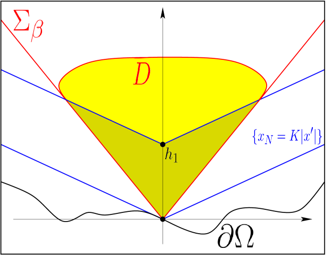
Figure 1. The set $D$ in the proof of Theorem 1.1-($iii$).

We introduce a continuous function $v$ satisfying

(4.12) $$\begin{cases}(-\Delta)^{s}v=0&\text{in $D$},\\ v=0&\text{in $(\mathbb{R}^{N}\setminus D)\cap\{x_{N}<K|x^{\prime}|+h_{1}\}$},\\ v=\varepsilon_{1}&\text{in $(\mathbb{R}^{N}\setminus D)\cap\{x_{N}>K|x^{\prime}|+h_{2}\}$},\\ 0\leqslant v\leqslant\varepsilon_{1}&\text{in $\mathbb{R}^{N}\setminus D$}.\end{cases}$$

By the maximum principle, $v>0$ in $D$, and hence by compactness there exists $\bar{C}>0$ such that

(4.13) $$\text{$v(x)\geqslant\bar{C}$ for any~{}$x$ such that~{}$B_{h_{1}\sin\beta}(x)\subseteq{D}$ and~{}$x_{N}\geqslant h_{1}$}.$$

Also, by (4.9), we have that $u\geqslant v$ in $\mathbb{R}^{N}\setminus D$. Furthermore, $(-\Delta)^{s}u\geqslant 0$ in $\Omega\supset D$, thanks to assumption ($f1$) and Theorem 1.1-($i$). Therefore, by the comparison principle in Theorem 1.8, we find that

(4.14) $$v\leqslant u \mathbb{R}^{N}$$ in .

Recalling (4.11), let now $r_{0}:=|x_{0}|\sin\beta=x_{0,N}\sin\beta$, and let us define

$$r_{k+1}:=r_{k}(1+\tan\beta)\quad\text{and}\quad x_{k+1}=x_{k}+\left(0^{\prime},\frac{r_{k}}{\cos\beta}\right)=\left(0^{\prime},x_{k,N}+\frac{r_{k}}{\cos\beta}\right),$$

see Figure 2.

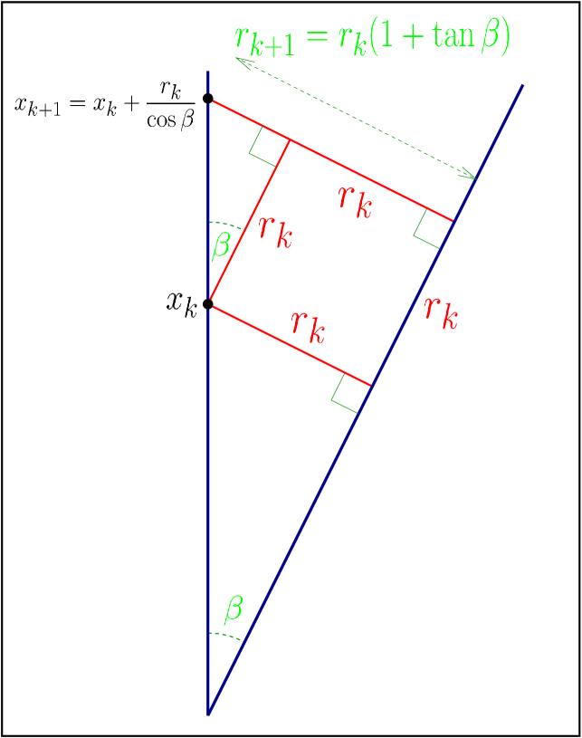
Figure 2. The geometry involved in the proof of Theorem 1.1-($iii$).

In this way $B_{r_{k}}(x_{k})\subset\Sigma_{\beta}$ for every $k$, and

(4.15) $$r_{k}=r_{0}(1+\tan\beta)^{k}=x_{0,N}\,\sin\beta(1+\tan\beta)^{k}.$$

As a consequence

(4.16) $$\begin{split}x_{k,N}&=x_{0,N}+\sum_{i=0}^{k-1}(x_{i+1,N}-x_{i,N})=x_{0,N}+\sum_{i=0}^{k-1}x_{0,N}\,\tan\beta\,(1+\tan\beta)^{i}\\ &=x_{0,N}+x_{0,N}\,\tan\beta\,\frac{(1+\tan\beta)^{k}-1}{\tan\beta}=x_{0,N}\,(1+\tan\beta)^{k},\end{split}$$

for every $k\in\mathbb{N}$.

We claim that

(4.17) $$\begin{split}&{\mbox{there exists a first natural number $k_{0}$ depending on $x_{0}$ such that }}\\ &x_{k_{0}}\in\{K|x^{\prime}|+h_{1}<x_{N}\}\quad\text{and}\quad B_{r_{k_{0}}}(x_{k_{0}})\subset\Sigma_{\beta}\cap B_{h_{2}}\subset D.\end{split}$$

Thanks to (4.15) and (4.16), and observing that by construction $x_{k}^{\prime}=0^{\prime}$ for every $k$, we see that $k_{0}\in\mathbb{N}$ has to be the minimum natural number satisfying

(4.18) $$x_{0,N}(1+\tan\beta)^{k_{0}}>h_{1}\quad\text{and}\quad x_{0,N}(1+\sin\beta)(1+\tan\beta)^{k_{0}}<h_{2},$$

that is

(4.19) $$\frac{\log\left(\frac{h_{1}}{x_{0,N}}\right)}{\log\left(1+\tan\beta\right)}\leqslant k_{0}\leqslant\frac{\log\left(\frac{h_{2}}{(1+\sin\beta)x_{0,N}}\right)}{\log\left(1+\tan\beta\right)}.$$

Notice that such a $k_{0}\in\mathbb{N}$ does exist, thanks to (4.10). This proves (4.17).

Furthermore, we remark that

$$\frac{\log\left(\frac{h_{1}}{x_{0,N}}\right)}{\log\left(1+\tan\beta\right)}=\mu_{1}-\nu_{1}\log(x_{0,N})\quad\text{and}\quad\frac{\log\left(\frac{h_{2}}{(1+\sin\beta)x_{0,N}}\right)}{\log\left(1+\tan\beta\right)}=\mu_{2}-\nu_{2}\log(x_{0,N})$$

for suitable $\mu_{1},\mu_{2}\in\mathbb{R}$, and $\nu_{1},\nu_{2}>0$, all depending only on $h_{1}$, $h_{2}$ and $\beta$. This and (4.19) say that

(4.20) $$\mu_{1}-\nu_{1}\,\log x_{0,N}\leqslant k_{0}\leqslant\mu_{2}-\nu_{2}\,\log x_{0,N}.$$

The previous construction implies that we have finite sequences of points $x_{k}$ and radii $r_{k}$, with $k=0,\dots,k_{0}$, such that

(4.21) $$B_{r_{k}}(x_{k})\subset D$$

for every $k=0,\dots,k_{0}$, and

$$|x_{k+1}-x_{k}|=x_{k+1,N}-x_{k,N}=\frac{r_{k}}{\cos\beta}=\frac{r_{k+1}}{\cos\beta(1+\tan\beta)}=:\rho_{\beta}r_{k+1},$$

with $\rho_{\beta}<1$ independent of $k$.

From (4.12) and (4.21), we deduce that $v$ is non-negative in $\mathbb{R}^{N}$ and $s$-harmonic in $B_{r_{k+1}}(x_{k+1})$, for any $k=0,\dots,k_{0}-1$. Hence, we are in position to apply the Harnack inequality in [12, Theorem 5.1], deducing that

$$v(x_{k+1})\leqslant\sup_{B_{\rho_{\beta}r_{k+1}}(x_{k+1})}v\leqslant\tilde{C}\inf_{B_{\rho_{\beta}r_{k+1}}(x_{k+1})}v\leqslant\tilde{C}v(x_{k})$$

for every $k=0,\dots,k_{0}-1$, where $\tilde{C}>0$ is a positive constant depending only on $\beta$.

Now we observe that

$$r_{k_{0}}=x_{0,N}\,\sin\beta(1+\tan\beta)^{k_{0}}\geqslant h_{1}\sin\beta,$$

thanks to (4.15) and (4.18). Similarly,

$$x_{k_{0},N}=x_{0,N}\,(1+\tan\beta)^{k_{0}}\geqslant h_{1},$$

thanks to (4.16) and (4.18).

As a consequence of this and of (4.13), we obtain that $v(x_{k_{0}})\geqslant\bar{C}$. Therefore, using (4.14) and (4.20), we obtain

$$u(x_{0}) \geqslant v(x_{0})\geqslant\frac{1}{\tilde{C}^{k_{0}}}v(x_{k_{0}})\geqslant\frac{\bar{C}}{e^{k_{0}\log\tilde{C}}}$$

$$\geqslant\frac{\bar{C}}{e^{\mu_{2}\log\tilde{C}}\cdot e^{-\nu_{2}\log\tilde{C}\log x_{0,N}}}=Cx_{0,N}^{\bar{\rho}}=C(x_{0,N}-\varphi(x_{0}^{\prime}))^{\bar{\rho}},$$

for some positive constants $C,\bar{\rho}$ depending only on $\beta$, $K$, $h_{1}$ and $h_{2}$.

This gives the desired point-wise estimate at the point $x_{0}$, with $x_{0}^{\prime}=0$ and $x_{0,N}\in(0,h_{1})$ (recall (4.11)), and with constants $C$ and $\bar{\rho}$ depending only on $\beta$, $K$, $h_{1}$ and $h_{2}$. Up to a translation, the same estimate holds at any point of $\Omega$, with vertical coordinate $x_{N}\in\big{(}\varphi(x^{\prime}),\,\varphi(x^{\prime})+h_{1}\big{)}$. That is, translating $\Sigma_{\beta}$ (and hence $D$) along the boundary $\partial\Omega$, the family $\{v(x-x_{0}):x_{0}\in\partial\Omega\}$ gives a wall of lower barriers for $u$, providing the desired lower estimate at any point of $\{\varphi(x^{\prime})<x_{N}<\varphi(x^{\prime})+h_{1}\}$, which completes the proof of Theorem 1.1-($iii$).∎

4.3. Uniqueness and monotonicity of the positive solution

This section is devoted to the proof of point ($v$) in Theorem 1.1. Our approach is inspired by [5, Section 5], but we modify it in such a way that the proof gives essentially in one shot both uniqueness and monotonicity of the solution. This simplifies the argument in [5], and completes the proof of Theorem 1.1.

We start with the preliminary observation that, under our assumptions, solutions are bounded away from $1$ if the distance from the boundary is finite (recall (4.1)).

Lemma 4.5.

For $h>0$, let

$$\Omega_{h}:=\{\varphi(x^{\prime})<x_{N}<\varphi(x^{\prime})+h\}.$$

Then, any bounded solution to (1.1) is bounded away from $1$ in $\Omega_{h}$, namely

$$\sup_{\overline{\Omega_{h}}}u<1.$$

Proof.

Let $u$ be a solution of (1.1), and let us suppose by contradiction that $u(x_{n})\to 1$ as $n\to+\infty$ along a sequence $\{x_{n}\}\subset\Omega_{h}$.

Let us consider then the sequence of translated functions $u_{n}(x):=u(x+x_{n})$. We observe that

(4.22) $$\lim_{n\to+\infty}u_{n}(0)=1$$

and

(4.23) $$\begin{cases}(-\Delta)^{s}u_{n}=f(u_{n})&\text{in $\Omega_{n}$},\\ u_{n}=0&\text{in $\mathbb{R}^{N}\setminus\Omega_{n}$},\\ 0\leqslant u_{n}\leqslant 1&\text{in $\mathbb{R}^{N}$},\end{cases}$$

where

$$\Omega_{n}:=\{x_{N}>\varphi(x^{\prime}+x^{\prime}_{n})-x_{n,N}\}.$$

Since $\varphi$ is globally Lipschitz continuous, the translated epigraphs $\Omega_{n}$ converge, up to subsequence, to a limit epigraph $\bar{\Omega}$, which is still globally Lipschitz continuous. Notice also that $\Omega_{n}$ satisfies a uniform cone condition, with opening of the cone independent of $n$. Thus, by Theorem 1.5, the sequence $\{u_{n}\}$ is uniformly bounded in $\mathcal{C}^{0,\alpha}(\mathbb{R}^{N})$, and hence converges locally uniformly in $\mathbb{R}^{N}$ to a limit function $\bar{u}\in\mathcal{C}^{0,\alpha}(\mathbb{R}^{N})$.

Thus, by (4.23) and the stability property of viscosity solutions [13, Lemma 4.5], we infer that $\bar{u}$ is a viscosity solution to

(4.24) $$\begin{cases}(-\Delta)^{s}\bar{u}=f(\bar{u})&\text{in $\bar{\Omega}$},\\ \bar{u}=0&\text{in $\mathbb{R}^{N}\setminus\bar{\Omega}$},\\ 0\leqslant\bar{u}\leqslant 1&\text{in $\mathbb{R}^{N}$}.\end{cases}$$

Actually, arguing as in [35, Remark 2.3], we see that $\bar{u}$ is a classical solution. Since also the function constantly equal to $1$ is a solution of the equation in (4.24) (recall that $f(1)=0$), the strong maximum principle implies that $\bar{u}<1$ in $\mathbb{R}^{N}$.

This is in contradiction with the fact that $\bar{u}(0)=1$, which follows from (4.22). ∎

In order to prove Theorem 1.1-($v$), let us consider two bounded solutions $u$ and $v$ of (1.1). We show that necessarily $u\geqslant v$. Exchanging the role of $u$ and $v$ we deduce also that $v\geqslant u$, whence uniqueness follows.

For this, first of all we observe that, by Theorem 1.1-($ii$), there exists $A>0$ such that

(4.25) $$u(x),v(x)>{t_{1}} {\rm dist}(x,\partial\Omega)>A$$ if ,

where ${t_{1}}$ was introduced in assumption ($f3$). Let

$$\Omega_{A}:=\left\{x\in\Omega:{\rm dist}(x,\partial\Omega)<A\right\}\quad{\mbox{ and }}\quad\Omega^{A}:=\Omega\setminus\overline{\Omega_{A}}.$$

Also, for $\tau\geqslant 0$ let us consider

$$u_{\tau}(x):=u(x+\tau e_{N}).$$

As in [5, Lemma 5.1], we show that:

Lemma 4.6.

If $u_{\tau}>v$ in $\Omega_{A}$, then $u_{\tau}>v$ in $\mathbb{R}^{N}$.

Proof.

First of all, since $\Omega$ is an epigraph we have

(4.26) if $$x\in\Omega^{A} x+\tau e_{N}\in\Omega^{A}$$, then .

Now we notice that $u_{\tau}\geqslant 0=v$ in $\mathbb{R}^{N}\setminus\Omega$. Thus, to establish the desired result, we have only to prove that

(4.27) $$u_{\tau}\geqslant v \Omega^{A}$$ in .

To this aim, we use (4.26) and we observe that

$$\begin{cases}(-\Delta)^{s}(v-u_{\tau})-c_{\tau}(x)(v-u_{\tau})=0\quad\text{in $\Omega^{A}$},\\ v-u_{\tau}\leqslant 0\quad\text{in $\mathbb{R}^{N}\setminus\Omega^{A}$},\end{cases}$$

where

$$c_{\tau}(x):=\begin{cases}\displaystyle\frac{f(v(x))-f(u_{\tau}(x))}{v(x)-u_{\tau}(x)}&\text{if $v(x)\neq u_{\tau}(x)$},\\ 0&\text{if $v(x)=u_{\tau}(x)$}.\end{cases}$$

Now we claim that

(4.28) $$u_{\tau},v\geqslant t_{1} \Omega^{A}$$ in .

Indeed, let $x\in\Omega^{A}$. Then $x+\tau e_{N}\in\Omega^{A}$, thanks to (4.26). Hence (4.28) follows from (4.25).

Now, since $f$ is non-increasing in $(t_{1},1)$, we deduce from (4.28) that $c_{\tau}\leqslant 0$ in $\Omega^{A}$, and by Lipschitz continuity we have also $c_{\tau}\in L^{\infty}(\Omega^{A})$.

Moreover, it is clear that $\Omega^{A}$ satisfies an exterior cone condition (since $\Omega$ does), and hence Theorem 1.8 and the strong maximum principle imply (4.27), as desired.∎

Now, we aim at showing that $u_{\tau}\geqslant v$ in $\mathbb{R}^{N}$ for $\tau=0$. Thanks to Lemma 4.6, this statement is equivalent to showing that $u_{\tau}\geqslant v$ in $\Omega_{A}$ for $\tau=0$.

By Lemma 4.5, we know that $v\leqslant C$ with $C<1$ in $\Omega_{A}$. Moreover, since $u\to 1$ uniformly as ${\rm dist}(x,\partial\Omega)\to+\infty$ (recall Theorem 1.1-($ii$)), we have that $u_{\tau}\geqslant v$ in $\Omega_{A}$ for $\tau$ sufficiently large. Therefore, we can define

(4.29) $$T:=\inf\left\{\tau>0:u_{t}>v\text{ in $\Omega_{A}$ for every $t>\tau$ }\right\}\in[0,+\infty).$$

Remark 4.7.

For the uniqueness, one could replace the previous definition of $T$ with

$$\inf\{\tau>0:u_{\tau}\geqslant v\text{ in $\Omega_{A}$}\},$$

as done in [5]. Nevertheless, as we will show later, definition (4.29) permits to perform the same argument used for the uniqueness also for the monotonicity of $u$.

We are now in the position of completing the proof of Theorem 1.1-($v$).

Completion of the proof of Theorem 1.1-($v$).

By continuity $u_{T}\geqslant v$ in $\Omega_{A}$. Hence, by Lemma 4.6,

(4.30) $$u_{T}\geqslant v \mathbb{R}^{N}$$ in .

Thus, if $T=0$ the proof is complete. To rule out the possibility that $T>0$, we argue by contradiction.

If $T>0$, then there exist sequences $0<\tau_{j}<T$ and $x_{j}\in\Omega_{A}$ such that

(4.31) $$\lim_{j\to+\infty}\tau_{j}=T>0$$

and

(4.32) $$u(x_{j}+\tau_{j}e_{N})\leqslant v(x_{j}).$$

Let us consider

$$u_{j}(x):=u(x+x_{j})\quad\text{and}\quad v_{j}(x):=v(x+x_{j}).$$

As in Lemma 4.5, we have that, up to subsequences, $u_{j}\to\bar{u}$ and $v_{j}\to\bar{v}$ locally uniformly, and $\bar{u}$ and $\bar{v}$ are solutions to (1.1) in a limit epigraph $\bar{\Omega}$.

We remark that, since $x_{j}\in\Omega$, the point $0$ belongs to the approximating domains and therefore

(4.33) $0$ belongs to the closure of $\bar{\Omega}$.

We also notice that

(4.34) $$\bar{u}_{T}(x):=\bar{u}(x+Te_{N})\geqslant\bar{v}(x) x\in\mathbb{R}^{N}$$ for any ,

thanks to (4.30). Furthermore, in light of (4.31), (4.32) and using the uniform convergence,

(4.35) $$\begin{split}&\bar{u}_{T}(0)=\bar{u}(Te_{N})=\lim_{j\to+\infty}u_{j}(\tau_{j}e_{N})=\lim_{j\to+\infty}u(x_{j}+\tau_{j}e_{N})\\ &\qquad\leqslant\lim_{j\to+\infty}v(x_{j})=\lim_{j\to+\infty}v_{j}(0)=\bar{v}(0).\end{split}$$

By (4.34) and (4.35), we conclude that

(4.36) $$\bar{u}_{T}(0)=\bar{v}(0).$$

Now we claim that

(4.37) $$\bar{u}_{T}>0=\bar{v} \partial\bar{\Omega}$$ on .

To check this, we take $\bar{p}\in\partial\bar{\Omega}$. Then there exists $x_{0}\in\partial\Omega$ such that $p_{j}:=x_{0}-x_{j}\to\bar{p}$ as $j\to+\infty$. As a consequence, using the uniform convergence, we see that

(4.38) $$\bar{v}(p)=\lim_{j\to+\infty}v_{j}(p)=\lim_{j\to+\infty}v_{j}(p_{j})=\lim_{j\to+\infty}v(p_{j}+x_{j})=v(x_{0})=0$$

and

(4.39) $$\begin{split}&\bar{u}_{T}(p)=\bar{u}(p+Te_{N})=\lim_{j\to+\infty}u_{j}(p+Te_{N})=\lim_{j\to+\infty}u_{j}(p_{j}+Te_{N})\\ &\qquad=\lim_{j\to+\infty}u(p_{j}+x_{j}+Te_{N})=u(x_{0}+Te_{N})>0,\end{split}$$

since $x_{0}+Te_{N}\in\Omega$ (here we are using that $T>0$). Combining (4.38) and (4.39), we obtain (4.37).

Also,

$$(-\Delta)^{s}(\bar{u}_{T}-\bar{v})-c_{T}(x)(\bar{u}_{T}-\bar{v})=0\qquad\text{in $\bar{\Omega}$},$$

where

$$c_{T}(x):=\begin{cases}\displaystyle\frac{f(\bar{u}_{T}(x))-f(\bar{v}(x))}{\bar{u}_{T}(x)-\bar{v}(x)},&\text{if $\bar{u}_{T}(x)\neq\bar{v}(x)$}\\ 0&\text{if $\bar{u}_{T}(x)=\bar{v}(x)$},\end{cases}$$

and $c_{T}\in L^{\infty}(\bar{\Omega})$. Thus, the strong maximum principle and (4.34) imply that either $\bar{u}_{T}>\bar{v}$ in $\bar{\Omega}$, or $\bar{u}_{T}\equiv\bar{v}$ in $\mathbb{R}^{N}$.

But the latter alternative is not admissible, due to (4.37). Therefore, we conclude that $\bar{u}_{T}>\bar{v}$ in $\bar{\Omega}$ and so, again by (4.37), in the closure of $\bar{\Omega}$. This is in contradiction with (4.33) and (4.36), hence the proof of Theorem 1.1-($v$) is complete. ∎

Proof of Theorem 1.1-($vi$).

We proceed exactly as for the uniqueness, but instead of comparing $u_{\tau}$ with $v$ we compare $u_{\tau}$ with $u$ (indeed, $v$ was just the generic solution, so the case $v:=u$ is admissible). In the end, we obtain that $u_{\tau}>u$ in $\Omega_{A}$ for every $\tau>0$, which by Lemma 4.6 yields the desired monotonicity. ∎

5. Monotonicity of solutions in coercive epigraphs

This section is devoted to the proof of Theorem 1.3, which rests upon the moving planes method. We introduce some notation: for $\lambda\in\mathbb{R}$, we set

$$\begin{split}T_{\lambda}&:=\{x\in\mathbb{R}^{N}:x_{N}=\lambda\};\\ H_{\lambda}&:=\{x\in\mathbb{R}^{N}:x_{N}<\lambda\};\\ x^{\lambda}&:=(x^{\prime},2\lambda-x_{N})\quad\text{the reflection of $x$ with respect to $T_{\lambda}$};\\ A^{\lambda}&:=\text{the reflection of a given set $A$ with respect to $T_{\lambda}$};\\ \Sigma_{\lambda}&:=H_{\lambda}\cap\Omega;\\ \lambda_{0}&:=\inf\left\{x_{N}:\text{there exists $x^{\prime}\in\mathbb{R}^{N}$ with $(x^{\prime},x_{N})\in\Omega$}\right\}.\end{split}$$

The crucial remark is that, since we deal with a coercive epigraph, the set $\Sigma_{\lambda}$ is bounded for every $\lambda\in\mathbb{R}$, even if $\Omega$ is unbounded. Therefore, one can adapt the proof of [29, Theorem 1.1], which uses the moving planes method for fractional elliptic equations in bounded domains. For the reader’s convenience, we recall the following weak maximum principle in sets of small measure, which we conveniently re-phrase for our purpose.

Proposition 5.1 (Proposition 2.2, [29]).

Let $D$ be an open and bounded subset of $\mathbb{R}^{N}$. Let $c\in L^{\infty}(D)$ with $\|c\|_{L^{\infty}(D)}<M$, and let $z$ be a solution to

(5.1) $$\begin{cases}(-\Delta)^{s}z\geqslant c(x)z&\text{in $D$},\\ z\geqslant 0&\text{in $\mathbb{R}^{N}\setminus D$}.\end{cases}$$

Then, there exists $\delta>0$ depending only on $N$, $s$ and $M$ such that if $|D|<\delta$ then $z\geqslant 0$ in $D$.

Remark 5.2.

Consider a sequence of boundary value problems of type (5.1), with $c=c_{n}$ and $D=D_{n}$, $n\in\mathbb{N}$. If we have a uniform bound $\|c_{n}\|_{L^{\infty}(D_{n})}<M$, then Proposition 5.1 gives a threshold $\delta$ independent of $n$.

Proof of Theorem 1.3.

We set $u_{\lambda}(x):=u(x^{\prime},2\lambda-x_{N})$ and $w_{\lambda}(x):=u_{\lambda}(x)-u(x)$.

We aim at proving that $w_{\lambda}>0$ in $H_{\lambda}$ for every $\lambda>\lambda_{0}$, which gives the desired monotonicity.

For any $\lambda>\lambda_{0}$, we have that $2\lambda-x_{N}>x_{N}$ in $\Sigma_{\lambda}$. Accordingly, the monotonicity of $f$ in $x_{N}$ gives

(5.2) $$\begin{split}(-\Delta)^{s}w_{\lambda}(x)&=(-\Delta)^{s}(u_{\lambda}(x)-u(x))\\ &=f(x^{\prime},2\lambda-x_{N},u_{\lambda}(x))-f(x,u(x))\\ &\geqslant f(x,u_{\lambda}(x))-f(x,u(x))\\ &=c_{\lambda}(x)w_{\lambda}(x)\end{split}$$

in $\Sigma_{\lambda}$, with

$$c_{\lambda}(x):=\begin{cases}\displaystyle\frac{f(x,u_{\lambda}(x))-f(x,u(x))}{u_{\lambda}(x)-u(x)}&\text{if $u_{\lambda}(x)\neq u(x)$},\\ 0&\text{if $u_{\lambda}(x)=u(x)$}.\end{cases}$$

Notice that, thanks to the Lipschitz continuity of $f$ and the fact that $u\in L^{\infty}_{\mathrm{loc}}(\mathbb{R}^{N})$, for any $\bar{\lambda}>\lambda_{0}$, there exists $C>0$ such that $\|c_{\lambda}\|_{L^{\infty}(\Sigma_{\lambda})}\leqslant C$ for any $\lambda\in(\lambda_{0},\bar{\lambda}]$.

For convenience, we now divide the proof into separate steps:

Step 1) We show that $w_{\lambda}>0$ in $\Sigma_{\lambda}$ for any $\lambda>\lambda_{0}$, with $\lambda-\lambda_{0}$ small enough.

For this, let $\Sigma_{\lambda}^{-}:=\{x\in\Sigma_{\lambda}:w_{\lambda}(x)<0\}$. We first show that

(5.3) $$w_{\lambda}\geqslant 0 \Sigma_{\lambda} \lambda>\lambda_{0} \lambda-\lambda_{0}$$ in for any , with  small enough,

i.e., that $\Sigma_{\lambda}^{-}=\varnothing$. To this aim, we argue by contradiction. If $\Sigma_{\lambda}^{-}\neq\varnothing$, we can define

(5.4) $$w_{1,\lambda}:=\begin{cases}w_{\lambda}&\text{in $\Sigma_{\lambda}^{-}$}\\ 0,&\text{in $\mathbb{R}^{N}\setminus\Sigma_{\lambda}^{-}$},\end{cases}\qquad{\mbox{ and }}\qquad w_{2,\lambda}:=\begin{cases}w_{\lambda}&\text{in $\mathbb{R}^{N}\setminus\Sigma_{\lambda}^{-}$},\\ 0&\text{in $\Sigma_{\lambda}^{-}$}.\end{cases}$$

We observe that $w_{\lambda}=w_{1,\lambda}+w_{2,\lambda}$, and that $w_{1,\lambda}\leqslant 0$ while $w_{2,\lambda}\geqslant 0$. Exactly as in [29, Theorem 1.1, step 1], it is possible to show that $(-\Delta)^{s}w_{2,\lambda}\leqslant 0$ in $\Sigma_{\lambda}^{-}$. Hence, by (5.2),

$$\begin{cases}(-\Delta)^{s}w_{1,\lambda}\geqslant c_{\lambda}(x)w_{1,\lambda}&\text{in $\Sigma_{\lambda}^{-}$},\\ w_{1,\lambda}=0&\text{in $\mathbb{R}^{N}\setminus\Sigma_{\lambda}^{-}$}.\end{cases}$$

Thus, by the maximum principle in sets of small measure (see Proposition 5.1), we infer that, for any $\lambda>\lambda_{0}$ close to $\lambda_{0}$, it results that $w_{\lambda}\geqslant 0$ in $\mathbb{R}^{N}$. As a consequence, $w_{1,\lambda}=w_{\lambda}\geqslant 0$ in $\Sigma^{-}_{\lambda}$, which proves (5.3).

As a side remark, we notice that here we do not need $u\in L^{\infty}(\mathbb{R}^{N})$, but only $u\in L^{\infty}_{\mathrm{loc}}(\mathbb{R}^{N})$ (which follows automatically by the definition of classical or even viscosity solution), since $\Sigma_{\lambda}$ is bounded.

Now we claim that

(5.5) $$\text{if $\lambda>\lambda_{0}$ and $w_{\lambda}\geqslant 0$ in $\Sigma_{\lambda}$, then $w_{\lambda}>0$ in $\Sigma_{\lambda}$}.$$

This is not a consequence of the strong maximum principle since the function $w_{\lambda}$ changes sign, by definition.

By contradiction, let us suppose that there exists $x_{0}\in\Sigma_{\lambda}$ such that $u_{\lambda}(x_{0})=u(x_{0})$. Since $|x_{0}-y|<|x_{0}-y_{\lambda}|$ for every $x_{0}\in\Sigma_{\lambda}$ and $y\in H_{\lambda}$, and $w_{\lambda}$ is positive in a subset of $H_{\lambda}$ having positive measure, we deduce that

$$0 =c_{\lambda}(x_{0})\,w_{\lambda}(x_{0})\leqslant(-\Delta)^{s}w_{\lambda}(x_{0})=-\int_{H_{\lambda}}\frac{w_{\lambda}(y)}{|x-y|^{N+2s}}\,dy-\int_{\mathbb{R}^{N}\setminus H_{\lambda}}\frac{w_{\lambda}(y)}{|x-y|^{N+2s}}\,dy$$

$$=-\int_{H_{\lambda}}w_{\lambda}(y)\left(\frac{1}{|x-y|^{N+2s}}-\frac{1}{|x-y_{\lambda}|^{N+2s}}\right)\,dy<0,$$

where (5.2) was used, and so we obtain a contradiction.

This proves (5.5). Then, the desired result in Step 1 follows by combining (5.3) and (5.5).

Step 2) We show that $w_{\lambda}>0$ in $\Sigma_{\lambda}$ for every $\lambda>\lambda_{0}$. Let

$$\tilde{\lambda}:=\sup\{\lambda>\lambda_{0}:\text{$w_{\mu}>0$ in $\Sigma_{\mu}$ for every $\mu\in(\lambda_{0},\tilde{\lambda})$}\}.$$

By the previous step $\tilde{\lambda}>\lambda_{0}$. If $\tilde{\lambda}=+\infty$ the proof of Step 2 is complete, and hence we argue by contradiction supposing that $\tilde{\lambda}<+\infty$.

By continuity and by (5.5) we have

(5.6) $$w_{\tilde{\lambda}}>0 \Sigma_{\tilde{\lambda}}$$ in .

Let us consider now

$$m:=\sup_{\lambda\in(\lambda_{0},\tilde{\lambda}+1]}\|c_{\lambda}\|_{L^{\infty}(\Sigma_{\lambda})}.$$

This value is finite since $u\in L^{\infty}_{\mathrm{loc}}(\mathbb{R}^{N})$, $f$ is locally Lipschitz, and $\Sigma_{\tilde{\lambda}+1}$ is bounded. Therefore, the threshold $\delta=\delta(N,s,m)$ for the maximum principle in domains of small measure in Proposition 5.1 is well defined (recall Remark 5.2).

Let us fix a compact set $K\Subset\Sigma_{\tilde{\lambda}}$ such that

(5.7) $$|\Sigma_{\tilde{\lambda}}\setminus K|<\frac{\delta}{2}.$$

By compactness and (5.6), we have that

$$\inf_{K}w_{\tilde{\lambda}}>0.$$

Using this and (5.7), we have that, by continuity, there exists $\bar{\varepsilon}>0$ small enough such that

(5.8) $$|\Sigma_{\tilde{\lambda}+\varepsilon}\setminus K|<\delta\qquad{\mbox{ and }}\qquad\inf_{K}w_{\tilde{\lambda}+\varepsilon}>0$$

for every $\varepsilon\in(0,\bar{\varepsilon})$.

Let now $\Sigma_{\tilde{\lambda}+\varepsilon}^{-}:=\Sigma_{\tilde{\lambda}+\varepsilon}\cap\{w_{\tilde{\lambda}+\varepsilon}<0\}$. We observe that

(5.9) the measure of $$\Sigma_{\tilde{\lambda}+\varepsilon}^{-} \delta$$ is smaller than ,

thanks to (5.8).

Now, we consider the functions $w_{1,\tilde{\lambda}+\varepsilon}$ and $w_{2,\tilde{\lambda}+\varepsilon}$ defined as in (5.4) with $\lambda:=\tilde{\lambda}+\varepsilon$. Proceeding as in Step 1, we can check that

$$(-\Delta)^{s}w_{1,\tilde{\lambda}+\varepsilon}\geqslant c_{\tilde{\lambda}+\varepsilon}(x)w_{1,\tilde{\lambda}+\varepsilon}\qquad\text{in $\Sigma_{\tilde{\lambda}+\varepsilon}^{-}$}.$$

We use this, (5.9) and the maximum principle in sets of small measure (see Proposition 5.1) to conclude that $w_{1,\tilde{\lambda}+\varepsilon}\geqslant 0$ in $\mathbb{R}^{N}$ for every $\varepsilon$ sufficiently small.

As a consequence, recalling (5.4), we have that $w_{\tilde{\lambda}+\varepsilon}\geqslant w_{1,\tilde{\lambda}+\varepsilon}\geqslant 0$. Therefore, from (5.5) we conclude that $w_{\tilde{\lambda}+\varepsilon}>0$ in $\Sigma_{\tilde{\lambda}+\varepsilon}$ for any $\varepsilon>0$ small enough, in contradiction with the definition of $\tilde{\lambda}$. ∎

6. Overdetermined problems

This section concerns the study of the overdetermined problem (1.4), where $\Omega$ is a globally Lipschitz epigraph, satisfying the additional flatness assumption (1.5). Regarding $f$, it satisfies ($f1$)-($f3$) in the introduction. As in the proof of Theorem 1.1, it is not not restrictive to suppose that $\mu=1$.

In particular, we now proceed with the proof of Theorem 1.4, which is the fractional counterpart of the proof of Theorem 7.1 in [5], where the local case was considered.

Proof of Theorem 1.4.

We claim that for any $\tau^{\prime}\in\mathbb{R}^{N-1}$

(6.1) $$\Omega\subseteq\Omega-(\tau^{\prime},0)=\{x:(x^{\prime}+\tau^{\prime},x_{N})\in\Omega\}.$$

To this extent, for $\tau=(\tau^{\prime},0)$ fixed and $h\geqslant 0$, let us consider

$$\Sigma_{h,\tau}:=\Omega-\tau-he_{N}=\{x\in\mathbb{R}^{N}\,:\;(x^{\prime}+\tau^{\prime},x_{N}+h)\in\Omega\}.$$

Since $\varphi$ is Lipschitz continuous, for $h>0$ sufficiently large we have that $\Sigma_{h,\tau}$ contains strictly $\Omega$. In other words, we can define the real number

(6.2) $$h^{*}:=\inf\left\{h\geqslant 0:\Sigma_{k,\tau}\supset\Omega\text{ for every $k>h$}\right\}.$$

We claim that

(6.3) $$h^{*}=0.$$

To prove this, let us suppose by contradiction that $h^{*}>0$. Then there exist sequences $0<h_{j}<h^{*}$ and $x_{j}\in\Omega\setminus\Sigma_{h_{j},\tau}$ with

$$\lim_{j\to+\infty}h_{j}=h^{*}>0.$$

By assumption (1.5), we infer that $\{x_{j}\}$ is bounded, and hence up to a subsequence $x_{j}\to a$, for some $a\in\overline{\Omega\setminus\Sigma_{h^{*},\tau}}\subseteq\overline{\Omega}\setminus\Sigma_{h^{*},\tau}$.

On the other hand, by (6.2), we know that $\Sigma_{h^{*},\tau}\supseteq\Omega$ and therefore $a\in\partial\Omega\cap\partial\Sigma_{h^{*},\tau}$. In other words, the set $\Omega$ is internally tangent to $\Sigma_{h^{*},\tau}$ in $a$.

Now, let us consider, for $h\geqslant h^{*}$,

$$u_{h,\tau}(x):=u(x+\tau+he_{N}).$$

We claim that

(6.4) $$u_{h^{*},\tau}\geqslant u\qquad\text{in $\mathbb{R}^{N}$}.$$

To this aim, we argue as in Subsection 4.3. First, we introduce $A>0$ large enough, so that both $u$ and $u_{h^{*},\tau}$ are larger than $t_{1}$ in $\Omega^{A}:=\{{\rm dist}(x,\partial\Omega)>A\}$ ($t_{1}$ is defined in assumption ($f3$)).

Then, for any $h\geqslant h^{*}$, we have that $u_{h,\tau}\geqslant t_{1}$ in $\Omega^{A}$, and $u_{h,\tau}\geqslant 0=u$ in $\mathbb{R}^{N}\setminus\Omega$.

By Lemma 4.5 and Theorem 1.1 applied to $u$, we know that $u_{h,\tau}\geqslant u$ in $\Omega_{A}=\Omega\setminus\overline{\Omega^{A}}$ if $h$ is sufficiently large. Therefore we can define

$$\tilde{h}:=\inf\{h>h^{*}:u_{k,\tau}\geqslant u\text{ in $\Omega_{A}$ for every $k>h$}\}.$$

If $\tilde{h}=h^{*}$, then claim (6.4) follows from Lemma 4.6. On the other hand, if $\tilde{h}>h^{*}$ it is not difficult to obtain a contradiction as in Subsection 4.3, thus completing the proof of (6.4).

Moreover, by internal tangency, the outer normal to $\partial\Omega$ and to $\partial\Sigma_{h^{*},\tau}$ coincide at the point $a$. Accordingly, by the $s$-Neumann condition in (1.4) reads

(6.5) $$(\partial_{\nu})_{s}u(a)-(\partial_{\nu})_{s}u_{h^{*},\tau}(a)=0.$$

On the other hand, the function $w_{h^{*},\tau}:=u_{h^{*},\tau}-u$ satisfies

$$\begin{cases}(-\Delta)^{s}w_{h^{*},\tau}-c_{h^{*},\tau}(x)w_{h^{*},\tau}=0&\text{in $\Omega$},\\ w_{h^{*},\tau}\geqslant 0&\text{in $\mathbb{R}^{N}$},\end{cases}$$

where

$$c_{h^{*},\tau}(x):=\begin{cases}\displaystyle\frac{f(u_{h^{*},\tau}(x))-f(u(x))}{u_{h^{*},\tau}(x)-u(x)}&\text{if $u_{h^{*},\tau}(x)\neq u(x)$},\\ 0&\text{if $u_{h^{*},\tau}(x)=u(x)$}.\end{cases}$$

Therefore, the Hopf lemma for the fractional Laplacian (see [30, Lemma 1.2]) gives

$$0>(\partial_{\nu})_{s}w_{h^{*},\tau}(a)=(\partial_{\nu})_{s}u_{h^{*},\tau}(a)-(\partial_{\nu})_{s}u(a),$$

in contradiction with (6.5). This proves (6.3).

Using (6.3), we deduce that

$$\Sigma_{0,\tau}=\Omega-\tau\supseteq\Omega,$$

which in turn implies (6.1).

Now, we deduce from (6.1) that the function $\varphi$ is necessarily a constant, i.e. $\Omega$ is a half-space (and this concludes the proof of Theorem 1.4).

Indeed, if by contradiction $\varphi$ is not constant there exist $x_{1}^{\prime},x_{2}^{\prime}\in\mathbb{R}^{N-1}$ such that $\varphi(x_{1}^{\prime})<\varphi(x_{2}^{\prime})$. Let $y:=(\varphi(x_{1}^{\prime})+\varphi(x_{2}^{\prime}))/2$. Notice that $\varphi(x_{1}^{\prime})<y<\varphi(x_{2}^{\prime})$, and therefore

(6.6) $$(x_{2}^{\prime},y)\not\in\Omega\quad{\mbox{ and }}\quad(x_{1}^{\prime},y)\in\Omega.$$

Thus, using (6.1) with $\tau^{\prime}:=x_{2}^{\prime}-x_{1}^{\prime}$, we obtain that

$$(x_{1}^{\prime},y)=x_{1}\in\Omega\subseteq\Omega-(x_{2}^{\prime}-x_{1}^{\prime},0).$$

By adding $(x_{2}^{\prime}-x_{1}^{\prime},0)$ to this inclusion, we find that $(x_{2}^{\prime},y)\in\Omega$, which is in contradiction with (6.6). ∎

References

- [1] R. Bañuelos and K. Bogdan. Symmetric stable processes in cones. Potential Anal., 21(3):263–288, 2004.
- [2] B. Barrios, L. Del Pezzo, J. García-Melián and A. Quaas. Monotonicity of solutions for some nonlocal elliptic problems in half-spaces. Preprint arXiv: 1606.01061, 2016.
- [3] B. Barrios, L. Montoro, and B. Sciunzi. On the moving plane method for nonlocal problems in bounded domains. Preprint arXiv: 1405.5402, 2014.
- [4] H. Berestycki, L. Caffarelli, and L. Nirenberg. Further qualitative properties for elliptic equations in unbounded domains. Ann. Scuola Norm. Sup. Pisa Cl. Sci. (4), 25(1-2):69–94 (1998), 1997. Dedicated to Ennio De Giorgi.
- [5] H. Berestycki, L. A. Caffarelli, and L. Nirenberg. Monotonicity for elliptic equations in unbounded Lipschitz domains. Comm. Pure Appl. Math., 50(11):1089–1111, 1997.
- [6] H. Berestycki and L. Nirenberg. On the method of moving planes and the sliding method. Bol. Soc. Brasil. Mat. (N.S.), 22(1):1–37, 1991.
- [7] K. Bogdan. The boundary Harnack principle for the fractional Laplacian. Studia Math., 123(1):43–80, 1997.
- [8] X. Cabré and E. Cinti. Energy estimates and 1-D symmetry for nonlinear equations involving the half-Laplacian. Discrete Contin. Dyn. Syst., 28(3):1179–1206, 2010.
- [9] X. Cabré and E. Cinti. Sharp energy estimates for nonlinear fractional diffusion equations. Calc. Var. Partial Differential Equations, 49(1-2):233–269, 2014.
- [10] X. Cabré and Y. Sire. Nonlinear equations for fractional Laplacians, I: Regularity, maximum principles, and Hamiltonian estimates. Ann. Inst. H. Poincaré Anal. Non Linéaire, 31(1):23–53, 2014.
- [11] X. Cabré and Y. Sire. Nonlinear equations for fractional Laplacians II: Existence, uniqueness, and qualitative properties of solutions. Trans. Amer. Math. Soc., 367(2):911–941, 2015.
- [12] L. Caffarelli and L. Silvestre. An extension problem related to the fractional Laplacian. Comm. Partial Differential Equations, 32(7-9):1245–1260, 2007.
- [13] L. Caffarelli and L. Silvestre. Regularity theory for fully nonlinear integro-differential equations. Comm. Pure Appl. Math., 62(5):597–638, 2009.
- [14] L. Caffarelli and L. Silvestre. The Evans-Krylov theorem for nonlocal fully nonlinear equations. Ann. of Math. (2), 174(2):1163–1187, 2011.
- [15] W. Chen, C. Li, Y. Li. A direct method of moving planes for the fractional Laplacian. Preprint arXiv:1411.1697, 2014.
- [16] C. Cortázar, M. Elgueta, and J. García-Melián. Nonnegative solutions of semilinear elliptic equations in half-spaces. J. Math. Pures Appl. (9), 106(5):866–876, 2016.
- [17] A.-L. Dalibard and D. Gérard-Varet. On shape optimization problems involving the fractional Laplacian. ESAIM Control Optim. Calc. Var., 19(4):976–1013, 2013.
- [18] E. N. Dancer. Some remarks on half space problems. Discrete Contin. Dyn. Syst., 25(1):83–88, 2009.
- [19] J. Dávila, L. Dupaigne, J. Wei. On the fractional Lane-Emden equation. Trans. Amer. Math. Soc., in press. Preprint arXiv: 1404.3694, 2014.
- [20] S. Dipierro, L. Montoro, I. Peral, and B. Sciunzi. Qualitative properties of positive solutions to nonlocal critical problems involving the Hardy-Leray potential. Calc. Var. Partial Differential Equations, 55(4), 55:99, 2016.
- [21] S. Dipierro, O. Savin, and E. Valdinoci. A nonlocal free boundary problem. SIAM J. Math. Anal., 47(6):4559–4605, 2015.
- [22] S. Dipierro, N. Soave, and E. Valdinoci. On fractional elliptic equations in Lipschitz sets and epigraphs: Regularity, monotonicity and rigidity results. Preprint http://www.wias-berlin.de/preprint/2256/wias_preprints_2256.pdf, 2016.
- [23] M. J. Esteban and P.-L. Lions. Existence and nonexistence results for semilinear elliptic problems in unbounded domains. Proc. Roy. Soc. Edinburgh Sect. A, 93(1-2):1–14, 1982/83.
- [24] M. M. Fall and S. Jarohs. Overdetermined problems with fractional Laplacian. ESAIM Control Optim. Calc. Var., 21(4):924–938, 2015.
- [25] M. M. Fall and T. Weth. Monotonicity and nonexistence results for some fractional elliptic problems in the half-space. Commun. Contemp. Math., 18(1):1550012, 25, 2016.
- [26] A. Farina and B. Sciunzi. Qualitative properties and classification of nonnegative solutions to in unbounded domains when . Preprint arXiv:1405.3428, 2014.
- [27] A. Farina and N. Soave. Symmetry and uniqueness of nonnegative solutions of some problems in the halfspace. J. Math. Anal. Appl., 403(1):215–233, 2013.
- [28] M. Fazly and J. Wei On stable solutions of the fractional Henon-Lane-Emden equation. Commun. Contemp. Math., 18(5):1650005, 24, 2016.
- [29] P. Felmer and Y. Wang. Radial symmetry of positive solutions to equations involving the fractional Laplacian. Commun. Contemp. Math., 16(1):1350023, 24, 2014.
- [30] A. Greco and R. Servadei. Hopf’s lemma and constrained radial symmetry for the fractional Laplacian. Preprint: https://www.ma.utexas.edu/mp_arc/c/14/14-69.pdf, 2014.
- [31] G. Grubb. Local and nonlocal boundary conditions for -transmission and fractional elliptic pseudodifferential operators. Anal. PDE, 7(7):1649–1682, 2014.
- [32] G. Grubb. Fractional Laplacians on domains, a development of Hörmander’s theory of -transmission pseudodifferential operators. Adv. Math., 268:478–528, 2015.
- [33] S. Jarohs. Symmetry of solutions to nonlocal nonlinear boundary value problems in radial sets. NoDEA Nonlinear Differential Equations Appl., 23(3):22, Art. 32, 2016.
- [34] D. Li , Z. Li. Some overdetermined problems for the fractional Laplacian equation on the exterior domain and the annular domain. Nonlinear Anal.: TMA, 139:196–210, 2016.
- [35] A. Quaas and A. Xia. Liouville type theorems for nonlinear elliptic equations and systems involving fractional Laplacian in the half space. Calc. Var. Partial Differential Equations, 52(3-4):641–659, 2015.
- [36] X. Ros-Oton and J. Serra. Boundary regularity estimates for nonlocal elliptic equations in and domains. Preprint arXiv:1512.07171, 2015.
- [37] X. Ros-Oton and J. Serra. Boundary regularity for fully nonlinear integro-differential equations. Duke Math. J., 165(11):2079-–2154, 2016.
- [38] X. Ros-Oton and J. Serra. The Dirichlet problem for the fractional Laplacian: regularity up to the boundary. J. Math. Pures Appl. (9), 101(3):275–302, 2014.
- [39] O. Savin and E. Valdinoci. -convergence for nonlocal phase transitions. Ann. Inst. H. Poincaré Anal. Non Linéaire, 29(4):479–500, 2012.
- [40] O. Savin and E. Valdinoci. Some monotonicity results for minimizers in the calculus of variations. J. Funct. Anal., 264(10):2469–2496, 2013.
- [41] L. Silvestre. Hölder estimates for solutions of integro-differential equations like the fractional Laplace. Indiana Univ. Math. J., 55(3):1155–1174, 2006.
- [42] L. Silvestre. Regularity of the obstacle problem for a fractional power of the Laplace operator. Comm. Pure Appl. Math., 60(1):67–112, 2007.
- [43] Y. Sire and E. Valdinoci. Fractional Laplacian phase transitions and boundary reactions: a geometric inequality and a symmetry result. J. Funct. Anal., 256(6):1842–1864, 2009.
- [44] N. Soave and E. Valdinoci. Overdetermined problems for the fractional Laplacian in exterior or annular sets. J. Anal. Math., in press. Preprint arXiv: 1412.5074, 2014.