Using Indirect Encoding of Multiple Brains to Produce Multimodal Behavior

Abstract

An important challenge in neuroevolution is to evolve complex neural networks with multiple modes of behavior. Indirect encodings can potentially answer this challenge. Yet in practice, indirect encodings do not yield effective multimodal controllers. Thus, this paper introduces novel multimodal extensions to HyperNEAT, a popular indirect encoding. A previous multimodal HyperNEAT approach called situational policy geometry assumes that multiple brains benefit from being embedded within an explicit geometric space. However, experiments here illustrate that this assumption unnecessarily constrains evolution, resulting in lower performance. Specifically, this paper introduces HyperNEAT extensions for evolving many brains without assuming geometric relationships between them. The resulting Multi-Brain HyperNEAT can exploit human-specified task divisions to decide when each brain controls the agent, or can automatically discover when brains should be used, by means of preference neurons. A further extension called module mutation allows evolution to discover the number of brains, enabling multimodal behavior with even less expert knowledge. Experiments in several multimodal domains highlight that multi-brain approaches are more effective than HyperNEAT without multimodal extensions, and show that brains without a geometric relation to each other outperform situational policy geometry. The conclusion is that Multi-Brain HyperNEAT provides several promising techniques for evolving complex multimodal behavior.

I Introduction

Success in many AI domains requires agents capable of complex multimodal behavior, i.e. agents able to switch between distinct policies based on environmental context. Humans excel in this regard, as they can switch fluidly between both physical (sports, dancing, labor) and intellectual (planning, writing, problem solving) tasks. Such behavior is vital for a general AI agent, and necessary for more focused agents as well, such as robots, video game agents, and agents in artificial life simulations.

One promising approach for creating policies for agents is neuroevolution [1, 2], i.e. evolving artificial neural networks (ANNs). While there exist multimodal methods for neuroevolution [3, 4], many are direct encodings, i.e. each component of an ANN is explicitly and distinctly encoded. However, such direct encodings cannot exploit regularities among inputs and outputs, and do not scale well to problems requiring large ANNs, motivating indirect encodings that can compactly represent large networks. For these reasons, indirect encodings capable of multimodal behavior are an important area of research.

This paper thus proposes new extensions to a popular indirect encoding called HyperNEAT [5]. A previous multimodal extension to HyperNEAT is situational policy geometry [6], an approach that creates separate controllers for different situations defined by a human-specified task division. However, there are three problems with this approach. First, situational policy geometry requires there to be a geometric relationship between different controllers (e.g. advancing and retreating are geometric opposites). But in practice, an agent may need distinct policies that are not geometrically related. Second, the human-specified task division that is required imposes a burden of expert knowledge. However, it is not always clear when different modes of behavior should be used. Third, the number of policies to generate must be set in advance, requiring additional human knowledge.

A direct-encoded approach to learning multimodal behavior without these limitations is Modular Multiobjective NEAT (MM-NEAT [7, 4]). MM-NEAT networks have several output modules, each of which defines a different policy. These policies are not geometrically related, and evolution can decide when each policy should be activated using preference neurons. When combined with module mutation [8, 4], evolution can add modules as needed without human intervention.

However, because MM-NEAT is a direct encoding, it cannot exploit regularities among inputs and outputs. Further, because in direct encodings a network’s parameter count is proportional to its size (i.e. the curse of dimensionality), such methods struggle to evolve complex ANNs; note that this second advantage is not directly tested in this paper but is a well-known property of HyperNEAT [9, 10, 11]. The motivation for this paper’s approach is thus to combine HyperNEAT with MM-NEAT to leverage the advantages of both: indirectly encoded controllers can better scale and exploit domain regularities, while MM-NEAT allows evolution to create new modules and discover how to arbitrate between them (without assuming any geometric relationship between modules). The result is a system called Multi-Brain HyperNEAT (MB-HyperNEAT).

MB-HyperNEAT is evaluated in four representative multimodal domains, including two introduced in this paper. The results indicate that policies unconstrained by geometry outperform situational policy geometry. Additionally, when preference neurons are used to allow evolution to discover how and when to use each brain, agents outperform standard HyperNEAT (without multimodal extensions). In this way, MB-HyperNEAT highlights the possible benefits from porting previous multimodal approaches to indirect encodings in a principled way.

II Background

This section discusses previous approaches to evolving multimodal behavior, and then describes HyperNEAT, which the approaches in this paper extend in a manner similar to yet distinct from situational policy geometry, which is also explained.

II-A Evolving Multimodal Behavior

Because complex domains often encompass many diverse and distinct subtasks, agents in such domains must exhibit multimodal behavior to succeed. For example, being able to defend and advance the ball in soccer, or exhibiting offensive and defensive behavior in a video game. The Universal Approximation Theorem [12] indicates that a properly configured neural network can theoretically exhibit any behavior, which includes multimodal behavior. However, in practice such behavior is more effectively produced by modular networks, as the examples below demonstrate.

Modular ANNs correspond to structures seen in biology, and can represent distinct policies for the subtasks within a multimodal domain. For these reasons, modular ANNs are an active area of research [13, 14, 15]. Most multimodal approaches either implement evolutionary mechanisms that encourage modularity [13, 14] or explicitly divide ANNs into modules that can specialize to different tasks [16, 3, 4, 17].

Another approach that easily allows for multiple modes of behavior is to use several distinct networks to make decisions. An example of this approach is Neural Learning Classifier Systems [18, 19, 20], in which a single agent is controlled by a population of neural networks, subsets of which activate to handle particular situations. During learning, activated networks are generally modified according to a rule similar to that used in temporal difference learning. Individual networks also accrue fitness whenever activated, and a genetic algorithm is periodically or probabilistically used to allow offspring of fitter networks to replace less fit networks.

Multiple distinct networks can also be combined to control a single agent if a human trains or evolves each component separately, and then combines them in a hierarchical configuration. For example, Togelius’s evolved subsumption architecture [21] was used in EvoTanks [22] and Unreal Tournament [23]. Lessin et al. used the principles of encapsulation, syllabus, and pandemonium to evolve complex behavior for virtual creatures [24, 25]. These approaches still require a programmer to divide the domain into constituent tasks and develop effective training scenarios for each task.

The primary inspiration for this paper is individual networks divided into explicit modules. This approach allows an agent to have distinct output modules corresponding to separate policies meant to be used in different situations. Networks can either have a human-designated module for each task, as with Multitask Learning [26], or evolution can discover when and how to use each module through special preference neurons. When an ANN with preference neurons is evaluated, the module whose preference neuron has the highest activation determines the final output. Preference neurons can also be combined with module mutation [8], an operation that adds new modules, freeing the experimenter from fixing the number in advance.

This paper adapts these ideas to extend HyperNEAT, which is described next.

II-B HyperNEAT

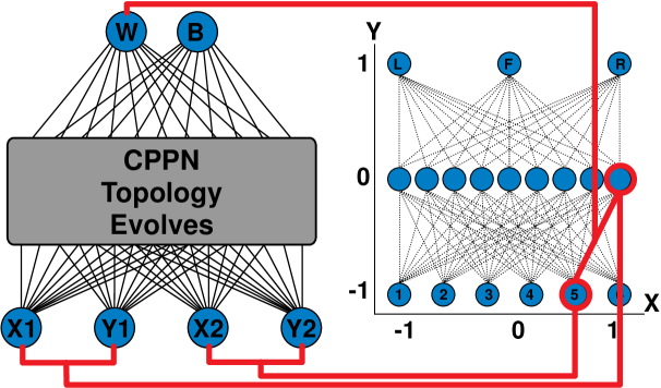
(a) Standard HyperNEAT (One Brain)

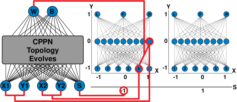
(b) Situational Policy Geometry

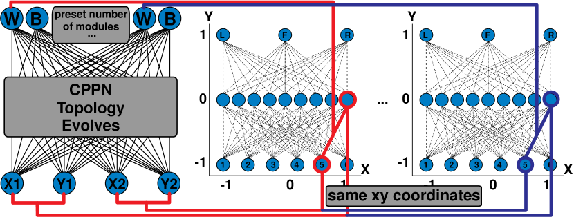
(c) Multitask

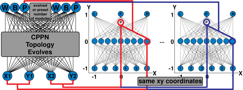
(d) Preference Neurons

Figure 1: Methods for Generating Substrate Brains. Each figure shows a CPPN on the left and the corresponding substrate brain(s) it produces on the right. Each successive figure adds new features: situational policy geometry encodes multiple brains, multitask encodes brains without geometric relationships, and preference neurons specify when to switch brains. LABEL:sub@fig:1M Standard HyperNEAT [5]: The CPPN creates a single-brain substrate. Dotted lines in the substrate indicate which neurons can be connected. For each possible connection, the xy-coordinates of both neurons are input into the CPPN. The CPPN output $W$ determines whether a connection is created, and if it is, what its weight value will be. The $B$ output determines a fixed bias from $(0,0)$ to each substrate neuron (not shown). LABEL:sub@fig:SPG Situational policy geometry [6]: CPPNs have an additional input $S$, which defines a space of possible brains. The substrate contains a separate brain for each value of $S$ the CPPN is queried with. Brains for $S$ values of $-1$ and $1$ are shown. The next two approaches are new to this work: LABEL:sub@fig:MT Multitask: The CPPN has no additional inputs, but instead has a separate group of outputs for each distinct brain. Each brain is encoded independently, rather than being embedded along an explicit $S$ dimension. When the CPPN is queried with a pair of neuron coordinates, each output module supplies the corresponding connection weight for a different brain. LABEL:sub@fig:Pref Preference neurons: When using preference neurons, the number of modules can either be preset or evolved using module mutation (Figure 2). Preference neuron brains are generated similarly to multitask brains, except that each output module of the CPPN has an additional neuron $P$ that is queried only when the postsynaptic neuron whose xy-coordinates are being input is a preference neuron. The preference neuron (white) of each brain is embedded in the substrate at coordinate $(0,0.8)$, and is queried for potential connections to all neurons in the hidden and input layers. All brains are activated on each time step, but only the one with the highest preference neuron output determines the agent’s behavior on a given time step.

Hypercube-based Neuro-Evolution of Augmenting Topologies (HyperNEAT [5]) is an extension of NEAT [1], a direct encoding that evolves arbitrary-topology ANNs through mutations that gradually complexify networks. HyperNEAT uses NEAT as a mechanism to specify connectivity patterns across an indirectly-encoded substrate ANN.

Such connectivity patterns are represented by Compositional Pattern Producing Networks (CPPNs), which differ from NEAT networks in that (1) different neurons can have different activation functions chosen from a hand-designed set, and (2) they are intended to be queried repeatedly across a coordinate space to produce a pattern. The activation function set includes functions that can produce useful ANN connectivity patterns, e.g. symmetry and repetition. Among other applications, CPPNs can be queried across 2D space to produce images [27], or across 4D space to produce ANNs as in HyperNEAT.

For a CPPN to generate a substrate network, the substrate must be embedded within a geometric space (Figure 1a). To generate the connectivity of the substrate, each set of possible connections is queried through the CPPN. In particular, for each connection the coordinates of the source and target neurons in the substrate are provided as input to the CPPN. The primary CPPN output is then interpreted as the connection weight between these two neurons, although the connection is created only if this value is greater than a threshold value. There is also a separate CPPN output queried once per target neuron (the other input coordinates are $(0,0)$) that specifies the fixed bias of that neuron.

The geometric layout of the substrate is designed by the experimenter. This design specifies how many neurons are in each layer, and whether neurons are input, output, or hidden neurons. Ways of automatically configuring this substrate exist [28], but are not necessary for the experiments of this paper. The geometric embedding of the ANN in the substrate is both a strength and a weakness of HyperNEAT.

On one hand, a geometric embedding allows a CPPN to exploit task-relevant geometry. For example, because there is often a meaningful relationship between the geometry of an agent (the placement and orientation of its sensors and effectors) and its policy (e.g. sensory input from a particular direction might encourage moving away from or toward that direction), it is common to align the geometry of the substrate with that of the agent. In this way, HyperNEAT can exploit geometry to create policies with similar regularities. In contrast, a direct encoding might need to learn the underlying holistic pattern separately for each sensor and effector.

On the other hand, sensors or actuators that have no obvious geometric interpretation cannot easily be embedded in a principled way. Researchers have addressed this challenge by adding new dimensions or substrates to handle different sensor modalities [29, 30, 9].

This idea can be extended to create completely independent networks, and has been previously used by the situational policy geometry approach, described next.

II-C Situational Policy Geometry

Because CPPNs can be fed neuron coordinates from a continuous space, they can generate arbitrarily large and complicated substrate ANNs, which in theory can yield arbitrarily complex behavior, including multimodal behavior. However, in practice an easier way to realize multimodal behavior is with several smaller networks, rather than with a single large one.

An existing implementation of this approach in HyperNEAT is called situational policy geometry [6]. Agents have distinct brains for different situations, but it is assumed that the brains share an underlying geometric relationship. That is, CPPNs have an additional situation input, allowing multiple policies to be generated to deal with different situations. For example, a situation input of -1 might generate a policy causing a robot to advance in a maze, while an input of 1 might create a policy for returning home. In this approach, the decision of which policy to use when must be specified in advance by the experimenter (Figure 1b).

Though sometimes effective, assuming policies will have a geometric relation is overly limiting. Therefore, the next section describes several new ways to create multiple brains through HyperNEAT, without assuming such a geometric relationship.

III New Approaches Using Multiple Brains

This section presents three main extensions to HyperNEAT, collectively called MB-HyperNEAT. Each idea is inspired by the direct-encoded MM-NEAT [4] approach. To make the following discussion as clear as possible, the following terms are defined:

• A module, or output module, is a group of related output neurons possessed by a CPPN. It is responsible for creating a single brain within the substrate.

• A brain is one artificial neural network created by a CPPN. It exists within a substrate, and an agent may possess multiple brains.

• An agent is an entity that takes action in an environment. It may have multiple brains, but on any given time step, its action will be derived from only one of the brains. The agents in this paper are simulated robots.

These terms are used to describe three extensions to HyperNEAT: multitask CPPNs, substrate brains with preference neurons, and CPPNs subject to module mutation.

III-A Multitask CPPNs

Multitask networks were first proposed by Caruana [26] in the context of supervised learning using neural networks and backpropagation. One network has multiple modules, where each module corresponds to a different, yet related, task. Each module is trained on the data for the task to which it corresponds, but because hidden-layer neurons are shared by all outputs, knowledge common to all tasks can be stored in the weights of the hidden layer. This approach speeds up supervised learning of multiple tasks (or even just a single task of interest) because knowledge shared across tasks is only learned once and shared, rather than learned independently multiple times.

Multitask networks can also be evolved to control agents [8, 4], by using separate output modules to solve different tasks, or by manually assigning each module to a different part of the task.

This paper uses the structure from multitask learning to create multitask CPPNs, which have separate output modules for each brain they define (Figure 1c). For every neural connection the CPPN queries, an output from each module defines the weight of that connection in a different brain. Thus, multiple brains are defined, but the use of separate CPPN outputs means that there need be no geometric relation between the policies encoded by each brain.

However, a human must still specify when each brain is used. This limitation is overcome with the addition of preference neurons, described next.

III-B Preference Neurons

Preference neurons make module arbitration without human-specified task divisions possible. In directly-encoded network modules with preference neurons [8, 4], each module’s preference neuron outputs the network’s relative preference for using that module. Whenever inputs are presented to the network, the module whose preference neuron output is the highest is used to define the output of the network.

In this paper, individual substrate brains have preference neurons. Each brain must be activated with the same inputs, corresponding to the agent’s sensors, on each time step, but only the brain with the highest preference neuron output will define the agent’s behavior on each time step. Because preference neuron behavior is ultimately determined by an agent’s genotype, it is up to evolution to discover when to use each brain.

Preference neurons exist within each brain substrate. However, it would be limiting if the behavior of the preference neuron were tied directly to the geometry of the policy its brain exhibited. Therefore, CPPNs for preference neuron brains have an additional output for each module that is used to define link weights entering the preference neuron (Figure 1d). Links between all other neurons are defined using the module’s standard weight output, as in multitask CPPNs. Use of separate CPPN outputs for these two categories of neuron provides evolution with the flexability to discover agent policies that exploit certain patterns and regularities of the domain, while the behavior of preference neurons may focus on different patterns within the domain.

Although this approach allows evolution to determine which brain to use on each time step, it is still the CPPN that determines how many brains an agent will have. In particular, the number of CPPN modules determines the number of substrate brains, but in standard HyperNEAT, there is no way to add additional output neurons. However, groups of output module neurons can be added by Module Mutation, described next.

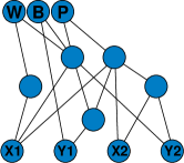
(a) Before Module Mutation

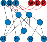
(b) MM(P)

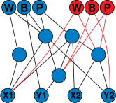
(c) MM(R)

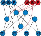
(d) MM(D)

Figure 2: Three Types of Module Mutation. Each form of module mutation provides a different way for evolution to discover how many modules to apply to a problem. LABEL:sub@fig:MMbefore At the start of evolution each CPPN has a single module. LABEL:sub@fig:MMP MM(P) creates a new module with lateral connections from a randomly chosen previous module. The synaptic weight on each lateral connection is $1.0$. The new module’s behavior will depend on the previous module, though activation functions in the new neurons will cause the new module to have slightly different outputs. LABEL:sub@fig:MMR MM(R) creates connections from random source neurons with random synaptic weights leading into the neurons of the new module. The number of incoming connections for each new neuron equals the number of incoming connections to the corresponding neuron of a randomly chosen previous module. LABEL:sub@fig:MMD MM(D) creates a new module that behaves identically to a randomly chosen previous module by creating copies (source neuron and weight) of all incoming connections to that module. Evolution can then cause the behaviors of the duplicated module to diverge through mutations in later generations.

III-C Module Mutation

Module Mutation [8, 4] is any structural mutation operator that adds a new output module to a neural network. An indefinite number of modules may be added in this way. Each network in an initial population starts with a single module, but as evolution progresses, different CPPNs can possess different numbers of modules.

Each application of Module Mutation to a CPPN adds an additional substrate brain to an agent. Each substrate brain possesses a preference neuron. As a result, evolution is discovering which brains to use while also discovering the number of brains each agent should possess.

Several forms of module mutation are used in this paper: MM(P) for Previous, whose new module inputs come directly from a previous output module, MM(R) for Random, whose new module inputs come from random sources in the network, and MM(D) for Duplicate, whose new module inputs are chosen to be the same as those entering another module, thus duplicating the behavior of that module. These approaches are more thoroughly described in Figure 2.

These three new approaches for creating multiple brains for HyperNEAT agents are compared against situational policy geometry and single-brain agents in several domains, which are described next.

IV Experimental Domains

This section reviews two previous multimodal domains and introduces two new ones (Figure 3), which provide a suite of representative tasks to test the new approaches of this paper. These domains all use simulated Khepera robots with rangefinder sensors and three actuators: one each for turning left, turning right, and moving forward. On each time step, the robot will perform whichever of the three actions is most highly activated by the controlling network brain. In some domains, robots also have pie-slice sensors for detecting waypoints. The situation inputs used by situational policy geometry in each domain are also specified. These inputs always depend on a human-specified task division that is also used by the multitask approach. Next, each of these domains are motivated and explained in turn.

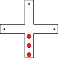
(a) Team Patrol

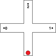
(b) Lone Patrol

(c) Dual Task: Navigation

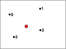
(d) Dual Task: Foraging

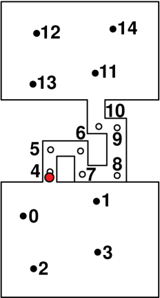
(e) Two Rooms

Figure 3: Domains Requiring Multimodal Behavior. Agents are evolved in four domains. LABEL:sub@fig:teamPatrolDomain Team patrol requires the three robots (red circles) to each visit a different waypoint (black dot) before returning to the start point. LABEL:sub@fig:lonePatrolDomain Lone patrol requires a single robot to visit each waypoint in order before returning. LABEL:sub@fig:dualTaskHallway The first dual task environment is a hallway, which evaluates the robot’s ability to navigate from one end to the other. The same robot is then evaluated in the LABEL:sub@fig:dualTaskForage foraging environment, in which it must visit each waypoint in order. LABEL:sub@fig:twoRoomDomain The two rooms domain combines hallway navigation and foraging. The robot must visit each waypoint in order, clearing the lower room first, and then traversing the hallway before moving on to the upper room. The hollow pellets in the hallway are invisible breadcrumbs that provide incremental fitness benefit for progressing through the hallway, but cannot be perceived by the robot as the waypoints can. In aggregate, these domains feature different types of task divisions, and thus make an interesting test suite of problems to evaluate multimodal methods.

IV-A Team Patrol

The team patrol domain was originally used to demonstrate the effectiveness of situational policy geometry in HyperNEAT [6], and is thus an ideal comparison domain.

The domain is divided into two tasks: advance, in which the three robots spread out to the three segments of a room shaped like a plus sign, and return, in which the robots must return to their original starting positions (Figure 3a). Evaluation lasts 45 seconds, and each second contains 30 time steps. The task switch occurs at the midpoint of the evaluation, regardless of whether the robots reach their individual goals.

Fitness depends both on advancing to the waypoints in each dead end, and on returning home afterward. While advancing, each robot is assigned the closest waypoint as its goal, and while returning the starting point is each robot’s goal. Every second each robot receives a fitness increment equal to the normalized distance from the robot to its goal. In all domains of this paper, the normalized distance is defined as $\frac{D-d}{D}$, where $D$ is the maximum distance for the particular domain, and $d$ is the current distance from the robot to a point of interest.

However, if the robot is within $10$ distance units of its goal, it is considered to have reached it and receives a fitness increment of $1$. To further encourage success, fitness is divided by $10$ if robots do not move after the return signal is given, or if not all waypoints are successfully reached. Furthermore, the fitness for proximity to the starting point is divided by $100$ if the team of robots did not actually reach all way points during the advance stage of evaluation. These specifics are rather complicated, but are taken directly from the original publication that introduced this domain [6].

Robots use six rangefinder sensors tied to substrate inputs. The sensors detect walls but not other robots. In fact, the robots do not physically interact because they are meant to be deployed individually, despite being evaluated simultaneously. Each agent’s substrate also has nine hidden neurons, and three outputs corresponding to the left, forward, and right actions. Because each agent on the team must behave differently, each has its own brain(s). This is accomplished using multi-agent HyperNEAT [31], in which an additional input to the CPPN defines a team dimension along which brains can vary. Each agent is assigned a separate coordinate in this dimension ($-1$, $0$, or $1$).

For situational policy geometry, two separate brains are generated for each agent, through situation inputs of -1 and 1, as described in the example from section II-C. One brain controls the agent during the advancing stage, while the other is used during the retreating stage. When either there is only one brain per agent, or when using preference neurons, a separate situation input is required in the substrates for each brain (at coordinates $(0,-0.8)$). This input tells the brains whether they should currently be advancing or retreating.

IV-B Lone Patrol

Because agents must cooperate to solve the team patrol domain, it conflates the challenges of multiagent coordination and multimodal behavior. Thus, the lone patrol domain is introduced to isolate the multimodal aspect of team patrol.

This goal is accomplished by placing only a single robot in the same environment. This robot is responsible for visiting all branches of the plus sign (Figure 3b). To add to the domain’s challenge, the robot must visit the branches in an order requiring the central four-way intersection to be handled in three different ways: turning left, going straight, and turning right. For situational policy geometry, the situation inputs -1, 0, and 1 correspond to brains for these three behaviors, which switch whenever the agent reaches a waypoint.

The fitness function encourages the robot to reach each of the waypoints as fast as possible in sequence. On every time step fitness is incremented by the normalized distance from the robot to its next goal. However, there is an additional fitness increment of $1$ per waypoint that has already been reached. Therefore, the robot receives increased fitness per time step for reaching additional waypoints. If the robot has visited all waypoints and returned home, the fitness increment is $4$ ($1$ per waypoint) on each remaining time step. Because it takes an individual robot longer to visit all ends of the plus sign, the evaluation time is 80 seconds. though there are still 30 time steps per second.

Both of the domains described so far have subtasks with clear geometrical relationships. Therefore, one might expect situational policy geometry to perform well in these domains. However, many domains have no clear geometrical subdivision. The next domain provides such an example.

IV-C Dual Task

The dual task domain was first introduced to evaluate Evolvable-Substrate HyperNEAT [28], but is appropriated here for testing multimodal approaches. It consists of two isolated tasks, hallway navigation and foraging, where performance and ideal behaviors in each task are unrelated.

In the navigation task (Figure 3c), the robot must navigate from its starting position to the end of a hallway using rangefinder sensors. In the foraging task the robot must visit a sequence of waypoints in order in a rectangular room (Figure 3d). Four pie-slice sensors act as a compass towards each next waypoint.

The agent substrate in this experiment differs from that of the patrol domains, but matches the substrate used in the original experiment [28]. These robots have ten hidden neurons and only five rangefinder inputs. There are also four additional inputs for the pie-slice sensors, which have a y-coordinate of $-1.2$ in the substrate.

Each task has its own fitness function. For the navigation task, fitness is $f_{nav}$, the normalized distance to the goal at the end of evaluation. For the foraging task, fitness is $f_{food}=\frac{n+(1-d_{f})}{4}$, where $n$ is the number of waypoints visited (maximum four) and $d_{f}$ is the normalized distance of the robot to the next waypoint at the end of evaluation. Total fitness is the average of $f_{nav}$ and $f_{food}$.

This fitness function is coarser than those in the patrol domains because it does not matter how quickly the robot reaches its goals. The robot has 45 seconds in each task for a total of 90 seconds per evaluation. However, there are now only five time steps per second.

Because the isolated tasks in this domain have no clear geometric relationship, applying situational policy geometry becomes somewhat arbitrary: the situation inputs are $0$ and $1$ for the hallway and foraging tasks respectively.

While the isolated nature of the tasks in this domain enables clear exploration of the importance of task geometry, subtasks in real world domains are often commingled. Thus the next domain relaxes the constraint of task isolation.

IV-D Two Rooms

The two rooms domain is introduced by this paper. Like the dual task domain, it requires hallway navigation and foraging. However, these tasks are no longer isolated. Instead, two large foraging rooms are separated from each other by a convoluted hallway requiring navigation (Figure 3e).

Each room is filled with waypoints that the robot must visit in order, while the hallway contains invisible breadcrumbs that cannot be sensed, but reward progressing through the hallway. In other words, a breadcrumb is like a waypoint in terms of fitness, but does not register on the robot’s sensors. The robot’s sensors and substrate are the same as in the dual task domain. The pie-slice sensors allow the robot to forage in the rooms, but the rangefinders are crucial for navigating the hallway.

The fitness function for this domain is the same as the dual task’s foraging fitness, except that the total number of waypoints to be visited is 15 (which includes the breadcrumbs in the hallway). Therefore, the fitness is $\frac{n+(1-d_{f})}{15}$, where $d_{f}$ is the normalized distance to the next waypoint at the end of evaluation.

An aspect of this domain that makes it more challenging than dual task is that evaluation ends if the robot collides with a wall. Normal evaluation lasts 200 seconds so the robot has enough time to explore both rooms, and there are 10 time steps per second to give the robot extra maneuverability in the convoluted hallway.

Because this domain integrates hallway navigation and foraging, multitask and situational policy geometry use the following task division: one brain is active when the robot is in the hallway, and another brain is active when it is in one of the two rooms. The situation inputs for these tasks are $0$ for the hallway and $1$ for the rooms.

The experiments described next test how well different approaches to multimodal evolution perform in the four domains described.

V Experimental Setup

In each of the four domains, 30 runs each lasting 2,000 generations were conducted for all approaches. Standard HyperNEAT, which has only one module (1M), provided a performance baseline. The situational policy geometry (SPG) and multitask (MT) approaches had multiple modules reflecting the human-specified task divisions for each domain. Approaches not depending on human-specified task divisions include CPPNs with two (2M) and three (3M) preference modules, and CPPNs that discovered how many modules to use through different forms of module mutation: MM(P), MM(R), or MM(D).

Population sizes differed across domains in order to conform to previous experiments. Team patrol populations had a size of 500 [6], as did lone patrol. The population size for dual task was only 300 [28], as it was also for the two rooms domain.

HyperNEAT parameters were fixed across all experiments. There was a 20% elitist selection rate. Remaining population slots were filled equally by sexual offspring that did not undergo mutation and asexual offspring that had the following rates of mutation: 96% chance of connection weight mutation, 3% chance of connection addition, and 1% chance of node addition. Whenever module mutation was used, it had a 1% chance of occurring. The coefficients for determining species similarity were 1.0 for nodes and connections and 0.1 for weights. The available CPPN activation functions were the sigmoid, Gaussian, absolute value, and sine functions. These parameter settings are the same as in the original team patrol experiment [6].

The experiments in MB-HyperNEAT led to the following results.

VI Results

From a high level, the results show that multimodal approaches discover better behavior faster than 1M, and that multitask and preference neuron approaches can evolve skilled multimodal behavior without any notion of situational policy geometry. Details are presented below.

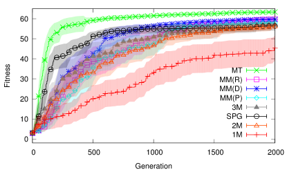
(a) Team Patrol Results

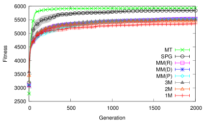
(b) Lone Patrol Results

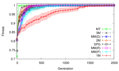
(c) Dual Task Results

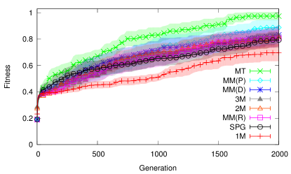
(d) Two Rooms Results

Figure 4: Experimental Results Across Domains. Average champion scores across 30 runs of evolution for each approach are shown across domains. Transparent regions show 95% confidence intervals. The key for each figure lists methods in order of final score, with ties broken according to which method reached the score first. LABEL:sub@fig:teamPatrol In team patrol, MT quickly outperforms all other methods. Preference neuron approaches and SPG plateau around the same lower score, but are all better than 1M. LABEL:sub@fig:lonePatrol In lone patrol, confidence intervals are very narrow, indicating strong convergence across different runs of the same method. MT is still the best, quickly reaching a high plateau. SPG is worse than MT, but better than all preference neuron approaches. Preference neuron approaches cluster together, but are slightly better than 1M. LABEL:sub@fig:dualTask The dual task domain also has narrow confidence intervals. All approaches plateau at the same perfect score, but 1M takes much longer to reach this plateau. MT is still the best, because it reaches the plateau earlier than other approaches. LABEL:sub@fig:twoRoom Modular approaches in the two rooms domain outperform 1M, although there is much overlap in confidence intervals. MM(D), MM(R), 2M, 3M, and SPG cluster together and achieve nearly the same score. MM(P) is slightly better, and is the only method whose final confidence intervals overlap with those of MT, which achieves a much higher score than the other methods. In aggregate, these results show how having multiple brains allows evolved agents to reach better levels of performance faster in domains requiring multimodal behavior.

TABLE I: Adjusted $p$-Values From Pairwise Post-hoc Mann-Whitney $U$ Tests with Bonferroni Error Correction. In each domain, each approach is compared to every other approach using two-tailed Mann-Whitney $U$ tests. In team patrol, lone patrol, and two rooms, fitness scores of champions in the final generation are compared. In dual task, all champions achieve the maximum score, so the numbers of generations taken to reach this score are compared. The $p$-values of each comparison are shown. Note that Bonferroni error correction is used to adjust all $p$-values to prevent spurious detection of statistical differences. Bolded values indicate a significant difference at the $p<0.01$ level while italicized values (two rooms only) are for the $p<0.05$ level. Values using the standard font indicate a lack of a significant difference. Columns and rows in each table are organized from worst to best as in the keys of Figure 4. The conclusion is that MT is the best in each domain while 1M is the worst. There are significant differences between other modular approaches as well.

Team Patrol
	1M	2M	SPG	3M	MM(P)	MM(D)	MM(R)
2M	$\mathbf{0.00091}$	-	-	-	-	-	-
SPG	$\mathbf{6.3\times 10^{-5}}$	1.0	-	-	-	-	-
3M	$\mathbf{3.8\times 10^{-7}}$	1.0	1.0	-	-	-	-
MM(P)	$\mathbf{4.3\times 10^{-10}}$	1.0	1.0	1.0	-	-	-
MM(D)	$\mathbf{1.4\times 10^{-11}}$	$\mathbf{0.00286}$	0.58037	$\mathbf{0.00458}$	0.17764	-	-
MM(R)	$\mathbf{1.4\times 10^{-11}}$	$\mathbf{0.00039}$	0.49246	$\mathbf{0.00458}$	0.12076	1.0	-
MT	$\mathbf{9.5\times 10^{-16}}$	$\mathbf{2.1\times 10^{-10}}$	$\mathbf{4.8\times 10^{-7}}$	$\mathbf{2.6\times 10^{-11}}$	$\mathbf{7.2\times 10^{-10}}$	$\mathbf{0.00013}$	$\mathbf{0.00031}$
Lone Patrol
	1M	2M	3M	MM(P)	MM(D)	MM(R)	SPG
2M	$\mathbf{0.002}$	-	-	-	-	-	-
3M	$\mathbf{1.6\times 10^{-5}}$	0.861	-	-	-	-	-
MM(P)	$\mathbf{8.8\times 10^{-6}}$	0.767	1.0	-	-	-	-
MM(D)	$\mathbf{2.9\times 10^{-6}}$	0.115	1.0	1.0	-	-	-
MM(R)	$\mathbf{3.2\times 10^{-6}}$	0.162	1.0	1.0	1.0	-	-
SPG	$\mathbf{4.7\times 10^{-16}}$	$\mathbf{4.7\times 10^{-16}}$	$\mathbf{4.7\times 10^{-16}}$	$\mathbf{4.7\times 10^{-16}}$	$\mathbf{4.7\times 10^{-16}}$	$\mathbf{9.5\times 10^{-16}}$	-
MT	$\mathbf{4.7\times 10^{-16}}$	$\mathbf{4.7\times 10^{-16}}$	$\mathbf{4.7\times 10^{-16}}$	$\mathbf{4.7\times 10^{-16}}$	$\mathbf{4.7\times 10^{-16}}$	$\mathbf{4.7\times 10^{-16}}$	$\mathbf{5.6\times 10^{-12}}$
Dual Task
	1M	MM(P)	MM(R)	SPG	2M	MM(D)	3M
MM(P)	$\mathbf{0.00104}$	-	-	-	-	-	-
MM(R)	$\mathbf{5.0\times 10^{-5}}$	0.98347	-	-	-	-	-
SPG	$\mathbf{7.5\times 10^{-5}}$	0.91389	1.0	-	-	-	-
2M	$\mathbf{4.7\times 10^{-6}}$	$\mathbf{0.00418}$	0.10761	1.0	-	-	-
MM(D)	$\mathbf{3.9\times 10^{-5}}$	0.60187	1.0	1.0	0.34905	-	-
3M	$\mathbf{1.1\times 10^{-6}}$	$\mathbf{9.1\times 10^{-6}}$	$\mathbf{0.00012}$	0.11535	1.0	$\mathbf{0.00046}$	-
MT	$\mathbf{3.6\times 10^{-8}}$	$\mathbf{5.2\times 10^{-9}}$	$\mathbf{6.6\times 10^{-9}}$	$\mathbf{8.7\times 10^{-6}}$	$\mathbf{0.00308}$	$\mathbf{8.4\times 10^{-9}}$	$\mathbf{0.00627}$
Two Rooms
	1M	SPG	MM(R)	2M	3M	MM(D)	MM(P)
SPG	$\mathit{0.04858}$	-	-	-	-	-	-
MM(R)	0.41388	1.0	-	-	-	-	-
2M	0.07329	1.0	1.0	-	-	-	-
3M	0.10012	1.0	1.0	1.0	-	-	-
MM(D)	0.08861	1.0	1.0	1.0	1.0	-	-
MM(P)	$\mathbf{0.00217}$	1.0	1.0	1.0	1.0	1.0	-
MT	$\mathbf{7.7\times 10^{-7}}$	$\mathbf{0.0002}$	$\mathbf{0.00067}$	$\mathbf{0.00121}$	$\mathit{0.01137}$	$\mathbf{0.00366}$	0.3591

VI-A Team Patrol Results

Aligning with previous studies in this domain, SPG outperforms 1M. However, MT outperforms SPG, and preference neuron approaches eventually reach scores around or slightly above those of SPG (Figure 4a).

In the final generation, the Kruskal-Wallis test indicates a significant difference between champion fitness scores of different approaches ($H=117.7784,df=7,N=30,p<2.2\times 10^{-16}$). Post-hoc tests indicate that all modular approaches significantly outperform 1M, and MT significantly outperforms all other methods. These differences and differences between some preference neuron methods are reported in Table I.

Observation of evolved behaviors reveals qualitative differences between methods. The behavior of MT networks involves each robot going directly to its destination and returning in perfect synchronicity. Less skilled modular networks will generally have small inefficiencies, such as one out of the three robots lagging slightly behind the others. In the worst runs, one of the robots becomes stuck advancing outward and fails to return. Such failure is common in 1M runs, but happens to some preference neuron champions as well. Videos of several representative behaviors are at southwestern.edu/~schrum2/re/team-patrol.html.

These videos also reveal how preference neuron approaches switch between brains. Interestingly, different team members switch brains at different times. Some robots use a single brain for advancing and returning, while others in the same team frequently switch brains. Most common is to rely on one brain to advance, switch to turn around once the signal input activates, and then switch back to the original brain to return home.

Module mutation champions produce many unused brains. Some have between 10 and 20 substrate brains, but agents use no more than three of them. This result occurs in the other domains as well.

VI-B Lone Patrol Results

Results in the lone patrol domain have little variation; runs of each method quickly converge (Figure 4b). MT performs best, followed by SPG, then all preference neuron methods (which cluster together), and finally 1M, which performs worst.

The Kruskal-Wallis test again indicates significant differences between final champion scores in this domain ($H=162.3146,df=7,N=30,p<2.2\times 10^{-16}$). In fact, post-hoc tests indicate that all methods are significantly different from each other, except methods that use preference neurons (Table I). Specifically, 2M, 3M, MM(P), MM(R), and MM(D) are not significantly different from each other, but are different from the other methods.

Videos of evolved behavior show that most champions reach or nearly reach all waypoints. Fitness score differences depend on route efficiency. Preference neuron approaches and 1M perform worse because some champions become stuck on a corner when returning home after visiting the final waypoint. Representative videos can be viewed at southwestern.edu/~schrum2/re/lone-patrol.html.

MT performs well because it proceeds directly to each waypoint and promptly turns to the next waypoint once the preceding one is reached. SPG generally does the same, but sometimes goes around corners less efficiently than MT. Preference neuron networks often waste time at each end of the plus sign and when turning corners. They often proceed to the end of each hallway rather than turning around directly as each waypoint is reached (they do not sense when they reach each waypoint), and often move around corners in discontinuous starts and stops rather than in a continuous arc. Dealing with turns generally requires dedicated brains. Specifically, turning around at each dead end is often assigned a dedicated brain, and there is often a brain dedicated to handling turning in the plus’s center. Sometimes turning is accomplished by thrashing between the dedicated turning brain and whatever brain was being used previously. These behaviors typically require the use of three brains, though module mutation frequently produces CPPNs with 10 or more modules, whose brains are mostly unused.

Deciding on actions when at the center of the plus sign provides a challenge for the robot, because it looks the same to the robot’s sensors on each visit (the domain is partially observable [32]), yet each visit a different behavior is needed. The 1M networks perform the worst because even when they successfully visit all waypoints and return home, they tend to navigate the plus sign’s center with an inefficient trick. Instead of turning right, the robot loops around by turning left repeatedly. The added time required to perform this maneuver has a large fitness cost.

Both patrol domains have fitness functions that not only reward reaching certain goals, but doing so quickly. Distinctions between methods in lone patrol depend more on how quickly all waypoints are visited than on whether they are reached. However, the fitness functions for the next two domains only measure whether or not the robot ever achieves its goals, irrespective of speed.

VI-C Dual Task Results

All methods eventually master the dual task, obtaining a perfect fitness (Figure 4c). However, there are distinctions in how many generations each method requires to succeed. MT is still the best, succeeding in less than 100 generations in all runs. SPG and the preference neuron methods take slightly longer to reach maximum fitness, while 1M takes significantly longer.

Because all runs achieve maximum fitness, the Kruskal-Wallis test is applied to the number of generations necessary to succeed in this way, and indicates a significant difference ($H=114.2459,df=7,N=30,p<2.2\times 10^{-16}$). Post-hoc tests indicate that all other methods succeed significantly faster than 1M, and MT succeeds significantly faster than all other methods. These differences and others are reported in Table I.

Although all methods eventually achieve perfect fitness, there are many examples of inefficient behavior, because there is no selection for efficiency. Thus, many champions collide with walls in the hallway task or become stuck for long periods. There is less time for mistakes in the foraging task, so performance in this task is relatively straightforward: robots go directly to each waypoint in sequence. Example behaviors can be seen at southwestern.edu/~schrum2/re/dual-task.html.

Preference neuron approaches actively use at most three brains. Instead of dedicating separate brains to individual tasks, as in MT and SPG, the same set of brains is repurposed across tasks. In the hallway task, it is common for one brain to handle moving straight forward, while one or two others handle turning around corners. In the foraging task it is common to have one brain that moves straight toward the next waypoint, while another brain takes over to turn the robot around after each waypoint is reached.

Although these usage patterns are common, there are also module mutation champions that have nearly 20 brains, yet solve both tasks using only one. Many module mutation champions use two or three brains instead, but also leave many brains unused.

The next domain, which is closely related to this one, nevertheless produces very different results, as shown next.

VI-D Two Rooms Results

As in the other domains, MT performs best in two rooms, although its margin of success is not as dramatic (Figure 4d). The 1M approach is once again the worst, with SPG and preference neuron approaches clustering between 1M and MT.

Because no method succeeds in all runs, the Kruskal-Wallis test is again applied to fitness scores of the final champions, and indicates that there are significant differences between methods ($H=43.9804,df=7,N=30,p\approx 2.156\times 10^{-7}$). Post-hoc tests indicate that although 1M has the lowest final scores, it is only significantly outperformed by SPG, MM(P) and MT. MT significantly outperforms all methods, except MM(P) (Table I).

The worst-performing champions visit all waypoints in the first room, but fail to progress through the hallway. There are also slightly more successful robots that use foraging behavior so inefficient that they cannot visit all waypoints in the second room within the time limit, despite successfully navigating the hallway. Examples of inefficient behavior include heading toward each waypoint in tight spirals instead of in a straight line, and circling the wall of the first room to find the hallway instead of directly heading to it. This range of behaviors explains the broad dispersion of champion fitness scores. Videos of representative behaviors can be seen at southwestern.edu/~schrum2/re/two-rooms.html.

When preference neurons are used, often one brain is mostly responsible for navigating the hallway. However, this brain will typically alternate rapidly with whatever brain was previously active. Visiting waypoints in each room is generally handled by a single brain, though sometimes another brain activates to reorient the robot after each waypoint is reached (as in the foraging environment of the dual task). These types of behaviors seldom require more than two or three brains, and once again many module mutation runs produce many unnecessary brains.

Interestingly, while MT performs best, the decision to dedicate a brain to hallway navigation requires human insight. However, SPG performs poorly despite using the same task division, thus providing a clear example of how constraining different controllers to be geometrically related can be harmful.

VII Discussion and Future Work

All multi-brain approaches to creating agents are superior to 1M in at least three of the four explored domains. SPG is superior to 1M in all domains, but also inferior to MT in all domains, thus demonstrating that even in domains where situational policy geometry seems appropriate, it is better to allow a multitask CPPN to create completely distinct brains instead. For this reason, if a human-specified task division is available, multitask CPPNs seem the most principled first approach.

However, preference neuron approaches can be applied even when a task division is not available, and at least one preference neuron approach is significantly better than 1M in each domain. However, because effective task divisions were available, preference neurons are never significantly better than SPG, and are inferior to MT. This result contrasts with previous results in Ms. Pac-Man using the direct encoding MM-NEAT [4, 17]. It is possible that preference neurons are less effective when combined with HyperNEAT than with directly encoded neural networks, but it is more likely that the increased complexity of Ms. Pac-Man (compared to the domains of this paper) is what allowed preference neurons to shine. Therefore, applying MB-HyperNEAT to more complex domains lacking a clear task division is one avenue of future work.

There is no consistent relationship between the performance of a fixed number of preference neuron brains (2M and 3M) and variants of module mutation. In team patrol, module mutation outperforms a fixed number of brains, but this relation is reversed in dual task. In lone patrol, all preference neuron approaches perform equivalently, as is the case in two rooms (even though MM(P) significantly outperforms 1M). Distinctions between different forms of module mutation form no consistent pattern either.

Even when there are statistically significant differences between preference neuron approaches, the effect size is small. Observing how many brains are actually used in each domain provides an explanation: regardless of how many brains module mutation produces, the final champions only use one to three of them. Therefore, it makes sense that the behaviors exhibited and fitness scores achieved by module mutation are similar to those of a set number of preference neuron brains. Given the performance of MT in all domains, it is clear that two to three brains are sufficient, if they are used correctly. A domain complex enough to either require more than three modules, or one lacking an obvious human-specified task division, is likely required for module mutation to show practical benefit over simpler methods.

It is unclear how the many unused controllers produced by module mutation affect evolution. Why do certain forms of module mutation sometimes do better than approaches with a set number of preference neuron brains despite producing champions that use the same number of brains? Intuitively, wasting mutation operations on CPPN modules which only affect brains that are never used seems like it would slow down evolution. Selection cannot act on unused modules. These portions of the CPPN are effectively introns, a biological phenomenon that is also known in the Genetic Programming community [33].

An intron is a gene that does not affect the phenotype. In general, introns can be safely modified without changing a genotype’s fitness. Therefore, genotypes that already have high fitness are more likely to persist in the population, because introns make them less vulnerable to destructive mutations by providing a portion of the genotype that can be changed without effect. With regard to module mutation specifically, there is also a chance that mutations in an intron could cause long unused modules to suddenly start being used. Such modules will likely hurt fitness in most cases because they have not been subject to any selection pressure. However, the sudden emergence of a good module could help a population escape a local optimum in the fitness landscape. The few cases where such positive mutations occur could be enough to make module mutation beneficial overall, at least in certain domains. The performance of MM(P) in two rooms is an example.

This paper generated multimodal behavior by creating several complete brains in separate substrates. However, HyperNEAT can also take advantage of multiple sensory modalities using a multi-spatial substrate (MSS [30]), which can embed the neurons of a single brain into several sub-substrates. Different modalities of input are separated into different substrates that are integrated by a hidden layer substrate, which eventually propagates to a final output substrate. The MSS approach could be compared against, and even combined with the methods of this paper in future work.

Another focus for future work is the evolution of larger networks. One of the primary benefits of HyperNEAT is its ability to compactly encode large networks [9, 10, 11], so it is important to verify that the HyperNEAT extensions presented in this paper also provide a benefit to the large, complex networks that HyperNEAT was designed to create.

VIII Conclusion

Automatic and effective evolution of complex multimodal behavior requires indirect encodings and mechanisms that support evolving distinct neural structures. The main idea in this paper is to combine the popular HyperNEAT indirect encoding and the MM-NEAT approach to evolving modular networks, thereby realizing the strengths of both approaches. The result is MB-HyperNEAT, a collection of methods for creating multiple brains for a single agent. Results show that the multitask CPPN approach always outperforms a previous attempt to merge HyperNEAT with multimodal extensions known as situational policy geometry, and that approaches using preference neurons make it possible to evolve agents with multiple brains when a human-specified task division is unavailable. Preference neuron approaches achieve lower scores than multitask CPPNs, but even though they are not provided with a human-specified task division, their scores are often statistically tied with those of situational policy geometry, and generally surpass scores of agents with only one brain. The conclusion is that MB-HyperNEAT is a promising toolkit for evolving complex multimodal behavior that can reduce the need for specialized domain knowledge.

References

- [1] K. O. Stanley and R. Miikkulainen, “Evolving Neural Networks Through Augmenting Topologies,” Evolutionary Computation Journal, vol. 10, pp. 99–127, 2002.
- [2] D. Floreano, P. Dürr, and C. Mattiussi, “Neuroevolution: From Architectures to Learning,” Evolutionary Intelligence, vol. 1, no. 1, pp. 47–62, 2008.
- [3] R. Calabretta, S. Nolfi, D. Parisi, and G. Wagner, “Duplication of Modules Facilitates the Evolution of Functional Specialization,” Artificial Life, vol. 6, no. 1, pp. 69–84, 2000.
- [4] J. Schrum and R. Miikkulainen, “Discovering Multimodal Behavior in Ms. Pac-Man through Evolution of Modular Neural Networks,” TCIAIG, vol. 8, no. 1, pp. 67–81, 2016. [Online]. Available: http://nn.cs.utexas.edu/?schrum:tciaig16
- [5] K. O. Stanley, D. B. D’Ambrosio, and J. Gauci, “A Hypercube-based Encoding for Evolving Large-scale Neural Networks,” Artificial Life, vol. 15, no. 2, pp. 185–212, Apr. 2009. [Online]. Available: http://dx.doi.org/10.1162/artl.2009.15.2.15202
- [6] D. B. D’Ambrosio, J. Lehman, S. Risi, and K. O. Stanley, “Task Switching in Multirobot Learning Through Indirect Encoding,” in International Conference on Intelligent Robots and Systems. IEEE, 2011, pp. 2802–2809.
- [7] J. Schrum and R. Miikkulainen, “Evolving Multimodal Behavior With Modular Neural Networks in Ms. Pac-Man,” in Genetic and Evolutionary Computation Conference. ACM, July 2014, pp. 325–332. [Online]. Available: http://nn.cs.utexas.edu/?schrum:gecco2014
- [8] ——, “Evolving Multimodal Networks for Multitask Games,” IEEE Transactions on Computational Intelligence and AI in Games, vol. 4, no. 2, pp. 94–111, June 2012. [Online]. Available: http://nn.cs.utexas.edu/?schrum:tciaig12
- [9] M. Hausknecht, J. Lehman, R. Miikkulainen, and P. Stone, “A Neuroevolution Approach to General Atari Game Playing,” IEEE Transactions on Computational Intelligence and AI in Games, vol. 6, no. 4, pp. 355–366, Dec 2014. [Online]. Available: http://nn.cs.utexas.edu/?hausknecht:tciaig14
- [10] J. Gauci and K. O. Stanley, “A Case Study on the Critical Role of Geometric Regularity in Machine Learning,” in National Conference on Artificial Intelligence (AAAI-08). AAAI Press, 2008, pp. 628–633.
- [11] ——, Parallel Problem Solving from Nature. Berlin, Heidelberg: Springer Berlin Heidelberg, 2010, ch. Indirect Encoding of Neural Networks for Scalable Go, pp. 354–363. [Online]. Available: http://dx.doi.org/10.1007/978-3-642-15844-5_36
- [12] S. Haykin, Neural Networks, A Comprehensive Foundation. Upper Saddle River, New Jersey: Prentice Hall, 1999.
- [13] N. Kashtan and U. Alon, “Spontaneous Evolution of Modularity and Network Motifs,” National Academy of Sciences USA, vol. 102, no. 39, pp. 13 773–13 778, 2005.
- [14] J. Clune, J.-B. Mouret, and H. Lipson, “The Evolutionary Origins of Modularity,” Royal Society B: Biological Sciences, vol. 280, no. 1755, pp. 20 122 863–20 122 863, 2013.
- [15] J. Huizinga, J.-B. Mouret, and J. Clune, “Evolving Neural Networks That Are Both Modular and Regular: HyperNEAT Plus the Connection Cost Technique,” in Genetic and Evolutionary Computation Conference. ACM, July 2014, pp. 697–704.
- [16] S. Nolfi, “Using Emergent Modularity to Develop Control Systems for Mobile Robots,” Adaptive Behavior, vol. 5, pp. 343–363, 1996.
- [17] J. Schrum and R. Miikkulainen, “Solving Interleaved and Blended Sequential Decision-Making Problems through Modular Neuroevolution,” in Genetic and Evolutionary Computation Conference. ACM, July 2015, pp. 345–352. [Online]. Available: http://nn.cs.utexas.edu/?schrum:gecco2015
- [18] G. Howard, L. Bull, and P.-L. Lanzi, “A Spiking Neural Representation for XCSF,” in Congress on Evolutionary Computation. IEEE, 2010, pp. 1–8.
- [19] J. Hurst and L. Bull, “A Neural Learning Classifier System with Self-Adaptive Constructivism for Mobile Robot Control,” Artificial Life, vol. 12, no. 3, pp. 353–380, 2006. [Online]. Available: http://dx.doi.org/10.1162/artl.2006.12.3.353
- [20] H. H. Dam, H. A. Abbass, and C. Lokan, “Neural-based learning classifier systems,” IEEE Transactions on Knowledge and Data Engineering, vol. 20, no. 1, pp. 26–39, 2008. [Online]. Available: http://ieeexplore.ieee.org/lpdocs/epic03/wrapper.htm?arnumber=4358957
- [21] J. Togelius, “Evolution of a Subsumption Architecture Neurocontroller,” Intelligent and Fuzzy Systems, pp. 15–20, 2004.
- [22] T. Thompson, F. Milne, A. Andrew, and J. Levine, “Improving Control Through Subsumption in the EvoTanks Domain,” in Conference on Computational Intelligence and Games. IEEE, 2009, pp. 363–370.
- [23] N. van Hoorn, J. Togelius, and J. Schmidhuber, “Hierarchical Controller Learning in a First-Person Shooter,” in Conference on Computational Intelligence and Games. IEEE, 2009, pp. 294–301.
- [24] D. Lessin, D. Fussell, and R. Miikkulainen, “Open-Ended Behavioral Complexity for Evolved Virtual Creatures,” in Genetic and Evolutionary Computation Conference. ACM, 2013, pp. 335–342. [Online]. Available: http://nn.cs.utexas.edu/?lessin:gecco13
- [25] ——, “Adapting Morphology to Multiple Tasks in Evolved Virtual Creatures,” in International Conference on the Synthesis and Simulation of Living Systems (ALIFE 14), 2014. [Online]. Available: http://nn.cs.utexas.edu/?lessin:alife14
- [26] R. A. Caruana, “Multitask Learning: A Knowledge-based Source of Inductive Bias,” in International Conference on Machine Learning, 1993, pp. 41–48.
- [27] J. Secretan, N. Beato, D. B. D’Ambrosio, A. Rodriguez, A. Campbell, J. T. Folsom-Kovarik, and K. O. Stanley, “Picbreeder: A Case Study in Collaborative Evolutionary Exploration of Design Space,” Evolutionary Computation, vol. 19, no. 3, pp. 373–403, Sep. 2011. [Online]. Available: http://dx.doi.org/10.1162/EVCO_a_00030
- [28] S. Risi and K. O. Stanley, “An Enhanced Hypercube-Based Encoding for Evolving the Placement, Density and Connectivity of Neurons,” Artificial Life, vol. 18, no. 4, pp. 331–363, 2012.
- [29] J. Drchal, O. Kaprál, J. Koutník, and M. Šnorek, “Combining Multiple Inputs in HyperNEAT Mobile Agent Controller,” in International Conference on Artificial Neural Networks, Part II, vol. 2. Berlin: Springer, 2009, pp. 775–783.
- [30] J. K. Pugh and K. O. Stanley, “Evolving Multimodal Controllers with HyperNEAT,” in Genetic and Evolutionary Computation Conference. ACM, 2013, pp. 735–742. [Online]. Available: http://doi.acm.org/10.1145/2463372.2463459
- [31] D. B. D’Ambrosio, J. Lehman, S. Risi, and K. O. Stanley, “Evolving Policy Geometry for Scalable Multiagent Learning,” in Proceedings of the International Conference on Autonomous Agents and Multiagent Systems (AAMAS), 2010, pp. 731–738.
- [32] L. P. Kaelbling, M. L. Littman, and A. R. Cassandra, “Planning and Acting in Partially Observable Stochastic Domains,” Artificial intelligence, vol. 101, no. 1, pp. 99–134, 1998.
- [33] P. Nordin, F. Francone, and W. Banzhaf, “Explicitly Defined Introns and Destructive Crossover in Genetic Programming,” in Advances in Genetic Programming. MIT Press, 1996, pp. 111–134. [Online]. Available: http://dl.acm.org/citation.cfm?id=270195.270205