A first order Tsallis theory

Abstract

We investigate first-order approximations to both i) Tsallis’ entropy $S_{q}$ and ii) the $S_{q}$-MaxEnt solution (called q-exponential functions $e_{q}$). We use an approximation/expansion for $q$ very close to unity. It is shown that the functions arising from the procedure ii) are the MaxEnt solutions to the entropy emerging from i). The present treatment is free of the poles that, for classic quadratic Hamiltonians, appear in Tsallis’ approach, as demonstrated in [Europhysics Letters 104, (2013), 60003]. Additionally, we show that our treatment is compatible with extant date on the ozone layer.

Keywords: MaxEnt, second variation, generalized statistics. Tsallis entropy, divergences, partition function, specific heat.

1 Introduction

During the last quarter of century, an active subfield of statistical mechanics is centered around the concept of the so-called q-statistics, that Tsallis introduced in [1, 2], that appears to yield better answers, in many scenarios, than the orthodox Boltzmann-Gibbs entropic functional [3]. These scenarios involve variegated disciplines (see, for instance, [4]-[5], [6], [7], [8], [9], [10], [11], [12], [13], [14], [15], [18], etc.) Concepts involving q-statistics are important not only in physics but in chemistry, biology, mathematics, economics, and informatics as well [19], [20].

In this work we revisit the Tsallis-subject by appealing to perturbation theory around $q=1$. We investigate first-order approximations to both A) Tsallis’ entropy $S_{q}$ and B) the $S_{q}$-MaxEnt solution (called q-exponential functions $e_{q}$). It is shown that the functions arising from the procedure B) are the MaxEnt solutions to the entropy emerging from A). The present treatment is free of the poles that, for classic quadratic Hamiltonians, plague Tsallis’ approach, as demonstrated in [21]. Additionally, we show that our treatment is compatible with extant date on the ozone layer [24, 25, 26].

1.1 Motivation

It was shown in [27] that data-detection following a normalization step does not permit straightforward inference of data-distribution in exponential or Gaussian fashion because of a systematic transformation into $q-$exponentials or q-Gaussians. The origin of the often encountered $q-$exponential or q-Gaussian data needs careful analysis. For a very large set of recorded-data (elliptical ones), this occurrence is a simple consequence of a device-normalization stage [27]. This entails that the q-neighborhood of $q=1$ is extremely important for q-statistics, deserving the special attention that it receives below.

Note also that in the superstatistics approach of Beck and Cohen [28], the parameter $q-1$ is a measure of temperature fluctuations in the driven nonequilibrium system with a stationary state, so small $q-1$ corresponds to sharply peaked temperature distributions around the mean.

2 Still another new entropy

After the pioneer Tsallis’ paper [2], many new entropies have been proposed [29]. In this vein, we begin our considerations with reference to a new q-entropy, that exhibits over Tsallis’ one some important advantages to be discussed below. The new entropy will emerge as a result of a the first order approximation (around $q=1$) of the q-exponential function [3]:

$$[1+(1-q)\beta U]^{\frac{1}{q-1}}\simeq\left[1+\frac{(1-q)}{2}\beta^{2}U^{2}\right]e^{-\beta U}.$$ (2.1)

The pertinent probability distribution becomes now, instead of the q-exponential [3], the following one

$$P=\frac{\left[1+\frac{(1-q)}{2}\beta^{2}U^{2}\right]e^{-\beta U}}{{\cal Z}},$$ (2.2)

with

$${\cal Z}=\int\limits_{M}\left[1+\frac{(1-q)}{2}\beta^{2}U^{2}\right]e^{-\beta U}d\mu.$$ (2.3)

We construct next the first order approximation to Tsallis’ entropy [3] and find

$${\cal S}_{q}=\frac{1}{1-q}\left(1-\int\limits_{M}P^{q}d\mu\right)\simeq-\int\limits_{M}P\ln P\left[1+\frac{(q-1)}{2}\ln P\right]d\mu.$$ (2.4)

We show next (2.2) arises from extremizing (2.4). The ensuing variational problem revolves around a Lagrangian

$${\cal F}_{{\cal S}_{q}}(P)=-\int\limits_{M}P\ln P\left[1+\frac{(q-1)}{2}\ln P\right]d\mu+\lambda_{1}\left(\int\limits_{M}PUd\mu-<U>\right)+$$

$$\lambda_{2}\left(\int\limits_{M}Pd\mu-1\right),$$ (2.5)

whose increment is

$${\cal F}_{{\cal S}_{q}}(P+h)=-\int\limits_{M}(P+h)\ln(P+h)\left[1+\frac{(q-1)}{2}\ln(P+h)\right]d\mu+$$

$$\lambda_{1}\left(\int\limits_{M}(P+h)Ud\mu-<U>\right)+\lambda_{2}\left(\int\limits_{M}(P+h)d\mu-1\right),$$ (2.6)

so that

$${\cal F}_{{\cal S}_{q}}(P+h)-{\cal F}_{{\cal S}_{q}}(P)=-\int\limits_{M}(P+h)\ln(P+h)\left[1+\frac{(q-1)}{2}\ln(P+h)\right]d\mu+$$

$$\int\limits_{M}P\ln P\left[1+\frac{(q-1)}{2}\ln P\right]d\mu+\lambda_{1}\int\limits_{M}Uhd\mu+\lambda_{2}\int\limits_{M}hd\mu,$$ (2.7)

or

$${\cal F}_{{\cal S}_{q}}(P+h)-{\cal F}_{{\cal S}_{q}}(P)=-\int\limits_{M}\left[1+\ln P+\left(\frac{q-1}{2}\right)\left(2\ln P+\ln^{2}P\right)-\lambda_{1}-\lambda_{2}\right]hd\mu$$

$$-\int\limits_{M}\left[\frac{1}{2P}+\left(\frac{q-1}{2}\right)\left(\frac{1+\ln P}{P}\right)\right]h^{2}d\mu.$$ (2.8)

The last relation yields the extremizing distribution $P$

$$1+\ln P+\left(\frac{q-1}{2}\right)\left(2\ln P+\ln^{2}P\right)-\lambda_{1}-\lambda_{2}=0$$ (2.9)

$$-\int\limits_{M}\left[\frac{1}{P}+\left(q-1\right)\left(\frac{1+\ln P}{P}\right)\right]h^{2}d\mu\leq C||h||^{2},$$ (2.10)

with $C<0$ is a constant. See [22], [23]. Replacing (2.2) into (2.9) one verifies that $P$ is a solution to (2.9), with $\lambda_{1}$ and $\lambda_{2}$ given by

$$\lambda_{1}=-\beta[q-(q-1)\ln{\cal Z}]$$ (2.11)

$$\lambda_{2}=1-q\ln{\cal Z}+\left(\frac{q-1}{2}\right)\ln^{2}{\cal Z}$$ (2.12)

Of course, (2.10) must be verified for a maximum.

We realize that the entropy (2.4) is not just an approximation but a legitimate new thermodynamic one, since it complies with the MaxEnt strictures.

2.1 Comparison between the exact and approximate solutions

Figs. 1,2,3, and 4 correspond to the modulus of the ratio between the approximate and the exact solutions (AER), eq. (2.1). Horizontal coordinates are in meters. For simplicity we have taken $U=x^{2}$ and $\beta=1$. The agreement is excellent. More to the point, it is excellent over extremely long distances, for atomic phenomena.

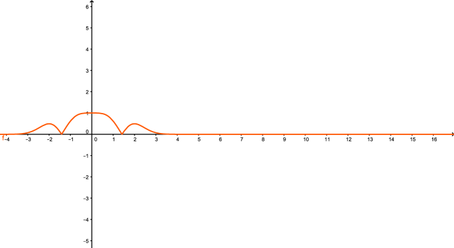
Figure 1: AER (see text) for $1-q=0.5$

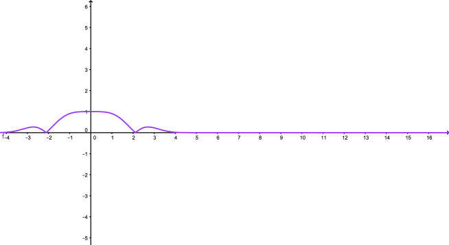
Figure 2: AER (see text) for $1-q=0.1$

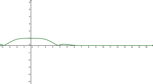
Figure 3: AER (see text) for $1-q=0.01$

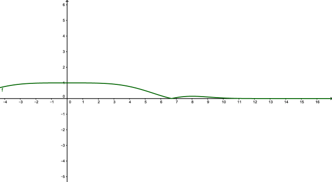
Figure 4: AER (see text) for $1-q=0.001$

3 Quadratic Hamiltonians

3.1 Review of Tsallis’ treatment

In reference [21] one finds the associated partition function and mean energy for Tsallis’ q-MaxEnt approach, i.e.,

$${\cal Z}=\frac{\pi^{\nu}}{\Gamma(\nu)}\int\limits_{0}^{\infty}\frac{u^{\nu-1}}{[1+\beta(q-1)u]^{\frac{1}{q-1}}}du,$$ (3.1)

where the integral is evaluated using [30]:

$${\cal Z}=\frac{\pi^{\nu}}{[\beta(q-1)]^{\nu}}\frac{\Gamma\left(\frac{1}{q-1}-\nu\right)}{\Gamma\left(\frac{1}{q-1}\right)}.$$ (3.2)

This result is valid for $q\neq 1$ and we have selected $1\leq q<2$. Of course, $q=1$ is the orthodox result, for which the q-exponential transforms itself into the ordinary exponential function (and the integral (3.1) is convergent). The singularities (divergences) of (3.1) are, of course, given by the poles of the $\Gamma$ function, that is, for

$$\frac{1}{q-1}-\nu=-p\;\;{\rm for}\;\;p=0,1,2,3,......,$$

i.e., $q-$ values given by

$$q=\frac{3}{2},\frac{4}{3},\frac{5}{4},\frac{6}{5},......,\frac{\nu}{\nu-1},\frac{\nu+1}{\nu}$$

For the mean enrgy, instead, (3.1) gives

$$<{\cal U}>=\frac{\pi^{\nu}}{\Gamma(\nu){\cal Z}}\int\limits_{0}^{\infty}\frac{u^{\nu}}{[1+\beta(q-1)u]^{\frac{1}{q-1}}}du,$$ (3.3)

so that, using [30] one finds

$$<{\cal U}>=\frac{\nu\pi^{\nu}}{{\cal Z}[\beta(q-1)]^{\nu+1}}\frac{\Gamma\left(\frac{1}{q-1}-\nu-1\right)}{\Gamma\left(\frac{1}{q-1}\right)},$$ (3.4)

Here, the poles are given by

$$\frac{1}{q-1}-\nu-1=-p\;\;\;{\rm for}\;p=0,1,2,3,......,$$

or,

$$q=\frac{3}{2},\frac{4}{3},\frac{5}{4},\frac{6}{5},......,\frac{\nu+1}{\nu},\frac{\nu+2}{\nu+1}.$$

As customary [31], using q-logarithms [2] $\ln_{q}(x)=\frac{x^{1-q}-1}{1-q}$, Tsallis’ entropy becomes

$${\cal S}_{q}=\ln_{q}{\cal Z}+{\cal Z}^{1-q}\beta<{\cal U}>,$$ (3.5)

that is finite if ${\cal Z}$ and $<{\cal U}>$ are also finite.

3.2 The new entropy alternative

The new partition function is easily seen to be

$${\cal Z}=\frac{\pi^{\nu}}{\Gamma(\nu)}\int\limits_{0}^{\infty}u^{\nu-1}\left[1+\frac{(q-1)}{2}\beta^{2}u^{2}\right]e^{-\beta u}du,$$ (3.1)

and, evaluating the integral,

$${\cal Z}=\frac{\pi^{\nu}}{\beta^{\nu}}\left[1+\frac{(q-1)\nu(\nu+1)}{2}\right].$$ (3.2)

No poles are detected! For $q=1$ this yields the Boltzmann-Gibbs’ (BG) partition function. For the mean energy one has

$$<{\cal U}>=\frac{\pi^{\nu}}{\Gamma(\nu){\cal Z}}\int\limits_{0}^{\infty}u^{\nu}\left[1+\frac{(q-1)}{2}\beta^{2}u^{2}\right]e^{-\beta u}du,$$ (3.3)

and after integration

$$<{\cal U}>=\frac{\nu\pi^{\nu}}{\beta^{\nu+1}{\cal Z}}\left[1+\frac{(q-1)}{2}(\nu+1)(\nu+2)\right],$$ (3.4)

with, again, no poles. Using now (3.2) we obtain

$$<{\cal U}>=\frac{\nu}{\beta}\left[1+(q-1)(\nu+1)\right],$$ (3.5)

that coincides with the BG result for $q=1$. As for the entropy, one must develop up to first order ${\cal Z}^{1-q}$ and we get

$${\cal Z}^{1-q}=1+(q-1)\nu\ln\left(\frac{\beta}{\pi}\right)+\frac{(q-1)^{2}}{2}\left[\nu^{2}\ln^{2}\left(\frac{\beta}{\pi}\right)-\nu(\nu+1)\right],$$ (3.6)

that together with (3.5) leads to

$${\cal S}_{q}=\nu\left[1+\ln\left(\frac{\beta}{\pi}\right)\right]+(q-1)\left[\nu+1-\frac{\nu(\nu+1)}{2}+\nu\ln\left(\frac{\beta}{\pi}\right)-\frac{\nu^{2}}{2}\ln^{2}\left(\frac{\beta}{\pi}\right)\right],$$ (3.7)

that for $q=1$ is the BG result.

3.3 Specific Heat

We need the derivative of (3.5) with respect to the temperature $T$ to reach

$${\cal C}=\nu{\cal K}\left[1+(q-1)(\nu+1)\right],$$ (3.1)

with ${\cal K}$ Boltzmann’s constant. For $q=1$ we reobtain the BG result. The corrections in 3.1 to the BG could easily be checked out empirically.

4 The Ozone layer

Tsallis’ $q-$triplet [25] is possibly the most spectacular empirical quantifier of non-extensivity, i.e., $q\neq 1$. The quantifier was studied in [26] with reference to an experimental time-series related to the daily depth-values of the stratospheric ozone layer. Pertinent data were there expressed in Dobson units and ranged from 1978 till 2005. After evaluation of the three associated Tsallis’ q-indexes one concluded that nonextensivity is clearly a characteristic of the ozone layer.

Stratospheric ozone is encountered mainly within a $\sim 15$km-layer at a height of about 15km. There is a low density of a few $O_{3}-$molecules per million of air-molecules. The associated mechanism of interactions responsible for depletion is given in Ref. [24]. A stationary regime prevails, modulated by various types of oscillations, that is 1) a yearly one due to the orientation of the incoming radiation, 2) other of a period of around 2 years originated in stratospheric air-currents, and 3) a secular variation [24]. In [26] the authors concentrated efforts on two time-series: A) $\{Z_{n}\}$ of depth-values for the ozone layer and B) its daily variability $\{\Delta Z_{n}\}$.

Tsallis’ theory displays three important q-features (three different q-values) [25]:

• i) A q-value linked to meta-stable states, the one of the pertinent $q$-exponential, that we call $q\equiv q_{stat}$.

• ii) The above states display a $q$-exponential sensibility to initial conditions (the so-called weak chaos). We speak of a q-value that we call $q_{sens}$.

• iii) Meta-stable macroscopic quantities relax to their $q=1$-values in a $q$-exponential fashion with $q=q_{rel}$.

Thus, a meta-stable state is characterized by a triplet of $q-$values: $(q-{stat},q-{sens},q-{rel})\neq(1,1,1)$, where $q-{stat}>1$, $q-{sen}<1$, and $q-{rel}>1$ [25].

Since in the case of the BG statistics the three different q-values above coalesce to $q=1$, with the present treatment we expect a convergence of the three triplet’s q-values to just one value close to unity. Our numerical results, computed here following the methodology described in [26], do not falsify this convergence. This is a rather important numerical result. We evaluated $q-stat$ and $q-rel$ for our comparison. ($q-{sen}$ implies a much more involved calculation.) Note that the q-values are determined by the ozone-data. We use satellite-data corresponding to Buenos Aires city. These are daily values $z_{n}$ obtained from November ’78 till May ’93 and from July ’96 till Dec. ’05.

To calculate $q_{stat}$ we adjust the histogram with a $q$ -Gaussian. The one that fits best data is a q-Gaussian q = 1.32. In the case of our first order treatment, we use a ”fist order q-Gaussian”

$$p(z)=[1+\frac{(1-q)}{2}a^{2}z^{4}]e^{-az^{2}},$$ (4.1)

properly normalized, of course.

The correlation curve has been adjusted with a $q$-Gaussian with q=1.888 and in the first order case we use

$$p(z)=[1+\frac{(1-q)}{2}\beta^{2}z^{2}]e^{-\beta z},$$ (4.2)

again properly normalized.

The suitable $q-$value for the stationary state is obtained from the probability distribution function (PDF) [here either Gaussian-$e_{q}$ or the MaxEnt PDF 2.2], associated to daily variations of the ozone layer’s depth $\Delta Z_{n}=Z_{n+1}-Z_{n}$. This $\Delta Z-$range is subdivided into little cells of width (in Dobson units (UD)) $\delta z$, centered at $z_{i}$, so that one can assess with which frequency $\Delta Z-$values fall within each cell. We chose a cell-size $\delta z=5UD$. The resultant histogram, properly normalized, gives our stationary-PDF $\{p\,(z_{i})\}_{i=1}^{N}$. Of course, $p_{i}$ is the probability for a $\Delta Z-$value to fall within the $i$th cell, centered at $z_{i}$, with $N$ the cell-number [26]. We have

1. Tsallis’ difference: $|q-rel-q-stat|=0.57$

2. Our difference: $|q-rel-q-stat|=0.08$, much smaller than the preceding one.

Figure 1 illustrates the statistical q-situation. Red circles yield the histogram data. The black curve displays the best fit to the data for a q-Gaussian and the blue one our MaxEnt PDF 2.2.

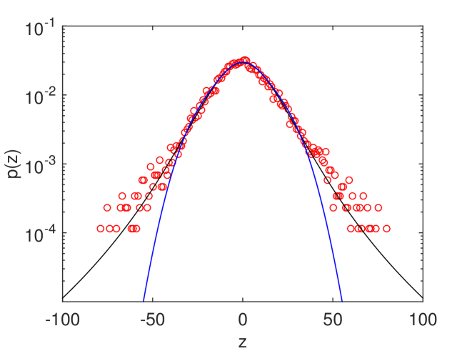
Figure 5: Red circles correspond to histogram data $p(z)$ vs. $z$; solid black line: the $q$-Gaussian function that fits $p(z_{i})$; Blue curve: the best adjustment with the first order q-Gaussian properly normalized

The $q-rel-$value is determined via the temporal self-correlation coefficient

$$C(\tau)=\frac{\sum_{n}Z_{n+\tau}.Z_{n}}{\sum_{n}Z_{n}^{2}}.$$ (4.3)

For a classical BG-process such correlation should decay in exponential fashion, which is not the case for our data. Fig. 2 refers to q-rel. Black circles correspond to the correlation for distinct $\tau$. Black curve: best q-Gaussian-fit to the data and red curve, same for our PDF (1.22).

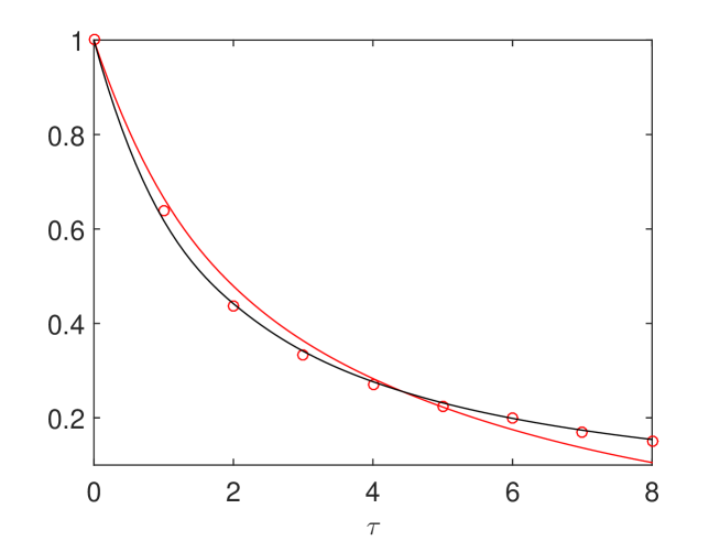
Figure 6: $\ln_{q}$ of the self correlation coefficient $C(\tau)$ vs. time delay $\tau$ (in days). The linear CC is 0.999. Black curve is for a q-Gaussian. Red curve, same for our PDF (1.22).

5 Conclusions

In this effort we have investigated first-order approximations to both 1) Tsallis’ entropy $S_{q}$ and 2) the $S_{q}$-MaxEnt solution (called q-exponential functions $e_{q}$). We were able to show that the functions arising from the MaxEnt treatment 2) are precisely the MaxEnt solutions to the approximate entropy arising from 1). This entails that the approximate entropy is a legitimate new entropic functional.

The present treatment with he new entropy is free of the poles that, for classic quadratic Hamiltonians, appear in Tsallis’ approach, as demonstrated in [Europhysics Letters 104, (2013), 60003], in both the partition function and the mean energy.

We showed that our treatment is compatible with extant date on the ozone layer. The associated q-triplet [25] Tsallis’ $q-$triplet [25] is perhaps the most spectacular empirical quantifier of non-extensivity, i.e., $q\neq 1$. The quantifier was studied in [26] for Tsallis’ entropy, and we see that the present new q-entropy can accommodate the triplet phenomenon.

Finally, we emphasize that the main idea of the current paper is based on the approximation of Eq. (2.1). There is in leading order a quadratic correction term in the variable $U$ if the vicinity of the ordinary Boltzmann factor is considered in the q-statistics approach. This quadradic correction term has been discussed also in [28], where it was also found that the results for small $q-1$ are universal, i.e. applicable to many physical situations in the same way. What is actually new in the current effort is to promote these small $q-1$ effects to yield a new MaxEnt formalism.

Acknowledgment: We thank support from Conicet’s PIP 029/12.

References

- [1] C. Tsallis, J. of Stat. Phys., 52 (1988) 479.
- [2] C. M. Gell-Mann and C. Tsallis, Nonextensive Entropy Interdisciplinary Applications (Oxford University Press, New York, 2004).
- [3] C. Tsallis, Introduction to Nonextensive Statistical Mechanics Approaching a Complex World (Springer, NY, 2009).
- [4] A. Adare et al., Phys. Rev. D 83 (2011) 052004.
- [5] G. Wilk, Z. Wlodarczyk, Physica A 305 (2002) 227.
- [6] R. M. Pickup, R. Cywinski, C. Pappas, B. Farago, and P. Fouquet, Phys. Rev. Lett. 102 (2009) 097202.
- [7] E. Lutz and F. Renzoni, Nature Physics 9 (2013) 615.
- [8] R. G. DeVoe, Phys. Rev. Lett. 102 (2009) 063001.
- [9] Z. Huang, G. Su, A. El Kaabouchi, Q. A. Wang, and J. Chen, J. Stat. Mech. L05001 (2010).
- [10] J. Prehl, C. Essex, and K. H. Hoffman, Entropy 14 (2012) 701.
- [11] B. Liu and J. Goree, Phys. Rev. Lett. 100 (2018) 055003.
- [12] O. Afsar and U. Tirnakli, EPL 101 (2013) 20003.
- [13] U. Tirnakli, C. Tsallis, and C. Beck, Phys. Rev. E 79 (2009) 056209.
- [14] G. Ruiz, T. Bountis, and C. Tsallis, Int. J. Bifurcation Chaos 22 (2012) 1250208.
- [15] C. Beck and S. Miah, Phys. Rev. E 87 (2013) 031002.
- [16] A. A. Budini, Phys. Rev. E 86 (2012) 011109.
- [17] J.-L. Du, J. Stat. Mech. P02006 (2012).
- [18] G. Wilk, Z. Wlodarczyk, Phys. Rev. Lett. 84 (2000) 2770.
- [19] S. Abe, Astrophys. Space Sci. 305, 241 (2006).
- [20] S. Picoli, R. S. Mendes, L. C. Malacarne, and R. P. B. Santos, Braz. J. Phys. 39, 468 (2009).
- [21] A. Plastino and M. C. Rocca Europhysics Letters 104, (2013), 60003.
- [22] G. Y. Shilov: Mathematical Analysis (Pergamon Press, NY, 1965).
- [23] A. Plastino and M. C. Rocca Physica A 436, (2015), 572.
- [24] R.M. Todaro Ed., Stratospheric ozone, NASA’s Goddard Space Flight Center Atmospheric Chemistry and Dynamics Branch. http://www.ccpo.odu.edu/ SEES/ozone/oz_class.htm
- [25] C. Tsallis, Physica A 340 (2004) 1.
- [26] G.L. Ferri, M.F. Reynoso Savio, A. Plastino, Physica A 389 (2010) 1829.
- [27] C. Vignat, A. Plastino. Physica A 388 (2009) 601.
- [28] C. Beck, E.G.D. Cohen, Physica A 322 (2003) 267.
- [29] P. T. Landsberg, Braz. J. Phys. 29 (1999) 46.
- [30] I. S. Gradshteyn and I. M. Rizhik, Table of Integrals Series and Products (Academic Press, NY, 1965, p.285, 3.194,3).
- [31] A. R. Plastino, A Plastino Physics Letters A 177 (1993) 177.
- [32] The procedure we have employed here is usually called “dimensional regularization”.
- [33] A. R. Plastino, A. Plastino, Phys. Lett. A 193 (1994) 140.
- [34] J. J. Atick, E. Witten, Nucl. Phys. B 310 (1988) 291.
- [35] J. Binney and S. Tremaine, Galactic Dynamics (Princeton University Press, Princeton, NJ, 1987).
- [36] E. Verlinde, arXiv:1001.0785 [hep-th]; JHEP 04, 29 (2011).