Distributed Flexible Nonlinear Tensor Factorization

Abstract

Tensor factorization is a powerful tool to analyse multi-way data. Compared with traditional multi-linear methods, nonlinear tensor factorization models are capable of capturing more complex relationships in the data. However, they are computationally expensive and may suffer severe learning bias in case of extreme data sparsity. To overcome these limitations, in this paper we propose a distributed, flexible nonlinear tensor factorization model. Our model can effectively avoid the expensive computations and structural restrictions of the Kronecker-product in existing TGP formulations, allowing an arbitrary subset of tensorial entries to be selected to contribute to the training. At the same time, we derive a tractable and tight variational evidence lower bound (ELBO) that enables highly decoupled, parallel computations and high-quality inference. Based on the new bound, we develop a distributed inference algorithm in the MapReduce framework, which is key-value-free and can fully exploit the memory cache mechanism in fast MapReduce systems such as SPARK. Experimental results fully demonstrate the advantages of our method over several state-of-the-art approaches, in terms of both predictive performance and computational efficiency. Moreover, our approach shows a promising potential in the application of Click-Through-Rate (CTR) prediction for online advertising.

1 Introduction

Tensors, or multidimensional arrays, are generalizations of matrices (from binary interactions) to high-order interactions between multiple entities. For example, we can extract a three-mode tensor (user, advertisement, context) from online advertising data. To analyze tensor data, people usually turn to factorization approaches that use a set of latent factors to represent each entity and model how the latent factors interact with each other to generate tensor elements. Classical tensor factorization models include Tucker  [24] and CANDECOMP/PARAFAC (CP) [8] decompositions, which have been widely used in real-world applications. However, because they all assume a multi-linear interaction between the latent factors, they are unable to capture more complex, nonlinear relationships. Recently,  Xu et al. [25] proposed Infinite Tucker decomposition (InfTucker), which generalizes the Tucker model to infinite feature space using a Tensor-variate Gaussian process (TGP) and thus is powerful to model intricate nonlinear interactions. However, InfTucker and its variants [28, 29] are computationally expensive, because the Kronecker product between the covariances of all the modes requires the TGP to model the entire tensor structure. In addition, they may suffer from the extreme sparsity of real-world tensor data, i.e., when the proportion of the nonzero entries is extremely low. As is often the case, most of the zero elements in real tensors are meaningless: they simply indicate missing or unobserved entries. Incorporating all of them in the training process may affect the factorization quality and lead to biased predictions.

To address these issues, in this paper we propose a distributed, flexible nonlinear tensor factorization model, which has several important advantages. First, it can capture highly nonlinear interactions in the tensor, and is flexible enough to incorporate arbitrary subset of (meaningful) tensorial entries for the training. This is achieved by placing Gaussian process priors over tensor entries, where the input is constructed by concatenating the latent factors from each mode and the intricate relationships are captured by using the kernel function. By using such a construction, the covariance function is then free of the Kronecker-product structure, and as a result users can freely choose any subset of tensor elements for the training process and incorporate prior domain knowledge. For example, one can choose a combination of balanced zero and nonzero elements to overcome the learning bias. Second, the tight variational evidence lower bound (ELBO) we derived using functional derivatives and convex conjugates subsumes optimal variational posteriors, thus evades inefficient, sequential E-M updates and enables highly efficient, parallel computations as well as improved inference quality. Moreover, the new bound allows us to develop a distributed, gradient-based optimization algorithm. Finally, we develop a simple yet very efficient procedure to avoid the data shuffling operation, a major performance bottleneck in the (key-value) sorting procedure in MapReduce. That is, rather than sending out key-value pairs, each mapper simply calculates and sends a global gradient vector without keys. This key-value-free procedure is general and can effectively prevent massive disk IOs and fully exploit the memory cache mechanism in fast MapReduce systems, such as SPARK.

Evaluation using small real-world tensor data have fully demonstrated the superior prediction accuracy of our model in comparison with InfTucker and other state-of-the-art. On large tensors with millions of nonzero elements, our approach is significantly better than, or at least as good as two popular large-scale nonlinear factorization methods based on TGP: one uses hierarchical modeling to perform distributed infinite Tucker decomposition [28]; the other further enhances InfTucker by using Dirichlet process mixture prior over the latent factors and employs an online learning scheme [29]. Our method also outperforms GigaTensor [11], a typical large-scale CP factorization algorithm, by a large margin. In addition, our method achieves faster training speed and enjoys almost linear scalability on the number of computational nodes. We apply our model to CTR prediction for online advertising and achieves a significant, $20\%$ improvement over the popular logistic regression and linear SVM approaches.

2 Background

We first introduce the background knowledge. For convenience, we will use the same notations in [25]. Specifically, we denote a $K$-mode tensor by ${\mathcal{M}}\in\mathbb{R}^{d_{1}\times\ldots\times d_{K}}$, where the $k$-th mode is of dimension $d_{k}$. The tensor entry at location ${\bf i}$ (${\bf i}=(i_{1},\ldots,i_{K})$) is denoted by $m_{\mathbf{i}}$. To introduce Tucker decomposition, we need to generalize matrix-matrix products to tensor-matrix products. Specifically, a tensor $\mathcal{W}\in\mathbb{R}^{r_{1}\times\ldots\times r_{K}}$ can multiply with a matrix ${\bf U}\in\mathbb{R}^{s\times t}$ at mode $k$ when its dimension at mode-$k$ is consistent with the number of columns in ${\bf U}$, i.e., $r_{k}=t$. The product is a new tensor, with size $r_{1}\times\ldots\times r_{k-1}\times s\times r_{k+1}\times\ldots\times r_{K}$. Each element is calculated by $({\mathcal{W}}\times_{k}{\bf U})_{i_{1}\ldots i_{k-1}ji_{k+1}\ldots i_{K}}=\sum_{i_{k}=1}^{r_{k}}w_{i_{1}\ldots i_{K}}u_{ji_{k}}.$

The Tucker decomposition model uses a latent factor matrix ${\bf U}_{k}\in\mathbb{R}^{d_{k}\times r_{k}}$ in each mode $k$ and a core tensor $\mathcal{W}\in\mathbb{R}^{r_{1}\times\ldots\times r_{K}}$ and assumes the whole tensor ${\mathcal{M}}$ is generated by ${\mathcal{M}}={\mathcal{W}}\times_{1}{\bf U}^{(1)}\times_{2}\ldots\times_{K}{\bf U}^{(K)}$. Note that this is a multilinear function of ${\mathcal{W}}$ and $\{{\bf U}_{1},\ldots,{\bf U}_{K}\}$. It can be further simplified by restricting $r_{1}=r_{2}=\ldots=r_{K}$ and the off-diagonal elements of ${\mathcal{W}}$ to be $0$. In this case, the Tucker model becomes CANDECOMP/PARAFAC (CP).

The infinite Tucker decomposition (InfTucker) generalizes the Tucker model to infinite feature space via a tensor-variate Gaussian process (TGP) [25]. Specifically, in a probabilistic framework, we assign a standard normal prior over each element of the core tensor ${\mathcal{W}}$, and then marginalize out ${\mathcal{W}}$ to obtain the probability of the tensor given the latent factors:

$$p({\mathcal{M}}|{\bf U}^{(1)},\ldots,{\bf U}^{(K)})=\mathcal{N}({\rm vec}({\mathcal{M}});{\bf 0},\Sigma^{(1)}\otimes\ldots\otimes\Sigma^{(K)})$$ (1)

where ${\rm vec}{({\mathcal{M}})}$ is the vectorized whole tensor, $\Sigma^{(k)}={\bf U}^{(k)}{{\bf U}^{(k)}}^{\top}$ and $\otimes$ is the Kronecker-product. Next, we apply the kernel trick to model nonlinear interactions between the latent factors: Each row ${\bf u}_{t}^{k}$ of the latent factors ${\bf U}^{(k)}$ is replaced by a nonlinear feature transformation $\phi({\bf u}_{t}^{k})$ and thus an equivalent nonlinear covariance matrix $\Sigma^{(k)}=k({\bf U}^{(k)},{\bf U}^{(k)})$ is used to replace ${\bf U}^{(k)}{{\bf U}^{(k)}}^{\top}$, where $k(\cdot,\cdot)$ is the covariance function. After the nonlinear feature mapping, the original Tucker decomposition is performed in an (unknown) infinite feature space. Further, since the covariance of ${\rm vec}({\mathcal{M}})$ is a function of the latent factors ${\mathcal{U}}=\{{\bf U}^{(1)},\ldots,{\bf U}^{(K)}\}$, Equation (1) actually defines a Gaussian process (GP) on tensors, namely tensor-variate GP (TGP) [25], where the input are based on ${\mathcal{U}}$. Finally, we can use different noisy models $p({\mathcal{Y}}|{\mathcal{M}})$ to sample the observed tensor ${\mathcal{Y}}$. For example, we can use Gaussian models and Probit models for continuous and binary observations, respectively.

3 Model

Despite being able to capture nonlinear interactions, InfTucker may suffer from the extreme sparsity issue in real-world tensor data sets. The reason is that its full covariance is a Kronecker-product between the covariances over all the modes—$\{\Sigma^{(1)},\ldots,\Sigma^{(K)}\}$ (see Equation (1)). Each $\Sigma^{(k)}$ is of size $d_{k}\times d_{k}$ and the full covariance is of size $\prod_{k}d_{k}\times\prod_{k}d_{k}$. Thus TGP is projected onto the entire tensor with respect to the latent factors ${\mathcal{U}}$, including all zero and nonzero elements, rather than a (meaningful) subset of them. However, the real-world tensor data are usually extremely sparse, with a huge number of zero entries and a tiny portion of nonzero entries. On one hand, because most zero entries are meaningless—they are either missing or unobserved, using them can adversely affect the tensor factorization quality and lead to biased predictions; on the other hand, incorporating numerous zero entries into GP models will result in large covariance matrices and high computational costs. Although Zhe et al. [28, 29] proposed to improve the scalability by modeling subtensors instead, the sampled subtensors can still be very sparse. Even worse, because subtensors are typically restricted to a small dimension due to the efficiency considerations, it is often possible to encounter one that does not contain any nonzero entry. This may further incur numerical instabilities in model estimation.

To address these issues, we propose a flexible Gaussian process tensor factorization model. While inheriting the nonlinear modeling power, our model disposes of the Kronecker-product structure in the full covariance and can therefore select an arbitrary subset of tensor entries for training.

Specifically, given a tensor ${\mathcal{M}}\in\mathbb{R}^{d_{1}\times\ldots\times d_{K}}$, for each tensor entry $m_{\bf i}$ (${\bf i}=(i_{1},\ldots,i_{K})$), we construct an input ${\bf x}_{i}$ by concatenating the corresponding latent factors from all the modes: ${\bf x}_{\bf i}=[{\bf u}^{(1)}_{i_{1}},\ldots,{\bf u}^{(K)}_{i_{K}}]$, where ${\bf u}^{(k)}_{i_{k}}$ is the $i_{k}$-th row in the latent factor matrix ${\bf U}^{(k)}$ for mode $k$. We assume that there is an underlying function $f:\mathbb{R}^{\sum_{j=1}^{K}d_{j}}\rightarrow\mathbb{R}$ such that $m_{\bf i}=f({\bf x}_{\bf i})=f([{\bf u}^{(1)}_{i_{1}},\ldots,{\bf u}^{(K)}_{i_{K}}])$. This function is unknown and can be complex and nonlinear. To learn the function, we assign a Gaussian process prior over $f$: for any set of tensor entries $S=\{{\bf i}_{1},\ldots,{\bf i}_{N}\}$, the function values ${\bf f}_{S}=\{f({\bf x}_{{\bf i}_{1}}),\ldots,f({\bf x}_{{\bf i}_{N}})\}$ are distributed according to a multivariate Gaussian distribution with mean ${\bf 0}$ and covariance determined by ${\bf X}_{S}=\{{\bf x}_{{\bf i}_{1}},\ldots,{\bf x}_{{\bf i}_{N}}\}$:

$$p({\bf f}_{S}|{\mathcal{U}})=\mathcal{N}({\bf f}_{S}|{\bf 0},k({\bf X}_{S},{\bf X}_{S}))$$

where $k(\cdot,\cdot)$ is a (nonlinear) covariance function.

Because $k({\bf x}_{\bf i},{\bf x}_{\bf j})=k([{\bf u}^{(1)}_{i_{1}},\ldots,{\bf u}^{(K)}_{i_{K}}],[{\bf u}^{(1)}_{j_{1}},\ldots,{\bf u}^{(K)}_{j_{K}}])$, there is no Kronecker-product structure constraint and so any subset of tensor entries can be selected for training. To prevent the learning process to be biased toward zero, we can use a set of entries with balanced zeros and nonzeros. Furthermore, useful domain knowledge can also be incorporated to select meaningful entries for training. Note, however, that if we still use all the tensor entries and intensionally impose the Kronecker-product structure in the full covariance, our model is reduced to InfTucker. Therefore, from the modeling perspective, the proposed model is more general.

We further assign a standard normal prior over the latent factors ${\mathcal{U}}$. Given the selected tensor entries ${\bf m}=[m_{{\bf i}_{1}},\ldots,m_{{\bf i}_{N}}]$, the observed entries ${\bf y}=[y_{{\bf i}_{1}},\ldots,y_{{\bf i}_{N}}]$ are sampled from a noise model $p({\bf y}|{\bf m})$. In this paper, we deal with both continuous and binary observations. For continuous data, we use the Gaussian model, $p({\bf y}|{\bf m})=\mathcal{N}({\bf y}|{\bf m},\beta^{-1}{\bf I})$ and the joint probability is

$$p({\bf y},{\bf m},{\mathcal{U}}) =\prod\nolimits_{t=1}^{K}\mathcal{N}({\rm vec}({\bf U}^{(t)})|{\bf 0},{\bf I})\mathcal{N}({\bf m}|{\bf 0},k({\bf X}_{S},{\bf X}_{S}))\mathcal{N}({\bf y}|{\bf m},\beta^{-1}{\bf I})$$ (2)

where $S=[{\bf i}_{1},\ldots,{\bf i}_{N}]$. For binary data, we use the Probit model in the following manner. We first introduce augmented variables ${\bf z}=[z_{1},\ldots,z_{N}]$ and then decompose the Probit model into $p(z_{j}|m_{{\bf i}_{j}})=\mathcal{N}(z_{j}|m_{{\bf i}_{j}},1)$ and $p(y_{{\bf i}_{j}}|z_{j})=\mathbbm{1}(y_{{\bf i}_{j}}=0)\mathbbm{1}(z_{j}\leq 0)+\mathbbm{1}(y_{{\bf i}_{j}}=1)\mathbbm{1}(z_{j}>0)$ where $\mathbbm{1}(\cdot)$ is the indicator function. Then the joint probability is

$$p({\bf y},{\bf z},{\bf m},{\mathcal{U}})=\prod\nolimits_{t=1}^{K}\mathcal{N}({\rm vec}({\bf U}^{(t)})|{\bf 0},{\bf I})\mathcal{N}({\bf m}|{\bf 0},k({\bf X}_{S},{\bf X}_{S}))\mathcal{N}({\bf z}|{\bf m},{\bf I})$$

$$\cdot \prod\nolimits_{j}\mathbbm{1}(y_{{\bf i}_{j}}=0)\mathbbm{1}(z_{j}\leq 0)+\mathbbm{1}(y_{{\bf i}_{j}}=1)\mathbbm{1}(z_{j}>0).$$ (3)

4 Distributed Variational Inference

Real-world tensor data often comprise a large number of entries, say, millions of non-zeros and billions of zeros. Even by only using nonzero entries for training, exact inference of the proposed model may still be intractable. This motivates us to develop a distributed variational inference algorithm, presented as follows.

4.1 Tractable Variational Evidence Lower Bound

Since the GP covariance term — $k({\bf X}_{S},{\bf X}_{S})$ (see Equations (2) and (3)) intertwines all the latent factors, exact inference in parallel is difficult. Therefore, we first derive a tractable variational evidence lower bound (ELBO), following the sparse Gaussian process framework by Titsias [23]. The key idea is to introduce a small set of inducing points ${\bf B}=\{{\bf b}_{1},\ldots,{\bf b}_{p}\}$ and latent targets ${\bf v}=\{v_{1},\ldots,v_{p}\}$ ($p\ll N$). Then we augment the original model with a joint multivariate Gaussian distribution of the latent tensor entries ${\bf m}$ and targets ${\bf v}$,

$$p({\bf m},{\bf v}|{\mathcal{U}},{\bf B})=\mathcal{N}(\left[\begin{array}[]{c}{\bf m}\\ {\bf v}\end{array}\right];\left[\begin{array}[]{c}{\bf 0}\\ {\bf 0}\end{array}\right],\left[\begin{array}[]{cc}{\bf K}_{SS}&{\bf K}_{SB}\\ {\bf K}_{BS}&{\bf K}_{BB}\end{array}\right])$$ (10)

where ${\bf K}_{SS}=k({\bf X}_{S},{\bf X}_{S})$, ${\bf K}_{BB}=k({\bf B},{\bf B})$, ${\bf K}_{SB}=k({\bf X}_{S},{\bf B})$ and ${\bf K}_{BS}=k({\bf B},{\bf X}_{S})$. We use Jensen’s inequality and conditional Gaussian distributions to construct the ELBO. Using a very similar derivation to [23], we can obtain a tractable ELBO for our model on continuous data, $\log\big{(}p({\bf y},{\mathcal{U}}|{\bf B})\big{)}\geq L_{1}\big{(}{\mathcal{U}},{\bf B},q({\bf v})\big{)}$ , where

$$L_{1}\big{(}{\mathcal{U}},{\bf B},q({\bf v})\big{)} =\log(p({\mathcal{U}}))+\int q({\bf v})\log\frac{p({\bf v}|{\bf B})}{q({\bf v})}{\rm d}{\bf v}$$

$$+\sum\nolimits_{j}\int q({\bf v})F_{\bf v}(y_{{\bf i}_{j}},\beta){\rm d}{\bf v}.$$ (11)

Here $p({\bf v}|{\bf B})=\mathcal{N}({\bf v}|{\bf 0},K_{BB})$, $q({\bf v})$ is the variational posterior for the latent targets ${\bf v}$ and $F_{\bf v}(\cdot_{j},*)=\int\log\big{(}\mathcal{N}(\cdot_{j}|m_{{\bf i}_{j}},*)\big{)}\mathcal{N}(m_{{\bf i}_{j}}|\mu_{j},\sigma_{j}^{2}){\rm d}m_{{\bf i}_{j}}$, where $\mu_{j}=k({\bf x}_{{\bf i}_{j}},{\bf B}){\bf K}_{BB}^{-1}{\bf v}$ and $\sigma_{j}^{2}=\boldsymbol{\Sigma}(j,j)=k({\bf x}_{{\bf i}_{j}},{\bf x}_{{\bf i}_{j}})-k({\bf x}_{{\bf i}_{j}},{\bf B}){\bf K}_{BB}^{-1}k({\bf B},{\bf x}_{{\bf i}_{j}})$. Note that $L_{1}$ is decomposed into a summation of terms involving individual tensor entries ${\bf i}_{j}(1\leq j\leq N)$. The additive form enables us to distribute the computation across multiple computers.

For binary data, we introduce a variational posterior $q({\bf z})$ and make the mean-field assumption that $q({\bf z})=\prod_{j}q(z_{j})$. Following a similar derivation to the continuous case, we can obtain a tractable ELBO for binary data, $\log\big{(}p({\bf y},{\mathcal{U}}|{\bf B})\big{)}\geq L_{2}\big{(}{\mathcal{U}},{\bf B},q({\bf v}),q({\bf z})\big{)}$, where

$$L_{2}\big{(}{\mathcal{U}},{\bf B},q({\bf v}),q({\bf z})\big{)}=\log(p({\mathcal{U}}))+\int q({\bf v})\log(\frac{p({\bf v}|{\bf B})}{q({\bf v})}){\rm d}{\bf v}$$

$$+\sum\nolimits_{j}q(z_{j})\log(\frac{p(y_{{\bf i}_{j}}|z_{j})}{q(z_{j})})+\sum\nolimits_{j}\int q({\bf v})\int q(z_{j})F_{\bf v}(z_{j},1){\rm d}z_{j}{\rm d}{\bf v}.$$ (12)

One can simply use the standard Expectation-maximization (EM) framework to optimize (11) and (12) for model inference, i.e., the E step updates the variational posteriors $\{q({\bf v}),q({\bf z})\}$ and the M step updates the latent factors ${\mathcal{U}}$, the inducing points ${\bf B}$ and the kernel parameters. However, the sequential E-M updates can not fully exploit the paralleling computing resources. Due to the strong dependencies between the E step and the M step, the sequential E-M updates may take a large number of iterations to converge. Things become worse for binary case: in the E step, the updates of $q({\bf v})$ and $q({\bf z})$ are also dependent on each other, making a parallel inference even less efficient.

4.2 Tight and Parallelizable Variational Evidence Lower Bound

In this section, we further derive tight(er) ELBOs that subsume the optimal variational posteriors for $q({\bf v})$ and $q({\bf z})$. Thereby we can avoid the sequential E-M updates to perform decoupled, highly efficient parallel inference. Moreover, the inference quality is very likely to be improved using tighter bounds. Due to the space limit, we only present key ideas and results here. Detailed discussions are given in Section 1 of the supplementary material.

Tight ELBO for continuous tensors. We take functional derivative of $L_{1}$ with respect to $q({\bf v})$ in (11). By setting the derivative to zero, we obtain the optimal $q({\bf v})$ (which is a Gaussian distribution) and then substitute it into $L_{1}$, manipulating the terms, we achieve the following tighter ELBO.

Theorem 4.1.

For continuous data, we have

$$\log\big{(}p({\bf y},{\mathcal{U}}|{\bf B})\big{)}\geq L_{1}^{*}({\mathcal{U}},{\bf B})=\frac{1}{2}\log|{\bf K}_{BB}|-\frac{1}{2}\log|{\bf K}_{BB}+\beta{\bf A}_{1}|-\frac{1}{2}\beta a_{2}-\frac{1}{2}\beta a_{3}$$

$$+\frac{\beta}{2}{\rm tr}({\bf K}_{BB}^{-1}{\bf A}_{1})-\frac{1}{2}\sum_{k=1}^{K}\|{\bf U}^{(k)}\|^{2}_{F}+\frac{1}{2}\beta^{2}{\bf a}_{4}^{\top}({\bf K}_{BB}+\beta{\bf A}_{1})^{-1}{\bf a}_{4}+\frac{N}{2}\log(\frac{\beta}{2\pi}),$$ (13)

where $\|\cdot\|_{F}$ is Frobenius norm, and

$${\bf A}_{1} =\sum\nolimits_{j}k({\bf B},{\bf x}_{{\bf i}_{j}})k({\bf x}_{{\bf i}_{j}},{\bf B}),\;\;\;\;\;\;\;\;\;\;a_{2}=\sum\nolimits_{j}y_{{\bf i}_{j}}^{2},$$

$$a_{3} =\sum\nolimits_{j}k({\bf x}_{{\bf i}_{j}},{\bf x}_{{\bf i}_{j}}),\;\;\;\;\;\;\;\;\;\;{\bf a}_{4}=\sum\nolimits_{j}k({\bf B},{\bf x}_{{\bf i}_{j}})y_{{\bf i}_{j}}.$$

Tight ELBO for binary tensors. The binary case is more difficult because $q({\bf v})$ and $q({\bf z})$ are coupled together (see (12)). We use the following steps: we first fix $q({\bf z})$ and plug the optimal $q({\bf v})$ in the same way as the continuous case. Then we obtain an intermediate ELBO $\hat{L}_{2}$ that only contains $q({\bf z})$. However, a quadratic term in $\hat{L}_{2}$ , $\frac{1}{2}({\bf K}_{BS}\langle{\bf z}\rangle)^{\top}({\bf K}_{BB}+{\bf A}_{1})^{-1}({\bf K}_{BS}\langle{\bf z}\rangle)$, intertwines all $\{q(z_{j})\}_{j}$ in $\hat{L}_{2}$, making it infeasible to analytically derive or parallelly compute the optimal $\{q(z_{j})\}_{j}$. To overcome this difficulty, we exploit the convex conjugate of the quadratic term to introduce an extra variational parameter $\boldsymbol{\lambda}$ to decouple the dependences between $\{q(z_{j})\}_{j}$. After that, we are able to derive the optimal $\{q(z_{j})\}_{j}$ using functional derivatives and to obtain the following tight ELBO.

Theorem 4.2.

For binary data, we have

$$\log\big{(}p({\bf y},{\mathcal{U}}|{\bf B})\big{)}\geq L_{2}^{*}({\mathcal{U}},{\bf B},\boldsymbol{\lambda})=\frac{1}{2}\log|{\bf K}_{BB}|-\frac{1}{2}\log|{\bf K}_{BB}+{{\bf A}}_{1}|-\frac{1}{2}{a}_{3}$$

$$+\sum_{j}\log\big{(}\Phi((2y_{{\bf i}_{j}}-1)\boldsymbol{\lambda}^{\top}k({\bf B},{\bf x}_{{\bf i}_{j}}))\big{)}-\frac{1}{2}\boldsymbol{\lambda}^{\top}{\bf K}_{BB}\boldsymbol{\lambda}+\frac{1}{2}{\rm tr}({\bf K}_{BB}^{-1}{{\bf A}}_{1})$$

$$-\frac{1}{2}\sum_{k=1}^{K}\|{\bf U}^{(k)}\|^{2}_{F}$$ (14)

where $\Phi(\cdot)$ is the cumulative distribution function of the standard Gaussian.

As we can see, due to the additive forms of the terms in $L_{1}^{*}$ and $L_{2}^{*}$, such as ${\bf A}_{1}$, $a_{2}$, $a_{3}$ and ${\bf a}_{4}$, the computation of the tight ELBOs and their gradients can be efficiently performed in parallel. The derivation of the full gradient is given in Section 2 of the supplementary material.

4.3 Distributed Inference on Tight Bound

4.3.1 Distributed Gradient-based Optimization

Given the tighter ELBOs in (13) and (14), we develop a distributed algorithm to optimize the latent factors ${\mathcal{U}}$, the inducing points ${\bf B}$, the variational parameters $\boldsymbol{\lambda}$ (for binary data) and the kernel parameters. We distribute the computations over multiple computational nodes (Map step) and then collect the results to calculate the ELBO and its gradient (Reduce step). A standard routine, such as gradient descent and L-BFGS, is then used to solve the optimization problem.

For binary data, we further find that $\boldsymbol{\lambda}$ can be updated with a simple fixed point iteration:

$$\boldsymbol{\lambda}^{(t+1)}=({\bf K}_{BB}+{\bf A}_{1})^{-1}({\bf A}_{1}\boldsymbol{\lambda}^{(t)}+{\bf a}_{5})$$ (15)

where ${\bf a}_{5}=\sum_{j}k({\bf B},{\bf x}_{{\bf i}_{j}})(2y_{{\bf i}_{j}}-1)\frac{\mathcal{N}\big{(}k({\bf B},{\bf x}_{{\bf i}_{j}})^{\top}\boldsymbol{\lambda}^{(t)}|0,1\big{)}}{\Phi\big{(}(2y_{{\bf i}_{j}}-1)k({\bf B},{\bf x}_{{\bf i}_{j}})^{\top}\boldsymbol{\lambda}^{(t)}\big{)}}$.

Apparently, the updating can be efficiently performed in parallel (due to the additive structure of ${\bf A}_{1}$ and ${\bf a}_{5}$). Moreover, the convergence is guaranteed by the following lemma. The proof is given in Section 3 of the supplementary material.

Lemma 4.3.

Given ${\mathcal{U}}$ and ${\bf B}$, we have $L_{2}^{*}({\mathcal{U}},{\bf B},\boldsymbol{\lambda}^{t+1})\geq L_{2}^{*}({\mathcal{U}},{\bf B},\boldsymbol{\lambda}^{t})$ and the fixed point iteration (15) always converges.

In our experience, the fixed-point iterations are much more efficient than general search strategies (such as line-search) to identity an appropriate step length along the gradient direction. To use it, before we calculate the gradients with respect to ${\mathcal{U}}$ and ${\bf B}$, we first optimize $\boldsymbol{\lambda}$ using the fixed point iteration (in an inner loop). In the outer control, we then employ gradient descent or L-BFGS to optimize ${\mathcal{U}}$ and ${\bf B}$. This will lead to an even tighter bound for our model: $L_{2}^{**}({\mathcal{U}},{\bf B})=\max\nolimits_{\boldsymbol{\lambda}}L_{2}^{*}({\mathcal{U}},{\bf B},\boldsymbol{\lambda})=\max\nolimits_{q({\bf v}),q({\bf z})}L_{2}({\mathcal{U}},{\bf B},q({\bf v}),q({\bf z}))$. Empirically, this converges must faster than feeding the optimization algorithms with $\partial\lambda$, $\partial{\mathcal{U}}$ and $\partial{\bf B}$ altogether.

4.3.2 Key-Value-Free MapReduce

In this section we present the detailed design of MapReduce procedures to fulfill our distributed inference. Basically, we first allocate a set of tensor entries $S_{t}$ on each Mapper $t$ such that the corresponding components of the ELBO and the gradients are calculated. Then the Reducer aggregates local results from each Mapper to obtain the integrated, global ELBO and gradient.

We first consider the standard (key-value) design. For brevity, we take the gradient computation for the latent factors as an example. For each tensor entry ${\bf i}$ on a Mapper, we calculate the corresponding gradients $\{\partial{\bf u}^{(1)}_{i_{1}},\ldots\partial{\bf u}^{(K)}_{i_{K}}\}$ and then send out the key-value pairs $\{(k,i_{k})\rightarrow\partial{\bf u}^{(k)}_{i_{k}}\}_{k}$, where the key indicates the mode and the index of the latent factors. The Reducer aggregates gradients with the same key to recover the full gradient with respect to each latent factor.

Although the (key-value) MapReduce has been successfully applied in numerous applications, it relies on an expensive data shuffling operation: the Reduce step has to sort the Mappers’ output by the keys before aggregation. Since the sorting is usually performed on disk due to significant data size, intensive disk I/Os and network communications will become serious computational overheads. To overcome this deficiency, we devise a key-value-free Map-Reduce scheme to avoid on-disk data shuffling operations. Specifically, on each Mapper, a complete gradient vector is maintained for all the parameters, including ${\mathcal{U}}$, ${\bf B}$ and the kernel parameters. However, only relevant components of the gradient, as specified by the tensor entries allocated to this Mapper, will be updated. After updates, each Mapper will then send out the full gradient vector, and the Reducer will simply sum them up together to obtain a global gradient vector without having to perform any extra data sorting. Note that a similar procedure can also be used to perform the fixed point iteration for $\boldsymbol{\lambda}$ (in binary tensors).

Efficient MapReduce systems, such as SPARK [27], can fully optimize the non-shuffling Map and Reduce, where most of the data are buffered in memory and disk I/Os are circumvented to the utmost; by contrast, the performance with data shuffling degrades severely [6]. This is verified in our evaluations: on a small tensor of size $100\times 100\times 100$, our key-value-free MapReduce gains $30$ times speed acceleration over the traditional key-value process. Therefore, our algorithm can fully exploit the memory-cache mechanism to achieve fast inference.

4.4 Algorithm Complexity

Suppose we use $N$ tensor entries for training, with $p$ inducing points and $T$ Mapper, the time complexity for each Mapper node is $O(\frac{1}{T}p^{2}N)$. Since $p\ll N$ is a fixed constant ($p=100$ in our experiments), the time complexity is linear in the number of tensor entries. The space complexity for each Mapper node is $O(\sum_{j=1}^{K}m_{j}r_{j}+p^{2}+\frac{N}{T}K)$, in order to store the latent factors, their gradients, the covariance matrix on inducing points, and the indices of the latent factors for each tensor entry. Again, the space complexity is linear in the number of tensor entries. In comparison, InfTucker utilizes the Kronecker-product properties to calculate the gradients and has to perform eigenvalue decomposition of the covariance matrices in each tensor mode. Therefor it has a higher time and space complexity (see  [25] for details) and is not scalable to large dimensions.

5 Related work

Classical tensor factorization models include Tucker [24] and CP [8], based on which many excellent works have been proposed [19, 5, 22, 1, 9, 26, 18, 21, 10, 17]. To deal with big data, several distributed factorization algorithms have been recently developed, such as GigaTensor [11] and DFacTo [4]. Despite the widespread success of these methods, their underlying multilinear factorization structure may limit their capability to capture more complex, nonlinear relationship in real-world applications. Infinite Tucker decomposition [25], and its distributed or online extensions [28, 29] address this issue by modeling tensors or subtensors via a tensor-variate Gaussian process (TGP). However, these methods may suffer from the extreme sparsity in real-world tensor data, because the Kronecker-product structure in the covariance of TGP requires modeling the entire tensor space no matter the elements are meaningful (non-zeros) or not. By contrast, our flexible GP factorization model eliminates the Kronecker-product restriction and can model an arbitrary subset of tensor entries. In theory, all such nonlinear factorization models belong to the random function prior models [14] for exchangeable multidimensional arrays.

Our distributed variational inference algorithm is based on sparse GP [16], an efficient approximation framework to scale up GP models. Sparse GP uses a small set of inducing points to break the dependency between random function values. Recently, Titsias [23] proposed a variational learning framework for sparse GP, based on which Gal et al. [7] derived a tight variational lower bound for distributed inference of GP regression and GPLVM [13]. The derivation of the tight ELBO in our model for continuous tensors is similar to [7]. However, the gradient calculation is substantially different, because the input to our GP factorization model is the concatenation of the latent factors. Many tensor entries may partly share the same latent factors, causing a large amount of key-value pair to be sent during the distributed gradient calculation. This will incur an expensive data shuffling procedure that takes place on disk. To improve the computational efficiency, we develop a non-key-value Map-Reduce to avoid data shuffling and fully exploit the memory-cache mechanism in efficient MapReduce systems. This strategy is also applicable to other Map-Reduce based learning algorithms. In addition to continuous data, we also develop a tight ELBO for binary data on optimal variational posteriors. By introducing $p$ extra variational parameters with convex conjugates ($p$ is the number of inducing points), our inference can be performed efficiently in a distributed manner, which avoids explicit optimization on a large number of variational posteriors for the latent tensor entries and inducing targets. Our method can also be useful for GP classification problem.

6 Experiments

6.1 Evaluation on Small Tensor Data

For evaluation, we first compared our method with various existing tensor factorization methods. To this end, we used four small real datasets where all methods are computationally feasible: (1) Alog, a real-valued tensor of size $200\times 100\times 200$, representing a three-way interaction (user, action, resource) in a file access log. It contains $0.33\%$ nonzero entries.(2) AdClick, a real-valued tensor of size $80\times 100\times 100$, describing (user, publisher, advertisement) clicks for online advertising. It contains $2.39\%$ nonzero entries. (3) Enron, a binary tensor extracted from the Enron email dataset (www.cs.cmu.edu/~./enron/) depicting the three-way relationship (sender, receiver, time). It contains $203\times 203\times 200$ elements, of which $0.01\%$ are nonzero. (4) NellSmall, a binary tensor extracted from the NELL knowledge base (rtw.ml.cmu.edu/rtw/resources), of size $295\times 170\times 94$. It depicts the knowledge predicates (entity, relationship, entity). The data set contains $0.05\%$ nonzero elements.

We compared with CP, nonnegative CP (NN-CP) [19], high order SVD (HOSVD) [12], Tucker, infinite Tucker (InfTucker) Xu et al. [25] and its extension (InfTuckerEx) which uses the Dirichlet process mixture (DPM) prior to model latent clusters and local TGP to perform scalable, online factorization [29]. Note that InfTucker and InfTuckerEx are nonlinear factorization approaches.

For testing, we used the same setting as in [29]. All the methods were evaluated via a 5-fold cross validation. The nonzero entries were randomly split into $5$ folds: $4$ folds were used for training and the remaining non-zero entries and $0.1\%$ zero entries were used for testing so that the number of non-zero entries is comparable to the number of zero entries. By doing this, zero and nonzero entries are treated equally important in testing, and so the evaluation will not be dominated by large portion of zeros. For InfTucker and InfTuckerEx, we carried out extra cross-validations to select the kernel form (e.g., RBF, ARD and Matern kernels) and the kernel parameters. For InfTuckerEx, we randomly sampled subtensors and tuned the learning rate following  [29]. For our model, the number of inducing points was set to $100$, and we used a balanced training set generated as follows: in addition to nonzero entries, we randomly sampled the same number of zero entries and made sure that they would not overlap with the testing zero elements.

Our model used ARD kernel and the kernel parameters were estimated jointly with the latent factors. Thus, the expensive parameter selection procedure was not needed. We implemented our distributed inference algorithm with two optimization frameworks, gradient descent and L-BFGS (denoted by Ours-GD and Ours-LBFGS respectively). For a comprehensive evaluation, we also examined CP on balanced training entries generated in the same way as our model, denoted by CP-2. The mean squared error (MSE) is used to evaluate predictive performance on Alog and Click and area-under-curve (AUC) on Enron and Nell. The averaged results from the $5$-fold cross validation are reported.

Our model achieves a higher prediction accuracy than InfTucker, and a better or comparable accuracy than InfTuckerEx (see Figure 1). A $t$-test shows that our model outperforms InfTucker significantly ($p<0.05$) in almost all situations. Although InfTuckerEx uses the DPM prior to improve factorization, our model still obtains significantly better predictions on Alog and AdClick and comparable or better performance on Enron and NellSmall. This might be attributed to the flexibility of our model in using balanced training entries to prevent the learning bias (toward numerous zeros). Similar improvements can be observed from CP to CP-2. Finally, our model outperforms all the remaining methods, demonstrating the advantage of our nonlinear factorization approach.

6.2 Scalability Analysis

To examine the scalability of the proposed distributed inference algorithm, we used the following large real-world datasets: (1) ACC, A real-valued tensor describing three-way interactions (user, action, resource) in a code repository management system [29]. The tensor is of size $3K\times 150\times 30K$, where $0.009\%$ are nonzero. (2) DBLP: a binary tensor depicting a three-way bibliography relationship (author, conference, keyword) [29]. The tensor was extracted from DBLP database and contains $10K\times 200\times 10K$ elements, where $0.001\%$ are nonzero entries. (3) NELL: a binary tensor representing the knowledge predicates, in the form of (entity, entity, relationship) [28]. The tensor size is $20K\times 12.3K\times 280$ and $0.0001\%$ are nonzero.

The scalability of our distributed inference algorithm was examined with regard to the number of machines on ACC dataset. The number of latent factors was set to 3. We ran our algorithm using the gradient descent. The results are shown in Figure 2(a). The Y-axis shows the reciprocal of the running time multiplied by a constant—which corresponds to the running speed. As we can see, the speed of our algorithm scales up linearly to the number of machines.

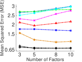
(a) Alog

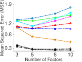
(b) AdClick

(c) Enron

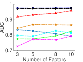
(d) NellSmall

Figure 1: The prediction results on small datasets. The results are averaged over 5 runs.

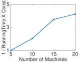
(a) Scalability

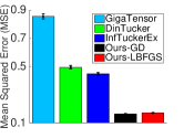
(b) ACC

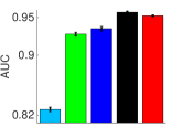
(c) DBLP

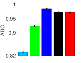
(d) NELL

Figure 2: Prediction accuracy (averaged on $50$ test datasets) on large tensor data and the scalability.

6.3 Evaluation on Large Tensor Data

We then compared our approach with three state-of-the-art large-scale tensor factorization methods: GigaTensor [11], Distributed infinite Tucker decomposition (DinTucker) [28], and InfTuckerEx [29]. Both GigaTensor and DinTucker are developed on Hadoop, while InfTuckerEx uses online inference. Our model was implemented on SPARK. We ran Gigatensor, DinTucker and our approach on a large YARN cluster and InfTuckerEx on a single computer.

We set the number of latent factors to $3$ for ACC and DBLP data set, and $5$ for NELL data set. Following the settings in [29, 28], we randomly chose $80\%$ of nonzero entries for training, and then sampled $50$ test data sets from the remaining entries. For ACC and DBLP, each test data set comprises $200$ nonzero elements and $1,800$ zero elements; for NELL, each test data set contains $200$ nonzero elements and $2,000$ zero elements. The running of GigaTensor was based on the default settings of the software package. For DinTucker and InfTuckerEx, we randomly sampled subtensors for distributed or online inference. The parameters, including the number and size of the subtensors and the learning rate, were selected in the same way as [29]. The kernel form and parameters were chosen by a cross-validation on the training tensor. For our model, we used the same setting as in the small data. We set $50$ Mappers for GigaTensor, DinTucker and our model.

Figure 2(b)-(d) shows the predictive performance of all the methods. We observe that our approach consistently outperforms GigaTensor and DinTucker on all the three datasets; our approach outperforms InfTuckerEx on ACC and DBLP and is slightly worse than InfTuckerEx on NELL. Note again that InfTuckerEx uses DPM prior to enhance the factorization while our model doesn’t; finally, all the nonlinear factorization methods outperform GigaTensor, a distributed CP factorization algorithm by a large margin, confirming the advantages of nonlinear factorizations on large data. In terms of speed, our algorithm is much faster than GigaTensor and DinTucker. For example, on DBLP dataset, the average per-iteration running time were 1.45, 15.4 and 20.5 minutes for our model, GigaTensor and DinTucker, respectively. This is not surprising, because (1) our model uses the data sparsity and can exclude numerous, meaningless zero elements from training; (2) our algorithm is based on SPARK, a more efficient MapReduce system than Hadoop; (3) our algorithm gets rid of data shuffling and can fully exploit the memory-cache mechanism of SPARK.

6.4 Application on Click-Through-Rate Prediction

In this section, we report the results of applying our nonlinear tensor factorization approach on Click-Through-Rate (CTR) prediction for online advertising.

We used the online ads click log from a major Internet company, from which we extracted a four mode tensor (user, advertisement, publisher, page-section). We used the first three days’s log on May 2015, trained our model on one day’s data and used it to predict the click behaviour on the next day. The sizes of the extracted tensors for the three days are $179K\times 81K\times 35\times 355$, $167K\times 78K\times 35\times 354$ and $213K\times 82K\times 37\times 354$ respectively. These tensors are very sparse ($2.7\times 10^{-8}\%$ nonzeros on average). In other words, the observed clicks are very rare. However, we do not want our prediction completely bias toward zero (i.e., non-click); otherwise, ads ranking and recommendation will be infeasible. Thus we sampled non-clicks of the same quantity as the clicks for training and testing. Note that training CTR prediction models with comparable clicks and non-click samples is common in online advertising systems [2]. The number of training and testing entries used for the three days are $(109K,99K)$, $(91K,103K)$ and $(109K,136K)$ respectively.

We compared with popular methods for CTR prediction, including logistic regression and linear SVM, where each tensor entry is represented by a set of binary features according to the indices of each mode in the entry.

The results are reported in Table 1, in terms of AUC. It shows that our model improves logistic regression and linear SVM by a large margin, on average $20.7\%$ and $20.8\%$ respectively. Therefore, although we have not incorporated side features, such as user profiles and advertisement attributes, our tentative experiments have shown a promising potential of our model on CTR prediction task.

Table 1: CTR prediction accuracy on the first three days of May 2015. ”1-2” means using May 1st’s data for training and May 2nd’s data for testing; similar are ”2-3” and ”3-4”.

Method	1-2	2-3	3-4
Logistic regression	0.7360	0.7337	0.7538
Linear SVM	0.7414	0.7332	0.7540
Our model	0.8925	0.8903	0.9054

7 Conclusion

In this paper, we have proposed a new nonlinear and flexible tensor factorization model. By disposing of the Kronecker-product covariance structure, the model can properly exploit the data sparsity and is flexible to incorporate any subset of meaningful tensor entries for training. Moreover, we have derived a tight ELBO for both continuous and binary problems, based on which we further developed an efficient distributed variational inference algorithm in MapReduce framework. In the future, we will consider applying asynchronous inference on the tight ELBO, such as [20], to further improve the scalability of our model.

Supplementary Material

In this extra material, we provide the details about the derivation of the tight variational evidence lower bound of our proposed GP factorization model (Section 1) as well as its gradient calculation (Section 2). Moreover, we give the convergence proof of the fixed point iteration used in our distributed inference algorithm for binary tensor (Section 3).

1 Tight Variational Evidence Lower Bound

The naive variational evidence lower bound (ELBO) derived from the sparse Gaussian process framework (see Section 4.1 of the main paper) is given by

$$L_{1}({\mathcal{U}},{\bf B},q({\bf v})) =\log(p({\mathcal{U}}))+\int q({\bf v})\log\frac{p({\bf v}|{\bf B})}{q({\bf v})}{\rm d}{\bf v}$$

$$+\sum\nolimits_{j}\int q({\bf v})F_{\bf v}(y_{{\bf i}_{j}},\beta){\rm d}{\bf v}$$ (16)

for continuous tensor and

$$L_{2}({\mathcal{U}},{\bf B},q({\bf v}),q({\bf z}))=\log(p({\mathcal{U}}))+\int q({\bf v})\log(\frac{p({\bf v}|{\bf B})}{q({\bf v})}){\rm d}{\bf v}$$

$$+\sum\nolimits_{j}q(z_{j})\log(\frac{p(y_{{\bf i}_{j}}|z_{j})}{q(z_{j})})+\sum\nolimits_{j}\int q({\bf v})\int q(z_{j})F_{\bf v}(z_{j},1){\rm d}z_{j}{\rm d}{\bf v}$$ (17)

for binary tensor, where $F_{\bf v}(\cdot_{j},*)=\int\log\big{(}\mathcal{N}(\cdot_{j}|m_{{\bf i}_{j}},*)\big{)}\mathcal{N}(m_{{\bf i}_{j}}|\mu_{j},\sigma_{j}^{2}){\rm d}m_{{\bf i}_{j}}$ and $p({\bf v}|{\bf B})=\mathcal{N}({\bf v}|{\bf 0},K_{BB})$. Our goal is to further obtain a tight ELBO that subsumes the optimal variational posterior (i.e., $q({\bf v})$ and $q({\bf z})$) so as to prevent the sequential E-M procedure for efficient parallel training and to improve the inference quality.

1.1 Continuous Tensor

First, let us consider the continuous data. Given ${\mathcal{U}}$ and ${\bf B}$, we use functional derivatives [3] to calculate the optimal $q({\bf v})$. The functional derivative of $L_{1}$ with respect to $q({\bf v})$ is given by

$$\frac{\delta L_{1}(q)}{\delta q({\bf v})}=\log\frac{p({\bf v}|{\bf B})}{q({\bf v})}-1+\sum\nolimits_{j}F_{\bf v}(y_{{\bf i}_{j}},\beta).$$

Because $q({\bf v})$ is a probability density function, we use Lagrange multipliers to impose the constraint and obtain the optimal $q({\bf v})$ by solving

$$\frac{\delta\big{(}L_{1}(q)+\lambda(\int q({\bf v}){\rm d}{\bf v}-1)\big{)}}{\delta q({\bf v})} =0,$$

$$\frac{\partial\big{(}L_{1}(q)+\lambda(\int q({\bf v}){\rm d}{\bf v}-1)\big{)}}{\partial\lambda} =0.$$

Though simple algebraic manipulations, we can obtain the optimal $q({\bf v})$ to be the following form

$$q^{*}({\bf v})=\mathcal{N}({\bf v}|\boldsymbol{\mu},\mathbf{\Lambda}),$$

where

$$\boldsymbol{\mu}=\beta{\bf K}_{BB}({\bf K}_{BB}+\beta{\bf K}_{BS}{\bf K}_{SB})^{-1}{\bf K}_{BS}{\bf y},\;\;\;\;\;\mathbf{\Lambda}={\bf K}_{BB}({\bf K}_{BB}+\beta{\bf K}_{BS}{\bf K}_{SB})^{-1}{\bf K}_{BB}.$$

Now substituting $q({\bf v})$ in $L_{1}$ with $\mathcal{N}({\bf v}|\boldsymbol{\mu},\mathbf{\Lambda})$, we obtain the tight ELBO presented in Theorem 4.1 of the main paper:

$$\log\big{(}p({\bf y},{\mathcal{U}}|{\bf B})\big{)}\geq L_{1}^{*}({\mathcal{U}},{\bf B})=\frac{1}{2}\log|{\bf K}_{BB}|-\frac{1}{2}\log|{\bf K}_{BB}+\beta{\bf A}_{1}|-\frac{1}{2}\beta a_{2}-\frac{1}{2}\beta a_{3}$$

$$+\frac{\beta}{2}{\rm tr}({\bf K}_{BB}^{-1}{\bf A}_{1})-\frac{1}{2}\sum_{k=1}^{K}\|{\bf U}^{(k)}\|^{2}_{F}+\frac{1}{2}\beta^{2}{\bf a}_{4}^{\top}({\bf K}_{BB}+\beta{\bf A}_{1})^{-1}{\bf a}_{4}$$

$$+\frac{N}{2}\log(\frac{\beta}{2\pi}),$$ (18)

where $\|\cdot\|_{F}$ is Frobenius norm, and

$${\bf A}_{1} =\sum\nolimits_{j}k({\bf B},{\bf x}_{{\bf i}_{j}})k({\bf x}_{{\bf i}_{j}},{\bf B}),\;\;\;\;\;\;\;\;\;a_{2}=\sum\nolimits_{j}y_{{\bf i}_{j}}^{2},$$

$$a_{3} =\sum\nolimits_{j}k({\bf x}_{{\bf i}_{j}},{\bf x}_{{\bf i}_{j}}),\;\;\;\;\;\;\;\;\;{\bf a}_{4}=\sum\nolimits_{j}k({\bf B},{\bf x}_{{\bf i}_{j}})y_{{\bf i}_{j}}.$$

1.2 Binary Tensor

Next, let us look at the binary data. The case for binary tensors is more complex, because we have the additional variational posterior $q({\bf z})=\prod_{j}q(z_{j})$. Furthermore, $q({\bf v})$ and $q({\bf z})$ are coupled in the original ELBO (see (17)). To eliminate $q({\bf v})$ and $q({\bf z})$, we use the following steps. We first fix $q({\bf z})$, calculate the optimal $q({\bf v})$ and plug it into $L_{2}$ (this is similar to the continuous case) to obtain an intermediate bound,

$$\hat{L}_{2}(q({\bf z}),{\mathcal{U}},{\bf B})=\max\limits_{q({\bf v})}L_{2}(q({\bf v}),q({\bf z}),{\mathcal{U}},{\bf B})$$

$$=\frac{1}{2}\log|{\bf K}_{BB}|-\frac{1}{2}\log|{\bf K}_{BB}+{\bf A}_{1}|-\frac{1}{2}\sum\nolimits_{j}\langle z_{j}^{2}\rangle-\frac{1}{2}a_{3}+\frac{1}{2}{\rm tr}({\bf K}_{BB}^{-1}{\bf A}_{1})$$

$$-\frac{N}{2}\log(2\pi)+\frac{1}{2}({\bf K}_{BS}\langle{\bf z}\rangle)^{\top}({\bf K}_{BB}+{\bf A}_{1})^{-1})({\bf K}_{BS}\langle{\bf z}\rangle)$$

$$+\sum\nolimits_{j}\int q(z_{j})\log(\frac{p(y_{{\bf i}_{j}}|z_{j})}{q(z_{j})}){\rm d}z_{j}-\frac{1}{2}\sum\nolimits_{k=1}^{K}\|{\bf U}^{(k)}\|^{2}_{F}$$ (19)

where $\langle\cdot\rangle$ denotes the expectation under the variational posteriors. Note that $\hat{L}_{2}$ has a similar form to $L_{1}^{*}$ in (18).

Now we consider to calculate the optimal $q({\bf z})$ for $\hat{L}_{2}$. To this end, we calculate the functional derivative of $\hat{L}_{2}$ with respect to each $q(z_{j})$:

$$\frac{\delta\hat{L}_{2}}{\delta q(z_{j})}=\log\frac{p(y_{{\bf i}_{j}}|z_{j})}{q(z_{j})}-1-\frac{1}{2}z_{j}^{2}+c_{jj}\langle z_{j}\rangle z_{j}+\sum_{t\neq j}c_{tj}\langle z_{t}\rangle z_{j}.$$

where $c_{tj}=k({\bf x}_{{\bf i}_{t}},{\bf B})({\bf K}_{BB}+{\bf A}_{1})^{-1}k({\bf B},{\bf x}_{{\bf i}_{j}})$ and $p(y_{{\bf i}_{j}}|z_{j})=\mathbbm{1}\big{(}(2y_{{\bf i}_{j}}-1)z_{j}\geq 0\big{)}$.

Solving $\frac{\delta\hat{L}_{2}}{\delta q(z_{j})}$ being $0$ with Lagrange multipliers, we find that the optimal $q(z_{j})$ is a truncated Gaussian,

$$q^{*}(z_{j})\propto\mathcal{N}(z_{j}|c_{jj}\langle z_{j}\rangle+\sum_{t\neq j}c_{tj}\langle z_{t}\rangle,1)\mathbbm{1}\big{(}(2y_{{\bf i}_{j}}-1)z_{j}\geq 0\big{)}.$$

This expression is unfortunately not analytical. Even if we can explicitly update each $q(z_{j})$, the updating will depend on all the other variational posteriors $\{q(z_{t})\}_{t\neq j}$, making distributed calculation very difficult. This arises from the quadratic term $\frac{1}{2}({\bf K}_{BS}\langle{\bf z}\rangle)^{\top}$
$({\bf K}_{BB}+{\bf A}_{1})^{-1}({\bf K}_{BS}\langle{\bf z}\rangle)$ in (19), which couples all $\{\langle z_{j}\rangle\}_{j}$.

To resolve this issue, we introduce an extra variational parameter $\boldsymbol{\lambda}$ to decouple the dependencies between $\{\langle z_{j}\rangle\}_{j}$ using the following lemma.

Lemma 1.1.

For any symmetric positive definite matrix ${\bf E}$,

$$\boldsymbol{\upeta}^{\top}{\bf E}^{-1}\boldsymbol{\upeta}\geq 2\boldsymbol{\lambda}^{\top}\boldsymbol{\upeta}-\boldsymbol{\lambda}^{\top}{\bf E}\boldsymbol{\lambda}.$$ (20)

The equality is achieved when $\boldsymbol{\lambda}={\bf E}^{-1}\boldsymbol{\upeta}$.

Proof.

Define the function $f(\boldsymbol{\upeta})=\boldsymbol{\upeta}^{\top}{\bf E}^{-1}\boldsymbol{\upeta}$ and it is easy to see that $f(\boldsymbol{\upeta})$ is convex because ${\bf E}^{-1}\succ 0$. Then using the convex conjugate, we have $f(\boldsymbol{\upeta})\geq\boldsymbol{\lambda}^{\top}\boldsymbol{\upeta}-g(\boldsymbol{\lambda})$ and $g(\boldsymbol{\lambda})\geq\boldsymbol{\upeta}^{\top}\boldsymbol{\lambda}-f(\boldsymbol{\upeta})$. Then by maximizing $\boldsymbol{\upeta}^{\top}\boldsymbol{\lambda}-f(\boldsymbol{\upeta})$, we can obtain $g(\boldsymbol{\lambda})=\frac{1}{4}\boldsymbol{\lambda}^{\top}{\bf E}\boldsymbol{\lambda}$. Thus, $f(\boldsymbol{\upeta})\geq\boldsymbol{\lambda}^{\top}\boldsymbol{\upeta}-\frac{1}{4}\boldsymbol{\lambda}^{\top}{\bf E}\boldsymbol{\lambda}$. Since $\boldsymbol{\lambda}$ is a free parameter, we can use $2\boldsymbol{\lambda}$ to replace $\boldsymbol{\lambda}$ and obtain the inequality (20). Further, we can verify that when $\boldsymbol{\lambda}={\bf E}^{-1}\boldsymbol{\upeta}$ the equality is achieved. ∎

We now apply the inequality on the term $\frac{1}{2}({\bf K}_{BS}\langle{\bf z}\rangle)^{\top}({\bf K}_{BB}+{\bf A}_{1})^{-1}{\bf K}_{BS}\langle{\bf z}\rangle$ in (19). Note that the quadratic term regarding all $\{z_{j}\}$ now vanishes, and instead a linear term $\boldsymbol{\lambda}^{\top}{\bf K}_{BS}\langle{\bf z}\rangle$ is introduced so that these annoying dependencies between $\{z_{j}\}_{j}$ are eliminated. We therefore obtain a more friendly intermediate ELBO,

$$\tilde{L}_{2}({\mathcal{U}},{\bf B},q({\bf z}),\boldsymbol{\lambda})=\frac{1}{2}\log|{\bf K}_{BB}|-\frac{1}{2}\log|{\bf K}_{BB}+{\bf A}_{1}|-\frac{1}{2}\sum\nolimits_{j}\langle z_{j}^{2}\rangle-\frac{1}{2}a_{3}$$

$$+\frac{1}{2}{\rm tr}({\bf K}_{BB}^{-1}{{\bf A}}_{1})-\frac{N}{2}\log(2\pi)+\sum\nolimits_{j}\boldsymbol{\lambda}^{\top}k({\bf B},{\bf x}_{{\bf i}_{j}})\langle z_{j}\rangle-\frac{1}{2}\boldsymbol{\lambda}^{\top}({\bf K}_{BB}+{\bf A}_{1})\boldsymbol{\lambda}$$

$$+\sum\nolimits_{j}\int q(z_{j})\log(\frac{p(y_{{\bf i}_{j}}|z_{j})}{q(z_{j})}){\rm d}z_{j}-\frac{1}{2}\sum_{k=1}^{K}\|{\bf U}^{(k)}\|^{2}_{F}.$$ (21)

The functional derivative with respect to $q(z_{j})$ is then given by

$$\frac{\delta\tilde{L}_{2}}{\delta q(z_{j})}=\log\frac{p(y_{{\bf i}_{j}}|z_{j})}{q(z_{j})}-1-\frac{1}{2}z_{j}^{2}+\boldsymbol{\lambda}^{\top}k({\bf B},{\bf x}_{{\bf i}_{j}})z_{j}.$$

Now solving $\frac{\delta\tilde{L}_{2}}{\delta q(z_{j})}=0$, we see that the optimal variational posterior has an analytical form:

$$q^{*}(z_{j})\propto\mathcal{N}(z_{j}|\boldsymbol{\lambda}^{\top}k({\bf B},x_{{\bf i}_{j}}),1)\mathbbm{1}\big{(}(2y_{{\bf i}_{j}}-1)z_{j}\geq 0\big{)}.$$

Plugging each $q^{*}(z_{j})$ into (21), we finally obtain the tight ELBO as presented in Theorem 4.2 of the main paper:

$$\log\big{(}p({\bf y},{\mathcal{U}}|{\bf B})\big{)}\geq L_{2}^{*}({\mathcal{U}},{\bf B},\boldsymbol{\lambda})=\frac{1}{2}\log|{\bf K}_{BB}|-\frac{1}{2}\log|{\bf K}_{BB}+{{\bf A}}_{1}|-\frac{1}{2}{a}_{3}$$

$$+\sum_{j}\log\big{(}\Phi((2y_{{\bf i}_{j}}-1)\boldsymbol{\lambda}^{\top}k({\bf B},{\bf x}_{{\bf i}_{j}}))\big{)}-\frac{1}{2}\boldsymbol{\lambda}^{\top}{\bf K}_{BB}\boldsymbol{\lambda}+\frac{1}{2}{\rm tr}({\bf K}_{BB}^{-1}{{\bf A}}_{1})$$

$$-\frac{1}{2}\sum_{k=1}^{K}\|{\bf U}^{(k)}\|^{2}_{F}.$$ (22)

2 Gradients of the Tight ELBO

In this section, we present how to calculate the gradients of the tight ELBOs in (18) and (22) with respect to the latent factors ${\mathcal{U}}$, the inducing points ${\bf B}$ and the kernel parameters.

Let us first consider the tight ELBO for continuous data. Because ${\mathcal{U}}$, ${\bf B}$ and the kernel parameters are all inside the terms involving the kernel functions, such as ${\bf K}_{BB}$ and ${\bf A}_{1}$, we calculate the gradients with respect to these terms first and then use the chain rule to calculate the gradients with respect to ${\mathcal{U}}$ and ${\bf B}$ and the kernel parameters. Specifically, we consider the derivatives with respect to ${\bf K}_{BB}$, ${\bf A}_{1}$, $a_{3}$ and ${\bf a}_{4}$. Using matrix derivatives and algebras [15], we obtain

$${\rm d}L_{1}^{*} =\frac{1}{2}{\rm tr}\big{(}({\bf K}_{BB}^{-1}-({\bf K}_{BB}+\beta{\bf A}_{1})^{-1}){\rm d}{\bf K}_{BB}\big{)}-\frac{\beta}{2}{\rm tr}\big{(}({\bf K}_{BB}+\beta{\bf A}_{1})^{-1}{\rm d}{\bf A}_{1}\big{)}$$

$$-\frac{\beta}{2}{\rm d}a_{3}-\frac{\beta}{2}{\rm tr}({\bf K}_{BB}^{-1}{\bf A}_{1}{\bf K}_{BB}^{-1}{\rm d}{\bf K}_{BB})+\beta^{2}{\rm tr}({\bf a}_{4}^{\top}({\bf K}_{BB}+\beta{\bf A}_{1})^{-1}{\rm d}{\bf a}_{4})$$

$$+\frac{\beta}{2}{\rm tr}({\bf K}_{BB}^{-1}{\rm d}{\bf A}_{1})-\frac{1}{2}\beta^{2}{\rm tr}\big{(}({\bf K}_{BB}+\beta{\bf A}_{1})^{-1}{\bf a}_{4}{\bf a}_{4}^{\top}({\bf K}_{BB}+\beta{\bf A}_{1})^{-1}{\rm d}{\bf K}_{BB}\big{)}$$

$$-\frac{1}{2}\beta^{3}{\rm tr}\big{(}({\bf K}_{BB}+\beta{\bf A}_{1})^{-1}{\bf a}_{4}{\bf a}_{4}^{\top}({\bf K}_{BB}+\beta{\bf A}_{1})^{-1}{\rm d}{\bf A}_{1}\big{)}.$$ (23)

Next, we calculate the derivatives ${\rm d}{\bf K}_{BB}$, ${\rm d}{\bf A}_{1}$, ${\rm d}a_{3}$ and ${\rm d}{\bf a}_{4}$, which depend on the specific kernel function form used in the model. For example, if we use the linear kernel, ${\rm d}{\bf K}_{BB}=2{\bf B}^{\top}{\rm d}{\bf B}$ and ${\rm d}{\bf A}_{1}=\sum\nolimits_{j=1}^{N}k({\bf B},{\bf x}_{{\bf i}_{j}})({\bf x}_{{\bf i}_{j}}{\rm d}{\bf B}^{\top}+{\rm d}{\bf x}_{{\bf i}_{j}}{\bf B}^{\top})+({\rm d}{\bf B}{\bf x}_{{\bf i}_{j}}^{\top}+{\bf B}{\rm d}{\bf x}_{{\bf i}_{j}}^{\top})k({\bf x}_{{\bf i}_{j}},{\bf B})$ where ${\bf x}_{{\bf i}_{j}}=[{\bf u}^{(1)}_{i_{j1}},\ldots,{\bf u}^{(K)}_{i_{jK}}]$. Note that because ${\bf A}_{1}$, $a_{3}$ and ${\bf a}_{4}$ all have additive structures which involve individual tensor entry ${\bf i}_{j}$ ($1\leq j\leq N$) and the major computation of the derivatives in (23) also involve similar summations, the computation of the final gradients with respect to ${\mathcal{U}}$ and ${\bf B}$ and the kernel parameters can easily be performed in parallel.

The gradient calculation for the tight ELBOs for binary tensors is very similar to the continuous case. Specifically, we obtain

$${\rm d}L_{2}^{*} =\frac{1}{2}{\rm tr}\big{(}{\bf K}_{BB}^{-1}-({\bf K}_{BB}+{\bf A}_{1})^{-1}{\rm d}{\bf K}_{BB}\big{)}-\frac{1}{2}{\rm tr}\big{(}({\bf K}_{BB}+{\bf A}_{1})^{-1}{\rm d}{\bf A}_{1}\big{)}$$

$$-\frac{1}{2}{\rm d}a_{3}-\frac{1}{2}{\rm tr}({\bf K}_{BB}^{-1}{\bf A}_{1}{\bf K}_{BB}^{-1}{\rm d}{\bf K}_{BB})+\frac{1}{2}{\rm tr}({\bf K}_{BB}^{-1}{\rm d}{\bf A}_{1})-\frac{1}{2}{\rm tr}(\boldsymbol{\lambda}\boldsymbol{\lambda}^{\top}{\rm d}{\bf K}_{BB})$$

$$+\sum_{j=1}^{N}(2y_{{\bf i}_{j}}-1)\frac{\mathcal{N}\big{(}\boldsymbol{\lambda}^{\top}k({\bf B},{\bf x}_{{\bf i}_{j}})|0,1\big{)}}{\Phi\big{(}(2y_{{\bf i}_{j}}-1)\boldsymbol{\lambda}^{\top}k({\bf B},{\bf x}_{{\bf i}_{j}})\big{)}}\boldsymbol{\lambda}^{\top}{\rm d}k({\bf B},{\bf x}_{{\bf i}_{j}}).$$ (24)

We can then calculate the derivatives ${\rm d}{\bf K}_{BB}$, ${\rm d}{\bf A}_{1}$, ${\rm d}a_{3}$ and each ${\rm d}k({\bf B},{\bf x}_{{\bf i}_{j}})(1\leq j\leq N)$ and then apply the chain rule to calculate the gradient with respect to ${\mathcal{U}}$, ${\bf B}$ and the kernel parameters.

3 Fixed Point Iteration for $\boldsymbol{\lambda}$

In this section, we give the convergence proof of the fixed point iteration of the variational parameters $\boldsymbol{\lambda}$ in the tight ELBO for binary tensors. While $\boldsymbol{\lambda}$ can be jointly optimized via gradient based approaches with ${\mathcal{U}}$, ${\bf B}$ and the kernel parameters, we empirically find that combining this fixed point iteration can converge much faster. The fixed point iteration is given by

$$\boldsymbol{\lambda}^{(t+1)}=({\bf K}_{BB}+{\bf A}_{1})^{-1}({\bf A}_{1}\boldsymbol{\lambda}^{(t)}+{\bf a}_{5})$$ (25)

where

$${\bf A}_{1} =\sum\nolimits_{j}k({\bf B},{\bf x}_{{\bf i}_{j}})k({\bf x}_{{\bf i}_{j}},{\bf B}),$$

$${\bf a}_{5} =\sum_{j}k({\bf B},{\bf x}_{{\bf i}_{j}})(2y_{{\bf i}_{j}}-1)\frac{\mathcal{N}\big{(}k({\bf B},{\bf x}_{{\bf i}_{j}})^{\top}\boldsymbol{\lambda}^{(t)}|0,1\big{)}}{\Phi\big{(}(2y_{{\bf i}_{j}}-1)k({\bf B},{\bf x}_{{\bf i}_{j}})^{\top}\boldsymbol{\lambda}^{(t)}\big{)}}.$$

We now show that the fixed point iteration not only always converges, but also improves the ELBO in (22) after every update of $\boldsymbol{\lambda}$ (see Lemma 4.3 in the main paper).

Specifically, given ${\mathcal{U}}$ and ${\bf B}$, from Section 1 we have

$$L_{2}^{*}\big{(}\boldsymbol{\lambda}^{(t)}\big{)}=\max\nolimits_{q({\bf z})}\tilde{L}_{2}\big{(}\boldsymbol{\lambda}^{(t)},q({\bf z})\big{)}=\tilde{L}_{2}\big{(}\boldsymbol{\lambda}^{(t)},q_{\boldsymbol{\lambda}^{(t)}}({\bf z})\big{)}$$

where $q_{\boldsymbol{\lambda}^{(t)}}({\bf z})$ is the optimal variational posterior: $q_{\boldsymbol{\lambda}^{(t)}}({\bf z})=\prod_{j}q_{\boldsymbol{\lambda}^{(t)}}(z_{j})$ and $q_{\boldsymbol{\lambda}^{(t)}}(z_{j})\propto\mathcal{N}(z_{j}|k({\bf B},{\bf x}_{{\bf i}_{j}})^{\top}\boldsymbol{\lambda}^{(t)},1)\mathbbm{1}\big{(}(2y_{{\bf i}_{j}}-1)z_{j}\geq 0\big{)}$.

Now let us fix $q_{\boldsymbol{\lambda}^{(t)}}({\bf z})$ and derive the optimal $\boldsymbol{\lambda}$ by solving $\frac{\partial\tilde{L}_{2}}{\partial\boldsymbol{\lambda}}=0$. We then obtain the update of $\boldsymbol{\lambda}$: $\boldsymbol{\lambda}^{(t+1)}=({\bf K}_{BB}+{\bf A}_{1})^{-1}\big{(}\sum_{j}k({\bf B},{\bf x}_{{\bf i}_{j}})\langle z_{j}\rangle\big{)}$ where $\langle z_{j}\rangle$ is the expectation of the optimal variational posterior of $z_{j}$ given $\boldsymbol{\lambda}^{(t)}$, i.e., $q_{\boldsymbol{\lambda}^{(t)}}(z_{j})$. Obviously, we have

$$\tilde{L}_{2}\big{(}\boldsymbol{\lambda}^{(t)},q_{\boldsymbol{\lambda}^{(t)}}({\bf z})\big{)}\leq\tilde{L}_{2}\big{(}\boldsymbol{\lambda}^{(t+1)},q_{\boldsymbol{\lambda}^{(t)}}({\bf z})\big{)}.$$

Further, because $L_{2}^{*}(\boldsymbol{\lambda}^{(t)})=\tilde{L}_{2}\big{(}\boldsymbol{\lambda}^{(t)},q_{\boldsymbol{\lambda}^{(t)}}({\bf z})\big{)}$ and

$$\tilde{L}_{2}\big{(}\boldsymbol{\lambda}^{(t+1)},q_{\boldsymbol{\lambda}^{(t)}}({\bf z})\big{)}\leq\tilde{L}_{2}\big{(}\boldsymbol{\lambda}^{(t+1)},q_{\boldsymbol{\lambda}^{(t+1)}}({\bf z})\big{)}=L_{2}^{*}(\boldsymbol{\lambda}^{(t+1)})$$

we conclude that $L_{2}^{*}(\boldsymbol{\lambda}^{(t)})\leq L_{2}^{*}(\boldsymbol{\lambda}^{(t+1)})$. Now, we plug the fact that $\langle z_{j}\rangle=w_{j}^{(t)}+k({\bf B},{\bf x}_{{\bf i}_{j}})^{\top}\boldsymbol{\lambda}^{(t)}$ given $q_{\boldsymbol{\lambda}^{(t)}}(z_{j})$ into the calculation of $\boldsymbol{\lambda}^{(t+1)}$, merge and arrange the terms. We then obtain the fixed point iteration for $\boldsymbol{\lambda}$ in (25). Finally since $L_{2}^{*}$ is upper bounded by the log model evidence, the fixed point iteration always converges.

References

- Acar et al. [2011] Acar, E., Dunlavy, D. M., Kolda, T. G., & Morup, M. (2011). Scalable tensor factorizations for incomplete data. Chemometrics and Intelligent Laboratory Systems, 106(1), 41–56.
- Agarwal et al. [2014] Agarwal, D., Long, B., Traupman, J., Xin, D., & Zhang, L. (2014). Laser: A scalable response prediction platform for online advertising. In Proceedings of the 7th ACM international conference on Web search and data mining, (pp. 173–182). ACM.
- Bishop [2006] Bishop, C. M. (2006). Pattern recognition and machine learning. springer.
- Choi & Vishwanathan [2014] Choi, J. H. & Vishwanathan, S. (2014). Dfacto: Distributed factorization of tensors. In Advances in Neural Information Processing Systems, (pp. 1296–1304).
- Chu & Ghahramani [2009] Chu, W. & Ghahramani, Z. (2009). Probabilistic models for incomplete multi-dimensional arrays. AISTATS.
- Davidson & Or [2013] Davidson, A. & Or, A. (2013). Optimizing shuffle performance in spark. University of California, Berkeley-Department of Electrical Engineering and Computer Sciences, Tech. Rep.
- Gal et al. [2014] Gal, Y., van der Wilk, M., & Rasmussen, C. (2014). Distributed variational inference in sparse gaussian process regression and latent variable models. In Advances in Neural Information Processing Systems, (pp. 3257–3265).
- Harshman [1970] Harshman, R. A. (1970). Foundations of the PARAFAC procedure: Model and conditions for an”explanatory”multi-mode factor analysis. UCLA Working Papers in Phonetics, 16, 1–84.
- Hoff [2011] Hoff, P. (2011). Hierarchical multilinear models for multiway data. Computational Statistics & Data Analysis, 55, 530–543.
- Hu et al. [2015] Hu, C., Rai, P., & Carin, L. (2015). Zero-truncated poisson tensor factorization for massive binary tensors. In UAI.
- Kang et al. [2012] Kang, U., Papalexakis, E., Harpale, A., & Faloutsos, C. (2012). Gigatensor: scaling tensor analysis up by 100 times-algorithms and discoveries. In Proceedings of the 18th ACM SIGKDD international conference on Knowledge discovery and data mining, (pp. 316–324). ACM.
- Lathauwer et al. [2000] Lathauwer, L. D., Moor, B. D., & Vandewalle, J. (2000). A multilinear singular value decomposition. SIAM J. Matrix Anal. Appl, 21, 1253–1278.
- Lawrence [2004] Lawrence, N. D. (2004). Gaussian process latent variable models for visualisation of high dimensional data. Advances in neural information processing systems, 16(3), 329–336.
- Lloyd et al. [2012] Lloyd, J. R., Orbanz, P., Ghahramani, Z., & Roy, D. M. (2012). Random function priors for exchangeable arrays with applications to graphs and relational data. In Advances in Neural Information Processing Systems 24, (pp. 1007–1015).
- Minka [2000] Minka, T. P. (2000). Old and new matrix algebra useful for statistics. See www. stat. cmu. edu/minka/papers/matrix. html.
- Quiñonero-Candela & Rasmussen [2005] Quiñonero-Candela, J. & Rasmussen, C. E. (2005). A unifying view of sparse approximate gaussian process regression. The Journal of Machine Learning Research, 6, 1939–1959.
- Rai et al. [2015] Rai, P., Hu, C., Harding, M., & Carin, L. (2015). Scalable probabilistic tensor factorization for binary and count data.
- Rai et al. [2014] Rai, P., Wang, Y., Guo, S., Chen, G., Dunson, D., & Carin, L. (2014). Scalable Bayesian low-rank decomposition of incomplete multiway tensors. In Proceedings of the 31th International Conference on Machine Learning (ICML).
- Shashua & Hazan [2005] Shashua, A. & Hazan, T. (2005). Non-negative tensor factorization with applications to statistics and computer vision. In Proceedings of the 22th International Conference on Machine Learning (ICML), (pp. 792–799).
- Smyth et al. [2009] Smyth, P., Welling, M., & Asuncion, A. U. (2009). Asynchronous distributed learning of topic models. In Advances in Neural Information Processing Systems, (pp. 81–88).
- Sun et al. [2015] Sun, W., Lu, J., Liu, H., & Cheng, G. (2015). Provable sparse tensor decomposition. arXiv preprint arXiv:1502.01425.
- Sutskever et al. [2009] Sutskever, I., Tenenbaum, J. B., & Salakhutdinov, R. R. (2009). Modelling relational data using bayesian clustered tensor factorization. In Advances in neural information processing systems, (pp. 1821–1828).
- Titsias [2009] Titsias, M. K. (2009). Variational learning of inducing variables in sparse gaussian processes. In International Conference on Artificial Intelligence and Statistics, (pp. 567–574).
- Tucker [1966] Tucker, L. (1966). Some mathematical notes on three-mode factor analysis. Psychometrika, 31, 279–311.
- Xu et al. [2012] Xu, Z., Yan, F., & Qi, Y. (2012). Infinite Tucker decomposition: Nonparametric Bayesian models for multiway data analysis. In Proceedings of the 29th International Conference on Machine Learning (ICML).
- Yang & Dunson [2013] Yang, Y. & Dunson, D. (2013). Bayesian conditional tensor factorizations for high-dimensional classification. Journal of the Royal Statistical Society B, revision submitted.
- Zaharia et al. [2012] Zaharia, M., Chowdhury, M., Das, T., Dave, A., Ma, J., McCauley, M., Franklin, M. J., Shenker, S., & Stoica, I. (2012). Resilient distributed datasets: A fault-tolerant abstraction for in-memory cluster computing. In Proceedings of the 9th USENIX conference on Networked Systems Design and Implementation, (pp. 2–2). USENIX Association.
- Zhe et al. [2013] Zhe, S., Qi, Y., Park, Y., Molloy, I., & Chari, S. (2013). Dintucker: Scaling up gaussian process models on multidimensional arrays with billions of elements. arXiv preprint arXiv:1311.2663.
- Zhe et al. [2015] Zhe, S., Xu, Z., Chu, X., Qi, Y., & Park, Y. (2015). Scalable nonparametric multiway data analysis. In Proceedings of the Eighteenth International Conference on Artificial Intelligence and Statistics, (pp. 1125–1134).