DASC: Robust Dense Descriptor for Multi-modal and Multi-spectral Correspondence Estimation

Abstract

Establishing dense correspondences between multiple images is a fundamental task in many applications. However, finding a reliable correspondence in multi-modal or multi-spectral images still remains unsolved due to their challenging photometric and geometric variations. In this paper, we propose a novel dense descriptor, called dense adaptive self-correlation (DASC), to estimate multi-modal and multi-spectral dense correspondences. Based on an observation that self-similarity existing within images is robust to imaging modality variations, we define the descriptor with a series of an adaptive self-correlation similarity measure between patches sampled by a randomized receptive field pooling, in which a sampling pattern is obtained using a discriminative learning. The computational redundancy of dense descriptors is dramatically reduced by applying fast edge-aware filtering. Furthermore, in order to address geometric variations including scale and rotation, we propose a geometry-invariant DASC (GI-DASC) descriptor that effectively leverages the DASC through a superpixel-based representation. For a quantitative evaluation of the GI-DASC, we build a novel multi-modal benchmark as varying photometric and geometric conditions. Experimental results demonstrate the outstanding performance of the DASC and GI-DASC in many cases of multi-modal and multi-spectral dense correspondences.

1 Introduction

Recently, many computer vision and computational photography problems have been reformulated to overcome their inherent limitations by leveraging multi-modal and multi-spectral images. Typical examples of other imaging modalities include near-infrared (NIR) image [1, 2] and dark flash image [3]. More broadly, flash and no-flash images [4], blurred images [5, 6], and images taken under different radiometric conditions [7] can also be considered as multi-modal [8].

Establishing dense visual correspondences for multi-modal and multi-spectral images is a key enabler for realizing such tasks. In general, the performance of correspondence algorithms relies primarily on two components: appearance descriptor and optimization scheme. Traditional dense correspondence methods for estimating depth [9] or optical flow [10, 11] fields, in which input images are acquired in a similar imaging condition, have been dramatically advanced in recent studies. To define a matching fidelity term, they typically assume that multiple images share a similar visual pattern, e.g., color, gradient, and structural similarity. However, when it comes to multi-spectral and multi-modal images, such properties do not hold as shown in Fig. 1, and thus conventional descriptors or similarity measures often fail to capture reliable matching evidence.

(a) Image 1

(b) Image 2

(c) DAISY [12]

(d) DASC

Figure 1: Some challenging multi-modal and multi-spectral images such as (from top to bottom) RGB-NIR, flash-noflash images, two images with different exposures, and blur-sharp images. The images in the third and fourth column are the results obtained by warping images in the second column to images in the first column with dense correspondence maps estimated by using DAISY [12] and our DASC descriptor, respectively.

This leads to a poor matching quality as shown in Fig. 2. Furthermore, substantial geometric variations, which often appear in images captured under wide-baseline conditions, make the matching task even more challenging. Although employing a powerful optimization technique could help estimate a reliable solution with a spatial context [13, 14, 15], an optimizer itself cannot address an inherent limitation without suitable matching descriptors [16].

Our method starts from an observation that a local internal layout of self-similarities is less sensitive to photometric distortions, even when an intensity distribution of an anatomical structure is not maintained across different imaging modalities [17]. That is, the local self-similarity (LSS) descriptor would be beneficial to overcoming inherent limitations of existing descriptors in establishing correspondences between multi-modal or multi-spectral images. Several approaches based on the LSS have been presented for multi-modal and multi-spectral image registration [18, 19], but they do not scale well to estimating dense correspondences for multi-modal and multi-spectral images, and their matching performance is still poor.

In this paper, we propose a novel local descriptor, called dense adaptive self-correlation (DASC), designed for establishing dense multi-modal and multi-spectral correspondences. It is defined with a series of patch-wise similarities within a local support window. The similarity is computed with an adaptive self-correlation measure, which encodes an intrinsic structure while providing the robustness against modality variations. To further improve the matching quality and runtime efficiency, we propose a randomized receptive field pooling strategy using sampling patterns that select two patches within the local support window. A linear discriminative learning is employed for obtaining an optimal sampling pattern. The computational redundancy that arises when computing densely sampled descriptors over an entire image is dramatically reduced by applying fast edge-aware filtering [20].

Furthermore, in order to address geometric variation problems such as the scale and rotation, we propose the geometry-invariant DASC (GI-DASC) descriptor that leverages the efficiency and effectiveness of the DASC through a superpixel-based representation. Specifically, we infer an initial geometric field with corresponding scale and rotation of reliable sparse key-points obtained using weighted maximally self-dissimilarity (WMSD), and then propagate the initial geometric field on a superpixel graph. After transforming sampling patterns according to geometric fields on each superpixel, the DASC is efficiently computed with the transformed sampling patterns on each superpixel extended subimage. Compared to conventional geometry-invariant methods for dense correspondence [21, 22], which have been focusing on employing powerful optimization schemes, the GI-DASC provides geometric and photometric robustness on the descriptor itself.

Experimental results show that the DASC outperforms conventional area-based and feature-based approaches on various benchmarks including modality variations; (1) Middlebury stereo benchmark containing illumination and exposure variations [23], (2) multi-modal and multi-spectral dataset including RGB-NIR images [8, 1], different exposure [8, 7], flash-noflash images [7], and blurry images [5, 6], and (3) MPI optical flow benchmark containing specular reflections, motion blur, and defocus blur [10]. We also show that the GI-DASC outperforms existing geometry-invariant methods on a novel multi-modal benchmark.

1.1 Contribution

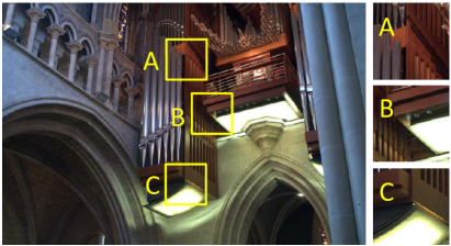
(a) RGB image

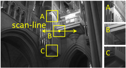
(b) NIR image

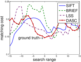
(c) Matching cost in A

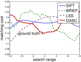
(d) Matching cost in B

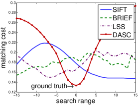
(e) Matching cost in C

Figure 2: Examples of matching cost comparison. Multi-spectral RGB and NIR images have locally non-linear deformation as depicted in A, B, and C. Matching costs computed with different descriptors along A, B, and C’s scan-lines are plotted in (c)-(e). Unlike conventional descriptors, the proposed DASC descriptor yields a reliable global minimum.

The contributions of this paper can be summarized as follows. First, to the best of our knowledge, our approach is the first attempt to design an efficient, dense descriptor for matching multi-modal and multi-spectral images, even under varying geometric conditions. Second, unlike a center-biased dense max pooling, we propose a randomized receptive field pooling with sampling patterns optimized via a discriminative learning, making the descriptor more robust to matching outliers incurred by different imaging modalities. Third, we propose an efficient computational scheme that significantly improves the runtime efficiency of the proposed dense descriptor. Fourth, a geometry-invariant dense descriptor is also proposed, which provides a geometric robustness as a descriptor itself.

This manuscript extends its preliminary version [24]. It newly adds (1) a scale and rotation invariant extension of the DASC, called GI-DASC; (2) a new multi-modal benchmark with a ground truth annotation, captured under varying photometric and geometric conditions; and (3) an intensive comparative study with existing geometry invariant methods using various datasets. The source code of our work (including DASC and GI-DASC) and the new multi-modal benchmark are available at our project webpage [25].

2 Related Work

2.1 Feature Descriptors

As a pioneering work, the scale invariant feature transform (SIFT) was first introduced by Lowe [26] to estimate robust sparse feature correspondence under geometric and photometric variations. Based on the intensity comparison, fast binary descriptors, such as binary robust independent elementary features (BRIEF) [27] and fast retina keypoint (FREAK) [28], have been proposed. Unlike these sparse descriptors, Tola et al. developed a dense descriptor, called DAISY [12], which re-designs conventional sparse descriptors, i.e., SIFT, to efficiently compute densely sampled descriptors over an entire image. Although these conventional gradient-based and intensity comparison-based descriptors show satisfactory performance for small photometric deformation, they cannot properly describe multi-modal and multi-spectral images that often exhibit severe non-linear deformation.

To estimate correspondences in multi-modal and multi-spectral images, some variants of the SIFT have been developed [29], but these gradient-based descriptors have an inherent limitation similar to the SIFT, especially when an image gradient varies across different modality images. Schechtman and Irani introduced the LSS descriptor [17] for the purpose of template matching, and achieved impressive results in object detection and retrieval. Torabi et al. employed the LSS as a multi-spectral similarity metric to register human region of interests (ROIs) [19]. The LSS also has been applied to the registration of multi-spectral remote sensing images [30]. For multi-modal medical image registration, Heinrich et al. proposed a modality independent neighborhood descriptor (MIND) [18] inspired by the LSS. However, none of these approaches scale very well to dense matching tasks for multi-modal and multi-spectral images due to a low discriminative power and a huge complexity.

Recently, several approaches started to employ deep convolutional neural networks (CNNs) [31] for estimating correspondences. For designing explicit, discriminative feature descriptors, intermediate activations from CNN architecture are extracted [32, 33, 34, 35], and they have been shown to be effective for patch-level tasks. However, even though CNN-based descriptors encode a discriminative structure with a deep architecture, they have inherent limitations in multi-modal images, since they use shared convolutional kernels across images which lead to inconsistent responses similar to conventional descriptor [36, 35]. Furthermore, they are unable to provide dense descriptors in the image due to a prohibitively high computational complexity.

2.2 Area-based Similarity Measures

As surveyed in [37], the mutual information (MI), leveraging the entropy of the joint probability distribution function (PDF), has been popularly applied to a registration of multi-modal medical images. However, the MI is sensitive to local radiometric variation since it formulates the intensity variation in a global manner using the joint entropy computed over an entire image. In [38], this issue can be alleviated to some extent by leveraging a locally adaptive weight obtained from SIFT matching, called MI+SIFT in this paper, but its performance is still limited against the multi-modal variation [39]. Although cross-correlation based methods such as an adaptive normalized cross-correlation (ANCC) [40] show satisfactory results for locally linear variations, they show a limitation under severe modality variations. Irani et al. employed the cross-correlation on the Laplacian energy map for measuring multi-sensor image similarity [41], but it also shows a limitation for general image matching tasks. A robust selective normalized cross-correlation (RSNCC) [8] was proposed for the dense alignment between multi-modal images, but its performance is still unsatisfactory due to an inherent limitation of intensity based similarity measure.

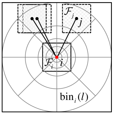
(a) LSS descriptor [17]

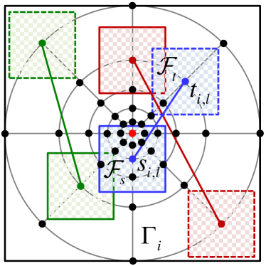
(b) DASC descriptor

Figure 3: Demonstration of the LSS [17] and the DASC descriptor. Within the support window, solid and dotted line box depict source and target patch, respectively. Unlike a center-biased dense max pooling on each $\textrm{bin}_{i}(l)$ in the LSS descriptor, the DASC descriptor incorporates a randomized receptive field pooling using sampling pattern $(s_{i,l},t_{i,l})\in\Lambda_{i}^{\mathrm{dasc}}$ on ${\Gamma_{i}}$, optimized by a discriminative learning.

2.3 Geometry-Invariant Dense Correspondences

Based on the SIFT flow (SF) [13] optimization, many methods have been proposed to alleviate geometric variation problems, including deformable spatial pyramid (DSP) [14], scale-less SIFT flow (SLS) [42], scale-space SIFT flow (SSF) [43], and generalized DSP (GDSP) [22]. However, they have a critical limitation as huge computational complexity derived from dramatically large search space in geometry-invariant dense correspondence. A generalized PatchMatch (GPM) [44] was proposed for efficient matching leveraging a randomized search scheme. The DAISY Filter Flow (DFF) [21], which exploits DAISY descriptor [12] with PatchMatch Filter (PMF) [45], was proposed to provide geometric invariance. However, their weak spatial smoothness often induces mismatched results. The scale invariant descriptor (SID) [46] was proposed to encode geometric robustness on the descriptor itself, but it is not tailored to multi-modal matching. Segmentation-aware approach [47] was proposed to provide geometric robustness for descriptors, e.g., SIFT [26] or SID [46], but it may have a negative effect on the discriminative power of the descriptor.

3 Background

Let us define an image as ${f_{i}}:\mathcal{I}\to{\mathbb{R}}$ for pixel $i$, where $\mathcal{I}\subset{{\mathbb{N}}^{2}}$ is a discrete image domain. Given the image ${f_{i}}$, a dense descriptor ${\mathcal{D}_{i}}:\mathcal{I}\to\mathbb{R}^{L}$ is defined on a local support window $\mathcal{R}_{i}$ centered at pixel $i$ with a feature dimension $L$. Conventionally, descriptors were computed based on the assumption that there is a common underlying visual pattern which is shared by two images. However, as shown in Fig. 2, multi-spectral images such as a pair of RGB-NIR have a nonlinear photometric deformation even within a small window, e.g., gradient reverse and intensity order variation. More seriously, there are outliers including structure divergence caused by shadow or highlight. In these cases, conventional descriptors using an image gradient (SIFT [26]) or an intensity comparison (BRIEF [27]) cannot capture coherent matching evidences, resulting erroneous local minima in estimating dense correspondences.

Unlike these conventional descriptors, the LSS descriptor $\mathcal{D}_{i}^{\textrm{lss}}$ measures a correlation between two patches ${\mathcal{F}_{i}}$ and ${\mathcal{F}_{j}}$ centered at two pixels $i$ and $j$ within a local support window $\mathcal{R}_{i}$ [17]. As shown in Fig. 3(a), it discretizes the correlation surface on a log-polar grid, generates a set of bins, and then stores a maximum correlation value within each bin. Formally, $\mathcal{D}_{i}^{\textrm{lss}}={\bigcup_{l}}d_{i,l}^{\textrm{lss}}$ for $l=1,...,L^{\textrm{lss}}$ is a $L^{\textrm{lss}}\times 1$ feature vector, and $d_{i,l}^{\textrm{lss}}$ can be computed as follows:

$$\begin{array}[]{l}d_{i,l}^{\textrm{lss}}=\mathop{\max}\limits_{j\in\textrm{bin}_{i}(l)}\{\mathcal{C}(i,j)\},\end{array}$$ (1)

where $\textrm{bin}_{i}(l)=\{j|j\in\mathcal{R}_{i},\rho_{r-1}<{|i-j|}\leq\rho_{r},\theta_{a-1}<{\angle(i-j)}\leq\theta_{a}\}$ with a log radius $\rho_{r}$ for $r\in\{1,\cdots,N_{\rho}\}$ and a quantized angle $\theta_{a}$ for $a\in\{1,\cdots,N_{\theta}\}$ with $\rho_{0}=0$ and $\theta_{0}=0$. In that case, $L^{\textrm{lss}}=N_{\rho}\times N_{\theta}$. The correlation surface $\mathcal{C}(i,j)$ is typically computed using a simple similarity metric such as the sum of squared difference (SSD) with a normalization factor $\sigma_{s}$:

$$\mathcal{C}(i,j)=\exp\left({-\textrm{SSD}\left({\mathcal{F}_{i}},{\mathcal{F}_{j}}\right)/\sigma_{s}}\right).$$ (2)

This LSS descriptor has been shown to be robust in cross-domain object detection [17], but it provides unsatisfactory results in densely matching multi-modal images as shown in Fig. 2. It is because the max pooling strategy performed in each $\textrm{bin}_{i}(l)$ loses matching details, leading to a poor discriminative power. Furthermore, the center-biased correlation measure cannot handle severe outliers effectively, which frequently exist in multi-modal and multi-spectral images. In terms of a computational complexity, there exists no efficient computational scheme designed for dense matching descriptor.

4 The DASC Descriptor

4.1 Randomized Receptive Field Pooling

Instead of using a center-biased max pooling of the LSS descriptor in Fig. 3(a), our DASC descriptor incorporates a randomized receptive field pooling with sampling patterns in such a way that a pair of two patches are randomly selected within a local support window. It is motivated by three observations; 1) In multi-spectral and multi-modal images, there frequently exist non-informative regions which are locally degraded, e.g., shadows or outliers. 2) Center-biased pooling is very sensitive to a degradation of a center patch, and cannot deal with a homogeneous or salient center pixel which does not contain self-similarities [17]. 3) From the relationship between Census transform [48] and BRIEF [27] descriptor, it is shown that the randomness enables a descriptor to encode structural information more robustly.

Our approach encodes a similarity between patch-wise receptive fields sampled from log-polar circular point set $\Gamma_{i}$ as shown in Fig. 3(b). It is defined as $\Gamma_{i}=\{j|j\in\mathcal{R}_{i},|{i}-{j}|=\rho_{r},\angle({i}-{j})=\theta_{a}\}$ where the number of points is defined as $N_{c}=N_{\rho}\times N_{\theta}+1$, and has a higher density of points near a center pixel, similar to DAISY descriptor [12]. Given ${N_{c}}$ points in $\Gamma_{i}$, there exist $N_{pc}={\{N_{c}\times(N_{c}-1)\}/2}$ candidate sampling patterns, leading to a dramatically high-dimension descriptor. However, many of the sampling pattern pairs might not be useful in describing a local support window. Therefore, we employ a randomized approach to extract $L^{\mathrm{dasc}}$ sampling patterns from $N_{pc}$ pattern candidates. Our descriptor $\mathcal{D}^{\mathrm{dasc}}_{i}={\bigcup_{l}}d^{\mathrm{dasc}}_{i,l}$ for $l=1,...,L^{\mathrm{dasc}}$ is encoded with a set of patch similarity between two patches based on sampling patterns that are selected from $\Gamma_{i}$:

$$\begin{array}[]{l}d^{\mathrm{dasc}}_{i,l}=\mathcal{C}(s_{i,l},t_{i,l}),\quad s_{i,l},t_{i,l}\in{\Gamma_{i}},\\ \end{array}$$ (3)

where $s_{i,l}$ and $t_{i,l}$ are $l^{th}$ selected sampling patterns at pixel $i$. Note that the sampling patterns are fixed for all pixels in an image. Namely, all pixels share the same set of offset vectors $t_{i,l}-s_{i,l}$ for $l=1,...,L^{\mathrm{dasc}}$, enabling a fast computation of dense descriptors, which will be detailed in Sec. 4.3. Although the DASC descriptor uses only sparse patch-wise pairs in a local support window, many of patches are overlapped when computing patch similarities between the sparse pairs, allowing the descriptor to consider the majority of pixels in the support window and reflect original image attributes effectively.

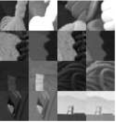
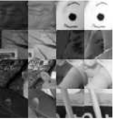
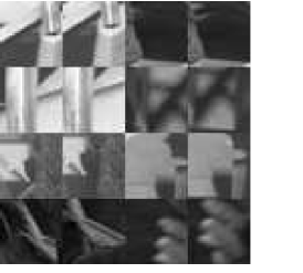
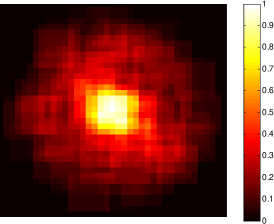
(a) Middlebury [23]

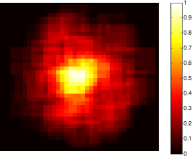
(b) Multi-modal [8]

(c) MPI SINTEL [10]

Figure 4: Visualization of patch-wise receptive fields of the DASC descriptor learned from the training set $\mathcal{P}$ built with the Middlebury benchmark [23], multi-modal benchmark [8], and the MPI SINTEL benchmark [10]. Similar to [49], we stacked all patch-wise receptive fields learned from each training image, and normalized them with the maximal value.

4.1.1 Sampling pattern learning

Finding an optimal sampling pattern is a critical issue in the DASC descriptor. With the assumption that there is no single hand-craft feature that always provides the robustness to all circumstances [49], we employ a discriminative learning to obtain optimal sampling patterns within a local support window. Given candidate sampling patterns $\Lambda_{i}=\{(s_{i,l},t_{i,l})|l=1,...,N_{pc}\}$, our goal is to select the best sampling patterns which derive an important spatial layout.

Our approach exploits support vector machines (SVMs) with a linear kernel [50]. For learning, we build a dataset $\mathcal{P}=\{(\mathcal{R}_{h}^{1},\mathcal{R}_{h}^{2},{y_{h}})|h=1,...,N_{tr}\}$, where $(\mathcal{R}^{1},\mathcal{R}^{2})$ are support window pairs in multi-modal or multi-spectral images, and $N_{tr}$ is the number of training samples. $y$ is a binary label that becomes 1 if two patches are matched, or 0 otherwise. The training data set $\mathcal{P}$ was built with images captured under varying illumination conditions and/or with imaging devices [23, 10, 8]. In experiments, $N_{tr}=10,000$.

First, the feature $\mathbf{r}_{h}={\bigcup_{l}r_{h,l}}$ that describes two support window pairs $\mathcal{R}_{h}^{1}$ and $\mathcal{R}_{h}^{2}$ is defined

$${r_{h,l}}=\exp\left({-{{\left(d_{h,l}^{\mathrm{dasc},1}-d_{h,l}^{\mathrm{dasc},2}\right)}^{2}}/2{\sigma_{r}^{2}}}\right),$$ (4)

where $\sigma_{r}$ is a Gaussian parameter, and $d^{\mathrm{dasc}}_{h,l}$ is the DASC descriptor. The decision function $\mathcal{Q}$ to classify training dataset $\mathcal{P}$ into matching and non-matching can be represented as

$$\mathcal{Q}(\mathbf{r}_{h})=\mathbf{v}^{T}\mathbf{r}_{h}+\mathbf{b},$$ (5)

where the weight $\mathbf{v}={\bigcup_{l}v_{l}}$ indicates an amount of contribution of each candidate sampling pattern, and $\mathbf{b}$ is a bias. Learning $\mathbf{v}$ can be formulated as minimizing

$$\mathbf{E}_{\mathrm{svm}}(\mathbf{v})=\|\mathbf{v}\|^{2}+C_{\mathrm{svm}}\sum\nolimits_{h=1}^{N_{tr}}{l_{\mathrm{hinge}}\left({y_{h}}\cdot\mathcal{Q}(\mathbf{r}_{h})\right)},$$ (6)

where the hinge loss function $l_{\mathrm{hinge}}(x)=\mathrm{max}(0,1-x)$ and $C_{\mathrm{svm}}$ represents a regularization parameter. We use LIBSVM [50] to minimize this objective function. The $|v_{l}|$ encodes the importance of corresponding sampling pattern towards the final decision [51]. Therefore, we rank top $L^{\mathrm{dasc}}$ sampling patterns based on $|v_{l}|$ value, and use them in our descriptor, which is denoted as $\Lambda_{i}^{\mathrm{dasc}}$.

Fig. 4 visualizes learned patch-wise receptive fields of the DASC. It looks similar to the Gaussian weighting, which has been proven to be effective in terms of a structural encoding of descriptor in many literatures [49, 52]. According to training set, it learns optimal receptive fields.

(a) Window 1

(b) Window 2

(c) Gradient orientation

(d) DAISY [12] descriptor

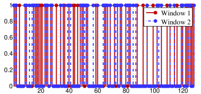
(e) BRIEF [27] descriptor

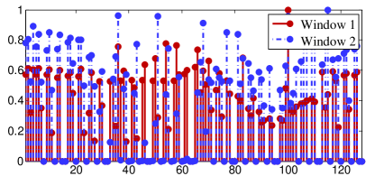
(f) LSS [17] descriptor

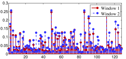
(g) DASC descriptor

Figure 5: Visualization of support window pairs on multi-spectral RGB and NIR images denoted as ‘A’ in Fig. 2 having gradient orientation variations, and descriptors for these window pairs. Conventional descriptors such as DAISY [12], BRIEF [27], and LSS [17] vary across modality variations. Unlike those methods, our DASC descriptor remains unchanged to modality variations.

4.2 Adaptive Self-Correlation Measure

With estimated sampling patterns $(s_{i,l},t_{i,l})$, the DASC descriptor measures a patch similarity using an adaptive self-correlation (ASC) measure in order to robustly encode a local internal layout of self-similarities. For the sake of simplicity, we omit $(i,l)$ in the correlation metric from here on, as it is repeatedly computed for all $(i,l)$. For $(s,t)\in\Lambda^{\mathrm{dasc}}$, the adaptive self-correlation ${\Psi(s,t)}$ between two patches $\mathcal{F}_{s}$ and $\mathcal{F}_{t}$ centered at pixels $s$ and $t$ is computed as follows:

$$\Psi(s,t)=\frac{{\sum\limits_{s^{\prime},t^{\prime}}{{\omega_{s,s^{\prime}}}{\omega_{t,t^{\prime}}}({f_{s^{\prime}}}-{\mathcal{G}_{s}})({f_{t^{\prime}}}-{\mathcal{G}_{t}})}}}{{\sqrt{\sum\limits_{s^{\prime}}{{{\{{\omega_{s,s^{\prime}}}({f_{s^{\prime}}}-{\mathcal{G}_{s}})\}}^{2}}}}\sqrt{\sum\limits_{t^{\prime}}{{{\{{\omega_{t,t^{\prime}}}({f_{t^{\prime}}}-{\mathcal{G}_{t}})\}}^{2}}}}}},$$ (7)

where $s^{\prime}\in\mathcal{F}_{s}$ and $t^{\prime}\in\mathcal{F}_{t}$ and weighted averages on $\mathcal{F}_{s}$ and $\mathcal{F}_{t}$ are defined as ${\mathcal{G}_{s}}=\sum\nolimits_{s^{\prime}}{{\omega_{s,s^{\prime}}}{f_{s^{\prime}}}}$ and ${\mathcal{G}_{t}}=\sum\nolimits_{t^{\prime}}{{\omega_{t,t^{\prime}}}{f_{t^{\prime}}}}$.

The weight ${\omega_{s,s^{\prime}}}$ represents how similar two pixels $s$ and $s^{\prime}$ are, and is normalized, i.e., $\sum\nolimits_{s^{\prime}}{{\omega_{s,s^{\prime}}}}=1$. It can be defined with any kind of edge-aware weights [53, 20, 54]. This weighted sum better handles outliers and local variations in patches compared to other patch-wise similarity metrics. It is worth noting that the adaptive self-correlation used here is conceptually similar to the ANCC [40], but our descriptor employs the correlation metric for measuring self-similarity within a single image which is used for matching two or more images later, while the ANCC is used to directly measure inter-similarity between different images.

Finally, our patch-wise similarity between ${\mathcal{F}_{s}}$ and ${\mathcal{F}_{t}}$ is computed with a truncated exponential function, which has been widely used in the robust estimator [55]:

$$\mathcal{C}(s,t)=\max(\exp(-(1-\left|{\Psi(s,t)}\right|)/\sigma_{c}),\tau_{c}),$$ (8)

where $\sigma_{c}$ is a bandwidth of Gaussian kernel and $\tau_{c}$ is a truncation parameter. Here, a absolute value of ${\Psi(s,t)}$ is used to mitigate the effect of intensity reverses. The correlation $\mathcal{C}(s_{i,l},t_{i,l})$ for $i$ is normalized with an unit norm for all $l$.

Fig. 5 represents examples of visualizing the results of various descriptors. The conventional descriptors show the sensitivity to modality variations, however the DASC shows the robustness against multi-modal variations.

4.3 Efficient Computation for Dense Descriptor

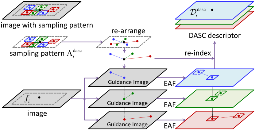
Figure 6: Efficient computation framework of the DASC descriptor. In order to reduce a computational load in computing the adaptive self-correlation, it re-arranges the sampling pattern and employs fast EAF scheme. The DASC descriptor is then computed with re-indexing.

For densely constructing our descriptor on an entire image, we should compute $\mathcal{C}(s_{i,l},t_{i,l})$ for all patch pairs belonging to $(s_{i,l},t_{i,l})\in\Lambda_{i}^{\mathrm{dasc}}$ for each pixel $i$. Thus, a straightforward computation can be extremely time-consuming. In this section, we present an efficient method for computing the DASC descriptor. To compute all weighted sums in (7) for $(s_{i,l},t_{i,l})$ efficiently, we employ a constant-time edge-aware filter (EAF), e.g., the guided filter (GF) [20]. However, the symmetric weight $w_{s,s^{\prime}}w_{t,t^{\prime}}$ varies for each $l$, and thus computing the numerator in (7) is still very time-consuming.

To alleviate these limitations, we simplify (7) by considering only the weight $w_{s,s^{\prime}}$ from the source patch $\mathcal{F}_{s}$ so that a fast computation of (7) using fast edge-aware filter is feasible. It should be noted that such an asymmetric weight approximation also has been used in cost aggregation for stereo matching [56]. We also found that in our descriptor, a performance gap between using the asymmetric weight $w_{s,s^{\prime}}$ and the symmetric weight $w_{s,s^{\prime}}w_{t,t^{\prime}}$ is negligible, which will be shown in Sec. 6.2.5. For efficient description, we also re-arrange the sampling pattern $(s_{i,l},t_{i,l})$ to referenced-biased pairs $(i,j)=(i,i+t_{i,l}-s_{i,l})$. (7) is then approximated as follows:

$$\tilde{\Psi}(i,j)=\frac{{\sum\limits_{i^{\prime},j^{\prime}}{{\omega_{i,i^{\prime}}}({f_{i^{\prime}}}-{\mathcal{G}_{i}})({f_{j^{\prime}}}-{\mathcal{G}_{i,j}})}}}{{\sqrt{\sum\limits_{i^{\prime}}{{{\omega_{i,i^{\prime}}}{({f_{i^{\prime}}}-{\mathcal{G}_{i}})}^{2}}}}\sqrt{\sum\limits_{i^{\prime},j^{\prime}}{{{\omega_{i,i^{\prime}}}{({f_{j^{\prime}}}-{\mathcal{G}_{i,j}})}^{2}}}}}},$$ (9)

where ${\mathcal{G}_{i}}=\sum\nolimits_{i^{\prime}}{{\omega_{i,i^{\prime}}}{f_{i^{\prime}}}}$. Furthermore, ${\mathcal{G}_{i,j}}=\sum\nolimits_{i^{\prime},j^{\prime}}{{\omega_{i,i^{\prime}}}{f_{j^{\prime}}}}$ which means weighted average of $f_{j^{\prime}}\in\mathcal{F}_{j}$ with a guidance image $f_{i^{\prime}}\in\mathcal{F}_{i}$. It is worth noting that the robustness of $\Psi(s,t)$ can be still applied to $\tilde{\Psi}(i,j)$ since their difference is just weight factors.

Algorithm 1: Dense Adaptive Self-Correlation (DASC)
Input : image ${f_{i}}$, candidate sampling patterns $\Lambda_{i}$, training patch pairs dataset $\mathcal{P}$.
Output : the DASC descriptor volume ${\mathcal{D}^{\mathrm{dasc}}_{i}}$.
	$/*$ Offline Procedure $*/$
$\mathbf{1:}$	Compute ${\mathbf{r}_{h}}$ using (4) for possible candidate sampling patterns $\Lambda_{i}$ on training support window pairs $\mathcal{P}$.
$\mathbf{2:}$	Learn a weight ${\mathbf{v}}$ by optimizing (6).
$\mathbf{3:}$	Select the maximal $L^{\mathrm{dasc}}$ sampling patterns $(s_{i,l},t_{i,l})$ in terms of $\left|{v_{l}}\right|$, denoted as $\Lambda_{i}^{\mathrm{dasc}}$.
	$/*$ Online Procedure $*/$
$\mathbf{4:}$	Compute ${\mathcal{G}_{i}}=\sum\nolimits_{i^{\prime}}{{\omega_{i,i^{\prime}}}{f_{i^{\prime}}}}$ for all pixel $i$.
$\mathbf{5:}$	Compute ${\mathcal{G}_{i^{2}}}=\sum\nolimits_{i^{\prime}}{{\omega_{i,i^{\prime}}}f_{i^{\prime}}^{2}}$.
	for $l=1:L^{\mathrm{dasc}}$ do
$\mathbf{6:}$		Re-arrange $(s_{i,l},t_{i,l})\in\Lambda_{i}^{\mathrm{dasc}}$ as $(i,j)=(i,i+t_{i,l}-s_{i,l})$.
$\mathbf{7:}$		Compute ${\mathcal{G}_{i,ij}}=\sum\nolimits_{i^{\prime},j^{\prime}}{{\omega_{i,i^{\prime}}}{f_{i^{\prime}}}{f_{j^{\prime}}}}$.
$\mathbf{8:}$		Compute ${\mathcal{G}_{i,j}}=\sum\nolimits_{i^{\prime},j^{\prime}}{{\omega_{i,i^{\prime}}}{f_{j^{\prime}}}}$.
$\mathbf{9:}$		Compute ${\mathcal{G}_{i,j^{2}}}=\sum\nolimits_{i^{\prime},j^{\prime}}{{\omega_{i,i^{\prime}}}f_{j^{\prime}}^{2}}$.
$\mathbf{10:}$		Estimate ${\tilde{\Psi}(i,i^{\prime})}$ and $\mathcal{C}(i,i^{\prime})$ using (9) and (8).
$\mathbf{11:}$		Compute the DASC descriptor ${\mathcal{D}^{\mathrm{dasc}}_{i}}$ by re-indexing sampling patterns such that ${d^{\mathrm{dasc}}_{i,l}}=\mathcal{C}(s_{i,l},t_{i,l})$.
	end for

We then decompose numerator and denominator in (9) after some arithmetic derivations such that

$$\frac{{{\mathcal{G}_{i,ij}}-{\mathcal{G}_{i}}\cdot{\mathcal{G}_{i,j}}}}{{\sqrt{{\mathcal{G}_{i^{2}}}-{{{\mathcal{G}_{i}^{2}}}}}\cdot\sqrt{{\mathcal{G}_{i,j^{2}}}-{{{\mathcal{G}_{i,j}^{2}}}}}}},$$ (10)

where ${\mathcal{G}_{i^{2}}}=\sum\nolimits_{i^{\prime}}{{\omega_{i,i^{\prime}}}f_{i^{\prime}}^{2}}$, ${\mathcal{G}_{i,ij}}=\sum\nolimits_{i^{\prime},j^{\prime}}{{\omega_{i,i^{\prime}}}{f_{i^{\prime}}}{f_{j^{\prime}}}}$, and ${\mathcal{G}_{i,j^{2}}}=\sum\nolimits_{i^{\prime},j^{\prime}}{{\omega_{i,i^{\prime}}}{f_{j^{\prime}}^{2}}}$. While the ${\mathcal{G}_{i}}$ and ${\mathcal{G}_{i^{2}}}$ can be computed on image domain once, ${\mathcal{G}_{i,ij}}$, ${\mathcal{G}_{i,j}}$, and ${\mathcal{G}_{i,j^{2}}}$ should be computed on each offset. However, the weight $\omega_{i,i^{\prime}}$ is fixed for all offsets, thus it can be shared in all offsets. All these components can be efficiently computed using a constant-time edge-aware filter (EAF) [20]. Finally, the dense descriptor $\mathcal{D}^{\mathrm{dasc}}_{i}$ is computed with re-indexing as ${d^{\mathrm{dasc}}_{i,l}}=\mathcal{C}(s_{i,l},t_{i,l})$ though the robust function in (8). Fig. 6 describes our efficient method for computing the DASC descriptor. Algorithm 1 summarizes the efficient computation of the DASC descriptor.

4.3.1 Comparison of symmetric and asymmetric version of adaptive self-correlation measure

This section analyzes the performance of the DASC descriptor when using the symmetric weight $\omega_{s,s^{\prime}}\omega_{t,t^{\prime}}$ of $\Psi(s,t)$ in (7) and with the asymmetric weight $\omega_{i,{i^{\prime}}}$ of $\tilde{\Psi}(i,j)$ in (9). The symmetric weight case in the DASC can also be computed similar to Sec. 4.3. After re-arranging the sampling pattern as $(i,j)=(i,i+t_{i,l}-s_{i,l})$, the (7) can be then decomposed as similar in (10)

$$\Psi(i,j)=\frac{{{\mathcal{G}_{ij,ij}}-{\mathcal{G}_{ij,i}}-{\mathcal{G}_{ij,j}}+{\mathcal{G}_{i}}\cdot{\mathcal{G}_{j}}}}{{\sqrt{{\mathcal{G}_{i^{2}}}-{{{\mathcal{G}_{i}^{2}}}}}\cdot\sqrt{{\mathcal{G}_{j^{2}}}-{{{\mathcal{G}_{j}^{2}}}}}}},$$ (11)

where ${\mathcal{G}_{ij,ij}}=\sum\nolimits_{i^{\prime}}{{\omega_{i,i^{\prime}}}{\omega_{j,j^{\prime}}}f_{i^{\prime}}^{2}f_{j^{\prime}}^{2}}$, ${\mathcal{G}_{ij,i}}=\sum\nolimits_{i^{\prime},j^{\prime}}{{\omega_{i,i^{\prime}}}{\omega_{j,j^{\prime}}}{f_{i^{\prime}}}}$, and ${\mathcal{G}_{ij,j}}=\sum\nolimits_{i^{\prime},j^{\prime}}{{\omega_{i,i^{\prime}}}{\omega_{j,j^{\prime}}}{f_{j^{\prime}}}}$. The denominator can be easily computed on overall image once. However, compared to the asymmetric measure in (9), $\omega_{i,i^{\prime}}\omega_{j,j^{\prime}}$ in ${\mathcal{G}_{ij,ij}}$, ${\mathcal{G}_{ij,i}}$, and ${\mathcal{G}_{ij,j}}$ varies for each $l$. Furthermore, it should be computed with a range distance using 6-D vector (or 2-D vector), when an input is a color image (or an intensity image). It significantly increases a computational burden needed for employing constant-time EAFs [20, 57]. A performance gap between using the symmetric measure $\Psi(s,t)$ and the asymmetric measure $\tilde{\Psi}(i,j)$ in the DASC descriptor is negligible, which will be shown in Sec. 6.2.5.

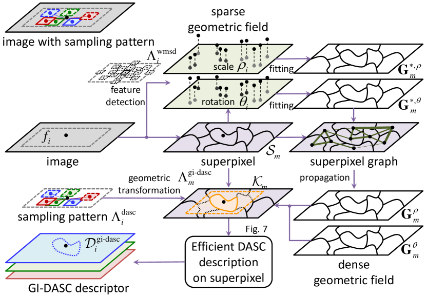
Figure 7: Efficient computation framework of the geometry-invariant DASC (GI-DASC) descriptor. To leverage the efficient computation scheme of the DASC, we employ a superpixel-based description with inferred geometric fields on each superpixel using the WMSD detection.

4.4 Computational Complexity Analysis

The computational complexity of the DASC descriptor on the brute-force implementation becomes $O(INL)$, where $I$, $N$, and $L$ represent an image size, a patch size, and a descriptor dimension, respectively. With our efficient computation model, our approach removes the complexity dependency on the patch size $N$, i.e., $O(IL)$ due to fast constant-time EAF. Furthermore, since there exist repeated offsets, the complexity is further reduced as $O(I\tilde{L})$ for $\tilde{L}<L$.

5 Geometry-Invariant DASC Descriptor

Similar to the DAISY [12], the DASC descriptor is not appropriate to deal with geometric variations. In this section, we propose the geometry-invariant DASC descriptor, called GI-DASC, that addresses severe geometric variations as well as image modality variations. A key idea is to geometrically transform sampling patterns used to measure the patch similarity according to scale and rotation fields when computing the DASC descriptor. To estimate the scale and rotation fields, we first infer initial geometric fields only for sparse points. These initial fields are then fitted and propagated through a superpixel graph. Finally, the GI-DASC descriptor is efficiently computed with geometrically transformed sampling patterns in a manner similar to computing the DASC descriptor, except the fact that the descriptor computation is done for each superpixel independently.

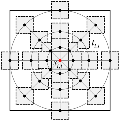
(a) Sampling patterns $\Lambda^{\mathrm{wmsd}}_{i}$

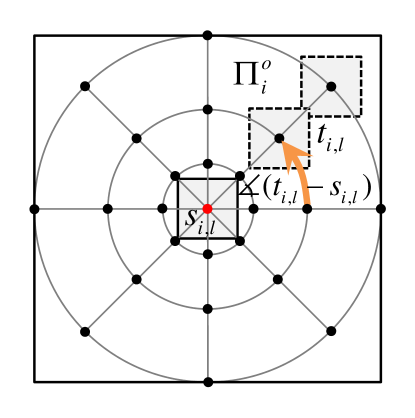
(b) Index set ${\Pi^{o}_{i}}$

Figure 8: Demonstration of sampling patterns $(s_{i,l},t_{t,l})\in\Lambda^{\mathrm{wmsd}}_{i}$ for the WMSD detector and the index set for the $o$ most smallest value ${\Pi^{o}_{i}}$. It enables us to extract reliable feature points $i\in\mathcal{I^{\prime}}$ with corresponding geometric fields (scale $\rho_{i}$ and rotation $\theta_{i}$).

Adopting the superpixel-based geometry field inference has the following three reasons. First, the reliable geometry field can be estimated reliably only at distinctive pixels. Second, the geometric fields tend to vary smoothly, except object boundaries. Third, the transformed sampling patterns should be fixed for each superpixel so that the computational scheme based on the fast EAF [20] can be used for efficiently obtaining the GI-DASC for each superpixel. Fig. 7 represents the overview of the GI-DASC.

5.1 Initial Sparse Geometric Field Inference

Conventional feature detectors, e.g., SIFT [26], are very sensitive to multi-modal and multi-spectral deformation. In order to extract sparse features with distinctive geometric information available, we employ maximal self-dissimilarity (MSD) thanks to its robustness for modality deformation [58]. We propose weighted MSD (WMSD) that improves the performance of the MSD in terms of both complexity and robustness by employing an weighted similarity measure and an efficient computation scheme similar to the DASC.

Similar to $\Gamma_{i}$ used in the DASC, the log-polar circular point set $\Gamma^{\mathrm{wmsd}}_{i}$ is defined for feature detector. The sampling pattern $\Lambda^{\mathrm{wmsd}}_{i}$ is then defined in such a way that the source patch is always located at center pixel and the target patches are located at other neighboring points as shown in Fig. 8(a). In order to consider the scale deformation, we build the Gaussian image pyramid $u^{k}_{i}=f_{i}*\varrho_{k}$ for $k=1,...,N_{k}$, where $\varrho_{k}$ is the $k$-th Gaussian kernel with a sigma $\rho_{k}$ and $N_{k}$ is the number of pyramids. After re-arranging the sampling pattern as $(i,j)=(i,i+t_{i,l}-s_{i,l})$, The self-dissimilarity measure ${\Phi^{k}(i,l)}$ for $l=1,...,L^{\mathrm{wmsd}}(=N^{\mathrm{wmsd}}_{\rho}\times N^{\mathrm{wmsd}}_{\theta})$ is computed using weighted sum of squared difference (SSD) with a guidance image $u^{k}_{i^{\prime}}$ such that

$$\begin{split}{\Phi^{k}(i,l)}&=\sum\nolimits_{i^{\prime},j^{\prime}}{{\omega_{i,{i^{\prime}}}}{{({u^{k}_{i^{\prime}}}-{u^{k}_{j^{\prime}}})}^{2}}}\\ &=\mathcal{U}^{k}_{i^{2}}+\mathcal{U}^{k}_{i,j^{2}}-2\mathcal{U}^{k}_{i,{ij}},\end{split}$$ (12)

where ${\mathcal{U}^{k}_{i^{2}}}=\sum\nolimits_{i^{\prime}}{{\omega_{i,i^{\prime}}}(u^{k}_{i^{\prime}})^{2}}$, ${\mathcal{U}^{k}_{i,j^{2}}}=\sum\nolimits_{i^{\prime},j^{\prime}}{{\omega_{i,i^{\prime}}}(u^{k}_{j^{\prime}})^{2}}$, and ${\mathcal{U}^{k}_{i,ij}}=\sum\nolimits_{i^{\prime},j^{\prime}}{{\omega_{i,i^{\prime}}}u^{k}_{i^{\prime}}u^{k}_{j^{\prime}}}$. Similar to the DASC, (12) can be computed efficiently using constant time EAF [20, 57].

We extract the index set ${\Pi^{o}_{i}}$ for the $o$ most smallest value ${\Psi^{\mathrm{wmsd},k}_{i,l}}$ for all $l$, i.e., $o$ nearest neighbors for center patch in Fig. 8(b). It should be noted that parameter $o$ trades distinctiveness and computational efficiency [58]. We then compute feature response map $\Omega^{k}_{i}$ by estimating the summation of $\Phi^{k}(i,l)$ for ${l\in{\Pi^{o}_{i}}}$ such that

$$\Omega^{k}_{i}=\sum\nolimits_{l\in{\Pi^{o}_{i}}}{\Phi^{k}(i,l)}.$$ (13)

For feature response maps $\mathbf{\Omega}_{i}=\{\Omega^{k}_{i}\}$, the local maxima are obtained by the non maximal suppression, which compares $\Omega^{k}_{i}$ to its $8$ neighbors on the current scale and $18$ neighbors on the $(k+1)^{th}$ and $(k-1)^{th}$ scales. Similar to SIFT [26], a feature point $i\in\mathcal{I^{\prime}}$ is detected only if $\{\Omega^{k}_{i}\}$ has an extreme value compared to all of these neighbors, and its scale $\rho_{i}$ is defined with $\rho_{k}$, where $\mathcal{I^{\prime}}\subset\mathcal{I}$ is a sparse discrete image domain.

A canonical orientation is further associated to $i\in\mathcal{I^{\prime}}$ by constructing a histogram with angles $\measuredangle\left(t_{i,l}-s_{i,l}\right)$ for ${l\in{\Pi^{o}_{i}}}$ weighted by ${\Phi^{k}(i,l)}$ as

$$l_{\mathrm{hist}}(i,\theta)=\sum\nolimits_{l\in{\Pi^{o}_{i}}}{{\Phi^{k}(i,l)}\cdot\delta(\measuredangle\left(t_{i,l}-s_{i,l}\right)-\theta)},$$ (14)

where $\delta$ is the Kronecker delta function. Then, we simply choose the direction corresponding to the highest bin in the histogram, i.e., $\theta_{i}=\mathrm{argmax}_{\theta}l_{\mathrm{hist}}(i,\theta)$. The WMSD detector is summarized in Algorithm 2.

Algorithm 2: Weighted Maximal Self-Dissimilarity (WMSD)
Input : image ${f_{i}}$, feature detection sampling patterns $\Lambda_{i}^{\mathrm{det}}$.
Output : feature points $i\in\mathcal{I^{\prime}}$ with scale $\rho_{i}$, rotation $\theta_{i}$.
	for $k=1:N_{k}$ do
$\mathbf{1:}$		Compute $u^{k}_{i}=f_{i}*\varrho_{k}$ with the Gaussian kernel $\varrho_{k}$.
$\mathbf{2:}$		Compute ${\mathcal{U}^{k}_{i^{2}}}=\sum\nolimits_{i^{\prime}}{{\omega_{i,i^{\prime}}}(u^{k}_{i^{\prime}})^{2}}$ for all pixel $i$.
		for $l=1:L_{\mathrm{wmsd}}$ do
$\mathbf{3:}$			Compute ${\mathcal{U}^{k}_{i,j^{2}}}=\sum\nolimits_{i^{\prime},j^{\prime}}{{\omega_{i,i^{\prime}}}(u^{k}_{j^{\prime}})^{2}}$ for $j=i+t_{i,l}-s_{i,l}$.
$\mathbf{4:}$			Compute ${\mathcal{U}^{k}_{i,ij}}=\sum\nolimits_{i^{\prime},j^{\prime}}{{\omega_{i,i^{\prime}}}u^{k}_{i^{\prime}}u^{k}_{j^{\prime}}}$.
$\mathbf{5:}$			Estimate ${\Phi^{k}(i,l)}=\mathcal{U}^{k}_{i^{2}}+\mathcal{U}^{k}_{i,j^{2}}-2\mathcal{U}^{k}_{i,ij}$.
		end for
$\mathbf{6:}$		Extract the index set ${\Pi^{o}_{i}}$ among ${{\Phi^{k}(i,l)}}$ for all $l$.
$\mathbf{7:}$		Build response map as $\Omega^{k}_{i}=\sum\nolimits_{l\in{\Pi^{o}_{i}}}{{\Phi^{k}(i,l)}}$.
	end for
$\mathbf{8:}$	Detect feature points $i\in\mathcal{I^{\prime}}$ from $\mathbf{\Omega}=\{\Omega^{k}\}$ with scale factor $\rho_{i}$.
$\mathbf{9:}$	Compute the orientation $\theta_{i}$ for $i$ from $l_{\mathrm{hist}}(i,\theta)$.

5.2 Superpixel Graph-Based Propagation

In order to infer dense geometric fields from sparse geometric fields ($\rho_{i}$ and $\theta_{i}$ for $i\in\mathcal{I^{\prime}}$), we decompose the image $f$ as superpixel $\mathcal{S}=\{\mathcal{S}_{m}|\bigcup_{m}\mathcal{S}_{m}=\mathcal{I}\,\mathrm{and}\,\forall m\neq n,\,\mathcal{S}_{m}\bigcap\mathcal{S}_{n}\neq\varnothing,\,m\in 1,...,N_{m}\}$, where $N_{m}$ is the number of superpixels. The geometric field $\mathrm{G}^{*,\rho}_{m}$ and $\mathrm{G}^{*,\theta}_{m}$ are fitted on each superpixel $\mathcal{S}_{m}$ as the average of sparse geometric fields $\rho_{i}$ and $\theta_{i}$ for $i\in\{\mathcal{I^{\prime}}\bigcap\mathcal{S}_{m}\}$. Note that this fitting operation is performed only when $\{\mathcal{I^{\prime}}\bigcap\mathcal{S}_{m}\}$ exists, i.e., the superpixel includes sparse feature points (at least, 1). Finally, the $\mathbf{G}^{*,\rho}={\bigcup_{m}}{\mathrm{G}^{*,\rho}_{m}}\in\mathbb{R}^{N_{m}}$ and $\mathbf{G}^{*,\theta}={\bigcup_{m}}{\mathrm{G}^{*,\theta}_{m}}$ are constructed for all superpixels.

Similar to [59], our approach then formulates an inference of dense geometric fields $\mathbf{G}^{\rho}$ and $\mathbf{G}^{\theta}$ as a constrained optimization problem where surface-fitted sparse geometric fields $\mathbf{G}^{*,\rho}$ and $\mathbf{G}^{*,\theta}$ are interpreted as soft constraints. For the sake of simplicity, we omit ${\rho}$ and ${\theta}$ since they can be computed using the same method. The energy function of our superpixel-based propagation is defined as follows:

$$\sum\limits_{m}\left\{{p^{\mathrm{sp}}_{m}}{{{({\mathrm{G}_{m}}-\mathrm{G}_{m}^{*})}^{2}}}+\mu\sum\limits_{n\in{\mathcal{N}_{m}}}{{\omega^{\mathrm{sp}}_{mn}}({\mathrm{G}_{m}}-{\mathrm{G}_{n}})^{2}}\right\},$$ (15)

where $\mu$ is a regularization parameter. Here, the first term encodes the dissimilarity between final geometric fields ${\mathrm{G}_{m}}$ and initial sparse geometric fields ${\mathrm{G}^{*}_{m}}$. ${p^{\mathrm{sp}}_{m}}$ is an index function, which is 1 for valid (constraint) superpixel, and 0 otherwise. The second term imposes the constraint that two adjacent superpixels ${m}$ and ${n\in{\mathcal{N}_{m}}}$ may have similar geometric fields according to surperpixel feature affinity ${\omega^{\mathrm{sp}}_{mn}}$, which will be described in the following section.

(a) Image 1

(b) Image 2

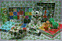
(c) Superpixel 1

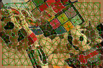
(d) Superpixel 2

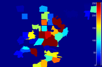
(e) $\mathbf{G}^{*,\rho}_{1}$

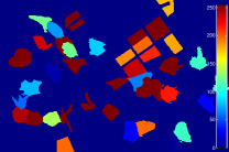
(f) $\mathbf{G}^{*,\rho}_{2}$

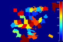
(g) $\mathbf{G}^{*,\theta}_{1}$

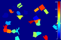
(h) $\mathbf{G}^{*,\theta}_{2}$

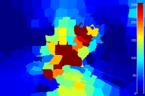
(i) $\mathbf{G}^{\rho}_{1}$

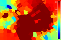
(j) $\mathbf{G}^{\rho}_{2}$

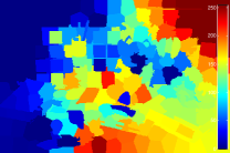
(k) $\mathbf{G}^{\theta}_{1}$

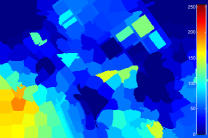
(l) $\mathbf{G}^{\theta}_{2}$

Figure 9: Examples of a superpixel graph-based propagation. With each superpixel graph in (c), (d) for input images in (a), (b), sparse geometric fields (scale $\mathbf{G}^{*,\rho}$, rotation $\mathbf{G}^{*,\theta}$) in (e)-(h) are propagated into dense geometric fields (scale $\mathbf{G}^{\rho}$, rotation $\mathbf{G}^{\theta}$) in (i)-(l).

5.2.1 Superpixel feature affinity

Our approach employs a superpixel feature composed of an appearance and a spatial feature. First, appearance feature $\upsilon_{m}^{c}$ is defined as the average and standard deviation for intensities of pixels within superpixels. In experiments, we used RGB, Lab, and YCbCr space for a color image, thus $\upsilon_{m}^{c}\in\mathbb{R}^{18}$. For an NIR image, appearance feature is defined on 1-channel intensity domain such that $\upsilon_{m}^{c}\in\mathbb{R}^{2}$. Note that directly constructing an affinity matrix with intensity values may lead to inaccurate results due to intensity variations. However, the effect on such variations can be greatly reduced, since the appearance feature is defined as an aggregated form within a superpixel and the affinity value is measured within the same image domain. Second, spatial feature $\upsilon_{m}^{p}\in\mathbb{R}^{2}$ is defined as a spatial centroid coordinate within superpixels. Based on these superpixel features, a superpixel feature affinity ${\omega^{\mathrm{sp}}_{mn}}$ between two adjacent superpixel $m$ and $n\in\mathcal{N}_{m}$ is computed as

$${\omega^{\mathrm{sp}}_{mn}}=\exp(-{\left\|{\upsilon_{m}^{c}-\upsilon_{n}^{c}}\right\|^{2}}/{\lambda_{c}}-{\left\|{\upsilon_{m}^{p}-\upsilon_{n}^{p}}\right\|^{2}}/{\lambda_{p}}),$$ (16)

where ${\lambda_{c}}$ and ${\lambda_{p}}$ denote coefficients for controlling the spatial coherence of neighboring superpixels.

5.2.2 Solver

The minimum of the energy function (15) can be obtained with the following linear system

$$(\mathbf{P}+\mu\mathbf{U}-\mu\mathbf{W})\mathbf{G}=\mathbf{P}\mathbf{G}^{\mathbf{*}},$$ (17)

where $\mathbf{P}_{mm}=\mathrm{diag}[p^{\mathrm{sp}}_{1},...,p^{\mathrm{sp}}_{N_{m}}]$, $\mathbf{U}_{mm}=\mathrm{diag}[u^{\mathrm{sp}}_{1},...,u^{\mathrm{sp}}_{N_{m}}]$ where $u^{\mathrm{sp}}_{m}=\sum\nolimits_{n\in{\mathcal{N}_{m}}}{\omega^{\mathrm{sp}}_{mn}}$, and ${\mathbf{W}}=[\omega^{\mathrm{sp}}_{mn}]_{m,n=1,...,N_{m}}$.

This linear system with a Laplacian matrix can be easily solved with conventional linear solvers [60]. Fig. 9 shows examples of our superpixel graph-based propagation.

5.3 Efficient Dense Descriptor on Superpixels

The sampling patterns are transformed with corresponding geometric fields $\mathbf{G}^{\rho}$ and $\mathbf{G}^{\theta}$ as shown in Fig. 10. Specifically, for the $m$-th superpixel $\mathcal{S}_{m}$, the sampling pattern $(s_{m,l},t_{m,l})\in\Lambda^{\mathrm{gi-dasc}}_{m}$ is transformed from $(s_{l},t_{l})\in\Lambda^{\mathrm{dasc}}$ with a scale factor $\mathrm{G}^{\rho}_{m}$ and a rotation factor $\mathrm{G}^{\theta}_{m}$,

$$s_{m,l}=\mathbf{S}_{m}\mathbf{R}_{m}s_{l},$$ (18)

where the scale matrix $\mathbf{S}_{m}=\mathrm{diag}[\mathrm{G}^{\rho}_{m}]$ and the rotation matrix $\mathbf{R}_{m}$ is defined with rotation $\mathrm{G}^{\theta}_{m}$. In a similar way, $t_{m,l}$ is also estimated from $t_{l}$. Finally, $\Lambda^{\mathrm{gi-dasc}}_{m}$ is estimated. Furthermore, the patch size $N$ is enlarged as $N\mathrm{G}^{\rho}_{m}$.

Algorithm 3: Geometric-Invariant DASC (GI-DASC)
Input : image ${f_{i}}$, feature detection sampling patterns $\Lambda_{i}^{\mathrm{det}}$, $L^{\mathrm{dasc}}$ sampling patterns $(s_{i,l},t_{i,l})\in\Lambda_{i}^{\mathrm{dasc}}$.
Output : the GI-DASC descriptor volume ${\mathcal{D}^{\mathrm{gi-dasc}}_{i}}$.
$\mathbf{1:}$	Extract feature points $i\in\mathcal{I^{\prime}}$ with scale $\rho_{i}$ and rotation $\theta_{i}$ using Algorithm 2.
$\mathbf{2:}$	Decompose the image ${f_{i}}$ into superpixels $\mathcal{S}$.
$\mathbf{3:}$	Compute a surface fitting for geometric field $\mathbf{G}^{*,\rho}_{m}$ and $\mathbf{G}^{*,\theta}_{m}$ on superpixels $\mathcal{S}_{m}$.
$\mathbf{4:}$	Compute a Laplacian matrix ${\mathbf{P}+\mu\mathbf{U}-\mu\mathbf{}W}$ with confidences ${p^{\mathrm{sp}}_{m}}$ and weights ${\omega^{\mathrm{sp}}_{mn}}$.
$\mathbf{5:}$	Compute dense geometric fields $\mathbf{G}^{\rho}_{m}$ and $\mathbf{G}^{\theta}_{m}$.
	for $m=1:N_{m}$ do
$\mathbf{6:}$		Transform the sampling pattern $\Lambda_{i}^{\mathrm{dasc}}$ into $\Lambda_{m}^{\mathrm{gi-dasc}}$.
$\mathbf{7:}$		Compute the GI-DASC descriptor ${d^{\mathrm{gi-dasc}}_{i,l}}=\mathcal{C}(s_{i,l},t_{i,l})$ for $i\in\mathcal{S}_{m}$ and $(s_{m,l},t_{m,l})\in\Lambda^{\mathrm{gi-dasc}}_{m}$ using Algorithm 1.
	end for

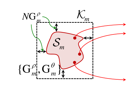
(a) Superpixel extended subimage

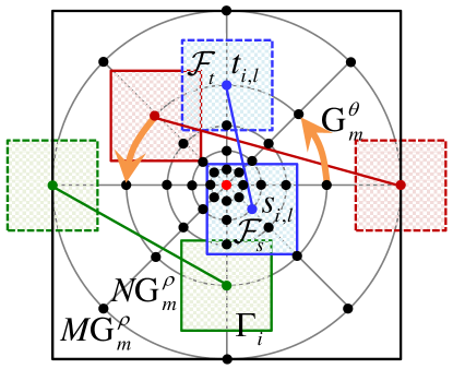
(b) Sampling pattern $\Lambda_{m}^{\mathrm{gi-dasc}}$

Figure 10: Sampling pattern transformation in the GI-DASC descriptor. The sampling patterns $(s_{i,l},t_{i,l})\in\Lambda_{i}^{\mathrm{dasc}}$ is transformed as $(s_{m,l},t_{m,l})\in\Lambda_{m}^{\mathrm{gi-dasc}}$ with $\mathrm{G}^{\rho}_{m}$ and $\mathrm{G}^{\theta}_{m}$ on superpixel $\mathcal{S}_{m}$, which is applied equally for all $i\in\mathcal{S}_{m}$. It provides the geometric robustness on each superpixel.

The $m$-th superpixel extended subimage $\mathcal{K}_{m}$ in Fig. 10(a) is filtered by a Gaussian filtering with the sigma $\{(\mathrm{G}^{\rho}_{m})^{2}-0.25\}^{-1/2}$ similar to scale-space theory used in the SIFT [26]. Then, our GI-DASC descriptor $\mathcal{D}^{\mathrm{gi-dasc}}_{i}={\bigcup_{l}}d^{\mathrm{gi-dasc}}_{i,l}$ for $l=1,...,L^{\mathrm{gi-dasc}}$ ($=L^{\mathrm{dasc}}$) is encoded with a set of patch similarity between two patches from a transformed sampling pattern $\Lambda^{\mathrm{gi-dasc}}_{m}$ on each superpixel $\mathcal{S}_{m}$ such that

$$\begin{array}[]{l}d^{\mathrm{gi-dasc}}_{i,l}=\mathcal{C}(s_{i,l},t_{i,l}),\quad(s_{i,l},t_{i,l})\in\Lambda^{\mathrm{gi-dasc}}_{m},\\ \end{array}$$ (19)

for $i\in{\mathcal{S}_{m}}$. Finally, the dense GI-DASC descriptor is efficiently computed for all the superpixels $\mathcal{S}_{m}\in\mathcal{S}$. Algorithm 3 summarizes how to compute the GI-DASC descriptor.

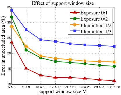
(a) Support window size

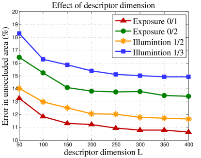
(b) Descriptor dimension

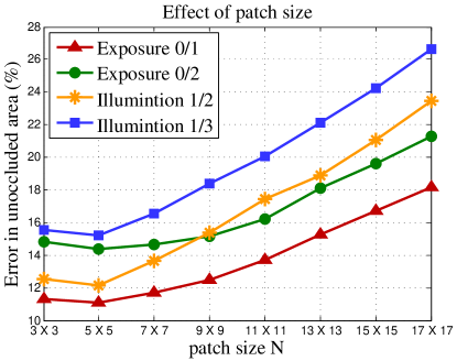
(c) Patch size

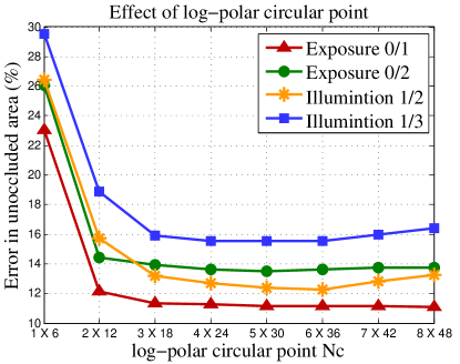
(d) Log-polar circular point

Figure 11: Average bad-pixel error rate on Middlebury benchmark [23] of DASC+LRP descriptor with WTA optimization as varying support window size $M$, descriptor dimension $L$, patch size $N$, and log-polar circular point $N_{c}$ ($\approx N_{\rho}\times N_{\theta}$). In each experiment, all other parameters are fixed as initial values in Sec. 6.1.

6 Experimental Results and Discussions

6.1 Experimental Environments

In experiments, the DASC descriptor was implemented with the following same parameter settings for all datasets: $\{\sigma_{c},\tau_{c},N,M,L^{\mathrm{dasc}}\}=\{0.5,0.03,5\times 5,31\times 31,128\}$ where $M$ is the support window size, and $\{N_{\rho},N_{\theta}\}=\{4,36\}$ for candidate sampling patterns. We set the smoothness parameter $\epsilon=0.03^{2}$ in the GF [20]. For the GI-DASC, the following parameters were used for all datasets: $\{N^{\mathrm{wmsd}}_{\rho},N^{\mathrm{wmsd}}_{\theta},N_{k},o,{\lambda_{c}},{\lambda_{p}}\}=\{3,12,4,10,0.1,30\}$. The number of superpixels is set to about $500$. We implemented the DASC and GI-DASC descriptor in C++ on Intel Core i$7$-$3770$ CPU at $3.40$ GHz.

The DASC descriptor was evaluated with other state-of-the-art descriptors, e.g., SIFT [26], DAISY [12], BRIEF [27], and LSS [17], and other area-based approaches, e.g., ANCC [40], MI+SIFT [38], and RSNCC [8]. We also compared the DASC using a randomized pooling (DASC+RP) with the DASC using a learned randomized pooling (DASC+LRP). Furthermore, the state-of-the-art geometry robust methods such as SID [46], SegSID [46], SegSF [47], GPM [44], DSP [14], and SSF [43] were also compared to the GI-DASC descriptor. For learning the DASC, we built training sets $\mathcal{P}$ from benchmark databases used in each experiment, and these training sets were excluded from experiments.

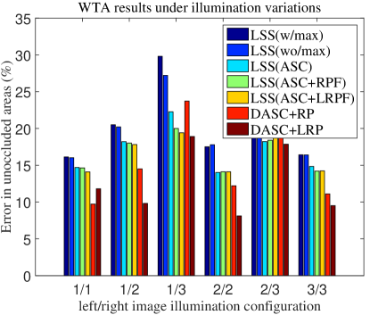
(a) Illumination variation

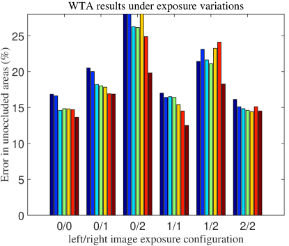
(b) Exposure variation

Figure 12: Average bad-pixel error rate for original LSS [17], LSS without max-pooling, LSS with ASC, LSS using randomized-pooling with fixed center pixel, and the DASC descriptor on Middlebury benchmark [23].

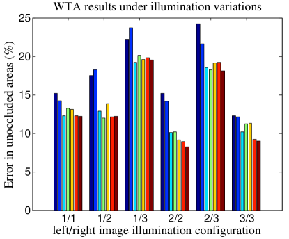
(a) Illumination variation

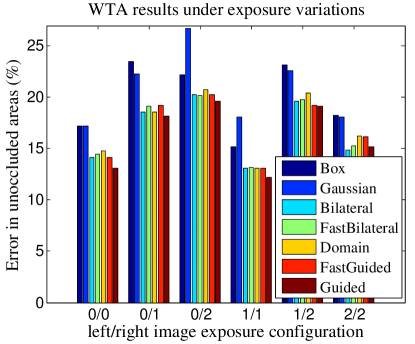
(b) Exposure variation

Figure 13: Average bad-pixel error rate for the DASC descriptor as varying EAF including Box, Gaussian, Bilateral [61], FastBilateral [53], Domain Transform [54], FastGF [62], and GF [20] on Middlebury benchmark [23].

6.2 Parameter and Component Analysis

6.2.1 Parameter sensitivity analysis

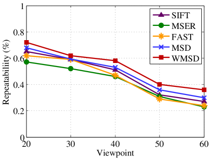
(a) Graffiti

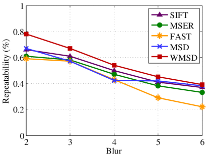
(b) Trees

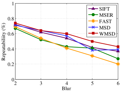
(c) Bikes

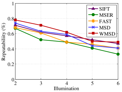
(d) Leuven

Figure 14: Evaluation of the WMSD detection compared to conventional feature detections, such as SIFT [26], MSER [63], FAST [64], and MSD [58]. The WMSD provides reliable feature detection performance, thus providing reliable hypothesis for initial sparse geometric fields.

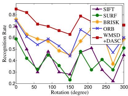
Figure 15: Evaluation of the WMSD detection compared to conventional rotation estimations. Compared to conventional gradient-based rotation estimation (SIFT [26] and SURF [65]) or intensity-based rotation estimation (BRISK [66] and ORB [67]), our WMSD-based rotation estimation (with the DASC descriptor) shows the best performance.

Fig. 11 intensively analyzed the performance of the DASC descriptor as varying associated parameters, including support window size $M$, descriptor dimension $L^{\mathrm{dasc}}$, patch size $N$, and the number of log-point circular point $N_{c}$. To evaluate the quantitative performance, we measured an average bad-pixel error rate on Middlebury benchmark [23]. The larger the support window size $M$, the matching quality is improved but the accuracy gain is saturated around $31\times 31$. Using a larger descriptor dimension $L^{\mathrm{dasc}}$ yields a better performance since the descriptor encodes more information. Considering the trade-off between efficiency and robustness, $L^{\mathrm{dasc}}=128$ is set in experiments. When the patch size $N$ increases, the matching quality is degraded since a series of similarity values measured with large patches may lose locally discriminative details. The number of log-polar circular point $N_{c}$ does not affect the performance much, since optimal patterns can be sampled even from small $N_{c}$.

6.2.2 Component-wise performance gain analysis

The DASC is originally motivated by the LSS concept from [17]. The DASC consists of three key ingredients: adaptive self-correlation (ASC), randomized pooling (RP), and learning sampling pattern. In this context, we analyzed an accuracy gain of the DASC over the LSS on the Middlebury benchmark as shown in Fig. 12. Note that all experiments were done using LSS without max pooling, ‘LSS(wo/max)’. The original LSS method [17] uses the SSD for measuring the patch similarity. We replaced the patch similarity of the LSS method with the ASC, named ‘LSS(ASC)’, and then measured its matching accuracy. As expected, the ASC improves the performance compared to the SSD used in the original LSS. We also evaluated the LSS using a randomized pooling with fixed center pixel, ‘LSS(ASC+RPF)’, and the LSS using a learned randomized pooling with fixed center pixel, ‘LSS(ASC+LRPF)’. Unlike center-biased poolings, the DASC chooses sampling patterns randomly (‘DASC+RP’), improving the performance. Using learned sampling patterns (‘DASC+LRP’) also leads to a performance gain.

TABLE I: Evaluation of computational time. The brute-force and efficient computation of the DASC is denoted as †and ‡, respectively.

image size	SIFT	DAISY	LSS	DASC†	DASC‡
$463\times 370$	$130.3s$	$2.5s$	$31s$	$128s$	$1.3s$
$800\times 600$	$252s$	$3.8s$	$59s$	$256s$	$2.1s$

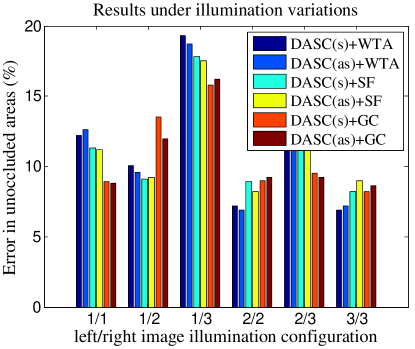
(a) Illumination variation

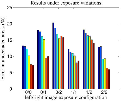
(b) Exposure variation

Figure 16: Evaluation of a symmetric measure $\Psi(i,j)$ and an asymmetric measure $\tilde{\Psi}(i,j)$ in the DASC as varying optimization schemes with WTA, SF [13], and GC [68]. It shows that there are no significant performance gaps when using symmetric and asymmetric measure.

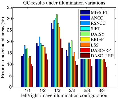
(a) Illumination variation

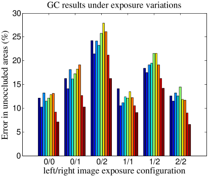
(b) Exposure variation

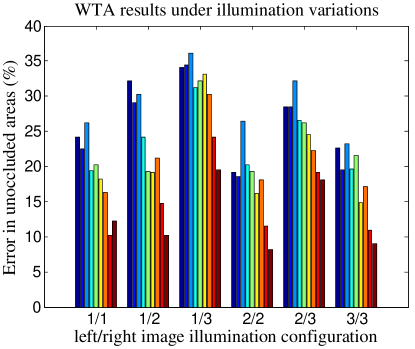
(c) Illumination variation

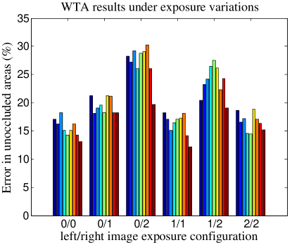
(d) Exposure variation

Figure 17: Average bad-pixel error rate on Middlebury benchmark with illumination variations and exposure variations. The GC (first row) and WTA (second row) were used for optimization, respectively. Our DASC+LRP shows the best performance with the lowest error rate.

6.2.3 Edge-aware filtering analysis

In Fig. 13, we analyzed the performance of the DASC descriptor when different EAF is employed for computing $\omega_{i,i^{\prime}}$. When using a simple, unweighted ‘Box’ filtering ($\omega_{i,i^{\prime}}=1$), the patch similarity (7) becomes a normalized cross-correlation (NCC). In the Box and Gaussian filtering case, there exists a performance limitation. In contrast, all EAF methods show a satisfactory performance, including the bilateral filter [61], the fast bilateral filter [57], the domain transform [54], the fast GF [62], and GF [69]. In experiments, we utilized the GF [69].

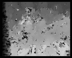
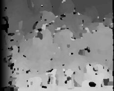
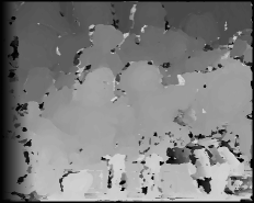
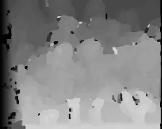
(a) Left image

(b) Right image

(c) ANCC [40]

(d) BRIEF [27]

(e) SIFT [26]

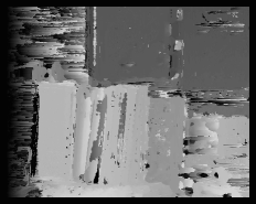
(f) LSS [17]

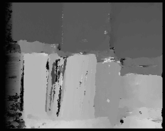
(g) DASC+LRP

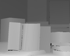
(h) Ground Truth

Figure 18: Comparison of disparity estimation for Dolls and Books image pairs under illumination combination ‘1/3’ and exposure combination ‘0/2’, respectively. Compared to other approaches, our DASC descriptor estimates accurate and edge-preserved disparity maps while reducing artifacts.

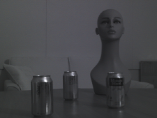
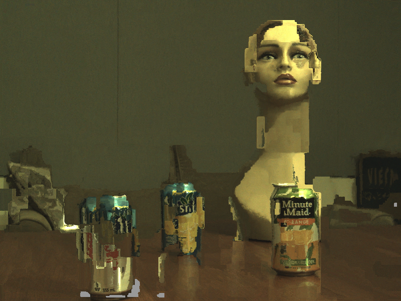
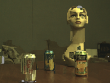
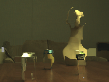
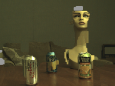
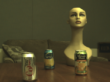
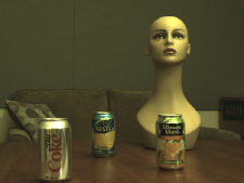
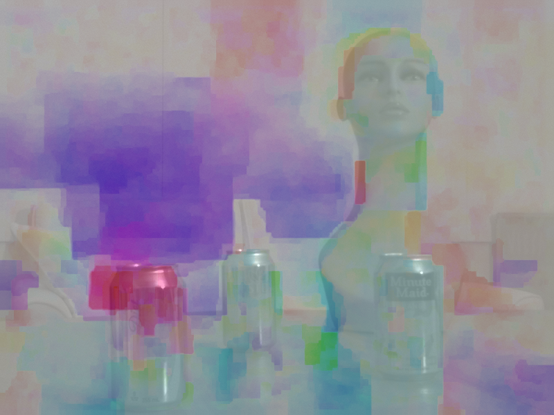
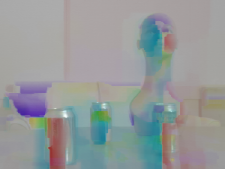
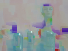
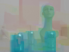
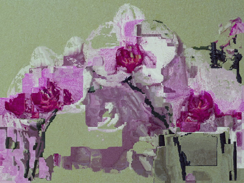
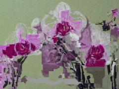
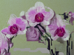
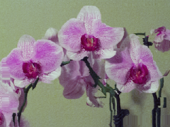
(a) Image pairs

(b) MI+SIFT [38]

(c) BRIEF [27]

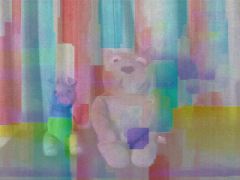
(d) DAISY [12]

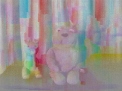
(e) SIFT [26]

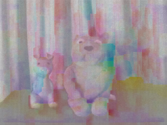
(f) LSS [17]

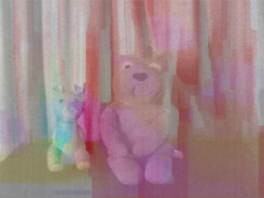
(g) DASC+RP

(h) DASC+LRP

Figure 19: Comparison of dense correspondence for (from top to bottom) RGB-NIR images and flash-noflash images. The results consist of warped color images and correspondence flow fields overlaid with reference images. Compared to other conventional approaches, our DASC+LRP descriptor estimates reliable dense correspondence fields for challenging multi-modal and multi-spectral image pairs.

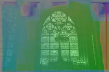
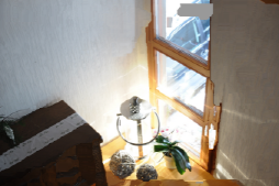
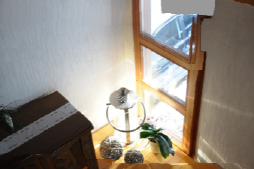
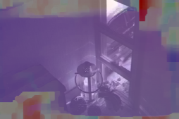
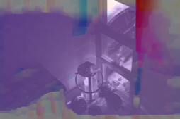
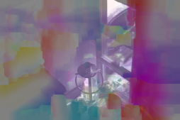
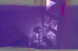
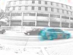
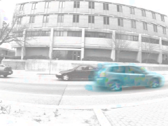
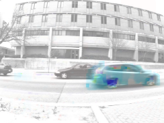
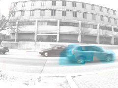
(a) Image pairs

(b) RSNCC [8]

(c) BRIEF [27]

(d) DAISY [12]

(e) SIFT [26]

(f) LSS [17]

(g) DASC+RP

(h) DASC+LRP

Figure 20: Comparison of dense correspondence for (from top to bottom) different exposure images and blurred-sharpen images. The results consist of warped color images and correspondence flow fields overlaid with reference images. Compared to other conventional approaches, our DASC+LRP descriptor estimates reliable dense correspondence fields for challenging multi-modal and multi-spectral image pairs.

6.2.4 WMSD feature detector analysis

In Fig. 14 and Fig. 15, we analyzed the feature detection performance of the WMSD detector with a repeatability [64] and recognition rate measure [27] in Mikolajczyk dataset [70]. Compared to conventional feature detection approaches [26, 63, 64, 58], the WMSD detector extracts reliable and distinctive points with a high repeatability thanks to its robustness for modality variations including blur artifacts and illumination changes. Furthermore, compared to conventional gradient-based [26, 65] or intensity-based rotation estimations [66, 67], our WMSD-based rotation estimation combined with the DASC descriptor shows the best performance with a high recognition rate.

6.2.5 Symmetric and asymmetric measure analysis

As shown in Fig. 16, a performance gap between using the asymmetric measure $\tilde{\Psi}(i,j)$ in (9) and the symmetric measure $\Psi(i,j)$ in (7) is negligible, while using the asymmetric measure is much faster.

6.2.6 Runtime analysis

In Table I, we compared the computational speed of DASC descriptor with state-of-the-art local descriptors, SIFT [26], DAISY [12], and LSS [17]. The DASC provides state-of-the-art computational speed. It should be noted that through recent more efficient edge-aware filters [62], the runtime of DASC can be further reduced.

6.3 Middlebury Stereo Benchmark

We evaluated our DASC+LRP descriptor compared to other approaches in Middlebury stereo benchmark containing illumination and exposure variations [23]. In experiments, the illumination (or exposure) combination ‘1/3’ indicates that two images were captured under $1^{st}$ and $3^{rd}$ illumination (exposure) conditions, respectively [23]. Fig. 17 shows average bad matching errors in un-occluded areas of depth maps obtained under illumination or exposure variations with the graph-cut (GC) [68] and winner-takes-all (WTA) optimization. Fig. 18 shows disparity maps for severe illumination variations obtained by varying cost functions with the WTA optimization. Our DASC+LRP descriptor achieves the best results both quantitatively and qualitatively. Area-based approaches, e.g., MI+SIFT [38], ANCC [40], and RSNCC [8], are very sensitive to severe radiometric variations, especially when local variations frequently occur. Contrarily, descriptor-based approaches perform better than the area-based approaches. Interestingly, the BRIEF [27] is better than other gradient-based descriptors (SIFT [26] and DAISY [12]) thanks to an ordering robustness.

6.4 Multi-modal and Multi-spectral Benchmark

Next, we evaluated our DASC+LRP descriptor with images under modality variations, e.g., RGB-NIR [8, 1], different exposure [8, 7], flash-noflash [7], and blurred artifacts [5, 6]. As varying descriptors and similarity measures, we use the WTA and SIFT flow optimization using the hierarchical dual-layer belief propagation (BP) [13], whose code is publicly available. Unlike the Middlebury stereo benchmark, these datasets have no ground truth correspondence maps, and thus we manually obtained ground truth displacement vectors for $100$ corner points for all images, and used them for an objective evaluation similar to [8].

Area-based approaches, e.g., MI+SIFT [38], ANCC [40], and RSNCC [8], are very sensitive to local variations. As already described in literatures [8], gradient-based approaches, e.g., SIFT [26] and DAISY [12], have shown limited performance in RGB-NIR pairs where the gradient reversal and inversion frequently appear. The BRIEF [27] cannot deal with noisy and modality varying regions since it considers a pixel difference only. It should be noted that some efforts have been made to estimate reliable flow maps in the motion blur, e.g., blur-flow [71], but they typically employ an iterative matching framework, which relies heavily on an initial estimate. Additionally, they do not scale well to general purpose matching scenarios. Unlike these approaches, the LSS [17] and our descriptor consider the local self-similarities, but the LSS still lacks a discriminative power for dense matching. Our DASC+RP descriptor leveraging patch-wise pooling with adaptive self-correlation provides satisfactory results under modality variations. By employing the optimal sampling pattern via discriminative learning (DASC+LRP), the matching accuracy was further improved. Fig. 19 and Fig. 20 show qualitative evaluation, clearly demonstrating the outstanding performance of our descriptor. Table II shows an objective evaluation of DASC+LRP descriptor and other state-of-the-art methods on these datasets.

TABLE II: Comparison of quantitative evaluation on multi-spectral and multi-modal images.

	WTA optimization					SF optimization [13]
	RGB-NIR	flash-noflash	diff. expo.	blur-sharp	Average	RGB-NIR	flash-noflash	diff. expo.	blur-sharp	Average
MI+SIFT [38]	25.13	27.12	28.23	24.21	27.12	17.21	13.24	14.16	20.14	16.87
ANCC [40]	23.21	20.42	25.19	26.14	23.74	18.45	14.14	11.96	19.24	15.94
RSNCC [8]	27.51	25.12	18.21	27.91	24.68	13.41	15.87	9.15	18.21	14.16
SIFT [26]	24.11	18.72	19.42	27.18	22.36	18.51	11.06	14.87	20.78	16.35
DAISY [12]	27.61	26.30	20.72	27.41	25.51	20.42	10.84	12.71	22.91	16.72
BRIEF [27]	29.14	18.29	17.13	26.43	22.75	17.54	9.21	9.54	19.72	14.05
LSS [17]	27.82	19.18	18.21	26.14	22.84	16.14	11.88	9.11	18.51	13.91
DASC+RP	18.21	14.28	12.12	17.11	12.18	15.43	7.51	7.32	12.21	9.68
DASC+LRP	13.42	11.28	9.23	13.28	11.80	8.10	5.41	6.24	10.81	7.64

6.5 DIML Multi-modal Benchmark

Since there have been no database with both photometric and geometric variations, we built the DIML multi-modal benchmark [25]. All databases were taken by SONY Cyber-Shot DSC-RX100 camera in a darkroom with the lighting booth GretagMacbeth SpectraLight III. In terms of geometric deformations, we captured 10 geometry image sets by combining geometric variations of viewpoint, scale, and rotation as shown in Fig. 21, and each image set consists of images taken under $5$ different photometric variation pairs including illumination, exposure, flash-noflash, blur, and noise as shown in Fig. 22. Therefore, the DIML multi-modal benchmark consists of $100$ images with the size of $1200\times 800$. Furthermore, by following [13], we manually built ground truth object annotation maps to evaluate the performance quantitatively, and computed the label transfer accuracy (LTA) $\mathcal{A}^{\mathrm{LTA}}$ such that

$$\mathcal{A}^{\mathrm{LTA}}=\frac{1}{\mathcal{T}_{a}}\sum\nolimits_{i\in{\mathcal{I}}}{1({e_{i}}\neq{a_{i}},{a_{i}}>0)}$$ (20)

where the ground-truth annotation is ${a_{i}}$, estimated annotation is ${e_{i}}$, and $\mathcal{T}_{a}=\sum\nolimits_{i\in{\mathcal{I}}}{1({a_{i}}>0)}$ is the number of labeled pixels. This metric has been widely used in wide-baseline matching tasks [14]. Though $\mathcal{A}^{\mathrm{LTA}}$ does not measure a matching performance in a pixel precision, it was shown in [13] that this metric is an excellent alternative enough to evaluate the performance of descriptors in case that there are no ground truth correspondence maps available.

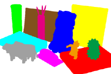
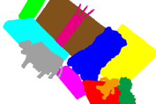
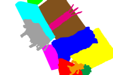
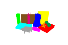
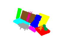
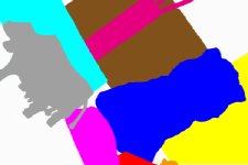
Figure 21: Examples of DIML multi-modal benchmark. It consists of images taken under $10$ different geometric conditions such as viewpoint, scale, rotation, and scale-rotation with ground truth annotation.

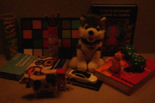
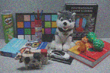
Figure 22: Examples of DIML multi-modal benchmark. Each geometry image sets in Fig. 21 consists of $5$ different photometric variations such as illumination, exposure, flash-noflash, blur, and noise.

(a) DAISY [12]

(b) LSS [17]

(c) SegSIFT [47]

(d) SegSID [47]

(e) DSP [14]

(f) SSF [43]

(g) DASC

(h) GI-DASC

Figure 23: Comparison of quantitative evaluation on DIML benchmark [25]. Each result represents the LTA for geometric (x-axis) and photometric (y-axis) variations, respectively. The DASC outperforms conventional descriptors such as DAISY [12] and LSS [17]. Interestingly, its accuracy is also higher than those of state-of-the-art geometry-invariant methods including SegSIFT [47], SegSID [47], DSP [14], and SSF [43]. The GI-DASC shows the best performance under varying photometric and geometric conditions.

For an image from the reference geometry image set (the first image in Fig. 21), we estimated visual correspondence maps with images from other geometry image set, and then computed the LTA. Furthermore, visual correspondence maps were estimated for each photometric pair. Here, matching results at occluded pixels should be excluded in the evaluation as they have no corresponding pixels. We hence warped an image taken from near into an image taken at a distance, when computing the LTA. The experimental setup for DIML multi-modal benchmark was given in detail at our project page [25].

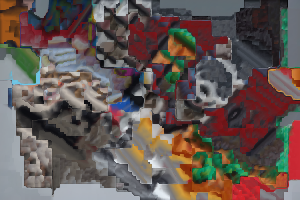
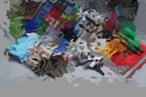
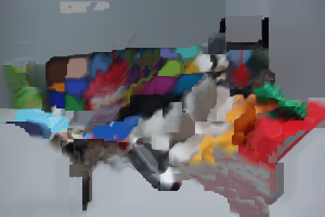
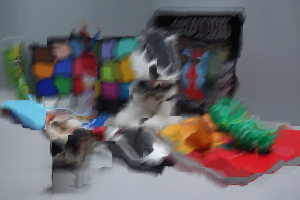
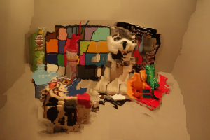
(a) Image pairs

(b) DAISY [12]

(c) Seg-SIFT [47]

(d) Seg-SID [46]

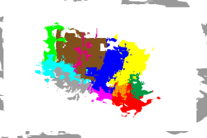
(e) DSP [14]

(f) SSF [43]

(g) DASC

(h) GI-DASC

Figure 24: Comparison of qualitative evaluation on DIML multi-modal benchmark. The results consist of warped color images and warped ground truth annotations. Compared to other conventional descriptors and geometry-invariant approaches, our DASC descriptor estimates reliable dense correspondence fields for image pairs across varying geometric and photometric conditions.

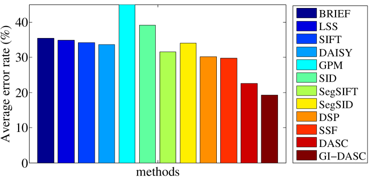
Figure 25: Average error rates on DIML multi-modal benchmark.

We compared our two descriptors, DASC and GI-DASC, with conventional descriptors such as SIFT [26], DAISY [12], BRIEF [27], and LSS [17], and state-of-the-arts geometry-invariant approaches such as SID [46], SegSIFT [47], SegSID [47], GPM [44], DSP [14], and SSF [43]. For the sake of simplicity, we omit ‘LRP’ in the DASC-LRP and GI-DASC-LRP. Fig. 23 shows the LTA error rates as varying photometric and geometric deformations. Fig. 24 shows qualitative evaluation results. As expected, feature descriptors such as SIFT [26], DAISY [12], BRIEF [27], and LSS [17], though using a powerful global optimization, i.e., hierarchical dual-layer BP [13], exhibit limitations on severe geometric variations, while they provide robustness to some extent for photometric variations. Our DASC descriptor in Fig. 23(k) shows a better performance than other descriptors, but it also shows the limitation for severe geometric variations. The GPM [44] had very low performance in terms of flow estimation although it provides plausible warping results. The SID [46] have been proposed to provide geometric robustness, but it is unable to address photometric variations. Segmentation-aware description [47] could improve the matching accuracy of SIFT and SID for geometric variations, but it also has limitation since it also reduces a discriminative power of descriptor itself as shown in Fig. 23(g) and (h). The DSP [14] provides limited performances, since it just uses the SIFT with a fixed scale and rotation. The SSF [43] estimates visual correspondence by repeatedly applying the SIFT on the scale-space while enduring a huge computational complexity, but it still has limitations in terms of computational complexity. Contrarily, the GI-DASC descriptor optimized by hierarchical dual-layer BP [13] provides the robustness for both photometric and geometric deformations as shown in Fig. 23(l). Fig. 26 shows the average error rates on DIML multi-modal benchmark.

6.6 MPI Optical Flow Benchmark

Optical flow methods typically assume only a small displacement between consecutive frames. Several approaches have been proposed to estimate a large displacement flow vector [72]. However, motion blur and illumination variation can degenerate the performance of these approaches. In order to handle such challenging issues simultaneously, we applied the DASC to the large displacement optical flow (LDOF) approach [72]. It was evaluated on the MPI SINTEL database [10] containing large non-rigid motion as well as specular reflections, motion blur, and defocus blur. The dataset consists of two kind of rendering frames, named clean and final pass, and each set contains $12$ sequences with over $500$ frames in total [10]. Table III shows average end-point error (EPE) results on MPI SINTEL. The DASC achieves a higher gain, compared to other descriptors.

TABLE III: Comparison of average EPE on the MPI SINTEL [10].

	Clean Pass		Final Pass
	all	unmatched	all	unmatched
Classic-NL [11]	7.940	39.821	9.439	43.123
LDOF [72]	7.180	38.124	8.422	42.892
LDOF+BRIEF [27]	6.281	37.841	7.741	41.875
LDOF+LSS [17]	6.182	37.514	7.152	40.332
LDOF+DASC	5.578	36.975	6.384	38.932

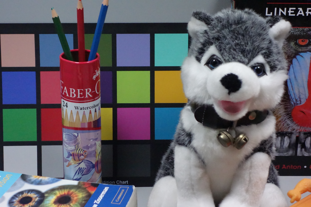
(a) image 1

(b) image 2

(c) SSF [43]

(d) GI-DASC

Figure 26: Limitations for images under severe geometric variations.

6.7 Limitations

Similar to [42, 43, 21], our GI-DASC approximately determines a relative scale using successive Gaussian smoothing, which might work in only a limited range of scale variation as in Fig. 26. By leveraging an octave structure based on sub-sampling [26], a wider range of scale may be covered.

7 Conclusion

The robust novel dense descriptor called the DASC has been proposed for dense multi-spectral and multi-modal correspondences. It leverages an adaptive self-correlation measure and a randomized receptive field pooling learned by linear discriminative learning. Moreover, by making use of fast edge-aware filters, our DASC descriptor is capable of computing the dense descriptor very efficiently. In order to address geometric variations, the GI-DASC descriptor also has been proposed by leveraging the efficiency and effectiveness of the DASC through a superpixel-based representation. The DASC and GI-DASC descriptor demonstrated its robustness in establishing dense correspondence between challenging image pairs taken under different modality conditions, e.g., RGB-NIR, different illumination and exposure, flash-noflash, blurring artifacts. We believe our method will serve as an essential tool for several applications using multi-modal and multi-spectral images.

References

- [1] M. Brown and S. Susstrunk, “Multispectral sift for scene category recognition,” In Proc. of CVPR, 2011.
- [2] Q. Yan, X. Shen, L. Xu, and S. Zhuo, “Cross-field joint image restoration via scale map,” In Proc. of ICCV, 2013.
- [3] D. Krishnan and R. Fergus, “Dark flash photography,” In Proc. of ACM SIGGRAGH, 2009.
- [4] G. Petschnigg, M. Agrawals, and H. Hoppe, “Digital photography with flash and no-flash iimage pairs,” In Proc. of ACM SIGGRAGH, 2004.
- [5] Y. HaCohen, E. Shechtman, and E. Lishchinski, “Deblurring by example using dense correspondence,” In Proc. of ICCV, 2013.
- [6] H. Lee and K. Lee, “Dense 3d reconstruction from severely blurred images using a single moving camera,” In Proc. of CVPR, 2013.
- [7] P. Sen, N. K. Kalantari, M. Yaesoubi, S. Darabi, D. B. Goldman, and E. Shechtman, “Robust patch-based hdr reconstruction of dynamic scenes,” In Proc. of ACM SIGGRAGH, 2012.
- [8] X. Shen, L. Xu, Q. Zhang, and J. Jia, “Multi-modal and multi-spectral registration for natural images,” In Proc. of ECCV, 2014.
- [9] D. Scharstein and R. Szeliski, “A taxonomy and evaluation of dense two-frame stereo correspondence algorithms,” IJCV, vol. 47, no. 1, pp. 7–42, 2002.
- [10] D. Butler, J. Wulff, G. Stanley, and M. Black, “A naturalistic open source movie for optical flow evaluation,” In Proc. of ECCV, 2012.
- [11] D. Sun, S. Roth, and M. Black, “Secret of optical flow estimation and their principles,” In Proc. of CVPR, 2010.
- [12] E. Tola, V. Lepetit, and P. Fua, “Daisy: An efficient dense descriptor applied to wide-baseline stereo,” IEEE Trans. PAMI, vol. 32, no. 5, pp. 815–830, 2010.
- [13] C. Liu, J. Yuen, and A. Torralba, “Nonparametric scene parsing via label transfer,” IEEE Trans. PAMI, vol. 33, no. 12, pp. 2368–2382, 2011.
- [14] J. Kim, C. Liu, F. Sha, and K. Grauman, “Deformable spatial pyramid matching for fast dense correspondences,” In Proc. of CVPR, 2013.
- [15] Y. Li, D. Min, M. S. Brown, M. N. Do, and J. Lu, “Spm-bp: Sped-up patchmatch belief propagation for continuous mrfs,” In Proc. of ICCV, 2015.
- [16] P. Pinggera, T. Breckon, and H. Bischof, “On cross-spectral stereo matching using dense gradient features,” In Proc. of BMVC, 2012.
- [17] E. Schechtman and M. Irani, “Matching local self-similarities across images and videos,” In Proc. of CVPR, 2007.
- [18] P. Heinrich, M. Jenkinson, M. Bhushan, T. Matin, V. Gleeson, S. Brady, and A. Schnabel, “Mind: Modality indepdent neighbourhood descriptor for multi-modal deformable registration,” Medi. Image Anal., vol. 16, no. 3, pp. 1423–1435, 2012.
- [19] A. Torabi and G. Bilodeau, “Local self-similarity-based registration of human rois in pairs of stereo thermal-visible videos,” Pattern Recognition, vol. 46, no. 2, pp. 578–589, 2013.
- [20] K. He, J. Sun, and X. Tang, “Guided image filtering,” IEEE Trans. PAMI, vol. 35, no. 6, pp. 1397–1409, 2013.
- [21] H. Yang, W. Lin, and J. Lu, “Daisy filter flow: A generalized discrete approach to dense correspondences,” In Proc. of CVPR, 2014.
- [22] J. Hur, H. Lim, C. Park, and S. C. Ahn, “Generalized deformable spatial pyramid: Geometry-preserving dense correspondence estimation,” In Proc. of CVPR, 2015.
- [23] http://vision.middlebury.edu/stereo/.
- [24] S. Kim, D. Min, B. Ham, S. Ryu, M. N. Do, and K. Sohn, “Dasc: Dense adaptive self-correlation descriptor for multi-modal and multi-spectral correspondence,” In Proc. of CVPR, 2015.
- [25] http://diml.yonsei.ac.kr/srkim/DASC/.
- [26] D. Lowe, “Distinctive image features from scale-invariant keypoints,” IJCV, vol. 60, no. 2, pp. 91–110, 2004.
- [27] M. Calonder, “Brief : Computing a local binary descriptor very fast,” IEEE Trans. PAMI, vol. 34, no. 7, pp. 1281–1298, 2011.
- [28] A. Alahi, R. Ortiz, and P. Vandergheynst, “Freak : Fast retina keypoint,” In Proc. of CVPR, 2012.
- [29] S. Saleem and R. Sablatnig, “A robust sift descriptor for multispectral images,” IEEE SPL, vol. 21, no. 4, pp. 400–403, 2014.
- [30] Y. Ye and J. Shan, “A local descriptor based registration method for multispectral remote sensing images with non-linear intensity differences,” ISPRS J. Photogram. Remote Sens., vol. 90, no. 7, pp. 83–95, 2014.
- [31] K. Alex, S. Ilya, and E. H. Geoffrey, “Imagenet classification with deep convolutional neural networks,” In Proc. of NIPS, 2012.
- [32] K. Simonyan, A. Vedaldi, and A. Zisserman, “Learning local feature descriptors using convex optimisation,” IEEE Trans. PAMI, vol. 36, no. 8, pp. 1573–1585, 2014.
- [33] P. Fischer, A. Dosovitskiy, and T. Brox, “Descriptor matching with convolutional neural networks: A comparison to sift,” arXiv:1405.5769, 2014.
- [34] J. Donahue, Y. Jia, O. Vinyals, J. Hoffman, N. Zhang, E. Tzeng, and T. Darrell, “Decaf: A deep convolutional activation feature for generic visual recognition,” In Proc. of ICML, 2014.
- [35] E. Simo-Serra, E. Trulls, L. Ferraz, I. Kokkinos, P. Fua, and F. Moreno-Noguer, “Discriminative learning of deep convolutional feature point descriptors,” In Proc. of ICCV, 2015.
- [36] J. Dong and S. Soatto, “Domain-size pooling in local descriptors: Dsp-sift,” In Proc. of CVPR, 2015.
- [37] J. Pluim, J. Maintz, and M. Viergever, “Mutual information based registration of medical images: A survey,” IEEE Trans. MI, vol. 22, no. 8, pp. 986–1004, 2003.
- [38] Y. Heo, K. Lee, and S. Lee, “Joint depth map and color consistency estimation for stereo images with different illuminations and cameras,” IEEE Trans. PAMI, vol. 35, no. 5, pp. 1094–1106, 2013.
- [39] J. Xu, Q. Yang, J. Tang, and Z. Feng, “Linear time illumination invariant stereo matching,” IJCV, 2016.
- [40] Y. Heo, K. Lee, and S. Lee, “Robust stereo matching using adaptive normalized cross-correlation,” IEEE Trans. PAMI, vol. 33, no. 4, pp. 807–822, 2011.
- [41] M. Irani and P. Anandan, “Robust multi-sensor image alignment,” In Proc. of ICCV, 1998.
- [42] T. Hassner, V. Mayzels, and L. Zelnik-Manor, “On sifts and their scales,” In Proc. of CVPR, 2012.
- [43] W. Qiu, X. Wang, X. Bai, A. Yuille, and Z. Tu, “Scale-space sift flow,” In Proc. of WACV, 2014.
- [44] C. Barnes, E. Shechtman, D. B. Goldman, and A. Finkelstein, “The generalized patchmatch correspondence algorithm,” In Proc. of ECCV, 2010.
- [45] J. Lu, H. Yang, D. Min, and M. N. Do, “Patchmatch filter: Efficient edge-aware filtering meets randomized search for fast correspondence field estimation,” In Proc. of CVPR, 2013.
- [46] I. Kokkinos and A. Yuille, “Scale invariance without scale selection,” In Proc. of CVPR, 2008.
- [47] E. Trulls, I. Kokkinos, A. Sanfeliu, and F. M. Noguer, “Dense segmentation-aware descriptors,” In Proc. of CVPR, 2013.
- [48] R. Zabih and J. Woodfill, “Non-parametric local transforms for computing visual correspondence,” In Proc. of ECCV, 1994.
- [49] B. Fan, Q. Kong, T. Trzcinski, and Z. Wang, “Receptive fields selection for binary feature description,” IEEE Trans. IP, vol. 23, no. 6, pp. 2583–2595, 2014.
- [50] C. Chang and C. Lin, “Libsvm: A library for support vector machines,” ACM Trans. IST, vol. 2, no. 3, pp. 1–27, 2011.
- [51] C. Lee, A. Bhardwaj, V. Jagadeesh, and R. Piramuthu, “Region-based discriminative feature pooling for scene text recognition,” In Proc. of CVPR, 2014.
- [52] T. Trzcinski, M. Christoudias, and V. Lepetit, “Learning image descriptor with boosting,” IEEE Trans. PAMI, vol. 37, no. 3, pp. 597–610, 2015.
- [53] Q. Yang, K. Tan, and N. Ahuja, “Real-time o(1) bilateral filtering,” In Proc. of CVPR, 2009.
- [54] E. Gastal and M. Oliveira, “Domain transform for edge-aware image and video processing,” In Proc. of ACM SIGGRAGH, 2011.
- [55] M. J. Black, G. Sapiro, D. H. Marimont, and D. Heeger, “Robust anisotropic diffusion,” IEEE Trans. IP, vol. 7, no. 3, pp. 421–432, 1998.
- [56] C. Rhemann, A. Hosni, M. Bleyer, C. Rother, and M. Gelautz, “Fast cost-volume filtering for visual correspondence and beyond,” In Proc. of CVPR, 2011.
- [57] S. Paris and F. Durand, “A fast approximation of the bilateral filter using a signal processing approach,” IJCV, vol. 81, no. 1, pp. 24–52, 2009.
- [58] F. Rombari and L. D. Stefano, “Interest points via maxiaml self-dissimilarities,” In Proc. of ACCV, 2014.
- [59] S. Kim, B. Ham, S. Ryu, S. J. Kim, and K. Sohn, “Robust stereo matching using probabilistic laplacian surface propagation,” In Proc. of ACCV, 2014.
- [60] M. Lang, O. Wang, T. Aydic, A. Smolic, and M. Gross, “Practical temporal consistency for image-based graphics applications,” In Proc. of SIGGRAPH, 2012.
- [61] C. Tomasi and R. Manduchi, “Bilateral filtering for gray and color images,” In Proc. of ICCV, 1998.
- [62] K. He and J. Sun, “Fast guided filter,” arXiv:1505.00996, 2015.
- [63] J. Matas, O. Chum, and T. Urban, M. amd Pajdla, “Robust wide baseline stereo from maximally stable extremal regions,” In Proc. of BMVC, 2002.
- [64] E. Rosten, R. Porter, and T. Drummond, “Faster and better: a machine learning approach to corner detection,” IEEE Trans. PAMI, vol. 32, no. 1, pp. 105–119, 2010.
- [65] H. Bay, T. Tuytelaars, and L. V. Gool, “Surf: Speeded up robust features,” In Proc. of ECCV, 2006.
- [66] S. Leutenegger, M. Chli, and R. Siegwart, “Brisk : Binary robust invariant scalable keypoints,” In Proc. of ICCV, 2011.
- [67] E. Rublee, V. Rabaud, K. Konolige, and G. Bradski, “Orb: an efficient alternative to sift or surf,” In Proc. of ICCV, 2011.
- [68] Y. Boykov, O. Yeksler, and R. Zabih, “Fast approximation enermgy minimization via graph cuts,” IEEE Trans. PAMI, vol. 23, no. 11, pp. 1222–1239, 2001.
- [69] K. He, J. Sun, and X. Tang, “Guided image filtering,” In Proc. of ECCV, 2010.
- [70] K. mikolajczyk, T. Tuytelaars, C. Schmid, A. Zisserman, J. Matas, F. Schaffalitzky, T. Kadir, and L. V. Gool, “A comparison of affine region detectors,” IJCV, vol. 65, no. 1, pp. 43–72, 2005.
- [71] T. Portz, L. Zhang, and H. Jiang, “Optical flow in the presence of spatially-varying motion blur,” In Proc. of CVPR, 2012.
- [72] T. Brox and J. Malik, “Large displacement optical flow: Descriptor matching in variational motion estimation,” IEEE Trans. PAMI, vol. 33, no. 3, pp. 500–513, 2011.