Estimate of the radius responsible for quasinormal modes in the extreme Kerr limit and asymptotic behavior of
the Sasaki–Nakamura transformation

Abstract

The Sasaki–Nakamura transformation gives a short-ranged potential and a convergent source term for the master equation of perturbations in the Kerr space-time. In this paper, we study the asymptotic behavior of the transformation, and present a new relaxed necessary and sufficient condition for the transformation to obtain the short-ranged potential in the assumption that the transformation converges in the far distance. Also, we discuss the peak location of the potential which is responsible for quasinormal mode frequencies in tWKB analysis. Finally, in the extreme Kerr limit, $a/M\to 1$, where $M$ and $a$ denote the mass and spin parameter of a Kerr black hole, respectively, we find the peak location of the potential, $r_{\rm p}/M\lesssim 1+1.8\,(1-a/M)^{1/2}$ by using the new transformation. The uncertainty of the location is as large as that expected from the equivalence principle.

E31, E02, E01, E38

1 Introduction

The source of GW150914, a gravitational wave (GW) event observed by advanced LIGO on September 14, 2015 Abbott:2016blz , is considered as a merging binary black hole (BBH) and the black hole (BH) masses are estimated as $36^{+5}_{-4}M_{\odot}$ and $29^{+4}_{-4}M_{\odot}$, respectively. According to Ref. TheLIGOScientific:2016htt , the BH masses are well predicted by the recent population synthesis results of Population III BBHs Kinugawa:2014zha ; Kinugawa:2015nla ; Kinugawa:2016mfs (see also Ref. Hartwig:2016nde ).

The mass and (non-dimensional) spin of the remnant BH were estimated as $62^{+4}_{-4}M_{\odot}$ and $0.67^{+0.05}_{-0.07}$ TheLIGOScientific:2016wfe by using the model derived in Refs. Healy:2014yta ; Ghosh:2015jra , respectively. But, the signal from the ringdown phase of GWs, described by quasinormal modes (QNMs) of a BH, was too weak to test general relativity (see Refs. Berti:2007zu ; Nakano:2015uja , and also Refs. Konoplya:2016pmh ; Yunes:2016jcc ), and only a consistency check for the least-damped QNM has been done in Ref. TheLIGOScientific:2016src . However, since the expected event rate is high Kinugawa:2014zha ; Kinugawa:2015nla ; Kinugawa:2016mfs , and the sensitivities of GW observations will improve, there will be a good chance to have an event with much higher signal-to-noise ratio.

To consider QNMs, we use the BH perturbation approach. The Kerr metric Kerr:1963ud in the Boyer–Lindquist coordinates is written as

$$ds^{2} = -\left(1-\frac{2Mr}{\Sigma}\right)dt^{2}-\frac{4Mar~{}{\rm{sin}^{2}\theta}}{\Sigma}dtd\phi+\frac{\Sigma}{\Delta}dr^{2}$$ (2)

$$+\Sigma d\theta^{2}+\left(r^{2}+a^{2}+\frac{2Ma^{2}r}{\Sigma}\sin^{2}\theta\right)\sin^{2}\theta d\phi^{2}\,,$$

where $\Sigma=r^{2}+a^{2}\cos^{2}\theta$, $\Delta=r^{2}-2Mr+a^{2}$, and $M$ and $a$ denote the mass and the spin parameter of a Kerr BH, respectively. The Kerr space-time is the background to calculate BH perturbations.

Perturbations are discussed by using the Teukolsky formalism. The radial Teukolsky equation Teukolsky:1973ha for gravitational perturbations in the Kerr space-time is formally written as

$$\Delta^{2}\frac{d}{dr}\frac{1}{\Delta}\frac{dR}{dr}-VR=-T\,,$$ (3)

where $T$ is the source and the potential $V$ is given by

$$V=-\frac{K^{2}}{\Delta}-\frac{2iK\Delta^{\prime}}{\Delta}+4iK^{\prime}+\lambda\,,$$ (4)

with

$$K=\left(r^{2}+a^{2}\right)\,\omega-am\,.$$ (5)

The constants $m$ and $\lambda$ in the Teukolsky equation label the spin-weighted spheroidal harmonics $Z^{a\omega}_{\ell m}(\theta,\,\phi)$. $\lambda$ is the separation constant which depends on $m$ and $a\omega$. A prime denotes the derivative with respect to $r$.

There are various modifications of the original Teukolsky equation proposed to improve the behavior of the potential $V$ and the source term $T$. For example, in Ref. Chandrasekhar:1976zz (and related references therein), Chandrasekhar and Detweiler developed various transformations in the 1970s. In Refs. Nakamura:2016gri ; Nakano:2016sgf , we used the Detweiler potential given in Ref. Detweiler:1977gy to study QNM frequencies in WKB analysis Mashhoon:1985cya ; Schutz:1985zz . Sasaki and Nakamura Sasaki:1981kj ; Sasaki:1981sx ; Nakamura:1981kk considered a transformation to remove the divergence in the source term and to obtain the short-ranged potential. This Sasaki–Nakamura transformation has been generalized for various spins in Ref. Hughes:2000pf .

In the WKB analysis, the QNM frequencies are calculated by

$$(\omega_{r}+i\omega_{i})^{2}={\cal V}(r^{*}_{0})-i\left(n+\frac{1}{2}\right)\sqrt{-2\left.\frac{d^{2}{\cal V}}{dr^{*2}}\right|_{r^{*}=r^{*}_{0}}}\,,$$ (6)

with $n=0,\,1,\,2,\,\cdot\cdot\cdot$. Here, $\omega_{\rm r}$ and $\omega_{\rm i}$ are the real and imaginary parts of the frequency, respectively, $r^{*}_{0}$ denotes the location where the derivative of the potential $d{\cal V}/dr^{*}=0$ in the tortoise coordinate $r^{*}$ defined by $dr^{*}/dr=(r^{2}+a^{2})/\Delta$, and we focus only on the $n=0$ mode in this paper. It is noted that $r^{*}_{0}$ is complex-valued in general.

In Refs. Nakamura:2016gri ; Nakano:2016sgf ; Nakamura:2016yjl , we have used the potential ${\cal V}$ with the substitution of accurate numerical results of the complex QNM frequencies Berti:2005ys obtained by the Leaver’s method Leaver:1985ax to determine the above $r^{*}_{0}$ of the potential. In practice, the peak location $r^{*}_{\rm p}$ of $|{\cal V}|$, a real-valued radius, is also used because we have seen a good agreement between the real part of $r^{*}_{0}$ and $r^{*}_{\rm p}$ Nakamura:2016gri . Then, we have compared the QNM frequency calculated by Eq. (6) with $r^{*}_{0}$ (or $r^{*}_{\rm p}$) in the WKB method with that from the numerical result. The difference provides an error estimation used to establish the physical picture that the QNM brings information around the peak radius. Here, we implicitly assume that the peak location is relevant to the generation of the QNM if the estimated error is small.

The analysis of the peak location of the potential in the extreme Kerr limit has been discussed based on a single form of the potential ${\cal V}$ in Ref. Nakamura:2016yjl . Here, we also evaluate the uncertainty in the analysis of the peak location that originates from the fact that the GWs cannot be localized due to the equivalence principle, by comparing various forms of the potential.

This paper is organized as follows. In Sect. 2, we briefly review the Sasaki–Nakamura transformation Sasaki:1981kj ; Sasaki:1981sx ; Nakamura:1981kk and present and discuss a new transformation introduced in Ref. Nakamura:2016yjl . In Sect. 3, the peak location of the potential is calculated in the extreme Kerr limit. The peak location is related to the mass and spin of the Kerr BH with expected uncertainties. Section 4 is devoted to discussions. In Appendix A we give a brief summary of WKB analysis for the QNMs. We use the geometric unit system, where $G=c=1$ in this paper.

2 The Sasaki–Nakamura equation and its modification

The Teukolsky equation in Eq. (3) has undesired features. One is that the source term $T$ diverges as $\propto r^{7/2}$ when we consider a test particle falling into a Kerr BH as the source. Also, the potential $V$ in Eq. (4) is a long-ranged one. To remove these undesired features, Sasaki and Nakamura Sasaki:1981kj ; Sasaki:1981sx ; Nakamura:1981kk considered a change of variable and potential. Since we deal with QNMs in this paper, we focus on the homogeneous version of the Sasaki–Nakamura formalism in the beginning.

Using two functions $\alpha(r)$ and $\beta(r)$ unspecified for the moment, we introduce various variables as

$$X = \frac{\sqrt{r^{2}+a^{2}}}{\Delta}\left(\alpha R+\frac{\beta}{\Delta}R^{\prime}\right)\,,$$ (7)

$$\gamma = \alpha\left(\alpha+\frac{\beta^{\prime}}{\Delta}\right)-\frac{\beta}{\Delta}\left(\alpha^{\prime}+\frac{\beta}{\Delta^{2}}V\right)\,,$$ (8)

$$F = \frac{\Delta}{r^{2}+a^{2}}\frac{\gamma^{\prime}}{\gamma}\,,$$ (9)

$$U_{0} = V+\frac{\Delta^{2}}{\beta}\left[\left(2\alpha+\frac{\beta^{\prime}}{\Delta}\right)^{\prime}-\frac{\gamma^{\prime}}{\gamma}\left(\alpha+\frac{\beta^{\prime}}{\Delta}\right)\right]\,,$$ (10)

$$G = -\frac{\Delta^{\prime}}{r^{2}+a^{2}}+\frac{r\Delta}{(r^{2}+a^{2})^{2}}\,,$$ (11)

$$U = \frac{\Delta U_{0}}{(r^{2}+a^{2})^{2}}+G^{2}+\frac{dG}{dr^{*}}-\frac{\Delta G}{r^{2}+a^{2}}\frac{\gamma^{\prime}}{\gamma}\,.$$ (12)

Then, we have a new wave equation for $X$ derived from the Teukolsky equation as

$$\frac{d^{2}X}{dr^{*2}}-F\frac{dX}{dr^{*}}-UX=0\,.$$ (13)

We specify $\alpha$ and $\beta$ by

$$\alpha = A-\frac{iK}{\Delta}B\,,$$ (14)

$$\beta = \Delta B\,,$$ (15)

where

$$A = 3iK^{\prime}+\lambda+\Delta P\,,$$ (16)

$$B = -2iK+\Delta^{\prime}+\Delta Q\,,$$ (17)

with

$$P = \frac{r^{2}+a^{2}}{gh}\left(\left(\frac{g}{r^{2}+a^{2}}\right)^{\prime}h\right)^{\prime}\,,$$ (18)

$$Q = \frac{(r^{2}+a^{2})^{2}}{g^{2}h}\left(\frac{g^{2}h}{(r^{2}+a^{2})^{2}}\right)^{\prime}\,,$$ (19)

where $g$ and $h$ are free functions. Using a new variable $Y$ defined by $X=\sqrt{\gamma}~{}Y$, we have

$$\frac{d^{2}Y}{dr^{*2}}+\left(\omega^{2}-V_{\rm SN}\right)Y=0\,,$$ (20)

where

$$V_{\rm SN}=\omega^{2}+U-\left[\frac{1}{2}\frac{d}{dr^{*}}\left(\frac{1}{\gamma}\frac{d\gamma}{dr^{*}}\right)-\frac{1}{4\gamma^{2}}\left(\frac{d\gamma}{dr^{*}}\right)^{2}\right]\,.$$ (21)

In the above Sasaki–Nakamura transformation, there are two free functions, $g$ and $h$. The restrictions that guarantee a short-ranged potential $V_{\rm SN}$ and a convergent source term have been given by

$$g={\rm const}.\,,\quad h={\rm const}.\,,$$ (22)

for $r^{*}\to-\infty$, and

$$g={\rm const}.+O(r^{-2})\,,\quad h={\rm const}.+O(r^{-2})\,,$$ (23)

for $r^{*}\to+\infty$. In Refs. Sasaki:1981sx ; Sasaki:1981kj ,

$$h=1\,,\quad g=\frac{r^{2}+a^{2}}{r^{2}}\,,$$ (24)

are adopted to satisfy the conditions in Eqs. (22) and (23).

In Ref. Nakamura:2016yjl , however, we have introduced a new $g$ defined by

$$g=\frac{r(r-a)}{(r+a)^{2}}\quad({\rm with}~{}~{}h=1)\,,$$ (25)

which turned out to be suitable to discuss the QNM frequencies in the WKB approximation. The new form of the potential derived from this new $g$ has been plotted in Fig. 1 of Ref. Nakamura:2016yjl up to $a/M=q=0.99999$. From the standpoint that we calculate the peak of the potential as the location where the QNM GWs are emitted in the WKB analysis, while we cannot apply this discussion to the original Sasaki–Nakamura or the Detweiler potential (used in Refs. Nakamura:2016gri ; Nakano:2016sgf ), the new form of the potential with Eq. (25) allows us to discuss the extreme Kerr limit. The choice given in Eq. (25) shares the same feature as the original one (Eq. (24)), in the sense that the Regge–Wheeler potential Regge:1957td is recovered for $a=0$.

Although $g$ given in Eq. (25) does not satisfy the condition (23) for $r^{*}\to+\infty$ but behaves as ${\rm const}.+O(r^{-1})$, we have obtained a short-ranged potential, which motivates us to revisit the asymptotic conditions on $g$ (and $h$). To investigate the asymptotic behavior of the potential $V_{\rm SN}$ for $r^{*}\to+\infty$, we assume that the two free functions are expanded as

$$g=g^{[0]}+\frac{g^{[1]}}{r}+\frac{g^{[2]}}{r^{2}}\,,\quad h=h^{[0]}+\frac{h^{[1]}}{r}+\frac{h^{[2]}}{r^{2}}\,,$$ (26)

where $g^{[n]}$ and $h^{[n]}$ ($n=0$, $1$, $2$) are $r$-independent coefficients, and $g^{[0]}\neq 0$ and $h^{[0]}\neq 0$. For simplicity, we set $M=1$ in the following.

When $h^{[1]}/r$ does not vanish, $\gamma$ given in Eq. (8) has $O(r^{1})$ terms which become $O(r^{-1})$ for $F$ in Eq. (9). Then, we have $O(r^{-1})$ terms in the potential, which indicates that the potential is long-ranged. On the other hand, the term $g^{[1]}/r$ derives $O(r^{0})$ in $\gamma$ defined by Eq. (8), and does not contribute to any $O(r^{-1})$ term in the potential.

More precisely, if we choose $h^{[1]}=0$ in Eq. (26), we find

$$P=\frac{6}{r^{2}}+\frac{3{\cal G}}{r^{3}}+O(r^{-4})\,,\quad Q=-\frac{4}{r}-\frac{{\cal G}}{r^{2}}+O(r^{-3})\,,$$ (27)

for $r\to+\infty$, where ${\cal G}=2g^{[1]}/g^{[0]}$. Although the above asymptotic behavior of $P$ and $Q$ is different from that presented in Eq. (A.4) in Ref. Sasaki:1981sx (cf. $P=6/r^{2}+(r^{-4})$ and $Q=-4/r+O(r^{-3})$ in Ref. Sasaki:1981sx ), $A$ and $B$ in Eqs. (16) and (17) have the same asymptotic behavior as given in Eq. (A.5) of Ref. Sasaki:1981sx and $\gamma={\rm const}.+O(r^{-1})$. This fact guarantees $V_{{\rm SN}}$ to be short-ranged. Namely, $V_{{\rm SN}}=O(r^{-2})$ is achieved under the less restrictive condition, $h^{[1]}=0$. It is worth noting that the asymptotic behavior given in Eq. (27) does not depend on the choice of $g^{[0]}$, $g^{[1]}$, $g^{[2]}$, $h^{[0]}$, or $h^{[2]}$.

As a summary, we conclude that the sufficient condition for $r^{*}\to+\infty$ can be relaxed from Eq. (23) to

$$g={\rm const}.+O(r^{-1})\,,\quad h={\rm const}.+O(r^{-2})\,.$$ (28)

Under the assumption that the two free functions have the forms of Eq. (26) at $r^{*}\to\infty$, we find that $h^{[1]}=0$ is also the necessary condition. Although we do not discuss here the inhomogeneous version of the Sasaki–Nakamura formalism, i.e., the source term, in detail, it is easily found that the transformation under the above conditions (28) leads to a well-behaved source (see, e.g., the dependence of $g$ in Eqs. (2.26), (2.27), and (2.29) of Ref. Sasaki:1981sx ).

3 Extreme Kerr limit

In the previous work Nakamura:2016yjl for the analysis of the fundamental ($n=0$) QNM with ($\ell=2,\,m=2$) in the extreme Kerr case, $q=a/M\to 1$, we have derived a fitting curve of the peak location in the Boyer–Lindquist coordinates as

$$\frac{r_{\rm fit}}{M}=1+1.4803\,(-\ln q)^{0.503113}\,,$$ (29)

for the absolute value of the potential $|V_{\rm SN}|$ obtained by using the new $g$ presented in Eq. (25) (called $V_{\rm NNT}$ in Ref. Nakamura:2016yjl ). In the WKB approximation, this peak location is an important output obtained from the observation of the QNM GWs.

Here, we note that the event horizon radius is given by

$$\frac{r_{+}}{M} = 1+\sqrt{1-q^{2}}$$ (30)

$$= 1+\sqrt{2}\,(1-q)^{1/2}+O((1-q)^{3/2})\,,$$ (31)

and the inner light ring radius Bardeen:1972fi is written as

$$\frac{r_{\rm lr}}{M} = 2+2\cos\left[\frac{2}{3}\cos^{-1}\left(-q\right)\right]$$ (32)

$$= 1+\frac{2\sqrt{2}}{\sqrt{3}}\,(1-q)^{1/2}+O(1-q)\,.$$ (33)

The latter radius is evaluated in the equatorial ($\theta=\pi/2$) plane. Although there are various studies on the relation between the QNMs and the orbital frequency of the light ring orbit (see a useful lecture note Berti:2014bla ), the peak location of the potential $r_{\rm fit}$ which derives the QNM frequencies, is much closer to the horizon radius, $r_{+}/M\approx 1+1.414\,(1-q)^{1/2}$ than the inner light ring radius, $r_{\rm lr}/M\approx 1+1.633\,(1-q)^{1/2}$.

In Ref. Nakamura:2016yjl , to check the validity of $r_{\rm fit}$, we have evaluated the peak location (denoted by $r_{\rm p}$ in the Boyer–Lindquist coordinates) semi-analytically by using a fitting formula for

$$\lambda={}_{s}A_{\ell m}-2am\omega+a^{2}\omega^{2}\,,$$ (34)

with

$${}_{-2}A_{22}=0.545652+(6.02497+1.38591\,i)(-\ln q)^{1/2}\,,$$ (35)

which is a constant defined in Eq. (25) of Ref. Berti:2009kk . Also, we have used the approximation for the ($n=0$) QNM frequency with ($\ell=2,\,m=2$) in the extreme Kerr limit Hod:2008zz ,

$$M\omega_{\rm ext}=\frac{Mq}{r_{+}}-\frac{i}{4}\frac{r_{+}-M}{r_{+}}\,.$$ (36)

Then, defining $\epsilon$ by $q=1-\epsilon^{2}$, and expanding the potential $V_{\rm NNT}$ with respect to $\epsilon$, we derive the location $r_{0}$ of $dV_{\rm NNT}/dr^{*}=0$ instead of finding the peak location $r_{\rm p}$ of $|V_{\rm NNT}|$. It is noted that the expression given in Eq. (36) can be considered as the exact frequency derived by Leaver’s method, since we have discussed the extreme Kerr limit $\epsilon\to 0$.

In Appendix A of Ref. Nakamura:2016gri , we have found a good agreement between the peak location of $|V_{\rm SN}|$ and the real part of the location of $dV_{\rm SN}/dr^{*}=0$. The result was obtained as

$$\frac{r_{0}}{M}=1+(1.44905-0.020157\,i)\,\epsilon\,,$$ (37)

where the appearance of the $O(\epsilon^{1})$ term is consistent with the expression for $r_{\rm fit}$ given in Eq. (29) because $(-\ln q)^{1/2}=(1-q)^{1/2}+O((1-q)^{3/2})$. Although it is consistent that both expressions, $r_{\rm fit}$ and $r_{0}$ have a correction of $O(\epsilon^{1})$, a different choice of $g$ from Eq. (25) makes a difference in the coefficient of $O(\epsilon^{1})$ in the estimation of $r_{\rm p}$ (and $r_{0}$). In this section we study how robust the above estimation of the peak location is.

We expand the event horizon radius as

$$\frac{r_{+}}{M}=1+\sqrt{2}\epsilon+O(\epsilon^{3})\,,$$ (38)

and the Boyer–Lindquist radial coordinate around $r_{+}$ as

$$\frac{r}{M} = \frac{r_{+}}{M}+\xi\epsilon$$ (39)

$$= 1+\sqrt{2}\epsilon+\xi\epsilon\,,$$ (40)

introducing a rescaled radial coordinate $\xi$ whose origin corresponds to the event horizon. The tortoise coordinate is expressed as

$$\frac{r^{*}}{M}=-\frac{\sqrt{2}}{2\epsilon}\ln\left(1+\frac{2\sqrt{2}}{\xi}\right)+O(\epsilon^{0})\,.$$ (41)

In the following analysis, we investigate the peak location $r_{\rm p}/M=1+\sqrt{2}\epsilon+\xi_{\rm p}\epsilon$, keeping only the leading order with respect to $\epsilon$ for $\xi_{\rm p}$. The QNM frequency in Eq. (36) is written as

$$M\omega_{\rm ext}=1+\left(-\sqrt{2}-\frac{i}{4}\sqrt{2}\right)\epsilon+\left(1+\frac{i}{2}\right)\epsilon^{2}\,,$$ (42)

up to $O(\epsilon^{2})$.

The function $g$ in Eq. (25) is expanded for $\epsilon\ll 1$ as

$$g=\left(\frac{1}{4}\sqrt{2}+\frac{1}{4}\xi\right)\epsilon+O(\epsilon^{2})\,.$$ (43)

In this expansion, the terms of $O(\xi^{2})$ appear only at $O(\epsilon^{2})$. We focus on the leading-order modification of $O(\epsilon^{1})$, and consider a function linear in $\xi$. Such a function is parametrized by two real parameters $\mu$ and $\nu$ as

$$g = \epsilon+\frac{\sqrt{2}}{2}\left(\frac{1}{2}+\mu+i\nu\right)\xi\epsilon\,.$$ (44)

The function in Eq. (43) is recovered when $\mu=1/2$ and $\nu=0$, except for the overall normalization of $g$ which does not contribute to the potential because of the dependence of $g$ in $P$ and $Q$ given by Eqs. (18) and (19), respectively. In the series expansion with respect to $\epsilon$, the potential in the Sasaki–Nakamura equation (see Eq. (21)) is formally written as

$$V=1+\left(-2\sqrt{2}-\frac{\sqrt{2}}{2}i\right)\epsilon+v^{(2)}_{\mu,\nu}(\xi)\epsilon^{2}\,,$$ (45)

where we do not explicitly present the huge expression of $v^{(2)}_{\mu,\nu}(\xi)$. It is noted that any $O(\epsilon^{2})$ term in $g$ of Eq. (44) does not contribute to the potential in the second order with respect to $\epsilon$.

Here, we define the error in the estimation of the QNM frequencies as

$${\rm Err} = \sqrt{({\rm Err}_{\rm r})^{2}+({\rm Err}_{\rm i})^{2}}\,;$$ (46)

$${\rm Err}_{\rm r} = \left|\frac{{\rm Re}(\omega_{\rm WKB})-(1-\sqrt{2}\epsilon)}{{\rm Re}(\omega_{\rm ext})-(1-\sqrt{2}\epsilon)}-1\right|$$ (47)

$$\approx \left|\frac{{\rm Re}(\omega_{\rm WKB})-(1-\sqrt{2}\epsilon)}{\epsilon^{2}}-1\right|\,,$$ (48)

$${\rm Err}_{\rm i} \approx \left|\frac{{\rm Im}(\omega_{\rm WKB})}{-\sqrt{2}\epsilon/4}-1\right|\,,$$ (49)

where we have calculated ${\rm Re}(\omega_{\rm ext})$ by using Eq. (42), and used the leading order of ${\rm Im}(\omega_{\rm ext})$ obtained from Eq. (42) for ${\rm Err}_{\rm i}$. Since the real part of the error, ${\rm Err}_{\rm r}$ is always tiny in the case of small $\epsilon$ if we use $|{\rm Re}(\omega_{\rm WKB})/{\rm Re}(\omega_{\rm ext})-1|$ or $|({\rm Re}(\omega_{\rm WKB})-1)/({\rm Re}(\omega_{\rm ext})-1)-1|$, we have adopted the above estimator to normalize the error of the real part. Note that this estimator is independent of $\epsilon$ in the limit $\epsilon\to 0$.

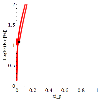
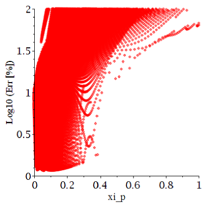
Figure 1: Scatter plots for the error estimation given by Eq. (49) with respect to $\xi_{\rm p}$, obtained by varying the parameters $\mu$ and $\nu$ in Eq. (44). The left panel shows the case with fixed $\mu=1/2$, and the black dot denotes $\mu=1/2$ and $\nu=0$. In the right panel, $\mu$ is also variable. We do not find any point with a small error for $\xi_{\rm p}>0.4$. The empty region around $0<\xi_{\rm p}<0.1$ and $1.5<{\rm Log_{10}(Err)}<2.0$ will be filled by the points if we use a much finer grid for the parameters $\mu$ and $\nu$.

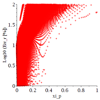
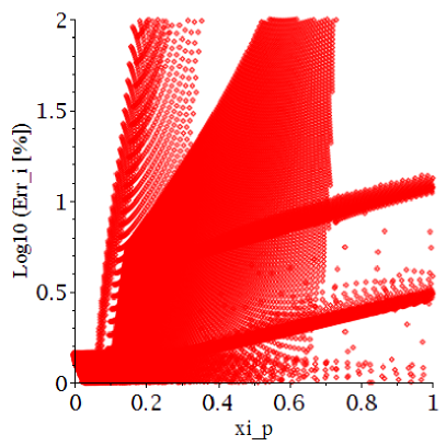
Figure 2: Scatter plots for ${\rm Err}_{\rm r}$ (left) and ${\rm Err}_{\rm i}$ (right) given by Eq. (49) with respect to $\xi_{\rm p}$, obtained by varying the parameters $\mu$ and $\nu$ in Eq. (44).

Varying the parameters $\mu$ and $\nu$, we obtain Fig. 1, which shows the error in the estimation of the QNM frequencies calculated by Eq. (49) with respect to $\xi_{\rm p}$ Figure 2 shows ${\rm Err}_{\rm r}$ (the left panel) and ${\rm Err}_{\rm i}$ (the right panel), respectively. ${\rm Err}$ is dominated by ${\rm Err}_{\rm r}$ for large $\xi_{\rm p}$. We find from Fig. 1 that the region where ${\rm Err}$ given in Eq. (49) is small spreads widely. Although the minimum error of ${\rm Err}\approx 1.2\%$ is obtained for $\mu\approx-0.21$ and $\nu\approx 0.25$ in the analysis, there are many other combinations of $\mu$ and $\nu$ for which ${\rm Err}$ remains small, and the region with small ${\rm Err}$ extends to a range of $0<\xi_{\rm p}<0.4$. Therefore, we should consider that the peak of the potential is located in $0<\xi_{\rm p}<0.4$.

In Refs. Nakamura:2016gri ; Nakano:2016sgf ; Nakamura:2016yjl , we have used the WKB analysis to claim how deeply we can actually inspect the region close to the event horizon of a BH by observing the QNM GWs. Since the GWs cannot be localized and the QNMs are determined not only by the potential at the peak radius but also by the curvature of the potential, what we can claim is that the QNM frequency is determined by the information “around” the peak of the potential. Therefore, it is necessary to properly take into account this fact in the interpretation of the estimated radius obtained in Refs. Nakamura:2016gri ; Nakano:2016sgf ; Nakamura:2016yjl .

The uncertainty in the peak location can be discussed in the following manner. Here, we use $r^{*}_{0}$ instead of $r^{*}_{\rm p}$ because $r^{*}_{0}$ is derived easily in the analytical calculation. Expanding Eq. (45) with respect to $\Delta r^{*}=r^{*}-r^{*}_{0}$ around $r^{*}_{0}$, and using the QNM frequency in the WKB approximation of Eq. (6), we have the radial wavenumber [which corresponds to $W^{1/2}$ in Eq. (59)], as

$$k(r^{*}_{0}+\Delta r^{*}) = \sqrt{\omega_{\rm QNM}^{2}-V}$$ (50)

$$= \sqrt{-\frac{i}{2}\sqrt{-2\left.\frac{d^{2}V}{dr^{*2}}\right|_{r^{*}=r^{*}_{0}}}-\frac{1}{2}\left.\frac{d^{2}V}{dr^{*2}}\right|_{r^{*}=r^{*}_{0}}(\Delta r^{*})^{2}+\cdot\cdot\cdot}\,,$$ (51)

where ($\cdot\cdot\cdot$) denotes the terms of higher order in the WKB approximation or of $O((\Delta r^{*})^{3})$. We note that $d^{2}V/dr^{*2}|_{r^{*}=r^{*}_{0}}=O(\epsilon^{4})$ because $d/dr^{*}=O(\epsilon)\times d/d\xi$ and the $\xi$ dependence of $V$ is as given in Eq. (45). If we expect that the uncertainty of the peak location is given by the inverse of the wavenumber, it may be estimated by the $\Delta r^{*}$ that solves

$$k(r^{*}_{0}+\Delta r^{*})\Delta r^{*}=O(1)\,.$$ (52)

Combining Eqs. (51) and (52), we derive

$$\frac{\left|\Delta r^{*}\right|}{M}=O(\epsilon^{-1})\,,$$ (53)

which is translated into the uncertainty in $\xi_{0}$ as

$$\left|\Delta\xi_{0}\right|=O(1)\,,$$ (54)

by using Eq. (41). This estimate is consistent with the extension of the region where ${\rm Err}$ given in Eq. (49) is small in Fig. 1.

In our previous work Nakamura:2016yjl , we used only one potential which corresponds to $\mu=1/2$ and $\nu=0$ in Eq. (44). The peak location was inside the light ring radius as shown in Eqs. (29) and (37), and we concluded that the QNM GWs were emitted “around” the peak location. However, the meaning of the word “around” was not clear, and Fig. 1 gives a clear explanation of it based on the error estimation of the WKB frequencies compared with the exact QNM frequencies. Using various potentials with the parameters, $\mu$ and $\nu$, even if we change the threshold of the error estimator (49) from a few $\%$ to $10\%$, the extension of the region does not change much from $\xi_{\rm p}\sim 0.4$. Therefore, we conclude that the estimated peak location is restricted to

$$\frac{r_{\rm p}}{M}\lesssim 1+1.8\,(1-q)^{1/2}\,.$$ (55)

The above result confirms that we can see the space-time sufficiently inside the ergoregion ($r_{\rm ergo}=2M$ for the equatorial radius of the ergosurface) and around the inner light ring $r_{\rm lr}/M\approx 1+1.633\,(1-q)^{1/2}$.

4 Discussions

In the modification of the Sasaki–Nakamura equation, we have found that the necessary and sufficient condition for the fast fall-off at $r^{*}\to+\infty$ can be relaxed to the one given by Eq. (28), if we assume that the free functions $g$ and $h$ can be expanded in a power series of $1/r$. When we use $g$ in Eq. (25) which satisfies Eq. (28), the potential is suitable for the WKB analysis of QNMs (see Ref. Nakamura:2016yjl ), but the general expression of the potential is much more complicated than that for $g$ in Eq. (24).

One way to obtain a simple potential will be to keep $\gamma$ constant in the Sasaki–Nakamura transformation. $\gamma$ in Eq. (8) is rewritten as

$$\gamma=A^{2}\left(1-{\frac{\left(\lambda+3\,iK^{\prime}\right)}{\Delta}}\left(\frac{B}{A}\right)^{2}-{\frac{i\left(2\,K+i\Delta^{\prime}\right)}{\Delta}}\left(\frac{B}{A}\right)+\left(\frac{B}{A}\right)^{\prime}\right)\,.$$ (56)

Thus, it is not difficult to find $A$ and $B$ so that $\gamma$ is constant because we may choose $B/A$ which leads $1/A^{2}$ for the expression in the parenthesis of the above equation. The difficult part arises from the condition for $A$ and $B$ that gives a short-ranged potential. To derive such $A$ and $B$ is one of our future studies.

In the study of QNMs in the WKB method, we have evaluated the uncertainty of the peak location of the potential in the extreme Kerr limit. This uncertainty is expressed as Eq. (55), and is consistent with that expected from the equivalence principle.

Here, we should note that the imaginary parts of the QNM frequencies become zero in the extreme Kerr limit, and many overtones ($n\neq 0$) accumulate at one frequency (see, e.g., Fig. 3 in Ref. Cook:2014cta and a recent work Richartz:2015saa ). Therefore, observing QNM GWs in the near-extremal Kerr case will be very different from the other case, and further studies are required to extract the information from extreme Kerr BHs.

Finally, thanks to the recent GW observation, GW150914, we have entered the next stage of using GWs to extract new physics. To test the strong gravitational field around BHs, the QNMs are simple and useful, and the QNM GWs are the target not only for the second-generation GW detectors such as Advanced LIGO (aLIGO) TheLIGOScientific:2014jea , Advanced Virgo (AdV) TheVirgo:2014hva , and KAGRA Somiya:2011np ; Aso:2013eba , but also for space-based GW detectors such as eLISA Seoane:2013qna and DECIGO Seto:2001qf . The enhancement of the signal-to-noise ratio by the third-generation detectors such as the Einstein Telescope (ET) Punturo:2010zz will significantly improve the precision of the test of general relativity.

Appendix A Quasinormal mode in the WKB approximation

We schematically write Eq. (20) as

$$\frac{d^{2}\psi}{dr^{*2}}+W(r^{*})\psi=0\,,$$ (57)

where $W=\omega^{2}-V_{\rm SN}$. In Ref. Schutz:1985zz , the QNM frequencies are discussed as a “second-order turning point” problem in the WKB approximation (see also Ref. BenderOrszag ). We prepare two WKB solutions,

$$\psi_{1}^{\rm WKB}\approx[W(r^{*})]^{-1/4}\exp\left(\pm i\int_{r^{*}_{2}}^{r^{*}}[W(x)]^{1/2}dx\right)\,,$$ (58)

$$\psi_{2}^{\rm WKB}\approx[W(r^{*})]^{-1/4}\exp\left(\pm i\int_{r^{*}}^{r^{*}_{1}}[W(x)]^{1/2}dx\right)\,,$$ (59)

where $r^{*}_{1}$ and $r^{*}_{2}$ are the turning points, and also parabolic cylinder functions for $r^{*}_{1}<r^{*}<r^{*}_{2}$ (see Eq. (5) of Ref. Schutz:1985zz ). The QNM frequencies are derived in the matching condition for the outgoing (from the peak location of the potential) solutions of $\psi_{1}^{\rm WKB}$ and $\psi_{2}^{\rm WKB}$. This means that we choose the signs in Eq. (59) appropriately.

As a usual picture, the peak location is calculated by

$$\frac{dW(r^{*})}{dr^{*}}=0\,,$$ (60)

the solution is denoted by $r^{*}_{0}$, and $r^{*}_{1}<r^{*}_{0}<r^{*}_{2}$ in the case of a real potential. We extend this to a complex potential. Therefore, $r^{*}_{0}$ is in the complex plane.

References

- (1) B. P. Abbott et al. [LIGO Scientific and Virgo Collaborations], Phys. Rev. Lett. 116, 061102 (2016) [arXiv:1602.03837 [gr-qc]].
- (2) B. P. Abbott et al. [LIGO Scientific and Virgo Collaborations], Astrophys. J. 818, L22 (2016) [arXiv:1602.03846 [astro-ph.HE]].
- (3) T. Kinugawa, K. Inayoshi, K. Hotokezaka, D. Nakauchi and T. Nakamura, Mon. Not. Roy. Astron. Soc. 442, 2963 (2014) [arXiv:1402.6672 [astro-ph.HE]].
- (4) T. Kinugawa, A. Miyamoto, N. Kanda and T. Nakamura, Mon. Not. Roy. Astron. Soc. 456, 1093 (2016) [arXiv:1505.06962 [astro-ph.SR]].
- (5) T. Kinugawa, H. Nakano and T. Nakamura, Prog. Theor. Exp. Phys. (2016), 031E01 [arXiv:1601.07217 [astro-ph.HE]].
- (6) T. Hartwig, M. Volonteri, V. Bromm, R. S. Klessen, E. Barausse, M. Magg and A. Stacy, arXiv:1603.05655 [astro-ph.GA].
- (7) B. P. Abbott et al. [LIGO Scientific and Virgo Collaborations], arXiv:1602.03840 [gr-qc].
- (8) J. Healy, C. O. Lousto and Y. Zlochower, Phys. Rev. D 90, 104004 (2014) [arXiv:1406.7295 [gr-qc]].
- (9) A. Ghosh, W. Del Pozzo and P. Ajith, arXiv:1505.05607 [gr-qc].
- (10) E. Berti, J. Cardoso, V. Cardoso and M. Cavaglia, Phys. Rev. D 76, 104044 (2007) [arXiv:0707.1202 [gr-qc]].
- (11) H. Nakano, T. Tanaka and T. Nakamura, Phys. Rev. D 92, 064003 (2015) [arXiv:1506.00560 [astro-ph.HE]].
- (12) R. Konoplya and A. Zhidenko, Phys. Lett. B 756, 350 (2016) [arXiv:1602.04738 [gr-qc]].
- (13) N. Yunes, K. Yagi and F. Pretorius, arXiv:1603.08955 [gr-qc].
- (14) B. P. Abbott et al. [LIGO Scientific and Virgo Collaborations], arXiv:1602.03841 [gr-qc].
- (15) R. P. Kerr, Phys. Rev. Lett. 11, 237 (1963).
- (16) S. A. Teukolsky, Astrophys. J. 185, 635 (1973).
- (17) S. Chandrasekhar and S. L. Detweiler, Proc. Roy. Soc. Lond. A 350, 165 (1976).
- (18) T. Nakamura, H. Nakano and T. Tanaka, Phys. Rev. D 93, 044048 (2016) [arXiv:1601.00356 [astro-ph.HE]].
- (19) H. Nakano, T. Nakamura and T. Tanaka, Prog. Theor. Exp. Phys. (2016) 031E02 [arXiv:1602.02875 [gr-qc]].
- (20) S. L. Detweiler, Proc. Roy. Soc. Lond. A 352, 381 (1977).
- (21) B. Mashhoon, Phys. Rev. D 31, 290 (1985).
- (22) B. F. Schutz and C. M. Will, Astrophys. J. 291, L33 (1985).
- (23) M. Sasaki and T. Nakamura, Phys. Lett. A 89, 68 (1982).
- (24) M. Sasaki and T. Nakamura, Prog. Theor. Phys. 67, 1788 (1982).
- (25) T. Nakamura and M. Sasaki, Phys. Lett. A 89, 185 (1982).
- (26) S. A. Hughes, Phys. Rev. D 62, 044029 (2000) [Phys. Rev. D 67, 089902 (2003)] [gr-qc/0002043].
- (27) T. Nakamura and H. Nakano, Prog. Theor. Exp. Phys. (2016) 041E01 [arXiv:1602.02385 [gr-qc]].
- (28) E. Berti, V. Cardoso and C. M. Will, Phys. Rev. D 73, 064030 (2006) [gr-qc/0512160].
- (29) E. W. Leaver, Proc. Roy. Soc. Lond. A 402, 285 (1985).
- (30) T. Regge and J. A. Wheeler, Phys. Rev. 108, 1063 (1957).
- (31) J. M. Bardeen, W. H. Press and S. A. Teukolsky, Astrophys. J. 178, 347 (1972).
- (32) E. Berti, arXiv:1410.4481 [gr-qc].
- (33) E. Berti, V. Cardoso and A. O. Starinets, Class. Quant. Grav. 26, 163001 (2009) [arXiv:0905.2975 [gr-qc]].
- (34) S. Hod, Phys. Rev. D 78, 084035 (2008) [arXiv:0811.3806 [gr-qc]].
- (35) G. B. Cook and M. Zalutskiy, Phys. Rev. D 90, 124021 (2014) [arXiv:1410.7698 [gr-qc]].
- (36) M. Richartz, Phys. Rev. D 93, 064062 (2016) [arXiv:1509.04260 [gr-qc]].
- (37) J. Aasi et al. [LIGO Scientific Collaboration], Class. Quant. Grav. 32, 074001 (2015) [arXiv:1411.4547 [gr-qc]].
- (38) F. Acernese et al. [VIRGO Collaboration], Class. Quant. Grav. 32, 024001 (2015) [arXiv:1408.3978 [gr-qc]].
- (39) K. Somiya [KAGRA Collaboration], Class. Quant. Grav. 29, 124007 (2012) [arXiv:1111.7185 [gr-qc]].
- (40) Y. Aso et al. [KAGRA Collaboration], Phys. Rev. D 88, 043007 (2013) [arXiv:1306.6747 [gr-qc]].
- (41) P. A. Seoane et al. [eLISA Collaboration], arXiv:1305.5720 [astro-ph.CO].
- (42) N. Seto, S. Kawamura and T. Nakamura, Phys. Rev. Lett. 87, 221103 (2001) [astro-ph/0108011].
- (43) M. Punturo et al., Class. Quant. Grav. 27, 194002 (2010).
- (44) C. M. Bender and S. A. Orszag, Advanced Mathematical Methods for Scientists and Engineers 1, Asymptotic Methods and Perturbation Theory (Springer, New York, 1999).