Abstract

This paper provides some useful tests for fitting a parametric single-index regression model when covariates are measured with error and validation data is available. We propose two tests whose consistency rates do not depend on the dimension of the covariate vector when an adaptive-to-model strategy is applied. One of these tests has a bias term that becomes arbitrarily large with increasing sample size but its asymptotic variance is smaller, and the other is asymptotically unbiased with larger asymptotic variance. Compared with the existing local smoothing tests, the new tests behave like a classical local smoothing test with only one covariate, and still are omnibus against general alternatives. This avoids the difficulty associated with the curse of dimensionality. Further, a systematic study is conducted to give an insight on the effect of the values of the ratio between the sample size and the size of validation data on the asymptotic behavior of these tests. Simulations are conducted to examine the performance in several finite sample scenarios.

Key words: Dimension reduction; error in variable model; model check; adaptive test.

1 Introduction

Consider the nonparametric regression model with measurement error where the response variable $Y$, a $p$-dimensional unobservable predicting covariate $X$ and its observable cohort vector $W$ are related to each other by the relations

$$Y=\mu(X)+\varepsilon,\quad W=X+U.$$ (1.1)

Here $p$ is assumed to be known, and the variables $\varepsilon,\,U,$ and $X$ are assumed to be mutually independent with $E(\varepsilon)=0=E(U)$. Hence $\mu(x)=E(Y|X=x)$ is the usual regression function. This is the so called nonparametric errors in variables (EIVs) regression model. The monographs of Fuller (1987), Cheng and Van Ness (1999), and Carroll, Ruppert, Stefansky and Crainiceanu (2006) contain a vast number of real data examples where this model is naturally applicable.

The problem of interest here is to fit a parametric single-index regression model to the regression function, i.e., for a known real valued link function $g$ we wish to test the hypothesis

$$H_{0}:\,\,\mu(x)=g(\beta^{\top}x),\quad\mbox{for all $x\in{\mathbb{R}}^{p}$ and for some $\beta\in{\mathbb{R}}^{p}$},\,\,\,\mbox{versus}$$

$$H_{1}:\,\,\mbox{$H_{0}$ is not true.}$$

Throughout this paper, $a^{\top}$ denotes transpose of the vector $a\in{\mathbb{R}}^{p}$. The model is called parametric single index although it is also often called generalized linear model. This is because it is in effect slightly different from the generalized linear model that has its special definition in the literature. A motivation for considering the above testing problem is that in practice model checking is necessary to prevent possible wrong conclusions when an improper model is used. Moreover, efficient and accurate inference is possible in a parametric model than in a nonparametric or semiparametric model.

Hart (1997) described numerous tests for lack-of-fit of a parametric regression model in the classical regression set up where $X$ is observable. Since the mid 1990’s, there has been an explosion of activities in this area as is summarized in the recent review by González-Manteiga and Crujeiras (2013).

It is well known that the naive application of the inference procedures valid for the classical regression set up, where one replaces $X$ by $W$, often yields inefficient inference procedures for the EIV models, see, e.g. Fuller (1987) and Carroll et al. (2006). An alternative approach adopted in the literature is that of calibration, where the original regression relationship is transferred to the regression $E(Y|W)$ relationship between the response $Y$ and the cohort $W$. Zhu, Cui and Ng (2004) established a sufficient and necessary condition for the linearity of $E[Y|W]$ with respect to $W$ when $g(\beta^{\top}x)=\alpha+\beta^{\top}x$. A score-type lack-of-fitness test was proposed based on this fact. This testing procedure has been extended to polynomial EIVs models by Cheng and Kukush (2004) and Zhu, Song and Cui (2003) independently, without the normality restriction on the covariates. Hall and Ma (2007) proposed a test based on deconvolution methods assuming that the distribution of the covariate errors is known. Zhu and Cui (2005) proposed a test for fitting a general linear model $\alpha+\beta^{\top}h(x)$, where $h$ is a vector of known functions. Song (2008) proposed a test for fitting $\beta^{\top}h(x)$ to $\mu(x)$, without requiring the knowledge of the density of $X$. He used the deconvolution kernel density estimator. Koul and Song (2009) developed an analog of the minimum distance tests of Koul and Ni (2004) to fit a parametric form to the regression function for the Berkson measurement error models. Koul and Song (2010) developed tests for fitting a parametric function to the nonparametric part in a partial linear regression model under a similar condition. These latter five references assume that density of the measurement error $U$ is known. All of these authors employ the calibrated methodology and test for fitting the parameter form of the regression function $E[Y|W]$ implied by $H_{0}$.

There is no valid test in the literature for fitting a parametric model under general conditions where the distributions of both $X$ and $U$ may not be known. Some of the main reasons for this are the difficulties associated with the estimation of the calibrated regression function and some of the other underlying functions involved in the construction of a test statistic. However, it is possible to circumvent some of these difficulties when there are validation data available. Stute, Xue and Zhu (2007) used validation data and empirical likelihood methodology to develop confidence regions for some underlying parameters. Song (2009) developed a test for general EIVs models with the assistance of validation data without assuming any knowledge of the distributions of $X$ or $U$, under somewhat restrictive conditions on the kernel function and bandwidth. Dai, Sun and Wang (2010) constructed a test with validation data for the same model as in Zhu and Cui (2005). They used specific models and relaxed some conditions in Song (2009). Xu and Zhu (2014) considered a nonparametric test for partial linear EIVs models with validation data. All of these tests are based on local smoothing methodology.

In the classical regression setup, it is known that a common property of lack-of-fit tests for fitting a parametric regression model based on nonparametric smoothing methodology is that the rate of consistency of the test statistics is $1/\sqrt{nh^{p/2}}$. That is, the null distribution of a suitably centered and scaled test statistic multiplied by $\sqrt{nh^{p/2}}$ has a weak limit, and these tests can detect local alternatives distinct from the null only at this rate. When $p$ is even 2 or larger, this rate can be very slow. Consequently, for moderate sample sizes, local smoothing tests cannot maintain the significance level well and have low power even for $p=2$ or $3$. See, e.g., Zheng (1996), Koul and Ni (2002), and several other cited references for this phenomena. It is expected that the same fact will continue to hold for various local smoothing tests in the EIVs setup.

The main goal of the present paper is to propose tests of dimension reduction nature when validation data is available, which do not suffer from the above slow rate of consistency. Specifically, the tests do not suffer severely from the curse of dimensionality and can well maintain the significance level with good power performance for moderate finite sample sizes. Towards this goal we proceed as follows. First, we discuss sufficient dimension reduction (SDR) technique as illustrated in Cook (1998), Li and Yin (2007), and Carroll and Li (1992). The goal is to have a technique such that the dimension of $X$ can be reduced to one-dimensional projection $\beta^{\top}X$ under the null hypothesis, where $\beta$ is just the projection direction in the model (1.1) and to $B^{\top}X$ automatically under the alternative, where $B$ is a $p\times q$ orthonormal matrix with $q\leq p$ to be specified. Second, based on dimension reduction, we can then construct a test with the consistency rate of $1/\sqrt{nh^{1/2}}$ (or $1/(nh^{1/2})$ when a quadratic form is used) when the size $N$ of validation data is proportional to or larger than the sample size $n$. When $N$ is much smaller than $n$, the consistency rate can be slower. Therefore, the third issue is to investigate the relationship between the asymptotic behaviour of the tests and the size of validation data set. In Section 3, a systematic study is performed to analyze the three different scenarios: $N/n\to\lambda$, as $\min(n,N)\to\infty$, where $\lambda=0,\,\infty,$ or $0<\lambda<\infty$. Another interesting issue is raised during the construction procedure. When validation data are used to define the nonparametric kernel estimate of $E(Y|W)$ such that the residuals can be derived, the resulting test would have a bias term going to infinity as $n\to\infty$. It motivates us to consider a bias correction.

To efficiently employ sufficient dimension reduction theory (SDR) of Cook (1998) or CMS of Cook and Li (2002), we consider the alternatives $\tilde{H}_{1}:\mu(x)=G(B^{\top}x),$ for all $x\in{\mathbb{R}}^{p}$, and for some $p\times q$ orthonormal matrix $B$ with an unknown $q\leq p$ and for some real valued function $G$. When there are no measurement errors in covariates, Guo, Wang and Zhu (2015) proposed a dimension-reduction model-adaptive approach to circumvent the dimensionality problem. To implement this methodology one needs to estimate the matrix $B$. There are a number of proposals available in the literature for this purpose. Examples include sliced inverse regression (SIR) of Li (1991), sliced average variance estimation (SAVE) of Cook and Weisberg (1991), contour regression (CR) of Li et al. (2005), directional regression (DR) of Li and Wang (2007), discretization-expectation estimation (DEE) of Zhu et al. (2010a), and the average partial mean estimation (APME) of Zhu et al. (2010b).

In this paper, we construct an adaptive-to-model test in the current set up. The proposed test is based on the Zheng’s test (1996). To this end, we consider a different kind of calibration where instead of conditioning on $W$ we condition on $\beta^{\top}W$ under the null hypothesis and on $B^{\top}W$ under the alternatives, and then constructs a test for this testing problem. Thus, our strategy is sketched as follows: 1). Use the data $(w_{1},y_{1}),\cdots,(w_{n},y_{n})$ to estimate $\beta$ under the null hypothesis and automatically the matrix $B$ by a $q\times q$ orthogonal matrix $C$ under the alternative; 2). Use the validation data to estimate the conditional expectation $E[g(\beta^{\top}X)|\beta^{\top}W]$. 3). Compute the test statistic using these regression function estimates.

As mentioned above, the test statistic is asymptotically biased. It is because of the dependence among the residuals when we use all the validation data to obtain the estimators in Step 2. To reduce the bias, we propose a bias correction method to construct another test. In the simulation studies, we will compare their performance.

The paper is organized as follows: Section 2 contains a brief description of the test statistic construction. Since the estimation the matrix $B$ plays a key role in having the dimension reduction property of the test, we review a widely used dimension reduction method in this section. The needed assumptions are also stated in this section. The asymptotic properties of the test statistic under the null and alternative hypotheses are described in Section 3. Particularly, a systematic study is conducted on the asymptotic behaviors of the tests under the three scenarios where the ratio $N/n$ of the validation data $N$ and the sample size $n$ is small, moderate and large. Section 4 presents the simulation results. The proofs are postponed to Appendix.

Before closing this section, we describe some notation used in the sequel. The sample is denoted by $\{(y_{i},w_{i}),i=1,\cdots,n\}$ and the validation data is dented by $\{(\tilde{w}_{s},\tilde{x}_{s}),s=1,\cdots,N\}$. The two data sets are assumed to independent of each other. Further, in various expressions below, $i$ and $j$ often represent the indices of primary data, while $s$ and $t$ those of validation data. Throughout this paper, $\to_{p}$ denotes the convergence in probability and ”$\to_{D}$” stands for the convergence in distribution. All limits are taken as $n\wedge N\to\infty$, unless specified otherwise. The normal distribution with mean $a$ and variance $b$ is denoted by $N(a,b)$.

2 Methodology development

2.1 Test construction: a dimension-reduction adaptive-to-model strategy

In this subsection, we describe the details of test statistics construction. It consists of three components as follows.
1). Model adaptation. To proceed further, let $r(w,\beta)=E[g(\beta^{\top}X)|W=w]$, $w\in{\mathbb{R}}^{p}$, denote the new regression function under the null hypothesis. In order to avoid the above mentioned high dimensionality problem of nonparametric estimators of $r(\cdot,\cdot)$ due to the dimension of $W$, we adopt the following dimension reduction adaptive-to-model strategy (DREAM). Recall that $W=X+U$. Note that under $H_{0}$, the regression function $g(\beta^{\top}X)$ depends on $X$ only through the linear combination $\beta^{\top}X$. It is then natural to consider the situation where the calibrated regression function $E(Y|W)$ depends on $W$ only through a linear combination of the components of $W$, i.e., when $E(Y|W)=E[g(\beta^{\top}X)|W]=E[g(\beta^{\top}X)|\beta^{\top}W]:=r(\beta^{\top}W,\beta)$. Similarly, under the alternative, we assume that $E(Y|W)=E(Y|B^{\top}W)=E(G(B^{\top}X)|B^{\top}W)$. Thus the transferred hypotheses become as follows:

$${\cal H}_{0}:P\{E(Y|W)=r(\beta^{\top}W,\beta)\}=1,\quad\text{ for some $\beta\in{\mathbb{R}}^{p}$},$$ (2.1)

versus the transferred alternative hypothesis:

$${\cal H}_{1}:P\{E(Y|W)=E(Y|B^{\top}W)\not=r(\beta^{\top}W,\beta)\}=1,\quad\text{for all $\beta\in{\mathbb{R}}^{p}$ }.$$ (2.2)

Generally the two hypotheses $H_{0}$ and ${\cal H}_{0}$ are not exactly equivalent. But, as in Song (2008), when the family densities $f_{\beta^{\top}U}(\beta^{\top}w-\cdot)$ is a complete family over the parameter $\beta^{\top}w\in{\mathbb{R}}$, the equivalence can hold.

2). Test statistic construction. Let $e=Y-r(\beta^{\top}W,\beta)$. To unify the null and alternatives, let $B=\beta c$ under ${\cal H}_{0}$ where $c$ is a constant, hence $E[e|\beta^{\top}W]=E[e|B^{\top}W]=0$. Moreover, following Zheng (1996),

$$E[eE[e|\beta^{\top}W]f(\beta^{\top}W)]=E[E^{2}(e|\beta^{\top}W)f(\beta^{\top}W)]=E[E^{2}(e|B^{\top}W)f(B^{\top}W)]=0,$$

and under ${\cal H}_{1}$, $E[E^{2}(e|B^{\top}W)f(B^{\top}W)]>0$. To obtain residuals for the construction of the test statistics, we assume the availability of validation data $(w_{s},x_{s}),s=1,\cdots,N$, which is used to estimate the function $r$. Note that $r$ is an unknown function of $\beta^{\top}W$. In order to construct an estimator $r(\beta^{\top}W,\beta)$, let $M(\cdot)$ be a kernel function, $v_{N}$ be a bandwidth sequence, and set $M_{v_{N}}(\cdot)=v_{N}^{-1}M(\cdot/v_{N})$. Then an estimator of $r(\beta^{\top}W,\beta)$ is

$$\hat{r}(\hat{\beta}^{\top}w,\hat{\beta})=\frac{\sum_{s=1}^{N}M_{v_{N}}(\hat{\beta}^{\top}w-\hat{\beta}^{\top}\tilde{w}_{s})g(\hat{\beta}^{\top}\tilde{x}_{s})}{\sum_{s=1}^{N}M_{v_{N}}(\hat{\beta}^{\top}w-\hat{\beta}^{\top}\tilde{w}_{s})},$$ (2.3)

where $\hat{\beta}$ is a consistent estimate of $\beta$ based on primary data. Define the residuals

$$e_{i}=y_{i}-r(\beta^{\top}w_{i},\beta),\quad\hat{e}_{i}=y_{i}-\hat{r}(\hat{\beta}^{\top}w_{i},\hat{\beta}),\quad i=1,\cdots,n.$$ (2.4)

To estimate the conditional expectation of the error $e$, given $B^{\top}W$, we also need an estimator $\hat{B}(\hat{q})$ of $B$ that is consistent to $\beta/\|\beta\|$ under the null, and to $B$ under the alternative. This model adaptation property of $\hat{B}(\hat{q})$ can enable the test statistic to adapt to model and then to alleviate the curse of dimensionality. This estimator will be specified later. For the moment assume the existence of such an estimator.

To proceed further, let $K$ be another kernel function and $h\equiv h_{n}$ another bandwidth. Then an estimator of the product $E[e|B^{\top}W]f(B^{\top}W)$ at $\hat{B}^{\top}w_{i}$ is given by

$$\hat{E}[e_{i}|\hat{B}(\hat{q})^{\top}w_{i}]\hat{f}(\hat{B}(\hat{q})^{\top}w_{i}) = \frac{1}{n-1}\sum_{j\neq i}^{n}K_{h}(\hat{B}(\hat{q})^{\top}w_{j}-\hat{B}(\hat{q})^{\top}w_{i})\hat{e}_{j}.$$

The analog of the Zheng’s test statistic in the current set up is based on an estimator of $E[eE[e|W]f(W)]$, given by

$$\tilde{V}_{n}=\frac{1}{n(n-1)}\sum_{i=1}^{n}\sum_{j\neq i}^{n}\hat{e}_{i}K_{h}(\hat{B}(\hat{q})^{\top}(w_{i}-w_{j}))\hat{e}_{j}.$$ (2.5)

3). Bias correction. From the technical details in Appendix, we can see that the test statistic in (2.5) has non-negligible asymptotic bias and thus its limiting null distribution has a mean tending to infinity unless $n/(Nh^{1/2})\to 0$, which makes the bias term vanish. The main reason is the dependence between the residuals $\hat{e}_{i}$ and $\hat{e}_{j}$ for $i\not=j$ when all validation data are used to estimate the function $r$. There are two ways to correct for this bias. One is to center the test statistic at a suitable estimator of this bias. This is a traditional method, and has been used. Alternately, we propose a block-wise estimation approach to asymptotically eliminate the bias as follows. Assume $N$ is a positive even integer. We halve the whole validation data set, use the two halves to construct two estimators of the regression function $r$, which results in the two sets of residuals as follows. Let

$$\hat{r}_{(1)}(\hat{\beta}^{\top}w,\hat{\beta})=\frac{\sum_{s=1}^{N/2}M_{v_{N}}(\hat{\beta}^{\top}w-\hat{\beta}^{\top}\tilde{w}_{s})g(\hat{\beta}^{\top}\tilde{x}_{s})}{\sum_{s=1}^{N/2}M_{v_{N}}(\hat{\beta}^{\top}w-\hat{\beta}^{\top}\tilde{w}_{s})},$$

$$\hat{r}_{(2)}(\hat{\beta}^{\top}w,\hat{\beta})=\frac{\sum_{s=N/2+1}^{N}M_{v_{N}}(\hat{\beta}^{\top}w-\hat{\beta}^{\top}\tilde{w}_{s})g(\hat{\beta}^{\top}\tilde{x}_{s})}{\sum_{s=N/2+1}^{N}M_{v_{N}}(\hat{\beta}^{\top}w-\hat{\beta}^{\top}\tilde{w}_{s})},$$

$$\hat{e}_{i(1)}:=y_{i}-\hat{r}_{(1)}(\hat{\beta}^{\top}w_{i},\hat{\beta}),\quad\hat{e}_{i(2)}=y_{i}-\hat{r}_{(2)}(\hat{\beta}^{\top}w_{i},\hat{\beta}),\quad i=1,\cdots,n.$$

Use these residuals to define the test statistic

$$V_{n}=\frac{1}{n(n-1)}\sum_{i=1}^{n}\sum_{j\neq i}^{n}\hat{e}_{i(1)}K_{h}(\hat{B}(\hat{q})^{\top}w_{i}-\hat{B}(\hat{q})^{\top}w_{j})\hat{e}_{j(2)}$$ (2.7)

to perform the test. We shall prove that the asymptotic bias of $V_{n}$ vanishes, but its asymptotic variance gets larger than that of $\tilde{V}_{n}$. Note that $\tilde{V}_{n}$ and $V_{n}$ are non-standardized, the standardizing constants will be specified in Section 3. Here, we mention a significant feature of both of these statistics, which is that their asymptotic behavior is like that of a test statistic with one-dimensional covariate $X$, i.e., their consistency rate is $1/\sqrt{nh^{1/2}}$, which in turn greatly alleviates the dimensionality issue.

From the above construction, it is obvious that estimating adaptively the matrix $B$ under the null and alternative hypothesis plays a crucial role for dimension reduction. The next subsection is devoted to this issue.

2.2 Estimation of B and $\beta$

To achieve the adaptation property of the estimators of $B$ and $\beta$ mentioned above, the key is to derive an estimator of $B$ up to an $q\times q$ orthonormal matrix $C$ without depending on the assumed models under the null and alternative hypotheses. With measurement errors, Carroll and Li (1992) extended sliced inverse regression (SIR, Li 1991) to errors-in-variables regression models. Lue (2004) extended the principal Hessian directions (pHd, Li 1992) method to the surrogate problem. Li and Yin (2007) established a general invariance law between the surrogate and the original dimension reduction spaces when $X$ and $U$ are jointly multivariate normal. If $X$ or $U$ is not normally distributed, they suggested an approximation based on the results of Hall and Li (1993). See also Zhang, Zhu and Zhu (2014).

As the discretization-expectation estimation method (DEE) of Zhu et al.  (2010a) is simple to implement without selecting the number of slices, we adopt it to errors-in-variables models when SIR is used. Write $S_{Y|X}$ as the central subspace that is the intersection of all column spaces spanned by the columns of $B$ that makes $Y$ conditionally independent of $X$, given $B^{\top}X$, i.e., $Y\bot\!\!\!\bot X|B^{\top}X$. This means that identifying $S_{Y|X}$ is equivalent to identifying a base matrix $\tilde{B}$ that is equal to $BC^{\top}$ for a $q\times q$ orthogonal matrix $C$. Note that the function $G$ is unknown in the alternative. We can rewrite $G(B^{\top}X)$ as $\tilde{G}(\tilde{B}^{\top}X)$. In other words, identifying $\tilde{B}$ is enough for model identification. Without notational confusion, we write $\tilde{B}=B$ throughout the rest of this paper.

To extend the DEE method to the setting with measurement errors, we first give a very brief review. Assume that $\mbox{Cov}(X)$ is the identity matrix. As is known, SIR is fully dependent on the reverse regression function $E(X|Y)$ such that we can consider the eigen-decomposition of its covariance matrix $\mbox{Cov}(E(X|Y))$. The eigen vectors associated with nonzero eigen values of this matrix form the base matrix $B$. SIR-based DEE uses the matrix $\Lambda=E\{\mbox{Cov}(E(X|\tilde{Y}(T)))\}$ as the target matrix, where $\tilde{Y}(t)=I(Y\leq t)$, $t\in{\mathbb{R}}$ and $T$ is an independent copy of $Y$. Because the measurement error $U$ is independent of $Y$, and thus, when $X$ is replaced by $W$, at the population level, nothing is changed about eigen-decomposition and eigen vectors. We use surrogate predictors $\mbox{Cov}(X,W)\Sigma_{W}^{-1}W$, which forms the least squares prediction of X when W is given. Carroll and Li (1992) pointed out that sliced inverse regression (SIR) with the surrogate predictors can produce consistent estimators of $S_{Y|X}$. In other words, all steps of estimation are exactly the same as those in the without measurement errors set up. The reader can refer to Zhu et al.  (2010a) for more details.

When we use data to construct an estimate $\Lambda_{n}$ of $\Lambda$, we can then obtain an estimate $\hat{B}(\hat{q})$ of $B$, which consists of the $\hat{q}$ eigenvectors of $\Lambda_{n}$ with non-zero eigenvalues, where $\hat{q}$ is defined as follows, using the BIC type criterion proposed by Zhu et al.  (2006). Let $\hat{\lambda}_{1}\geq\hat{\lambda}_{2}\geq\cdots\geq\hat{\lambda}_{p}$ be the eigen values of the matrix $\Lambda_{n}$ in descending order. An estimate $\hat{q}$ of $q$ is given by

$$\hat{q}=\arg\max_{l=1,\cdots,p}\left\{\frac{n}{2}\times\frac{\sum_{i=1}^{l}\{\log(\hat{\lambda}_{i}+1)-\hat{\lambda}_{i}\}}{\sum_{i=1}^{p}\{\log(\hat{\lambda}_{i}+1)-\hat{\lambda}_{i}\}}-2\times D_{n}\times\frac{l(l+1)}{2p}\right\},$$ (2.8)

where $D_{n}$ is a sequence of constants not depending on the data. Here we take $D_{n}=n^{1/2}$.

The following consistency results can be obtained from Zhu et al.  (2010a).

Proposition 2.1

Suppose the assumptions in Zhu et al.  (2010a) hold and $N/n\to\lambda$. Then the following hold.
(1). Under $H_{0}$, $P(\hat{q}=1)\to 1$, and $B$ is a vector proportional to $\beta$. Moreover,

$$\hat{B}(\hat{q})-B = O_{p}(1/\sqrt{n}),\quad 0<\lambda\leq\infty,$$

$$= O_{p}(1/\sqrt{N}),\hskip 22.76228pt\lambda=0.$$

(2). Under $H_{1}$, $P(\hat{q}=q)\to 1$, $B$ is a $p\times q$ orthonormal matrix and $\hat{B}(\hat{q})$ satisfies (2.1).

There are various estimators of $\beta$ for EIVs models available in the literature. Here we shall focus on the estimators proposed by Lee and Sepanski (1995) for linear and nonlinear EIVs regression models. Their estimator under the null hypothesis is

$$\hat{\beta}=\arg\min_{\beta}({\mathbf{Y}}-{\mathbf{D}}({\mathbf{D}}_{v}^{\top}{\mathbf{D}}_{v})^{-1}{\mathbf{D}}_{v}g({\mbox{\boldmath$X$}}_{v}\beta))^{\top}(Y-{\mathbf{D}}({\mathbf{D}}_{v}^{\top}{\mathbf{D}}_{v})^{-1}{\mathbf{D}}_{v}g({\mbox{\boldmath$X$}}_{v}\beta))$$

where ${\mathbf{X}}_{v}$ is the $N\times p$ matrix whose sth row is $\tilde{x}_{s}^{T},s=1,\cdots,N$, ${\mathbf{Y}}$ is a $n\times 1$ vector, and $g({\mbox{\boldmath$X$}}_{v}\beta)$ represents $N\times 1$ vector $[g(\beta^{\top}\tilde{x}_{1}),\cdots,g(\beta^{\top}\tilde{x}_{N})]^{\top}$. The matrices ${\mathbf{D}}$ and ${\mathbf{D}}_{v}$ are design matrices according to $g(\cdot)$. More precisely, ${\mathbf{D}}$ is the $n\times k$ matrix whose $i$-th row denoted by $\bar{w}^{{}^{\prime}}_{i}$, is a vector consisting of polynomials of $w_{i}$, while ${\mathbf{D}}_{v}$ is the corresponding matrix of validation data, whose $s$-th row $\bar{w}_{s}$ is a vector consisting of polynomials of $\tilde{w}_{s}$. For linear model, $\bar{w}_{i}=w_{i}$ and $\bar{w}_{s}=\tilde{w}_{s}$. For nonlinear model, we let $\bar{w}_{i}$($\bar{w}_{s}$) be the vector consisting of a constant and the first two order polynomials of $w_{i}$($\tilde{w}_{s}$). Lee and Sepanski (1995) assume that $\lim\sqrt{n/N}$ exists. They show that if this limit is non-negative and finite then $\hat{\beta}$ is root-$n$ consistent for $\beta$, and if $\lim\sqrt{n/N}=\infty$, then $\hat{\beta}$ is a root-$N$ consistent for $\beta$. More precisely, we have the following proposition.

Proposition 2.2

Suppose the assumptions for Proposition 2.2 in Lee and Sepanski (1995) hold.
(1). Suppose in addition $H_{0}$ holds and $N/n\to\lambda$. Then for $0<\lambda\leq\infty$, $\sqrt{n}(\hat{\beta}-\beta)=O_{p}(1)$, while for $\lambda=0$, $\sqrt{N}(\hat{\beta}-\beta)=O_{p}(1)$.
(2). In addition, suppose the following sequence of local alternatives holds, where $C_{n}\to 0$.

$$H_{1n}:\mu(x)=g(\beta^{\top}x)+C_{n}G(x).$$

Then

$$\hat{\beta}-\beta_{0} = C_{n}\left\{E[g^{\prime}(\beta^{\top}X)X\bar{W}^{\top}]E^{-1}[\bar{W}\bar{W}^{\top}]E[g^{\prime}(\beta^{\top}X)\bar{W}X^{\top}]\right\}^{-1}$$

$$\hskip 14.22636pt\times E[g^{\prime}(\beta^{\top}X)X\bar{W}^{\top}]E^{-1}[\bar{W}\bar{W}^{\top}]E[\bar{W}G(X)](1+o_{p}(1))$$

$$+O_{p}(1/\sqrt{n})+O_{p}(1/\sqrt{N}).$$

where $\bar{W}$ is a vector consist of polynomials of $W$ and $g^{\prime}(t)$ is the derivative of $g(t)$ with respect to $t$.

3 Asymptotic distributions

3.1 Limiting null distribution

In this section, we will establish the asymptotic null distribution of the proposed test statistics $\tilde{V}_{n}$ in (2.5) and $V_{n}$ in (2.7). Define

$$Z=B^{\top}W,\quad\sigma^{2}(Z)=E[e^{2}|Z],\quad\Delta(Z)=E[G(B^{\top}X)|Z],$$ (3.1)

$$\eta=g(\beta^{\top}X)-r(\beta^{\top}W,\beta),\quad\xi^{2}(Z)=E[\eta^{2}|Z],$$

where $e$ is defined in (2.4). Write $Z$ as $\tilde{Z}$, when $W$ is replaced by validation data $\tilde{W}$.

To proceed further we now state the assumptions needed here.

Assumptions:
(f). The support $\mathcal{C}$ of $Z$ is a compact subset of the support of $\tilde{Z}$ and bounded away from the boundary of the support of $\tilde{Z}$. The density $f$ of $Z$ has bounded partial derivatives up to order $\ell\geq 1$ and satisfies

$$0<\inf_{z\in\mathcal{C}}f(z)\leq\sup_{z\in\mathcal{C}}f(z)<\infty.$$

(g). $g(\beta^{\top}x)$ is a measurable function of $x$ for each $\beta$ and is differentiable in $\beta$ up to order $\ell+1$, and $E\big{\|}\frac{\partial g(\beta_{0}^{\top}X)}{\partial\beta}\big{\|}^{2}<\infty$. (r). The function $r(\beta^{\top}w,\beta)$ has bounded partial derivatives with respect to $\beta^{T}w$ up to order $\ell+1$, and $E[r^{2}(\beta^{\top}W,\beta)]<\infty$, $\beta\in{\mathbb{R}}^{p}$. (G). $E[\Delta^{2}(Z)]<\infty$, $E[(G(B^{\top}X)-\Delta(Z))^{4}]<\infty$, and $\Delta(z)$ has bounded partial derivatives up to order $\ell$. (W). $\max_{1\leq k\leq p}E[W^{2}_{(k)}|Z]<\infty$, $W_{(k)}$ represents the $k$-th coordinate of $W$, $k=1,\cdots,p$. (e). $E[(\sigma^{2}(Z))^{2}]<\infty$, $E[(\xi^{2}(Z))^{2}]<\infty$, and $\sigma^{2}(z)$ and $\xi^{2}(z)$ are uniformly continuous functions. (K). $K$ is a spherically symmetric and continuous kernel function with bounded support and of order $\ell$, having all derivatives bounded. (M). $M$ is a symmetric and continuous kernel function with bounded support and of order $\ell$, having all derivatives bounded. (h1). $h\to 0$, $v_{N}\to 0$, $v_{N}/h\to 0$. (h2). $h\to 0$, $v_{N}\to 0$, $h^{4}/v_{N}^{5}\to 0$. (h3). $nh^{2}\to\infty$, $Nv_{N}^{2}\to\infty$, $nv_{N}^{2\ell}\to 0$ and $nhv_{N}/N\to 0$. (h4). $nh^{5/2}\to\infty$, $Nv_{N}^{2}\to\infty$, $nv_{N}^{2\ell}\to 0$ and $nhv_{N}/N\to 0$. (h5). $nh\to\infty$, $Nh^{2}\to\infty$, $Nv_{N}^{1/2}/(nh^{1/2})\to 0$ and $Nv_{N}^{1/2+2\ell}\to 0$. (h6). $nh^{q}\to\infty$, $Nv_{N}\to\infty$.

The positive integer $\ell$ in all of the above assumptions is the same as in the assumption (f). For the consistency of $\hat{\beta}$ and $\hat{B}(\hat{q})$, some additional conditions are also needed. The reader can refer to Lee and Sepanski (1995) and Zhu et al.  (2010a) for more details.

Remark 3.1

Conditions (g), (r), (W), (e) are very common for the asymptotic normality of the proposed test statistics. The lower bound assumption on $f$ is typically designed for the nonparametric estimation of the corresponding regression function $r(\beta^{\top}W,\beta)$ and the conditional mean $E[e|Z]$. This is a commonly used condition. In assumption (h6), $nh^{q}\to\infty$ is to ensure the consistency in quadratic mean of kernel density estimator under some global alternative. If $v_{N}/h\to 0$, some convolution of kernel functions can be approximated by kernel function. If $N/n\to\infty$ or a finite constant, this condition is easily satisfied. We choose $v_{N}=O((N/2)^{-2/5})$ in the simulation studies later. But when $N/n\to 0$, the condition is changed to $h/v_{N}\to 0$.

To proceed further, we need some more notation as follows:

$$z_{i}=B^{\top}w_{i},\quad g_{i}=g(\beta^{\top}x_{i}),\quad r_{i}=r(\beta^{\top}w_{i},\beta),\quad\eta_{i}=g_{i}-r_{i}.$$ (3.2)

Write $\tilde{z}_{s}$, $\tilde{g}_{s}$, $\tilde{r}_{s}$ and $\tilde{\eta}_{s}$ for the entities in (3.2) when $w_{i}$ is replaced by validation data $\tilde{w}_{s}$ in there. When $\beta$ and $B$ are respectively replaced by their estimators $\hat{\beta}$ and $\hat{B}(\hat{q})$ in the above definitions, write the respective $\hat{z}_{i}$, $\hat{g}_{i}$, $\hat{r}_{i}$ and $\hat{\eta}_{i}$ for $z_{i}$, $g_{i}$, $r_{i}$ and $\eta_{i}$, and similarly write the respective $\hat{\tilde{z}}_{s}$, $\hat{\tilde{g}}_{i}$, $\hat{\tilde{r}}_{i}$ and $\hat{\tilde{\eta}}_{i}$ for $\tilde{z}_{i}$, $\tilde{g}_{i}$, $\tilde{r}_{i}$ and $\tilde{\eta}_{i}$.

To state the next theorem we need to define

$$\mu=K(0)E[\xi^{2}(z)]/(Nh),\qquad\tau_{1}=2\int K^{2}(u)du\int(\sigma^{2}(z))^{2}f^{2}(z)dz,$$ (3.3)

$$\tau_{2}=\int K^{2}(u)du\int\sigma^{2}(z)\xi^{2}(z)f^{2}(z)dz,\quad\tau_{3}=2\int K^{2}(u)du\int(\xi^{2}(z))^{2}f^{2}(z)dz.$$

where $\sigma^{2}(\cdot)$ and $\xi^{2}(\cdot)$ are defined in (3.1) and $f$ is the density of $Z=B^{\top}W$. Consistent estimates of $\Sigma_{i},i=1,2,3$ under $H_{0}$ are given by

$$\hat{\tau}_{1}=\frac{2}{n(n-1)}\sum_{i=1}^{n}\sum_{j\neq i}^{n}\frac{1}{h^{\hat{q}}}K^{2}(\frac{\hat{z}_{i}-\hat{z}_{j}}{h})\hat{e}_{i}^{2}\hat{e}_{j}^{2},\quad\hat{\tau}_{2}=\frac{1}{nN}\sum_{i=1}^{n}\sum_{s=1}^{N}\frac{1}{h^{\hat{q}}}K^{2}(\frac{\hat{z}_{i}-\hat{\tilde{z}}_{s}}{h})\hat{e}_{i}^{2}\hat{\tilde{\eta}}_{s}^{2}$$ (3.4)

$$\hat{\tau}_{3}=\frac{2}{N(N-1)}\sum_{s=1}^{N}\sum_{s^{{}^{\prime}}\neq s}^{N}\frac{1}{h^{\hat{q}}}K^{2}(\frac{\hat{\tilde{z}}_{s}-\hat{\tilde{z}}_{s^{{}^{\prime}}}}{h})\hat{\tilde{\eta}}_{s}^{2}\hat{\tilde{\eta}}_{s{{}^{\prime}}}^{2}.$$

We are now ready to state

Theorem 3.1

Suppose $H_{0}$ and the conditions (f), (g), (r), (W), (e), (K), (M), (h1) and (h3) hold, and that $N/n\to\lambda$, $0<\lambda\leq\infty$. Then $nh^{1/2}\big{(}\tilde{V}_{n}-\mu\big{)}\to_{D}N(0,\tilde{\tau}),$ where

$$\tilde{\tau} = \tau_{1}+\frac{2}{\lambda}\tau_{2}+\frac{1}{\lambda^{2}}\tau_{3},\quad 0<\lambda<\infty,$$

$$= \tau_{1},\hskip 101.17755pt\lambda=\infty.$$

Here, consistent estimators of $\mu$ and $\tau$ under $H_{0}$ are given by

$$\hat{\mu}=\frac{1}{N^{2}h}K(0)\sum_{s=1}^{N}\hat{\tilde{\eta}}_{s}^{2},\qquad\hat{\tilde{\tau}}=\hat{\tau}_{1}+\frac{2}{\lambda}\hat{\tau}_{2}+\frac{1}{\lambda^{2}}\hat{\tau}_{3},\quad 0<\lambda<\infty,$$

with $\hat{\tau}_{i}$’s as in (3.4). The $\tilde{V}_{n}$ test rejects $H_{0}$ whenever $\tilde{V}_{n}>\hat{\tilde{\tau}}^{1/2}(nh^{1/2})^{-1}z_{\alpha}+\hat{\mu}$, where $z_{\alpha}$ is the upper $100(1-\alpha)\%$ quantile of the standard normal distribution.

The above theorem shows that the asymptotic variance of $\tilde{V}_{n}$ consists of the three parts when $0<\lambda<\infty$. The part $\tau_{1}$ reflects the variation in the regression model, $\tau_{3}$ is the variation caused by the measurement error while the part $\tau_{2}$ is the intersection of the variation due to the regression model and measurement error.

The next result gives the asymptotic null distribution of the $V_{n}$ statistic of (2.7). As can be seen from this result, $V_{n}$ does not have any asymptotic bias.

Theorem 3.2

Under the conditions of Theorem 3.1, $nh^{1/2}V_{n}\to_{D}N(0,\tau),$ where

$$\tau = \tau_{1}+\frac{4}{\lambda}\tau_{2}+\frac{2}{\lambda^{2}}\tau_{3},\quad 0<\lambda<\infty,$$

$$= \tau_{1},\hskip 101.17755pt\lambda=\infty,$$

where $\tau_{i}$, $i=1,2,3,$ are as in (3.3).

To studentize $V_{n}$, we use the following consistent estimate of $\tau$ in the case $0<\lambda<\infty$.

$$\hat{\tau}= \frac{2}{n(n-1)}\sum_{i=1}^{n}\sum_{j\neq i}^{n}\frac{1}{h^{\hat{q}}}K^{2}(\frac{\hat{z}_{i}-\hat{z}_{j}}{h})\hat{e}_{i(1)}^{2}\hat{e}_{j(2)}^{2}+\frac{4}{\lambda nN}\sum_{i=1}^{n}\sum_{s=N/2+1}^{N}\frac{1}{h^{\hat{q}}}K^{2}(\frac{\hat{z}_{i}-\hat{\tilde{z}}_{s}}{h})\hat{e}_{i(1)}^{2}\hat{\tilde{\eta}}_{s}^{2}$$

$$+\frac{4}{\lambda nN}\sum_{i=1}^{n}\sum_{t=1}^{N/2}\frac{1}{h^{\hat{q}}}K^{2}(\frac{\hat{z}_{i}-\hat{\tilde{z}}_{t}}{h})\hat{e}_{i(2)}^{2}\hat{\tilde{\eta}}_{t}^{2}+\frac{16}{\lambda^{2}N^{2}}\sum_{t=1}^{N/2}\sum_{s=N/2+1}^{N}\frac{1}{h^{\hat{q}}}K^{2}(\frac{\hat{\tilde{z}}_{s}-\hat{\tilde{z}}_{t}}{h})\hat{\tilde{\eta}}_{s}^{2}\hat{\tilde{\eta}}_{t}^{2},$$

where $s$ and $t$ are indices of the two sets of validation data respectively, $\hat{\eta}_{t}$ or $\hat{\eta}_{s}$ is estimated by the other half of validation data. That is, $\hat{\tilde{\eta}}_{t}=g(\hat{\beta}^{\top}\tilde{x}_{t})-\hat{r}_{(2)}(\hat{\beta}^{\top}\tilde{w}_{t},\hat{\beta})$, $t=1,\cdots,N/2$ and $\hat{\tilde{\eta}}_{s}=g(\hat{\beta}^{\top}\tilde{x}_{s})-\hat{r}_{(1)}(\hat{\beta}^{\top}\tilde{w}_{s},\hat{\beta})$, $s=N/2+1,\cdots,N,$ where $\hat{r}_{(1)}$ and $\hat{r}_{(2)}$ are defined in (2.1). The standardized test statistic is

$$T_{n} = \hat{\tau}^{-1/2}nh^{1/2}V_{n},\quad 0<\lambda<\infty,$$

$$= \hat{\tau}_{1}^{-1/2}nh^{1/2}V_{n},\hskip 22.76228pt\lambda=\infty,$$

where $\hat{\tau}_{1}$ is as in (3.4). According to the Slusky theorem, $T_{n}$ is asymptotically standard normal. At the significance level $\alpha$, the null hypothesis is rejected when $T_{n}>z_{\alpha}$. For large $\lambda$, the terms about $\tau_{2}$ and $\tau_{3}$ vanish in the asymptotic variance, and thus, the estimated variance $\hat{\tau}$ is replaced by $\hat{\tau}_{1}$.

Remark 3.2

A significant feature of this test is that we only need to use the standardizing sequence $nh^{1/2}$, which is the same as the one used in the classical local smoothing tests when $X$ is one-dimensional. This shows that the test statistic has a much faster convergence rate to its limit compared to some of the classical tests that have the rate of order $nh^{p/2}$. This greatly assists in maintaining the significance level of this test in finite samples when its asymptotic null distribution is used to determine the critical values for its implementation.

When $N/n\to\lambda=0$, the standardizing constant will be different because of the plug-in estimate $\hat{r}(\cdot)$ of the function $r(\cdot)$, as is evidenced by the following theorem.

Theorem 3.3

Suppose $H_{0}$ and the above conditions (f), (g), (r), (W), (e), (K), (M), (h2), (h5) hold and that $N/n\to 0$. Then $Nv_{N}^{1/2}\{\tilde{V}_{n}-\nu\}\to_{D}N(0,\tilde{\tau}),$   $Nv_{N}^{1/2}V_{n}\to_{D}N(0,\tau),$ where $\nu=\|\beta\|(v_{N}N)^{-1}\int M^{2}(u)du\,E[\xi^{2}(Z)],$   $\tau:=2\tilde{\tau},$ and

$$\tilde{\tau}=2\|\beta\|\int\Big{(}\int M(u)M(u+v)du\Big{)}^{2}dv\int(\xi^{2}(z))^{2}f^{2}(z)dz.$$

3.2 Asymptotic Power

In this section, we assume $N/n\to\lambda$, $\lambda$ a positive constant and investigate the asymptotic properties of the test statistic $V_{n}$ under global and local alternatives. This is because the asymptotic properties can be much more easily derived than those for $\tilde{V}_{n}$. Consider a sequence of alternatives

$$H_{1n}:\mu(x)=g(\beta^{\top}x)+C_{n}G(B^{\top}x),\quad x\in{\mathbb{R}}^{p},$$ (3.5)

where $G(\cdot)$ satisfies $E(G^{2}(B^{\top}X))<\infty$ and $\beta$ is a column of $B$. When $C_{n}$ is a fixed constant, the alternative is a global alternative and when $C_{n}=n^{-1/2}h^{-1/4}$ tends to zero, $H_{1n}$ specify the local alternatives of interest here. Note that the asymptotic properties of the estimates $\hat{B}(\hat{q})$ and $\hat{\beta}$ will affect the behavior of the test statistic $V_{n}$. The asymptotic results of $\hat{\beta}$ have been illustrated in Proposition  2.2. Thus, we discuss the result about the consistency of $\hat{q}$ here. Under the local alternatives, it is no longer consistent for the dimension $q$.

Theorem 3.4

Suppose the conditions in Zhu et. al (2010a) hold. Under $H_{1n}$ of (3.5) with $C_{n}=n^{-1/2}h^{-1/4}\to 0$, $P(\hat{q}=1)\to 1$.

However, this inconsistency does not hurt the power performance of the test. We will see below in a finite sample simulation study that the test can be much more powerful than the classical local smoothing tests in the literature.

Theorem 3.5

Under the alternatives of (3.5), the following results are hold:
(i)Suppose (f), (g), (r), (G), (W), (e), (K), (M), (h1) and (h6) hold. Under the global alternative with fixed $C_{n}$,

$$V_{n}/\hat{\tau}\to V>0.$$ (3.6)

(ii) Suppose (f), (g), (r), (G), (W), (e), (K), (M), (h1) and (h4) hold. Then, under the local alternatives $H_{1n}$ with $C_{n}=n^{-1/2}h^{-1/4}$, $nh^{1/2}V_{n}\to_{D}N(\Delta,\tau)$, where $\tau$ is given in Theorem 3.2 and $\Delta=E\left[\{\Delta(Z)-E[g{{}^{\prime}}(\beta_{0}^{\top}X)X^{\top}|Z]H(\beta_{0})\}^{2}f(Z)\right].$

Remark 3.3

The result (3.6) implies the consistency of the $T_{n}$ test gainst the class of the above fixed alternative. It also implies that under the global alternatives, the test statistic can diverge to infinity at a much faster rate than the existing local smoothing tests in the literature can achieve such as Zheng’s test (1996), which has the consistency rate of the order $1/(nh^{p/2})$. The test can also detect the local alternatives distinct from the null at the rate of order $1/\sqrt{nh^{1/2}}$ while the classical ones can only detect those alternatives converging to the null at the rate of order $1/\sqrt{nh^{p/2}}$.

4 Numerical studies

This section presents four simulation studies to examine the performance of the proposed test ($T_{n}$). To compare with existing tests, we consider Zheng’s (1996) test ($T_{n}^{Zh}$) adapted to the errors-in-variables settings and Song’s (2009) test ($T^{S}_{n}$) as the competitors. The adapted Zheng’s test is the same as our test except that $B^{\top}W$ is replaced by the original $W$. This is a typical local smoothing test. Song’s test is a score type test and is designed for EIVs models with validation data. Consider the linear regression models under the null hypothesis. In the simulation study 1 below, the matrix $B$ is equal to $\beta$ and thus, the model is a parametric single index. The dimension of $X$ is respectively $p=2$ and $8$. Note that our test fully uses the information under the null hypothesis that only relates to a single index $\beta$. In addition, we run simulation studies of the test $\tilde{T}_{n}$ based on the statistic $\tilde{V}_{n}$ of Theorem 3.1 when $0<\lambda<\infty$, and illustrate its weakness. The purpose of Study 2 is to confirm that the proposed test $T_{n}$ is not a directional test by assuming $B=(\beta_{1},\beta_{2})$ with $q=2$ under the alternative hypothesis. Study 3 is designed to examine the finite sample performance when $N<n$ and $N>n$. Study 4 considers four nonlinear models. All simulations are based on 2000 replications.

Recall that the tests $T_{n}$ and $T_{n}^{Zh}$ are based on the estimates of the quantities that are zero under the null and positive under the alternative. Because of the asymptotic normality, the rejection regions of $\tilde{V}_{n}$, $T_{n}$ and $T_{n}^{Zh}$ are one-sided: $\{\tilde{V}_{n}>\hat{\tilde{\tau}}^{1/2}(nh^{1/2})^{-1}1.65+\hat{\mu}\}$, $\{T_{n}>1.65\}$ and $\{T_{n}^{Zh}>1.65\}$ at the $0.05$ level of significance. The reported size and power are computed by $\#\{T_{n}>1.65\}/2000$. For $T^{S}_{n}$, the rejection region is two sided and the reported size and power are computed by $\#\{|T^{S}_{n}|>1.96\}/2000$. Throughout the simulation studies, $X$ is taken to be multivariate normal with mean zero and covariance matrices $\Sigma_{1}=I_{p\times p}$ and $\Sigma_{2}=(0.3^{|i-j|})_{p\times p}$. The regression model error $\varepsilon$ follows standard normal distribution, while the measurement error $U\sim N(0,0.5)$. The kernel function is $K(u)=\frac{15}{16}(1-u^{2})^{2}I(|u|\leq 1)$ which is a second-order symmetric kernel and $M(u)=K(u)$.

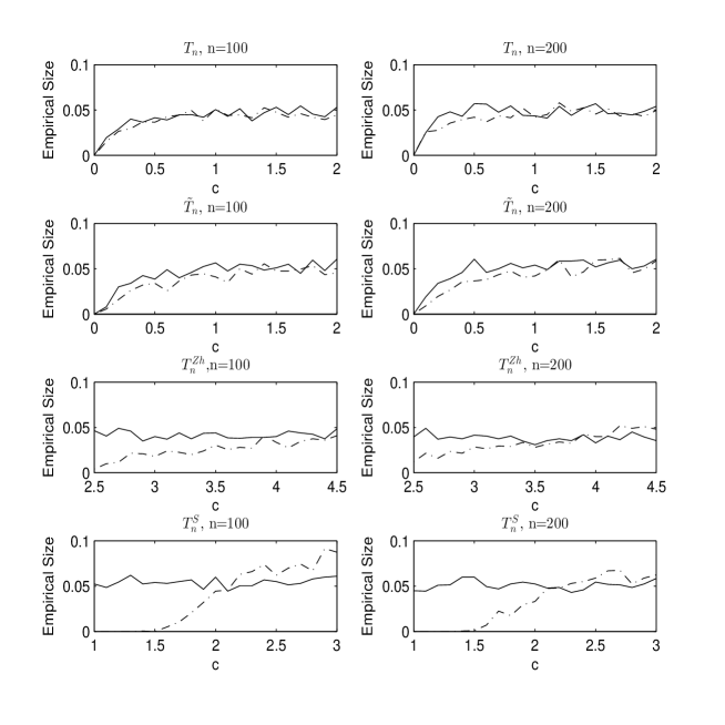
Figure 1: Plots for the empirical size curve against different values of $c$ in the bandwidths $h=cn^{-1/(4+q)}$, $v_{N}=c(N/2)^{-2/5}$. For model $Y=\beta^{\top}X+\epsilon$, the solid lines are with $p=2$, $q=1$ and the dash-dotted lines are with $p=8$, $q=1$.

Bandwidth selection.   As the tests involve bandwidth selection in the kernel estimation, we run a simulation to empirically select the bandwidths for the three tests in the comparison. Because the significance level maintainance is important, we then select bandwidths such that the tests can have empirical sizes close to the significance level and retain the use under other models. To this end, we use a simple model to select them and to check whether they can be used in general. In our test, there are two bandwidths. As is well known, the optimal bandwidth in hypothesis testing is still an outstanding problem, but the optimal rate of the bandwidth in kernel estimation is $n^{-1/(4+q)}$ where $n$ is the sample size. We then adopt its rate with a search for the constant $c_{1}$ in $h=c_{1}n^{-1/(4+\hat{q})}$. Similarly, for the kernel estimator of the function $r(\beta^{\top}W,\beta)$, we choose the window width $v_{N}=c_{2}(N/2)^{-2/5}$, because we halved the validation data set of size $N$. For $\tilde{T}_{n}$, $v_{N}$ is $c_{2}N^{-2/5}$. To select proper bandwidths, we tried different bandwidths to investigate their impact on the empirical size. To reduce the computational burden, we consider $c_{1}=c_{2}=c$ to see whether such selections can offer bandwidths for general use. The selection is based on hypothetical models as the primary target is to maintain the significance level. Thus, we compute the empirical size at every equal gird point $c=(i-1)/10$ for $i=1,\cdots 21$. In Figure 1, we report the empirical sizes associated with different bandwidths when the regression model is $\mu(x)=\beta^{\top}x$ and $p=2,8$, $n=100,200$, $N=4\times n$, and the covariance matrix of $X$ is $\Sigma_{1}$. We can see that the test is not very sensitive to the bandwidth and a value of $c=1.6$ may be a good choice for both $T_{n}$ and $\tilde{T}_{n}$. For the adapted Zheng’s test, there are also two bandwidths to be selected. As the optimal rate for the kernel estimation is $h=c_{1}n^{-1/(4+p)}$, we then also consider $c_{1}=c_{2}=c$. We found that to maintain the significance level, the bandwidths must be with larger $c$. The initial selection provides us an idea to choose a good bandwidth within the equal grid points as $c=2.5+(i-1)/10$ for $i=1,\cdots 21$. The results are also reported in Figure 1. As for Song’s score test, only one bandwidth is required. We also found a larger bandwidth is required. Set the bandwidth as $v_{N}=cN^{-1/(4+p)}$ and search for the proper $c$ within the equal grid points as $c=1+(i-1)/10$ for $i=1,\cdots 21$. The reported curves are in Figure 1.

Figure  1. about here

We can see that the empirical sizes of $T_{n}$ are not sensitively affected by the bandwidths selected. The curves of empirical size under $p=2$ and $p=8$ are almost coincident. While the empirical size of $\tilde{T}_{n}$ is slightly effected by dimensionality, but it is still more robust than that of $T_{n}^{Zh}$ and $T_{n}^{S}$. A value of $c=1.6$ is worthy of recommendation for both, $T_{n}$ and $\tilde{T}_{n}$. However, the empirical sizes of $T_{n}^{Zh}$ and $T_{n}^{S}$ associated with the bandwidths are not as robust as that of $T_{n}$. The empirical sizes show the efficient bandwidth changes as $p$ increase. When $p$ is small, a small $h$ can keep the theoretical size. As $p$ increase, a larger $h$ is necessary. This phenomenon is particularly serious for $T_{n}^{Zh}$. For the bandwidths of $T_{n}^{Zh}$, $c=3.9$ is appropriate. Finally, $c=2.2$ seems to be proper for $T_{n}^{S}$.

Study 1. The data are generated from the following model:

$$H_{11}:\,\,\mu(x)=\beta^{\top}x+a\,(\beta^{\top}x)^{2},$$

$$H_{12}:\,\,\mu(x)=\beta^{\top}x+a\,\exp(-(\beta^{\top}x)^{2}/2),$$

$$H_{13}:\,\,\mu(x)=\beta^{\top}x+2a\cos(0.6\pi\beta^{\top}x).$$

The case of $a=0$ corresponds to the null hypothesis and $a\not=0$ to the alternatives. In other words, both the hypothetical and alternative models have a single index $B=c\beta$. Models under $H_{11}$ and $H_{12}$ represent low frequency alternatives while $H_{13}$ is an example of high frequency alternative. In $H_{11}$ and $H_{12}$, the alternative parts $(\beta^{\top}x)^{2}$ and $\exp(-(\beta^{\top}x)^{2}/2$ always exist for any nonzero $a$. While for $H_{13}$, the alternative part $\cos(0.6\pi\beta^{\top}x)$ appears and disappears periodically for $a\neq 0$, which makes the bandwidth selection process even more challenging. Because a large bandwidth selected to maintain significance level may make the test obtuse to high frequency alternatives. The dimension $p$ equals $2$ and $8$ such that we can check the impact from the dimensionality. Let $\beta=(1,1,\cdots,1)^{\top}/\sqrt{p}$. The number of validation data is $N=4n$. The simulation results are presented in Tables 1, 2 and 3.

Tables 1-3 about here

From these tables we see that when $p=2$, $T^{S}_{n}$ performs very well. This is expected when the dimension is low or moderate, because the consistency rate of this test is $1/\sqrt{n}$. Also, when $p$ is small, $T_{n}^{Zh}$ is comparable to $T_{n}$ as both are local smoothing tests. When the dimension increases, $T_{n}^{Zh}$ and $T^{S}_{n}$ are however severely impacted by the dimensionality. The test $T_{n}^{Zh}$ behaves much worse. Especially, when $p=8$, it breaks down for $n=100$ and regains its power as $n$ increase. The test $T^{S}_{n}$ is also affected by the dimensionality because the residuals contain nonparametric estimation by local smoothing technique. Its powers decrease both for small and large sample size. On the other hand, the dimension-reduction adaptive-to-model test $T_{n}$ does not suffer from the curse of dimensionality in the limited simulation studies presented here. When $p$ is large, $T_{n}$ performs better than $T^{S}_{n}$. The finite sample power of the $T^{S}_{n}$ test is poor against the alternatives $H_{13}$ for both the cases $p=2$ and $p=8$. This may be due to the fact that $T^{S}_{n}$ is a directional test. We illustrate this problem in the next study.

The comparison between $T_{n}$ and $\tilde{T}_{n}$ is another purpose of this study. We find that the empirical power of $\tilde{T}_{n}$ is slightly higher than that of $T_{n}$, but the size of $\tilde{T}_{n}$ also tends to be slightly larger, even when $n=200$ and $p=2$. Although $\tilde{T}_{n}$ has bias, but each residual in $\tilde{T}_{n}$ is estimated by all validation data which is more precise with smaller variance than that of $T_{n}$ derived by half validation dat. We can then conclude, based on this limited simulation, the test $\tilde{T}_{n}$ is slightly more liberal than the bias-corrected test $T_{n}$, but also slightly more powerful. These two tests are competitive. Therefore, in the following simulation studies, we only report the results about $T_{n}$ to save space.

Study 2. In this study, we aim to design a simulation study to check that the dimension-reduction model-adaptive test $T_{n}$ is not a directional test, while Song’s test $T^{S}_{n}$ is. The data are generated from the following model:

$$H_{14}:\,\,\mu(x)=\beta_{1}^{\top}x+a(\beta_{2}^{\top}x)^{2},\qquad H_{15}:\,\,\mu(x)=2\beta_{1}^{\top}x+a(2\beta_{2}^{\top}x)^{3}.$$

Here also, $a=0$ corresponds to the null hypothesis and $a\neq 0$ to the alternatives. The matrix $B=(\beta_{1},\beta_{2})$ and then the structural dimension $q$ under the alternative is $2$. Let $p=4$, $\beta_{1}=(1,1,0,0)^{\top}/2$ and $\beta_{2}=(0,0,1,1)^{\top}/2$. The number of validation data is $N=4\times n$. The simulation results are presented in Table 4. From these results, we first observe that $T^{S}_{n}$ has good performance under $H_{14}$, which coincides with that in Study 1. However, the poor performance under $H_{15}$ shows that $T^{S}_{n}$ is a directional test as this alternative cannot be detected by it at all. At population level, we can see that the conditional expectation of the residual is equal to zero under this alternative. In this case, $T_{n}$ still works well. This lends support to the claim that $T_{n}$ is an omnibus test.

Tables 4 about here

Study 3. In this study, we aim to explore the impact of the estimation of $r(\cdot)$ on the performance of the proposed tests. Small $\lambda=\lim(N/n)$ means that there are not many validation data available and large $\lambda$ means the estimator $\hat{r}(\cdot)$ is very close to the true function $r(\cdot)$. For this purpose, consider $N/n=0.1,0.5,4,8$. We only choose these ratios because if $\lambda$ is either too small or too large, we need to have too large sample size or too large size of validation data. These are practically not possible. From Theorem 3.3, we know that when $\lambda$ is small, we can have a test with simpler limiting variance. Write the related test as $T_{n}^{(1)}$. From Theorem 3.2, $\lambda=\infty$ case, we can also have a test for large $N/n$. Write it as $T_{n}^{(2)}$. To examine whether these two variants of the test $T_{n}$ work or not, we generate data from the model $H_{11}$ in Study 1. When the size of validation data is such that $N/n=0.1,0.5$, $T_{n}^{(1)}$ is used, and when $N/n=4,8$, $T_{n}^{(2)}$ is applied. As $T_{n}^{(1)}$ is a test with very different convergence rate, we then also need to choose bandwidths suitable for it. Similarly as the above, we also search for the bandwidths at the rates $v_{N}=c_{1}(N/2)^{-1/3}$ and $h=c_{2}n^{-1/(2+\hat{q})}$. Let $c_{1}=c_{2}=c$. We found that $c=2$ is a good choice. For $T_{n}^{(2)}$, only the asymptotic variance changes, we then still use the same bandwidths as before. When $\lambda=0.1,0.5$, we then use larger sample size of validation data $N=100,200$, otherwise, $N$ is too small to make the tests well performed. The simulation results are presented in Table 5.

Table 5 about here

From Table 5, we have the following two observations. First, for $\lambda=0.1$, $T_{n}$ is more conservative with lower power than $T_{n}^{(1)}$. This seems to say, $T_{n}$ is less sensitive to the alternative model than $T_{n}^{(1)}$. This phenomenon would come from the improper selection of bandwidths for $T_{n}$ because Conditions (h1) and (h2) assure that the consistency of $T_{n}$ and $T_{n}^{(1)}$ require different ratios of $h$ and $v_{N}$. Thus, when $N/n$ is very small, $T_{n}^{(1)}$ seems to be a better choice than $T_{n}$. But when $\lambda$ is closed to 1, $T_{n}^{(1)}$ cannot maintain the significance level well. Secondly, $T_{n}^{(2)}$ has very slightly higher empirical size and power than $T_{n}$. Overall, the performances of $T_{n}^{(2)}$ is very similar to that of $T_{n}$. Therefore, when the size of validation data $N$ is reasonably large, and the ratio $N/n$ is large, $T_{n}^{(2)}$ would be applicable. Also, from the simulations we see that although $T_{n}^{(1)}$ can be used, it does not maintain the finite sample significance level as well as the $T_{n}$ test does. Thus, when the ratio $N/n$ is not too small, we recommend the test $T_{n}$, rather than $T_{n}^{(1)}$, for practical use.

Study 4. In this study, a nonlinear single-index null model is considered. We try four alternatives with different structural dimension as follows:

$$H_{16}:\,\,Y=(\beta^{\top}X)^{3}+a|\beta^{\top}X|+\epsilon$$

$$H_{17}:\,\,Y=(\beta^{\top}X)^{3}+aX_{3}^{2}+\epsilon$$

$$H_{18}:\,\,Y=(\beta^{\top}X)^{3}+a(X_{2}/4+|X_{3}^{2}|+\cos(\pi X4))+\epsilon$$

$$H_{19}:\,\,Y=(\beta^{\top}X)^{3}+a(X_{2}/2+X_{3}^{2}+\cos(\pi X_{4})+X_{5}\exp(X_{6}/2)+X_{8}X_{7})+\epsilon$$

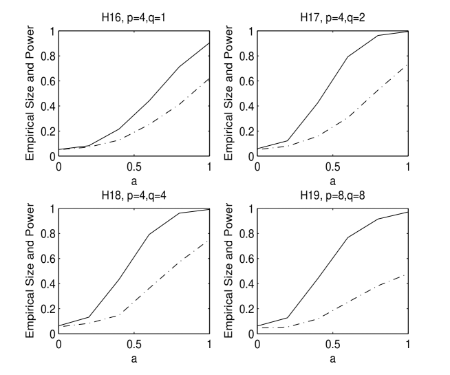
Figure 2: Plots of power curves over $a$ under $H{16}-H{19}$ in Study 4. The solid lines are for $T_{n}$ and the dash-dotted lines are for $T_{n}^{Zh}$.

Let $p=4$ for $H_{16}$, $H_{17}$, $H_{18}$ and $p=8$ for $H_{19}$. $\beta=[1,0,\cdots,0]^{\top}$. $\Sigma=\Sigma_{1}$, $\sigma_{u}=0.5$. $a$ is designed to be $0,0.2,0.4,0.6,0.8,1.0$. In these cases, $q$ is always 1 for the null but different for alternatives. For $H_{16}$, $q=1$ for any nonzero $a$. The structure dimension under $H_{17}$ is 2, and under $H_{18},$ $p=q=4$. For $H_{19}$, $p=q=8$. The test $T_{n}$ uses the same bandwidths as chosen for linear model above. For $T_{n}^{Zh}$, we adjust bandwidths to keep its performance. Set $c=2.7$ for $H_{16}$, $H_{17}$, $H_{18}$ and $c=3$ for $H_{19}$. The results are presented in Figure 2.

Figure 2. about here

We have the following observations. First, the model-adaptive method $T_{n}$ has greater empirical power than $T_{n}^{Zh}$ for all chosen alternatives. Under $H_{18}$ and $H_{19}$, though convergence rate of the two teats are same, $T_{n}$ is still more powerful than $T_{n}^{Zh}$. Because $T_{n}$ is constructed by $nh^{1/2}V_{n}/\sqrt{\Sigma}=h^{(1-q/2)}\times nh^{q/2}V_{n}/\sqrt{\Sigma}$. Secondly, the power of $T_{n}^{Zh}$ decreases quickly as $p$ increases while that of $T_{n}$ does not.

5 Appendix. Proofs

This section is organized as follows. In Section 5.1, Proposition 2.2 is proved. The proof of Theorem 3.4 appears in Section  5.2. Based on the asymptotic behavior of $\hat{\beta}$ and $\hat{B}$ under the local alternatives, the proof of Theorem 3.5 is included in Section 5.3. As Theorem 3.2 is a special case of Theorem 3.5 when $C_{n}=0$, its proof is omitted. In Section 5.4, we only sketch the proof of Theorem 3.1 as it is similar to that of Theorem 3.5. Section 5.5 shows a sketch of the proof for Theorem 3.3.

5.1 Proof of Proposition  2.2

The claim (1) has been proved in Lee and Sepanski (1995). We now prove the claim (2). Recall some notation: ${\mathbf{X}}$ is $n\times p$ matrix whose $i$th row is $x_{i}^{\top},i=1,\cdots,n$, ${\mathbf{X}}_{v}$ is the $N\times p$ matrix whose $s$th row is $\tilde{x}_{s}^{\top},s=1,\cdots,N$, and ${\mathbf{Y}}$ is a $n\times 1$ vector, while $g({\mathbf{X}}_{v}\beta)$ represents the $N\times 1$ vector and equals to $[g(\beta^{\top}\tilde{x}_{1}),\cdots,g(\beta^{\top}\tilde{x}_{N})]^{\top}$. The matrix ${\mathbf{D}}$ is the $n\times k$ matrix whose $i$-th row $\bar{w}^{\top}_{i}$ is a $1\times k$ vector consist of polynomials of $w_{i}$. The matrix ${\mathbf{D}}_{v}$ is the corresponding matrix of validation data, whose $s$-th row $\bar{w}^{\top}_{s}$ is a vector consist of polynomials of $\tilde{w}_{s}$. For linear model, $\bar{w}_{i}=w_{i}$ and $\bar{w}_{s}=\tilde{w}_{s}$. For nonlinear model, we let $\bar{w}_{i}$ be a vector consisting of a constant and the first two order polynomials of $w_{i}$.

Let

$$Q_{n}(\beta)=\frac{1}{n}\Big{(}{\mathbf{Y}}-{\mathbf{D}}({\mathbf{D}}_{v}^{\top}{\mathbf{D}}_{v})^{-1}{\mathbf{D}}_{v}^{\top}g({\mathbf{X}}_{v}\beta)\Big{)}^{\top}\Big{(}{\mathbf{Y}}-{\mathbf{D}}({\mathbf{D}}_{v}^{\top}{\mathbf{D}}_{v})^{-1}{\mathbf{D}}_{v}^{\top}g({\mathbf{X}}_{v}\beta)\Big{)}.$$

The estimator $\hat{\beta}$ satisfies the first order condition: $\partial Q_{n}(\hat{\beta})/\partial\beta=0$. By Taylor expansion and the mean value theorem:

$$\Big{[}\frac{\partial g^{\top}({\mathbf{X}}_{v}\beta_{0})}{\partial\beta}{\mathbf{D}}_{v}\Big{]}({\mathbf{D}}_{v}^{\top}{\mathbf{D}}_{v})^{-1}{\mathbf{D}}^{\top}({\mathbf{Y}}-{\mathbf{D}}({\mathbf{D}}_{v}^{\top}{\mathbf{D}}_{v})^{-1}{\mathbf{D}}_{v}^{\top}g({\mathbf{X}}_{v}\beta_{0}))$$

$$= \Big{\{}\Big{[}\frac{\partial^{2}g^{\top}({\mathbf{X}}_{v}\bar{\beta})}{\partial\beta\partial\beta^{\top}}{\mathbf{D}}_{v}\Big{]}({\mathbf{D}}_{v}^{\top}{\mathbf{D}}_{v})^{-1}{\mathbf{D}}^{\top}({\mathbf{Y}}-{\mathbf{D}}({\mathbf{D}}_{v}^{\top}{\mathbf{D}}_{v})^{-1}{\mathbf{D}}_{v}^{\top}g({\mathbf{X}}_{v}\bar{\beta}))$$

$$-\Big{[}\frac{\partial g^{\top}({\mathbf{X}}_{v}\bar{\beta})}{\partial\beta}{\mathbf{D}}_{v}\Big{]}({\mathbf{D}}_{v}^{\top}{\mathbf{D}}_{v})^{-1}({\mathbf{D}}^{\top}{\mathbf{D}})({\mathbf{D}}_{v}^{\top}{\mathbf{D}}_{v})^{-1}[\frac{\partial g^{\top}({\mathbf{X}}_{v}\bar{\beta})}{\partial\beta}{\mathbf{D}}_{v}]\Big{\}}(\beta_{0}-\hat{\beta})$$

where $\bar{\beta}$ is a vector satisfying $\|\bar{\beta}-\beta\|\leq\|\hat{\beta}-\beta_{0}\|$, and

$$[\frac{\partial^{2}g^{\top}({\mathbf{X}}_{v}\bar{\beta})}{\partial\beta\partial\beta^{\top}}{\mathbf{D}}_{v}]=[\frac{\partial^{2}g^{\top}({\mathbf{X}}_{v}\bar{\beta})}{\partial\beta\partial\beta_{1}}{\mathbf{D}}_{v},\cdots,\frac{\partial^{2}g^{\top}({\mathbf{X}}_{v}\bar{\beta})}{\partial\beta\partial\beta_{p}}{\mathbf{D}}_{v}].$$

Let $g^{\prime}$, $g^{\prime\prime}$ denote the first and second derivatives of $g$, respectively. By the LLNs,

$$\frac{1}{N}\frac{\partial g^{\top}({\mathbf{X}}_{v}\beta)}{\partial\beta}{\mathbf{D}}_{v}=\frac{1}{N}\sum_{s=1}^{N}g{{}^{\prime}}(\beta^{\top}\tilde{x}_{s})\tilde{x}_{s}\bar{w}_{s}^{\top}\to_{p}E[g{{}^{\prime}}(\beta^{\top}X)X\bar{W}^{\top}],$$

$$\frac{1}{N}\frac{\partial^{2}g^{\top}({\mathbf{X}}_{v}\bar{\beta})}{\partial\beta\partial\beta_{l}}{\mathbf{D}}_{v}\to_{p}E[g{{}^{\prime\prime}}(\beta^{\top}X)X_{(l)}X\bar{W}^{\top}],$$

and

$$\frac{1}{n}{\mathbf{D}}^{\top}(Y-{\mathbf{D}}({\mathbf{D}}_{v}^{\top}{\mathbf{D}}_{v})^{-1}{\mathbf{D}}_{v}^{\top}g({\mathbf{X}}_{v}\bar{\beta}))$$

$$= C_{n}E[\bar{W}G(X)]+(E[\bar{W}g(\beta_{0}^{\top}X)]-E(\bar{W}\bar{W}^{\top})\gamma_{0})+o_{p}(1)$$

$$= o_{p}(1),$$

where $\gamma_{0}=E^{-1}(\bar{W}\bar{W}^{\top})E[\bar{W}g(\beta_{0}^{\top}X)]$. Hence

$$\hat{\beta}-\beta_{0} = \bigg{\{}[\frac{\partial^{2}g^{\top}({\mathbf{X}}_{v}\bar{\beta})}{\partial\beta\partial\beta^{\top}}{\mathbf{D}}_{v}]({\mathbf{D}}_{v}^{\top}{\mathbf{D}}_{v})^{-1}{\mathbf{D}}^{\top}({\mathbf{Y}}-{\mathbf{D}}({\mathbf{D}}_{v}^{\top}{\mathbf{D}}_{v})^{-1}{\mathbf{D}}_{v}^{\top}g({\mathbf{X}}_{v}\bar{\beta}))$$

$$-[\frac{\partial g^{\top}({\mathbf{X}}_{v}\bar{\beta})}{\partial\beta}{\mathbf{D}}_{v}]({\mathbf{D}}_{v}^{\top}{\mathbf{D}}_{v})^{-1}({\mathbf{D}}^{\top}{\mathbf{D}})({\mathbf{D}}_{v}^{\top}{\mathbf{D}}_{v})^{-1}[\frac{\partial g^{\top}({\mathbf{X}}_{v}\bar{\beta})}{\partial\beta}{\mathbf{D}}_{v}]\bigg{\}}^{-1}$$

$$\times[\frac{\partial g^{\top}({\mathbf{X}}_{v}\beta_{0})}{\partial\beta}{\mathbf{D}}_{v}]({\mathbf{D}}_{v}^{\top}{\mathbf{D}}_{v})^{-1}{\mathbf{D}}^{\top}({\mathbf{Y}}-{\mathbf{D}}({\mathbf{D}}_{v}^{\top}{\mathbf{D}}_{v})^{-1}{\mathbf{D}}_{v}^{\top}g({\mathbf{X}}_{v}\beta_{0}))$$

$$= \left\{E[g{{}^{\prime}}(\beta^{\top}X)X\bar{W}^{\top}]E^{-1}[\bar{W}\bar{W}^{\top}]E[g{{}^{\prime}}(\beta^{\top}X)\bar{W}X^{\top}]+O_{p}(C_{n})\right\}^{-1}$$

$$\times\left\{E[g{{}^{\prime}}(\beta^{\top}X)X\bar{W}^{\top}]E^{-1}[\bar{W}\bar{W}^{\top}]\right\}\frac{1}{n}{\mathbf{D}}^{\top}({\mathbf{Y}}-{\mathbf{D}}({\mathbf{D}}_{v}^{\top}{\mathbf{D}}_{v})^{-1}{\mathbf{D}}_{v}^{\top}g({\mathbf{X}}_{v}\beta)).$$

On the other hand,

$$\frac{1}{n}{\mathbf{D}}^{\top}({\mathbf{Y}}-{\mathbf{D}}({\mathbf{D}}_{v}^{\top}{\mathbf{D}}_{v})^{-1}{\mathbf{D}}_{v}^{\top}g({\mathbf{X}}_{v}\beta))$$

$$= \frac{1}{n}{\mathbf{D}}^{\top}C_{n}G({\mathbf{X}})+\frac{1}{n}{\mathbf{D}}^{\top}(g({\mathbf{X}}\beta)+\varepsilon-{\mathbf{D}}({\mathbf{D}}_{v}^{\top}{\mathbf{D}}_{v})^{-1}{\mathbf{D}}_{v}^{\top}g({\mathbf{X}}_{v}\beta))$$

$$= \frac{C_{n}}{n}\sum_{i=1}^{n}\tilde{w}_{i}G(x_{i})+\frac{1}{n}{\mathbf{D}}^{\top}(g({\mathbf{X}}\beta)+\varepsilon-{\mathbf{D}}E^{-1}[\bar{W}\bar{W}^{\top}]E[\bar{W}^{\top}g(\beta^{\top}X)])$$

$$-\left(\frac{1}{n}{\mathbf{D}}^{\top}{\mathbf{D}}\right)\left[\frac{1}{N}{\mathbf{D}}_{v}^{\top}{\mathbf{D}}_{v}\right]^{-1}\frac{1}{N}({\mathbf{D}}_{v}^{\top}g({\mathbf{X}}_{v}\beta)-{\mathbf{D}}_{v}^{\top}{\mathbf{D}}_{v}E^{-1}[\bar{W}^{\top}\bar{W}]E[\bar{W}^{\top}g(\beta^{\top}X)])$$

$$= C_{n}E[\bar{W}G(x)]+O_{p}(1/\sqrt{n})+O_{p}(1/\sqrt{N}).$$

This completes the proof of part (2) of Proposition 2.2.

5.2 Proof of Theorem 3.4

Denote $\zeta=\mbox{Cov}(X,W)\Sigma_{W}^{-1}W$. In the discretization step, we construct new samples $(\zeta_{i},I(y_{i}\leq y_{j}))$. For each $y_{j}$, we estimate $\Lambda(y_{j})$ which spans $S_{I(Y\leq y_{j})|\zeta}$ by using SIR and denote the estimate by $\Lambda_{n}(y_{j})$. In the expectation step, we estimate $\Lambda=E[\Lambda(t)]$, which spans $S_{Y|\zeta}$, by $\Lambda_{n,n}=n^{-1}\sum_{j=1}^{n}\Lambda_{n}(y_{j})$. Let $\lambda_{1}>\lambda_{2}>\cdots>\lambda_{q}>\lambda_{q+1}=0=\cdots=\lambda_{p}$ be the descending sequence of eigenvalues of the matrix $\Lambda$ and $\hat{\lambda}_{1}\geq\hat{\lambda}_{2}\geq\cdots\geq\hat{\lambda}_{p}$ be the descending sequence of eigenvalues of the matrix $\Lambda_{n,n}$. Recall the $D_{n}$ in $\hat{q}$ of (2.8) was selected as $\sqrt{n}$. Define the objective function in (2.8) as

$$G(l)=\frac{n}{2}\times\frac{\sum_{i=1}^{l}\{\log(\hat{\lambda}_{i}+1)-\hat{\lambda}_{i}\}}{\sum_{i=1}^{p}\{\log(\hat{\lambda}_{i}+1)-\hat{\lambda}_{i}\}}-2\times n^{1/2}\times\frac{l(l+1)}{2p}.$$

Now we prove that for any $l>1$, $P(G(1)>G(l))\to 1$, i.e., $P(\hat{q}=1)\to 1$.

$$G(1)-G(l)=n^{1/2}\times\frac{l(l+1)-2}{p}-\frac{n}{2}\times\frac{\sum_{i=2}^{l}\{\log(\hat{\lambda}_{i}+1)-\hat{\lambda}_{i}\}}{\sum_{i=1}^{p}\{\log(\hat{\lambda}_{i}+1)-\hat{\lambda}_{i}\}}$$

If $\Lambda_{n,n}-\Lambda=O_{p}(C_{n})$, then $\hat{\lambda}_{i}-\lambda_{i}=O_{p}(C_{n})$. By the second order Taylor Expansion, we have $\log(\hat{\lambda}_{i}+1)-\hat{\lambda}_{i}=-\hat{\lambda}^{2}_{i}+o_{p}(\hat{\lambda}^{2}_{i})$. Thus, $\sum_{i=2}^{l}\{\log(\hat{\lambda}_{i}+1)-\hat{\lambda}_{i}\}=O_{p}(C^{2}_{n})$ and $\sum_{i=1}^{p}\{\log(\hat{\lambda}_{i}+1)-\hat{\lambda}_{i}\}$ converge to a negative constant in probability. Since $nC_{n}^{2}/n^{1/2}\to 0$ and $l(l+1)>2$, $P(G(1)>G(l))\to 1$.

Now we check the condition of $\Lambda_{n,n}-\Lambda=O_{p}(C_{n})$. First, we investigate the convergence rate of $\Lambda_{n}(t)-\Lambda(t)$ for any fixed $t$. We have

$$\Lambda(t)=\Sigma_{\zeta}^{-1}\mbox{Var}(E[\zeta|\tilde{Y}(t)])p(1-p)=\Sigma_{X}^{-1}\Sigma_{W}\Sigma_{X}^{-1}\mbox{Var}(E[\zeta|\tilde{Y}(t)])p(1-p).$$

It is easy to see that

$$\mbox{Var}(E[\zeta|\tilde{Y}(t)])=(u_{1}-u_{0})(u_{1}-u_{0})^{\top}p(1-p)$$

where $p=P(Y\leq t)=E(I(Y\leq t))$, $u_{i}=E[\zeta|\tilde{Y}(t)=i]$, $i=0,1$. Further, $u_{1}-u_{0}$ can be rewritten as

$$u_{1}-u_{0}=\left\{E[\zeta I(Y\leq t)]-E[\zeta]E[I(Y\leq t)]\right\}/(p(1-p)).$$

We can use the matrix

$$\Lambda(t)=\Sigma_{X}^{-1}\Sigma_{W}\Sigma_{X}^{-1}\left[E\{(\zeta-E(\zeta))I(Y\leq t)\}\right]\left[E\{(\zeta-E(\zeta))I(Y\leq t)\}\right]^{\top}$$

to identify the central subspace we want. Denote $m(t)=E[(\zeta-E(\zeta))I(Y\leq t)].$ The sample version of $m(t)$ is

$$\hat{m}(t)=\frac{1}{n}\sum_{i=1}^{n}(\zeta_{i}-\bar{\zeta})I(y_{i}\leq t),$$

where $\zeta_{i}=\hat{}\mbox{Cov}(X,W)\hat{\Sigma}_{W}^{-1}w_{i}$ and $\bar{\zeta}=(1/n)\sum_{i=1}^{n}\zeta_{i}$. Let $Y_{a}$ be the response under the local alternative, then

$$\hat{m}(t)-m(t) = \frac{1}{n}\sum_{i=1}^{n}(\zeta_{i}-\bar{\zeta})I(y_{i}\leq t)-E\{(\zeta-E(\zeta))I(Y\leq t)\}$$

$$= \frac{1}{n}\sum_{i=1}^{n}(\zeta_{i}-\bar{\zeta})I(y_{i}\leq t)-E\{(\zeta-E(\zeta))I(Y_{a}\leq t)\}$$

$$+E\{(\zeta-E(\zeta))I(Y_{a}\leq t)\}-E\{(\zeta-E(\zeta))I(Y\leq t)\}.$$

The convergence rate of the first term in the right hand side is $O_{p}(\sqrt{n})$. For simplicity, we assume $E(\zeta)=0$. The second term is

$$E[\zeta I(Y_{a}\leq t)]-E[\zeta I(Y\leq t)] = E\left\{\zeta[P(Y_{a}\leq t|\zeta)-P(Y\leq t|\zeta)]\right\}$$

Since $\zeta=\Sigma_{X}\Sigma_{W}^{-1}W$,

$$P(Y_{a}\leq t|\zeta)-P(Y\leq t|\zeta)$$

$$= P(Y_{a}\leq t|W)-P(Y\leq t|W)=F_{Y|W}(t-C_{n}E[G(B^{\top}X)|B^{\top}W])-F_{Y|W}(t)$$

$$= -C_{n}E[G(B^{\top}X)|B^{\top}W]f_{Y|W}(t)+O_{p}(C_{n}^{2}).$$

Thus, we have $E\{(\zeta-E(\zeta))I(Y_{a}\leq t)\}-E\{(\zeta-E(\zeta))I(Y\leq t)\}=O_{p}(C_{n})$. Altogether, $\Lambda_{n}(t)-\Lambda(t)=O_{p}(C_{n})$, for each $t\in{\mathbb{R}}$. Finally, similar to the proof for Theorem 3.2 of Li et al.  (2008) the condition $\Lambda_{n,n}-\Lambda=O_{p}(C_{n})$ holds.

5.3 Proof of Theorem 3.5

In this subsection, we first prove (ii) which is the large sample property of $V_{n}$ under the local alternatives and then give a sketch of the proof of (i). For the local alternatives in (3.5), according to Theorem 3.4, $\hat{q}=1$ with a probability going to $1$. Thus, we can only work on the event that $\hat{q}=1$. Note that $\hat{B}(\hat{q})$ converges to $\beta/\|\beta\|$ in probability rather than the $p\times q$ matrix $B$ that is the dimension reduction base matrix of the central mean subspace. In other words, $\hat{B}$ is not a consistent estimate of $B$. However, in this proof, we still use $B$ to write the limit of $\hat{B}$ for notation simplicity. By Proposition 2.2, we have

$$\hat{\beta}-\beta= C_{n}H(\beta)(1+o_{p}(1)).$$ (5.1)

where

$$H(\beta) = \left\{E[g{{}^{\prime}}(\beta^{\top}X)X\bar{W}^{\top}]E^{-1}[\bar{W}\bar{W}^{\top}]E[g{{}^{\prime}}(\beta^{\top}X)\bar{W}X^{\top}]\right\}^{-1}$$

$$\times E[g{{}^{\prime}}(\beta^{\top}X)X\bar{W}^{\top}]E^{-1}[\bar{W}\bar{W}^{\top}]E[\bar{W}G(B^{\top}X)].$$

Let $G_{i}=G(z_{i})$ and $\Delta_{i}=\Delta(z_{i})$, where $z_{i}=B^{\top}w_{i}$, $G$ is as in (3.5), and $\Delta$ as in (3.1). Recall the notation from (2.3) and (3.2). Rewrite

$$\hat{e}_{i}=g_{i}+C_{n}G_{i}+\varepsilon_{i}-\hat{r}_{i}=r_{i}-\hat{r}_{i}+C_{n}G_{i}+e_{i}.$$

Recalling $\hat{z}_{i}=\hat{B}^{\top}w_{i}$, we obtain the following decomposition for $V_{n}$.

$$V_{n} = \frac{1}{n(n-1)}\sum_{i=1}^{n}\sum_{j\neq i}^{n}K_{h}(\hat{z}_{i}-\hat{z}_{j})(e_{i}+C_{n}G_{i})(e_{j}+C_{n}G_{j})$$

$$+\frac{1}{n(n-1)}\sum_{i=1}^{n}\sum_{j\neq i}^{n}K_{h}(\hat{z}_{i}-\hat{z}_{j})(e_{i}+C_{n}G_{i})(r_{j}-\hat{r}_{j(2)})$$

$$+\frac{1}{n(n-1)}\sum_{i=1}^{n}\sum_{j\neq i}^{n}K_{h}(\hat{z}_{i}-\hat{z}_{j})(r_{i}-\hat{r}_{i(1)})(e_{j}+C_{n}G_{j})$$

$$+\frac{1}{n(n-1)}\sum_{i=1}^{n}\sum_{j\neq i}^{n}K_{h}(\hat{z}_{i}-\hat{z}_{j})(r_{i}-\hat{r}_{i(1)})(r_{j}-\hat{r}_{j(2)})$$

$$=: V_{n1}+V_{n2}+V_{n3}+V_{n4},\qquad\mbox{say}.$$

We now deal with $V_{ni}$’s in the following steps.

Step 5.1

$nh^{1/2}V_{n1}\to_{D}N(\nu_{1},\tau_{1})$, where $\tau_{1}$ is as in (3.3) and

$$\nu_{1}=E[\Delta^{2}(Z)f(Z)].$$ (5.3)

Proof: It follows from (5.3) that

$$V_{n1} = \frac{1}{n(n-1)}\sum_{i=1}^{n}\sum_{j\neq i}^{n}K_{h}(\hat{z}_{i}-\hat{z}_{j})e_{i}e_{j}+2C_{n}\frac{1}{n(n-1)}\sum_{i=1}^{n}\sum_{j\neq i}^{n}K_{h}(\hat{z}_{i}-\hat{z}_{j})e_{i}G_{j}$$

$$+C_{n}^{2}\frac{1}{n(n-1)}\sum_{i=1}^{n}\sum_{j\neq i}^{n}K_{h}(\hat{z}_{i}-\hat{z}_{j})G_{i}G_{j}$$

$$=: I_{1}+2C_{n}I_{2}+C_{n}^{2}I_{3}.$$

Step 5.1.1. Deal with $I_{1}$. Rewrite $I_{1}=I_{1,1}+I_{1,2}$, where

$$I_{1,1} = \frac{1}{n(n-1)}\sum_{i=1}^{n}\sum_{j\neq i}^{n}K_{h}(z_{i}-z_{j})e_{i}e_{j},$$

$$I_{1,2} = \frac{1}{n(n-1)}\sum_{i=1}^{n}\sum_{j\neq i}^{n}(K_{h}(\hat{z}_{i}-\hat{z}_{j})-K_{h}(z_{i}-z_{j}))e_{i}e_{j}.$$

Following Lemma 3.3a of Zheng (1996) we obtain $nh^{1/2}I_{1,1}\to_{D}N(0,\tau_{1})$, where

$$\tau_{1}=2\int(\sigma^{2}(z))^{2}f^{2}(z)dz\int K^{2}(u)du.$$

The Taylor expansion yields that

$$I_{1,2}=\frac{(\hat{B}-B)^{\top}}{h}\frac{1}{n(n-1)}\sum_{i=1}^{n}\sum_{j\neq i}^{n}K{{}^{\prime}}(\frac{z_{i}-z_{j}}{h})\frac{w_{i}-w_{j}}{h}e_{i}e_{j}(1+o_{p}(1)).$$

Let

$$I_{1,2}^{*}=\frac{1}{(n-1)n}\sum_{i=1}^{n}\sum_{j\neq i}^{n}K{{}^{\prime}}(\frac{z_{i}-z_{j}}{h})\frac{w_{i}-w_{j}}{h}e_{i}e_{j}.$$

Similarly as $I_{1,1}$, $I_{1,2}^{*}$ is a degenerate U-statistic with kernel

$$H_{n}((y_{i},w_{i}),(y_{j},w_{j}))=K{{}^{\prime}}(\frac{z_{i}-z_{j}}{h})\frac{w_{i}-w_{j}}{h}e_{i}e_{j}.$$

Combining $\|\hat{B}-B\|_{2}=O_{p}(C_{n})$ and $nh^{5/2}\to\infty$, we obtain $nh^{1/2}I_{12}=o_{p}(1)$. Hence $nh^{1/2}I_{1}\to_{D}N(0,\tau_{1})$. Step 5.1.2. Next, consider $I_{2}$. Rewrite $I_{2}=I_{2,1}+I_{2,2},$ where

$$I_{2,1} = \frac{1}{n(n-1)}\sum_{i=1}^{n}\sum_{j\neq i}^{n}K_{h}(z_{i}-z_{j})e_{i}G_{j},$$

$$I_{22} = \frac{1}{n(n-1)}\sum_{i=1}^{n}\sum_{j\neq i}^{n}(K_{h}(\hat{z}_{i}-\hat{z}_{j})-K_{h}(z_{i}-z_{j}))e_{i}G_{j}.$$

By computing the second order moment, we know $I_{2,1}=O_{p}(1/\sqrt{n})$. As to $I_{2,2}$,

$$I_{2,2}=\frac{\hat{B}-B}{h}\frac{1}{n(n-1)}\sum_{i=1}^{n}\sum_{j\neq i}^{n}K{{}^{\prime}}(\frac{z_{i}-z_{j}}{h})\frac{w_{i}-w_{j}}{h}e_{i}G_{j}(1+o_{p}(1)).$$

Let

$$I_{2,2}^{*}=\frac{1}{n(n-1)}\sum_{i=1}^{n}\sum_{j\neq i}^{n}K{{}^{\prime}}(\frac{z_{i}-z_{j}}{h})\frac{w_{i}-w_{j}}{h}e_{i}G_{j}.$$

Since the kernel function $K(\cdot)$ is symmetric, $I_{2,2}^{*}$ can be rewritten as a non-degenerate U-statistic. Thus $I_{2,2}^{*}=O_{p}(1/\sqrt{n})$. Combining the convergence rates of $I_{2,1}$ and $I_{2,2}$, we know that $nh^{1/2}C_{n}I_{2}=o_{p}(1)$. Step 5.1.3. Consider $I_{3}$. It is easy to see that $I_{3}\to_{p}E[\Delta^{2}(Z)f(Z)],$ where $Z=B^{\top}W$. Summarizing the above results for $I_{1}$, $I_{2}$ and $I_{3}$, we have that if $C_{n}=n^{-1/2}h^{-1/4}$, $nh^{1/2}V_{n1}\to_{D}N(\nu_{1},\tau_{1}),$ thereby completing the proof of Step 5.1.

Step 5.2

$nh^{1/2}V_{n2}\to_{D}N\left(\nu_{2},2\lambda^{-1}\tau_{2}\right),$ where $\tau_{2}$ is defined in (3.3) and

$$\nu_{2}=-E\{\Delta(Z)E[g{{}^{\prime}}(\beta^{\top}X)X^{\top}|Z]f(Z)\}H(\beta_{0}).$$ (5.5)

Proof: Rewrite $V_{n2}$ as

$$V_{n2} = \frac{1}{n(n-1)}\sum_{i=1}^{n}\sum_{j\neq i}^{n}K_{h}(\hat{z}_{i}-\hat{z}_{j})e_{i}(r_{j}-\hat{r}_{j(2)})$$

$$+\frac{C_{n}}{n(n-1)}\sum_{i=1}^{n}\sum_{j\neq i}^{n}K_{h}(\hat{z}_{i}-\hat{z}_{j})G_{i}(r_{j}-\hat{r}_{j(2)})$$

$$=: V_{n2,1}+C_{n}V_{n2,2},\qquad\mbox{say}.$$

Step 5.2.1. Deal with the term $V_{n2,1}$. It can be decomposed as

$$V_{n2,1} = \frac{1}{n(n-1)}\sum_{i=1}^{n}\sum_{j\neq i}^{n}K_{h}(z_{i}-z_{j})e_{i}(r_{j}-\hat{r}_{j(2)})$$

$$+\frac{1}{n(n-1)}\sum_{i=1}^{n}\sum_{j\neq i}^{n}(K_{h}(\hat{z}_{i}-\hat{z}_{j})-K_{h}(z_{i}-z_{j}))e_{i}(r_{j}-\hat{r}_{j(2)}).$$

Recalling the definition of the estimator of $r_{(2)}(\beta^{\top}w,\beta)$ in (2.3), we have

$$\begin{split}r_{j}-\hat{r}_{j(2)}=&\frac{2}{N}\sum_{s=N/2+1}^{N}M_{v_{N}}(\hat{\beta}^{\top}w_{j}-\hat{\beta}^{\top}\tilde{w}_{s})(r_{j}-\hat{\tilde{g}}_{s})/\frac{2}{N}\sum_{s=N/2+1}^{N}M_{v_{N}}(\hat{\beta}^{\top}w_{j}-\hat{\beta}^{\top}\tilde{w}_{s}),\end{split}$$ (5.7)

where $\hat{\tilde{g}}_{s}$ is defined in (3.2). In order to analyze $r_{j}-\hat{r}_{j(2)}$ further, we need the following entities. Let

$$\bar{f}_{N(2)}(x)=\frac{2}{N}\sum_{s=N/2+1}^{N}M_{v_{N}}(x-\beta^{\top}\tilde{w}_{s}),\,\,\hat{\bar{f}}_{N(2)}(x)=\frac{2}{N}\sum_{s=N/2+1}^{N}M_{v_{N}}(x-\hat{\beta}^{\top}\tilde{w}_{s}),$$ (5.8)

$$Q_{1(2)}(\beta^{\top}w_{j})=\frac{2}{N}\sum_{s=N/2+1}^{N}M_{v_{N}}(\beta^{\top}w_{j}-\beta^{\top}\tilde{w}_{s})(r_{j}-\tilde{r}_{s}),$$ (5.9)

$$Q_{2(2)}(\beta^{\top}w_{j})=\frac{2}{N}\sum_{s=N/2+1}^{N}M_{v_{N}}(\beta^{\top}w_{j}-\beta^{\top}\tilde{w}_{s})(\tilde{r}_{s}-\tilde{g}_{s}),$$

$$Q_{3(2)}(\beta^{\top}w_{j})=\frac{2}{N}\sum_{s=N/2+1}^{N}M_{v_{N}}(\beta^{\top}w_{j}-\beta^{\top}\tilde{w}_{s})(\tilde{g}_{s}-\hat{\tilde{g}}_{s}).$$

The kernel function $M_{v_{N}}(\hat{\beta}^{\top}w_{j}-\hat{\beta}^{\top}\tilde{w}_{s})$ in the numerator of (5.7) can be rewritten as

$$M_{v_{N}}(\beta^{\top}w_{j}-\beta^{\top}w_{s})+[M_{v_{N}}(\hat{\beta}^{\top}w_{j}-\hat{\beta}^{\top}w_{s})-M_{v_{N}}(\beta^{\top}w_{j}-\beta^{\top}w_{s})],$$

and the denominator can be decomposed as

$$\frac{1}{\bar{f}_{N(2)}(\beta^{\top}w_{j})}+[\frac{1}{\hat{\bar{f}}_{N(2)}(\hat{\beta}^{\top}w_{j})}-\frac{1}{\bar{f}_{N(2)}(\beta^{\top}w_{j})}].$$

Further, write

$$r_{j}-\hat{\tilde{g}}_{s}=[r_{j}-\tilde{r}_{s}]+[\tilde{r}_{s}-\tilde{g}_{s}]+[\tilde{g}_{s}-\hat{\tilde{g}}_{s}].$$

Combining the above decompositions into (5.7), $r_{j}-\hat{r}_{j(2)}$ can be decomposed into 12 terms, and then $V_{n2,1}$ can be decomposed into 24 terms. We only consider the following three terms that make non-negligible contribution. The remaining terms can be shown to be asymptotically negligible, in probability. Accordingly, consider

$$I_{4} = \frac{1}{n(n-1)}\sum_{i=1}^{n}\sum_{j\neq i}^{n}K_{h}(z_{i}-z_{j})e_{i}Q_{1(2)}(\beta^{\top}w_{j})/\bar{f}_{N(2)}(\beta^{\top}w_{j}),$$ (5.10)

$$I_{5} = \frac{1}{n(n-1)}\sum_{i=1}^{n}\sum_{j\neq i}^{n}K_{h}(z_{i}-z_{j})e_{i}Q_{2(2)}(\beta^{\top}w_{j})/\bar{f}_{N(2)}(\beta^{\top}w_{j}),$$

$$I_{6} = \frac{1}{n(n-1)}\sum_{i=1}^{n}\sum_{j\neq i}^{n}K_{h}(z_{i}-z_{j})e_{i}Q_{3(2)}(\beta^{\top}w_{j})/\bar{f}_{N(2)}(\beta^{\top}w_{j})$$

where $\bar{f}_{N(2)}(\beta^{\top}w_{j})$ is defined in (5.8), and $Q_{1(2)}(\cdot)$, $Q_{2(2)}(\cdot)$, $Q_{3(2)}(\cdot)$ are in (5.9). Let $\bar{f}$ denote the density of $\beta^{\top}W$.

We first prove that $nh^{1/2}I_{4}=o_{p}(1)$. Rewrite $I_{4}=n^{-1}\sum_{j=1}^{n}I_{41}(z_{j})\times I_{42}(\beta^{\top}w_{j})$, where

$$I_{41}(z_{j})=\frac{1}{(n-1)}\sum_{i\neq j}^{n}K_{h}(z_{i}-z_{j})e_{i},\quad I_{42}(\beta^{\top}w_{j})=\frac{Q_{1(2)}(\beta^{\top}w_{j})}{\bar{f}_{N(2)}(\beta^{\top}w_{j})}.$$

Thus, the application of Cauchy - Schwarz inequality yields that $|I_{4}|\leq\sqrt{(1/n)\sum_{j=1}^{n}I^{2}_{41}(z_{j})}\times\sqrt{(1/n)\sum_{j=1}^{n}I^{2}_{42}(\beta^{\top}w_{j})}$. We only need to bound the conditional expectations $E[I^{2}_{41}(z_{j})]$ and $E[I^{2}_{42}(\beta^{\top}w_{j})]$ when $z_{j}$, $\beta^{\top}w_{j}$ are given. For $I_{41}(z_{j})$,

$$E[I^{2}_{41}(z_{j})]= \frac{1}{(n-1)^{2}}E[(\sum_{i\neq j}^{n}K_{h}(z_{i}-z_{j})e_{i})^{2}]=\frac{1}{(n-1)h^{2}}E[K^{2}(\frac{z_{i}-z_{j}}{h})e^{2}_{i}]=O(\frac{1}{nh}).$$

For $I_{42}$, we can obtain that given $\beta^{\top}w_{j}$,

$$|I_{42}(\beta^{\top}w_{j})|\leq\left|\frac{Q_{1(2)}(\beta^{\top}w_{j})}{\bar{f}(\beta^{\top}w_{j})}\right|\sup_{\beta^{\top}w_{j}}\left|\frac{\bar{f}(\beta^{\top}w_{j})}{\bar{f}_{N(2)}(\beta^{\top}w_{j})}\right|.$$

Since

$$\sup_{\beta^{\top}w_{j}}|\bar{f}_{N(2)}(\beta^{\top}w_{j})-\bar{f}(\beta^{\top}w_{j})|=o_{p}(1),\,\,\sup_{\beta^{\top}w_{j}}\left|\frac{\bar{f}_{N(2)}(\beta^{\top}w_{j})}{\bar{f}(\beta^{\top}w_{j})}-1\right|=o_{p}(1),$$

and $\bar{f}_{(}\beta^{\top}w_{j})$ is uniformly bounded below, we only need to bound $Q_{1(2)}^{2}(\beta^{\top}w_{j})$ in the numerators. But

$$\begin{split}E[Q_{1(2)}^{2}(\beta^{\top}w_{j})]=&\frac{N(N-2)}{N^{2}v_{N}^{2}}E[M(\frac{\beta^{\top}w_{j}-\beta^{\top}\tilde{w}_{s}}{v_{N}})(r_{j}-\tilde{r}_{s})M(\frac{\beta^{\top}w_{j}-\beta^{\top}\tilde{w}_{s^{{}^{\prime}}}}{v_{N}})(r_{j}-\tilde{r}_{s^{{}^{\prime}}})]\cr&+\frac{2}{Nv_{N}^{2}}E[M^{2}(\frac{\beta^{\top}w_{j}-\beta^{\top}\tilde{w}_{s}}{v_{N}})(r_{j}-\tilde{r}_{s})^{2}]\cr\leq&C_{1}v_{N}^{2\ell}+N^{-1}C_{2}v_{N},\end{split}$$

where $C_{1}$ and $C_{2}$ are two constants. The last inequality is obtained by Conditions (f),(r) and (M). Thus $E[I^{2}_{42}(\beta^{\top}w_{j})]$ is bounded from the above by $C_{1}v_{N}^{2\ell}+C_{2}v_{N}/N$, in probability. Summarizing the results of $E[I^{2}_{41}]$ and $E[I^{2}_{42}]$, we have $|nh^{1/2}I_{4}|\leq nh^{1/2}O_{p}(\frac{1}{\sqrt{nh}}\sqrt{v_{N}^{2\ell}+\frac{v_{N}}{N}})=o_{p}(1)$.

Consider $I_{5}$. Rewrite it as $I_{5}=I_{51}+I_{52}$, where

$$I_{51}=E[I_{5}|\tilde{\eta}_{s},\tilde{z}_{s},z_{i},e_{i}],\quad I_{52}=(I_{5}-E[I_{5}|\tilde{\eta}_{s},\tilde{z}_{s},z_{i},e_{i}]).$$ (5.11)

Note that

$$I_{51} = \frac{2}{nN}\sum_{j=1}^{n}\sum_{s=N/2+1}^{N}e_{i}\tilde{\eta}_{s}\int\frac{1}{h}K(\frac{z_{i}-z_{j}}{h})\frac{1}{v_{N}}M(\frac{\beta^{\top}w_{j}-\beta^{\top}\tilde{w}_{s}}{v_{N}})d(\beta^{\top}w_{j})$$

$$= \frac{2}{nN}\sum_{j=1}^{n}\sum_{s=N/2+1}^{N}e_{i}\tilde{\eta}_{s}\int\frac{1}{h}K(\frac{z_{i}-\tilde{z}_{s}-v_{N}u/\|\beta\|}{h})\frac{1}{v_{N}}M(u)d(\beta^{\top}\tilde{w}_{s}+v_{N}u).$$

The second equation holds because $z_{j}=B^{\top}w_{j}=\beta^{\top}w_{j}/\|\beta\|$. Further,

$$\int\frac{1}{h}K(\frac{z_{i}-\tilde{z}_{s}-v_{N}u/\|\beta\|}{h})M(u)du=\frac{1}{h}K(\frac{z_{i}-\tilde{z}_{s}}{h})+\frac{1}{h}K^{{}^{\prime\prime}}(\frac{z_{i}-\tilde{z}_{s}}{h})\frac{v_{N}^{2}\|\beta\|^{2}}{h^{2}}.$$

Thus, $I_{51}=\frac{2}{nN}\sum_{i=1}^{n}\sum_{s=N/2+1}^{N}e_{i}\tilde{\eta}_{s}K_{h}(z_{i}-\tilde{z}_{s})(1+o_{p}(1)).$ By Central Limit Theorem we have

$$\sqrt{\frac{nN}{2}}h^{1/2}I_{5,1}\to_{D}N(0,\int K^{2}(u)du\int\sigma^{2}(z)\xi^{2}(z)f^{2}(z)dz),$$

where $\sigma^{2}(Z)$ and $\xi^{2}(Z)$ are defined in (3.1). By some elementary calculations, we can derive that $E[(I_{52})^{2}]=O_{p}(1/(n^{2}Nhv_{N})).$ Chebyshev’s inequality yields that $nh^{1/2}I_{52}=o_{p}(1)$. Hence

$$nh^{1/2}I_{5}\to_{D}N\Big{(}0,2\lambda^{-1}\int K^{2}(u)du\int\sigma^{2}(z)\xi^{2}(z)f^{2}(z)dz\Big{)}.$$ (5.12)

Now consider $I_{6}$. Recall the definition of $Q_{3(2)}$ in (5.9) and the definition of $\tilde{g}$ below (3.2). Taylor expansion of the function $\tilde{g}$ yields that $I_{6}=I_{6}^{*}(\beta-\hat{\beta})(1+o_{p}(1))$, where

$$I_{6}^{*} =\frac{2}{Nn(n-1)}\sum_{i=1}^{n}\sum_{j\neq i}^{n}\frac{K_{h}(z_{i}-z_{j})e_{i}}{\bar{f}_{N(2)}(\beta^{\top}w_{j})}\sum_{s=N/2+1}^{N}M_{v_{N}}(\beta^{\top}w_{j}-\beta^{\top}\tilde{w}_{s})g{{}^{\prime}}(\beta^{\top}\tilde{x}_{s})\tilde{x}_{s}^{\top}$$

$$=:\frac{1}{n(n-1)}\sum_{i=1}^{n}\sum_{i\neq j}^{n}K_{h}(z_{i}-z_{j})e_{i}I_{62}(\beta^{\top}w_{j}),\qquad\mbox{say}.$$

It is easy to see that for any given $\beta^{\top}w_{j}$, $E[I_{62}(\beta^{\top}w_{j})]=E[g{{}^{\prime}}(\beta^{\top}x)x^{\top}|\beta^{\top}w_{j}]$ by noticing that $\tilde{x}$ has the same distribution as that of $x$. By Lemma 2 of Guo et al. (2015),

$$\frac{1}{n(n-1)}\sum_{i=1}^{n}\sum_{i\neq j}^{n}K_{h}(z_{i}-z_{j})e_{i}E[g{{}^{\prime}}(\beta^{\top}x)x^{\top}|\beta^{\top}w_{j}]=O_{p}(\frac{1}{\sqrt{n}}).$$

Similarly, as in the proof for $I_{4}$, we can also derive that as $N\rightarrow\infty$, $\sup_{\beta^{\top}w}|I_{62}(\beta^{\top}w)-E[I_{62}(\beta^{\top}w)]|\leq O(v_{N}^{2}+\log(N)/\sqrt{Nv_{N}})$ and then

$$\frac{1}{n(n-1)}\sum_{i=1}^{n}\sum_{i\neq j}^{n}K_{h}(z_{i}-z_{j})e_{i}(I_{62}(\beta^{\top}w_{j})-E[g{{}^{\prime}}(\beta^{\top}x)x^{\top}|\beta^{\top}w_{j}])=o_{p}(\frac{1}{\sqrt{n}}).$$

Hence $nh^{1/2}I_{6}=o_{p}(1)$.

Combining the above results for $I_{4}$, $I_{5}$ and $I_{6}$ with the fact that the remaining $21$ terms tend to zero, in probability, we obtain that $nh^{1/2}V_{n2,1}\to_{D}N(0,2\lambda^{-1}\tau_{2})$, where $\tau_{2}$ is in (3.3). Step 5.2.2. Next, consider the second term $V_{n2,2}$ of the decomposition (5.3). Rewrite

$$V_{n2,2} = \frac{1}{n(n-1)}\sum_{i=1}^{n}\sum_{j\neq i}^{n}K_{h}(z_{i}-z_{j})G_{i}(r_{j}-\hat{r}_{j(2)})$$

$$+\frac{1}{n(n-1)}\sum_{i=1}^{n}\sum_{j\neq i}^{n}(K_{h}(\hat{z}_{i}-\hat{z}_{j})-K_{h}(z_{i}-z_{j}))G_{i}(r_{j}-\hat{r}_{j(2)}).$$

Similarly as the decomposition in (5.7), $V_{n2,2}$ can also be decomposed into 24 terms. Again, we only give the detail about how to treat the three leading terms. Again, the remaining 21 terms tend to zero, in probability. The three leading terms are:

$$I_{7} = \frac{1}{n(n-1)}\sum_{i=1}^{n}\sum_{j\neq i}^{n}K_{h}(z_{i}-z_{j})G_{i}Q_{1(2)}(\beta^{\top}w_{j})/\bar{f}_{N(2)}(\beta^{\top}w_{j}),$$ (5.13)

$$I_{8} = \frac{1}{n(n-1)}\sum_{i=1}^{n}\sum_{j\neq i}^{n}K_{h}(z_{i}-z_{j})G_{i}Q_{2(2)}(\beta^{\top}w_{j})/\bar{f}_{N(2)}(\beta^{\top}w_{j}),$$

$$I_{9} = \frac{1}{n(n-1)}\sum_{i=1}^{n}\sum_{j\neq i}^{n}K_{h}(z_{i}-z_{j})G_{i}Q_{3(2)}(\beta^{\top}w_{j})/\bar{f}_{N(2)}(\beta^{\top}w_{j}),$$

where $Q_{1(2)}(\beta^{\top}w_{j})$, $Q_{2(2)}(\beta^{\top}w_{j})$, $Q_{3(2)}(\beta^{\top}w_{j})$ and $\bar{f}_{N(2)}(\beta^{\top}w_{j})$ are defined in (5.9) and (5.8). Recall that $C_{n}=n^{-1/2}h^{-1/4}$ and $E[Q^{2}_{1(2)}(\beta^{\top}w_{j})]\leq C_{1}v_{N}^{2\ell}+C_{2}v_{N}/N$, which was proved when we handled $I_{4}$. By the Cauchy–Schwarz inequality,

$$|nh^{1/2}C_{n}I_{7}|\leq O_{p}\Big{(}n^{1/2}h^{1/4}\sqrt{C_{1}v_{N}^{2\ell}+C_{2}v_{N}/N}\,\Big{)}=o_{p}(1).$$

To deal with $I_{8}$, decompose $I_{8}=I_{81}+I_{82}$, with

$$I_{81}=\frac{1}{n(n-1)}\sum_{i=1}^{n}\sum_{j\neq i}^{n}K_{h}(z_{i}-z_{j})G_{i}Q_{2(2)}(\beta^{\top}w_{j})/\bar{f}(\beta^{\top}w_{j}),$$

$$I_{82}=\frac{1}{n(n-1)}\sum_{i=1}^{n}\sum_{j\neq i}^{n}K_{h}(z_{i}-z_{j})G_{i}Q_{2(2)}(\beta^{\top}w_{j})[\frac{1}{\bar{f}_{N(2)}(\beta^{\top}w_{j})}-\frac{1}{\bar{f}(\beta^{\top}w_{j})}],$$

where $\bar{f}(\beta^{\top}w)$ is the density of $\beta^{\top}w$. By some elementary calculations, one can verify that $E[I_{81}^{2}]=O_{p}(1/N)$. This implies $nh^{1/2}C_{n}I_{81}=o_{p}(1)$ by recalling the definition of $C_{n}$.

Next, consider $I_{82}$. By the Cauchy–Schwarz inequality, $I^{2}_{82}$ is bounded above by a product of $\sum_{j=1}^{n}I^{2}_{821}(z_{j})/n$ and $\sum_{j=1}^{n}I^{2}_{822}(w_{j})/n$, where

$$I_{821}(z_{j})=\frac{1}{n}\sum_{i\neq j}K_{h}(z_{i}-z_{j})G_{i},\quad I_{822}(w_{j})=Q_{2(2)}(\beta^{\top}w_{j})[\frac{1}{\bar{f}_{N(2)}(\beta^{\top}w_{j})}-\frac{1}{\bar{f}(\beta^{\top}w_{j})}].$$

Now we bound $E[I^{2}_{821}(z_{j})]$ and $E[I^{2}_{822}(w_{j})]$. Clearly, conditional on $z_{j}$, $E[I^{2}_{821}(z_{j})]=O(1)$, which in turn implies that $E\big{\{}\sum_{j=1}^{n}I^{2}_{821}(z_{j})/n\big{\}}=O(1).$

Next, note that

$$\frac{1}{n}\sum_{j=1}^{n}I^{2}_{822}(w_{j}) \leq \frac{1}{n}\sum_{j=1}^{n}Q_{2(2)}^{2}(\beta^{\top}w_{j})\sup_{w}|\frac{1}{\bar{f}_{N(2)}(\beta^{\top}w)}-\frac{1}{\bar{f}(\beta^{\top}w)}|^{2}$$

$$\leq O_{p}(v_{N}^{2}+\log(N)/\sqrt{Nv_{N}})\frac{1}{n}\sum_{j=1}^{n}Q_{2(2)}^{2}(\beta^{\top}w_{j}).$$

The second inequality is from the fact that $\bar{f}(\beta^{\top}w)$ is bounded below and $\sup_{w}|\bar{f}_{N(2)}(\beta^{\top}w)-\bar{f}(\beta^{\top}w)|=O_{p}(v_{N}^{2}+\log(N)/\sqrt{Nv_{N}})$. By $E[(\tilde{r}_{s}-\tilde{g}_{s})|\beta^{\top}\tilde{w}_{s}]=0$, $E[Q^{2}_{2(2)}(\beta^{\top}w_{j})]\leq O(1/(Nv_{N}))$ for any fixed $\beta^{\top}w_{j}$. In other words, $E\big{\{}\sum_{j=1}^{n}Q_{2(2)}^{2}(\beta^{\top}w_{j})/n\big{\}}\leq O(1/(Nv_{N})).$ By the Markov inequality, $\sum_{j=1}^{n}I^{2}_{822}(w_{j})/n$ is bounded by $O_{p}(1/{Nv_{N}})O_{p}({v_{N}^{2}+\log(N)/\sqrt{Nv_{N}}})=o_{p}(1/(nh^{1/2}C_{n})^{2}).$ Combining these results, we obtain that

$$\big{|}nh^{1/2}C_{n}I_{82}\big{|}\leq nh^{1/2}C_{n}o_{p}(1/(nh^{1/2}C_{n}))=o_{p}(1).$$

The above results about $I_{81}$ and $I_{82}$ in turn yield that $nh^{1/2}C_{n}I_{8}=o_{p}(1)$.

Now we analyze $I_{9}$. Recall the definitions that $G_{i}=G(B^{\top}x_{i})$ and $\Delta_{i}=E[G(B^{\top}X)|Z=z_{i}]$. Write $I_{9}=I_{91}+I_{92}$, where

$$I_{91}=\frac{1}{n(n-1)}\sum_{i=1}^{n}\sum_{j\neq i}^{n}K_{h}(z_{i}-z_{j})\Delta_{i}Q_{3(2)}(\beta^{\top}w_{j})/\bar{f}_{N(2)}(\beta^{\top}w_{j})$$

$$I_{92}=\frac{1}{n(n-1)}\sum_{i=1}^{n}\sum_{j\neq i}^{n}K_{h}(z_{i}-z_{j})(G_{i}-\Delta_{i})Q_{3(2)}(\beta^{\top}w_{j})/\bar{f}_{N(2)}(\beta^{\top}w_{j}).$$

For $I_{92}$, $E[G_{i}-\Delta_{i}|Z_{i}]=0$. Thus, $nh^{1/2}I_{92}=o_{p}(1)$, at the same rate as $I_{6}$. So $nh^{1/2}C_{n}I_{92}=o_{p}(1)$.

Next, we deal with $I_{91}$. Similar to $I_{8}$, rewrite $I_{91}=I_{911}+I_{912}$, where

$$I_{911}=\frac{1}{n(n-1)}\sum_{i=1}^{n}\sum_{j\neq i}^{n}K_{h}(z_{i}-z_{j})\Delta_{i}Q_{3(2)}(\beta^{\top}w_{j})/\bar{f}(\beta^{\top}w_{j}),$$

$$I_{912}=\frac{1}{n(n-1)}\sum_{i=1}^{n}\sum_{j\neq i}^{n}K_{h}(z_{i}-z_{j})\Delta_{i}Q_{3(2)}(\beta^{\top}w_{j})[\frac{1}{\bar{f}_{N(2)}(\beta^{\top}w_{j})}-\frac{1}{\bar{f}(\beta^{\top}w_{j})}].$$

Similar to the proof of $I_{82}$, we have $nh^{1/2}I_{912}=o_{p}(1)$, because $E[Q^{2}_{3(2)}(\beta^{\top}w_{j})]=O_{p}(C_{n}^{2})$.

Next, consider $I_{911}$. Define

$$I^{*}_{911}:=E[I_{911}|z_{i},\tilde{z}_{s},\tilde{x}_{s}]=\frac{2}{nN}\sum_{i=1}^{n}\sum_{s=N/2+1}^{N}K_{h}(z_{i}-\tilde{z}_{s})\Delta_{i}(\tilde{g}_{s}-\hat{\tilde{g}}_{s}).$$

By the first order Taylor expansion,

$$I^{*}_{911}=\frac{2}{nN}\sum_{i=1}^{n}\sum_{s=N/2+1}^{N}K_{h}(z_{i}-\tilde{z}_{s})\Delta_{i}g{{}^{\prime}}(\beta_{0}^{\top}\tilde{x}_{s})\tilde{x}_{s}^{\top}(\beta_{0}-\hat{\beta})(1+o_{p}(1))$$

Combining the result of (5.1),

$$nh^{1/2}C_{n}I^{*}_{911}\to_{p} \nu_{2}=-E\{\Delta(Z)E[g{{}^{\prime}}(\beta_{0}^{\top}X)X^{\top}|Z]f(Z)\}H(\beta_{0}).$$

By computing the second moment of $I_{911}-I^{*}_{911}$ and using the Markov inequality, one can verify $nh^{1/2}C_{n}(I_{911}-I^{*}_{911})=o_{p}(1)$. Hence $nh^{1/2}C_{n}I_{9}\to\nu_{2}$. These results about $I_{7}$, $I_{8}$ and $I_{9}$ imply that $nh^{1/2}C_{n}V_{n2,2}\to_{p}\nu_{2}$. Hence Step 5.2 is finished.

Step 5.3

$nh^{1/2}V_{n3}\to_{D}N\left(\nu_{2},2\lambda^{-1}\tau_{2}\right),$ where $\nu_{2}$ and $\tau_{2}$ are as in (5.5) and (3.3).

Proof: The proof is similar to that pertaining to $V_{n2}$ in STEP 5.2. The only difference is that instead of the representation (5.7) we now use

$$r_{i}-\hat{r}_{i(1)}=\frac{2}{N}\sum_{t=1}^{N/2}M_{v_{N}}(\hat{\beta}^{\top}w_{i}-\hat{\beta}^{\top}\tilde{w}_{t})(r_{i}-\hat{\tilde{g}}_{t})/\frac{2}{N}\sum_{t=1}^{N/2}M_{v_{N}}(\hat{\beta}^{\top}w_{i}-\hat{\beta}^{\top}\tilde{w}_{t}).$$ (5.14)

Further the definitions in (5.8) and (5.9) are changed into

$$\bar{f}_{N(1)}(x)=\frac{2}{N}\sum_{t=1}^{N/2}M_{v_{N}}(x-\beta^{\top}\tilde{w}_{t}),\,\,\hat{\bar{f}}_{N(1)}(x)=\frac{2}{N}\sum_{t=1}^{N/2}M_{v_{N}}(x-\hat{\beta}^{\top}\tilde{w}_{t}),$$ (5.15)

and

$$Q_{1(1)}(\beta^{\top}w_{i})=\frac{2}{N}\sum_{t=1}^{N/2}M_{v_{N}}(\beta^{\top}w_{i}-\beta^{\top}\tilde{w}_{t})(r_{i}-\tilde{r}_{t}),$$ (5.16)

$$Q_{2(1)}(\beta^{\top}w_{i})=\frac{2}{N}\sum_{t=1}^{N/2}M_{v_{N}}(\beta^{\top}w_{i}-\beta^{\top}\tilde{w}_{t})(\tilde{r}_{t}-\tilde{g}_{t}),$$

$$Q_{3(1)}(\beta^{\top}w_{i})=\frac{2}{N}\sum_{t=1}^{N/2}M_{v_{N}}(\beta^{\top}w_{i}-\beta^{\top}\tilde{w}_{t})(\tilde{g}_{t}-\hat{\tilde{g}}_{t}).$$

We omit the details here.

Step 5.4

$nh^{1/2}V_{n4}\to_{D}N(\nu_{3},2\lambda^{-2}\tau_{3})$, where $\tau_{3}$ is as in (3.3) and

$$\nu_{3}=H^{\top}(\beta_{0})E\{E[g{{}^{\prime}}(\beta_{0}^{\top}X)X|Z]E[g{{}^{\prime}}(\beta_{0}^{\top}X)^{\top}X^{\top}|Z]f(Z)\}H(\beta_{0}).$$ (5.17)

Proof: By the same decompositions in (5.7) and (5.14), $V_{n4}$ can be decomposed to 9 dominant terms, and seven of those are of order $o_{p}(1/nh^{1/2})$. We investigate the other two terms as follows:

$$I_{10} = \frac{1}{n(n-1)}\sum_{i=1}^{n}\sum_{j\neq i}^{n}K_{h}(z_{i}-z_{j})Q_{2(1)}(\beta^{\top}w_{i})Q_{2(2)}(\beta^{\top}w_{j})/\bar{f}_{N(1)}(\beta^{\top}w_{i})\bar{f}_{N(2)}(\beta^{\top}w_{j}),$$

$$I_{11} = \frac{1}{n(n-1)}\sum_{i=1}^{n}\sum_{j\neq i}^{n}K_{h}(z_{i}-z_{j})Q_{3(1)}(\beta^{\top}w_{i})Q_{3(2)}(\beta^{\top}w_{j})/\bar{f}_{N(1)}(\beta^{\top}w_{i})\bar{f}_{N(2)}(\beta^{\top}w_{j}).$$

Similar to the proof of $I_{5}$, we have $Nh^{1/2}I_{10}\to_{D}N(0,2\tau_{3})$, where $\tau_{3}$ is defined in (3.3). Similarly as $I_{91}$, $I_{11}$ can be rewritten as

$$I_{11} = \frac{4}{N^{2}}\sum_{t=1}^{N/2}\sum_{s=N/2+1}^{N}K_{h}(\tilde{z}_{t}-\tilde{z}_{s})(\tilde{g}_{s}-\hat{\tilde{g}}_{s})(\tilde{g}_{t}-\hat{\tilde{g}}_{t})(1+o_{p}(1))$$

$$= (\beta_{0}-\hat{\beta})^{\top}\left[\frac{4}{N^{2}}\sum_{s=1}^{N/2}\sum_{t=N/2+1}^{N}K_{h}(\tilde{z}_{t}-\tilde{z}_{s})g{{}^{\prime}}(\beta_{0}^{\top}\tilde{x}_{s})g{{}^{\prime}}(\beta_{0}^{\top}\tilde{x}_{t})\tilde{x}_{s}\tilde{x}_{t}^{\top}\right](\beta_{0}-\hat{\beta}).$$

Combining the result of (5.1), $nh^{1/2}I_{11}$ converges to $\nu_{3}$ in probability. Hence Step 5.4 is completed. Altogether, Steps 5.1– 5.4 conclude the proof of (ii) in Theorem 3.5.

Next, we give a sketch of the proof of (i), which describes the asymptotic power performance of the test under the global alternative with fixed $C_{n}\equiv C$. Let

$$\tilde{\beta}=\arg\min_{\beta}E\left\{Y-\bar{W}E^{-1}[\bar{W}\bar{W}^{\top}]E[\bar{W}g(\beta^{\top}X)]\right\}^{2}$$

which is different from the true parameter $\beta_{0}$. Here $\bar{W}$ is a vector consisting of polynomials of $W$. Then, for fixed $C_{n}\equiv C$,

$$\hat{e} = e+C(G(B^{\top}W)-E[G(B^{\top}W)|\tilde{\beta}^{\top}W])+CE[G(B^{\top}W)|\tilde{\beta}^{\top}W]$$

$$+(E[g(\beta_{0}^{\top}X)|\tilde{\beta}^{\top}W]-E[g(\tilde{\beta}^{\top}X)|\tilde{\beta}^{\top}W])+(E[g(\tilde{\beta}^{\top}X)|\tilde{\beta}^{\top}W]-E[g(\hat{\beta}^{\top}X)|\hat{\beta}^{\top}W]).$$

We can obtain that $V_{n}$ tends, in probability, to a positive constant since the third term in the right hand side of the above equation is not 0. Similarly, we can also prove that $\hat{\tau}$ converges to a positive constant. We then have that $V_{n}/\hat{\tau}$ converges in probability to a positive constant. That is, the test statistic $nh^{1/2}V_{n}$ goes to infinity at the rate of order $nh^{1/2}$. The proof is finished.

5.4 Proof of Theorem 3.1

As the arguments used for proving Theorem 3.5 with $C_{n}=0$, the results $\|\hat{B}-B\|=O_{p}(1/\sqrt{n})$ and $\hat{\beta}-\beta=O_{p}(1/\sqrt{n})$ are applicable for proving this theorem, we then omit most of the details, but focus on the bias term. The terms $\bar{f}_{N(j)}(x)$, $Q_{k(j)}(\cdot)$, $k=1,2,3$ and $j=1,2$ in the proof of Theorem 3.5 are replaced by

$$\bar{f}_{N}(x)=\frac{1}{N}\sum_{s=1}^{N}M_{v_{N}}(x-\beta^{\top}\tilde{w}_{s}),\,\,\hat{\bar{f}}_{N}(x)=\frac{1}{N}\sum_{s=1}^{N}M_{v_{N}}(x-\hat{\beta}^{\top}\tilde{w}_{s})$$ (5.18)

and

$$Q_{1}(\beta^{\top}w_{i})=\frac{1}{N}\sum_{s=1}^{N}M_{v_{N}}(\beta^{\top}w_{i}-\beta^{\top}\tilde{w}_{s})(r_{i}-\tilde{r}_{s}),$$ (5.19)

$$Q_{2}(\beta^{\top}w_{i})=\frac{1}{N}\sum_{s=1}^{N}M_{v_{N}}(\beta^{\top}w_{i}-\beta^{\top}\tilde{w}_{s})(\tilde{r}_{s}-\tilde{g}_{s}),$$

$$Q_{3}(\beta^{\top}w_{i})=\frac{1}{N}\sum_{s=1}^{N}M_{v_{N}}(\beta^{\top}w_{i}-\beta^{\top}\tilde{w}_{s})(\tilde{g}_{s}-\hat{\tilde{g}}_{s}).$$

Using the same decomposition as in the proof of Step 5.4, we also have a term similar to $I_{10}$ with the conditional expectation as

$$I_{10}=\frac{1}{n(n-1)}\sum_{i=1}^{n}\sum_{j\neq i}^{n}K_{h}(z_{i}-z_{j})Q_{2}(\beta^{\top}w_{i})Q_{2}(\beta^{\top}w_{j})/\bar{f}_{N}(\beta^{\top}w_{i})\bar{f}_{N}(\beta^{\top}w_{j})$$

and

$$E[I_{10}|\tilde{\eta}_{s},\tilde{z}_{s},\tilde{\eta}_{t},\tilde{z}_{t}] = \frac{1}{N^{2}}\sum_{s=1}^{N}\sum_{t=1}^{N}\frac{1}{h}K(\frac{\tilde{z}_{s}-\tilde{z}_{t}}{h})\tilde{\eta}_{s}\tilde{\eta}_{t}(1+o_{p}(1)).$$

Separate the summands with $s\neq t$ and $s=t$ to write the leading term in the above expression as the sum of the following two terms.

$$I_{101}^{*}=\frac{1}{N^{2}}\sum_{s=1}^{N}\sum_{t\neq s}^{N}\frac{1}{h}K(\frac{\tilde{z}_{s}-\tilde{z}_{t}}{h})\tilde{\eta}_{s}\tilde{\eta}_{t},\quad I_{102}^{*}=\frac{1}{N^{2}}\sum_{s=1}^{N}\frac{1}{h}K(0)\tilde{\eta}_{s}^{2}.$$

Since $K$ is symmetric, $I_{101}^{*}$ can be written as an U-statistic with the kernel

$$H_{n}((\tilde{z}_{s},\tilde{\eta}_{s}),(\tilde{z}_{t},\tilde{\eta}_{t}))=\frac{1}{h}K(\frac{\tilde{z}_{s}-\tilde{z}_{t}}{h})\tilde{\eta}_{s}\tilde{\eta}_{t}.$$

Further,

$$E[H_{n}((\tilde{z}_{s},\tilde{\eta}_{s}),(\tilde{z}_{t},\tilde{\eta}_{t}))|(\tilde{z}_{s},\tilde{\eta}_{s})]=\frac{1}{h}\tilde{\eta}_{s}E\{K(\frac{\tilde{z}_{s}-\tilde{z}_{t}}{h})\times E[\tilde{\eta}_{t}|\tilde{z}_{t}]\}=0.$$

Thus the U-statistic $I_{101}^{*}$ is degenerate. By Central Limit Theorem for degenerate U-statistic (see, Hall 1984),

$$Nh^{1/2}I_{101}^{*}\to_{D}N(0,2\int K^{2}(u)du\int(\xi^{2}(z))^{2}f^{2}(z)dz).$$

Hence $nh^{1/2}I_{101}^{*}\to_{D}N(0,\lambda^{-2}\tau_{3})$, where $\tau_{3}$ is defined in (3.3). Further, the fact that $NhEI_{102}^{*}=K(0)E[\xi^{2}(Z)]$ implies that $nh^{1/2}EI_{102}^{*}\to\infty$, which results in the asymptotic bias in $\tilde{V}_{n}$.

5.5 Proof of Theorem 3.3

When $N/n\to 0$, $\hat{\beta}$ and $\hat{B}$ are $\sqrt{N}$ consistent estimates of $\beta$ and $B$, respectively. Again as the decompositions used in the proof of Theorem 3.5 are applicable for proving this theorem, we give only a sketch of the proof of (i) here. Put $C_{n}=0$ in the proof of Theorem 3.5. We only consider $I_{1}$, $V_{n2,1}$, and $I_{10}$. As $(Nv_{N}^{1/2})/(nh^{1/2})\to 0$, $Nv_{N}^{1/2}I_{1,1}$ in Step 5.1 is $o_{p}(1)$. In addition, $Nh^{2}\to\infty$ leads to $Nv_{N}^{1/2}I_{1,2}=o_{p}(1)$. Thus $Nv_{N}^{1/2}I_{1}=o_{p}(1)$. For $V_{n2,1}$, following the proof of Step 5.2, we obtain that $Nv_{N}^{1/2}I_{4}=o_{p}(1)$, $Nv_{N}^{1/2}I_{5}=o_{p}(1)$, $Nv_{N}^{1/2}I_{6}=o_{p}(1)$. These imply that $Nv_{N}^{1/2}V_{n2}=o_{p}(1)$. Recalling the notation in (3.1), (3.2), (5.18) and (5.19), $I_{10}$ can be written as

$$I_{10}=\frac{1}{n(n-1)N^{2}}\sum_{i=1}^{n}\sum_{j\neq i}^{n}K_{h}(z_{i}-z_{j})Q_{2}(\beta^{\top}w_{i})Q_{2}(\beta^{\top}w_{j})/\bar{f}_{N}(\beta^{\top}w_{i})\bar{f}_{N}(\beta^{\top}w_{j}).$$

Again define its conditional expectation as

$$I_{10}^{*} = E[I_{10}|\tilde{z}_{s},\tilde{\eta}_{s},\tilde{z}_{t},\tilde{\eta}_{t}]$$

$$= \frac{1}{N^{2}}\sum_{s=1}^{N}\sum_{t=1}^{N}\tilde{\eta}_{s}\tilde{\eta}_{t}\int\int\frac{1}{h}K(\frac{z_{i}-z_{j}}{h})\frac{1}{v_{N}}M(\frac{\beta^{\top}w_{i}-\beta^{\top}\tilde{w}_{s}}{v_{N}})$$

$$\times\frac{1}{v_{N}}M(\frac{\beta^{\top}w_{j}-\beta^{\top}\tilde{w}_{t}}{v_{N}})d(\beta^{\top}w_{i})d(\beta^{\top}w_{j}).$$

Note that $\beta^{\top}w=\|\beta\|z$. Thus,

$$\begin{split}&\int\int\frac{1}{h}K(\frac{z_{i}-z_{j}}{h})\frac{1}{v_{N}}M(\frac{\beta^{\top}w_{i}-\beta^{\top}\tilde{w}_{s}}{v_{N}})\frac{1}{v_{N}}M(\frac{\beta^{\top}w_{j}-\beta^{\top}w_{t}}{v_{N}})d(\beta^{\top}w_{i})d(\beta^{\top}w_{j})\cr=&\int\int\frac{1}{h}K(\frac{z_{i}-z_{j}}{h})\frac{\|\beta\|}{v_{N}}M(\frac{z_{i}-\tilde{z}_{s}}{v_{N}/\|\beta\|})\frac{\|\beta\|}{v_{N}}M(\frac{z_{j}-\tilde{z}_{t}}{v_{N}/\|\beta\|})dz_{i}dz_{j}\cr=&\int\int\frac{1}{h}K(u)\frac{\|\beta\|}{v_{N}}M(\frac{hu+z_{j}-\tilde{z}_{s}}{v_{N}/\|\beta\|})\frac{\|\beta\|}{v_{N}}M(\frac{z_{j}-\tilde{z}_{t}}{v_{N}/\|\beta\|})d(z_{j}+uh)dz_{j}\cr=&\int\frac{\|\beta\|}{v_{N}}M(\frac{z_{j}-\tilde{z}_{s}}{v_{N}/\|\beta\|})\frac{\|\beta\|}{v_{N}}M(\frac{z_{j}-\tilde{z}_{t}}{v_{N}/\|\beta\|})dz_{j}\cr&+\int\frac{\|\beta\|}{v_{N}}M^{{}^{\prime\prime}}(\frac{z_{j}-\tilde{z}_{s}}{v_{N}/\|\beta\|})\frac{\|\beta\|^{2}h^{2}}{v_{N}^{2}}\frac{\|\beta\|}{v_{N}}M(\frac{z_{j}-\tilde{z}_{t}}{v_{N}/\|\beta\|})dz_{j}.\end{split}$$

Let $\tilde{v}_{N}=v_{N}/\|\beta\|$. Then we have

$$\begin{split}I_{10}^{*}=&\frac{1}{N^{2}}\sum_{s=1}^{N}\sum_{t=1}^{N}\tilde{\eta}_{s}\tilde{\eta}_{t}\int\frac{1}{\tilde{v}_{N}}M(\frac{z_{j}-\tilde{z}_{s}}{\tilde{v}_{N}})\frac{1}{\tilde{v}_{N}}M(\frac{z_{j}-\tilde{z}_{t}}{\tilde{v}_{N}})dz_{j}\cr=&\frac{1}{N^{2}}\sum_{s=1}^{N}\sum_{t\neq s}^{N}\tilde{\eta}_{s}\tilde{\eta}_{t}\int\frac{1}{\tilde{v}_{N}}M(\frac{z_{j}-\tilde{z}_{s}}{\tilde{v}_{N}})\frac{1}{\tilde{v}_{N}}M(\frac{z_{j}-\tilde{z}_{t}}{\tilde{v}_{N}})dz_{j}\cr&+\frac{1}{N^{2}}\sum_{s=1}^{N}\tilde{\eta}_{s}^{2}\int\frac{1}{\tilde{v}_{N}}M(\frac{z_{j}-\tilde{z}_{s}}{v_{N}})\frac{1}{\tilde{v}_{N}}M(\frac{z_{j}-\tilde{z}_{s}}{\tilde{v}_{N}})dz_{j}\cr&+\frac{1}{N^{2}}\sum_{s=1}^{N}\sum_{t\neq s}^{N}\tilde{\eta}_{s}\tilde{\eta}_{t}\int\frac{1}{\tilde{v}_{N}}M^{{}^{\prime\prime}}(\frac{z_{j}-\tilde{z}_{s}}{\tilde{v}_{N}})\frac{h^{2}}{\tilde{v}_{N}^{2}}\frac{1}{\tilde{v}_{N}}M(\frac{z_{j}-\tilde{z}_{t}}{\tilde{v}_{N}})dz_{j}\cr&+\frac{1}{N^{2}}\sum_{s=1}^{N}\tilde{\eta}_{s}^{2}\int\frac{1}{\tilde{v}_{N}}M^{{}^{\prime\prime}}(\frac{z_{j}-\tilde{z}_{s}}{\tilde{v}_{N}})\frac{h^{2}}{\tilde{v}_{N}^{2}}\frac{1}{\tilde{v}_{N}}M(\frac{z_{j}-\tilde{z}_{s}}{\tilde{v}_{N}})dz_{j}\cr=&:I_{101}+I_{102}+I_{103}+I_{104}.\end{split}$$

Rewrite $I_{101}$ as

$$2\sum_{s=2}^{N}\sum_{t<s}^{N}\tilde{\eta}_{s}\tilde{\eta}_{t}\frac{1}{N^{2}}\int\frac{1}{\tilde{v}_{N}}M(\frac{z_{j}-\tilde{z}_{s}}{\tilde{v}_{N}})\frac{1}{\tilde{v}_{N}}M(\frac{z_{j}-\tilde{z}_{t}}{\tilde{v}_{N}})dz_{j}.$$

By Theorem 1 of Hall (1984), $Nv_{N}^{1/2}I_{101}\to_{D}N(0,\tilde{\tau})$, where

$$\tilde{\tau}=2\|\beta\|\int\Big{(}\int M(u)M(u+v)du)^{2}dv\int(\xi^{2}(z)\Big{)}^{2}f^{2}(z)dz,\quad\xi^{2}(z)=E[\eta^{2}|Z=z].$$

We also have in probability

$$N\tilde{v}_{N}I_{102}\to_{p}E[\int\frac{1}{\tilde{v}_{N}}M(\frac{z_{j}-\tilde{z}_{s}}{\tilde{v}_{N}})M(\frac{z_{j}-\tilde{z}_{s}}{\tilde{v}_{N}})dz_{j}\tilde{\eta}_{s}^{2}]=\int M^{2}(u)duE[\xi^{2}(z)].$$

Further it can be proved that

$$E[I_{103}^{2}] = O_{p}(\frac{h^{4}}{\tilde{v}_{N}^{4}}\frac{1}{N^{2}\tilde{v}_{N}})=o_{p}(\frac{1}{N^{2}v_{N}}),$$

$$E[I_{104}^{2}] = O_{p}(\frac{h^{4}}{\tilde{v}_{N}^{4}}\frac{1}{N^{2}\tilde{v}_{N}^{2}})+O_{p}(\frac{h^{4}}{\tilde{v}_{N}^{4}}\frac{1}{N^{3}\tilde{v}_{N}^{3}})=o_{p}(\frac{1}{N^{2}v_{N}}).$$

Then the Markov inequality implies that both $I_{103}$ and $I_{104}$ converge in probability to zero at the faster rate than $1/(Nv_{N}^{1/2})$. We have $Nv_{N}^{1/2}\{I_{10}^{*}-\nu\}\to_{D}N(0,\tilde{\tau})$. We can further prove that

$$E[(I_{10}-I_{10}^{*})^{2}]=O_{p}(\frac{1}{N^{2}nv_{N}})=o_{p}(\frac{1}{N^{2}v_{N}}).$$

Hence $Nv_{N}^{1/2}\{I_{10}-\nu\}\to_{D}N(0,\tilde{\tau})$. This completes the proof of Theorem 3.3.

Table 1. Empirical sizes and powers of $T_{n}$, ${T}_{n}^{b}$, $T_{n}^{Zh}$ and $T^{S}_{n}$ of $H_{0}$ vs. $H_{11}$ in Study 1.                                                                                                                                                           H11 a p=2 p=8 p=2 p=8 $\lambda=4$ $\Sigma=\Sigma_{1}$ $\Sigma=\Sigma_{1}$ $\Sigma=\Sigma_{2}$ $\Sigma=\Sigma_{2}$ n=100 n=200 n=100 n=200 n=100 n=200 n=100 n=200 $T_{n}$ 0 0.0455 0.0430 0.0420 0.0410 0.0495 0.0525 0.0505 0.0535 0.1 0.0700 0.0860 0.0715 0.0835 0.0720 0.1155 0.0825 0.1580 0.2 0.1275 0.2190 0.1185 0.2145 0.1970 0.4005 0.2720 0.6260 0.3 0.2360 0.4985 0.2185 0.4865 0.4245 0.7840 0.5630 0.9510 0.4 0.4265 0.8050 0.3940 0.7840 0.6695 0.9670 0.8180 0.9965 0.5 0.6315 0.9570 0.5670 0.9295 0.8385 0.9975 0.9305 1.0000 $\tilde{T}_{n}$ 0 0.0485 0.0520 0.0440 0.0525 0.0440 0.0510 0.0485 0.0460 0.1 0.0645 0.0760 0.0505 0.0865 0.0790 0.1300 0.1070 0.1615 0.2 0.1130 0.2335 0.1230 0.2210 0.2010 0.4135 0.2720 0.6240 0.3 0.2530 0.5205 0.2245 0.4975 0.4110 0.7900 0.5845 0.9500 0.4 0.4365 0.8055 0.3800 0.7980 0.6945 0.9720 0.8125 0.9930 0.5 0.6475 0.9495 0.5715 0.9360 0.8545 0.9995 0.9280 1.0000 $T_{n}^{Zh}$ 0 0.0360 0.0335 0.0285 0.0410 0.0400 0.0385 0.0350 0.0405 0.1 0.0525 0.0940 0.0420 0.0525 0.0735 0.1060 0.0615 0.0925 0.2 0.1410 0.2475 0.0690 0.1045 0.2295 0.4280 0.1405 0.2710 0.3 0.3015 0.5780 0.1165 0.2230 0.4970 0.8385 0.2740 0.5715 0.4 0.5200 0.8395 0.1770 0.3740 0.7655 0.9800 0.4675 0.8270 0.5 0.7105 0.9690 0.2875 0.5500 0.9065 0.9985 0.6190 0.9420 $T^{S}_{n}$ 0 0.0495 0.0570 0.0440 0.0340 0.0655 0.0595 0.0430 0.0425 0.1 0.1460 0.2060 0.0785 0.1125 0.2010 0.3020 0.1450 0.2250 0.2 0.3615 0.6110 0.2030 0.3400 0.4895 0.8150 0.4015 0.7160 0.3 0.6235 0.9145 0.3665 0.6625 0.8045 0.9860 0.7030 0.9650 0.4 0.8580 0.9870 0.5555 0.8820 0.9610 0.9990 0.8895 0.9975 0.5 0.9550 0.9999 0.7305 0.9705 0.9895 1.0000 0.9715 1.0000

Table 2. Empirical sizes and powers of $T_{n}$, $\tilde{T}_{n}$, $T_{n}^{Zh}$ and $T^{S}_{n}$ of $H_{0}$ vs. $H_{12}$ in Study 1.                                                                                                                                                           H12 a p=2 p=8 p=2 p=8 $\lambda=4$ $\Sigma=\Sigma_{1}$ $\Sigma=\Sigma_{1}$ $\Sigma=\Sigma_{2}$ $\Sigma=\Sigma_{2}$ n=100 n=200 n=100 n=200 n=100 n=200 n=100 n=200 $T_{n}$ 0 0.0480 0.0555 0.0410 0.0440 0.0525 0.0465 0.0475 0.0410 0.1 0.0520 0.1020 0.0595 0.0885 0.0625 0.0990 0.0495 0.0675 0.2 0.1315 0.2350 0.1258 0.2140 0.1340 0.2080 0.1075 0.1835 0.3 0.2465 0.4935 0.2245 0.4545 0.2375 0.4580 0.1875 0.3755 0.4 0.4260 0.7585 0.3660 0.7250 0.3970 0.7020 0.2980 0.6045 0.5 0.6310 0.9220 0.5685 0.9105 0.5815 0.8840 0.4665 0.8155 $\tilde{T}_{n}$ 0 0.0445 0.0490 0.0500 0.0515 0.0555 0.0480 0.0475 0.0410 0.1 0.0705 0.0825 0.0625 0.0790 0.0635 0.0855 0.0695 0.0820 0.2 0.1375 0.2280 0.1130 0.2245 0.1425 0.2235 0.1055 0.1880 0.3 0.2805 0.4830 0.2280 0.4630 0.2545 0.4335 0.1995 0.3615 0.4 0.4415 0.7750 0.3700 0.7410 0.4165 0.7050 0.3120 0.6335 0.5 0.6315 0.9250 0.5875 0.9165 0.5705 0.8935 0.4650 0.8275 $T_{n}^{Zh}$ 0 0.0330 0.0425 0.0300 0.0400 0.0390 0.0495 0.0420 0.0405 0.1 0.0670 0.0995 0.0400 0.0500 0.0585 0.0930 0.0445 0.0640 0.2 0.1535 0.2520 0.0615 0.1065 0.1425 0.2340 0.0655 0.0975 0.3 0.3005 0.5330 0.1215 0.2320 0.2620 0.4795 0.0990 0.1845 0.4 0.5000 0.7975 0.2040 0.3825 0.4590 0.7525 0.1630 0.3225 0.5 0.7060 0.9445 0.3060 0.5900 0.6620 0.9115 0.2500 0.4865 $T^{S}_{n}$ 0 0.0530 0.0510 0.0460 0.0365 0.0505 0.0475 0.0450 0.0365 0.1 0.0100 0.1390 0.0715 0.0805 0.0855 0.1335 0.0580 0.0805 0.2 0.2135 0.3790 0.1470 0.2305 0.1985 0.3290 0.1240 0.1765 0.3 0.4385 0.6930 0.2625 0.4995 0.3695 0.6185 0.2005 0.3680 0.4 0.6710 0.9050 0.4420 0.7505 0.5720 0.8685 0.3130 0.5885 0.5 0.8375 0.9825 0.6265 0.9170 0.7670 0.9645 0.4890 0.8050

Table 3. Empirical sizes and powers of $T_{n}$, $\tilde{T}_{n}$, $T_{n}^{Zh}$ and $T^{S}_{n}$ of $H_{0}$ vs. $H_{13}$ in Study 1.                                                                                                                                                           H13 a p=2 p=8 p=2 p=8 $\lambda=4$ $\Sigma=\Sigma_{1}$ $\Sigma=\Sigma_{1}$ $\Sigma=\Sigma_{2}$ $\Sigma=\Sigma_{2}$ n=100 n=200 n=100 n=200 n=100 n=200 n=100 n=200 $T_{n}$ 0 0.0415 0.0505 0.0565 0.0455 0.0500 0.0420 0.0460 0.0495 0.1 0.0770 0.0900 0.0725 0.0860 0.0665 0.0735 0.0595 0.0705 0.2 0.1370 0.2470 0.1125 0.2115 0.1165 0.1885 0.0865 0.1550 0.3 0.2530 0.4430 0.2105 0.4130 0.2235 0.3920 0.1390 0.2980 0.4 0.3980 0.6965 0.3480 0.6470 0.3185 0.6220 0.1980 0.4410 0.5 0.5395 0.8715 0.4515 0.8205 0.4425 0.7815 0.2810 0.6075 $\tilde{T}_{n}$ 0 0.0455 0.0530 0.0585 0.0455 0.0475 0.0565 0.0500 0.0485 0.1 0.0605 0.0910 0.0665 0.0805 0.0765 0.0965 0.0590 0.0725 0.2 0.1360 0.2420 0.1100 0.2240 0.1100 0.1980 0.0880 0.1570 0.3 0.2680 0.4595 0.2090 0.4440 0.2120 0.4065 0.1335 0.2905 0.4 0.3750 0.6920 0.3365 0.6405 0.3375 0.6135 0.1910 0.4665 0.5 0.5520 0.8730 0.4400 0.8375 0.4605 0.7775 0.2685 0.5910 $T_{n}^{Zh}$ 0 0.0350 0.0450 0.0250 0.0450 0.0365 0.0505 0.0355 0.0415 0.1 0.0560 0.0875 0.0350 0.0410 0.0510 0.0610 0.0365 0.0445 0.2 0.1130 0.2250 0.0525 0.0875 0.0985 0.1650 0.0400 0.0600 0.3 0.2215 0.4460 0.0795 0.1380 0.1705 0.3570 0.0580 0.0860 0.4 0.3700 0.6760 0.1135 0.2265 0.3120 0.5650 0.0665 0.1295 0.5 0.5075 0.8410 0.1610 0.3225 0.4010 0.7330 0.0780 0.1650 $T^{S}_{n}$ 0 0.0570 0.0410 0.0405 0.0420 0.0560 0.0565 0.0440 0.0400 0.1 0.0560 0.0695 0.0505 0.0390 0.0500 0.0650 0.0555 0.0300 0.2 0.0945 0.1305 0.0750 0.0945 0.0640 0.0840 0.0610 0.0380 0.3 0.1455 0.2065 0.1150 0.1550 0.0870 0.0990 0.0520 0.0615 0.4 0.2030 0.3225 0.1550 0.2560 0.1120 0.1400 0.0625 0.0665 0.5 0.2540 0.4255 0.1895 0.3600 0.1350 0.1840 0.0660 0.0600

Table 4. Empirical sizes and powers of $T_{n}$ and $T^{S}_{n}$ of $H_{0}$ vs. $H_{14}$ and $H_{15}$ in Study 2.                                                                                                                                                           a $H_{14}$ $H_{15}$ $\lambda=4$ $\Sigma=\Sigma_{1}$ $\Sigma=\Sigma_{2}$ $\Sigma=\Sigma_{1}$ $\Sigma=\Sigma_{2}$ n=100 n=200 n=100 n=200 n=100 n=200 n=100 n=200 $T_{n}$ 0 0.0525 0.0470 0.0460 0.0485 0.0440 0.0450 0.0395 0.0460 0.1 0.0530 0.0720 0.0650 0.0805 0.0455 0.0430 0.0515 0.0710 0.2 0.0780 0.1245 0.1130 0.1720 0.0700 0.0700 0.1175 0.2020 0.3 0.1390 0.2385 0.1905 0.3865 0.0905 0.1455 0.1890 0.3920 0.4 0.2065 0.3660 0.2885 0.5860 0.1175 0.2490 0.2285 0.5200 0.5 0.3060 0.5560 0.4405 0.7890 0.1485 0.3130 0.2690 0.6105 $T^{S}_{n}$ 0 0.0525 0.0605 0.0605 0.0540 0.0450 0.0515 0.0540 0.0535 0.1 0.0830 0.0970 0.0915 0.1155 0.0620 0.0545 0.0525 0.0490 0.2 0.1375 0.2190 0.1755 0.3390 0.0575 0.0555 0.0450 0.0525 0.3 0.2310 0.4245 0.3575 0.6170 0.0485 0.0465 0.0590 0.0570 0.4 0.3615 0.6375 0.5205 0.8340 0.0530 0.0540 0.0550 0.0590 0.5 0.5020 0.8040 0.6935 0.9410 0.0590 0.0515 0.0505 0.0410

Table 5. Empirical sizes and powers of $T_{n}$ and $T_{n}^{(1)}$(with small $\lambda$), $T_{n}^{(2)}$(with large $\lambda$) of $H_{0}$ vs. $H_{11}$ in Study 3.                                                                                                                                                           $H_{11}$ p=2 p=8 p=2 p=8 $\lambda=0.1$ $\lambda=0.1$ $\lambda=0.5$ $\lambda=0.5$ a N=100 N=200 N=100 N=200 N=100 N=200 N=100 N=200 $T_{n}$ 0 0.0160 0.0255 0.0080 0.0120 0.0330 0.0420 0.0235 0.0295 0.1 0.0380 0.0865 0.0280 0.0535 0.0535 0.0725 0.0425 0.0685 0.2 0.1710 0.4420 0.1305 0.4305 0.1245 0.2400 0.0970 0.2265 0.3 0.4695 0.8920 0.4465 0.8835 0.2720 0.6005 0.2370 0.5905 0.4 0.7775 0.9935 0.7980 0.9930 0.4955 0.8990 0.4445 0.8765 0.5 0.9465 1.0000 0.9360 1.0000 0.7270 0.9860 0.6390 0.9805 $T_{n}^{(1)}$ 0 0.0610 0.0555 0.0400 0.0475 0.1690 0.1720 0.1190 0.1490 0.1 0.1135 0.1745 0.0885 0.1635 0.2175 0.2470 0.1745 0.2600 0.2 0.3705 0.6415 0.3095 0.6200 0.3470 0.5370 0.3135 0.5295 0.3 0.7100 0.9680 0.6550 0.9595 0.5695 0.8410 0.5100 0.8165 0.4 0.9255 0.9995 0.9145 0.9995 0.7765 0.9715 0.7300 0.9605 0.5 0.9865 1.0000 0.9860 1.0000 0.9115 0.9975 0.8625 0.9985 $\lambda=4$ $\lambda=4$ $\lambda=8$ $\lambda=8$ a n=100 n=200 n=100 n=200 n=100 n=200 n=100 n=200 $T_{n}$ 0 0.0525 0.0545 0.0480 0.0405 0.0485 0.0385 0.0430 0.0545 0.1 0.0590 0.0960 0.0530 0.0925 0.0705 0.0850 0.0615 0.0780 0.2 0.1270 0.2335 0.1110 0.2290 0.1325 0.2560 0.1340 0.2530 0.3 0.2645 0.5715 0.2525 0.5445 0.3045 0.5815 0.2550 0.5605 0.4 0.4390 0.8310 0.4175 0.8260 0.5030 0.8675 0.4445 0.8350 0.5 0.6705 0.9700 0.6295 0.9665 0.6885 0.9690 0.6620 0.9690 $T_{n}^{(2)}$ 0 0.0610 0.0620 0.0575 0.0495 0.0530 0.0420 0.0445 0.0575 0.1 0.0660 0.1075 0.0685 0.1085 0.0755 0.0890 0.0690 0.0840 0.2 0.1410 0.2560 0.1310 0.2505 0.1450 0.2670 0.1430 0.2685 0.3 0.2910 0.5985 0.2845 0.5775 0.3145 0.5960 0.2735 0.5760 0.4 0.4720 0.8510 0.4490 0.8445 0.5175 0.8760 0.4620 0.8415 0.5 0.6880 0.9735 0.6580 0.9720 0.6950 0.9700 0.6745 0.9715

References

• [1]
• [2] Carroll, R.J., and Li, K.C. (1992). Measurement Error Regression With Unknown Link: Dimension Reduction and Data Visualization. Journal of the American Statistical Association, 87, 1040-1050.
• [3] Carroll, R. J., Ruppert, D., Stefanski, L. A., and Crainiceanu, C. M. (2006). Measurement error in nonlinear models: a modern perspective. CRC press.
• [4] Cheng C.L., and Kukush A.G. (2004). A Goodness-of-Fit Test for a Polynomial Errors-in-Variables Model. Ukrainian Mathematical Journal, 56, 527–543.
• [5] Cook, R. D. (1998). Regression Graphics: Ideas for Studying Regressions through Graphics. Wiley, New York.
• [6] Cook, R. D. and Li, B. (2002). Dimension Reduction for Conditional Mean in Regression. The Annals of Statistics, 30, 455–474.
• [7] Cook, R. D. and Weisberg, S. (1991). Sliced Inverse Regression for Dimension Reduction: Comment. Journal of the American Statistical Association, 86, 328–332.
• [8] Dai, P., Sun, Z., and Wang, P. (2010). Model Checking for General Linear Error-in-Covariables Model with Validation Data. Journal of Systems Science and Complexity, 23, 1153–1166.
• [9] Fuller, W.A., 1987. Measurement Error Models. Wiley, New York.
• [10] González-Manteiga, W., and Crujeiras, R. M. (2013). An updated review of Goodness-of-Fit tests for regression models. Test, 22, 361-411.
• [11] Guo, X. Wang, T. and Zhu, L.X. (2015). Model Checking for Generalized Linear Models: a Dimension-Reduction Model-Adaptive Approach. Journal of the Royal Statistical Society: Series B, forthcoming.
• [12] Hall, P. (1984). Central Limit Theorem for Integrated Square Error of Multivariate Nonparametric Density Estimators. Journal of multivariate analysis, 14, 1–16.
• [13] Hall, P., and Li, K.C. (1993). On almost Linearity of Low Dimensional Projections from High Dimensional Data. The Annals of Statistics, 21, 867–889.
• [14] Hall, P., and Ma, Y. (2007). Testing the Suitability of Polynomial Models in Errors-in-Variables Problems. The Annals of Statistics, 35, 2620–2638.
• [15] Hart, J. (1997). Nonparametric smoothing and lack-of-fit tests. Springer Series in Statistics. Springer-Verlag, New York, 1997.
• [16] Koul, H. L. and Ni, P. P. (2004). Minimum distance regression model checking. Journal of Statistical Planning and Inference, 119, 109-141.
• [17] Koul, H.L., and Song, W. (2009). Minimum Distance Regression Model Checking with Berkson Measurement Errors. The Annals of Statistics, 37, 132–156.
• [18] Koul, H. L., and Song, W. (2010). Model Checking in Partial Linear Regression Models with Berkson Measurement Errors. Statistica Sinica, 20, 1551–1579.
• [19] Li, B. and Wang, S.L. (2007). On Directional Regression for Dimension Deduction. Journal of the American Statistical Association, 102, 997–1008.
• [20] Li, B., Wen, S., and Zhu, L.X. (2008). On a projective resampling method for dimension reduction with multivariate responses. Journal of the American Statistical Association, 103, 1177–1186.
• [21] Li, B. and Yin, X.R. (2007). On Surrogate Dimension Reduction for Measurement Error Regression: an Invaraince Law. The Annals of Statistics 35, 2143–2172.
• [22] Li, B., Zha, H.Y. and Chiaromonte, F. (2005). Contour Regression: a General Approach to Dimension Reduction. The Annals of Statistics, 33, 1580-1616.
• [23] Li, K.C. (1991). Sliced Inverse Regression for Dimension Reduction. Journal of the American Statistical Association, 86, 316–342.
• [24] Li, K.C. (1992). On Principal Hessian Directions for Data Visualization and Dimension Reduction: Another Application of Stein’s Lemma. Journal of the American Statistical Association, 87, 1025-1039.
• [25] Lee, L.F. and Sepanski, J.H. (1995). Estimation of Linear and Nonlinear Errors-in-Variables Models using Validation Data. Journal of the American Statistical Association, 90 , 130–140.
• [26] Lue, H.H. (2004). Principal Hessian Directions for Regression with Measurement Error. Biometrika, 91, 409–423.
• [27] Serfling, R.J. (1980). Approximation Theorems of Mathematical Statistics. John Wiley, New York.
• [28] Song, W.X. (2008). Model Checking in Errors-in-Variables Regression. Journal of Multivariate Analysis, 99, 2406–443.
• [29] Song, W.X. (2009). Lack-of-fit Testing in Errors-in-Variables Regression Model with Validation Data. Statistical and Probability Letters, 79, 765–733.
• [30] Stute, W. (1997). Nonparametric Model Checks for Regression. The Annals of Statistics, 25, 613–641.
• [31] Stute, W., Thies, G. and Zhu, L. X. (1998). Model Checks for Regression: An Innovation Approach.The Annals of Statistics,26, 1916–1934.
• [32] Stute, W., Xue, L.G., and Zhu,L.X. (2007). Empirical Likelihood Inference in Nonlinear Errors-in-Covariables Models with Validation Data. Journal of the American Statistical Association, 102, 332–346.
• [33] Xu, W., and Zhu, L. (2014). Nonparametric Check for Partial Linear Errors-in-Covariables Models with Validation Data. Annals of the Institute of Statistical Mathematics, 1–23.
• [34] Zhang, J., Zhu, L.P., and Zhu, L.X. (2014). Surrogate Dimension Reduction in Measurement Error Regressions. Statistica Sinica, 24, 1341–1363.
• [35] Zheng, J.X. (1996). A Consistent Test of Functional Form via Nonparametric Estimation Technique. Journal of Econometrics, 75, 263–289.
• [36] Zhu, L.X., Cui, H.J., and Ng, K.W. (2004). Some Properties of A Lack-of-Fit Test for a Linear Errors in Variables Model. Acta Mathematicae Applicatae Sinica, 20, 533–540.
• [37] Zhu, L.X., and Cui, H.J. (2005). Testing the Adequacy for a General Linear Errors-in-Variables Model. Statistica Sinica, 15, 1049–1068.
• [38] Zhu, L. X., Miao, B. Q. and Peng, H. (2006). On Sliced Inverse Regression With High-Dimensional Covariates. Journal of the American Statistical Association, 100, 630–643.
• [39] Zhu L.X., Song W.X., and Cui H.J. (2003). Testing lack-of-fit for a polynomial errors-in-variables model. Acta Mathematicae Applicatae Sinica, 19, 353–362.
• [40] Zhu, L.P., Wang, T., Zhu, L.X., and Ferr, L. (2010a). Sufficient Dimension Reduction through Discretization-Expectation Estimation. Biometrika, 97, 295–304.
• [41] Zhu, L.P., Zhu, L.X. and Feng, Z.H. (2010b). Dimension Reduction in Regressions through Cumulative Slicing Estimation. Journal of the American Statistical Association, 105, 1455–1466.
Refer to caption