UT-16-19

IPMU-16-0063

Probing the origin of 750 GeV diphoton excess
with the precision measurements at the ILC

Kyu Jung Bae^(a), Koichi Hamaguchi^(a,b), Takeo Moroi^(a,b) and Keisuke Yanagi^(a)
(a) Department of Physics, University of Tokyo, Bunkyo-ku, Tokyo 113–0033, Japan

^(b) Kavli Institute for the Physics and Mathematics of the Universe (Kavli IPMU),
University of Tokyo, Kashiwa 277–8583, Japan

1 Introduction

The ATLAS and CMS collaborations reported an excess of diphoton events, which suggests an existence of a new resonance with a mass of around 750 GeV [1, 2]. One of the natural explanations of the excess is by the production and decay of a (pseudo-) scalar particle $S$ with a mass of $\sim 750$ GeV, $pp\to S\to\gamma\gamma$, assuming that the excess is not due to a statistical fluctuation. If the excess is confirmed with higher statistics in the near future, the high-priority task is to understand the nature of the diphoton resonance and physics behind it. One important question is the origin of the interaction of the scalar particle $S$ with photon (and other SM gauge bosons).

In most of the scenarios, the particle $S$ is not the only particle at the TeV scale, but there are also new charged particles with masses of ${\cal O}(\text{TeV})$ or smaller which are responsible for inducing the coupling between the $S$ and photons via loop effects. Those new charged particles are important targets of future collider experiments. Although we hope to find them at the LHC run 2, the mass reach via the direct searches is strongly model dependent. In particular, if non-colored new particles are responsible for the coupling between the scalar $S$ and photons, their direct production cross section at the LHC is suppressed and they may not be easily detected at the LHC.

Using the fact that the charged particles contribute to the vacuum polarization of the SM gauge bosons, we may indirectly probe the new charged particles. In particular, with high statistics and clean environment, the future International $e^{+}e^{-}$ Linear Collider (ILC) [3, 4] can provide very accurate information about the vacuum polarization through detailed studies of the scattering and pair-production processes of SM fermions, $e^{+}e^{-}\to f\bar{f}$ [5]. Notably, even if the new charged particles are kinematically inaccessible, their contribution to the vacuum polarization of the SM gauge bosons may be large enough to be probed by the precise measurements at the ILC. Such a study gives very important information to reveal the nature of the diphoton resonance.

In this letter, we investigate the possibility of the indirect probe of the new particles at the ILC, which is complementary to the direct search at the LHC. A crucial point here is that the diphoton excess requires a large multiplicity and/or a large charge of the new particles in the loop, especially when their mass is large, and such a large multiplicity and/or a large charge enhance the ILC signal. We apply the analysis of [5] to diphoton models, and show that a large parameter region the models can be covered by using the ILC precision measurement. We also study the possibility to probe the gauge quantum numbers of the new particles by using the angular distribution of the final states of the scatting processes.

The rest of this letter is organized as follows. In Sec. 2 we show our setup and introduce simplified models for the diphoton excess. Our main analysis is presented in Sec. 3, where the ILC reach for the diphoton models are estimated. In Sec. 4, we study the possibility to probe the ${\rm SU}(2)\times{\rm U}(1)_{Y}$ representation of the new charged particles. Sec. 5 is devoted to summary and discussion.

2 Setup

We assume that the coupling between the 750 GeV (psuedo-) scalar $S$ and the photon is induced by a diagram with new charged fermions running in the loop. For simplicity, we assume that there are $N$ copies of fermions $\psi_{i}$, all of which transform as $n$-plet under SU(2), have a U(1)_Y charge $Y$, a common mass $m$ and a common Yukawa coupling $y$ to the scalar $S$:

$${\cal L}_{\psi} =\sum_{i}\bar{\psi}_{i}(i\not{D}-m)\psi_{i}-i\sum_{i}yS\bar{\psi}_{i}\gamma_{5}\psi_{i}\,,$$ (1)

where we assume that $S$ is a pseudoscalar. In the case of scalar $S$, the second term is replaced with $\sum_{i}yS\bar{\psi}_{i}\psi_{i}$. The following discussion does not depend on whether or not the fermions $\psi_{i}$ have an SU(3) charge. Hereafter, the multiplicity $N$ is understood to include the color factor.

In our analysis, we further assume that the $S$ mainly decays into gluon pairs:

$$\Gamma(S;\text{total})\simeq\Gamma(S\to gg)\gg\Gamma(S\to\gamma\gamma)\,.$$ (2)

Then, the diphoton signal rate is given by

$$\sigma(pp\to S\to\gamma\gamma) \simeq\frac{C_{gg}}{s\,m_{S}}\Gamma(S\to\gamma\gamma),$$ (3)

where $\sqrt{s}=13\ {\rm TeV}$ and $C_{gg}=(\pi^{2}/8)\int^{1}_{0}dx_{1}\int^{1}_{0}dx_{2}$ $\delta(x_{1}x_{2}-m_{S}^{2}/s)g(x_{1})g(x_{2})$ with $g(x)$ being the gluon parton distribution function. In our numerical calculation, we use the MSTW2008 NLO set [7] evaluated at the scale $\mu=m_{S}$, which gives $C_{gg}\simeq 2.1\times 10^{3}$. Thus, the diphoton signal rate is determined by the partial decay rate $\Gamma(S\to\gamma\gamma)$, which is given by

$$\Gamma(S\to\gamma\gamma) \simeq\frac{\alpha^{2}}{256\pi^{3}}m_{S}^{3}\left[\frac{y}{m}\text{tr}Q^{2}L\left(\frac{m_{S}^{2}}{4m^{2}}\right)\right]^{2},$$ (4)

where $\alpha$ is the fine structure constant. The loop function is given by

$$L(\tau) =\begin{cases}2\tau^{-2}\left(\tau+(\tau-1)\arcsin^{2}\sqrt{\tau}\right)&\text{for scalar }S\,,\\ 2\tau^{-1}\arcsin^{2}\sqrt{\tau}&\text{for pseudo-scalar }S\,,\end{cases}$$ (5)

and the trace of electric charge $\text{tr}Q^{2}$ is defined as

$$\text{tr}Q^{2}=N\left[\frac{n(n-1)(n+1)}{12}+nY^{2}\right]\,.$$ (6)

Note that the multiplicity $N$ includes the possible color factor. In order to realize $\sigma(pp\to S\to\gamma\gamma)=3$ – $10\ {\rm fb}$, the partial decay width is required to be $\Gamma(S\to\gamma\gamma)=0.45$ – $1.5\ {\rm MeV}$, assuming Eq. (2).

Before discussing the ILC signals in the next section, let us exemplify some simple models which may be difficult to probe by the direct searches at the LHC but can be tested by the ILC indirect measurement studied in this work. As an example, suppose that $\psi_{i}$ have the same quantum number as the SM right-handed leptons, i.e., singlet under ${\rm SU}(3)\times{\rm SU}(2)$ and $Y=1$. For instance, $(N,y,m)\simeq(7,0.3,400~{}\text{GeV})$ or $(5,1,650~{}\text{GeV})$ can lead to $\Gamma(S\to\gamma\gamma)\simeq 1.0~{}\text{MeV}$. The direct search at the LHC strongly depends on their decay modes. Let us assume that they are mainly coupled with the left-handed tau leptons, via a small Yukawa coupling with the SM Higgs. The prospects for excluding or discovering such a vector-like lepton at the LHC are studied in Ref. [8], which shows that, even in the optimistic scenario that the background is known exactly, it would take 1000 fb^-1 to exclude up to $m=200~{}\text{GeV}$. Although the multiplicity $N>1$ increases the number of signal events, we expect that heavier mass region is very difficult to probe even with higher integrated luminosity. Similarly, we can also consider the case that $\psi_{i}$ have the same quantum number as the SM left-handed leptons, mainly coupled to the right-handed tau leptons. Ref. [8] showed that 95% C.L. exclusion up to $m\simeq 440~{}\text{GeV}$ is possible at 13 TeV LHC with 100 fb^-1, but again it will be challenging to reach heavier mass region such as $m\simeq 600~{}\text{GeV}$.

It is also easy to satisfy the assumption in Eq. (2). If the charged particles $\psi_{i}$ are non-colored and/or its contribution to $\Gamma(S\to gg)$ is not sufficient, additional colored particles which couples to $S$ may be introduced. For example, one can consider that the coupling between $S$ and gluons is induced by a Majorana fermion, $\widetilde{g}$, which transforms as the adjoint representation of SU(3), like the gluino in SUSY models. Then, the decay rate of the psuedo-scalar $S$ into gluons is given by $\Gamma(S\to gg)\simeq 3~{}\text{MeV}\times N_{\widetilde{g}}^{2}y_{\widetilde{g}}^{2}(m_{\widetilde{g}}/3~{}\text{TeV})^{-2}$, where $m_{\widetilde{g}}$, $N_{\widetilde{g}}$, and $y_{\widetilde{g}}$ are the mass, the multiplicity, and the Yukawa coupling to $S$, respectively. Thus, the condition $\Gamma(S\to gg)\gg\Gamma(S\to\gamma\gamma)$ can easily be satisfied, e.g., by $N_{\widetilde{g}}=2$, $y_{\widetilde{g}}\simeq 1$, and $m_{\widetilde{g}}\simeq 3~{}\text{TeV}$. Such a heavy particle is difficult to probe at the LHC. The fermion $\widetilde{g}$ can decay into e.g., three quarks via an exchange of a heavy colored scalar (like the squark in SUSY models), and can easily satisfy the cosmological constraints.

3 Indirect signals at ILC

We consider the case that the masses of the new charged particles are larger than the beam energy and kinematically inaccessible, i.e., $\sqrt{s}<2m$. Even in such a case, the new charged particles affects the observables at the ILC through radiative corrections. In particular, we pay attention to the contributions to the vacuum polarizations of standard model gauge bosons.

Because we are interested in the case where the interactions of the new charged particles with the Higgs fields are negligible for the ILC processes, we only have to consider the vacuum polarizations of SU(2) and U(1)_Y gauge bosons. With the set up given in the previous section, the contributions of the new particles to the vacuum polarizations are given by

$$\delta\Pi_{VV}(q^{2},m^{2})\equiv\frac{1}{2}g_{V}^{2}C_{VV}I(q^{2}/m^{2}),$$ (7)

with $V=W$ (for SU(2)) and $B$ (for U(1)_Y), where $g_{V}$ is the gauge coupling constant for SU(2) or U(1)_Y, $q$ is the four momentum of the gauge bosons, $m$ is the mass of the new charged fermions,

$$I(x)\equiv\frac{1}{16\pi^{2}}\displaystyle{\int^{1}_{0}dy~{}y(1-y)\mathrm{ln}(1-y(1-y)x)}$$ (8)

and the coefficients are given by

$$C_{WW} =\frac{4}{3}Nn(n-1)(n+1)\,,$$ (9)

$$C_{BB} =16nNY^{2}\,.$$ (10)

If the particle in the loop is a Majorana fermion with a real representation, such as $({\bf 1},{\bf 3},0)$, an additional factor of $1/2$ is necessary for $C_{WW}$. For the convenience of the following discussion, we define the ratio:

$$R_{21}\equiv C_{WW}/C_{BB}=\frac{n^{2}-1}{12Y^{2}}.$$ (11)

Notice that $R_{21}$ corresponds to the ratio of the SU(2) and U(1)_Y contributions to ${\rm tr}Q^{2}$ (see Eq. (6)).

These new contributions to the vacuum polarization affect the scattering processes at the ILC. We investigate the corrections to the SM process, $e^{+}e^{-}\to f\bar{f}$, taking into account the new charged particles running in the vacuum polarization loop. In our analysis, we concentrate on the final states of $e^{+}e^{-}$ and $\mu^{+}\mu^{-}$.

As in the analysis of Ref. [5], we define bins to use the information about the angular distribution of the final state particles of the process mentioned above. The bins are defined by ten uniform intervals for the scattering angle $\cos\theta$, $-1\leq\cos\theta\leq 1$ for the $\mu^{+}\mu^{-}$ final state and $-0.99\leq\cos\theta\leq 0.99$ for the $e^{+}e^{-}$ final state. Then, we study the expected sensitivity of the ILC by calculating the following quantity:

$$\Delta\chi^{2} =\sum_{i:\,{\rm bins}}\frac{(N_{i}^{\rm SM+\psi}-N_{i}^{\rm SM})^{2}}{N_{i}^{\rm SM}+(\epsilon N_{i}^{\rm SM})^{2}},$$ (12)

where $\epsilon$ is the systematic uncertainty, and $N_{i}^{\rm SM}$ and $N_{i}^{\rm SM+\psi}$ are the expected numbers of events in $i$-th bin based on the SM and the model with the new particles, respectively. $N_{i}^{\rm SM}$ and $N_{i}^{\rm SM+\psi}$ are calculated with the amplitudes ${\cal M}^{\rm SM}$ and ${\cal M}^{\rm SM+\psi}\equiv{\cal M}^{\rm SM}+{\cal M}^{\psi}$, respectively; the explicit formulae of the amplitudes are given by

$${\cal M}^{\rm SM,\psi}(e^{-}_{h}e^{+}_{\bar{h}}\rightarrow\mu^{-}_{h^{\prime}}\mu^{+}_{\bar{h}^{\prime}})=\sum_{V,V^{\prime}=\gamma,Z}C_{e_{h}V}C_{\mu_{h^{\prime}}V^{\prime}}D^{\rm SM,\psi}_{VV^{\prime}}(s)[\bar{u}_{h^{\prime}}\gamma^{\mu}v_{\bar{h}^{\prime}}][\bar{v}_{\bar{h}}\gamma_{\mu}u_{h}],$$ (13)

and

$${\cal M}^{\rm SM,\psi}\left(e^{-}_{h}e^{+}_{\bar{h}}\rightarrow e^{-}_{h^{\prime}}e^{+}_{\bar{h}^{\prime}}\right)= \sum_{V,V^{\prime}=\gamma,Z}C_{e_{h}V}C_{e_{h^{\prime}}V^{\prime}}D^{\rm SM,\psi}_{VV^{\prime}}(s)[\bar{u}_{h^{\prime}}\gamma^{\mu}v_{\bar{h}^{\prime}}][\bar{v}_{\bar{h}}\gamma_{\mu}u_{h}]$$

$$-\sum_{V,V^{\prime}=\gamma,Z}C_{e_{h}V}C_{e_{h^{\prime}}V^{\prime}}D^{\rm SM,\psi}_{VV^{\prime}}(t)[\bar{u}_{h^{\prime}}\gamma^{\mu}u_{h}][\bar{v}_{\bar{h}}\gamma_{\mu}v_{\bar{h}^{\prime}}],$$ (14)

where $u_{h}$, $\bar{v}_{\bar{h}}$, $v_{\bar{h}^{\prime}}$, and $\bar{u}_{h^{\prime}}$ are spinors for initial and final state particles (with $h^{(\prime)}$ and $\bar{h}^{(\prime)}$ being the helicities), $t\equiv(p-p^{\prime})^{2}$ (with $p$ and $p^{\prime}$ denoting the momenta of initial- and final-state leptons, respectively), $C_{f_{h}V}$ are coupling constants of incoming and outgoing fermions with gauge bosons, defined as

$$C_{e_{L}Z}=C_{\mu_{L}Z}=g_{Z}(-1/2+\sin^{2}\theta_{W}),$$ (15)

$$C_{e_{R}Z}=C_{\mu_{R}Z}=g_{Z}\sin^{2}\theta_{W},$$ (16)

$$C_{e_{L}\gamma}=C_{e_{R}\gamma}=C_{\mu_{L}\gamma}=C_{\mu_{R}\gamma}=-e,$$ (17)

with $e$ being the electric charge, $\theta_{W}$ the Weinberg angle, and $g_{Z}=e/\sin\theta_{W}\cos\theta_{W}$. In addition,

$$D^{\rm SM}_{VV^{\prime}}(q^{2}) =\frac{\delta_{VV^{\prime}}}{q^{2}-m_{V}^{2}},$$ (18)

$$D^{\psi}_{VV^{\prime}}(q^{2}) =\frac{q^{2}}{(q^{2}-m_{V}^{2})(q^{2}-m_{V^{\prime}}^{2})}\delta\Pi_{VV^{\prime}}(q^{2},m),$$ (19)

where

$$\delta\Pi_{\gamma\gamma}(q^{2},m) =\delta\Pi_{WW}(q^{2},m)\sin^{2}\theta_{W}+\delta\Pi_{BB}(q^{2},m)\cos^{2}\theta_{W},$$ (20)

$$\delta\Pi_{ZZ}(q^{2},m) =\delta\Pi_{WW}(q^{2},m)\cos^{2}\theta_{W}+\delta\Pi_{BB}(q^{2},m)\sin^{2}\theta_{W},$$ (21)

$$\delta\Pi_{\gamma Z}(q^{2},m) =\left[\delta\Pi_{WW}(q^{2},m)-\delta\Pi_{BB}(q^{2},m)\right]\sin\theta_{W}\cos\theta_{W}.$$ (22)

We comment here that $\delta\Pi_{VV}$ becomes more enhanced with larger charge and larger multiplicity of the new particles, which are favored to explain the diphoton excess at the LHC. As we will see below, the mass reach for the new particles becomes better in such a parameter space.

We evaluate $\Delta\chi^{2}$ and determine the mass reach for the new charged particles at the ILC. The center-of-mass energy is taken to be $\sqrt{s}=500\mathrm{GeV}$ and $\sqrt{s}=1\mathrm{TeV}$. The beam polarization of incoming electron is taken to be $-80\%$, while that of positron is chosen as $+30\%$ [3]. The integrated luminosity is taken to be $1$ – $3{\rm ab}^{-1}$.

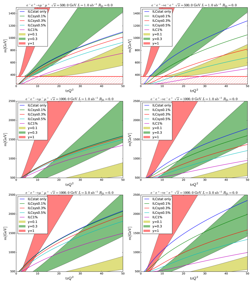
Figure 1: Mass reach for $R_{21}=0$. The ILC beam energy is $\sqrt{s}=500\mathrm{GeV}$ ($1\mathrm{TeV}$) for the upper figures (the middle and lower figures), while the integrated luminosity is $1\ {\rm ab}^{-1}$ ($3\ {\rm ab}^{-1}$) for the upper and middle figures (lower figures). Three figures on the left are ILC bounds from the $\mu^{+}\mu^{-}$ final state, and right figures are bounds from the $e^{+}e^{-}$ final state. The region below each solid line can be probed by the ILC with each systematic uncertainty. The yellow, green, and red bands show the region in which $\sigma(pp\to S\to\gamma\gamma)=3$ – $10$ fb is realized with $y=0.1$, $0.3$, and $1$, respectively.

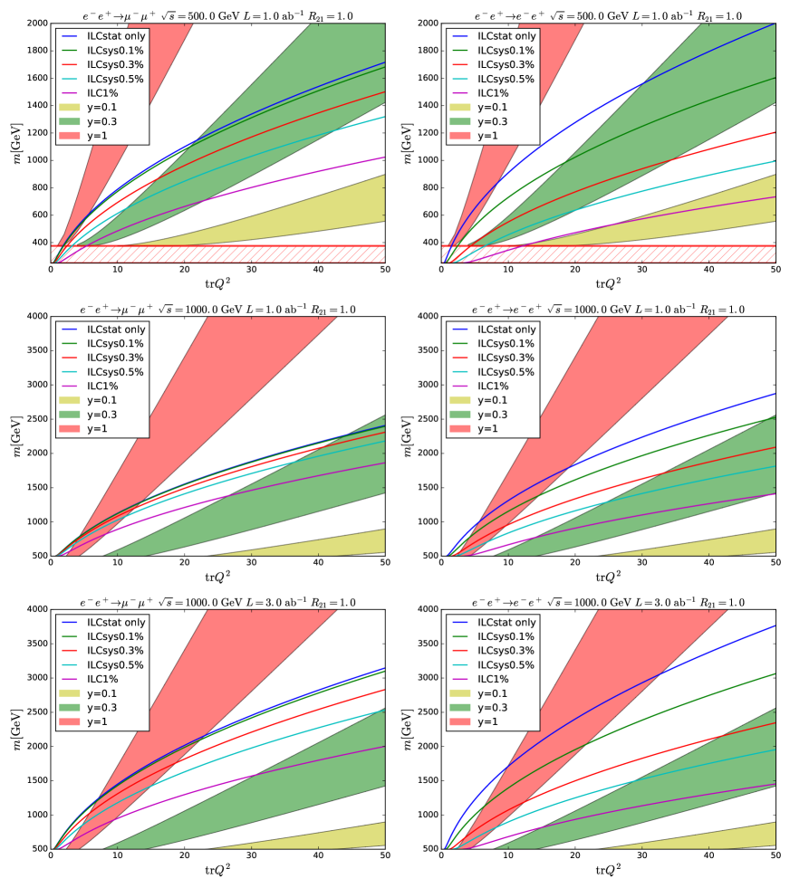
Figure 2: Same as Fig. 1, except for $R_{21}=1$.

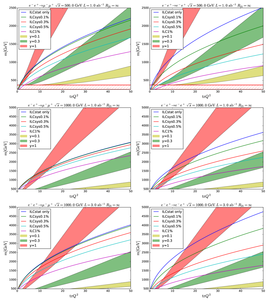
Figure 3: Same as Fig. 1, except for $R_{21}=\infty$, and the yellow, green, and red bands showing the region of $\sigma(pp\to S\to\gamma\gamma)=3$ – $7$ fb for $y=0.1$, $0.3$, and $1$, respectively. (See the discussion in the text.)

In Figs. 1 – 3, we show the contours of $\Delta\chi^{2}=2.71$, which gives 95% C.L. reach of the mass, on $\text{tr}Q^{2}$ vs. $m$ plane (solid lines). Each line corresponds to the systematic uncertainty of $\epsilon=0,0.1,0.3,0.5$, and $1\%$. In each figure, we shaded the regions at which $\sigma(pp\to S\to\gamma\gamma)$ becomes the relevant value to explain the diphoton excess for the Yukawa coupling $y=0.1$, 0.3, and 1. Here, we have assumed that the $S$ is a pseudo-scalar. As seen in the figures, the indirect probe at the ILC can cover a large parameter space of the diphoton models.

• Fig. 1 shows the case of $R_{21}=0$, which corresponds to SU(2) singlet. For instance, by measuring the cross sections of $e^{+}e^{-}\to\mu^{+}\mu^{-}$ and $e^{+}e^{-}\to e^{+}e^{-}$ with $\epsilon=0.1\%$, $\sqrt{s}=500\ \mathrm{GeV}$ and $L=1\ {\rm ab}^{-1}$ ($\sqrt{s}=1\ {\rm TeV}$ and $L=3\ {\rm ab}^{-1}$), the ILC can probe up to $m\simeq 500\ \mathrm{GeV}$ and $460\ \mathrm{GeV}$ ($960\ \mathrm{GeV}$ and $880\ \mathrm{GeV}$) for $\mathrm{tr}Q^{2}=10$, respectively.

• Fig. 2 shows the case of $R_{21}=1$, which corresponds to the case that the fermions has the same quantum numbers as those of the SM left-handed leptons, i.e., $({\bf 1},{\bf 2},1/2)$ for ${\rm SU}(3)\times{\rm SU}(2)\times{\rm U}(1)_{Y}$. The mass reach is larger than the case of $R_{21}=0$, because the SU(2) gauge coupling is larger than the U(1)_Y gauge coupling and that yields larger discrepancy from SM. By measuring the cross sections of $e^{+}e^{-}\to\mu^{+}\mu^{-}$ and $e^{+}e^{-}\to e^{+}e^{-}$ with $\epsilon=0.1\%$, $\sqrt{s}=500\ \mathrm{GeV}$ and $L=1\ {\rm ab}^{-1}$ ($\sqrt{s}=1\ {\rm TeV}$ and $L=3\ {\rm ab}^{-1}$), the ILC can probe up to $m\simeq 780\ \mathrm{GeV}$ and $730\ \mathrm{GeV}$ ($1430\ \mathrm{GeV}$ and $1390\ \mathrm{GeV}$) for $\mathrm{tr}Q^{2}=10$, respectively. Thus, the ILC will be able to reach the mass at the TeV scale if $\sqrt{s}\sim 1\ {\rm TeV}$ is available, and hence covers a large parameter space.

• Fig. 3 shows the case of $R_{21}=\infty$, which corresponds to the fermion with $Y=0$. In this case, as we can see, the fermions with their masses of a few TeV may be probed with $\sqrt{s}\sim 1\ {\rm TeV}$, and the mass reach becomes the largest among the examples we consider in this letter. Taking $\sqrt{s}=500\ \mathrm{GeV}$ and $L=1\ {\rm ab}^{-1}$ ($\sqrt{s}=1\ {\rm TeV}$ and $L=3\ {\rm ab}^{-1}$), $\epsilon=0.1\%$ and $\mathrm{tr}Q^{2}=10$, the ILC can probe up to $1000\ \mathrm{GeV}$ and $910\ \mathrm{GeV}$ ($1820\ \mathrm{GeV}$ and $1750\ \mathrm{GeV}$) by measuring the cross sections of $e^{+}e^{-}\to\mu^{+}\mu^{-}$ and $e^{+}e^{-}\to e^{+}e^{-}$, respectively. We should note that, in the case of $Y=0$, the decay of $S$ into other electroweak gauge bosons are enhanced. In particular, the ratio of the $Z\gamma$ to $\gamma\gamma$ decay rates become $\text{Br}(S\rightarrow Z\gamma)/\text{Br}(S\rightarrow\gamma\gamma)\simeq 6.3$. The 8 TeV run of the LHC has provided an upper bound of $\text{Br}(S\rightarrow Z\gamma)/\text{Br}(S\rightarrow\gamma\gamma)\lesssim 8.4\times[\sigma(pp\rightarrow S\rightarrow\gamma\gamma)/5\ {\rm fb}]^{-1}$ (see, e.g., [9]). Thus, in Fig. 3 we show the region of $\sigma(pp\rightarrow S\rightarrow\gamma\gamma)\leq 7\ {\rm fb}$.

Before closing this section, let us briefly comment on the possibilities to probe other scenarios. First, assuming $S$ is CP even, the charged particles in the loop for the diphoton signal can be scalars. Even in such a case, the charged scalars affect the ILC processes through their contributions to the vacuum polarizations. (See footnote 2.) We checked that a large parameter space of the diphoton models is probed also in such a case. Next, there is a different scenario that the 750 GeV resonance is a QCD bound state of vector-like quarks with a mass of about 375 GeV and a hypercharge $Y=-4/3$ [10]. This scenario corresponds to the point $(\text{tr}Q^{2},m)=(16/3,375~{}\text{GeV})$ in Fig. 1, which is within the reach of the ILC with $\sqrt{s}=500~{}\text{GeV}$.

4 Studying SU(2) and U(1)_Y quantum numbers

Now we consider how well we can distinguish different models containing new particles with different gauge quantum numbers. For this purpose, we use the fact that, for the process $e^{+}e^{-}\rightarrow\bar{f}f$ (with $f\neq e^{-}$), the effects of the new particles (with fixed $s$) are determined by only two parameters: $\delta\Pi_{BB}(s)$ and $\delta\Pi_{WW}(s)$. As one can understand from Eqs. (9) and (10), the relative size of $\delta\Pi_{BB}(s)$ and $\delta\Pi_{WW}(s)$ is sensitive to the gauge quantum numbers of the new particles. Importantly, the effects of $\delta\Pi_{BB}(s)$ and $\delta\Pi_{WW}(s)$ on the angular distributions are different. In the following, we discuss how well we can distinguish models behind the diphoton excess at the LHC by using the scattering process $e^{+}e^{-}\rightarrow\mu^{+}\mu^{-}$.

First, for the demonstration of the angular distribution with non-vanishing $\delta\Pi_{BB}(s)$ or $\delta\Pi_{WW}(s)$, let us define

$${\cal F}_{\mu^{+}\mu^{-}}(\cos\theta)\equiv\frac{[{d\sigma^{\rm SM+\psi}(e^{+}e^{-}\to\mu^{+}\mu^{-})}/{d\cos\theta}]-[{d\sigma^{\rm SM}(e^{+}e^{-}\to\mu^{+}\mu^{-})}/{d\cos\theta}]}{[{d\sigma^{\rm SM}(e^{+}e^{-}\to\mu^{+}\mu^{-})}/{d\cos\theta}]},$$ (23)

where $\sigma^{\rm SM}$ and $\sigma^{\rm SM+\psi}$ are cross sections in the SM and in the model with the new charged particles, respectively. In Fig. 4, we plot the above quantity as a function of $\cos\theta$ for $(\delta\Pi_{BB},\delta\Pi_{WW})=(-0.0029,0)$ and $(0,-0.0040)$. (See Table 1.) We can see that the angular distribution is affected differently in two cases. Thus, a precise study of the angular distributions provides constraints on $\delta\Pi_{BB}$ and $\delta\Pi_{WW}$.

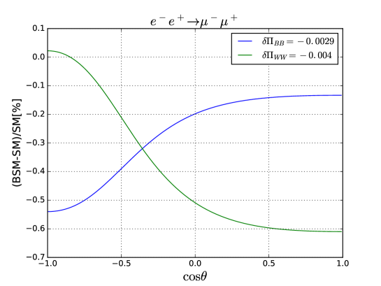
Figure 4: The deviation of the differential cross section from the Standard model. Blue and green lines show the cases with $(\delta\Pi_{BB},\delta\Pi_{WW})=(-0.0029,0)$ and $(0,-0.0040)$, respectively. We take $\sqrt{s}=500$GeV, $P_{-}=-80\%$ and $P_{+}=30\%$.

In order to study how well these two parameters are determined, we perform the following analysis:

1. We choose several sample points which can explain the diphoton excess. (See Table 1.)

2. For each sample point, we calculate the new particle contributions to the vacuum polarizations, which we denote by $\overline{\delta\Pi}_{BB}$ and $\overline{\delta\Pi}_{WW}$.

3. We estimate the ILC sensitivity for each sample point by using the following quantity:

   $$\Delta\chi^{2}(\delta\Pi_{BB},\delta\Pi_{WW};\overline{\delta\Pi}_{BB},\overline{\delta\Pi}_{WW})\equiv\sum_{i}\frac{(\overline{N}_{i}^{\rm SM+\psi}-N^{\rm SM+\psi})_{i}^{2}}{\overline{N}_{i}^{\rm SM+\psi}+(\epsilon\overline{N}_{i}^{\rm SM+\psi})^{2}},$$ (24)

   where $\overline{N}^{SM+\psi}$ and $N^{SM+\psi}$ are the number of $\mu^{+}\mu^{-}$ events in each bin evaluated with $(\overline{\delta\Pi}_{BB},\overline{\delta\Pi}_{WW})$ and $(\delta\Pi_{BB},\delta\Pi_{WW})$, respectively.

Sample points	1	2	3	4
Representation	$({\bf 1},{\bf 1},1)$	$({\bf 1},{\bf 3},0)$	$({\bf 1},{\bf 1},1)$	$({\bf 1},{\bf 3},0)$
$m_{\psi}$ [GeV]	400	400	600	600
$N$	7	3	7	3
$y$	0.3	0.5	0.5	1
$\Gamma(S\rightarrow\gamma\gamma)$ [MeV]	1.0	0.52	0.61	0.45
$\sqrt{s}$ [GeV]	500	500	1000	1000
$\overline{\delta\Pi}_{BB}(s)$	$-0.0029$	0	$-0.0066$	0
$\overline{\delta\Pi}_{WW}(s)$	0	$-0.004$	0	$-0.009$

Table 1: The parameters of the sample points for our numerical study: the representation for ${\rm SU}(3)\times{\rm SU}(2)\times{\rm U}(1)_{Y}$, the fermion mass, the multiplicity $N$, the Yukawa coupling, and $\Gamma(S\rightarrow\gamma\gamma)$. We use the sample points 1 and 2 (3 and 4) for the analysis with $\sqrt{s}=500\ {\rm GeV}$ ($1\ {\rm TeV}$). We also show the values of $\delta\Pi_{BB}(s)$ and $\delta\Pi_{WW}(s)$.

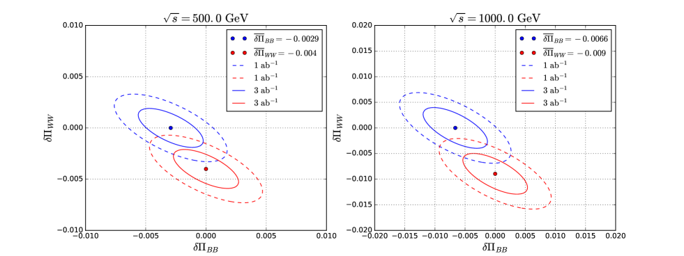
Figure 5: Contours of constant $\Delta\chi^{2}=5.99$ with the luminosity of $1\ {\rm ab}^{-1}$ (dashed) and $3\ {\rm ab}^{-1}$ (solid). The blue (red) contours are for Sample points 1 or 3 (2 or 4). Here, we take $\epsilon=0$.

In Fig. 5, the contours of constant $\Delta\chi^{2}(\delta\Pi_{BB},\delta\Pi_{WW};\overline{\delta\Pi}_{BB},\overline{\delta\Pi}_{WW})$ are presented on $\delta\Pi_{BB}$ vs. $\delta\Pi_{WW}$ plane. Here, we show $\Delta\chi^{2}=5.99$, which gives $95\ \%$ C.L. bounds on the $\delta\Pi_{BB}$ vs. $\delta\Pi_{WW}$ plane, taking the luminosity of $1\ {\rm ab}^{-1}$ and $3\ {\rm ab}^{-1}$. Here, we take $\epsilon=0$ to show the ultimate sensitivity. We can see that, with the precision measurements at the ILC, we will be able to obtain non-trivial constraint on the $\delta\Pi_{BB}$ vs. $\delta\Pi_{WW}$ plane. In addition, these results indicate that the ILC may be able to discriminate models containing new particles with various quantum numbers.

5 Summary and discussion

In this letter, we have studied the possibility of indirectly probing the charged particles which are responsible for the diphoton excess recently reported by the LHC. If the LHC diphoton excess indicates the existence of a new resonance $S$ with a mass of $\sim 750\ {\rm GeV}$, and also if it has a decay mode $S\rightarrow\gamma\gamma$, $S$ is likely to couple to new charged particles whose loop effects induce the coupling between $S$ and photon. Even if such charged particles are too heavy to be accessible with the ILC, they affect the scattering processes $e^{+}e^{-}\to f\bar{f}$ via vacuum polarizations of $\gamma$ and $Z$. With a precise study of the scattering processes, information about the vacuum polarization is obtained, from which the existence of the heavy charged particles can be probed.

We have quantitatively studied such an effect, and shown that the indirect probe of the charged particles is possible even if they are kinematically inaccessible at the ILC. The effects of the charged particles on the scattering process is insensitive to the strength of the interaction between $S$ and the charged particles, but it depends only on the mass, the multiplicity, and the SU(2)$\times$U(1)_Y representation of the new particles. We have also shown that the angular distributions are affected differently by the vacuum polarizations of SU(2) and U(1)_Y gauge bosons, which makes it possible to distinguish signals from new particles with different quantum numbers.

In our analysis, we have performed our analysis based on LO formulae of the scattering cross section to demonstrate the expected accuracy of the indirect probe. When such an analysis is performed with real data, however, higher order corrections should be properly taken into account in order to precisely predict the angular distribution of the final-state fermions of the scattering processes. In addition, we have used only the scattering processes with leptonic final states. We may also be able to use the quark final states taking into account the QCD corrections.

Should the diphoton excess persists with more data at the LHC, it is of great importance to probe the physics behind it. The precision measurements at the ILC will provide good indirect probes of the origin of the diphoton excess, which are complementary to the study at the LHC.

References

- [1] The ATLAS collaboration, “Search for resonances decaying to photon pairs in 3.2 fb-1 of collisions at = 13 TeV with the ATLAS detector,” ATLAS-CONF-2015-081.
- [2] CMS Collaboration, “Search for new physics in high mass diphoton events in proton-proton collisions at 13TeV,” CMS-PAS-EXO-15-004.
- [3] T. Behnke et al., arXiv:1306.6327 [physics.acc-ph].
-
[4]
H. Baer et al.,
arXiv:1306.6352 [hep-ph].
C. Adolphsen et al., arXiv:1306.6353 [physics.acc-ph].
C. Adolphsen et al., arXiv:1306.6328 [physics.acc-ph].
T. Behnke et al., arXiv:1306.6329 [physics.ins-det]. - [5] K. Harigaya, K. Ichikawa, A. Kundu, S. Matsumoto and S. Shirai, JHEP 1509 (2015) 105 [arXiv:1504.03402 [hep-ph]].
-
[6]
H. Ito, T. Moroi and Y. Takaesu,
Phys. Lett. B 756 (2016) 147
[arXiv:1601.01144 [hep-ph]].
N. Sonmez, arXiv:1601.01837 [hep-ph].
A. Djouadi, J. Ellis, R. Godbole and J. Quevillon, JHEP 1603 (2016) 205 [arXiv:1601.03696 [hep-ph]].
M. He, X. G. He and Y. Tang, arXiv:1603.00287 [hep-ph].
H. Ito and T. Moroi, arXiv:1604.04076 [hep-ph]. - [7] A. D. Martin, W. J. Stirling, R. S. Thorne and G. Watt, Eur. Phys. J. C 63 (2009) 189 [arXiv:0901.0002 [hep-ph]].
- [8] N. Kumar and S. P. Martin, Phys. Rev. D 92 (2015) no.11, 115018 [arXiv:1510.03456 [hep-ph]].
- [9] S. Knapen, T. Melia, M. Papucci and K. Zurek, Phys. Rev. D 93 (2016) no.7, 075020 [arXiv:1512.04928 [hep-ph]].
-
[10]
C. Han, K. Ichikawa, S. Matsumoto, M. M. Nojiri and M. Takeuchi,
arXiv:1602.08100 [hep-ph].
Y. Kats and M. Strassler, arXiv:1602.08819 [hep-ph].
K. Hamaguchi and S. P. Liew, arXiv:1604.07828 [hep-ph].