Jet-dilepton conversion from an anisotropic quark-gluon plasma

Abstract

We calculate the yield of lepton pair production from jet-plasma interaction where the plasma is anisotropic in momentum space. We compare both the $M$ and $p_{T}$ distributions from such process with the Drell-Yan contribution. It is observed that the invariant mass distribution of lepton pair from such process dominate over the Drell-Yan up to $3$ GeV at RHIC and up to $10$ GeV at LHC. Moreover, it is found that the contribution from anistropic quark gluon plasma (AQGP) increases marginally compared to the isotropic QGP. In case of $p_{T}$-distribution we observe an increase by a factor of $3-4$ in the entire $p_{T}$-range at RHIC for AQGP. However, at LHC the change in the $p_{T}$-distribution is marginal as compared to the isotropic case.

I Introduction

The primary goal of heavy-ion collisions at Relativistic Heavy Ion Collider (RHIC) at BNL and Large Hadron Collider (LHC) at CERN is to establish the existence of a transient phase consisting of quarks, anti-quarks and gluons known as Quark Gluon Plasma (QGP). Since such a phase lasts for a few $fm/c$, it is impossible to observe it directly. Thus, various indirect probes have been proposed in the literature prd44 ; zpc53 ; prc53 ; prd58 ; jhep0112 ; prd34 ; zpc46 ; prl70a ; npa566 ; plb331 ; plb178 ; prc53a . Electromagnetic probes is one of them. The advantage of such probe is that once these are produced they can escape the interaction zone without much distortion in their energy and momentum. They, thus carry the information of the collision dynamics very effectively. Photons and dileptons are produced throughout the evaluation process of the collisions. In the low and intermediate mass region, lepton pair are produced from the $q\bar{q}\rightarrow l^{+}l^{-}$ process (thermal) and from various hadronic reactions and decay. In the high mass region, there is the contribution from Drell-Yan process, which can be calculated from pQCD. Another important contribution in this invariant mass region is the jet-dilepton conversion in the QGP. Several authors prc67 ; prc74 ; npa865 ; prc92 have estimated this contribution where a jet quark (anti-quark) interact with a thermal anti-quark (quark) to produce a large mass lepton pair. It is to be noted that before annihilation of a $q~{}(\bar{q})$ jet with a thermal $\bar{q}~{}(q)$, the $q~{}(\bar{q})$ jet may lose energy. Such possibility has also been considered in Refs prc74 ; npa865 ; prc92 . It has been observed in all those calculation that the magnitude of this mechanism is order of magnitude larger than the thermal processes and is of the same order of the Drell-Yan processes prl25 . It is to be noted that in all those calculations an isotropic plasma has been assumed to be formed. But the most difficult problem lies in the determination of isotropization and thermalization time scales ($\tau_{\rm iso}$ and $\tau_{\rm therm}$ ) of the QGP. Studies on elliptic flow (upto about $p_{T}\sim 1.5−2$ GeV) using ideal hydrodynamics indicate that the matter produced in such collisions becomes isotropic with $\tau_{\rm iso}\sim 0.6$ fm/c plb503 . On the contrary, perturbative estimates yield much slower thermalization of QGP plb502 ; prc71 ; jpg34 . However, recent hydrodynamical studies prc78a have shown that due to the poor knowledge of the initial conditions, there is a sizable amount of uncertainty in the estimation of thermalization or isotropization time. The other uncertain parameters are the transition temperature $T_{c}$, the spatial profile, and the effects of flow. Thus it is necessary to find suitable probes which are sensitive to these parameters. As mentioned earlier electromagnetic probes have long been considered to be one of the most promising tools to characterize the initial state of the collisions prd34 ; zpc46 ; prl70a ; npa566 ; plb331 . Dileptons (photon as well) can be one such observables. In the early stages of heavy ion collisions, due to the rapid longitudinal expansion the plasma after formation in isotropic phase, may become anisotropic prd62 ; prd68 ; prd70 ; jhep08 ; prd70a ; prl94 ; prd72 ; prd73 ; ahep . As a result the momentum distribution of the plasma particles become anisotropic in momentum space. The author in Ref prc78 have calculated the ”medium” dilepton yield for various isotropization times and compared it with Drell-Yan and jet-thermal processes. It is shown that the effect of the anisotropy cannot be neglected while calculating $M-$ distribution and $p_{T}-$ distribution. In fact in certain kinematic region this contribution is comparable to Drell-Yan as well as jet-thermal process. Jet-photon conversion in the AQGP has been calculated in Ref jpg37 with $p_{T}$ up to $14$ GeV to extract the isotropization time. Also in intermediate and low $p_{T}$ the photon transverse momentum distribution has been calculated to infer about the isotropization time scale prc79 . It is to be noted that the extracted values of $\tau_{\rm iso}$ from the above two cases are consistent. To the best of our knowledge, the contribution of the jet-dilepton conversion in AQGP has not been done so far. It is, thus, our purpose to estimate the dilepton yield from jet-plasma interaction in the present work. To keep the things simple in this work, we shall not include the energy loss of the jet in the AQGP.

It should be noted that in absence of any precise knowledge about the dynamics at early time of the collision, one can introduce phenomenological models to describe the evolution of the pre-equilibrium phase. In this work, we will use one such model, proposed in Ref. prl100 ; prc78 ; prc84 , for the time dependence of the anisotropy parameter, $\xi(\tau)$, and hard momentum scale, $p_{\rm hard}(\tau)$. This model introduces four parameters to parameterize the ignorance of pre-equilibrium dynamics: the parton formation time ($\tau_{i}$), the isotropization time ($\tau_{\rm iso}$ ), which is the time when the system starts to undergo ideal hydrodynamical expansion and $\gamma$ sets the sharpness of the transition to hydrodynamical behavior. The fourth parameter $\delta$ is introduced to characterize the nature of pre-equilibrium anisotropy i.e. whether the pre-equilibrium phase is non-interacting or collisionally broadened.

The plane of the paper is the following. In the next section we describe the formalism of jet-conversion dilepton production in AQGP. Jet-production and Drell-Yan process will be discussed in section III. We present a brief discussion on space-time evolution of AQGP in section IV. Section V will be devoted to present the results. Finally, we summarize in section VI.

II Formalism

According to the relativistic kinetic theory, the dilepton production rate at leading order in the coupling $\alpha$, is given by plb283 ; prl70 ; plb331 :

$$\frac{dR^{l^{+}l^{-}}}{d^{4}P}=\int\frac{d^{3}{\bf p}_{1}}{(2\pi)^{3}}\frac{d^{3}{\bf p}_{2}}{(2\pi)^{3}}f_{q/{\bar{q}}}({\bf p}_{1})f_{\rm jet}({\bf p}_{2})\,v_{12}\,\sigma^{l^{+}l^{-}}_{q{\bar{q}}}\delta^{(4)}(P-p_{1}-p_{2})$$ (1)

where $f_{\rm jet}$ and $f_{q/{\bar{q}}}$ are the phase space distribution of the jet quarks/anti-quarks and medium quarks/anti-quarks respectively. The total cross section of the $q\bar{q}\rightarrow l^{+}l^{-}$ interaction is given by

$$\sigma^{l^{+}l^{-}}_{q{\bar{q}}}=\frac{4\pi}{3}\frac{\alpha^{2}}{M^{2}}N_{c}N_{s}(1+\frac{2m_{l}^{2}}{M^{2}})(1-\frac{4m_{l}^{2}}{M^{2}})^{1/2}\sum_{q}e^{2}_{q},$$ (2)

where $N_{c}$ and $N_{s}$ are the color factor and spin factor, respectively. $m_{l}$ is the mass of lepton and $M$ is the invarient mass of the lepton pair which is much greater than the dilepton mass. So we can easily ignore the lepton mass and we find $\sigma^{l^{+}l^{-}}_{q{\bar{q}}}=\frac{4\pi\alpha^{2}}{3M^{2}}N_{c}N_{s}\sum_{q}e^{2}_{q}$. We also assume that the distribution function of quarks and anti-quarks is the same. $v_{12}$ is the relative velocity between the jet quark and medium quark/anti-quark:

$$v_{12}=\frac{(p_{1}+p_{2})^{2}}{2E_{1}E_{2}}.$$ (3)

In this work we consider the medium is anisotropic in momentum space so that the anisotropic distribution function can be obtained from an arbitrary isotropic distribution by squeezing or stretching along the preferred direction in the momentum space prd68 :

$$f_{q/{\bar{q}}}({\bf p},\xi,p_{\rm hard})=f_{q/{\bar{q}}}(\sqrt{{\bf p}^{2}+\xi(\tau)(\bf{p}.\hat{{\bf n}})^{2}},p_{\rm hard}(\tau)),$$ (4)

where $\hat{\bf n}$ is the direction of anisotropy, $p_{\rm hard}(\tau)$ is a time-dependent hard momentum scale and $\xi(\tau)$ is a time-dependent parameter reflecting the strength of the momentum anisotropy. In isotropic case, where $\xi=0$, $p_{\rm hard}$ can be recognized with the plasma temperature $T$.

The phase space distribution function for a jet, assuming the constant transverse density of the nucleus is given by prl90 ; prc74 :

$$f_{\rm jet}({\bf p})=\frac{(2\pi)^{3}}{g_{q}}\frac{{\mathcal{P}}(|\vec{\omega}_{r}|)}{\sqrt{\tau_{i}^{2}-z_{0}^{2}}}\frac{1}{p_{T}}\frac{dN_{\rm jet}}{d^{2}p_{T}dy}\delta(z_{0})$$ (5)

where $g_{q}=2\times 3$ is the spin and color degeneracy factor, $\tau_{i}\sim 1/p_{T}$ is the formation time of the quark or anti-quark jet, and $z_{0}$ is its position in the QGP expansion direction. ${\mathcal{P}}(|\vec{\omega}_{r}|)$ is the initial jet production probability distribution at the radial position $\vec{\omega}_{r}$ in the plane $z_{0}$, where

$$|\vec{\omega}_{r}| = [\vec{r}-(\tau-\tau_{i})\frac{\vec{p}}{|\vec{p}|}].\vec{r}$$ (6)

$$= \sqrt{(r\cos\phi-\tau)^{2}+r^{2}\sin^{2}\phi}~{}~{}~{}{\rm for}~{}\tau_{i}\sim 0$$

and $\phi$ is the angle in the plane $z_{0}$ between the direction of the virtual photon and the position where this virtual photon has been produced.

Eq. (1) can be written as

$$\frac{dR^{l^{+}l^{-}}}{d^{4}P} = \frac{5\alpha^{2}}{72\pi^{5}}\int\frac{d^{3}{\bf p}_{1}}{E_{p_{1}}}\frac{d^{3}{\bf p}_{2}}{E_{p_{2}}}f_{q/{\bar{q}}}({\bf p}_{1},\xi,p_{\rm hard})f_{\rm jet}({\bf p}_{2})\delta^{(4)}(P-p_{1}-p_{2})$$ (7)

$$= \frac{5\alpha^{2}}{72\pi^{5}}\int\frac{d^{3}{\bf p}_{1}}{E_{p_{1}}E_{p_{1}}}f_{q/{\bar{q}}}({\bf p}_{1},\xi,p_{\rm hard})f_{\rm jet}({\bf p}-{\bf p}_{1})\delta(E-E_{p_{1}}-E_{p_{2}})\Bigg{|}_{{\bf p}_{2}={\bf P}-{\bf p}_{2}}$$

If we choose

$${\bf p}_{1} = p_{1}(\sin\theta_{p_{1}}\cos\phi_{p_{1}},\sin\theta_{p_{1}}\sin\phi_{p_{1}},\cos\theta_{p_{1}}),$$

$${\bf P} = P(\sin\theta_{P}\cos\phi_{P},\sin\theta_{P}\sin\phi_{P},\cos\theta_{P})$$ (8)

and anisotropy vector $\hat{\bf n}$ along the $z$ direction, the $\delta$ function can be expressed as

$$\delta(E-E_{p_{1}}-E_{p_{2}})=2(E-p_{1})\chi^{-1}\Theta(\chi)\sum_{i}^{2}\delta(\phi_{i}-\phi_{p_{1}}),$$ (9)

with $\chi=\Bigg{[}4P^{2}p_{1}^{2}\sin^{2}\theta_{P}\sin^{2}\theta_{p_{1}}-[2p_{1}(E-P\cos\theta_{P}\cos\theta_{p_{1}})-M^{2}]^{2}\Bigg{]}>0$ and the angle $\phi_{i}$ can be found by the solutions to the following equation:

$$\cos(\phi_{i}-\phi_{p_{1}})=\frac{2p_{1}(E-P\cos\theta_{P}\cos\theta_{p_{1}})-M^{2}}{2Pp_{1}\sin\theta_{P}\sin\theta_{p_{1}}}$$ (10)

Eq. (7) can now be written as

$$\frac{dR^{l^{+}l^{-}}}{d^{4}P} = \frac{5\alpha^{2}}{18\pi^{5}}\int_{-1}^{+1}d(\cos\theta_{p_{1}})\int^{a_{-}}_{a_{+}}\frac{dp_{1}}{\sqrt{\chi}}p_{1}f_{q/{\bar{q}}}(\sqrt{{\bf p}_{1}^{2}(1+\xi\cos^{2}\theta_{p_{1}})},p_{\rm hard})f_{\rm jet}({\bf p}-{\bf p}_{1})$$ (11)

with

$$a_{\pm}=\frac{M^{2}}{2[E-P\cos(\theta_{P}\pm\theta_{p_{1}})]}$$ (12)

Now, the dilepton production rate $R$ is defined as the total number of lepton pair emitted from the 4-dimensional space-time element $d^{4}x=\tau\,d\tau\,d\eta\,d^{2}x_{\perp}$ with $R=dN/d^{4}x$. Here, $\tau=\sqrt{t^{2}-z^{2}}$ is the longitudinal proper time, $\eta=\tanh^{-1}(z/t)$ is the space-time rapidity, and ${\bf x}_{\perp}$ is a two-vector containing the transverse coordinates.

The total dilepton spectrum is given by a full space-time integration:

$$\frac{dN^{l^{+}l^{-}}}{dM^{2}dy} = \int_{p^{\rm min}_{T}}^{p^{\rm max}_{T}}d^{2}p_{T}\int_{\tau_{i}}^{\tau_{f}}\tau d\tau\int_{0}^{R_{\perp}}rdr\int_{0}^{\pi}d\phi\int_{-\infty}^{+\infty}d\eta\frac{dR^{l^{+}l^{-}}}{d^{4}P}(E=m_{T}\cosh(y-\eta)),$$ (13)

$$\frac{dN^{l^{+}l^{-}}}{d^{2}p_{T}dy} = \int_{M^{\rm min}}^{M^{\rm max}}dM^{2}\int_{\tau_{i}}^{\tau_{f}}\tau d\tau\int_{0}^{R_{\perp}}rdr\int_{0}^{\pi}d\phi\int_{-\infty}^{+\infty}d\eta\frac{dR^{l^{+}l^{-}}}{d^{4}P}(E=m_{T}\cosh(y-\eta)),$$ (14)

where $R_{\perp}=1.2[<N_{\rm part}>/2]^{1/3}$ is the transverse dimension of the system amd $m_{T}$ is the transverse mass of the pair. We have assumed that the plasma is formed at time $\tau_{i}$ and it undergoes a phase transition at transition temperature ($T_{c}$) which begins at the time $\tau_{f}$. $\tau_{f}$ is obtained by using the condition $p_{\rm hard}(\tau=\tau_{f})=T_{c}$. The energy of the dilepton pair in the fluid rest has to be understood as $E=m_{T}\cosh(y-\eta)$. Now the $\phi$ integration can be done as follows:

$$\int_{0}^{\pi}d\phi\,{\mathcal{P}}({|\vec{\omega}_{r}|})=\begin{cases}0,&r^{2}+\tau^{2}-2\tau r\,>\,R^{2}_{\perp}\\ \frac{4}{R^{2}_{\perp}}(1-\frac{r^{2}+\tau^{2}}{R^{2}_{\perp}}),&r^{2}+\tau^{2}+2\tau r\,<\,R^{2}_{\perp}\\ \frac{4u_{0}}{\pi R^{2}_{\perp}}(1-\frac{r^{2}+\tau^{2}}{R^{2}_{\perp}})+\frac{8\tau r}{\pi R^{4}_{\perp}}\sin(u_{0})&{\rm otherwise},\end{cases}$$ (15)

where

$$u_{0}=\arccos(\frac{r^{2}+\tau^{2}-R^{2}_{\perp}}{2\tau r}).$$ (16)

III Jets Production and Drell-Yan process

The differential cross-section for the jet production in hadron-hadron collision ($A+B\rightarrow{\rm jets}+X$) can be written as RMP59

$$\frac{d\sigma_{\rm jet}}{d^{2}p_{T}dy}=K\sum_{a,b}\int_{x_{a}^{\rm min}}^{1}dx_{a}G_{a/A}(x_{a},Q^{2})G_{b/B}(x_{b},Q^{2})\frac{x_{a}x_{b}}{x_{a}-\frac{p_{T}}{\sqrt{s}}e^{y}}\frac{1}{\pi}\frac{d{\hat{\sigma}}_{ab\rightarrow{\rm cd}}}{d{\hat{t}}}$$ (17)

where $\sqrt{s}$ is the total energy in the center-of-mass and $x_{a}~{}(x_{b})$ is the momentum fraction of the parton $a~{}(b)$ of the nucleon $A~{}(B)$. $G_{a/A}~{}(G_{b/B})$ is the parton distribution function (PDF) of the incoming parton $a~{}(b)$ in the incident hadron $A~{}(B)$. $K$ factor is used to account the next-to-leading (NLO) order effect. The minimum value of $x_{a}$ is

$$x^{\rm min}_{a}=\frac{p_{T}e^{y}}{\sqrt{s}-p_{T}e^{-y}}.$$ (18)

The value of the momentum fraction $x_{b}$ can be written as

$$x_{b}=\frac{x_{a}p_{T}e^{-y}}{x_{a}\sqrt{s}-p_{T}e^{y}}.$$ (19)

$\frac{d{\hat{\sigma}}_{ab\rightarrow{\rm cd}}}{d{\hat{t}}}$ is the cross section of parton collision at leading order. These process are: $qq\rightarrow qq$, $q\bar{q}\rightarrow q\bar{q}$, $q\bar{q}\rightarrow q^{\prime}\bar{q}^{\prime}$, $qq^{\prime}\rightarrow qq^{\prime}$, $q\bar{q}^{\prime}\rightarrow q\bar{q}^{\prime}$, $qg\rightarrow qg$, and $gg\rightarrow q\bar{q}$. The yield for producing jets in the heavy-ion collision is given by

$$\frac{dN_{\rm jet}}{d^{2}p_{T}dy}=T_{\rm AA}\frac{d\sigma_{\rm jet}}{d^{2}p_{T}dy}\Bigg{|}_{y=0}$$ (20)

where $T_{\rm AA}=9A^{2}/8\pi R^{2}_{\perp}$ is the nuclear thickness function for zero impact parameter prl90 . The $p_{T}$ distribution of the jet quarks in the central rapidity region ($y=0$) was computed in prc67 and parameterized as

$$\frac{dN_{\rm jet}}{d^{2}p_{T}dy}{\Bigg{|}}_{y=0}=K\frac{a}{(1+\frac{p_{T}}{b})^{c}}.$$ (21)

Numerical values for the parameters $a$, $b$ and $c$ are listed in Ref.prc67 .

The cross-section for the Drell-Yan process (LO) is given by plb78

$$\frac{dN_{\rm DY}}{dM^{2}dy}=T_{\rm AA}K_{\rm DY}\frac{4\pi\alpha}{9M^{4}}\sum_{q}e^{2}_{q}\big{[}x_{1}G_{q/A}(x_{1},Q^{2})x_{2}G_{\bar{q}/B}(x_{2},Q^{2})+\sum_{q}e^{2}_{q}\big{[}x_{1}G_{\bar{q}/A}(x_{1},Q^{2})x_{2}G_{q/B}(x_{2},Q^{2})\big{]}$$ (22)

where the momentum fractions with rapidity $y$ are $x_{1}=\frac{M}{\sqrt{s}}e^{y}$, $x_{2}=\frac{M}{\sqrt{s}}e^{-y}$. $K_{\rm DY}$ factor of 1.5 is used to account for the NLO correction plb473 .

IV Space-time evaluation

For the case of expanding plasma, we will be required to specify a proper-time dependence of the anisotropy parameter, $\xi$ and the hard momentum scale, $p_{\rm hard}$. In our calculation, we assume an isotropic plasma is formed at initial time $\tau_{i}$ and initial temperature $T_{i}$. The initial rapid expansion of the matter along the longitudinal direction causes faster cooling in this direction than in the transverse direction plb502 and as result, a local momentum-space anisotropy occurs and remains until $\tau=\tau_{\rm iso}$. In this work, we shall follow the work of ref prl100 ; prc78 to evaluate the dilepton production rate from the first few Fermi of the plasma evolution. According to this model there can be three possible scenarios : (i) $\tau_{i}=\tau_{\rm iso}$, the system evolves hydrodynamically so that $\xi(\tau)=0$ and we can identify the hard momentum scale with the plasma temperature so that $p_{\rm hard}(\tau)=T(\tau)=T_{0}(\tau_{i}/\tau)^{1/3}$, (ii)$\tau_{\rm iso}\rightarrow\infty$, the system never comes to equilibrium, (iii)$\tau_{iso}\geq\tau_{i}$ and $\tau_{\rm iso}$ is finite, one should devise a time evolution model for $\xi(\tau)$ and $p_{\rm hard}(\tau)$ which smoothly interpolates between pre-equilibrium anisotropy and hydrodynamics and we shall follow scenario (iii). The time dependent parameters ($\xi,p_{\rm hard}$), are obtained in terms of a smeared step function prl100 :

$$\lambda(\tau)=\frac{1}{2}(\tanh[\gamma(\tau-\tau_{iso})/\tau_{i}]+1).$$ (23)

where the transition width, $\gamma^{-1}$ is introduced to take into account the smooth transition between non-equilibrium and hydrodynamical evolution at $\tau=\tau_{\rm iso}$. It is clearly seen that for $\tau\,<<\,\tau_{\rm iso}$, we have $\lambda\rightarrow 0$, corresponding to anisotropic evolution and for $\tau\,>>\,\tau_{\rm iso}$, $\lambda\rightarrow 1$ which corresponds to hydrodynamical evolution.

With this, the time dependence of relevant quantities are as follows prl100 ; prc78 :

$$p_{\rm hard}(\tau) = T_{i}\,\left[{\cal U(\tau)}/{\cal U}(\tau_{i})\right]^{1/3},$$

$$\xi(\tau) = a^{\delta[1-\lambda(\tau)]}-1,$$ (24)

where ${\mathcal{U}}(\tau)\equiv\left[{\mathcal{R}}\left(a_{\rm iso}^{\delta}-1\right)\right]^{3\lambda(\tau)/4}\left(a_{\rm iso}/a\right)^{1-\delta[1-\lambda(\tau)]/2}$, $a\equiv\tau/\tau_{i}$ and $a_{\rm iso}\equiv\tau_{\rm iso}/\tau_{i}$ and ${\mathcal{R}}(x)=\frac{1}{2}(\frac{1}{1+\xi}+\frac{\arctan\sqrt{\xi}}{\sqrt{\xi}}).$ In the present work, we have used a free streaming interpolating model that interpolates between early-time $1+1$ dimensional longitudinal free streaming and late-time $1+1$ dimensional ideal hydrodynamic expansion by choosing $\delta=2$.

As the colliding nuclei do have a transverse density profile, we assume that the initial temperature profile is given by prc72

$$T_{i}(r)=T_{i}\,\left[2\left(1-r^{2}/R_{A}^{2}\right)\right]^{1/4}$$ (25)

Using Eqs.(24) and (25) we obtain the profile of the hard momentum scale as

$$p_{\rm hard}(\tau,r)=T_{i}\,\left[2\left(1-r^{2}/R_{A}^{2}\right)\right]^{1/4}{\bar{\cal U}}^{c_{s}^{2}}(\tau).$$ (26)

In case of isentropic expansion the initial temperature ($T_{i}$) and thermalization time ($\tau_{i}$) can be related to the observed particle rapidity density by the following equation prd32 :

$$T_{i}^{3}(b_{m})\tau_{i}=\frac{2\pi^{4}}{45\zeta(3)}\frac{1}{\pi R_{\perp}}\frac{1}{4a_{k}}<\frac{dN}{dy}(b_{m})>,$$ (27)

where $\frac{dN}{dy}(b_{m})$ is the hadron multiplicity for a given centrality class with maximum impact parameter $b_{m}$, $R_{\perp}$ is the transverse dimension of the system, $\zeta(3)$ is the Riemann zeta function, and $a_{k}=(\pi^{2}/90)g_{k}$ for a plasma of massless u, d and s quarks and gluons, where $g_{k}=42.25$.

V Results

For central Au $+$ Au collision at $\sqrt{S_{NN}}=200$ GeV we fix our initial conditions to be $T_{i}=446$ MeV and $\tau_{i}=0.147$ fm/c for the plasma phase. For the LHC at $\sqrt{S_{NN}}=5.5$ TeV, our initial conditions are $T_{i}=845$ MeV and $\tau_{i}=0.088$ fm/c.

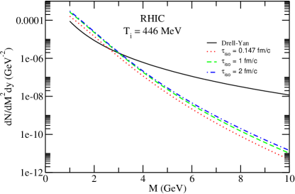
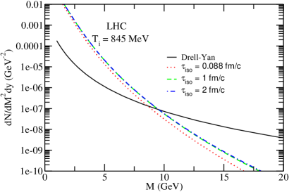
Figure 1: Dilepton yield for central Au $+$ Au collisions at $\sqrt{S_{NN}}=200$ GeV (left panel) and for central Pb $+$ Pb collisions at $\sqrt{S_{NN}}=5.5$ TeV (right panel).

Using the above initial conditions, we display the invariant mass distribution for RHIC (left panel) and LHC (right panel) energies in Fig. (1). It is found that the contribution from jet-dilepton conversion in isotropic plasma dominates over the Drell-Yan contribution up to $M\sim 2.5$ GeV (see left panel). However, when anisotropy is introduced this threshold increases to $M=3$ GeV irrespective of the values of the isotropization time. For LHC energies (right panel) this threshold increases up to $M\sim 10$ GeV providing an expanded window at LHC where jet-conversion dilepton could be observed when anisotropy is taken into account. The $p_{T}$-distribution is shown in Fig. (2) where we find that the effect of anisotropy at RHIC energies is substantial (increases by a factor of $4$). Surprisingly, at LHC energies the effect is not substantial. In Fig. (3) we compare the contribution from jet-dilepton conversion with the medium dilepton prc78 , where $f_{\rm jet}(\bf{p_{2}})$ in Eq. (1) is replaced by $f_{\bar{q}/q}({\bf p_{2}})$. It is found that both for the RHIC and LHC energies at various $\tau_{\rm iso}$, the medium dilepton always remains below the jet-dilepton conversion in AQGP.

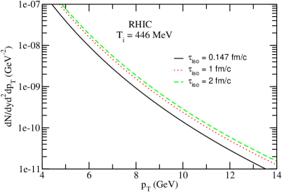
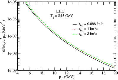
Figure 2: $p_{T}$ distribution of the jet-conversion dilepton, integrated in the range $0.5\,<\,M\,<1$ GeV, for the RHIC (left panel) and the LHC (right panel).

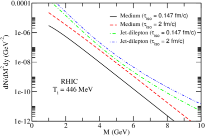
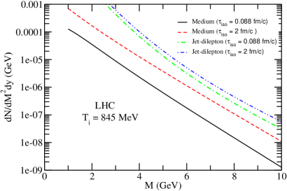
Figure 3: Collisionally broadened interpolating model dilepton yield and jet-conversion dilepton yield as a function of invariant mass in central Au $+$ Au collisions at $\sqrt{S_{NN}}=200$ GeV (left panel) and for central Pb $+$ Pb collisions at $\sqrt{S_{NN}}=5.5$ TeV (right panel).

VI Summary and Discussion

In this work we have calculated the contribution of lepton pair production in high mass region from jet-plasma interactions in AQGP. For the simplicity, (1+1)d anisotropic hydrodynamics has been used as the effect of transverse expansion will be marginal in the early stage of the collision (note that momentum-space anisotropy is an early time phenomenon). It is found that the threshold value of $M$ beyond which DY process dominates over jet-conversion dilepton increases marginally with the introduction of momentum-space anisotropy both for RHIC and LHC. However, we do not find any appreciable change in the $p_{T}$ distribution at LHC energies even if the anisotropy is introduced. We have also shows that the medium dilepton contribution always remains below the dilepton from the jet plasma interaction. In fact, the former is less than by a factor $4-10$ depending upon $\tau_{\rm iso}$ and $p_{T}$. Finally, in the present calculation we have not included the energy loss of the energetic jets which we propose to report elsewhere AM . We are also in the process of applying (1+3)d anisotropic hydrodynamics to estimate the jet-conversion dilepton from anisotropic quark-gluon plasma.

References

- (1) J. Kapusta, P. Lichard and D. Seibert, Phys. Rev. D 44, 2774 (1991), Erratum ibid 47, 4171 (1993).
- (2) R. Baier, H. Nakkagawa, A. Niegawa and K. Redlich, Z. Phys. C 53, 433 (1992).
- (3) P. K. Roy, D. Pal, S. Sarkar, D. K. Srivastava, and B. Sinha, Phys. Rev. C 53 2364 (1996).
- (4) P. Aurenche, F. Gelis, H. Zaraket, and R. Kobes, Phys. Rev. D 58, 085003 (1998).
- (5) P. Arnold, G. D. Moore and L. G. Yaffe, JHEP 0112, 009 (2001).
- (6) K. Kajantie, J. Kapusta, L. Mclerran, A. Mekjian, Phys. Rev. D 34, 2746 (1986).
- (7) K. J. Eskola and J. Lindfors, Z. Phys. C 46, 141 (1990).
- (8) K. Geiger and J. I. Kapusta, Phys. Rev. Lett. 70 1920 (1993).
- (9) B. Kampfer and O. P. Pavlenko, Nucl. Phys. A 566, 351 (1994).
- (10) M. Strickland Phys. Lett. B 331 (1994) 245.
- (11) H. Satz and T. Matsui, Phys. Lett. B178, 416 (1986).
- (12) X. M. Xu, D. Kharzeev, H. Satz, and X. N. Wang, Phys. Rev. C 53, 3051 (1996).
- (13) D. K. Srivastava, C. Gale, R. J. Fries, Phys. Rev. C 67 034903 (2003).
- (14) S. Turbide, C. Gale, D. K. Srivastava, R. J. Fries, Phys. Rev. C 74 014903 (2006).
- (15) Yong-Ping Fu and Yun-De Li, Nucl. Phys. A 865 76 (2011).
- (16) Yong-Ping Fu and Q. Xi Phys. Rev. C 92, 024914 (2015).
- (17) S. D. Drell and T. M. Yan, Phys. Rev. Lett. 25, 316 (1970).
- (18) P. Huovinen, P. F. Kolb, U. W. Heinz, P. V. Ruuskanen and S. A. Voloshin, Phys. Lett. B503, 58 (2001).
- (19) R. Baier, A. H. Mueller, D. Schiff and D. T. Son, Phys. Lett. B502, 51 (2001).
- (20) Z. Xu and C. Greiner, Phys. Rev. C 71, 064901 (2005).
- (21) M. Strickland, J. Phys. G 34, S429 (2007).
- (22) M. Luzum and P. Romatschke Phys. Rev. C 78, 034915 (2008), Erratum ibid 79, 039903 (2009).
- (23) S. Mrowczynski and M. H. Thoma, Phys. Rev. D 62, 036011 (2000).
- (24) P. Romatschke and M. Strickland, Phys. Rev. D 68 036004 (2003).
- (25) P. Romatschke and M. Strickland, Phys. Rev. D 70 116006 (2004).
- (26) P. Arnold, J. Lenaghan, and G. D. Moore, JHEP 08, 002 (2003).
- (27) S. Mrowczynski, A. Rebhan and M. Strickland, Phys. Rev. D 70, 025004 (2004).
- (28) A. Rebhan, P. Romatschke and M. Strickland, Phys. Rev. Lett. 94, 102303 (2005).
- (29) P. Arnold, G. D. Moore and L. G. Yaffe, Phys. Rev. D 72,054003 (2005).
- (30) B. Schenke, M. Strickland, C. Greiner and M. H. Thoma, Phys. Rev. D 73, 125004 (2006).
- (31) M. Mandal and P. Roy, Adv. High Energy Phys. 2013, 371908 (2013).
- (32) M. Martinez and M. Strickland, Phys. Rev. C 78, 034917 (2008).
- (33) L. Bhattacharya and P. Roy, J. Phys. G 37, 105010 (2010).
- (34) L. Bhattacharya and P. Roy, Phys.Rev.C 79, 054910 (2009).
- (35) M. Martinez and M. Strickland, Phys. Rev. Lett. 100, 102301 (2008).
- (36) M. Mandal, L. Bhattacharya and P. Roy, Phys. Rev. C 84 044910 (2011).
- (37) J. I. Kapusta, L. D. McLerran and D. K. Srivastava, Phys. Lett. B 283 145 (1992).
- (38) A. Dumitru, D. H. Rischke, T. Schonfeld, L. Winckelmann, H. Stocker and W. Greiner Phys. Rev. Lett. 70 2860 (1993).
- (39) R. J. Fries, B. Muller, D. K. Srivastava, Phys. Rev. Lett. 90 132301 (2003).
- (40) J. F. Owens Rev. Mod. Phys. 59 465 (1987).
- (41) E. V. Shuryak, Phys. Lett. B 78 150 (1978).
- (42) R. Rapp, E. V. Shuryak, Phys. Lett. B 473 13 (2000).
- (43) S. turbide, C. Gale, S. Jeon, and G. D. Moore , Phys. Rev. C 72, 014906 (2005).
- (44) R. C. Hwa and K. Kajantie, Phys. Rev. D 32, 1109 (1985).
- (45) A. Mukherjee et al 2016 in preparation.