On the evolution of the inner disk radius with flux in the neutron star low-mass X-ray binary Serpens X-1

Abstract

We analyze the latest Suzaku observation of the bright neutron star low-mass X-ray binary Serpens X-1 taken in 2013 October and 2014 April. The observation was taken using the burst mode and only suffered mild pile-up effects. A broad iron line is clearly detected in the X-ray spectrum. We test different models and find that the iron line is asymmetric and best interpreted by relativistic reflection. The relativistically broadened iron line is generally believed to originate from the innermost regions of the accretion disk, where strong gravity causes a series of special and general relativistic effects. The iron line profile indicates an inner radius of $\sim 8$ $R_{\rm G}$, which gives an upper limit on the size of the neutron star. The asymmetric iron line has been observed in a number of previous observations, which gives several inner radius measurements at different flux states. We find that the inner radius of Serpens X-1 does not evolve significantly over the range of $L/L_{\rm Edd}\sim 0.4-0.6$, and the lack of flux dependence of the inner radius implies that the accretion disk may be truncated outside the innermost stable circular orbit by the boundary layer rather than the stellar magnetic field.

1. Introduction

A low-mass X-ray binary (LMXB) is a compact system that is composed of a stellar-mass black hole or a neutron star with a low-mass ($\lesssim$ 1 $M_{\odot}$) companion. Both black hole (BH) and neutron star (NS) LMXBs are known to exhibit a number of spectral states, and show different behavior on color-color or hardness-intensity diagrams. Hasinger & van der Klis (1989), using a number of observations taken by the European X-ray Observatory (EXOSAT), classified NS LMXBs as two types, “atoll” and “Z” sources, based on their X-ray luminosity, spectral and timing properties. The Z sources show three-branches (horizontal, normal and flaring branches), Z-shaped color-color diagrams and radiate at luminosities close to the Eddington luminosity ($L_{\rm EDD}$). The atoll sources display fragmented color-color diagrams with the island state appearing isolated from the so-called banana branch, and cover a larger luminosity range. The two classes of sources differ in their spectral and timing properties. The Z sources usually go through their tracks on the color-color diagram in only one day, whereas the atoll sources show state transitions on longer timescales (days to weeks). The X-ray spectra of Z sources are “soft” on all branches, and those of atoll sources are “soft” at high luminosities and “hard” at low luminosities. Lin et al. (2009) studied the outburst and decay of XTE J1701-462 and found the object showed all characteristics of Z and atoll sources when its luminosity decreases from super-Eddington values toward low Eddington fractions. This implies that whether a neutron star is an atoll or a Z is determined by the Eddington fraction.

It is generally believed that a geometrically thin, optically thick accretion disk (Shakura & Sunyaev, 1973) is formed around the central source when accreting matter from the companion star. The accretion disk emits thermal emission which can be described as a quasi-blackbody component. Seed photons from the accretion disk can be Compton up-scattered to high energies, which can be approximated as a power-law component. In NS LMXBs, additional high-energy photons coming from the boundary layer originating from the hot flow between the accretion disk and the neutron star surface may be present in the X-ray spectrum as well (Barret, 2001; Lin et al., 2007). High-energy photons from either the Comptonized, power-law component or the boundary layer emission can be absorbed by the accretion disk, and then atomic transitions take place to cause “reflected” fluorescent lines in the X-ray spectrum (Guilbert & Rees, 1988; Lightman & White, 1988). Reflection coming from the innermost area of the accretion disk is likely shaped by relativistic effects due to strong gravity of the compact central object (Fabian et al., 1989, 2000; Miller, 2007; Fabian & Ross, 2010). The most prominent feature in the relativistic reflection spectrum is the skewed Fe K line, which has been widely observed in BH (e.g., Miller, 2007; Reis et al., 2009, 2010) and NS LMXBs (e.g., Bhattacharyya & Strohmayer, 2007; Cackett et al., 2008, 2010). By measuring the shape of the Fe K line, a reliable method to determine the inner radius of the accretion disk has been developed.

During the high-flux, soft states, in which the X-ray spectra of LMXBs are dominated by thermal emission, the accretion disk extends close to the compact object and those of BH LMXBs reach the innermost stable circular orbit (ISCO), while those of NS LMXBs may not because of truncation caused by stellar surface or magnetic fields. When sources evolve down to hard states, in which a power-law-like, Comptonized component dominates the X-ray spectrum, it is thought that the accretion disk recedes and geometrically thick, optically thin Advection-Dominated Accretion Flows (ADAF) replace the inner accretion disk (Shapiro et al., 1976; Narayan & Yi, 1995). The theory suggests that state transitions are results of changes in the innermost extent of the accretion disk and predicts that the accretion disk is truncated during hard states (see e.g., the review by Done et al. 2007). Nonetheless, relativistically blurred iron lines have been observed in hard states of both BH (Miller et al., 2006; Reis et al., 2009, 2010) and NS LMXBs (Degenaar et al., 2015; Di Salvo et al., 2015; Ludlam et al., 2016), which indicates that the accretion disk is not truncated at large radii in the hard states above around 1% $L/L_{\rm Edd}$ and leads to challenges for the ADAF scenario. Exactly at what flux disk truncation occurs remains unclear. However, one clear example of disk truncation was observed by Tomsick et al. (2009) in the BH LMXB GX 339$-$4, who found a narrower iron line at $\sim$ 0.14% $L/L_{\rm Edd}$, implying an inner radius truncated at a large radius of $>35$ $R_{\rm G}$.

Cackett et al. (2010) analyzed iron lines in a large sample of NS LMXBs and found no obvious dependence of the inner radius on flux, though some sources in the sample were only observed once. A different approach is to study a single source with many observations to look for changes around the color-color diagram. 4U 1636$-$53 is one of the most observed NS LMXBs, and shows a broad iron line (Pandel et al., 2008; Cackett et al., 2010; Sanna et al., 2013, 2014). However, the iron line does not show a clear evolution around the color-color diagram (Sanna et al., 2014). What drives the evolution of color-color/hardness-intensity diagrams still remains unknown (e.g., Homan et al., 2010). Probing the evolution of the inner radius is an approach to test theory and helps to better understand transitions between states. In order to tackle this issue, multiple observations at different flux states on a single source are preferred.

Serpens X-1 was classified as an atoll source and observed with all major X-ray missions in the past. In many of the observations relativistic iron lines have been reported (Bhattacharyya & Strohmayer, 2007; Cackett et al., 2008, 2010; Miller et al., 2013; Chiang et al., 2016), making it an ideal source for probing the evolution of the inner radius of NS LMXBs. In the present work we analyze the latest and longest Suzaku observation, and further study the flux dependence of the inner radius by comparing with archival observations. All spectral fitting was performed using the XSPEC 12.8.2 package (Arnaud, 1996) with “wilm” abundances (Wilms et al., 2000). Uncertainties are quoted at 90% of confidence level in this paper if not stated in particular.

2. Data Reduction

Suzaku observed Serpens X-1 during 2013 October 1, 2014 March 13 and April 10 (obs. ID 408033010, 408033020 and 408033030), resulting in $\sim$ 130 ks, $\sim$ 82 ks and $\sim$ 23 ks exposure time (HXD/PIN detector), respectively. The X-ray Imaging Spectrometer (XIS) detectors were operated in burst mode, in order to limit the exposure time per frame and to reduce the effects of pile-up. XIS0 and XIS1 were operated in the 1/4-window mode and 0.135 s frame time, and XIS3 in the full-window mode and 0.1 s frame time. A readout streak is observable in the full-window mode, and can be used to estimate the effect of out of time events in the 1/4-window burst mode observations. Both $3\times 3$ and $5\times 5$ viewing modes were used in these observations. The data were reduced following the Suzaku Data Reduction Guide. Event files were combined for each viewing mode and spectra were extracted from the combined event files. An overall spectrum of each detector was produced by combining the $3\times 3$ and $5\times 5$ spectra using the ADDASCASPEC tool. Since Serpens X-1 is a fairly bright source ($>130$ counts s^-1), the observation is likely piled-up even in burst mode. We filtered out events that exceed the XIS telemetry limits and proceeded to estimate pile-up effects.

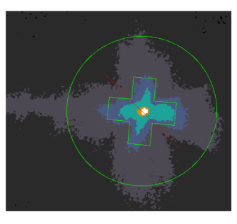
Figure 1.— An image from the XIS3 detector. The outer green circle is the source region with a radius of 100$\arcsec$, and the inner plus sign is the exclusion region which is used to correct pile-up effects. A readout streak can be seen on the figure.

Pile-up effects can be corrected using two methods. We use a concentric circle with a outer radius of 100$\arcsec$ as the source region. The coordinates of the region center are [$\alpha=18^{\rm h}39^{\rm m}56.201^{\rm s}$, $\delta=+5^{\circ}02^{\prime}04.58^{\prime\prime}$] for 408033010, [$\alpha=18^{\rm h}39^{\rm m}57.397^{\rm s}$, $\delta=+5^{\circ}02^{\prime}07.63^{\prime\prime}$] for 408033020 and [$\alpha=18^{\rm h}39^{\rm m}58.513^{\rm s}$, $\delta=+5^{\circ}02^{\prime}13.88^{\prime\prime}$] for 408033030. We then extracted a series of source spectra using an annulus with this outer radius, and varying the inner radius. The spectra were fitted in XSPEC, and by comparing the parameters of each spectrum, we found that the spectral shapes and fitting parameters began to settle when the radius of the inner exclusion region is 20$\arcsec$-30$\arcsec$ or larger, which is consistent with previous observations (Cackett et al., 2010). The other way to do pile-up correction is to use a script in the Interactive Spectral Interpretation System (ISIS) which provides a visual presentation of areas of pile-up in the clean event files . Based on the shapes of the areas with a high pile-up fraction ($\geq 0.05$), we found that the areas affected by pile-up were not circularly-distributed about but rather in the shape of a Maltese cross, which is the shape of the point spread function (PSF) for the telescope. This prompted the use of a plus-sign shaped exclusion region where each side of the polygon is 30$\arcsec$ in length with right angles (see Figure 1), instead of a circular region, to correct pile-up effects, as a circular exclusion region would filter more photons than actually needed. By comparing the pre-correction and post-correction spectra, we find that pile-up effects in this observation are fairly mild. Pile-up only caused slight differences between $\sim 1-4$ keV and above $\sim$ 7 keV in the spectra and did not affect the iron line profile.

The readout streak was present in the data from XIS3 (see Figure 1), and thus we did not combine the spectrum of XIS3 with that of the other front-illuminated detector, XIS0. We measured the counts taken from a region on the readout streak away from the source and found that on average $\sim$ 12% of events in the source region were caused by the readout streak in the full-window mode observation, implying $\sim$ 9% of affected photons in the 1/4-window mode observations. There is no significant variability between observations, and the XIS0, XIS1, and XIS3 spectra shown in the following were combined from the three observations.

The Hard X-ray Detector (HXD) was operated as well, in XIS nominal pointing mode, to collect high-energy photons of the source. We reduced the data following standard procedures. The background spectrum was produced by combining the non-X-ray background and the cosmic-X-ray background. As the background dominates above $\sim 26.0$ keV, we only use the data over the 15.0-26.0 keV energy range in the following analyses. For both XIS and HXD/PIN detectors, we used the ADDASCASPEC tool to combine the spectrum from each observation and obtained a total spectrum for each detector.

3. Data Analysis

3.1. Continuum Model

Serpens X-1 has been observed by different instruments at different times. There are several continuum models used in previous work, using different combinations of a disk blackbody, a blackbody and a power-law. A continuum model consisting of all three components was used most often, especially in broadband observations (2006 Suzaku observation: Cackett et al. 2008, 2010; 2013 NuSTAR observation: Miller et al. 2013). Continuum models including only a disk blackbody and a blackbody, or a blackbody and a power-law were used in previous observations as well, but only in observations with limited energy ranges (Bhattacharyya & Strohmayer, 2007; Chiang et al., 2016). We test the continuum models which successfully fit the archival data on our latest Suzaku observation.

We use the XIS data over the $1-10$ keV energy band, and the PIN spectrum over $15-26$ keV. The $1.45-2.5$ keV in the XIS spectra were ignored due to poor calibration around the Si and Au edges. An iron K emission line is detected in the spectra. In order not to bias continuum measurements, we first excluded the $5.0-7.5$ keV energy band (the iron line band) to test various continuum models in the initial fits. The Galactic absorption is modeled using TBABS in XSPEC; the accretion disk emission is modeled with DISKBB; the blackbody component which is likely caused by the boundary layer is accounted for using BBODY. We added a constant between the spectra (with that of the XIS0 spectrum frozen at 1.00) and linked all parameters except normalizations of DISKBB and BBODY. As there are mild spectral differences between the spectra of different XIS detectors, which are caused by calibration and different observation modes, the normalizations of DISKBB and BBODY components are free to vary for better results. The continuum model with all three components results in a $\chi^{2}/$d.o.f. of 2617/2323, and other models yield worse fits. The result is consistent with previous work using broadband X-ray data. We also test thermal Comptonization model using NTHCOMP (Zdziarski et al., 1996; Życki et al., 1999) in XSPEC, and it does not improve the fit. Since the TBABS*(DISKBB + BBODY + POWERLAW) continuum fits significantly better than other continuum models, we use it in all following analyses.

The best-fitting continuum model parameters are listed in Table 1. It can be seen that the neutral absorption column density $N_{\rm H}$ is higher than any value previously reported. The value of $N_{\rm H}$ reported in previous literature spans a wide range around $\sim$ (3-7.5)$\times 10^{21}$ cm^-2 (Cackett et al., 2008, 2010; Ng et al., 2010), and those obtained from Suzaku data are higher than the others. The highest $N_{\rm H}$ obtained from past work was $(7.5\pm 0.2)\times 10^{21}$ cm^-2 (1$\sigma$ uncertainty) obtained from pervious Suzaku observation (Cackett et al., 2010), while here $8.6^{+0.9}_{-0.7}\times 10^{21}$ cm^-2 is required to fit the data though the same absorption model is used. However, the abundance table used in Cackett et al. (2010) was Anders & Grevesse (1989). If we use the Anders & Grevesse (1989) abundance to fit the data, we obtain a $N_{\rm H}$ of $5.9^{+0.5}_{-0.3}\times 10^{21}$ cm^-2, which is lower than the value Cackett et al. (2010) reported and consistent with the historical range.

Note that the constant for the XIS3 is $1.25^{+0.04}_{-0.05}$. In previous section we found that the effect caused by the readout streak is $\sim$ 9%. The constant is still slightly higher than expected when the effect is accounted for due to unknown reason. The best-fitting values of remaining parameters shown in Table 1 are consistent with Cackett et al. (2008).

Table 1Best-fitting continuum model parameters.

Component	Parameter	XIS0	XIS1	XIS3	PIN
Constant		(1.00)	$0.97^{+0.02}_{-0.01}$	$1.25^{+0.04}_{-0.05}$	$0.65^{+0.03}_{-0.01}$
TBABS	$N_{\rm H}$ ($10^{22}$ cm-2)	$0.86^{+0.09}_{-0.07}$	$\cdots$	$\cdots$	$\cdots$
DISKBB	$kT_{\rm disk}$ (keV)	$1.36\pm 0.01$	$\cdots$	$\cdots$	$\cdots$
	$N_{\rm disk}$	$75\pm 4$	$71^{+5}_{-4}$	$79\pm 5$	$\cdots$
BBODY	$kT_{\rm bb}$ (keV)	$2.29^{+0.02}_{-0.03}$	$\cdots$	$\cdots$	$\cdots$
	$N_{\rm bb}$ ($10^{-2}$)	$3.6\pm 0.1$	$3.3\pm 0.1$	$3.3\pm 0.1$	$\cdots$
POWERLAW	$\Gamma$	$3.44^{+0.35}_{-0.33}$	$\cdots$	$\cdots$	$\cdots$
	$N_{\rm pow}$	$0.71^{+0.22}_{-0.16}$	$\cdots$	$\cdots$	$\cdots$

Note. — Parameters of the HXD/PIN spectrum are bound to those of the XIS0 spectrum. We use XIS data over the $1-10$ keV ($1.45-2.5$ keV excluded due to calibration issues), and PIN data over the $15-26$ keV energy bands. The $5-7.5$ keV (iron line energy band) was excluded here. The model results in a $\chi^{2}/$dof of 2617/2323.

3.2. Phenomenological Models

After fitting the continuum we reload the $5.0-7.5$ keV data and find that an iron emission line is clearly detected (see Fig. 2). In order to model the broadband X-ray spectrum with the iron line, we add a Gaussian component on top of the continuum model. We restrict the energy of the Gaussian line to be $6.4-6.97$ keV, which is the energy range that the Fe K$\alpha$ line can appear in the spectrum. The fitting results are listed in Table 2. The absorption column density is slightly higher than the value of continuum fitting. The photon index $\Gamma$ tends to be higher than those previously reported. Note that the Gaussian width $\sigma=0.74^{+0.04}_{-0.05}$ keV is higher than the broadest value in published literature ($\sigma$ = 0.61 keV, see Cackett et al. 2012), indicating the existence of a broad Fe K line. In addition, the equivalent width (EW) of the line $192^{+17}_{-15}$ eV is larger than values obtained from previous Serpens X-1 observations (Bhattacharyya & Strohmayer, 2007; Cackett et al., 2008, 2010; Chiang et al., 2016). These may imply that the Gaussian component is fitting part of the continuum, and whether the Fe K line is symmetric or not should be further investigated.

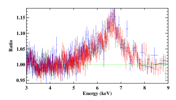
Figure 2.— Ratio of the data to the continuum model, showing the iron line profile. The continuum model was fit to the spectra with the $5.0-7.5$ keV region ignored. The XIS0, XIS1, and XIS3 data are presented by black, red and blue points, respectively. An broad iron emission line is clearly present in the spectrum.

Table 2Spectral fit parameters for the phenomenological models

Component	Parameter	Gaussian	DISKLINE	RELLINE
TBABS	$N_{\rm H}$ ($10^{22}$ cm-2)	$0.97^{+0.07}_{-0.08}$	$0.81^{+0.10}_{-0.05}$	$0.82^{+0.09}_{-0.06}$
DISKBB	$kT_{\rm disk}$ (keV)	$1.35^{+0.02}_{-0.01}$	$1.35\pm 0.01$	$1.35\pm 0.01$
	$N_{\rm disk}$	$78^{+5}_{-4}$	$75^{+13}_{-3}$	$75^{+4}_{-3}$
BBODY	$kT_{\rm bb}$ (keV)	$2.31\pm 0.01$	$2.27\pm 0.03$	$2.27\pm 0.03$
	$N_{\rm bb}$ ($10^{-2}$)	$3.6\pm 0.1$	$3.7\pm 0.1$	$3.7\pm 0.1$
POWERLAW	$\Gamma$	$3.87^{+0.23}_{-0.28}$	$3.22^{+0.42}_{-0.22}$	$3.24^{+0.41}_{-0.24}$
	$N_{\rm pow}$	$0.98^{+0.21}_{-0.19}$	$0.60^{+0.21}_{-0.11}$	$0.61^{+0.21}_{-0.11}$
Gaussian	$E_{\rm line}$	$6.4^{+0.02}$	$\cdots$	$\cdots$
	$\sigma$ (keV)	$0.74^{+0.04}_{-0.05}$	$\cdots$	$\cdots$
	$N_{\rm gau}$ ($10^{-3}$)	$10.0\pm 0.9$	$\cdots$	$\cdots$
LINE	$E_{\rm line}$ (keV)	$\cdots$	$6.97_{-0.02}$	$6.97_{-0.02}$
	$q$	$\cdots$	$4.24^{+0.24}_{-0.22}$	$4.22^{+0.25}_{-0.22}$
	$R_{\rm in}$ ($GM/c^{2}$)	$\cdots$	$8.1^{+0.4}_{-1.2}$	$8.1^{+0.5}_{-0.4}$
	$i$ (deg)	$\cdots$	$22\pm 1$	$23\pm 1$
	$N_{\rm line}$ ($10^{-3}$)	$\cdots$	$7.3^{+1.9}_{-0.5}$	$7.4^{+0.4}_{-0.6}$
EW (eV)		$192^{+17}_{-15}$	$147^{+9}_{-12}$	$146^{+8}_{-12}$
$\chi^{2}/$d.o.f.		3763/3352	3730/3350	3728/3350

Note. — For simplicity, we only present results of XIS1 (the $\chi^{2}/$d.o.f. is of the entire data set). The constant of each spectrum remains the same as those displayed in Table 1. Note that the emissivity index given by DISKLINE is $\beta$, which is equal to $-q$. We list $q$ here for easier comparison with other models.

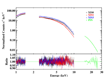
Figure 3.— The figure shows the XIS0 (black), XIS1 (red), XIS3 (blue) and PIN (green) spectra of Serpens X-1 fitted with the continuum plus a DISKLINE component. The lower panel is the data/model ratio, and it can be seen that the model fits the broadband spectrum well.

We replaced the Gaussian component with the DISKLINE model to fit the spectrum in order to examine if the line profile is better interpreted by relativistic effects, and to directly compare results with those previously published in the literature. It is generally believed that the Fe K line originates from an accretion disk around objects of strong gravity (i.e., black holes or neutron stars) and is shaped by a series of relativistic effects, including relativistic beaming and gravitational redshift, and appear to be broad and asymmetric. We froze the outer disk radius $R_{\rm out}$ at 1000 $R_{\rm G}$ in the fitting with other parameters of DISKLINE free to vary. The lower limit of the inner radius $R_{\rm in}$ in the model is 6 $R_{\rm G}$ and we restricted the inclination angle to vary between $5-80^{\circ}$. As shown in Table 2, the fit improves by $\Delta\chi^{2}=33$ with two lower degrees of freedom compared to the Gaussian model, and the model fits the data well (see Fig. 3). The F-test probability is $\sim 3.91\times 10^{-7}$, which is convincing that the DISKLINE model explains the data better. The EW of the Fe line obtained via the DISKLINE model is $147^{+9}_{-12}$ eV, which is also consistent with previous results (Cackett et al., 2008; Chiang et al., 2016).

The temperatures of the DISKBB and BBODY components are nearly identical in both models. Although the photon indices $\Gamma$ obtained from the models seem to be different, the fluxes of the powerlaw component are comparable. The differences between $\Gamma$ may be led by the mild differences in the blackbody temperatures. The DISKLINE model gives a slightly lower $N_{\rm H}$, indicating the parameter may be mildly model-dependent.

The parameters of the DISKLINE component are remarkably similar to previously reported numbers (Cackett et al., 2010; Chiang et al., 2016). We obtained an inner radius $R_{\rm in}=8.1^{+0.4}_{-1.2}$ $R_{\rm G}$, which is close to a number of previous results (Cackett et al., 2012; Miller et al., 2013; Chiang et al., 2016), and the line profile is similar as well (see Fig. 4).

We also replaced the DISKLINE model with the more modern RELLINE (Dauser et al., 2010, 2013) model (setting the spin parameter a* = 0), and find that a best-fitting inner radius of $8.1^{+0.5}_{-0.4}$ $R_{\rm G}$ (see Table 2), consistent with the DISKLINE fits. A low inclination angle $i$ $\sim 23\pm 1$ is required to fit the data, which is expected as low inclination has been reported in a series of past work (Cackett et al., 2010, 2012; Miller et al., 2013; Chiang et al., 2016). Optical observations of Serpens X-1 also point to a low inclination of less than 10^∘ (Cornelisse et al., 2013), which is in good agreement with the result of X-ray observations. Note that it is possible that the inner disk can be slightly mis-aligned with the binary orbit, for instance, see the case of GRO J1655$-$40 (Hjellming & Rupen, 1995; Greene et al., 2001).

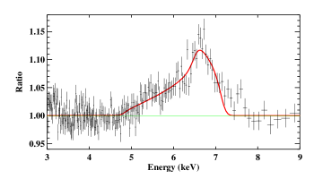
Figure 4.— The figure shows the iron line profile (XIS0 data only) fitted with the DISKLINE model.

3.3. Reflection Model

We learn from the tests of phenomenological models that the iron line is better explained by relativistic reflection. In order to confirm this scenario, we replace the DISKLINE component with a self-consistent reflection model which includes a broadband continuum and all emission lines originated from an illuminated accretion disk. Since the blackbody emission dominates the flux above 10 keV which implies the illuminating source is the boundary layer emission or stellar surface, we use the BBREFL (Ballantyne, 2004) grid, which calculates reflected emission from an accretion disk illuminated by a blackbody component, to model the reflection. We use the convolution kernel RELCONV (Dauser et al., 2010) to account for relativistic effects.

We list best-fitting parameters in Table 3. It can be seen that the fit has been improved by $\Delta\chi^{2}=99$ compared to the DISKLINE model. The decomposed model and data/model ratio can be found in Fig. 5. The values of the inner radius, inclination angle, and emissivity index are lower than those obtained from the DISKLINE model but consistent with the numbers reported in Miller et al. (2013). The reflection model gives a slightly higher $N_{\rm H}$ than those obtained from phenomenological models, but the values are roughly consistent within $3\sigma$. We again obtain a low inner radius $R_{\rm in}=6.7^{+0.8}_{-0.7}~{}R_{\rm G}$, and a low inclination angle $i=9^{+7}_{-4}$ degrees, implying measurements in previous work are robust.

Table 3Spectral fit parameters for the reflection model

Component	Parameter	BBREFL
TBABS	$N_{\rm H}$ ($10^{22}$ cm-2)	$1.00^{+0.07}_{-0.04}$
DISKBB	$kT_{\rm disk}$ (keV)	$1.29^{+0.01}_{-0.02}$
	$N_{\rm disk}$	$95^{+5}_{-6}$
BBODY	$kT_{\rm bb}$ (keV)	$2.33\pm 0.01$
	$N_{\rm bb}$ ($10^{-2}$)	$3.1^{+0.1}_{-0.2}$
POWERLAW	$\Gamma$	$4.14^{+0.24}_{-0.20}$
	$N_{\rm pow}$	$1.03^{+0.20}_{-0.12}$
RELCONV	$q$	$2.6^{+0.1}_{-0.2}$
	$R_{\rm in}$ ($GM/c^{2}$)	$6.7^{+0.8}_{-0.7}$
	$i$ (deg)	$9^{+7}_{-4}$
BBREFL	log $\xi$	$3.05^{+0.07}_{-0.06}$
	$N_{\rm bbrefl}$ ($10^{-26}$)	$1.5^{+0.2}_{-0.1}$
$\chi^{2}/$d.o.f.		3631/3350

Note. — For simplicity, we only present results of XIS1 (the $\chi^{2}/$d.o.f. is of the entire data set though). The constant of each spectrum remains the same as those displayed in Table 1.

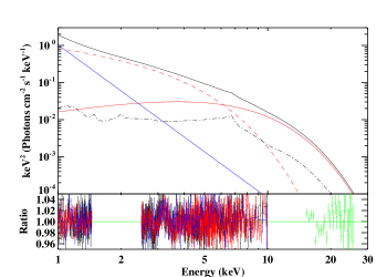
Figure 5.— The upper panel shows the decomposed best-fitting model. The red dash line represents the DISKBB component, the red solid line the BBODY component, the blue solid line the POWERLAW component, and the black dot dash line the blurred reflection continuum RELCONV$\times$BBREFL. The black sold line on top is the total model with all the components combined. The lower panel shows the data/model ratio, in which black, red, blue, and green data points stand for XIS0, XIS1, XIS3, and PIN data, respectively.

4. Discussion

Serpens X-1 has been observed by different missions in the past, and there are several measurements of the inner radius which can be found in the literature (Bhattacharyya & Strohmayer, 2007; Cackett et al., 2008, 2010; Miller et al., 2013; Chiang et al., 2016). As these archival observations were taken at different times, and possibly in different flux states, these offer the possibility to probe the evolution of the inner radius in Serpens X-1. We then check previous work to find fluxes and inner radii obtained from other observations, and compare these numbers with those of the present work. The $0.5-25.0$ keV absorption-corrected (unabsorbed) fluxes were converted into luminosities using a distance of 7.7 kpc (from X-ray burst properties, see e.g. Galloway et al. 2008). We list the $0.5-25.0$ keV luminosity and inner radius quoted from a number of previous observations (see Table 4). Note that these numbers were calculated using phenomenological models in which the DISKLINE model was used to model the iron line. In some references, measurements based on self-consistent relativistic reflection models are also listed, and we find most the results are consistent with phenomenological model calculations. In Cackett et al. (2010) and Miller et al. (2013) a continuum model which is the same with that of the present work was used, while in Chiang et al. (2016) a continuum model composed of a blackbody and a powerlaw components was used, but the authors reported that the line parameters are not continuum-dependent in that observation.

Table 4Luminosity and inner radius $R_{\rm in}$ of each previous Serpens X-1 observation

Observation	Luminosity (erg/s)	$L/L_{\rm Edd}$	Inner Radius $R_{\rm in}$ ($R_{\rm G}$)	Reference
Suzaku (2006)	$(8.5\pm 0.1)\times 10^{37}$	0.48	$8\pm 0.3$	Cackett et al. (2010)
XMM (2004, Obs ID 0084020401)	$(5.0\pm 0.1)\times 10^{37}$	0.28	$25\pm 8$	Cackett et al. (2010)
XMM (2004, Obs ID 0084020501)	$(3.6\pm 0.1)\times 10^{37}$	0.20	$14\pm 1$	Cackett et al. (2010)
XMM (2004, Obs ID 0084020601)	$(4.6\pm 0.1)\times 10^{37}$	0.26	$26\pm 8$	Cackett et al. (2010)
NuSTAR (2013)	$1.1\times 10^{38}$*	0.62	$10.6\pm 0.6$	Miller et al. (2013)
Chandra (2014)	$(6.7\pm 0.1)\times 10^{37}$	0.38	$7.7\pm 0.1$	Chiang et al. (2016)
Suzaku (2013-14)	$(7.1\pm 0.4)\times 10^{37}$	0.40	$8.1^{+0.4}_{-1.2}$	present work

Note. — The luminosity was calculated based on the $0.5-25.0$ keV absorption-corrected flux (measured using a phenomenological model) and a distance of 7.7 kpc. Luminosities quoted in Cackett et al. (2010) have much larger uncertainties due to including 25% of error on distance. In this work we only compare results of the same source, and uncertainties on distance were excluded. *Note that the flux of the NuSTAR observation was measured using the $0.5-40.0$ keV band. Since the high-energy tail of this source is weak, the $25.0-40.0$ keV energy band only contributes little flux.

It can be clearly seen that in Table 4 that the inner radius spans a range between $\sim 8-25$ $R_{\rm G}$ and the flux between $\sim(3-11)\times 10^{37}$ erg s^-1 ($\sim 0.2-0.6$ Eddington ratio $L/L_{\rm Edd}$ if assuming a mass of 1.4 $M_{\odot}$). Although some of the 2004 XMM-Newton observations give large inner radii of $\sim 25$ $R_{\rm G}$, these measurements are not well-constrained and analyses by Bhattacharyya & Strohmayer (2007) give smaller values. Note that the XMM data are the least reliable among these archival data due to short exposure and calibration issues of EPIC-PN timing mode data (see e.g. Walton et al. 2012), though the broad line does not seem to suffer from pile-up effects (Miller et al., 2010). In order to see how the inner radius evolves with the flux more clearly, we plot the results in Fig. 6 but exclude XMM results and only present well-constrained measurements for clarity.

The weighted mean of all inner radius measurements is $\sim 7.9~{}R_{\rm G}$, which is $\sim$16 km if assuming the neutron star mass to be 1.4 $M_{\odot}$. The measurement of the inner radius gives an upper limit of the size of the neutron star. It can be seen in Fig. 6 that more constrained measurements of the inner radius fall within a narrow range, implying that the accretion disk is not truncated at a large radius at fluxes $\gtrsim 0.4$ $L/L_{\rm Edd}$. Furthermore, from Fig. 6 it seems that the inner radius does not show a strong flux dependence. For a neutron star, the ISCO depends on the mass and radius of the neutron star and its equation of state. However, it should lie somewhere between $5-6$ $R_{\rm G}$ for reasonable parameters (Bhattacharyya, 2011). Our measured inner disk radius of $8~{}R_{\rm G}$, is therefore larger than the expected ISCO and stellar surface. The disk could therefore be truncated by either the stellar surface, the boundary layer between the disk and star, or the neutron star magnetic field.

If we assume that the magnetic field truncates the disk and therefore the magnetospheric radius is $7.9~{}R_{\rm G}$, we can estimate the magnetic field strength (see e.g., Illarionov & Sunyaev, 1975; Ibragimov & Poutanen, 2009; Cackett et al., 2009). Given that the unabsorbed $2-25$ keV flux of Serpens X-1 in this observation is $F_{\rm 2-25keV}=6.62\times 10^{-9}$ erg cm^-2 s^-1, we estimate the magnetic dipole moment $\mu=1.23\times 10^{26}$ G cm³ following the Equation (1) and assumptions in Cackett et al. (2009). This corresponds to a magnetic field strength at the poles of $B=2.5\times 10^{8}$ G (assuming a 10 km neutron star).

If the magnetic field is truncating the disk, then we would expect the inner disk radius to change with flux, since the magnetospheric radius depends on the mass accretion rate as $\dot{m}^{-2/7}$. To show the expected flux-dependence of the magnetospheric radius, we assume it is equal to 8 $R_{\rm G}$ at $L=6\times 10^{37}$ erg s^-1 and show the relation in Fig. 6 (see the blue dash line). The factor of $\sim$1.5 in flux that are covered all observations, would lead to an expected change by a factor of 0.9, with the highest flux observation having the smallest inner disk radius. This is not what we see here, with the largest radius being at the highest flux. This may be more easily explained if the disk is truncated by the boundary layer, with the boundary increasing in size with mass accretion rate, as expected from theoretical considerations (Popham & Sunyaev, 2001). We also show the dependence of the boundary layer radius with flux in Fig. 6 (red dash line) using equation 25 of Popham & Sunyaev (2001), and relating $\dot{M}$ to $L$ through $L_{\rm acc}=GM\dot{M}/R_{*}=1.17\times 10^{37}~{}(\dot{M}/10^{-9}~{}M_{\odot}$ yr^-1) erg s^-1, where $R_{*}$ is the neutron star radius assumed to be 10 km and the neutron star mass $M=1.4~{}M_{\odot}$ (see the red dash line in Fig. 6). The increase in inner disk radius at the highest mass accretion rate is similar to the size of the boundary layer predicted by Popham & Sunyaev (2001). The Popham & Sunyaev boundary layer model, however, assumes a nonmagnetic neutron star and the addition of a magnetic field will presumably change the boundary layer structure somewhat.

Steiner et al. (2010) found values of the inner radius of the black hole binary LMC X-3 to be consistent within $4-6$% across eight X-ray missions, implying the inner radius is stable over different flux states. In neutron star LMXBs the evolution of inner radius has also been studied. Lin et al. (2010) found that the accretion disk of the neutron star system 4U 1705$-$44 is close to the neutron star during soft states based on the broad iron line. In hard states of 4U 1705$-$44, whether the accretion disk is truncated is however debated. D’Aì et al. (2010) suggested the accretion disk to be truncated, while Di Salvo et al. (2015) indicated that it is not truncated at large radii, down to $\sim$ 3% of Eddington luminosity. 4U 1636$-$53 also shows no clear evolution in inner disk radius around the color-color diagram (Sanna et al., 2014). Serpens X-1 has only been observed during soft states, and the inner radius evolution during hard states remains unclear. But in soft states the inner radius is roughly constant over fluxes changing by a factor of around 1.5, and the accretion disk stays close in at least down to $\sim$0.4$L/L_{\rm Edd}$.

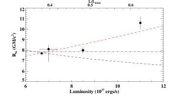
Figure 6.— The figure is the visualization of Table 4 shows the inner radii measured in previous literature in different flux states. We assume a mass of 1.4$M_{\odot}$ to convert the luminosity into the Eddington ratio $L/L_{\rm Edd}$. The black dash dot line marks the weighted mean of the inner radius measurements; the blue dash line shows the prediction of the magnetosphere radius; the red dash line presents the prediction of the boundary layer model.

5. Conclusion

We present detailed spectral analysis of the latest, longest Suzaku observation of the neutron star LMXB Serpens X-1 in this work. The continuum is best explained by the combination of a disk blackbody component, a single-temperature blackbody component and a powerlaw component, which is consistent with the results of previous broadband observations. We find that the relativistic reflection scenario is the better interpretation of the iron line profile shown in this observation. The line parameters obtained are consistent with a number of previous work. By comparing the inner radius obtained from different observations taken at different flux states, we find no strong evidence that the inner radius evolves with flux, with the inner radius staying at $\sim$8 $R_{\rm G}$. The observation with the highest flux shows the largest inner disk radius, implying that a boundary layer, rather than the stellar magnetic field, truncates the disk outside the ISCO. Results of current data indicate that the inner radius stays unchanged at soft states. To further confirm if this stands true for hard states, multiple observations at different times on the same source should be performed to cover a wider range of flux states.

References

- Anders & Grevesse (1989) Anders, E., & Grevesse, N. 1989, Geochim. Cosmochim. Acta, 53, 197
- Arnaud (1996) Arnaud, K. A. 1996, in Astronomical Society of the Pacific Conference Series, Vol. 101, Astronomical Data Analysis Software and Systems V, ed. G. H. Jacoby & J. Barnes, 17
- Ballantyne (2004) Ballantyne, D. R. 2004, MNRAS, 351, 57
- Barret (2001) Barret, D. 2001, Advances in Space Research, 28, 307
- Bhattacharyya (2011) Bhattacharyya, S. 2011, MNRAS, 415, 3247
- Bhattacharyya & Strohmayer (2007) Bhattacharyya, S., & Strohmayer, T. E. 2007, ApJ, 664, L103
- Cackett et al. (2009) Cackett, E. M., Altamirano, D., Patruno, A., et al. 2009, ApJ, 694, L21
- Cackett et al. (2012) Cackett, E. M., Miller, J. M., Reis, R. C., Fabian, A. C., & Barret, D. 2012, ApJ, 755, 27
- Cackett et al. (2008) Cackett, E. M., Miller, J. M., Bhattacharyya, S., et al. 2008, ApJ, 674, 415
- Cackett et al. (2010) Cackett, E. M., Miller, J. M., Ballantyne, D. R., et al. 2010, ApJ, 720, 205
- Chiang et al. (2016) Chiang, C.-Y., Cackett, E. M., Miller, J. M., et al. 2016, ApJ, 821, 105
- Cornelisse et al. (2013) Cornelisse, R., Casares, J., Charles, P. A., & Steeghs, D. 2013, MNRAS, 432, 1361
- D’Aì et al. (2010) D’Aì, A., di Salvo, T., Ballantyne, D., et al. 2010, A&A, 516, A36
- Dauser et al. (2013) Dauser, T., Garcia, J., Wilms, J., et al. 2013, MNRAS, 430, 1694
- Dauser et al. (2010) Dauser, T., Wilms, J., Reynolds, C. S., & Brenneman, L. W. 2010, MNRAS, 409, 1534
- Degenaar et al. (2015) Degenaar, N., Miller, J. M., Chakrabarty, D., et al. 2015, MNRAS, 451, L85
- Di Salvo et al. (2015) Di Salvo, T., Iaria, R., Matranga, M., et al. 2015, MNRAS, 449, 2794
- Done et al. (2007) Done, C., Gierliński, M., & Kubota, A. 2007, A&A Rev., 15, 1
- Fabian et al. (2000) Fabian, A. C., Iwasawa, K., Reynolds, C. S., & Young, A. J. 2000, PASP, 112, 1145
- Fabian et al. (1989) Fabian, A. C., Rees, M. J., Stella, L., & White, N. E. 1989, MNRAS, 238, 729
- Fabian & Ross (2010) Fabian, A. C., & Ross, R. R. 2010, Space Sci. Rev., 157, 167
- Galloway et al. (2008) Galloway, D. K., Muno, M. P., Hartman, J. M., Psaltis, D., & Chakrabarty, D. 2008, ApJS, 179, 360
- Greene et al. (2001) Greene, J., Bailyn, C. D., & Orosz, J. A. 2001, ApJ, 554, 1290
- Guilbert & Rees (1988) Guilbert, P. W., & Rees, M. J. 1988, MNRAS, 233, 475
- Hasinger & van der Klis (1989) Hasinger, G., & van der Klis, M. 1989, A&A, 225, 79
- Hjellming & Rupen (1995) Hjellming, R. M., & Rupen, M. P. 1995, Nature, 375, 464
- Homan et al. (2010) Homan, J., van der Klis, M., Fridriksson, J. K., et al. 2010, ApJ, 719, 201
- Ibragimov & Poutanen (2009) Ibragimov, A., & Poutanen, J. 2009, MNRAS, 400, 492
- Illarionov & Sunyaev (1975) Illarionov, A. F., & Sunyaev, R. A. 1975, A&A, 39, 185
- Lightman & White (1988) Lightman, A. P., & White, T. R. 1988, ApJ, 335, 57
- Lin et al. (2007) Lin, D., Remillard, R. A., & Homan, J. 2007, ApJ, 667, 1073
- Lin et al. (2009) —. 2009, ApJ, 696, 1257
- Lin et al. (2010) —. 2010, ApJ, 719, 1350
- Ludlam et al. (2016) Ludlam, R. M., Miller, J. M., Cackett, E. M., et al. 2016, ApJ, 824, 37
- Miller (2007) Miller, J. M. 2007, ARA&A, 45, 441
- Miller et al. (2006) Miller, J. M., Homan, J., & Miniutti, G. 2006, ApJ, 652, L113
- Miller et al. (2010) Miller, J. M., D’Aì, A., Bautz, M. W., et al. 2010, ApJ, 724, 1441
- Miller et al. (2013) Miller, J. M., Parker, M. L., Fuerst, F., et al. 2013, ApJ, 779, L2
- Narayan & Yi (1995) Narayan, R., & Yi, I. 1995, ApJ, 452, 710
- Ng et al. (2010) Ng, C., Díaz Trigo, M., Cadolle Bel, M., & Migliari, S. 2010, A&A, 522, A96
- Pandel et al. (2008) Pandel, D., Kaaret, P., & Corbel, S. 2008, ApJ, 688, 1288
- Popham & Sunyaev (2001) Popham, R., & Sunyaev, R. 2001, ApJ, 547, 355
- Reis et al. (2010) Reis, R. C., Fabian, A. C., & Miller, J. M. 2010, MNRAS, 402, 836
- Reis et al. (2009) Reis, R. C., Fabian, A. C., Ross, R. R., & Miller, J. M. 2009, MNRAS, 395, 1257
- Sanna et al. (2013) Sanna, A., Hiemstra, B., Méndez, M., et al. 2013, MNRAS, 432, 1144
- Sanna et al. (2014) Sanna, A., Méndez, M., Altamirano, D., et al. 2014, MNRAS, 440, 3275
- Shakura & Sunyaev (1973) Shakura, N. I., & Sunyaev, R. A. 1973, A&A, 24, 337
- Shapiro et al. (1976) Shapiro, S. L., Lightman, A. P., & Eardley, D. M. 1976, ApJ, 204, 187
- Steiner et al. (2010) Steiner, J. F., McClintock, J. E., Remillard, R. A., et al. 2010, ApJ, 718, L117
- Tomsick et al. (2009) Tomsick, J. A., Yamaoka, K., Corbel, S., et al. 2009, ApJ, 707, L87
- Walton et al. (2012) Walton, D. J., Reis, R. C., Cackett, E. M., Fabian, A. C., & Miller, J. M. 2012, MNRAS, 422, 2510
- Wilms et al. (2000) Wilms, J., Allen, A., & McCray, R. 2000, ApJ, 542, 914
- Zdziarski et al. (1996) Zdziarski, A. A., Johnson, W. N., & Magdziarz, P. 1996, MNRAS, 283, 193
- Życki et al. (1999) Życki, P. T., Done, C., & Smith, D. A. 1999, MNRAS, 309, 561