Accelerated first-order methods for large-scale convex minimization

Abstract

This paper discusses several (sub)gradient methods attaining the optimal complexity for smooth problems with Lipschitz continuous gradients, nonsmooth problems with bounded variation of subgradients, weakly smooth problems with Hölder continuous gradients. The proposed schemes are optimal for smooth strongly convex problems with Lipschitz continuous gradients and optimal up to a logarithmic factor for nonsmooth problems with bounded variation of subgradients. More specifically, we propose two estimation sequences of the objective and give two iterative schemes for each of them. In both cases, the first scheme requires the smoothness parameter and the Hölder constant, while the second scheme is parameter-free (except for the strong convexity parameter which we set zero if it is not available) at the price of applying a nonmonotone backtracking line search. A complexity analysis for all the proposed schemes is given. Numerical results for some applications in sparse optimization and machine learning are reported, which confirm the theoretical foundations.

1 Introduction

Let $V$ be a finite-dimensional linear vector space with the dual space $V^{*}$ as the space of all linear function on $V$. We assume $f:V\rightarrow\overline{\mathbb{R}}:=\mathbb{R}\cup\{+\infty\}$ is a proper, $\mu_{f}$-strongly convex ($\mu_{f}>0$ for strongly convex case and $\mu_{f}=0$ for convex case), and lower semicontinuous function satisfying

$$\|\nabla f(x)-\nabla f(y)\|_{*}\leq L_{\nu}\|x-y\|^{\nu}~{}~{}~{}\forall~{}x,y\in V,$$ (1)

where $\nabla f(x)$ denotes the gradient of $f$ at $x$ for $\nu\in(0,1]$ or any subgradient of $f$ at $x$ ($\nabla f(x)\in\partial f(x)$) for $v=0$. Let the function $\psi:V\rightarrow\overline{\mathbb{R}}$ be simple, proper, $\mu_{p}$-strongly convex ($\mu_{p}\geq 0$), and lower semicontinuous function. We consider the structured convex minimization problem

$$\begin{array}[]{ll}\min&~{}h(x):=f(x)+\psi(x)\\ \mathrm{s.t.}&~{}x\in C,\end{array}$$ (2)

where $C$ is a simple, nonempty, closed, and convex set. By (1), we have $f\in\mathcal{C}_{\mu_{f},L_{\nu}}^{1,\nu}(V)$, i.e., $f$ can be smooth with Lipschitz continuous gradients ($\nu=1$), weakly smooth problems with Hölder continuous gradients ($\nu\in{]0,1[}$), or nonsmooth with bounded variation of subgradients ($\nu=0$). Hence the objective $h$ is $\mu$-strongly convex with $\mu:=\mu_{f}+\mu_{p}\geq 0$. We assume that the first-order black-box oracle of the objective $h$ is available.

1.1 Motivation & history

Over the past few decades, due to the dramatic increase in the size of data for many applications, first-order methods have been received much attention thanks to their simple structures and low memory requirements. The efficiency of first-order methods can be poor (a large number of function values and subgradients is needed) for solving the general convex problems if the structure of the problem is not available. As a result, to develop practically appealing schemes, it is necessary to make an additional restriction on problem classes. In particular, developing efficient methods for solving large-scale convex optimization problems is possible if the underlying objective has a suitable structure and the domain is simple enough. Convexity and level of smoothness are two important factors playing key roles in construction of efficient schemes for such structured optimization problems.

Let $x^{*}$ be an optimizer of (2) and $x_{k}$ be an approximate solution given by a first-order method. We call $x_{k}$ an $\varepsilon$-solution of (2) if $h(x_{k})-h(x^{*})\leq\varepsilon$, for a prescribed accuracy parameter $\varepsilon>0$. In 1983, Nemirovski & Yudin in NemY derived optimal worst-case complexities for first-order methods to achieve an $\varepsilon$-solution for several classes of convex problems (see Table 1). If a first-order scheme attains the worst-case complexity of a class of problems, it is called optimal. A special feature of these methods is that the corresponding complexity does not depend explicitly on the problem dimension. From practical point of view, studying the effect of an uniform boundedness of the complexity is very attractive and such methods are highly recommended when the prescribed accuracy $\varepsilon$ is not too small, whereas the dimension of problem is considerably large.

Table 1: List of the best known complexities of first-order methods for several classes of problems with respect to levels of smoothness and convexity (cf. NemN; NemY; NesB)

Problem’s class	Convex problems	Strongly convex problems
Smooth problems ($\nu=1$)	$\mathcal{O}(\varepsilon^{-1/2})$	$\mathcal{O}(\ln(1/\varepsilon))$
Weakly smooth problems ($\nu\in{]0,1[}$)	$\mathcal{O}(\varepsilon^{-2/(1+3\nu)})$	$\leq\mathcal{O}(\varepsilon^{-{(1-\nu)}/(1+3\nu)})\ln\left(1/\varepsilon^{{(3+\nu)}/(1+3\nu)}\right)$
Nonsmooth problems ($\nu=0$)	$\mathcal{O}(\varepsilon^{-2})$	$\mathcal{O}(1/\varepsilon)$

In NemY, it was proved that subgradient, subgradient projection, and mirror descent methods possess the optimal complexity $\mathcal{O}(\varepsilon^{-2})$ for Lipschitz continuous nonsmooth problems, where the mirror decent method is a generalization of the subgradient projection method, cf. BecT1. In 1983, the pioneering optimal method by Nesterov Nes83 was introduced for smooth problems with Lipschitz continuous gradients. He later in NesB proposed some more gradient methods for this class of problems. Nesterov in NesC proposed a gradient-type method for minimizing the composite problem (2) with the complexity $\mathcal{O}(\varepsilon^{-1/2})$, where $f$ has Lipschitz continuous gradients and $\psi$ is a simple convex function. Since 1983 many researchers have developed the idea of optimal schemes, see, e.g., Auslander & Teboulle AusT, Baes Bae, Baes & Bürgisser BaeB, Beck & Teboulle BecT2, Chen et al. CheLO1; CheLO2, Gonzaga et al. GonK; GonKR, Juditsky & Nesterov JudN, Lan LanS; LanB, Lan et al. LanLM, Nesterov NesB, Neumaier NeuO and Tseng Tse. Computational experiments for problems of the form (2) have shown that Nesterov-type optimal first-order methods are substantially superior to the gradient descent and subgradient methods, cf. Ahookhosh Aho and Becker et al. BecCG. Nesterov also in NesS; NesE proposed some smoothing methods for a class of structured nonsmooth problems attaining the complexity $\mathcal{O}(\varepsilon^{-1/2})$.

In 1985, the first optimal method for weakly smooth objectives with Hölder continuous gradients was given by Nemirovski & Nesterov NemN; however, to implement this scheme, one needs to know about $\nu$, $L_{\nu}$, an estimate of the distance of starting point to the optimizer, and the total number of iterations, which makes the algorithm to some extent impractical. Lan LanB proposed an accelerated bundle-level method attaining the optimal complexity for all the convex classes considered. This scheme does not need to know about the global parameters such as Lipschitz or Hölder constants and the level of smoothness parameter $\nu$; on the other hand, as the scheme proceeds, the associated auxiliary problem becomes more difficult to solve, i.e., even the limited memory version of this scheme involves solving a computationally costly auxiliary problems. Devolder et al. DevGN; DevGN1 also proposed some first-order methods for minimization of objectives with Hölder continuous gradients in inexact oracle. The proposed fast gradient method attains the optimal complexities for convex problems; however, for implementation it needs to know about $\nu$, $L_{\nu}$, an estimate of the distance of starting point to the optimizer, and the total number of iterations. Recently, Nesterov NesU proposed a so-called universal gradient method for convex problem classes attaining the optimal complexities and requiring no global parameters at the price of applying a backtracking line search. More recently, Nesterov proposed a conditional gradient method involving a simple subproblem, which possesses the complexity $\mathcal{O}(\varepsilon^{-1/2\nu})$. Moreover, Ghadimi Gha and Ghadimi et al. GhaLZ developed some first-order methods for unconstrained nonconvex problems of the form (2) where $f$ is an arbitrary nonconvex function.

1.2 Contribution

This paper describes four accelerated (sub)gradient algorithms (ASGA) attaining optimal complexities for solving several classes of convex optimization problems with high-dimensional data (see Table 1).

We firstly construct an estimation sequence using available local or global information of $f$ and then give two iterative schemes for solving (2). The first scheme (ASGA-1) requires the level of smoothness $\nu$ and the Hölder constant $L_{\nu}$. Afterwards, we develop a parameter-free variant of this scheme (ASGA-2) that is not requiring $\nu$ and $L_{\nu}$ at the price of applying a backtracking line search. Apart from an initial point $x_{0}$ and the strong convexity parameter $\mu$ ($\mu=0$ if it is not available), ASGA-2 requires no more parameters. We here emphasize that parameter-free methods are useful for black-box optimization when no information about $\nu$ and $L_{\nu}$ is available.

We secondly generalize the estimation sequence of Nesterov NesU, by adding a quadratic term including the strong convexity information of $h$ and develop two (sub)gradient methods. The first one (ASGA-3) needs the smoothness parameters $\nu$ and $L_{\nu}$; on the other hand, the second one (ASGA-4) is parameter-free at the price of carrying out a backtracking line search.

The estimation sequence used in ASGA-1 and ASGA-2 shares some similarities with the estimation sequence used in ASGA-3 and ASGA-4; however, the iteration sequences used in construction of them are different. Whereas ASGA-1 requires a single solution of an auxiliary problem, ASGA-3 needs to solve two auxiliary problems. ASGA-2 requires at least a single solution of an auxiliary problem; in contrast, ASGA-4 needs to solve at least two auxiliary problems. As apposed to ASGA-1 and ASGA-3, the schemes NESUN, ASGA-2, and ASGA-4 are parameter-free (except for strong convexity parameter $\mu$ which we set $\mu=0$ if it is not available) by applying a backtracking line search. NESUN treats strongly convex problems by the same way as convex ones; on the other hand, ASGA-1, ASGA-2, ASGA-3, and ASGA-4 possess a much better complexity for strongly convex problems. It is worth mentioning that, for $\mu=0$, ASGA-4 almost reduces to NESUN except for some parameters.

Apart from some constants, ASGA-1, ASGA-2, ASGA-3, and ASGA-4 possess the same complexity for finding an $\varepsilon$-solution of the problem (2), i.e.,

$$\mathcal{O}\left(\mu^{-\frac{1+\nu}{1+3\nu}}L_{\nu}^{\frac{2}{1+3\nu}}\varepsilon^{-\frac{1-\nu}{1+3\nu}}\ln(\varepsilon^{-\frac{2}{1+\nu}})\right),$$

for $\mu>0$, and

$$\mathcal{O}\left(\varepsilon^{-\frac{2}{1+3\nu}}\right),$$

for $\mu=0$. Therefore, ASGA-1, ASGA-2, ASGA-3, and ASGA-4 are optimal for smooth, weakly smooth, and nonsmooth convex objectives. On the other hand, they are optimal for smooth strongly convex problems and optimal up to a logarithmic factor for nonsmooth strongly convex objectives. For weakly smooth strongly convex problems, they attain a complexity better than the known complexity for weakly smooth convex problems.

We finally study the solution of auxiliary problems appearing in ASGA-1, ASGA-2, ASGA-3, and ASGA-4. The considered auxiliary problems are strongly convex; however, finding their unique solutions efficiently is highly related to the structure involved in $\psi$ and $C$. It is shown that these auxiliary problems can be solved either in a closed form or by a simple iterative scheme for several functions $\psi$ and domain $C$ appearing in applications. Some computational experiments show that the performance of ASGA-2, ASGA-4, and NESUN are sensitive to large regularization parameters and small $\varepsilon>0$ (because of the associated line searches); whereas, ASGA-1 and ASGA-3 are less sensitive. In addition, there are many applications with available smoothness parameters $\nu$ and $L_{\nu}$ motivating the quest for designing ASGA-1 and ASGA-3. It is worth noting that the proposed schemes are able to handle sum of nonsmooth functions, where they behave much better than the traditional subgradient methods in spite of attaining the same complexity (see Section 5.3). Some encouraging numerical results are reported confirming the achieved theoretical foundations.

The remainder of the paper is organized as follows. In the next section we give two single-subproblem accelerated (sub)gradient schemes with their complexity analysis. In Section 3 we generalize the estimation sequence of Nesterov NesU and propose two double-subproblem accelerated (sub)gradient schemes and the related complexity analysis. In Section 4 we discuss the solution of the auxiliary problems appearing in the proposed methods. In Section 5 we reports some numerical experiments and comparisons showing the performance of the proposed methods. Finally, some conclusions are delivered in Section 6.

1.3 Preliminaries & notation

Let the primal space $V$ be endowed with a norm $\|\cdot\|$, and let the associated dual norm be defined by

$$\|s\|_{*}=\max_{x\in V}\{\langle s,x\rangle~{}|~{}\|x\|\leq 1\},$$

where $\langle s,x\rangle$ denotes the value of the linear function $s\in V^{*}$ at $x\in V$. If $V=\mathbb{R}^{n}$, then, for $1\leq p\leq\infty$,

$$\|x\|_{p}=\left(\sum_{i=1}^{n}|x_{i}|^{p}\right)^{1/p}.$$

For a function $\widetilde{f}:V\rightarrow\overline{\mathbb{R}}=\mathbb{R}\cup\{\pm\infty\}$, $\mathrm{dom}~{}\widetilde{f}=\{x\in V~{}|~{}\widetilde{f}(x)<+\infty\}$ denotes its effective domain, and $\widetilde{f}$ is called proper if $\mathrm{dom}~{}\widetilde{f}\neq\emptyset$ and $\widetilde{f}(x)>-\infty$ for all $x\in V$. Let $C$ be a subset of $V$. In particular, if $C$ is a box, we denote it by $\mathbf{x}=[\underline{x},\overline{x}]$, where in which $\underline{x}$ and $\overline{x}$ are the vectors of lower and upper bounds on the components of x, respectively. The vector $\nabla\widetilde{f}(x)\in V^{*}$ is called a subgradient of $\widetilde{f}$ at $x$ if $\widetilde{f}(x)\in\mathbb{R}$ and

$$\widetilde{f}(y)\geq\widetilde{f}(x)+\langle\nabla\widetilde{f}(x),y-x\rangle~{}~{}~{}\forall y\in V.$$

The set of all subgradients is called the subdifferential of $\widetilde{f}$ at $x$, which is denoted by $\partial\widetilde{f}(x)$.

If $\widetilde{f}$ is nonsmooth and convex, then Fermat-type optimality condition for the nonsmooth convex optimization problem

$$\begin{array}[]{ll}\min&~{}\widetilde{f}(x)\\ \mathrm{s.t.}&~{}x\in C\end{array}$$

is given by

$$0\in\partial\widetilde{f}(x)+N_{C}(x),$$ (3)

where $N_{C}(x)$ is the normal cone of $C$ at $x$, i.e.,

$$N_{C}(x):=\{p\in V\mid\langle p,x-z\rangle\geq 0~{}~{}\forall z\in C\}.$$ (4)

For $C\subseteq V$ and $y\in V$, the orthogonal projection is given by

$$\mathrm{P}_{C}(y):=\mathop{\rm argmin}_{x\in C}~{}\frac{1}{2}\|x-y\|^{2}.$$ (5)

The proximal-like operator $\mathrm{prox}_{\lambda\widetilde{f}}^{C}(y)$ is the unique optimizer of the optimization problem

$$\mathrm{prox}_{\lambda\widetilde{f}}^{C}(y):=\mathop{\rm argmin}_{x\in C}~{}\frac{1}{2}\|x-y\|_{2}^{2}+\lambda\widetilde{f}(x),$$ (6)

where $\lambda>0$. From (3), the first-order optimality condition for the problem (6) is given by

$$0\in x-y+\lambda\partial\widetilde{f}(x)+N_{C}(x).$$ (7)

If $C=V$, then (7) is simplified to

$$0\in x-y+\lambda\partial\widetilde{f}(x),$$ (8)

giving the classical proximity operator.

Let $\omega:V\rightarrow\mathbb{R}$ be a differentiable $1$-strongly convex function, i.e.,

$$\omega(y)\geq\omega(x)+\langle\nabla\omega(x),y-x\rangle+\frac{1}{2}\|y-x\|^{2}.$$ (9)

It is assumed that $\omega(x)$ attains its unique minimizer at $x_{0}$ and $\omega(x_{0})=0$. The function $\omega$ satisfied these conditions is called a prox-function. The corresponding Bregman distance is defined by

$$B_{\omega}(x,y):=\omega(x)-\omega(y)-\langle\nabla\omega(y),x-y\rangle,$$ (10)

where, from (9), it is straightforward to show

$$B_{\omega}(x,y)\geq\frac{1}{2}\|x-y\|^{2}.$$ (11)

2 Single-subproblem accelerated (sub)gradient methods

In this section we first give two schemes for solving structured problems of the form (2) attaining the optimal complexity for smooth, nonsmooth, weakly smooth, and smooth strongly problems. These schemes are optimal up to a logarithmic factor for nonsmooth strongly convex objectives. We then investigate the complexity analysis of these schemes.

To guarantee the existence of a solution of a problem of the form (2), we assume:

(H1) The upper level set $N_{h}(x_{0}):=\{x\in C\mid h(x)\leq h(x_{0})\}$ is bounded, for a starting point $x_{0}\in C$.

Since $h$ is convex and $N_{h}(x_{0})$ is closed, (H1) implies that $N_{h}(x_{0})$ is convex and compact. It therefore follows from the continuity and properness of the objective function $h$ that it attains its global minimizer on $N_{h}(x_{0})$. This guarantees that there is at least one minimizer $x^{*}$.

Motivated by Nesterov NesU, we define

$$L_{\nu}:=\sup_{x,y\in C,~{}x\neq y}\frac{\|\nabla f(x)-\nabla f(y)\|}{\|x-y\|^{\nu}},$$ (12)

for the level of smoothness parameter $\nu\in[0,1]$. If $L_{\nu}<+\infty$, then (12) implies that (1) holds resulting to

$$f(x)\leq f(y)+\langle\nabla f(y),x-y\rangle+\frac{L_{\nu}}{1+\nu}\|x-y\|^{1+\nu}~{}~{}~{}\forall x,y\in C.$$ (13)

The following proposition is crucial for constructing our accelerated (sub)gradient schemes, where for the sake of simplicity for $\nu=1$, we suppose $0^{0}=1$ in which $\widetilde{L}=L_{\nu}$ is a Lipschitz constant.

Proposition1

(NesU, Lemma 2) Let function $f$ satisfies the condition (1). Then, for $\delta>0$ and

$$\widehat{L}\geq\left(\frac{1-\nu}{\delta(1+\nu)}\right)^{\frac{1-\nu}{1+\nu}}L_{\nu}^{\frac{2}{1+\nu}}:=\widetilde{L},$$ (14)

we have

$$f(x)\leq f(y)+\langle\nabla f(y),x-y\rangle+\frac{1}{2}\widehat{L}\|x-y\|^{2}+\frac{\delta}{2}~{}~{}~{}x,y\in C.$$ (15)

The idea is to generate a sequence of estimation functions $\{\phi_{k}(x)\}_{k\geq 0}$ of $h$ in such a way that, at each iteration $k\geq 0$, the inequality

$$S_{k}\left(h(x_{k})-\frac{\varepsilon}{2}\right)\leq\phi_{k}^{*}:=\min_{x\in C}~{}\phi_{k}(x)$$ (16)

holds for $x_{k}\in V$, where $S_{k}$ is a scaling parameter. We consider the sequence of scaling parameters $\{S_{k}\}_{k\geq 0}$, which is generated by

$$S_{k}:=S_{k-1}+s_{k},$$ (17)

where $S_{0}=0$ and $s_{k}>0$. We consider the estimation sequence

$$\begin{array}[]{l}\phi_{k+1}(x):=\left\{\begin{array}[]{ll}B_{\omega}(x,x_{0})&~{}~{}\mathrm{if}~{}k=0,\vspace{3mm}\\ \phi_{k}(x)+s_{k+1}\left[q_{k+1}(x,y_{k})+\psi(x)\right]&~{}~{}\mathrm{if}~{}k\in\mathbb{N},\\ \end{array}\right.\vspace{3mm}\\ \displaystyle q_{k+1}(x,y_{k}):=f(y_{k})+\langle\nabla f(y_{k}),x-y_{k}\rangle+\frac{\mu_{f}}{2}\|x-y_{k}\|^{2}.\end{array}$$ (18)

Let us define $\{z_{k}\}_{k\geq 0}$ as the sequence of minimizers of the estimation sequence $\{\phi_{k}\}_{k\geq 0}$, i.e.,

$$z_{k+1}:=\displaystyle\mathop{\rm argmin}_{x\in C}~{}\phi_{k+1}(x).$$ (19)

The next result is crucial for the complexity analysis and for providing a stopping criterion for schemes will be presented in Section 2.1.

Proposition2

Let the sequence $\{\phi_{k}\}_{k\geq 0}$ be generated by (18). Then

$$\phi_{k}(x)\leq S_{k}~{}h(x)+B_{\omega}(x,x_{0})~{}~{}~{}\forall k\geq 0.$$ (20)

If in addition (16) holds, then

$$h(x_{k})-h(x^{*})\leq\frac{B_{\omega}(x^{*},x_{0})}{S_{k}}+\frac{\varepsilon}{2}.$$ (21)

Proof

The proof is given by induction on $k$. Since $S_{0}=0$ and $\phi_{0}(x)=B_{\omega}(x,x_{0})$, the result is valid for $k=0$. We assume it is true for $k$ and prove it for $k+1$. By this assumption and (18), we get

$$\begin{split}\phi_{k+1}(x)&=\phi_{k}(x)+s_{k+1}\left(f(y_{k})+\langle\nabla f(y_{k}),x-y_{k}\rangle+\frac{\mu_{f}}{2}\|x-y_{k}\|^{2}+\psi(x)\right)\\ &\leq S_{k}h(x)+B_{\omega}(x,x_{0})+s_{k+1}\left(f(y_{k})+\langle\nabla f(y_{k}),x-y_{k}\rangle+\frac{\mu_{f}}{2}\|x-y_{k}\|^{2}+\psi(x)\right)\\ &\leq S_{k}h(x)+B_{\omega}(x,x_{0})+s_{k+1}h(x)=S_{k+1}h(x)+B_{\omega}(x,x_{0}).\end{split}$$

From (16) and (20), we obtain

$$h(x_{k})\leq\frac{\varepsilon}{2}+\frac{1}{S_{k}}\phi_{k}^{*}\leq\frac{\varepsilon}{2}+\frac{1}{S_{k}}\min_{x\in C}(S_{k}~{}h(x)+B_{\omega}(x,x_{0}))=\frac{\varepsilon}{2}+h(x^{*})+\frac{B_{\omega}(x^{*},x_{0})}{S_{k}},$$

completing the proof. ∎

2.1 Novel single-subproblem algorithms

We here give two new algorithms using the estimation sequence (18) and investigate the related convergence analysis.

The following result shows that how (18) can be used to construct the sequence $\{x_{k}\}_{k\geq 0}$ guaranteeing the condition (16).

Theorem.3

Let $f$ satisfies (1) with $L_{\nu}<+\infty$ and $\alpha_{k}:=(s_{k+1}/S_{k+1})\in{]0,1]}$ for $s_{k+1}>0$. Let also the sequence $\{z_{k}\}_{k\geq 0}$ be generated by (19),

$$y_{k}:=(1-\alpha_{k})x_{k}+\alpha_{k}z_{k},$$ (22)

$$x_{k+1}:=(1-\alpha_{k})x_{k}+\alpha_{k}z_{k+1},$$ (23)

and (15) holds for $x=x_{k+1}$, $y=y_{k}$, $\delta:=\varepsilon\alpha_{k}$ with $\varepsilon>0$. We set

$$\widehat{L}_{k+1}:=\left(\frac{1-\nu}{\varepsilon\alpha_{k}(1+\nu)}\right)^{\frac{1-\nu}{1+\nu}}L_{\nu}^{\frac{2}{1+\nu}}.$$ (24)

Then we have

$$\phi_{k+1}^{*}\geq S_{k+1}\left(h(x_{k+1})-\frac{\varepsilon}{2}\right),$$ (25)

if $s_{k+1}^{2}\widehat{L}_{k+1}=(1+S_{k}\mu)S_{k+1}$ with $\mu=\mu_{f}+\mu_{p}$.

Proof

The proof is given by induction. Since $S_{0}=0$, the result for $k=0$ is evident. Assume that (25) holds for some $k$, and we show that is valid for $k+1$.

Let us expand $\phi_{k}$, i.e.,

$$\phi_{k}(x)=B_{\omega}(x,x_{0})+\sum_{i=1}^{k}s_{i}q_{i}(x,y_{i-1})+S_{k}\psi(x).$$ (26)

Since $\psi$ is $\mu_{p}$-strongly convex, (26) implies that $\phi_{k}$ is $(1+S_{k}\mu)$-strongly convex. This and (18) at $z_{k}$ yield

$$\phi_{k}(x)\geq\phi_{k}^{*}+\frac{1+S_{k}\mu}{2}\|x-z_{k}\|^{2}~{}~{}~{}\forall x\in C.$$ (27)

From the induction assumption and the convexity of $f$, we obtain

$$\phi_{k}^{*}\geq S_{k}\left(h(x_{k})-\frac{\varepsilon}{2}\right)\geq S_{k}\left(f(y_{k})+\langle\nabla f(y_{k}),x_{k}-y_{k}\rangle+\psi(x_{k})-\frac{\varepsilon}{2}\right).$$ (28)

The definition of $y_{k}$ given in (22) leads to

$$\begin{split}S_{k}(x_{k}-y_{k})+s_{k+1}(z_{k+1}-y_{k})&=S_{k}x_{k}-S_{k+1}y_{k}+s_{k+1}z_{k+1}\\ &=S_{k}x_{k}-S_{k+1}((1-\alpha_{k})x_{k}+\alpha_{k}z_{k})+s_{k+1}z_{k+1}=s_{k+1}(z_{k+1}-z_{k}).\end{split}$$ (29)

By this, (18), (27), (28), and (29), one can write

$$\begin{split}\phi_{k+1}^{*}&\geq\phi_{k}(z_{k+1})+s_{k+1}\left(f(y_{k})+\langle\nabla f(y_{k}),z_{k+1}-y_{k}\rangle+\psi(z_{k+1})\right)\\ &\geq\phi_{k}^{*}+\frac{1+S_{k}\mu}{2}\|z_{k+1}-z_{k}\|^{2}+s_{k+1}\left(f(y_{k})+\langle\nabla f(y_{k}),z_{k+1}-y_{k}\rangle+\psi(z_{k+1})\right)\\ &\geq S_{k}\left(f(y_{k})+\langle\nabla f(y_{k}),x_{k}-y_{k}\rangle+\psi(x_{k})-\frac{\varepsilon}{2}\right)+\frac{1+S_{k}\mu}{2}\|z_{k+1}-z_{k}\|^{2}\\ &+s_{k+1}\left[f(y_{k})+\langle\nabla f(y_{k}),z_{k+1}-y_{k}\rangle+\psi(z_{k+1})\right]\\ &=S_{k+1}f(y_{k})+S_{k}\psi(x_{k})+s_{k+1}\psi(z_{k+1})-S_{k}\frac{\varepsilon}{2}+\frac{1+S_{k}\mu}{2}\|z_{k+1}-z_{k}\|^{2}\\ &+\langle\nabla f(y_{k}),S_{k}(x_{k}-y_{k})+s_{k+1}(z_{k+1}-y_{k})\rangle\\ &=S_{k+1}f(y_{k})+S_{k}\psi(x_{k})+s_{k+1}\psi(z_{k+1})-S_{k}\frac{\varepsilon}{2}+\frac{1+S_{k}\mu}{2}\|z_{k+1}-z_{k}\|^{2}\\ &+s_{k+1}\langle\nabla f(y_{k}),z_{k+1}-z_{k}\rangle.\end{split}$$ (30)

By the convexity of $\psi$ and (23), we get

$$S_{k}\psi(x_{k})+s_{k+1}\psi(z_{k+1})=S_{k+1}(\alpha_{k}\psi(z_{k+1})+(1-\alpha_{k})\psi(x_{k}))\geq S_{k+1}\psi(x_{k+1}).$$ (31)

The definitions of $y_{k}$ and $x_{k+1}$ yield

$$x_{k+1}-y_{k}=(1-\alpha_{k})x_{k}+\alpha_{k}z_{k+1}-(1-\alpha_{k})x_{k}-\alpha_{k}z_{k}=\alpha_{k}(z_{k+1}-z_{k}).$$

From this, (30), and (31), we obtain

$$\begin{split}\phi_{k+1}^{*}&\geq S_{k+1}f(y_{k})+S_{k+1}\psi(x_{k+1})+S_{k+1}\langle\nabla f(y_{k}),x_{k+1}-y_{k}\rangle-S_{k}\frac{\varepsilon}{2}+\frac{1+S_{k}\mu}{2}\|z_{k+1}-z_{k}\|^{2}.\end{split}$$ (32)

By (15) for $\delta=\alpha_{k}\varepsilon$, we get

$$f(y_{k})+\langle\nabla f(y_{k}),x_{k+1}-y_{k}\rangle\geq f(x_{k+1})-\frac{\widehat{L}_{k+1}}{2}\|x_{k+1}-y_{k}\|^{2}-\frac{\alpha_{k}\varepsilon}{2}.$$

It follows from this, (11), and (32) that

$$\begin{split}\phi_{k+1}^{*}&\geq S_{k+1}\left(f(y_{k})+\langle\nabla f(y_{k}),x_{k+1}-y_{k}\rangle\right)+S_{k+1}\psi(x_{k+1})-S_{k}\frac{\varepsilon}{2}+\frac{1+S_{k}\mu}{2}\|z_{k+1}-z_{k}\|^{2}\\ &\geq S_{k+1}\left(f(x_{k+1})-\frac{\widehat{L}_{k+1}}{2}\|x_{k+1}-y_{k}\|^{2}-\frac{\alpha_{k}\varepsilon}{2}\right)+S_{k+1}\psi(x_{k+1})-S_{k}\frac{\varepsilon}{2}+\frac{1+S_{k}\mu}{2\alpha_{k}^{2}}\|x_{k+1}-y_{k}\|^{2}\\ &=S_{k+1}\left(h(x_{k+1})-\frac{\varepsilon}{2}\right)+\frac{1}{2}\frac{S_{k+1}}{s_{k+1}^{2}}\left((1+S_{k}\mu)S_{k+1}-s_{k+1}^{2}\widehat{L}_{k+1}\right)\|x_{k+1}-y_{k}\|^{2}.\end{split}$$

Therefore, $s_{k+1}^{2}\widehat{L}_{k+1}=(1+S_{k}\mu)S_{k+1}$ implies that (25) holds. ∎

Let us assume that $\widehat{L}_{k+1}$ is given. Then $s_{k+1}$ is given by the positive solution of the equation $s_{k+1}^{2}\widehat{L}_{k+1}=(1+S_{k}\mu)S_{k+1}$, i.e.,

$$s_{k+1}=\frac{1+S_{k}\mu+((1+S_{k}\mu)^{2}+4\widehat{L}_{k+1}S_{k}(1+S_{k}\mu))^{1/2}}{2\widehat{L}_{k+1}}>0.$$ (33)

Indeed, Theorem 3 leads to a simple scheme for solving problems of the form (2). We summarize this scheme in the following.

Input: initial point $x_{0}\in C$, $\nu$, $L_{\nu}$, $\mu\geq 0$;  $\varepsilon>0$;

Output: $x_{k}$,  $h_{k}$;

1 begin

2       while stopping criteria do not hold do

3             compute $\widehat{L}_{k+1}$;  compute $s_{k+1}$ by (33); $S_{k+1}=S_{k}+s_{k+1}$;  $\alpha_{k}=s_{k+1}/S_{k+1}$;

4             $y_{k}=\alpha_{k}z_{k}+(1-\alpha_{k})x_{k}$;  compute $z_{k+1}$ from (19);  $x_{k+1}=(1-\alpha_{k})x_{k}+\alpha_{k}z_{k+1}$; $k=k+1$;

5            

6       end while

7       $h_{k}=h(x_{k})$;

8 end

Algorithm 1 ASGA-1 (single-subproblem ASGA)

ASGA-1 has a simple structure and each iteration needs only a solution of the auxiliary problem (19) (Line 4), i.e., only one call of the oracle is needed per each iteration. Let us denote by $N(k)$ the total number of calls of the first-order oracle after $k$ iterations. Therefore, we have that $N(k)=k$ for ASGA-1.

For implementation of ASGA-1 one needs to know about $\widehat{L}_{k+1}$ in each step. The next result shows how to compute $\widehat{L}_{k+1}$ if the parameters $\nu$ and $L_{\nu}$ are available.

Proposition4

Let $\{y_{k}\}_{k\geq 0}$, $\{z_{k}\}_{k\geq 0}$, and $\{x_{k}\}_{k\geq 0}$ be generated by ASGA-1 and $s_{k+1}^{2}\widehat{L}_{k+1}=(1+S_{k}\mu)S_{k+1}$. Then $\widehat{L}_{k+1}$ can be computed by solving the one-dimensional nonlinear equation

$$\widehat{L}_{k+1}-\left(1+S_{k}\mu+((1+S_{k}\mu)^{2}+4\widehat{L}_{k+1}S_{k}(1+S_{k}\mu))^{1/2}\right)^{\frac{1-\nu}{1+\nu}}\widetilde{L}_{k+1}=0,$$ (34)

where

$$\widetilde{L}_{k+1}:=\left(\frac{1-\nu}{2(1+S_{k}\mu)\varepsilon(1+\nu)}\right)^{\frac{1-\nu}{1+\nu}}L_{\nu}^{\frac{2}{1+\nu}}.$$ (35)

Proof

The solution of $s_{k+1}^{2}\widehat{L}_{k+1}=(1+S_{k}\mu)S_{k+1}$ is given by (33). The definition of $\alpha_{k}$ and dividing both sides of $s_{k+1}^{2}\widehat{L}_{k+1}=(1+S_{k}\mu)S_{k+1}$ by $S_{k+1}$ yield $\alpha_{k}=(1+S_{k}\mu)/s_{k+1}\widehat{L}_{k+1}$. Substituting (33) into this equation gives

$$\alpha_{k}=2(1+S_{k}\mu)/\left(1+S_{k}\mu+((1+S_{k}\mu)^{2}+4\widehat{L}_{k+1}S_{k}(1+S_{k}\mu))^{1/2}\right).$$

By substituting this into (24) with $\delta=\alpha_{k}\varepsilon$, we get

$$\widehat{L}_{k+1}=\left(1+S_{k}\mu+((1+S_{k}\mu)^{2}+4\widehat{L}_{k+1}S_{k}(1+S_{k}\mu))^{1/2}\right)^{\frac{1-\nu}{1+\nu}}\left(\frac{1-\nu}{2(1+S_{k}\mu)\varepsilon(1+\nu)}\right)^{\frac{1-\nu}{1+\nu}}L_{\nu}^{\frac{2}{1+\nu}},$$

giving (34) where $\widetilde{L}_{k+1}$ is given by (35). It remains to show that the equation (34) has a solution. Let us define $\zeta:\mathbb{R}\rightarrow\mathbb{R}$ by

$$\zeta(\theta):=\theta-\left(1+S_{k}\mu+((1+S_{k}\mu)^{2}+4\theta S_{k}(1+S_{k}\mu))^{1/2}\right)^{\frac{1-\nu}{1+\nu}}\widetilde{L}_{k+1}.$$

Since $\widetilde{L}_{k+1}>0$, we get $\zeta(0)<0$. We also have

$$\lim_{\theta\rightarrow\infty}\theta/\left(1+S_{k}\mu+((1+S_{k}\mu)^{2}+4\theta S_{k}(1+S_{k}\mu))^{1/2}\right)^{\frac{1-\nu}{1+\nu}}\widetilde{L}_{k+1}=+\infty,$$

implying there exists $\theta_{1}>0$ such that for $\theta>\theta_{1}$ we have

$$\theta>\left(1+S_{k}\mu+((1+S_{k}\mu)^{2}+4\theta S_{k}(1+S_{k}\mu))^{1/2}\right)^{\frac{1-\nu}{1+\nu}}\widetilde{L}_{k+1}.$$

This implies that for $\theta>\theta_{1}$ we have $\zeta(\theta)>0$. Therefore, the equation (34) has a solution.∎

In view of Proposition 4, if $\nu$ and $L_{\nu}$ are available, one can compute $\widehat{L}_{k+1}$ by solving the one-dimensional nonlinear equation (34). If one solves the equation $\zeta(\theta)=0$ approximately, and an initial interval $[a,b]$ is available such that $\varphi(a)\varphi(b)<0$, then a solution can be computed to $\varepsilon$-accuracy using the bisection scheme in $\mathcal{O}(\log_{2}((b-a)/\varepsilon))$ iterations, see, e.g., NeuB. However, it is preferable to use a more sophisticated zero finder like the secant bisection scheme (Algorithm 5.2.6, NeuB). For solving this nonlinear equation, one can also take advantage of MATLAB $\mathtt{fzero}$ function combining the bisection scheme, the inverse quadratic interpolation, and the secant method. On the other hand, if $\nu$ and $L_{\nu}$ are not available, ASGA-1 cannot be used directly, which is the case in many black-box optimization problems.

The subsequent result gives the complexity of ASGA-1 for attaining an $\varepsilon$-solution of (2).

Theorem.5

Let $\{x_{k}\}_{k\geq 0}$ be generated by ASGA-1. Then

(i) If $\mu>0$, we have

$$h(x_{k})-h(x^{*})\leq\widehat{L}_{1}\left(1+\frac{\mu^{\frac{1+\nu}{1+3\nu}}\varepsilon^{\frac{1-\nu}{1+3\nu}}}{2L_{\nu}^{\frac{2}{1+3\nu}}}\right)^{-\frac{1+3\nu}{1+\nu}(k-1)}B_{\omega}(x^{*},x_{0})+\frac{\varepsilon}{2},$$ (36)

where

$$\widehat{L}_{1}=\left(\frac{1-\nu}{\varepsilon(1+\nu)}\right)^{\frac{1-\nu}{1+\nu}}L_{\nu}^{\frac{2}{1+\nu}}.$$ (37)

(ii) If $\mu=0$, we have

$$h(x_{k})-h(x^{*})\leq\left(\frac{2^{\frac{1+3\nu}{1+\nu}}L_{\nu}^{\frac{2}{1+\nu}}}{\varepsilon^{\frac{1-\nu}{1+\nu}}k^{\frac{1+3\nu}{1+\nu}}}\right)B_{\omega}(x^{*},x_{0})+\frac{\varepsilon}{2}.$$ (38)

Proof

(i) By (24), $s_{k}^{2}\widehat{L}_{k}=(1+S_{k-1}\mu)S_{k}$, $\alpha_{k-1}=s_{k}/S_{k}$, we get

$$\frac{s_{k}^{2}}{S_{k}}=\frac{1+S_{k-1}\mu}{\widehat{L}_{k}}\geq(1+S_{k-1}\mu)(\varepsilon\alpha_{k-1})^{\frac{1-\nu}{1+\nu}}L_{\nu}^{-\frac{2}{1+\nu}},$$

leading to

$$s_{k}^{2}\geq(1+S_{k-1}\mu)L_{\nu}^{-\frac{2}{1+\nu}}(\varepsilon s_{k})^{\frac{1-\nu}{1+\nu}}S_{k}^{\frac{2\nu}{1+\nu}}.$$

This implies

$$s_{k}S_{k}^{-\frac{2\nu}{1+3\nu}}\geq(1+S_{k-1}\mu)^{\frac{1+\nu}{1+3\nu}}\varepsilon^{\frac{1-\nu}{1+3\nu}}L_{\nu}^{-\frac{2}{1+3\nu}}.$$ (39)

It follows from $S_{k+1}\geq S_{k}$ and (39) that

$$\begin{split}S_{k}^{\frac{1+\nu}{1+3\nu}}-S_{k-1}^{\frac{1+\nu}{1+3\nu}}&\geq(S_{k}-S_{k-1})/\left(S_{k}^{1-\frac{1+\nu}{1+3\nu}}-S_{k-1}^{1-\frac{1+\nu}{1+3\nu}}\right)\geq\frac{1}{2}s_{k}S_{k}^{-\frac{2\nu}{1+3\nu}}\\ &\geq 2^{-1}(1+S_{k-1}\mu)^{\frac{1+\nu}{1+3\nu}}\varepsilon^{\frac{1-\nu}{1+3\nu}}L_{\nu}^{-\frac{2}{1+3\nu}}\geq 2^{-1}(S_{k-1}\mu)^{\frac{1+\nu}{1+3\nu}}\varepsilon^{\frac{1-\nu}{1+3\nu}}L_{\nu}^{-\frac{2}{1+3\nu}}.\end{split}$$

By $S_{0}=0$ and (34), we have $S_{1}=\widehat{L}_{1}^{-1}$, where $L_{0}$ is given by (37). Hence we have

$$S_{k}^{\frac{1+\nu}{1+3\nu}}\geq\left(1+2^{-1}\mu^{\frac{1+\nu}{1+3\nu}}\varepsilon^{\frac{1-\nu}{1+3\nu}}L_{\nu}^{-\frac{2}{1+3\nu}}\right)S_{k-1}^{\frac{1+\nu}{1+3\nu}}\geq\dots\geq\left(1+2^{-1}\mu^{\frac{1+\nu}{1+3\nu}}\varepsilon^{\frac{1-\nu}{1+3\nu}}L_{\nu}^{-\frac{2}{1+3\nu}}\right)^{k-1}S_{1}^{\frac{1+\nu}{1+3\nu}},$$

leading to

$$S_{k}\geq\widehat{L}_{1}^{-1}\left(1+2^{-1}\mu^{\frac{1+\nu}{1+3\nu}}\varepsilon^{\frac{1-\nu}{1+3\nu}}L_{\nu}^{-\frac{2}{1+3\nu}}\right)^{\frac{1+3\nu}{1+\nu}(k-1)}.$$

This inequality and (21) give (36).

(ii) Substituting $\mu=0$ into (39) yields

$$s_{k}S_{k}^{-\frac{2\nu}{1+3\nu}}\geq\varepsilon^{\frac{1-\nu}{1+3\nu}}L_{\nu}^{-\frac{2}{1+3\nu}}.$$

It follows from $S_{k}\geq S_{k-1}$ and (39) that

$$S_{k}^{\frac{1+\nu}{1+3\nu}}-S_{k-1}^{\frac{1+\nu}{1+3\nu}}\geq(S_{k}-S_{k-1})/\left(S_{k}^{1-\frac{1+\nu}{1+3\nu}}-S_{k-1}^{1-\frac{1+\nu}{1+3\nu}}\right)\geq\frac{1}{2}s_{k}S_{k}^{-\frac{2\nu}{1+3\nu}}\geq 2^{-1}\varepsilon^{\frac{1-\nu}{1+3\nu}}L_{\nu}^{-\frac{2}{1+3\nu}}.$$

Let us sum up this inequality for $i=0,\dots,k$, giving

$$S_{k}^{\frac{1+\nu}{1+3\nu}}\geq k2^{-1}\varepsilon^{\frac{1-\nu}{1+3\nu}}L_{\nu}^{-\frac{2}{1+3\nu}},$$

leading to

$$S_{k}\geq k^{\frac{1+3\nu}{1+\nu}}\varepsilon^{\frac{1-\nu}{1+\nu}}2^{-\frac{1+3\nu}{1+\nu}}L_{\nu}^{-\frac{2}{1+\nu}}.$$

This inequality and (21) give (38). ∎

The next result gives the complexity of ASGA-1 for giving an $\varepsilon$-solution of the problem (2).

Corollary.6

Let $\{x_{k}\}_{k\geq 0}$ be generated by ASGA-1. Then

(i) If $\mu>0$, then an $\varepsilon$-solution of the problem (2) is given by the complexity

$$\mathcal{O}\left(\mu^{-\frac{1+\nu}{1+3\nu}}L_{\nu}^{\frac{2}{1+3\nu}}\varepsilon^{-\frac{1-\nu}{1+3\nu}}\ln(\varepsilon^{-\frac{2}{1+\nu}})\right).$$ (40)

(ii) If $\mu=0$, then an $\varepsilon$-solution of the problem (2) is given by the complexity

$$\mathcal{O}\left(\varepsilon^{-\frac{2}{1+3\nu}}\right).$$ (41)

Proof

From the right hand side of (36), we obtain

$$2\left(\frac{1-\nu}{1+\nu}\right)^{\frac{1-\nu}{1+\nu}}L_{\nu}^{\frac{2}{1+\nu}}\left(1+\frac{\mu^{\frac{1+\nu}{1+3\nu}}\varepsilon^{\frac{1-\nu}{1+3\nu}}}{2L_{\nu}^{\frac{2}{1+3\nu}}}\right)^{-\frac{1+3\nu}{1+\nu}(k-1)}B_{\omega}(x^{*},x_{0})\leq\varepsilon^{\frac{2}{1+\nu}},$$

leading to

$$\ln(A_{1})-\ln(\varepsilon^{\frac{2}{1+\nu}})\leq\frac{1+3\nu}{1+\nu}(k-1)~{}\ln\left(1+2^{-1}\mu^{\frac{1+\nu}{1+3\nu}}\varepsilon^{\frac{1-\nu}{1+3\nu}}L_{\nu}^{-\frac{2}{1+3\nu}}\right)\leq\frac{1+3\nu}{2(1+\nu)}~{}\mu^{\frac{1+\nu}{1+3\nu}}\varepsilon^{\frac{1-\nu}{1+3\nu}}L_{\nu}^{-\frac{2}{1+3\nu}}(k-1),$$

where

$$A_{1}:=2\left(\frac{1-\nu}{1+\nu}\right)^{\frac{1-\nu}{1+\nu}}L_{\nu}^{\frac{2}{1+\nu}}B_{\omega}(x^{*},x_{0}).$$

This yields

$$k\geq\frac{2(1+\nu)}{1+3\nu}~{}\mu^{-\frac{1+\nu}{1+3\nu}}\varepsilon^{-\frac{1-\nu}{1+3\nu}}L_{\nu}^{\frac{2}{1+3\nu}}\left(\ln(A_{1})+\ln(\varepsilon^{-\frac{2}{1+\nu}})\right),$$

implying that (40) is valid.

By (38), we get

$$2^{\frac{1+3\nu}{1+\nu}}L_{\nu}^{\frac{2}{1+\nu}}k^{-\frac{1+3\nu}{1+\nu}}\varepsilon^{-\frac{1-\nu}{1+\nu}}B_{\omega}(x^{*},x_{0})+\frac{\varepsilon}{2}\leq\varepsilon,$$

leading to

$$k\geq 2^{\frac{2+4\nu}{1+3\nu}}L_{\nu}^{\frac{2}{1+3\nu}}\varepsilon^{-\frac{2}{1+3\nu}}B_{\omega}(x^{*},x_{0})^{\frac{1+\nu}{1+3\nu}},$$

implying that (41) is valid. ∎

In the remainder of this section we give a way to get rid of needing the parameters $\nu$ and $L_{\nu}$ using a backtracking line search guaranteeing (15). This leads to a parameter-free version of ASGA-1 given in the next result (see Algorithm 2, ASGA-2).

Theorem.7

Let $f$ satisfies (1) with $L_{\nu}<+\infty$. Let $\alpha_{k}:=(s_{k+1}/S_{k+1})\in{]0,1]}$ for $s_{k+1}>0$, the sequence $\{z_{k}\}_{k\geq 0}$, $\{y_{k}\}_{k\geq 0}$, and $\{x_{k}\}_{k\geq 0}$ be generated by (19), (22), and (23), respectively, such that

$$f(x_{k+1})\leq f(y_{k})+\langle\nabla f(y_{k}),x_{k+1}-y_{k}\rangle+\frac{L_{k+1}}{2}\|x_{k+1}-y_{k}\|^{2}+\frac{\alpha_{k}\varepsilon}{2},$$ (42)

for $L_{k+1}\geq\widetilde{L}>0$. Then (25) holds if $s_{k+1}^{2}L_{k+1}=(1+S_{k}\mu)S_{k+1}$.

Proof

Following the proof of Theorem 3, the inequality (32) is valid. From (42), for $\delta=\alpha_{k}\varepsilon$, we obtain

$$f(y_{k})+\langle\nabla f(y_{k}),x_{k+1}-y_{k}\rangle\geq f(x_{k+1})-\frac{L_{k+1}}{2}\|x_{k+1}-y_{k}\|^{2}-\frac{\alpha_{k}\varepsilon}{2}.$$

By this, (11), and (32), we can write

$$\begin{split}\phi_{k+1}^{*}&\geq S_{k+1}f(y_{k})+S_{k+1}\psi(x_{k+1})+S_{k+1}\langle\nabla f(y_{k}),x_{k+1}-y_{k}\rangle-S_{k}\frac{\varepsilon}{2}+\frac{1+S_{k}\mu}{2}\|z_{k+1}-z_{k}\|^{2}\\ &\geq S_{k+1}\left(f(y_{k})+\langle\nabla f(y_{k}),x_{k+1}-y_{k}\rangle\right)+S_{k+1}\psi(x_{k+1})-S_{k}\frac{\varepsilon}{2}+\frac{1+S_{k}\mu}{2}\|z_{k+1}-z_{k}\|^{2}\\ &\geq S_{k+1}\left(f(x_{k+1})-\frac{L_{k+1}}{2}\|x_{k+1}-y_{k}\|^{2}-\frac{\varepsilon}{2}\alpha_{k}\right)+S_{k+1}\psi(x_{k+1})-S_{k}\frac{\varepsilon}{2}+\frac{1+S_{k}\mu}{2\alpha_{k}^{2}}\|x_{k+1}-y_{k}\|^{2}\\ &=S_{k+1}\left(h(x_{k+1})-\frac{\varepsilon}{2}\right)+\frac{1}{2}\frac{S_{k+1}}{s_{k+1}^{2}}\left((1+S_{k}\mu)S_{k+1}-s_{k+1}^{2}L_{k+1}\right)\|x_{k+1}-y_{k}\|^{2}.\end{split}$$

Therefore, setting $s_{k+1}^{2}L_{k+1}=(1+S_{k}\mu)S_{k+1}$ yields that (25) holds. ∎

To guarantee the inequality (42), we assume $L_{0}>0$ and set $L_{k+1}:=\gamma_{2}\gamma_{1}^{p_{k}}L_{k}$, for $p_{k}\geq 0$, $\gamma_{1}>1$ and $\gamma_{2}<1$, such that $L_{k+1}\geq\widetilde{L}$ guaranteeing that (15) holds for $\delta=\varepsilon\alpha_{k}$. We give the detailed results in the next proposition.

Proposition8

Let $\{z_{k}\}_{k\geq 0}$, $\{y_{k}\}_{k\geq 0}$, and $\{x_{k}\}_{k\geq 0}$ be generated by (19), (22), and (23), respectively. Let also $L_{0}>0$ and

$$\overline{L}_{k+1}:=\gamma_{1}^{p_{k}}L_{k},~{}~{}~{}s_{k+1}^{2}L_{k+1}=(1+S_{k}\mu)S_{k+1},$$

for $p_{k}\geq 0$. Then $s_{k+1}>0$ and for

$$p_{k}\geq\frac{1-\nu}{1+\nu}\log_{\gamma_{1}}\left(\frac{1-\nu}{\alpha_{k}\varepsilon(1+\nu)}\right)+\frac{2}{1+\nu}\log_{\gamma_{1}}L_{\nu}-\log_{\gamma_{1}}{L_{k}}$$ (43)

the inequality (42) is satisfied.

Proof

By $L_{0}>0$ and $\overline{L}_{k+1}=\gamma_{1}^{p_{k}}L_{k}$, we have $\overline{}L_{k+1}>0$. The solution of the equation

$$\overline{L}_{k+1}s_{k+1}^{2}-(1+S_{k}\mu)s_{k+1}-(1+S_{k}\mu)S_{k}=0$$

is given by

$$s_{k+1}=\frac{1+S_{k}\mu+((1+S_{k}\mu)^{2}+4\overline{L}_{k+1}S_{k}(1+S_{k}\mu))^{1/2}}{2\overline{L}_{k+1}}>0.$$ (44)

By setting $\delta:=\alpha_{k}\varepsilon$, Proposition 1 suggests that if $\overline{L}_{k+1}=\gamma_{1}^{p_{k}}L_{k}\geq\widetilde{L}$, then (42) is valid leading to

$$\overline{L}_{k+1}=\gamma_{1}^{p_{k}}L_{k}\geq\left(\frac{1-\nu}{\delta(1+\nu)}\right)^{\frac{1-\nu}{1+\nu}}L_{\nu}^{\frac{2}{1+\nu}}.$$

This implies

$$p_{k}\ln\gamma_{1}\geq\ln\left(\frac{1-\nu}{\alpha_{k}\varepsilon(1+\nu)}\right)^{\frac{1-\nu}{1+\nu}}+\ln\left(\frac{L_{\nu}^{\frac{2}{1+\nu}}}{L_{k}}\right),$$

giving (43). ∎

Theorem 7 leads to a simple iterative scheme for solving the problem (2), where the sequences $\{z_{k}\}_{k\geq 0}$, $\{y_{k}\}_{k\geq 0}$, and $\{x_{k}\}_{k\geq 0}$ are generated by (19), (22), and (23), respectively. Proposition 8 shows that the condition (42) holds in finite iterations of a backtracking line search. We summarize the above-mentioned discussion in the following algorithm:

Input: initial point $x_{0}\in C$, $L_{0}>0$, $\gamma_{1}>1$, $\gamma_{2}<1$  $p=0$, $\mu\geq 0$; $\varepsilon>0$;

Output: $x_{k}$,  $h_{k}$;

1 begin

2       while stopping criteria do not hold do

3             repeat

4                   $\overline{L}_{k+1}=\gamma_{1}^{p}L_{k}$;  compute $s_{k+1}$ by (44);  $\widehat{S}_{k+1}=S_{k}+s_{k+1}$;  $\alpha_{k}=s_{k+1}/\widehat{S}_{k+1}$;

5                   $y_{k}=\alpha_{k}z_{k}+(1-\alpha_{k})x_{k}$; compute $\widehat{z}_{k+1}$ from (19); $\widehat{x}_{k+1}=\alpha_{k}\widehat{z}_{k+1}+(1-\alpha_{k})x_{k}$; $p=p+1$;

6            until $f(\widehat{x}_{k+1})\leq f(y_{k})+\langle\nabla f(y_{k}),\widehat{x}_{k+1}-y_{k}\rangle+\frac{1}{2}\overline{L}_{k+1}\|\widehat{x}_{k+1}-y_{k}\|^{2}+\frac{1}{2}\alpha_{k}\varepsilon$

7            $x_{k+1}=\widehat{x}_{k+1}$;  $z_{k+1}=\widehat{z}_{k+1}$; $S_{k+1}=\widehat{S}_{k+1}$; $L_{k+1}=\gamma_{2}\overline{L}_{k+1}$;  $k=k+1$; $p=0$;

8            

9       end while

10       $h_{k}=h(x_{k})$;

11 end

Algorithm 2 ASGA-2 (parameter-free single-subproblem ASGA)

ASGA-2 in each iteration needs at least a solution of the auxiliary problem (19) until (42) holds. The loop between Line 3 and Line 6 of ASGA-2 is called the inner cycle, and the loop between Line 2 and Line 8 of ASGA-2 is called the outer cycle. Hence Proposition 8 shows that the inner cycle is terminated in a finite number of inner iterations. Since it is not assumed to have

$$\langle\nabla f(y_{k}),x_{k+1}-y_{k}\rangle+\frac{\overline{L}_{k+1}}{2}\|x_{k+1}-y_{k}\|^{2}+\frac{\varepsilon}{2}\alpha_{k}\leq 0,$$

one cannot guarantee the descent condition $f(x_{k+1})\leq f(x_{k})$, i.e., $h(x_{k+1})\leq h(x_{k})$ is not guaranteed. Therefore, the line search (42) is nonmonotone (see more about nonmonotone line searches in AhoG; AmiAN and references therein).

We compute the total number of calls of the first-order oracle after $k$ iteration ($N(k)$) for ASGA-2 in the subsequent result.

Proposition9

Let $\{x_{k}\}_{k\geq 0}$ be generated by ASGA-2. Then

$$N(k)\leq 2\left(1-\frac{\ln\gamma_{2}}{\ln\gamma_{1}}\right)(k+1)+\frac{2}{\ln\gamma_{1}}\ln\frac{\gamma_{1}\gamma_{2}\widetilde{L}}{L_{0}}.$$ (45)

Proof

From $L_{i+1}=\gamma_{2}\gamma_{1}^{p_{i}}L_{i},~{}i=0,\dots,k$, we obtain

$$p_{i}=\frac{1}{\ln\gamma_{1}}(\ln L_{i+1}-\ln L_{i}-\ln\gamma_{2}).$$

By this and $L_{k+1}\leq\gamma_{1}\gamma_{2}\widetilde{L}$, we get

$$\begin{split}N(k)&=\sum_{i=0}^{k}(2p_{i}+2)=\sum_{i=0}^{k}\left(\frac{1}{\ln\gamma_{1}}(\ln L_{i+1}-\ln L_{i}-\ln\gamma_{2})+2\right)\\ &=2\left(1-\frac{\ln\gamma_{2}}{\ln\gamma_{1}}\right)(k+1)+\frac{2}{\ln\gamma_{1}}\ln\frac{L_{k+1}}{L_{0}}\leq 2\left(1-\frac{\ln\gamma_{2}}{\ln\gamma_{1}}\right)(k+1)+\frac{2}{\ln\gamma_{1}}\ln\frac{\gamma_{1}\gamma_{2}\widetilde{L}}{L_{0}},\end{split}$$

giving the result.∎

Proposition 9 implies that ASGA-2 on average requires at least two calls of the first-order oracle per iteration, whereas ASGA-1 needs a single call of the first-order oracle per iteration.

We derive the complexity of ASGA-2 in the next result that is slightly modification of Theorem 5.

Theorem.10

Let $\{x_{k}\}_{k\geq 0}$ be generated by ASGA-2. Then

(i) If $\mu>0$, we have

$$h(x_{k})-h(x^{*})\leq L_{1}\left(1+\frac{\mu^{\frac{1+\nu}{1+3\nu}}\varepsilon^{\frac{1-\nu}{1+3\nu}}}{2\gamma_{1}^{\frac{1+\nu}{1+3\nu}}L_{\nu}^{\frac{2}{1+3\nu}}}\right)^{-\frac{1+3\nu}{1+\nu}(k-1)}B_{\omega}(x^{*},x_{0})+\frac{\varepsilon}{2},$$ (46)

where $L_{1}=\gamma_{2}\gamma_{1}^{p_{1}}L_{0}$.
(ii) If $\mu=0$, we have

$$h(x_{k})-h(x^{*})\leq\left(\frac{\gamma_{1}2^{\frac{1+3\nu}{1+\nu}}L_{\nu}^{\frac{2}{1+\nu}}}{\varepsilon^{\frac{1-\nu}{1+\nu}}k^{\frac{1+3\nu}{1+\nu}}}\right)B_{\omega}(x^{*},x_{0})+\frac{\varepsilon}{2}.$$ (47)

Proof

(i) From Propositions 1 and 8, we obtain

$$\frac{1}{\gamma_{1}}L_{k}=\gamma_{1}^{p_{k}-1}L_{k-1}\leq\left(\frac{1-\nu}{\varepsilon\alpha_{k-1}(1+\nu)}\right)^{\frac{1-\nu}{1+\nu}}L_{\nu}^{\frac{2}{1+\nu}}\leq\left(\varepsilon\alpha_{k-1}\right)^{-\frac{1-\nu}{1+\nu}}L_{\nu}^{\frac{2}{1+\nu}}.$$

By this, $s_{k}^{2}L_{k}=(1+S_{k-1}\mu)S_{k}$, and $\alpha_{k-1}=s_{k}/S_{k}$, we get

$$\frac{s_{k}^{2}}{S_{k}}=\frac{1+S_{k-1}\mu}{L_{k}}\geq\gamma_{1}^{-1}(1+S_{k-1}\mu)(\varepsilon\alpha_{k-1})^{\frac{1-\nu}{1+\nu}}L_{\nu}^{-\frac{2}{1+\nu}},$$

leading to

$$s_{k}^{2}\geq\gamma_{1}^{-1}(1+S_{k-1}\mu)L_{\nu}^{-\frac{2}{1+\nu}}(\varepsilon s_{k})^{\frac{1-\nu}{1+\nu}}S_{k}^{\frac{2\nu}{1+\nu}}.$$

This implies

$$s_{k}S_{k}^{-\frac{2\nu}{1+3\nu}}\geq(1+S_{k-1}\mu)^{\frac{1+\nu}{1+3\nu}}\varepsilon^{\frac{1-\nu}{1+3\nu}}\gamma_{1}^{-\frac{1+\nu}{1+3\nu}}L_{\nu}^{-\frac{2}{1+3\nu}}.$$ (48)

It follows from $S_{k+1}\geq S_{k}$ and (39) that

$$\begin{split}S_{k}^{\frac{1+\nu}{1+3\nu}}-S_{k-1}^{\frac{1+\nu}{1+3\nu}}&\geq(S_{k}-S_{k-1})/\left(S_{k}^{1-\frac{1+\nu}{1+3\nu}}-S_{k-1}^{1-\frac{1+\nu}{1+3\nu}}\right)\geq\frac{1}{2}s_{k}S_{k}^{-\frac{2\nu}{1+3\nu}}\\ &\geq 2^{-1}(1+S_{k-1}\mu)^{\frac{1+\nu}{1+3\nu}}\varepsilon^{\frac{1-\nu}{1+3\nu}}\gamma_{1}^{-\frac{1+\nu}{1+3\nu}}L_{\nu}^{-\frac{2}{1+3\nu}}\geq 2^{-1}(S_{k-1}\mu)^{\frac{1+\nu}{1+3\nu}}\varepsilon^{\frac{1-\nu}{1+3\nu}}\gamma_{1}^{-\frac{1+\nu}{1+3\nu}}L_{\nu}^{-\frac{2}{1+3\nu}}.\end{split}$$

Then we have

$$S_{k}^{\frac{1+\nu}{1+3\nu}}\geq\left(1+2^{-1}\mu^{\frac{1+\nu}{1+3\nu}}\varepsilon^{\frac{1-\nu}{1+3\nu}}\gamma_{1}^{-\frac{1+\nu}{1+3\nu}}L_{\nu}^{-\frac{2}{1+3\nu}}\right)S_{k-1}^{\frac{1+\nu}{1+3\nu}}.$$

Since $S_{0}=0$, we have $S_{1}=L_{1}^{-1}$ leading to

$$S_{k}\geq\left(1+2^{-1}\mu^{\frac{1+\nu}{1+3\nu}}\varepsilon^{\frac{1-\nu}{1+3\nu}}\gamma_{1}^{-\frac{1+\nu}{1+3\nu}}L_{\nu}^{-\frac{2}{1+3\nu}}\right)^{\frac{1+3\nu}{1+\nu}(k-1)}L_{1}^{-1}.$$

This inequality and (21) give (46).

(ii) Substituting $\mu=0$ into (48) yields

$$s_{k}S_{k}^{-\frac{2\nu}{1+3\nu}}\geq\varepsilon^{\frac{1-\nu}{1+3\nu}}\gamma_{1}^{-\frac{1+\nu}{1+3\nu}}L_{\nu}^{-\frac{2}{1+3\nu}}.$$

It follows from $S_{k}\geq S_{k-1}$ and (39) that

$$S_{k}^{\frac{1+\nu}{1+3\nu}}-S_{k-1}^{\frac{1+\nu}{1+3\nu}}\geq(S_{k}-S_{k-1})/\left(S_{k}^{1-\frac{1+\nu}{1+3\nu}}-S_{k-1}^{1-\frac{1+\nu}{1+3\nu}}\right)\geq\frac{1}{2}s_{k}S_{k}^{-\frac{2\nu}{1+3\nu}}\geq 2^{-1}\varepsilon^{\frac{1-\nu}{1+3\nu}}\gamma_{1}^{-\frac{1+\nu}{1+3\nu}}L_{\nu}^{-\frac{2}{1+3\nu}}.$$

Let us sum up this inequality for $i=0,\dots,k$, giving

$$S_{k}^{\frac{1+\nu}{1+3\nu}}\geq k2^{-1}\varepsilon^{\frac{1-\nu}{1+3\nu}}\gamma_{1}^{-\frac{1+\nu}{1+3\nu}}L_{\nu}^{-\frac{2}{1+3\nu}}.$$

leading to

$$S_{k}\geq\gamma_{1}^{-1}k^{\frac{1+3\nu}{1+\nu}}2^{-\frac{1+3\nu}{1+\nu}}\varepsilon^{\frac{1-\nu}{1+\nu}}L_{\nu}^{-\frac{2}{1+\nu}}.$$

This inequality and (21) give (47). ∎

The next corollary gives the complexity of ASGA-2 for attaining an $\varepsilon$-solution of the problem (2).

Corollary.11

Let $\{x_{k}\}_{k\geq 0}$ be generated by ASGA-2. Then
(i) If $\mu>0$, an $\varepsilon$-solution of the problem (2) is attained by the complexity given in (40) apart from some constants.
(ii) If $\mu=0$, an $\varepsilon$-solution of the problem (2) is attained by the complexity given in (41) apart from some constants.

Proof

From $L_{1}\geq\widetilde{L}$, $\alpha_{0}=1$, and the right hand side of (46), we obtain

$$2\left(\frac{1-\nu}{1+\nu}\right)^{\frac{1-\nu}{1+\nu}}L_{\nu}^{\frac{2}{1+\nu}}\left(1+\frac{\mu^{\frac{1+\nu}{1+3\nu}}\varepsilon^{\frac{1-\nu}{1+3\nu}}}{2\gamma_{1}^{\frac{1+\nu}{1+3\nu}}L_{\nu}^{\frac{2}{1+3\nu}}}\right)^{-\frac{1+3\nu}{1+\nu}(k-1)}B_{\omega}(x^{*},x_{0})\leq\varepsilon^{\frac{2}{1+\nu}},$$

implying

$$\begin{split}\ln(A_{2})-\ln(\varepsilon^{\frac{2}{1+\nu}})&\leq\frac{1+3\nu}{1+\nu}(k-1)~{}\ln\left(1+2^{-1}\gamma_{1}^{-\frac{1+\nu}{1+3\nu}}\mu^{\frac{1+\nu}{1+3\nu}}\varepsilon^{\frac{1-\nu}{1+3\nu}}L_{\nu}^{-\frac{2}{1+3\nu}}\right)\\ &\leq\frac{1+3\nu}{2(1+\nu)}~{}\gamma_{1}^{-\frac{1+\nu}{1+3\nu}}\mu^{\frac{1+\nu}{1+3\nu}}\varepsilon^{\frac{1-\nu}{1+3\nu}}L_{\nu}^{-\frac{2}{1+3\nu}}(k-1),\end{split}$$

where

$$A_{2}:=2\left(\frac{1-\nu}{1+\nu}\right)^{\frac{1-\nu}{1+\nu}}L_{\nu}^{\frac{2}{1+\nu}}B_{\omega}(x^{*},x_{0}).$$

This leads to

$$k\geq\frac{2(1+\nu)}{1+3\nu}~{}\gamma_{1}^{\frac{1+\nu}{1+3\nu}}\mu^{-\frac{1+\nu}{1+3\nu}}\varepsilon^{-\frac{1-\nu}{1+3\nu}}L_{\nu}^{+\frac{2}{1+3\nu}}\left(\ln(A_{2})+\ln(\varepsilon^{-\frac{2}{1+\nu}})\right),$$

implying that (40) is valid.

From (47), we obtain

$$\gamma_{1}2^{\frac{1+3\nu}{1+\nu}}L_{\nu}^{\frac{2}{1+\nu}}k^{-\frac{1+3\nu}{1+\nu}}\varepsilon^{-\frac{1-\nu}{1+\nu}}B_{\omega}(x^{*},x_{0})+\frac{\varepsilon}{2}\leq\varepsilon,$$

leading to

$$k\geq\gamma_{1}^{\frac{1+\nu}{1+3\nu}}2^{\frac{2+4\nu}{1+3\nu}}L_{\nu}^{\frac{2}{1+3\nu}}\varepsilon^{-\frac{2}{1+3\nu}}B_{\omega}(x^{*},x_{0})^{\frac{1+\nu}{1+3\nu}},$$

implying that (41) is valid. ∎

Theorems 5 and 10 provide the complexity of ASGA-1 and ASGA-2 for problems satisfying (1), where the same complexity is attained apart from some constants.

3 Double-subproblem accelerated (sub)gradient methods

In this section we give two schemes for solving structured problems of the form (2) and investigate their complexity analysis, where the second one is a generalization of Nesterov’s universal gradient method NesU.

We generate a sequence of estimation functions $\{\phi_{k}(x)\}_{k\geq 0}$ that approximate $h$ such that, for each iteration $k\geq 0$,

$$S_{k}\left(h(y_{k})-\frac{\varepsilon}{2}\right)\leq\phi_{k}^{*}=\min_{x\in C}\phi_{k}(x),$$ (49)

where $y_{k}\in V$ and $S_{k}$ is a scaling parameter given by (17). Let us consider the estimation sequence

$$\begin{array}[]{ll}\phi_{k+1}(x):=\left\{\begin{array}[]{ll}B_{\omega}(x,x_{0})&~{}~{}\mathrm{if}~{}k=0,\vspace{3mm}\\ \phi_{k}(x)+s_{k+1}\left[q_{k+1}(x,x_{k+1})+\psi(x)\right]&~{}~{}\mathrm{if}~{}k\in\mathbb{N},\end{array}\right.\vspace{3mm}\\ q_{k+1}(x,x_{k+1}):=\displaystyle f(x_{k+1})+\langle\nabla f(x_{k+1}),x-x_{k+1}\rangle+\frac{\mu_{f}}{2}\|x-x_{k+1}\|^{2}.\end{array}$$ (50)

Let us define $\{v_{k}\}_{k\geq 0}$ as the sequence of minimizers of the estimation sequence $\{\phi_{k}\}_{k\geq 0}$, i.e.,

$$v_{k+1}:=\displaystyle\mathop{\rm argmin}_{x\in C}~{}\phi_{k+1}(x).$$ (51)

The following result is necessary for providing the complexity of schemes will be given in Section 3.1.

Proposition12

Let $\{\phi_{k}\}_{k\geq 0}$ be generated by (50). Then (20) holds, and also if (49) is satisfied, we have

$$h(y_{k})-h(x^{*})\leq\frac{B_{\omega}(x^{*},x_{0})}{S_{k}}+\frac{\epsilon}{2}.$$ (52)

Proof

The proof is given by induction on $k$. Since $S_{0}=0$ and $\phi_{0}(x)=B_{\omega}(x,x_{0})$, the result is valid for $k=0$. We assume that is true for $k$ and prove it for $k+1$. Then (50) yields

$$\begin{split}\phi_{k+1}(x)&=\phi_{k}(x)+s_{k+1}\left(f(x_{k+1})+\langle\nabla f(x_{k+1}),x-x_{k+1}\rangle+\frac{\mu_{f}}{2}\|x-x_{k+1}\|^{2}+\psi(x)\right)\\ &\leq S_{k}h(x)+B_{\omega}(x,x_{0})+s_{k+1}\left(f(x_{k+1})+\langle\nabla f(x_{k+1}),x-x_{k+1}\rangle+\frac{\mu_{f}}{2}\|x-x_{k+1}\|^{2}+\psi(x)\right)\\ &\leq S_{k}h(x)+B_{\omega}(x,x_{0})+s_{k+1}h(x)=S_{k+1}h(x)+B_{\omega}(x,x_{0}).\end{split}$$

From (49) and (20), we obtain

$$h(y_{k})\leq\frac{\varepsilon}{2}+\frac{1}{S_{k}}\phi_{k}^{*}\leq\frac{\varepsilon}{2}+\frac{1}{S_{k}}\min_{x\in C}(S_{k}~{}h(x)+B_{\omega}(x,x_{0}))=\frac{\varepsilon}{2}+h(x^{*})+\frac{B_{\omega}(x^{*},x_{0})}{S_{k}},$$

implying (52) holds. ∎

3.1 Novel double-subproblem algorithms

Here we give two new algorithms using the estimation sequence (50) and investigate the related convergence analysis.

The following theorem shows that how the estimation sequence (50) can be used to construct the sequence $\{x_{k}\}_{k\geq 0}$ guaranteeing (49).

Theorem.13

Let $f$ satisfies (1) with $L_{\nu}<+\infty$, $\alpha_{k}:=(s_{k+1}/S_{k+1})$ for $s_{k+1}>0$, the sequence $\{v_{k}\}_{k\geq 0}$ be generated by (51), and

$$x_{k+1}:=(1-\alpha_{k})y_{k}+\alpha_{k}v_{k}.$$ (53)

Let us also define

$$u_{k+1}:=\displaystyle\mathop{\rm argmin}_{x\in C}\left\{B(x,v_{k})+s_{k+1}\left(\langle\nabla f(x_{k+1}),x\rangle+\frac{\mu_{f}}{2}\|x-x_{k+1}\|^{2}+\psi(x)\right)\right\},$$ (54)

$$y_{k+1}:=(1-\alpha_{k})y_{k}+\alpha_{k}u_{k+1}.$$ (55)

We assume that (15) holds for $y=y_{k+1}$, $z=x_{k+1}$, $\delta:=\varepsilon\alpha_{k}$ with $\varepsilon>0$, and (24) holds. Then we have

$$\phi_{k+1}^{*}\geq S_{k+1}\left(h(y_{k+1})-\frac{\varepsilon}{2}\right),$$ (56)

if $s_{k+1}^{2}\widehat{L}_{k+1}=(1+S_{k}\mu)S_{k+1}$.

Proof

The proof is given by induction. Since $S_{0}=0$, the result for $k=0$ is evident. We assume that (56) holds for some $k$ and show it for $k+1$.

Let us expand $\phi_{k}$ as

$$\phi_{k}(x)=B_{\omega}(x,x_{0})+\sum_{i=1}^{k}s_{i}q_{i}(x,x_{i})+S_{k}\psi(x).$$ (57)

Since $\psi$ is $\mu_{p}$-strongly convex, (57) implies that $\phi_{k}$ is $(1+S_{k}\mu)$-strongly convex. This and (50) at $v_{k}$ yield

$$\phi_{k}(x)\geq\phi_{k}^{*}+\frac{1}{2}(1+S_{k}\mu)\|x-v_{k}\|^{2}~{}~{}~{}\forall x\in C.$$ (58)

From the induction assumption and the convexity of $f$, we obtain

$$\phi_{k}^{*}\geq S_{k}\left(h(y_{k})-\frac{\varepsilon}{2}\right)\geq S_{k}\left(f(x_{k+1})+\langle\nabla f(x_{k+1}),y_{k}-x_{k+1}\rangle+\psi(y_{k})-\frac{\varepsilon}{2}\right).$$ (59)

It follows from (53) that

$$\begin{split}S_{k}(y_{k}-x_{k+1})+s_{k+1}(x-x_{k+1})&=S_{k}y_{k}-S_{k+1}x_{k+1}+s_{k+1}x\\ &=S_{k}y_{k}-S_{k+1}(\alpha_{k}v_{k}+(1-\alpha_{k})y_{k})+s_{k+1}x=s_{k+1}(x-v_{k}).\end{split}$$ (60)

Using this, (50), (54), (58), (59), and (60), one can write

$$\begin{split}\phi_{k+1}(x)&=\phi_{k}(x)+s_{k+1}\left(f(x_{k+1})+\langle\nabla f(x_{k+1}),x-x_{k+1}\rangle+\frac{\mu_{f}}{2}\|x-x_{k+1}\|^{2}+\psi(x)\right)\\ &\geq\phi_{k}^{*}+\frac{1+S_{k}\mu}{2}\|x-v_{k}\|^{2}+s_{k+1}\left[f(x_{k+1})+\langle\nabla f(x_{k+1}),x-x_{k+1}\rangle+\psi(x)\right]\\ &\geq S_{k}\left(f(x_{k+1})+\langle\nabla f(x_{k+1}),y_{k}-x_{k+1}\rangle+\psi(y_{k})-\frac{\varepsilon}{2}\right)+\frac{1+S_{k}\mu}{2}\|x-v_{k}\|^{2}\\ &+s_{k+1}\left(f(x_{k+1})+\langle\nabla f(x_{k+1}),x-x_{k+1}\rangle+\psi(x)\right)\\ &=S_{k+1}f(x_{k+1})+S_{k}\psi(y_{k})+s_{k+1}\psi(x)-S_{k}\frac{\varepsilon}{2}+\frac{1+S_{k}\mu}{2}\|x-v_{k}\|^{2}\\ &+\langle\nabla f(x_{k+1}),S_{k}(y_{k}-x_{k+1})+s_{k+1}(x-x_{k+1})\rangle\\ &\geq S_{k+1}f(x_{k+1})+s_{k+1}\langle\nabla f(x_{k+1}),x-v_{k}\rangle+S_{k}\psi(y_{k})+s_{k+1}\psi(x)-S_{k}\frac{\varepsilon}{2}+\frac{1+S_{k}\mu}{2}\|x-v_{k}\|^{2}.\end{split}$$ (61)

By the convexity of $\psi$ and (53), we get

$$S_{k}\psi(y_{k})+s_{k+1}\psi(u_{k+1})=S_{k+1}(\alpha_{k}\psi(u_{k+1})+(1-\alpha_{k})\psi(y_{k}))\geq S_{k+1}\psi(y_{k+1}).$$ (62)

The definition of $y_{k}$ and $x_{k+1}$ yield

$$y_{k+1}-x_{k+1}=\alpha_{k}u_{k+1}+(1-\alpha_{k})y_{k}-\alpha_{k}v_{k}-(1-\alpha_{k})y_{k}=\alpha_{k}(u_{k+1}-v_{k}).$$

From this, (61), and (62), we obtain

$$\begin{split}\phi_{k+1}^{*}&\geq S_{k+1}f(x_{k+1})+s_{k+1}\langle\nabla f(x_{k+1}),u_{k+1}-v_{k}\rangle+S_{k}\psi(y_{k})+s_{k+1}\psi(u_{k+1})\\ &-S_{k}\frac{\varepsilon}{2}+\frac{1+S_{k}\mu}{2}\|u_{k+1}-v_{k}\|^{2}\\ &\geq S_{k+1}\left(f(x_{k+1})+\langle\nabla f(x_{k+1}),y_{k+1}-x_{k+1}\rangle+\psi(y_{k+1})\right)-S_{k}\frac{\varepsilon}{2}+\frac{1+S_{k}\mu}{2\alpha_{k}^{2}}\|y_{k+1}-x_{k+1}\|^{2}.\end{split}$$ (63)

By (15) for $\delta=\alpha_{k}\varepsilon$, we get

$$f(x_{k+1})+\langle\nabla f(x_{k+1}),y_{k+1}-x_{k+1}\rangle\geq f(y_{k+1})-\frac{\widehat{L}_{k+1}}{2}\|y_{k+1}-x_{k+1}\|^{2}-\frac{\alpha_{k}\varepsilon}{2}.$$

This and (63) give

$$\begin{split}\phi_{k+1}^{*}&\geq S_{k+1}\left(f(x_{k+1})+\langle\nabla f(x_{k+1}),y_{k+1}-x_{k+1}\rangle+\psi(y_{k+1})\right)-S_{k}\frac{\varepsilon}{2}+\frac{1+S_{k}\mu}{2\alpha_{k}^{2}}\|y_{k+1}-x_{k+1}\|^{2}\\ &\geq S_{k+1}\left(f(y_{k+1})-\frac{\widehat{L}_{k+1}}{2}\|y_{k+1}-x_{k+1}\|^{2}-\frac{\alpha_{k}\varepsilon}{2}\right)+S_{k+1}\psi(y_{k+1})-S_{k}\frac{\varepsilon}{2}+\frac{1+S_{k}\mu}{2\alpha_{k}^{2}}\|y_{k+1}-x_{k+1}\|^{2}\\ &=S_{k+1}\left(h(y_{k+1})-\frac{\varepsilon}{2}\right)+\frac{1}{2}\frac{S_{k+1}}{s_{k+1}^{2}}\left((1+S_{k}\mu)S_{k+1}-s_{k+1}^{2}\widehat{L}_{k+1}\right)\|y_{k+1}-x_{k+1}\|^{2}.\end{split}$$

Therefore, setting $s_{k+1}^{2}\widehat{L}_{k+1}=(1+S_{k}\mu)S_{k+1}$ implies (56). ∎

Theorem 13 leads to a simple scheme for solving problems of the form (2), which is summarized in the following.

Input: initial point $x_{0}\in C$,  $\nu$,  $L_{\nu}$, $\mu\geq 0$;  $\varepsilon>0$;

Output: $y_{k}$,  $h_{k}$;

1 begin

2       while stopping criteria do not hold do

3             compute $\widehat{L}_{k+1}$;  compute $s_{k+1}$ by (33); $S_{k+1}=S_{k}+s_{k+1}$;  $\alpha_{k}=s_{k+1}/S_{k+1}$;

4             $x_{k+1}=\alpha_{k}v_{k}+(1-\alpha_{k})y_{k}$;  compute $u_{k+1}$ from (54);  $y_{k+1}=\alpha_{k}u_{k+1}+(1-\alpha_{k})y_{k}$;

5             compute $v_{k+1}$ from (51);   $k=k+1$;

6            

7       end while

8       $h_{k}=h(y_{k})$;

9 end

Algorithm 3 ASGA-3 (double-subproblem ASGA)

ASGA-3 is a simple scheme which needs only two calls of the oracle per each iteration. Therefore, we have that $N(k)=2k$ for ASGA-3. The same as ASGA-1, in ASGA-3 it is required to compute $\widehat{L}_{k+1}$ in each step. If the parameters $\nu$ and $L_{\nu}$ are available, then Proposition 4 shows how to compute $\widehat{L}_{k+1}$. Although ASGA-1 and ASGA-3 share some similarities, they have some basic differences: (i) they use different estimation sequences; (ii) while ASGA-1 needs a single solution of (19), ASGA-3 requires one solution of (51) (Line 4) and a single solution of (54) (Line 5).

The subsequent two results give the complexity of ASGA-3. In view of Theorem 13, the proofs are the same as Theorem 5 and Corollary 6.

Theorem.14

Let $\{y_{k}\}_{k\geq 0}$ be generated by ASGA-3. Then

(i) If $\mu>0$, we have

$$h(y_{k})-h(x^{*})\leq\widehat{L}_{1}\left(1+\frac{\mu^{\frac{1+\nu}{1+3\nu}}\varepsilon^{\frac{1-\nu}{1+3\nu}}}{2L_{\nu}^{\frac{2}{1+3\nu}}}\right)^{-\frac{1+3\nu}{1+\nu}(k-1)}B_{\omega}(x^{*},x_{0})+\frac{\varepsilon}{2},$$

where

$$\widehat{L}_{1}=\left(\frac{1-\nu}{\varepsilon(1+\nu)}\right)^{\frac{1-\nu}{1+\nu}}L_{\nu}^{\frac{2}{1+\nu}}.$$

(ii) If $\mu=0$, we have

$$h(y_{k})-h(x^{*})\leq\left(\frac{2^{\frac{1+3\nu}{1+\nu}}L_{\nu}^{\frac{2}{1+\nu}}}{\varepsilon^{\frac{1-\nu}{1+\nu}}k^{\frac{1+3\nu}{1+\nu}}}\right)B_{\omega}(x^{*},x_{0})+\frac{\varepsilon}{2}.$$

Corollary.15

Let $\{y_{k}\}_{k\geq 0}$ be generated by ASGA-3. Then
(i) If $\mu>0$, an $\varepsilon$-solution of the problem (2) is attained by the complexity given in (40) apart from some constants.
(ii) If $\mu=0$, an $\varepsilon$-solution of the problem (2) is attained by the complexity given in (41) apart from some constants.

In the following we give a version ASGA-3 which does not need to know about the parameters $\nu$ and $L_{\nu}$ using a backtracking line search guaranteeing (15). We describe the new scheme in the next result.

Theorem.16

Let $f$ satisfies (1) with $L_{\nu}<+\infty$, $\alpha_{k}:=(s_{k+1}/S_{k+1})$ for $s_{k+1}>0$, the sequences $\{v_{k}\}_{k\geq 0}$, $\{x_{k}\}_{k\geq 0}$, $\{u_{k}\}_{k\geq 0}$, and $\{y_{k}\}_{k\geq 0}$ be generated by (51), (53), (54), and (55), respectively, such that

$$f(y_{k+1})\leq f(x_{k+1})+\langle\nabla f(x_{k+1}),y_{k+1}-x_{k+1}\rangle+\frac{L_{k+1}}{2}\|y_{k+1}-x_{k+1}\|^{2}+\frac{\alpha_{k}\varepsilon}{2},$$ (64)

for $L_{k+1}\geq\widetilde{L}>0$. Then (56) is valid if $s_{k+1}^{2}L_{k+1}=(1+S_{k}\mu)S_{k+1}$.

Proof

Following the proof of Theorem 13, the inequality (63) is valid. By (64), for $\delta=\alpha_{k}\varepsilon$, we get

$$f(x_{k+1})+\langle\nabla f(x_{k+1}),y_{k+1}-x_{k+1}\rangle\geq f(y_{k+1})-\frac{L_{k+1}}{2}\|y_{k+1}-x_{k+1}\|^{2}-\frac{\alpha_{k}\varepsilon}{2}.$$

By this and (63), we can write

$$\begin{split}\phi_{k+1}^{*}&\geq S_{k+1}\left(f(x_{k+1})+\langle\nabla f(x_{k+1}),y_{k+1}-x_{k+1}\rangle+S_{k+1}\psi(y_{k+1})\right)-S_{k}\frac{\varepsilon}{2}+\frac{1+S_{k}\mu}{2\alpha_{k}^{2}}\|y_{k+1}-x_{k+1}\|^{2}\\ &\geq S_{k+1}\left(f(y_{k+1})-\frac{L_{k+1}}{2}\|y_{k+1}-x_{k+1}\|^{2}-\frac{\alpha_{k}\varepsilon}{2}\right)+S_{k+1}\psi(y_{k+1})-S_{k}\frac{\varepsilon}{2}+\frac{1+S_{k}\mu}{2\alpha_{k}^{2}}\|y_{k+1}-x_{k+1}\|^{2}\\ &=S_{k+1}\left(h(y_{k+1})-\frac{\varepsilon}{2}\right)+\frac{1}{2}\frac{S_{k+1}}{s_{k+1}^{2}}\left((1+S_{k}\mu)S_{k+1}-s_{k+1}^{2}L_{k+1}\right)\|y_{k+1}-x_{k+1}\|^{2}.\end{split}$$

Therefore, setting $s_{k+1}^{2}L_{k+1}=(1+S_{k}\mu)S_{k+1}$ yields that (25) is valid. ∎

In the light of Theorem 16 we give a simple iterative scheme for solving the problem (2), where the sequences $\{v_{k}\}_{k\geq 0}$, $\{x_{k}\}_{k\geq 0}$, $\{u_{k}\}_{k\geq 0}$, and $\{y_{k}\}_{k\geq 0}$ are generated by (51), (53), (54), and (55), respectively. Proposition 8 shows that the condition (64) holds if finite iterations of a backtracking line search is applied. We summarize the above-mentioned discussion in the subsequent algorithm:

Input: initial point $x_{0}\in C$, $L_{0}>0$, $\gamma_{1}>1$, $\gamma_{2}<1$,  $p=0$, $\mu\geq 0$; $\varepsilon>0$;

Output: $y_{k}$,  $h_{k}$;

1 begin

2       while stopping criteria do not hold do

3             repeat

4                   $\overline{L}_{k+1}=\gamma_{1}^{p}L_{k}$;  compute $s_{k+1}$ by (44);  $\widehat{S}_{k+1}=S_{k}+s_{k+1}$;  $\alpha_{k}=s_{k+1}/\widehat{S}_{k+1}$;

5                   $\widehat{x}_{k+1}=\alpha_{k}v_{k}+(1-\alpha_{k})y_{k}$; compute $u_{k+1}$ by (54); $\widehat{y}_{k+1}=\alpha_{k}u_{k+1}+(1-\alpha_{k})y_{k}$; $p=p+1$;

6            until $f(y_{k+1})\leq f(x_{k+1})+\langle\nabla f(x_{k+1}),y_{k+1}-x_{k+1}\rangle+\frac{1}{2}\overline{L}_{k+1}\|y_{k+1}-x_{k+1}\|^{2}+\frac{1}{2}\alpha_{k}\varepsilon$

7            $x_{k+1}=\widehat{x}_{k+1}$; $y_{k+1}=\widehat{y}_{k+1}$; $u_{k+1}=\widehat{u}_{k+1}$; $S_{k+1}=\widehat{S}_{k+1}$; $L_{k+1}=\gamma_{2}\overline{L}_{k+1}$;

8             compute $v_{k+1}$ by (51); $k=k+1$; $p=0$;

9            

10       end while

11       $h_{k}=h(y_{k})$;

12 end

Algorithm 4 ASGA-4 (parameter-free double-subproblem ASGA)

The loop between Line 3 and Line 6 of ASGA-4 is called the inner cycle and the loop between Line 2 and Line 9 of ASGA-4 is called the outer cycle. Hence Proposition 8 shows that the inner cycle is terminated in a finite number of iterations. ASGA-4 ans ASGA-2 share some similarities; however, they use different estimation sequences; in each iteration ASGA-2 needs some solutions of (19), while ASGA-4 requires a single solution of (51) (Line 8 in the outer cycle) and some solutions of (54) (Line 5 in the inner cycle).

The following result gives the number of oracles $N(k)$ needed after $k$ iterations of ASGA-4.

Proposition17

Let $\{y_{k}\}_{k\geq 0}$ be generated by ASGA-4. Then

$$N(k)\leq 2\left(1-\frac{\ln\gamma_{2}}{\ln\gamma_{1}}\right)(k+1)+\frac{2}{\ln\gamma_{1}}\ln\frac{\gamma_{1}\gamma_{2}\widetilde{L}}{L_{0}}.$$

Proposition 9 implies that ASGA-4 on average requires at most two calls of the first-order oracle per iteration, while ASGA-3 needs exactly a single call of the first-order oracle per iteration. The proofs of the following two results are the same as Theorem 10 and Corollary 11.

Theorem.18

Let $\{y_{k}\}_{k\geq 0}$ be generated by ASGA-4. Then

(i) If $\mu>0$, we have

$$h(y_{k})-h(x^{*})\leq L_{1}\left(1+\frac{\mu^{\frac{1+\nu}{1+3\nu}}\varepsilon^{\frac{1-\nu}{1+3\nu}}}{2\gamma_{1}^{\frac{1+\nu}{1+3\nu}}L_{\nu}^{\frac{2}{1+3\nu}}}\right)^{-\frac{1+3\nu}{1+\nu}(k-1)}B_{\omega}(x^{*},x_{0})+\frac{\varepsilon}{2},$$

where $L_{1}=2^{p_{1}}L_{0}$.
(ii) If $\mu=0$, we have

$$h(y_{k})-h(x^{*})\leq\left(\frac{\gamma_{1}2^{\frac{1+3\nu}{1+\nu}}L_{\nu}^{\frac{2}{1+\nu}}}{\varepsilon^{\frac{1-\nu}{1+\nu}}k^{\frac{1+3\nu}{1+\nu}}}\right)B_{\omega}(x^{*},x_{0})+\frac{\varepsilon}{2}.$$

Corollary.19

Let $\{x_{k}\}_{k\geq 0}$ be generated by ASGA-4. Then
(i) If $\mu>0$, an $\varepsilon$-solution of the problem (2) is attained by the complexity given in (40) apart from some constants.
(ii) If $\mu=0$, an $\varepsilon$-solution of the problem (2) is attained by the complexity given in (41) apart from some constants.

We here emphasis that the Nesterov-type optimal methods do not guarantee the convergence of the sequence of iteration points in general; however, the next result shows that the sequence $\{x_{k}\}_{k\geq 0}$ generated by ASGA-1 or ASGA-2 (the sequence $\{y_{k}\}_{k\geq 0}$ generated by ASGA-3 or ASGA-2) is convergent to $x^{*}$ if the objective $h$ is strictly convex and $x^{*}\in\mathrm{int}~{}C$, where $\mathrm{int}~{}C$ denotes the interior of $C$.

Proposition20

Let $h$ be strictly convex. Then the sequence $\{x_{k}\}_{k\geq 0}$ generated by ASGA-1 or ASGA-2 is convergent to $x^{*}$ if $x^{*}\in\mathrm{int}~{}C$.

Proof

Strict convexity of $h$ implies that (2) has the unique minimizer $x^{*}$. Since $x^{*}\in\mathrm{int}~{}C$, there exists a small $\delta>0$ such that the convex and compact neighborhood

$$N(x^{*}):=\{x\in C\mid\|x-x^{*}\|\leq\delta\}$$

is included in $C$. We set $x_{\delta}$ as a minimizer of the problem

$$\begin{array}[]{ll}\min&~{}h(x)\\ \mathrm{s.t.}&~{}x\in\partial N(x^{*}),\end{array}$$ (65)

where $\partial N(x^{*})$ denotes the boundary of $N(x^{*})$. Let us define $\varepsilon_{\delta}:=h(x_{\delta})-h^{*}$ and consider the upper level set

$$N_{h}(x_{\delta}):=\{x\in C\mid h(x)\leq h(x_{\delta})=h^{*}+\varepsilon_{\delta}\}.$$

For given $\varepsilon_{\delta}$, Theorems 5 and 10 show that ASGA-1 and ASGA-2 attain an $\varepsilon_{\delta}$-solution of (2) in a finite number of iterations, say $\kappa$. Hence after $\kappa$ iterations the best point $x_{b}$ satisfies $h(x_{b})\leq h^{*}+\varepsilon_{\delta}$, i.e., $x_{b}\in N_{h}(x_{\delta})$. It remains to show $N_{h}(x_{\delta})\subseteq N(x^{*})$. By contradiction, we suppose that there exists $\widetilde{x}\in N_{h}(x_{\delta})\setminus N(x^{*})$. Since $\widetilde{x}\not\in N(x^{*})$, we have $\|\widetilde{x}-x^{*}\|>\delta$. Therefore, there exists $\lambda_{0}\in{]0,1[}$ such that

$$\|\lambda_{0}\widetilde{x}+(1-\lambda_{0})x^{*}\|=\delta.$$

From $\lambda_{0}\widetilde{x}+(1-\lambda_{0})x^{*}\in\partial N(x^{*})$, (65), $h(\widetilde{x})\leq h(x_{\delta})$, and the strictly convex property of $h$, we obtain

$$h(x_{\delta})\leq h(\lambda_{0}\widetilde{x}+(1-\lambda_{0})x^{*})<\lambda_{0}h(\widetilde{x})+(1-\lambda_{0})h(x^{*})\leq\lambda_{0}h(x_{\delta})+(1-\lambda_{0})h(x_{\delta})=h(x_{\delta}),$$

which is a contradiction, i.e., $N_{h}(x_{\delta})\subseteq N(x^{*})$ implying $x_{b}\in N(x^{*})$ giving the results. ∎

Note that the same proposition can be proved for ASGA-3 or ASGA-4 if we replace the sequence $\{x_{k}\}_{k\geq 0}$ by the sequence $\{y_{k}\}_{k\geq 0}$. It is also valid for other Nesterov-type optimal methods.

4 Applicability of accelerated (sub)gradient methods

In this section we discuss some important aspects of efficient implementation of ASGA-1, ASGA-2, ASGA-3, and ASGA-4 for solving the problem (2).

4.1 Solving the auxiliary problems

To apply ASGA-1, ASGA-2, ASGA-3, and ASGA-4 to large problems of the form (2), we need to solve the auxiliary problems (19), (51), and (54) efficiently. In general, these problems cannot be solved in a closed form; on the other hand, they can be handled efficiently if $\psi$ and $C$ are simple enough and $\omega$ is selected appropriately. In this section we show that they can be solved in a closed form for several $\psi$ and $C$ appearing in applications. Let us emphasis that the following results can be used in other Nesterov-type optimal methods either by the same solution or by slightly modifications.

In the following two results we give a simplification of the auxiliary problem (19) for the special case $\mu_{f}=0$ and $\psi\equiv 0$.

Proposition21

Let $f$ be convex ($\mu_{f}=0$) and $\psi\equiv 0$ in (2). Then the estimation sequence $\phi_{k}(z)$ (18) satisfies

$$\phi_{k}(x)=\phi_{k}^{*}+B_{\omega}(x,z_{k}).$$ (66)

Moreover, the auxiliary problem (19) is simplified to

$$z_{k+1}=\displaystyle\mathop{\rm argmin}_{x\in C}B_{\omega}(x,z_{k})+s_{k+1}\langle\nabla f(y_{k}),x\rangle.$$ (67)

Proof

We first show (66) by induction. For $k=0$, since $x_{0}\in C$, we have

$$\phi_{0}^{*}=\min_{x\in C}~{}\phi_{0}(x)=\min_{x\in C}~{}B_{\omega}(x,z_{0})=0,$$

leading to $\phi_{0}(x)=\phi_{0}^{*}+B_{\omega}(x,z_{0})$. We assume that is true for $k-1$ and prove it for $k$. By substituting (66) into (18), we get

$$\phi_{k}(x)=\phi_{k-1}^{*}+B_{\omega}(x,z_{k-1})+s_{k}(f(y_{k-1})+\langle\nabla f(y_{k-1}),x-y_{k-1}\rangle).$$ (68)

The first-order optimality condition of this identity gives

$$\nabla B_{\omega}(\cdot,z_{k-1})(z_{k})+s_{k}\nabla f(y_{k-1})=0,$$

leading to

$$\langle\nabla B_{\omega}(\cdot,z_{k-1})(z_{k}),x-z_{k}\rangle=-s_{k}\langle\nabla f(y_{k-1}),x-z_{k}\rangle.$$ (69)

Setting $x=z_{k}$ in (68) yields

$$\phi_{k}^{*}=\phi_{k-1}^{*}+B_{\omega}(z_{k},z_{k-1})+s_{k}(f(y_{k-1})+\langle\nabla f(y_{k-1}),z_{k}-y_{k-1}\rangle).$$ (70)

By subtracting (70) from (68), we get

$$\phi_{k}(x)=\phi_{k}^{*}+B_{\omega}(x,z_{k-1})-B_{\omega}(z_{k},z_{k-1})+s_{k}\langle\nabla f(y_{k-1}),x-z_{k}\rangle.$$

From this and (69), we obtain

$$\begin{split}\phi_{k}(x)&=\phi_{k}^{*}+B_{\omega}(x,z_{k-1})-B_{\omega}(z_{k},z_{k-1})-\langle\nabla B_{\omega}(\cdot,z_{k-1})(z_{k}),x-z_{k}\rangle\\ &=\phi_{k}^{*}+\omega(x)-\omega(z_{k-1})-\langle\nabla\omega(z_{k-1}),x-z_{k-1}\rangle-\omega(z_{k})+\omega(z_{k-1})\\ &~{}~{}~{}+\langle\nabla\omega(z_{k-1}),z_{k}-z_{k-1}\rangle-\langle\nabla\omega(z_{k})-\nabla\omega(z_{k-1}),x-z_{k}\rangle\\ &=\phi_{k}^{*}+\omega(x)-\omega(z_{k})-\langle\nabla\omega(z_{k}),x-z_{k}\rangle=\phi_{k}^{*}+B_{\omega}(x,z_{k}),\end{split}$$

giving (66).

It follows from (67) and (66) that

$$\begin{split}z_{k+1}&=\mathop{\rm argmin}_{x\in C}\phi_{k+1}(x)=\mathop{\rm argmin}_{x\in C}\phi_{k}^{*}+B_{\omega}(x,z_{k})+s_{k+1}(f(y_{k})+\langle\nabla f(y_{k}),x-y_{k}\rangle)\\ &=\mathop{\rm argmin}_{x\in C}B_{\omega}(x,z_{k})+s_{k+1}\langle\nabla f(y_{k}),x\rangle,\end{split}$$

giving the result. ∎

Let us consider the prox-function

$$\omega(x):=\frac{1}{2}\|x-x_{0}\|_{2}^{2}.$$ (71)

From the definition of the Bregman distance $B_{\omega}(x,y)$, we obtain

$$B_{\omega}(x,y)=\frac{1}{2}\|x-x_{0}\|_{2}^{2}+\frac{1}{2}\|y-x_{0}\|_{2}^{2}-\langle x-x_{0},y-x+x-x_{0}\rangle=\frac{1}{2}\|x-y\|_{2}^{2},$$

which is the Euclidean distance. We note that using (26) the auxiliary problem (19) with $\omega$ defined by (71) is strongly convex and then has an unique solution.

We are in a position to give the solution of (67) for convex problems with $\psi\equiv 0$.

Proposition22

Let $f$ be convex ($\mu_{f}=0$) and $\psi\equiv 0$ in (2). Then the global minimizer $z_{k+1}$ of (67) satisfies

$$\nabla\omega(z_{k})-\nabla\omega(z_{k+1})-s_{k+1}\nabla f(y_{k})\in s_{k+1}\partial\psi(z_{k+1})+N_{C}(z_{k+1}).$$ (72)

Moreover, if $\omega$ is given by (71), the solution $z_{k+1}$ of (67) is given by

$$z_{k+1}=P_{C}(z_{k}-s_{k+1}\nabla f(y_{k})).$$ (73)

Proof

From (3) for (67), we obtain

$$\begin{split}0&\in\nabla B_{\omega}(\cdot,z_{k})(z_{k+1})+s_{k+1}\nabla f(y_{k})+s_{k+1}\partial\psi(z_{k+1})+N_{C}(z_{k+1})\\ &=\nabla\omega(z_{k+1})-\nabla\omega(z_{k})+s_{k+1}\nabla f(y_{k})+s_{k+1}\partial\psi(z_{k+1})+N_{C}(z_{k+1}),\end{split}$$

implying (72) is valid.

By $\psi\equiv 0$ and (7), we get

$$z_{k}-z_{k+1}-s_{k+1}\nabla f(y_{k})\in N_{C}(z_{k+1}).$$

This is the optimality condition of the problem

$$\min_{z\in C}~{}\frac{1}{2}\|z-(z_{k}-s_{k+1}\nabla f(y_{k}))\|_{2}^{2},$$

which is the orthogonal projection of $z_{k}-s_{k+1}\nabla f(y_{k})$ onto $C$, giving the result.∎

For $\mu_{f}=0$, $\psi\equiv 0$, and $\omega$ given by (71), Proposition 22 implies that the auxiliary problem (19) can be solved efficiently if the orthogonal projection onto the convex domain $C$ is cheaply available. There are many important convex domains that the orthogonal projection onto them is efficiently available either in a closed form or by a simple iterative scheme (see Table 5.1 in AhoT).

The auxiliary problems (19) and (51) have the same structure; in contrast, (19) involves $\{y_{k}\}_{k\geq 0}$ while (51) includes $\{x_{k}\}_{k\geq 0}$. Therefore, we only consider (51) in the remainder of this section. The next result gives optimality conditions for (51) and (54).

Proposition23

Let $v_{k+1}$ and $u_{k+1}$ be the global minimizer of (51) and (54), respectively. Then

$$\nabla\omega(x_{0})-\nabla\omega(v_{k+1})-\sum_{i=1}^{k+1}s_{i}(\nabla f(x_{i})+\mu_{f}(v_{k+1}-x_{i}))\in S_{k+1}\partial\psi(v_{k+1})+N_{C}(v_{k+1}),$$ (74)

$$\nabla\omega(v_{k})-\nabla\omega(u_{k+1})-s_{k+1}(\nabla f(x_{k+1})+\mu_{f}(u_{k+1}-x_{k+1}))\in s_{k+1}\partial\psi(z_{k+1})+N_{C}(u_{k+1}).$$ (75)

Proof

From (10), we obtain $\nabla B_{\omega}(\cdot,x_{0})(x)=\nabla\omega(x)-\nabla\omega(x_{0})$. By this, (3), and (57) for the auxiliary problem (51), we get

$$\begin{split}0&\in\nabla B_{\omega}(\cdot,x_{0})(v_{k+1})+\sum_{i=1}^{k+1}s_{i}(\nabla f(x_{i})+\mu_{f}(v_{k+1}-x_{i}))+S_{k+1}\partial\psi(v_{k+1})+N_{C}(v_{k+1})\\ &=\nabla\omega(v_{k+1})-\nabla\omega(x_{0})+\sum_{i=1}^{k+1}s_{i}(\nabla f(x_{i})+\mu_{f}(v_{k+1}-x_{i}))+S_{k+1}\partial\psi(v_{k+1})+N_{C}(v_{k+1}),\end{split}$$

implying (74) is valid.

It follows from (3) and (54) that

$$\begin{split}0&\in\nabla\omega(u_{k+1})-\nabla\omega(v_{k})+s_{k+1}(\nabla f(x_{k+1})+\mu_{f}(u_{k+1}-x_{k+1}))+s_{k+1}\partial\psi(u_{k+1})+N_{C}(u_{k+1}),\end{split}$$

giving (75). ∎

We now consider a simple case of (2) with $C=V$. We verify the solution of the auxiliary problems (51) and (54) in the following result.

Proposition24

Let $C=V$ and $\omega$ be given by (71). Then the solution $v_{k+1}$ of the auxiliary problem (51) is given by

$$v_{k+1}=\mathrm{prox}_{\widetilde{\lambda}\psi}(\widetilde{y}),$$ (76)

where

$$\widetilde{\lambda}:=\frac{S_{k+1}}{1+\mu_{f}S_{k+1}},~{}~{}~{}\widetilde{y}:=\frac{1}{1+\mu_{f}S_{k+1}}\left(x_{0}-\sum_{i=1}^{k+1}s_{i}\left(\nabla f(x_{i})-\mu_{f}x_{i}\right)\right).$$ (77)

Moreover, the solution $u_{k+1}$ of the auxiliary problem (54) is given by

$$u_{k+1}=\mathrm{prox}_{\widehat{\lambda}\psi}(\widehat{y}),$$ (78)

where

$$\widehat{\lambda}:=\frac{s_{k+1}}{1+\mu_{f}s_{k+1}},~{}~{}~{}\widehat{y}:=\frac{1}{1+\mu_{f}s_{k+1}}\left(v_{k}-s_{k+1}\left(\nabla f(x_{k+1})-\mu_{f}x_{k+1}\right)\right).$$ (79)

Proof

By (74) for (51) with $C=V$, we get

$$x_{0}-v_{k+1}-\sum_{i=1}^{k+1}s_{i}(\nabla f(x_{i})+\mu_{f}(v_{k+1}-x_{i}))\in S_{k+1}\partial\psi(v_{k+1}),$$

or equivalently

$$0\in(1+\mu_{f}S_{k+1})v_{k+1}-x_{0}+\sum_{i=1}^{k+1}s_{i}(\nabla f(x_{i})+\mu_{f}(v_{k+1}-x_{i}))+S_{k+1}\partial\psi(v_{k+1}).$$

This is the optimality condition (8) of the problem

$$\min_{z\in V}~{}\frac{1}{2}\|z-\widetilde{y}\|_{2}^{2}+S_{k+1}(1+\mu_{f}S_{k+1})^{-1}\psi(z),$$

where $z_{k+1}$ is the unique minimizer of this problem with $\widetilde{\lambda}$ and $\widetilde{y}$ given by (77).

By (74) for (54) with $C=V$, we get

$$0\in(1+\mu_{f}s_{k+1})u_{k+1}-\left(v_{k}-s_{k+1}(\nabla f(x_{k+1})+\mu_{f}x_{k+1})\right)+s_{k+1}\partial\psi(u_{k+1}).$$

This is the optimality condition (8) of the problem

$$\min_{z\in V}~{}\frac{1}{2}\|z-\widehat{y}\|_{2}^{2}+s_{k+1}(1+\mu_{f}s_{k+1})^{-1}\psi(z),$$

where $z_{k+1}$ is the unique minimizer of this problem with $\widehat{\lambda}$ and $\widehat{y}$ given by (79).∎

Proposition 24 implies that if $C=V$, then the auxiliary problems (51) and (54) are reduced to proximal problems which is a well-studied subject in convex optimization. More precisely, the proximal problems (76) and (78) can be solved for many simple convex functions $\psi$ appearing in applications either in a closed form or by a simple iterative scheme (see, e.g., Table 6.1 in AhoT).

In the reminder of this section we consider cases that both $\psi$ and $C$ are simple enough such that the auxiliary problems (51) and (54) can be solved in a closed form. In particular we discuss the box constraints $C=\{x\in\mathbb{R}^{n}\mid x\in\mathbf{x}=[\underline{x},\overline{x}]\}$.

Proposition25

Let $C=\{x\in\mathbb{R}^{n}\mid x\in\mathbf{x}=[\underline{x},\overline{x}]\}$ and $\omega$ be given by (71). There exists $g\in\partial\psi(v_{k+1})$ such that the solution $v_{k+1}$ of the auxiliary problem (51) satisfies

$$\forall j=1,\dots,n,~{}~{}~{}v_{k+1}^{j}=\left\{\begin{array}[]{ll}\underline{x}^{j}&~{}~{}\mathrm{if}~{}(1+\mu_{f}S_{k+1})\underline{x}^{j}-x_{0}^{j}+\sum_{i=1}^{k+1}s_{i}\left(\nabla f(x_{i})-\mu_{f}x_{i}\right)^{j}+S_{k+1}g^{j}\geq 0,\\ \overline{x}^{j}&~{}~{}\mathrm{if}~{}(1+\mu_{f}S_{k+1})\overline{x}^{j}-x_{0}^{j}+\sum_{i=1}^{k+1}s_{i}\left(\nabla f(x_{i})-\mu_{f}x_{i}\right)^{j}+S_{k+1}g^{j}\leq 0,\\ t_{1}^{j}&~{}~{}\mathrm{if}~{}\underline{x}^{j}<t_{1}^{j}<\overline{x}^{j},\end{array}\right.$$ (80)

where

$$t_{1}:=\displaystyle\frac{1}{1+\mu_{f}S_{k+1}}\left(x_{0}^{j}-\sum_{i=1}^{k+1}s_{i}(\nabla f(x_{i})^{j}-\mu_{f}x_{i})-S_{k+1}g^{j}\right).$$

There exists $g\in\partial\psi(u_{k+1})$ such that the solution $u_{k+1}$ of the auxiliary problem (54) satisfies

$$\forall j=1,\dots,n,~{}~{}~{}u_{k+1}^{j}=\left\{\begin{array}[]{ll}\underline{x}^{j}&~{}~{}\mathrm{if}~{}(1+\mu_{f}s_{k+1})\underline{x}^{j}-v_{k}^{j}+s_{k+1}\left(\nabla f(x_{k+1})-\mu_{f}x_{k+1}\right)^{j}+s_{k+1}g^{j}\geq 0,\\ \overline{x}^{j}&~{}~{}\mathrm{if}~{}(1+\mu_{f}s_{k+1})\overline{x}^{j}-v_{k}^{j}+s_{k+1}\left(\nabla f(x_{k+1})-\mu_{f}x_{k+1}\right)^{j}+s_{k+1}g^{j}\leq 0,\\ t_{2}^{j}&~{}~{}\mathrm{if}~{}\underline{x}^{j}<t_{2}^{j}<\overline{x}^{j},\end{array}\right.$$ (81)

where

$$t_{2}:=\displaystyle\frac{1}{1+\mu_{f}s_{k+1}}\left(v_{k}^{j}-s_{k+1}(\nabla f(x_{k+1})^{j}-\mu_{f}x_{k+1})-s_{k+1}g^{j}\right).$$

Proof

From (74) and the definition of $N_{\mathbf{x}}(v_{k+1})$, there exists $g\in\partial\psi(v_{k+1})$ such that

$$0\in\left\{(1+\mu_{f}S_{k+1})v_{k+1}-x_{0}+\sum_{i=1}^{k+1}s_{i}\left(\nabla f(x_{i})-\mu_{f}x_{i}\right)+S_{k+1}g+q~{}\Big{|}~{}\langle q,v_{k+1}-z\rangle\geq 0~{}~{}\forall z\in\mathbf{x}\right\}.$$ (82)

Deriving the $j$th component of $v_{k+1}$ involves three possibilities: (i) $v_{k+1}^{j}=\underline{x}^{j}$; (ii) $v_{k+1}^{j}=\overline{x}^{j}$; (iii) $\underline{x}^{j}<v_{k+1}^{j}<\overline{x}^{j}$. In Case (i), $v_{k+1}^{j}-z^{j}\leq 0$ for all $z\in\mathbf{x}$ implying $q^{j}\leq 0$. Then (82) implies that

$$(1+\mu_{f}S_{k+1})v_{k+1}^{j}-x_{0}^{j}+\sum_{i=1}^{k+1}s_{i}\left(\nabla f(x_{i})-\mu_{f}x_{i}\right)^{j}+S_{k+1}g^{j}\geq 0,$$

for $v_{k+1}^{j}=\underline{x}^{j}$. In Case (ii), $v_{k+1}^{j}-z^{j}\geq 0$ for all $z\in\mathbf{x}$ so that $q^{j}\geq 0$. Hence (82) yields

$$(1+\mu_{f}S_{k+1})v_{k+1}^{j}-x_{0}^{j}+\sum_{i=1}^{k+1}s_{i}\left(\nabla f(x_{i})-\mu_{f}x_{i}\right)^{j}+S_{k+1}g^{j}\leq 0,$$

for $v_{k+1}^{j}=\overline{x}^{j}$. In Case (iii), we have $v_{k+1}^{j}-z^{j}\geq 0$ for some $z\in\mathbf{x}$ and $v_{k+1}^{j}-z^{j}\leq 0$ for some other $z\in\mathbf{x}$. This leads to $q^{j}=0$ implying

$$(1+\mu_{f}S_{k+1})v_{k+1}^{j}-x_{0}^{j}+\sum_{i=1}^{k+1}s_{i}\left(\nabla f(x_{i})-\mu_{f}x_{i}\right)^{j}+S_{k+1}g^{j}=0.$$

These three cases lead to

$$(1+\mu_{f}S_{k+1})v_{k+1}^{j}-x_{0}^{j}+\sum_{i=1}^{k+1}s_{i}\left(\nabla f(x_{i})-\mu_{f}x_{i}\right)^{j}+S_{k+1}g^{j}\left\{\begin{array}[]{ll}\geq 0&~{}~{}\mathrm{if}~{}v_{k+1}^{j}=\underline{x}^{j},\\ \leq 0&~{}~{}\mathrm{if}~{}v_{k+1}^{j}=\overline{x}^{j},\\ =0&~{}~{}\mathrm{if}~{}\underline{x}^{j}<v_{k+1}^{j}<\overline{x}^{j}.\end{array}\right.$$

Computing $v_{k+1}$ from this equation implies (80).

By (75) and the definition of $N_{\mathbf{x}}(u_{k+1})$, there exists $g\in\partial\psi(u_{k+1})$ such that

$$0\in\left\{(1+\mu_{f}s_{k+1})u_{k+1}-v_{k}+s_{k+1}\left(\nabla f(x_{k+1})-\mu_{f}x_{k+1}\right)+s_{k+1}g+q\mid\langle q,u_{k+1}-z\rangle\geq 0~{}~{}\forall z\in\mathbf{x}\right\}.$$ (83)

To compute $u_{k+1}^{j}$ we consider three possibilities: (i) $u_{k+1}^{j}=\underline{x}^{j}$; (ii) $u_{k+1}^{j}=\overline{x}^{j}$; (iii) $\underline{x}^{j}<u_{k+1}^{j}<\overline{x}^{j}$. In Case (i), $u_{k+1}^{j}-z^{j}\leq 0$ for all $z\in\mathbf{x}$ implying $q^{j}\leq 0$. Then (83) leads to

$$(1+\mu_{f}s_{k+1})u_{k+1}^{j}-v_{k}^{j}+s_{k+1}\left(\nabla f(x_{k+1})-\mu_{f}x_{k+1}\right)^{j}+s_{k+1}g^{j}\geq 0,$$

for $v_{k+1}^{j}=\underline{x}^{j}$. In Case (ii), $v_{k+1}^{j}-z^{j}\geq 0$ for all $z\in\mathbf{x}$ so that $q^{j}\geq 0$. This, together with (83), implies

$$(1+\mu_{f}s_{k+1})u_{k+1}^{j}-v_{k}^{j}+s_{k+1}\left(\nabla f(x_{k+1})-\mu_{f}x_{k+1}\right)^{j}+s_{k+1}g^{j}\leq 0,$$

for $v_{k+1}^{j}=\overline{x}^{j}$. In Case (iii), we have $u_{k+1}^{j}-z^{j}\geq 0$ for some $z\in\mathbf{x}$ and $u_{k+1}^{j}-z^{j}\leq 0$ for some other $z\in\mathbf{x}$, i.e., $q^{j}=0$ leading to

$$(1+\mu_{f}s_{k+1})u_{k+1}^{j}-x_{0}^{j}+s_{k+1}\left(\nabla f(x_{k+1})-\mu_{f}x_{k+1}\right)^{j}+s_{k+1}g^{j}=0.$$

These three cases leads to

$$(1+\mu_{f}s_{k+1})u_{k+1}^{j}-v_{k}^{j}+s_{k+1}\left(\nabla f(x_{k+1})-\mu_{f}x_{k+1}\right)^{j}+s_{k+1}g^{j}\left\{\begin{array}[]{ll}\geq 0&~{}~{}\mathrm{if}~{}u_{k+1}^{j}=\underline{x}^{j},\\ \leq 0&~{}~{}\mathrm{if}~{}u_{k+1}^{j}=\overline{x}^{j},\\ =0&~{}~{}\mathrm{if}~{}\underline{x}^{j}<u_{k+1}^{j}<\overline{x}^{j},\end{array}\right.$$

giving (81).∎

To show the applicability of Proposition 25, we consider a special case $\psi(\cdot)=\|\cdot\|_{1}$, which has been widely used in the fields of sparse optimization and compressed sensing, see, e.g., Can; Don. We first need the following proposition. We use this result in Section 5.2.

Proposition26

(AhoT, Proposition 2.3) Let $\phi:V\rightarrow\mathbb{R},~{}\phi(x)=\|x\|$. Then

$$\partial\phi(x)=\left\{\begin{array}[]{ll}\{g\in V^{*}\mid\|g\|_{*}\leq 1\}&~{}~{}\mathrm{if}~{}x=0,\vspace{2mm}\\ \{g\in V^{*}\mid\|g\|_{*}=1,~{}\langle g,x\rangle=\|x\|\}&~{}~{}\mathrm{if}~{}x\neq 0.\end{array}\right.$$

Proposition27

Let $C=\{x\in\mathbb{R}^{n}\mid x\in\mathbf{x}=[\underline{x},\overline{x}]\}$ and $\omega$ be given by (71). Let also

$$\kappa(\widehat{p}):=\sum_{\widehat{p}^{i}<0}\widehat{p}^{i}\underline{x}+\sum_{\widehat{p}^{i}>0}\widehat{p}^{i}\overline{x},$$ (84)

where $\widehat{p}=x_{0}-\sum_{i=1}^{k+1}s_{i}(\nabla f(x_{i})+\mu_{f}x_{i})-S_{k+1}{\bf 1}$ (${\bf 1}$ is the vector of all ones) for (51) and $\widehat{p}=v_{k}-s_{k+1}(\nabla f(x_{k+1})+\mu_{f}x_{k+1})-s_{k+1}{\bf 1}$ for (54). Then the global minimizer of the auxiliary problem (51) for $\psi(x)=\|x\|_{1}$ is given by

$$\forall j=1,\dots,n,~{}~{}~{}v_{k+1}^{j}=\left\{\begin{array}[]{ll}\underline{x}^{j}&~{}~{}\mathrm{if}~{}\kappa(\widetilde{q})>0,~{}c_{1}^{j}\geq 0,\\ \overline{x}^{j}&~{}~{}\mathrm{if}~{}\kappa(\widetilde{q})>0,~{}c_{2}^{j}\leq 0,\\ c_{3}^{j}&~{}~{}\mathrm{if}~{}\kappa(\widetilde{q})>0,~{}c_{3}^{j}>0,\\ c_{4}^{j}&~{}~{}\mathrm{if}~{}\kappa(\widetilde{q})>0,~{}c_{4}^{j}<0,\\ 0&~{}~{}\mathrm{otherwise},\end{array}\right.$$ (85)

where

$$\begin{array}[]{l}c_{1}:=\displaystyle(1+\mu_{f}S_{k+1})\underline{x}-x_{0}+\sum_{i=1}^{k+1}s_{i}(\nabla f(x_{i})+\mu_{f}x_{i})+S_{k+1}\mathrm{sign}(\underline{x}),\\ c_{2}:=\displaystyle(1+\mu_{f}S_{k+1})\overline{x}-x_{0}+\sum_{i=1}^{k+1}s_{i}(\nabla f(x_{i})+\mu_{f}x_{i})+S_{k+1}\mathrm{sign}(\overline{x}),\\ c_{3}:=\displaystyle\frac{1}{1+\mu_{f}S_{k+1}}\left(x_{0}-\sum_{i=1}^{k+1}s_{i}(\nabla f(x_{i})+\mu_{f}x_{i})-S_{k+1}{\bf 1}\right),\\ c_{4}:=\displaystyle\frac{1}{1+\mu_{f}S_{k+1}}\left(x_{0}-\sum_{i=1}^{k+1}s_{i}(\nabla f(x_{i})+\mu_{f}x_{i})+S_{k+1}{\bf 1}\right).\end{array}$$

The global minimizer of the auxiliary problem (54) for $\psi(x)=\|x\|_{1}$ is given by

$$\forall j=1,\dots,n,~{}~{}~{}u_{k+1}^{j}=\left\{\begin{array}[]{ll}\underline{x}^{j}&~{}~{}\mathrm{if}~{}\kappa(\widetilde{q})>0,~{}c_{5}^{j}\geq 0,\\ \overline{x}^{j}&~{}~{}\mathrm{if}~{}\kappa(\widetilde{q})>0,~{}c_{6}^{j}\leq 0,\\ c_{7}^{j}&~{}~{}\mathrm{if}~{}\kappa(\widetilde{q})>0,~{}c_{7}^{j}>0,\\ c_{8}^{j}&~{}~{}\mathrm{if}~{}\kappa(\widetilde{q})>0,~{}c_{8}^{j}<0,\\ 0&~{}~{}\mathrm{otherwise},\end{array}\right.$$ (86)

where

$$\begin{array}[]{l}c_{5}:=\displaystyle(1+\mu_{f}s_{k+1})\underline{x}-v_{k}+s_{k+1}(\nabla f(x_{k+1})+\mu_{f}x_{k+1})+s_{k+1}\mathrm{sign}(\underline{x}),\\ c_{6}:=\displaystyle(1+\mu_{f}s_{k+1})\overline{x}-v_{k}+s_{k+1}(\nabla f(x_{k+1})+\mu_{f}x_{k+1})+s_{k+1}\mathrm{sign}(\overline{x}),\\ c_{7}:=\displaystyle\frac{1}{1+\mu_{f}s_{k+1}}\left(v_{k}-s_{k+1}(\nabla f(x_{k+1})+\mu_{f}x_{k+1})-s_{k+1}{\bf 1}\right),\\ c_{8}:=\displaystyle\frac{1}{1+\mu_{f}s_{k+1}}\left(v_{k}-s_{k+1}(\nabla f(x_{k+1})+\mu_{f}x_{k+1})+s_{k+1}{\bf 1}\right).\end{array}$$

Proof

Proposition 26 for $\psi(x)=\|x\|_{1}$ leads to

$$\partial\|x\|_{1}=\left\{\begin{array}[]{ll}\{g\in\mathbb{R}^{n}\mid\|g\|_{\infty}\leq 1\}&~{}~{}\mathrm{if}~{}x=0,\vspace{2mm}\\ \{g\in\mathbb{R}^{n}\mid\|g\|_{\infty}=1,~{}\langle g,x\rangle=\|x\|_{1}\}&~{}~{}\mathrm{if}~{}x\neq 0.\end{array}\right.$$ (87)

We first show $v_{k+1}=0$ if and only if $\kappa(\widehat{p})\leq 0$. By the definition of the normal cone of $\mathbf{x}$ at 0, we have

$$N_{\mathbf{x}}(0)=\left\{p\in V\mid\forall z\in[\underline{x},\overline{x}],\langle p,z\rangle\leq 0\right\}=\left\{p\in V~{}\Big{|}~{}\sum_{p_{i}<0}p_{i}\underline{x}+\sum_{p_{i}>0}p_{i}\overline{x}\leq 0\right\}.$$

From (82), $z_{k+1}=0$ if and only if there exists

$$p\in N_{\mathbf{x}}(0)\bigcap\left(x_{0}-\sum_{i=1}^{k+1}s_{i}(\nabla f(x_{i})+\mu_{f}x_{i})-S_{k+1}\partial\psi(0)\right).$$

By (87), this is possible if and only if

$$\min\left\{\sum_{p_{i}<0}p_{i}\underline{x}+\sum_{p_{i}>0}p_{i}\overline{x}~{}\Big{|}~{}p=x_{0}-\sum_{i=1}^{k+1}s_{i}(\nabla f(x_{i})+\mu_{f}x_{i})-S_{k+1}g,~{}\|g\|_{\infty}\leq 1\right\}\leq 0.$$

The solution of this problem is $\widehat{p}=x_{0}-\sum_{i=1}^{k+1}s_{i}(\nabla f(x_{i})+\mu_{f}x_{i})-S_{k+1}{\bf 1}$. Hence the minimum of this problem is given by (84). This implies $v_{k+1}=0$ if and only if $\kappa(\widehat{p})\leq 0$.

Let us assume $v_{k+1}\neq 0$, i.e., $\kappa(\widetilde{q})>0$. From (87), we obtain

$$\partial\|v_{k+1}\|_{1}=\{g\in\mathbb{R}^{n}\mid\|g\|_{\infty}=1,~{}\langle g,v_{k+1}\rangle=\|v_{k+1}\|_{1}\},$$

leading to

$$\sum_{j=1}^{n}(g^{j}v_{k+1}^{j}-|v_{k+1}^{j}|)=0.$$

By induction on nonzero elements of $v_{k+1}$, we get $g^{i}v_{k+1}^{i}=|v_{k+1}^{i}|$, for $i=1,\dots,n$. This implies that $g^{i}=\mathrm{sign}(\widehat{z}^{i})$ if $v_{k+1}^{i}\neq 0$. This implies

$$(1+\mu_{f}S_{k+1})v_{k+1}^{j}-x_{0}^{j}+\sum_{i=1}^{k+1}s_{i}(\nabla f(x_{i})+\mu_{f}x_{i})+S_{k+1}(\partial\|v_{k+1}\|_{1})^{j}\left\{\begin{array}[]{ll}\geq 0&~{}~{}\mathrm{if}~{}v_{k+1}^{j}=\underline{x}^{j},\\ \leq 0&~{}~{}\mathrm{if}~{}v_{k+1}^{j}=\overline{x}^{j},\\ =0&~{}~{}\mathrm{if}~{}\underline{x}^{j}<v_{k+1}^{j}<\overline{x}^{j},\end{array}\right.$$

for $j=1,\dots,n$, leading to

$$(1+\mu_{f}S_{k+1})v_{k+1}^{j}-x_{0}^{j}+\sum_{i=1}^{k+1}s_{i}(\nabla f(x_{i})+\mu_{f}x_{i})+S_{k+1}\mathrm{sign}(v_{k+1}^{j})\left\{\begin{array}[]{ll}\geq 0&~{}~{}\mathrm{if}~{}v_{k+1}^{j}=\underline{x}^{j},\\ \leq 0&~{}~{}\mathrm{if}~{}v_{k+1}^{j}=\overline{x}^{j},\\ =0&~{}~{}\mathrm{if}~{}\underline{x}^{j}<v_{k+1}^{j}<\overline{x}^{j}.\end{array}\right.$$ (88)

Substituting $v_{k+1}^{j}=\underline{x}^{j}$ in (88) implies $c_{1}^{j}\geq 0$. If $v_{k+1}^{j}=\overline{x}^{j}$, we have $c_{1}^{j}\leq 0$. If $\underline{x}^{j}<v_{k+1}^{j}<\overline{x}^{j}$, there are three possibilities: (i) $v_{k+1}^{j}>0$; (ii) $v_{k+1}^{j}<0$; (iii) $v_{k+1}^{j}=0$. In Case (i), $\mathrm{sign}(v_{k+1}^{j})=1$ and (88) lead to $v_{k+1}^{j}=c_{2}^{j}>0$. In Case (ii), $\mathrm{sign}(\widehat{z}^{i})=-1$ and (88) imply $v_{k+1}^{j}=c_{3}^{j}<0$. In Case (c), we get $v_{k+1}^{j}=0$.

Now let us consider the solution of the auxiliary problem (54). By (83), we get $u_{k+1}=0$ if and only if there exists $p\in N_{C}(0)\cap(v_{k}-s_{k+1}\nabla f(x_{k+1})-s_{k+1}\partial\psi(0))$. From (87), this is possible if and only if

$$\min\left\{\sum_{p_{i}<0}p_{i}\underline{x}+\sum_{p_{i}>0}p_{i}\overline{x}~{}\Big{|}~{}p=v_{k}-s_{k+1}(\nabla f(x_{k+1})+\mu_{f}x_{k+1})-s_{k+1}g,~{}\|g\|_{\infty}\leq 1\right\}\leq 0.$$

The solution of this problem is $\widehat{p}=v_{k}-s_{k+1}(\nabla f(x_{k+1})+\mu_{f}x_{k+1})-s_{k+1}{\bf 1}$. Thus the minimum of this problem is given by (84). This suggests $u_{k+1}=0$ if and only if $\kappa(\widehat{p})\leq 0$.

The definition of $N_{C}(u_{k+1})$ and (83) imply

$$(1+\mu_{f}s_{k+1})u_{k+1}^{j}-v_{k}^{j}+s_{k+1}(\nabla f(x_{k+1})+\mu_{f}x_{k+1})+s_{k+1}(\partial\|u_{k+1}\|_{1})^{j}\left\{\begin{array}[]{ll}\geq 0&~{}~{}\mathrm{if}~{}u_{k+1}^{j}=\underline{x}^{j},\\ \leq 0&~{}~{}\mathrm{if}~{}u_{k+1}^{j}=\overline{x}^{j},\\ =0&~{}~{}\mathrm{if}~{}\underline{x}^{j}<u_{k+1}^{j}<\overline{x}^{j},\end{array}\right.$$

for $j=1,\dots,n$. Equivalently for $u_{k+1}\neq 0$, we get

$$(1+\mu_{f}s_{k+1})u_{k+1}^{j}-v_{k}^{j}+s_{k+1}(\nabla f(x_{k+1})+\mu_{f}x_{k+1})+s_{k+1}\mathrm{sign}(u_{k+1}^{j})\left\{\begin{array}[]{ll}\geq 0&~{}~{}\mathrm{if}~{}u_{k+1}^{j}=\underline{x}^{j},\\ \leq 0&~{}~{}\mathrm{if}~{}u_{k+1}^{j}=\overline{x}^{j},\\ =0&~{}~{}\mathrm{if}~{}\underline{x}^{j}<u_{k+1}^{j}<\overline{x}^{j}.\end{array}\right.$$ (89)

If $u_{k+1}^{j}=\underline{x}^{j}$, we have $c_{4}^{j}\geq 0$. Substituting $u_{k+1}^{j}=\overline{x}^{j}$ in (89) implies $c_{4}^{j}\leq 0$. If $\underline{x}^{j}<u_{k+1}^{j}<\overline{x}^{j}$, there are three possibilities: (i) $u_{k+1}^{j}>0$; (ii) $u_{k+1}^{j}<0$; (iii) $u_{k+1}^{j}=0$. In Case (i), $\mathrm{sign}(u_{k+1}^{j})=1$ and (89) imply $u_{k+1}^{j}=c_{5}^{j}>0$. In Case (ii), $\mathrm{sign}(\widehat{z}^{i})=-1$ and (89) lead to $u_{k+1}^{j}=c_{6}^{j}<0$. In Case (c), we get $u_{k+1}^{j}=0$.∎

A particular case of box constraints is the nonnegativity constraints ($x\geq 0$) appearing in many applications because $x$ describes some physical quantities, see, e.g., EssLX; KauN2. Propositions 25 and 27 can be simplified for nonnegativity constraints.

5 Numerical experiments

In this section we report some numerical results to compare the performance of ASGA-1, ASGA-2, ASGA-3, and ASGA-4 with some state-of-the-art solvers. More precisely, we compare them with NSDSG (nonsummable diminishing subgradient algorithm BoyXM), PGA (proximal gradient algorithm ParB), FISTA (Beck and Teboulle’s fast proximal gradient algorithm BecT2), NESCO (Nesterov’s composite gradient algorithm NesC), NESUN (Nesterov’s universal gradient algorithm NesU).

The codes of all algorithms are written in MATLAB, where the codes of ASGA-1, ASGA-2, ASGA-3, and ASGA-4 are available at

http://homepage.univie.ac.at/masoud.ahookhosh/.

For $\ell_{1}$ and elastic net minimization (Sections 5.1 and 5.2), ASGA-2 and ASGA-4 use $\gamma_{1}=4$ and $\gamma_{2}=0.9$, while for support vector machine (Section 5.3) ASGA-2 uses $\gamma_{1}=4$ and $\gamma_{2}=0.9$ and ASGA-4 uses $\gamma_{1}=4$ and $\gamma_{2}=0.6$. The other considered algorithms use the parameters proposed in the associated literature. In our implementation, NSDSG uses the step-sizes $\alpha_{k}:=\alpha_{0}/\sqrt{k}$, where we set $\alpha_{0}=10^{-1}$ in Sections 5.1 and 5.2 and $\alpha_{0}=5\times 10^{-11}$ in Section 5.3. All numerical experiments are executed on a PC Intel Core i7-3770 CPU 3.40GHz 8 GB RAM.

5.1 $\ell_{1}$ minimization

We consider solving the underdetermined system

$$Ax=y,$$ (90)

where $A\in\mathbb{R}^{m\times n}$ ($m\leq n$) and $y\in\mathbb{R}^{m}$. Underdetermined system of linear equations is frequently appeared in many applications of linear inverse problem such as those in the fields signal and image processing, geophysics, economics, machine learning, and statistics. The objective is to recover $x$ from the observed vector $y$ and matrix $A$ by some optimization models. Due to the ill-conditioned feature of the problem, a regularized version of the problem is minimized, cf. NeuI. We here consider the $\ell_{1}$ minimization

$$\min_{x\in\mathbb{R}^{n}}~{}~{}\displaystyle\frac{1}{2}\|y-Ax\|_{2}^{2}+\lambda\|x\|_{1},$$ (91)

where $\lambda>0$ is a regularization parameter. This is a nonsmooth convex problem of the form (2) with $f(x)=\frac{1}{2}\|y-Ax\|_{2}^{2}$ and $\psi(x)=\lambda\|x\|_{1}$. It is straightforward to see that $f$ is Lipschitz continuous with $\nu=1$ and $L_{\nu}=\|A\|_{2}^{2}$ implying that ASGA-1 and ASGA-3 can be applied to this problem.

The problem is generated by

$$\mathtt{[A,z,x]=i\_laplace(n),~{}~{}~{}y=z+0.1*rand,}$$ (92)

where $n=5000$ is the problem dimension and $\mathtt{i\_laplace.m}$ is an ill-posed problem generator using the inverse Laplace transformation from Regularization Tools package (cf. Han), which is available at

http://www.imm.dtu.dk/~pcha/Regutools/.

We here run NESUN, ASGA-1, ASGA-2, ASGA-3, and ASGA-4 to solve this $\ell_{1}$ minimization problem. The algorithms are stopped after 30 seconds of the running time. The results are summarized Table 2, where $f_{b}$ and $f_{N}$ denote the best function value and the number function evaluations, respectively.

From the results of Table 2 we will see that NESUN, ASGA-2, and ASGA-4 are more sensitive to regularization parameters than ASGA-1 and ASGA-3; however, ASGA-1 is much less sensitive than NESUN and ASGA-2. It can also be seen that NESUN attains the worst results for $\lambda=10$ and $\lambda=1$. For $\lambda\leq 10^{-1}$, we see that ASGA-2 and ASGA-4 outperform the others, while NESUN, ASGA-1 and ASGA-3 perform to some extent comparable. During our experiments we spot a disadvantage of NESUN, ASGA-2, and ASGA-4 which is the sensitivity to the small accuracy parameter $\varepsilon$. In this case we found out that the associated line search does not terminate because of the possible round-off error that is a usual problem in Armijo-type line searches (cf. AhoG). For $\lambda=10^{-1}$, we show this in Subfigures (a) and (b) of Figure 1 with $\varepsilon=10^{-1}$ and $\varepsilon=10^{-4}$, respectively. Therefore, it would be much more reliable to apply ASGA-1 and ASGA-3 for the accuracy parameter smaller than $\varepsilon=10^{-2}$ if $\nu$ and $L_{\nu}$ are available.

Table 2: Best function values $f_{b}$ and the number of function evaluations $N_{f}$ for NESUN, ASGA-1, ASGA-2, ASGA-3, and ASGA-4 for solving the $\ell_{1}$ minimization problem (91) with several regularization parameters

Reg.par.	NESUN		ASGA-1		ASGA-2		ASGA-3		ASGA-4
	$f_{b}$	$f_{N}$	$f_{b}$	$f_{N}$	$f_{b}$	$f_{N}$	$f_{b}$	$f_{N}$	$f_{b}$	$f_{N}$
$\lambda=10$	3134.81	622	357.39	612	363.34	611	356.77	605	3051.31	605
$\lambda=1$	284.88	618	60.94	623	68.46	617	60.86	605	59.76	608
$\lambda=10^{-1}$	7.89	621	7.73	627	7.59	603	7.80	606	6.16	601
$\lambda=10^{-2}$	1.78	656	2.64	588	0.98	597	2.57	595	0.98	588
$\lambda=10^{-3}$	1.80	619	1.42	609	0.92	600	1.46	587	0.97	616
$\lambda=10^{-4}$	0.21	635	0.20	614	0.20	639	0.20	632	0.20	613
$\lambda=10^{-5}$	0.04	641	0.03	606	0.02	610	0.03	615	0.02	616

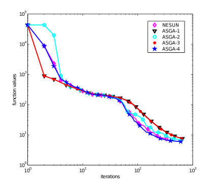
(a)

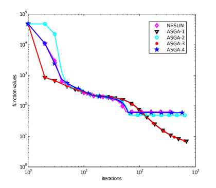
(b)

Figure 1: A comparison among NESUN, ASGA-1, ASGA-2, ASGA-3, and ASGA-4 for solving the $\ell_{1}$ minimization problem (91). For $\lambda=10^{-1}$, Subfigures (a) and (b) display the results for $\varepsilon=10^{-1}$ and $\varepsilon=10^{-4}$, respectively. The algorithms stopped after 30 seconds.

5.2 Elastic net minimization

Let us consider the underdetermined system (90), where the data is generated by (92). Since this problem is ill-conditioned, we apply a regularized least-squares with the elastic net regularizer, i.e.,

$$\min_{x\in\mathbb{R}^{n}}~{}~{}\displaystyle\frac{1}{2}\|y-Ax\|_{2}^{2}+\frac{1}{2}\lambda_{1}\|x\|_{2}^{2}+\lambda_{2}\|x\|_{1}$$ (93)

or

$$\begin{array}[]{ll}\min&~{}~{}\displaystyle\frac{1}{2}\|y-Ax\|_{2}^{2}+\frac{1}{2}\lambda_{1}\|x\|_{2}^{2}+\lambda_{2}\|x\|_{1}\\ \mathop{\rm s.t.~{}}&~{}~{}x\in\mathbf{x}=[\underline{x},\overline{x}],\end{array}$$ (94)

where $\lambda_{1},\lambda_{2}>0$ are regularization parameters. This problem is nonsmooth and strongly convex. By setting $f(x)=\frac{1}{2}\|y-Ax\|_{2}^{2}+\frac{1}{2}\lambda_{1}\|x\|_{2}^{2}$ and $\psi(x)=\lambda_{2}\|x\|_{1}$, we have that $f$ is $\lambda_{1}$-strongly convex and has Lipschitz continuous gradients with $\nu=1$ and $L_{\nu}=\|A\|_{2}^{2}+\lambda_{1}$.

We now run NSDSG, PGA, FISTA, NESCO, NESUN, ASGA-1, ASGA-2, ASGA-3, and ASGA-4 for solving the elastic net minimization problem (93) and NSDSG, NESCO, NESUN, ASGA-1, ASGA-2, ASGA-3, and ASGA-4 for solving the box-constrained version (94). The auxiliary problems of NESCO, NESUN, ASGA-1, ASGA-2, ASGA-3, and ASGA-4 are solved using the statements of Proposition 27. For (94), we set $\mathtt{\mathbf{x}=[-ones(5000,1),ones(5000,1)]}$. We stop the algorithms after 20 seconds of the running time. The results are summarized in Table 3.

Table 3: Numerical results of NSDSG, PGA, FISTA, NESCO, NESUN, ASGA-1, ASGA-2, ASGA-3, and ASGA-4 for the elastic net minimization problems (93) and (94). The first 10 problems stands for (93) and the remainder for (94). The algorithms were stopped after 20 seconds of the running time. $P$, $f_{b}$, and $N_{f}$ denote the problem number, the best function value, and the number of the function evaluations achieved by the algorithms, respectively.

$P$	$\lambda_{1}$	$\lambda_{2}$	NSDSG		PGA		FISTA		NESCO		NESUN		ASGA-1		ASGA-2		ASGA-3		ASGA-4
			$f_{b}$	$N_{f}$	$f_{b}$	$N_{f}$	$f_{b}$	$N_{f}$	$f_{b}$	$N_{f}$	$f_{b}$	$N_{f}$	$f_{b}$	$N_{f}$	$f_{b}$	$N_{f}$	$f_{b}$	$N_{f}$	$f_{b}$	$N_{f}$
1	$10^{-3}$	$1$	364.24	854	55.79	691	53.91	434	58.17	497	335.58	455	57.81	428	71.08	424	57.33	434	59.81	420
2	$10^{-3}$	$10^{-1}$	192.85	719	114.39	673	6.46	452	18.38	555	14.34	480	9.54	464	8.29	459	9.13	488	7.14	455
3	$10^{-3}$	$10^{-2}$	26.98	637	21.47	655	2.31	472	18.60	515	4.39	444	4.03	440	1.13	484	3.47	478	1.43	436
4	$10^{-3}$	$10^{-3}$	6.40	696	3.40	6.38	1.99	430	2.81	611	2.50	415	2.14	391	1.87	416	1.99	440	1.82	427
5	$10^{-3}$	$10^{-4}$	3.96	653	1.34	671	0.66	541	0.98	615	0.81	450	0.73	428	0.69	464	0.72	443	0.70	435
6	$10^{-4}$	$1$	499.59	664	61.73	710	59.29	430	65.17	559	408.85	431	62.96	459	79.11	422	62.65	467	65.22	521
7	$10^{-4}$	$10^{-1}$	194.57	654	114.54	677	6.35	511	19.82	555	10.21	448	10.00	442	9.14	433	9.35	465	6.83	446
8	$10^{-4}$	$10^{-2}$	24.49	757	20.56	674	1.67	593	16.81	603	4.10	456	4.27	431	1.31	440	3.57	476	1.25	463
9	$10^{-4}$	$10^{-3}$	5.26	660	4.76	657	1.73	446	2.33	5.85	2.04	425	1.74	448	1.63	433	1.64	500	1.59	442
10	$10^{-4}$	$10^{-4}$	4.86	6.49	1.16	605	0.28	420	0.67	511	0.31	415	0.28	412	0.28	408	0.28	405	0.28	410
11	$10^{-3}$	$1$	343.03	909	—	—	—	—	56.05	643	104.16	528	54.51	509	65.60	557	53.98	536	52.87	519
12	$10^{-3}$	$10^{-1}$	190.73	899	—	—	—	—	10.94	679	9.44	572	8.90	525	8.17	516	8.56	534	7.03	472
13	$10^{-3}$	$10^{-2}$	35.49	829	—	—	—	—	15.70	691	3.38	497	3.27	499	1.07	513	2.82	540	1.09	542
14	$10^{-3}$	$10^{-3}$	17.63	649	—	—	—	—	3.08	583	2.47	509	2.01	467	1.29	540	1.88	506	1.42	547
15	$10^{-3}$	$10^{-4}$	10.11	903	—	—	—	—	0.97	689	0.81	541	0.73	472	0.64	561	0.72	475	0.64	542
16	$10^{-4}$	$1$	353.73	900	—	—	—	—	64.31	629	336.19	510	61.04	556	70.63	532	61.26	509	59.89	522
17	$10^{-4}$	$10^{-1}$	176.44	892	—	—	—	—	15.59	567	7.67	498	7.79	539	6.99	540	8.37	477	6.20	439
18	$10^{-4}$	$10^{-2}$	23.37	821	—	—	—	—	15.58	695	2.42	566	3.46	491	1.06	521	3.02	529	1.25	463
19	$10^{-4}$	$10^{-3}$	8.20	906	—	—	—	—	2.32	603	1.92	525	1.66	481	1.18	548	1.57	530	1.42	492
20	$10^{-4}$	$10^{-4}$	12.70	858	—	—	—	—	0.49	663	0.29	549	0.28	504	0.27	564	0.28	517	0.27	539

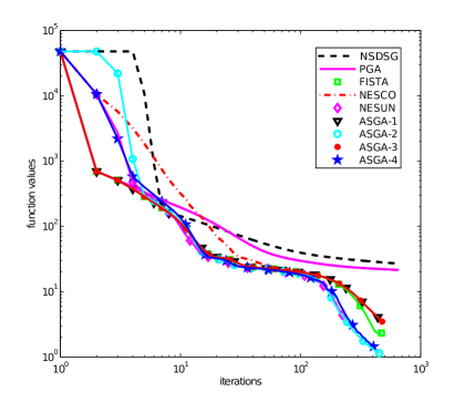
(a)

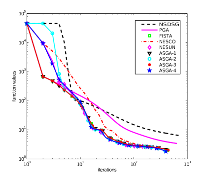
(b)

Figure 2: A comparison among NSDSG, PGA, FISTA, NESCO, NESUN, ASGA-1, ASGA-2, ASGA-3, and ASGA-4 for solving elastic net minimization problems (93): Subfigures (a) and (b) display comparisons of function values versus iterations for $\lambda_{1}=10^{-3},\lambda_{2}=10^{-2}$ and $\lambda_{1}=10^{-3},\lambda_{2}=10^{-3}$, respectively. The algorithms stopped after 20 seconds.

The results of Table 3 shows that the optimal methods FISTA, NESCO, NESUN, ASGA-1, ASGA-2, ASGA-3, and ASGA-4 outperforms NSDSG and PGA significantly as confirmed by their complexity analyses. It can also be seen that in many cases ASGA-2 and ASGA-4 performs better than NSDSG, PGA, FISTA, NESCO, NESUN, ASGA-1, and ASGA-2; however, in several cases they are comparable with FISTA, where FISTA is not generally applicable for constrained version (94). In addition, it is observable that ASGA-1 and ASGA-3 stay reasonable for a wide range of regularization parameters in contrast to ASGA-2 and ASGA-4. We therefore draw your attention to the Subfigures (a) and (b) of Figure 2 which give the function values versus iterations for (93) with two levels of regularization parameters $\lambda_{1}=10^{-3},\lambda_{2}=10^{-2}$ and $\lambda_{1}=10^{-3},\lambda_{2}=10^{-3}$.

5.3 Support vector machine

Let us consider learning with support vector machines (SVM) leading to a convex optimization problem with large data sets. In particular, we consider a binary classification, where the set of training data $(x_{1},y_{1}),\dots,(x_{m},y_{m})$ with $x_{i}\in\mathbb{R}^{n}$ and $y_{i}\in\{-1,1\}$, for $i=1,\dots,m$, are given. The aim is to find a classification rule from the training data, so that when given a new input $x$, we can assign a class $y\in\{-1,1\}$ to it. As SVM uses a classification rule that decides the class of $x$ based on the sign of $\langle x,w\rangle+w_{0}$, we need to choose the vector $w$ and the scalar $w_{0}$. These may be determined by solving the penalized problem

$$\begin{array}[]{ll}\min&~{}~{}\displaystyle\sum_{i=1}^{m}\left[1-y_{i}(\langle x_{i},w\rangle+w_{0})\right]_{+}+\lambda\phi(w)\\ \mathrm{s.t.}&~{}~{}w\in\mathbb{R}^{n},~{}w_{0}\in\mathbb{R},\end{array}$$ (95)

where $[z]_{+}=\max\{z,0\}$, and $\phi$ can be $\|\cdot\|_{1}$ (SVML1R), $\|\cdot\|_{2}^{2}$ (SVML22R), and $\frac{1}{2}\|\cdot\|_{2}^{2}+\|\cdot\|_{1}$ (SVML22L1R) (see, e.g., ShaS; ZhuRHT and references therein). For $\langle x,w\rangle=w^{T}x$, let us define

$$X:=\left(\begin{array}[]{c}y_{1}x_{1}^{T}\\ \vdots\\ y_{m}x_{m}^{T}\end{array}\right)\in\mathbb{R}^{m\times n},~{}~{}~{}A:=(X,y)\in\mathbb{R}^{m\times(n+1)},~{}~{}~{}\widetilde{w}:=\left(\begin{array}[]{l}w\\ w_{0}\end{array}\right)\in\mathbb{R}^{n+1}.$$

The problem (95) can be rewritten in the form

$$\begin{array}[]{ll}\min&~{}~{}\displaystyle\langle\mathbf{1},\left[\mathbf{1}-A\widetilde{w}\right]_{+}\rangle+\lambda\phi(w)\\ \mathrm{s.t.}&~{}~{}\widetilde{w}\in\mathbb{R}^{n+1},\end{array}$$ (96)

where $\left[\mathbf{1}-A\widetilde{w}\right]_{+}=\sup\{\mathbf{1}-A\widetilde{w},0\}$ and $\mathbf{1}\in\mathbb{R}^{m}$ is the vector of all ones. Typically $A$ is a dense matrix constructed by data points $x_{i}$ and $y_{i}$ for $i=1,\dots,m$. By setting $f(\widetilde{w})=\langle\mathbf{1},\left[\mathbf{1}-A\widetilde{w}\right]_{+}\rangle$ and $\psi(x)=\lambda\phi(w)$, it is clear that (96) is of the form (2), where $f$ is nonsmooth and its corresponding subgradient at $\widetilde{w}$ is given by

$$\nabla f(\widetilde{w})=-A^{T}\delta,$$

with

$$\forall i=1,\dots,m,~{}~{}~{}\delta_{i}:=\left\{\begin{array}[]{ll}1&~{}~{}\mathrm{if}~{}A_{i:}\widetilde{w}<1,\\ 0&~{}~{}\mathrm{if}~{}A_{i:}\widetilde{w}\geq 1,\end{array}\right.$$

For all $w_{1},w_{2}\in\mathbb{R}^{n}$, we have

$$\|\nabla f(w_{1})-\nabla f(w_{2})\|_{2}=\|A^{T}(\delta_{1}-\delta_{2})\|_{2}\leq\|A^{T}\|_{2}\|\delta_{1}-\delta_{2}\|_{2}\leq\sqrt{m}\|A^{T}\|_{2}:=L_{0},$$

where $A_{i:}$ denotes the $i$th row of $A$, for $i=1,\dots,m$. Therefore, $f$ satisfies (1) with $\nu=0$ and $L_{\nu}=L_{0}$.

Let us consider the problems SVML1R, SVML22R, and SVML22L1R for the leukemia data given by Golub et al. in Golub, available at the website Golub1. This dataset comes from a study of gene expression in two types of acute leukemias (acute myeloid leukemia (AML) and acute lymphoblastic leukemia (ALL)) and it consists of 38 training data points and 34 test data points. We apply SVML1R, SVML22R, and SVML22L1R to the training data points ($q=38$ and $n=7129$) with six levels of regularization parameters for each of SVML1R, SVML22R, and SVML22L1R. Since for SVML1R and SVML22L1R both $f$ and $\psi$ are nonsmooth functions, the algorithms PGA, FISTA, and NESCO cannot be applied to theses problems. Therefore, we only consider NSDSG, NESUN, ASGA-1, ASGA-2, ASGA-3, and ASGA-4 for solving these 3 problems with six levels of regularization parameters. In our implementation, the algorithms are stopped after 3 seconds of the running time. The associated results are given in Table 4 and Figure 3.

In spite of the fact that all the considered algorithms attain the complexity $\mathcal{O}(\varepsilon^{-2})$ for the problem (96), the results of Table 4 show that NESUN, ASGA-1, ASGA-2, ASGA-3, and ASGA-4 outperform NSDSG significantly, for all three problems (SVML1R, SVML22R, and SVML22L1R). For cases $\lambda\in\{10,1\}$, NESUN and ASGA-4 attain the better results than the others. For $\lambda\in\{10^{-1},10^{-2},10^{-3},10^{-4}\}$ and for all three problems, NESUN, ASGA-2, and ASGA-4 perform comparable but better than ASGA-1 and ASGA-3. However, ASGA-2 outperforms NESUN and ASGA-4 in the later case. We display the function values versus iterations of the considered algorithms in Subfigures (a) and (b) of Figure 3 for SVML22L1R with $\lambda=1$ and $\lambda=10^{-1}$, respectively. In Subfigure (a), NESUN and ASGA-4 outperform the others, while in Subfigure (b) ASGA-2 possesses the best result.

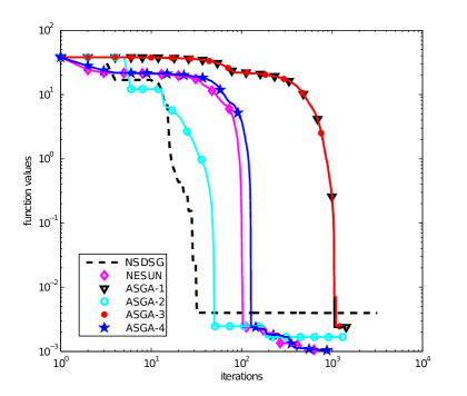
(a)

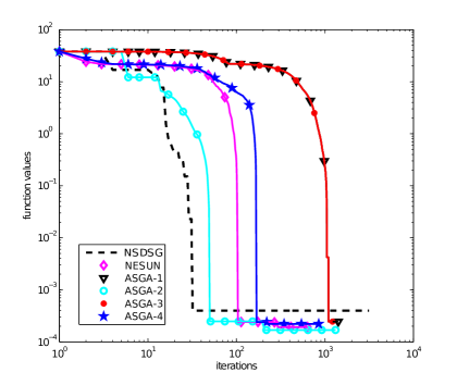
(b)

Figure 3: A comparison among NSDSG, NESUN, ASGA-1, ASGA-2, ASGA-3, and ASGA-4 for a binary classification with linear support vector machines (SVML22L1R) with $\lambda=1$ and $\lambda=10^{-1}$. The algorithms were stopped after 3 seconds.

Table 4: Numerical results of NSDSG, NESUN, ASGA-1, ASGA-2, ASGA-3, and ASGA-4 for the binary classification with linear support vector machines (96). The algorithms were stopped after 3 seconds of the running time. $f_{b}$ and $N_{f}$ denote the best function value and the number of function evaluations.

Prob. name	Reg. par.	NSDSG		NESUN		ASGA-1		ASGA-2		ASGA-3		ASGA-4
		$f_{b}$	$N_{f}$	$f_{b}$	$N_{f}$	$f_{b}$	$N_{f}$	$f_{b}$	$N_{f}$	$f_{b}$	$N_{f}$	$f_{b}$	$N_{f}$
SVML1R	$\lambda=10$	3.63 $\times 10^{-2}$	3641	9.97$\times 10^{-3}$	1482	2.43$\times 10^{-2}$	1682	1.51$\times 10^{-2}$	1524	2.37$\times 10^{-2}$	1247	1.21$\times 10^{-2}$	1239
SVML1R	$\lambda=1$	3.95$\times 10^{-3}$	3389	1.07$\times 10^{-3}$	1347	2.38$\times 10^{-3}$	1547	1.68$\times 10^{-3}$	1483	2.45$\times 10^{-3}$	1177	1.13$\times 10^{-3}$	1179
SVML1R	$\lambda=10^{-1}$	3.99$\times 10^{-4}$	3401	1.92$\times 10^{-4}$	1472	2.45$\times 10^{-4}$	1498	1.68$\times 10^{-4}$	1439	2.45$\times 10^{-4}$	1223	2.21$\times 10^{-4}$	1302
SVML1R	$\lambda=10^{-2}$	3.99$\times 10^{-5}$	3408	1.66$\times 10^{-5}$	1357	2.38$\times 10^{-5}$	1543	1.68$\times 10^{-5}$	1385	2.38$\times 10^{-5}$	1295	1.81$\times 10^{-5}$	1264
SVML1R	$\lambda=10^{-3}$	3.99$\times 10^{-6}$	3326	1.94$\times 10^{-6}$	1353	2.45$\times 10^{-6}$	1530	1.67$\times 10^{-6}$	1404	2.45$\times 10^{-6}$	1304	1.77$\times 10^{-6}$	1254
SVML1R	$\lambda=10^{-4}$	3.99$\times 10^{-7}$	3362	1.84$\times 10^{-7}$	1396	2.45$\times 10^{-7}$	1542	1.66$\times 10^{-7}$	1475	2.45$\times 10^{-7}$	1263	1.81$\times 10^{-7}$	1269
SVML22R	$\lambda=10$	7.96$\times 10^{-8}$	3442	2.75$\times 10^{-8}$	1454	2.91$\times 10^{-8}$	1598	3.01$\times 10^{-8}$	1490	2.91$\times 10^{-8}$	1236	2.76$\times 10^{-8}$	1276
SVML22R	$\lambda=1$	7.96$\times 10^{-9}$	3445	2.75$\times 10^{-9}$	1454	2.91$\times 10^{-9}$	1609	3.01$\times 10^{-9}$	1506	2.91$\times 10^{-9}$	1384	2.76$\times 10^{-9}$	1398
SVML22R	$\lambda=10^{-1}$	7.96$\times 10^{-10}$	3438	2.75$\times 10^{-10}$	1417	2.91$\times 10^{-10}$	1565	3.01$\times 10^{-10}$	1479	2.91$\times 10^{-10}$	1373	2.76$\times 10^{-10}$	1386
SVML22R	$\lambda=10^{-2}$	7.96$\times 10^{-11}$	3407	2.75$\times 10^{-11}$	1434	2.91$\times 10^{-11}$	1512	3.01$\times 10^{-11}$	1452	2.91$\times 10^{-11}$	1307	2.76$\times 10^{-11}$	1315
SVML22R	$\lambda=10^{-12}$	7.96$\times 10^{-12}$	3498	2.75$\times 10^{-12}$	1443	2.91$\times 10^{-12}$	1590	3.01$\times 10^{-12}$	1564	2.91$\times 10^{-12}$	1328	2.76$\times 10^{-12}$	1257
SVML22R	$\lambda=10^{-13}$	7.96$\times 10^{-13}$	3536	2.75$\times 10^{-13}$	1373	2.91$\times 10^{-13}$	1521	3.01$\times 10^{-13}$	1479	2.91$\times 10^{-13}$	1315	2.76$\times 10^{-13}$	1343
SVML22L1R	$\lambda=10$	3.65$\times 10^{-2}$	3179	1.01$\times 10^{-2}$	1247	2.43$\times 10^{-2}$	1393	1.51$\times 10^{-2}$	1192	2.37$\times 10^{-2}$	1156	1.23$\times 10^{-2}$	1166
SVML22L1R	$\lambda=1$	3.95$\times 10^{-3}$	3145	1.05$\times 10^{-3}$	1286	2.38$\times 10^{-3}$	1431	1.68$\times 10^{-3}$	1395	2.45$\times 10^{-3}$	1219	1.03$\times 10^{-3}$	1207
SVML22L1R	$\lambda=10^{-1}$	3.99$\times 10^{-4}$	3127	1.92$\times 10^{-4}$	1285	2.45$\times 10^{-4}$	1414	1.68$\times 10^{-4}$	1403	2.45$\times 10^{-4}$	1219	2.21$\times 10^{-4}$	1172
SVML22L1R	$\lambda=10^{-2}$	3.99$\times 10^{-5}$	3180	1.61$\times 10^{-5}$	1273	2.38$\times 10^{-5}$	1425	1.68$\times 10^{-5}$	1364	2.38$\times 10^{-5}$	1171	1.81$\times 10^{-5}$	1111
SVML22L1R	$\lambda=10^{-3}$	3.99$\times 10^{-6}$	3156	1.94$\times 10^{-6}$	1325	2.45$\times 10^{-6}$	1472	1.67$\times 10^{-6}$	1382	2.45$\times 10^{-6}$	1144	1.77$\times 10^{-6}$	1248
SVML22L1R	$\lambda=10^{-4}$	3.99$\times 10^{-7}$	3180	1.84$\times 10^{-7}$	1287	2.45$\times 10^{-7}$	1420	1.66$\times 10^{-7}$	1295	2.45$\times 10^{-7}$	1174	1.82$\times 10^{-7}$	1197

6 Final remarks

In this paper, we propose several novel (sub)gradient methods for solving large-scale convex composite minimization. More precisely, we give two estimation sequences approximating the objective function with some local and global information of the objective. For each of the estimation sequences, we give two iterative schemes attaining the optimal complexities for smooth, nonsmooth, weakly smooth, and smooth strongly convex problems. These schemes are optimal up to a logarithmic factors for nonsmooth strongly convex problems, and for weakly smooth strongly convex problems they attain a much better complexity than the complexity for weakly smooth convex problems. For each estimation sequence, the first scheme needs to know about the level of smoothness and the Hölder constant, while the second one is parameter-free (except for the strong convexity parameter which we set zero if it is not available) at the price of applying a backtracking line search. We then consider solutions of the auxiliary problems appearing in these four schemes and study the important cases appearing in applications that can be solved efficiently either in a closed form or by a simple iterative scheme. Considering some applicationsin the fields of sparse optimization and machine learning, we report numerical results showing the encouraging behavior of the proposed schemes.

Acknowledgement. I would like to thank Arnold Neumaier for his useful comments on this paper.