Monte Carlo with Determinantal Point Processes

Abstract

We show that repulsive random variables can yield Monte Carlo methods with faster convergence rates than the typical $N^{-1/2}$, where $N$ is the number of integrand evaluations. More precisely, we propose stochastic numerical quadratures involving determinantal point processes associated with multivariate orthogonal polynomials, and we obtain root mean square errors that decrease as $N^{-(1+1/d)/2}$, where $d$ is the dimension of the ambient space. First, we prove a central limit theorem (CLT) for the linear statistics of a class of determinantal point processes, when the reference measure is a product measure supported on a hypercube, which satisfies the Nevai-class regularity condition; a result which may be of independent interest. Next, we introduce a Monte Carlo method based on these determinantal point processes, and prove a CLT with explicit limiting variance for the quadrature error, when the reference measure satisfies a stronger regularity condition. As a corollary, by taking a specific reference measure and using a construction similar to importance sampling, we obtain a general Monte Carlo method, which applies to any measure with continuously derivable density. Loosely speaking, our method can be interpreted as a stochastic counterpart to Gaussian quadrature, which, at the price of some convergence rate, is easily generalizable to any dimension and has a more explicit error term.

1 Introduction

Numerical integration, or quadrature, refers to algorithms that approximate integrals

$$\int f(x)\mu({\rm d}x),$$ (1.1)

where $\mu$ is a finite positive Borel reference measure, and where $f$ ranges over some class of test functions $\mathscr{C}$. We assume for convenience that the support ${\rm Supp}(\mu)$ of $\mu$ is included in the $d$-dimensional hypercube $I^{d}=[-1,1]^{d}$, since one can recover this setting in most applications by means of appropriate transformations. For any given $N$, a quadrature algorithm outputs $N$ nodes $\mathbf{x}_{1},\ldots,\mathbf{x}_{N}\in I^{d}$ and weights $w_{1},\ldots,w_{N}\in\mathbb{R}$ so that the approximation

$$\sum_{i=1}^{N}w_{i}f(\mathbf{x}_{i})\approx\int f(x)\mu({\rm d}x)$$ (1.2)

is reasonable for every $f\in\mathscr{C}$. The nodes and weights depend on $N$, $\mu$, and can be realizations of random variables, but they are not allowed to depend on $f$. The quality of a quadrature algorithm is assessed through the approximation error

$$\mathscr{E}_{N}(f)=\sum_{i=1}^{N}w_{i}f(\mathbf{x}_{i})-\int f(x)\mu({\rm d}x)$$ (1.3)

and specifically its behaviour as $N\to\infty$.

Many quadrature algorithms have been developed: variations on Riemann summation (Davis and Rabinowitz, 1984), Gaussian quadrature (Gautschi, 2004), Monte Carlo methods (Robert and Casella, 2004), etc. In the remaining of Section 1, we quickly review three families of such methods to provide context for our contribution, which we then introduce in Section 1.5.

1.1 Gaussian quadrature

Let us first assume $d=1$, so that $\mu$ is supported on $I=[-1,1]$. Let $(\varphi_{k})_{k\in\mathbb{N}}$ be the orthonormal polynomials associated with this measure, that is, the family of polynomials such that $\varphi_{k}$ has degree $k$, positive leading coefficient, and $\int\varphi_{k}(x)\varphi_{\ell}(x)\mu({\rm d}x)=\delta_{k\ell}$ for every $k,\ell\in\mathbb{N}$. Gaussian quadrature, see e.g. (Davis and Rabinowitz, 1984; Gautschi, 2004; Brass and Petras, 2011) for general references, then corresponds to taking for nodes $\mathbf{x}_{1},\ldots,\mathbf{x}_{N}$ the zeros of the $N$th degree orthonormal polynomial $\varphi_{N}(x)$, which are real and simple. As for the weights, Gaussian quadrature corresponds to

$$w_{i}=\frac{1}{K_{N}(\mathbf{x}_{i},\mathbf{x}_{i})}\,,$$ (1.4)

where we introduced the $N$th Christoffel-Darboux kernel associated with $\mu$,

$$K_{N}(x,y)=\sum_{k=0}^{N-1}\varphi_{k}(x)\varphi_{k}(y).$$ (1.5)

This celebrated method is characterized by the property to be exact, i.e. $\mathscr{E}_{N}(f)=0$, for every polynomial function $f$ of degree up to $2N-1$. This is the highest possible degree such that this holds. Gaussian quadrature is thus particularly suitable when the test functions $f$ look like polynomials. For instance, $\mathscr{E}_{N}(f)$ decays exponentially fast when $f$ is analytic (Gautschi and Varga, 1983). However, although Gaussian quadrature is now two centuries old (Gauss, 1815), optimal rates of decay for the error $\mathscr{E}_{N}(f)$ do not seem to be known for less regular test functions, say $f\in\mathscr{C}^{1}$, in general. By using Jackson’s approximation theorem for algebraic polynomials, one can see that $\mathscr{E}_{N}(f)=\mathcal{O}(1/N)$ when $f\in\mathscr{C}^{1}$. Optimal decays have been recently investigated in the particular case of the Gauss-Legendre quadrature (Xiang and Bornemann, 2012; Xiang, 2016). However, even in the familiar Gauss-Jacobi quadrature, optimal rates are only conjectured.

Efficient computation of the nodes and weights in Gaussian quadrature has been an active topic of research. Classical approaches are based on the QR algorithm, such as the Golub-Welsch algorithm, see e.g. (Gautschi, 2004, Section 3.5) for a discussion. The computational cost of these QR approaches usually scales as $\mathcal{O}(N^{2})$. More recently, $\mathcal{O}(N)$ approaches have been proposed for specific choices of the reference measure (Glaser et al., 2007; Hale and Townsend, 2013), with parallelizable methods (Bogaert, 2014) further taking down costs.

Let us stress that Gaussian quadrature is intrinsically a one-dimensional method. Indeed, in the higher-dimensional setting where ${\rm Supp}(\mu)\subset I^{d}$, although one may define multivariate orthonormal polynomials associated with $\mu$, it is not possible to take for nodes the zeros of a multivariate polynomial. However, if $\mu$ is a product measure $\mu=\mu_{1}\otimes\cdots\otimes\mu_{d}$ with each $\mu_{j}$ supported on $I$, one could build a grid of nodes using $d$ one-dimensional Gaussian quadratures. But this has for consequence to rise up the one-dimensional error estimate for $\mathcal{E}_{N}(f)$ to a power $1/d$, which essentially makes Gaussian quadrature ineffective in higher dimensions than one or two. In fact, the same phenomenon arises for any other grid-like product of one-dimensional quadratures; this is commonly referred to as the curse of dimensionality.

1.2 Monte Carlo methods

Monte Carlo methods (Robert and Casella, 2004) correspond to picking up the $N$ nodes $({\mathbf{x}}_{i})$ in (1.2) as the realizations of random variables in $I^{d}$. For instance, assuming $\mu$ in (1.2) has a density $\omega$ with respect to the Lebesgue measure, importance sampling refers to taking the $({\mathbf{x}}_{i})$ to be i.i.d. realizations with a so-called proposal density $q$, and the weights to be

$$w_{i}=\frac{1}{N}\frac{\omega({\mathbf{x}}_{i})}{q({\mathbf{x}}_{i})}.$$ (1.6)

That way, $\mathscr{E}_{N}(f)$ has mean zero. Provided that

$$\mathbb{V}{\mathrm{ar}}\left[\frac{f(X)\omega(X)}{q(X)}\right]<\infty$$ (1.7)

where $X$ has density $q$, $\mathscr{E}_{N}(f)$ has a standard deviation decreasing as $N^{-1/2}$, and satisfies the classical central limit theorem:

$$\sqrt{N}\mathscr{E}_{N}(f)\xrightarrow[N\to\infty]{law}\mathcal{N}(0,\sigma_{f}^{2}),$$

where $\sigma_{f}^{2}$ equals (1.7). Let us stress that the cost of importance sampling is $\mathcal{O}(N)$, and that it can be easily parallelized.

When the ambient dimension $d$ becomes large, practitioners typically prefer Markov chain Monte Carlo (MCMC) methods over importance sampling. This means taking $w_{i}=1/N$ and nodes $({\mathbf{x}}_{i})$ to be the realization of a Markov chain with stationary distribution $\mu$, such as the Metropolis-Hastings chain. Under relatively weak conditions on the Markov chain and the integrand, $\sqrt{N}\mathscr{E}_{N}(f)$ then converges in distribution to a centered Gaussian variable; see e.g. (Douc et al., 2014, Theorem 7.32). The limiting variance usually grows more slowly with the dimension $d$ than for importance sampling; see (Belloni and Chernozhukov, 2009) for a proof in a simplified setting. This justifies the preferential use of MCMC for large $d$. In any case, the typical order of magnitude of the error $\mathscr{E}_{N}(f)$ for Monte Carlo methods is $N^{-1/2}$, which is often deemed a rather slow decay.

To retain the simplicity of implementation of Monte Carlo and achieve rates faster than $N^{-1/2}$, several authors have proposed postprocessing steps. For instance, Delyon and Portier (2016) proposed a variant of importance sampling that still takes nodes as independent draws from some proposal density $q$, but takes weights to be

$$w_{i}=\frac{1}{N}\frac{\omega({\mathbf{x}}_{i})}{\check{q}^{-i}({\mathbf{x}}_{i})},$$ (1.8)

where $\check{q}^{-i}$ is the so-called leave-one-out kernel estimator of the density $q$ of the nodes. Perhaps surprisingly, for smooth enough products $f\omega$ and the right tuning of kernel parameters, $\sqrt{N}\mathscr{E}_{N}(f)$ then converges in probability to zero. Exact rates are investigated by Delyon and Portier (2016), and a central limit theorem is proven. We further discuss their results in Section 4.

Another postprocessing technique with fast convergence relies on control variates (Glynn and Szechtman, 2002). Oates, Girolami, and Chopin (2017), for instance, sample nodes i.i.d. from $q$, and then split the nodes into two batches. The first batch is used to build an approximation $\hat{f}$ of the integrand $f$, with the constraint that $\int\hat{f}(x)\mu({\rm d}x)$ is known. The second batch is used to build an importance sampling estimator like (1.6) but targeting the residual $f-\hat{f}$. By carefully designing $\hat{f}$ and controlling the rate at which both batch sizes grow, (Oates et al., 2017, Theorem 2) obtain a mean square error in $N^{-7/6}$ under rather weak assumptions on measure $\mu$. The assumptions on the integrand $f$ are stronger, with $f$ to belong to a specific reproducing kernel Hilbert space. We note that Liu and Lee (2017) also propose a similar postprocessing approach, but the improvement on the rate is less explicit.

1.3 Quasi-Monte Carlo methods

Quasi-Monte Carlo methods (QMC; (Dick and Pilichshammer, 2010; Dick et al., 2013)) are deterministic constructions that focus on the uniform case, $\mu({\rm d}x)={\rm d}x$ in (1.2). The cornerstone of classical QMC is the Koksma-Hlawka inequality (Dick et al., 2013, Equation 3.15). This inequality bounds the error $\mathscr{E}_{N}(f)$ in (1.3) by the product of the star discrepancy of the nodes and the Hardy-Krause variation of $f$. The star discrepancy measures the departure of the empirical measure of the $N$ nodes from the uniform measure. Classical QMC methods aim at proposing efficient node constructions that minimize this star discrepancy. Some constructions guarantee a star discrepancy that asymptotically decreases as fast as $N^{-1}\log^{d-1}N$. This implies the same rate for $\mathscr{E}_{N}(f)$ provided $f$ has finite Hardy-Krause variation. While this seems faster than typical Monte Carlo methods in Section 1.2, the rate as a function of $N$ does not decrease until $N$ is exponential in $d$. Moreover, the Hardy-Krause variation is hard to manipulate in practice.

Modern QMC methods come up with more practical rates (Dick et al., 2013). For example, scrambled nets (Owen, 1997, 2008) are randomized QMC methods, meaning that a stochastic perturbation is applied to a deterministic QMC construction. The perturbation is built so that $\mathscr{E}_{N}(f)$ has mean $0$. Owen (1997) shows that only assuming $f$ is $L^{2}$, the standard deviation of $\mathscr{E}_{N}(f)$ is $o(N^{-1/2})$, that is, converges to zero faster than the traditional Monte Carlo rate. When $f$ is smooth enough, which requires at least that all mixed partial derivatives of $f$ of order less than $d$ are continuous, Owen (2008) further shows that the standard deviation is $\mathcal{O}(N^{-3/2-1/d}\log^{(d-1)/2}N)$. Again, this rate decreases only when $N$ is exponential in the dimension, but Owen (1997) shows that for finite $N$, randomized QMC cannot perform significantly worse than Monte Carlo.

Finally, we note that nonparametric control variates have also been studied for QMC and randomized QMC (Oates and Girolami, 2016). While bounds on the error still depend on the rather strong hypotheses of QMC, in particular the smoothness of the integrand, this postprocessing has the advantage of partially bypassing the need for the user to know the degree of smoothness in advance.

1.4 Bayesian quadrature

O’Hagan (1991) remarked that if we put a Gaussian process prior (Rasmussen and Williams, 2006) over the integrand, then the conditional of its integral given $N$ evaluations is a univariate Gaussian, with a closed-form mean and variance. Picking up nodes by sequentially minimizing this posterior variance yields a range of recent algorithms, such as kernel herding (Chen et al., 2010) or Bayesian quadrature (Huszár and Duvenaud, 2012). There is empirical evidence (Huszár and Duvenaud, 2012) that the error $\mathscr{E}_{N}(f)$ in Bayesian quadrature decreases faster than the Monte Carlo rate $N^{-1/2}$. There are theoretical results for hybrid methods between Monte Carlo and Bayesian quadrature (Briol et al., 2015), see Section 4 for further discussion.

The nodes and weights of Bayesian quadrature require inverting an $N\times N$ matrix and thus the computational cost of the method is $\mathcal{O}(N^{3})$. Although this cost may seem prohibitive, the approach is justified in some important applications where this cubic computational cost is negligible compared to the cost of one evaluation of the integrand.

1.5 Our contribution

Our main goal is to leverage repulsive particle systems to build a Monte Carlo method with standard deviation of the error decaying as $o(N^{-1/2})$. More precisely, the idea is to use correlated random variables for the quadrature nodes, interacting as strongly repulsive particles. Our motivation comes from specific models in random matrix theory (see Section 2.2 for references), for which the linear statistic $\sum f(x_{i})$ converges in distribution to a Gaussian, without requiring any normalizing factor. In this work, we focus on determinantal point processes (DPPs), which have received a lot of attention recently in probability and related fields, see for instance (Soshnikov, 2002; Lyons, 2003; Hough et al., 2006; Johansson, 2006; Kulesza and Taskar, 2012; Lavancier et al., 2015) for a general overview.

In any dimension $d$, we construct DPPs generating the nodes $\mathbf{x}_{1},\ldots,\mathbf{x}_{N}$ and appropriate weights $w_{i}$’s so that the error $\mathscr{E}_{N}(f)$ in (1.3) decreases rapidly, as $N\to\infty$. The general construction of our DPP for an arbitrary $\mu$ is relatively sophisticated, and will be the topic of Section 2.1. At this stage, we illustrate our results in the specific case where $\mu$ is the uniform measure on the hypercube $I^{d}$.

Theorem 1.

Let $(P_{k})_{k\in\mathbb{N}}$ be the Legendre polynomials defined by recurrence,

$$P_{0}(x):=1,\quad P_{1}(x):=x,\quad P_{k+1}(x):=\frac{2k+1}{k+1}xP_{k}(x)-\frac{k}{k+1}P_{k-1}(x),$$

and consider, for any $M\geqslant 1$ and $x,y\in\mathbb{R}^{d},$ the kernel

$$K_{N}(x,y):=\prod_{j=1}^{d}\sum_{k=0}^{M-1}\big{(}k+\frac{1}{2}\big{)}P_{k}(x_{j})P_{k}(y_{j}),$$

where $N:=M^{d}$. Let $\mathbf{x}_{1},\ldots,\mathbf{x}_{N}$ be sampled with density on $I^{d}$

$$\frac{1}{N!}\det\Big{[}K_{N}(x_{k},x_{\ell})\Big{]}_{k,\ell=1}^{N}.$$ (1.9)

Then, for any $\mathscr{C}^{1}$ function $f$ that is compactly supported within the open hypercube $(-1,1)^{d}$,

$$\mathbb{E}\left[\,\sum_{i=1}^{N}\frac{f(\mathbf{x}_{i})}{K_{N}(\mathbf{x}_{i},\mathbf{x}_{i})}\right]=\int_{I^{d}}f(x)\,{\rm d}x$$

and the quadratic error satisfies

$$\mathbb{E}\left[\,\sum_{i=1}^{N}\frac{f(\mathbf{x}_{i})}{K_{N}(\mathbf{x}_{i},\mathbf{x}_{i})}-\int_{I^{d}}f(x)\,{\rm d}x\right]^{2}=\mathcal{O}\left(\frac{1}{N^{1+1/d}}\right),$$

as $N\to\infty$. Moreover, we have a central limit theorem:

$$\sqrt{N^{1+1/d}}\left(\,\sum_{i=1}^{N}\frac{f(\mathbf{x}_{i})}{K_{N}(\mathbf{x}_{i},\mathbf{x}_{i})}-\int_{I^{d}}f(x)\,{\rm d}x\right)\xrightarrow[N\to\infty]{law}\mathcal{N}(0,\Omega_{f,1}^{2})\,,$$

where $\Omega_{f,1}$ has an explicit expression involving the regularity of $f$, see (2.17) below.

Sampling the distribution in (1.9), which is called a multivariate Legendre ensemble, can be done exactly in time $\mathcal{O}(N^{3})$, if we neglect the cost of rejection sampling steps, see Section 2.4. For the sake of illustration, a sample is shown in Figure 1(a) in the case $d=2$. For each $i$, the area of the disk centered at ${\mathbf{x}}_{i}$ is proportional to its weight $1/K_{N}({\mathbf{x}}_{i},{\mathbf{x}}_{i})$ in the quadrature rule of Theorem 1. Points are well-spread throughout the square, more so than under independent uniform sampling, with a visible accumulation along the border of the square compensated by smaller weights. The green lines on the side plots show the marginals of the uniform measure on the square. The histograms on the side plots are weighted empirical histograms of the sample.

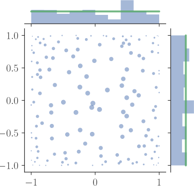
(a) 2D sample

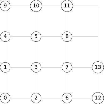
(b) The graded lexicographic order

Figure 1: 1(a) A weighted sample of size $N=150$ of the bivariate Legendre ensemble. 1(b) The graded lexicographic order in $d=2$: the lower left corner marks the origin $(0,0)\in\mathbb{N}^{2}$, and the circle with mark $k$ is at coordinates $\mathfrak{b}(k)$.

In this paper we prove a more general result than Theorem 1, where we consider a general class of measures instead of the uniform, and relax the assumption that the number of nodes $N$ is a $d$th power, see Theorem 3. For the latter, we need to introduce an ordering on multivariate monomials, see Section 2.2. We also provide an importance sampling (Theorem 4) and self-normalized importance sampling (Theorem 5) version of this result, having applications to Bayesian inference in mind.

Computationally, our method requires sampling from a DPP. The standard algorithm is $\mathcal{O}(N^{3})$ (Hough et al., 2006), plus some overhead due to using rejection sampling routines. As it stands, the applications of Monte Carlo with DPPs are thus naturally the same settings as Section 1.4, where the bottleneck is the evaluation of the integrand, not the generation of the nodes. Such settings arise in Bayesian inference for simulation-heavy sciences such as astrophysics (Trotta, 2006), ecology (Purves et al., 2013), or cell biology (Fink et al., 2011), where one evaluation of the integrand requires numerically solving large systems of differential equations. We comment in Section 2.4 on open avenues for faster sampling of specific DPPs, which would further widen the applicability of Monte Carlo with DPPs.

It turns out that, when $d=1$, our method is formally very similar to Gaussian quadrature, as described in Section 1.1. We basically replace the zeros of orthogonal polynomials by particles sampled from orthogonal polynomial ensembles (OP Ensembles), DPPs whose building blocks are orthogonal polynomials. Our contribution also has the advantage of generalizing more naturally to higher dimensions than Gaussian quadrature through multivariate OP Ensembles.

Monte Carlo with DPPs is to be classified somewhere between classical Monte Carlo methods and QMC methods, respectively described in Sections 1.2 and 1.3. It is very much similar to importance sampling, but with negatively correlated nodes. Simultaneously, it is more Monte Carlo than scrambled nets, as it does not randomize a posteriori a low discrepancy deterministic set of points, but rather incorporate the low discrepancy constraint into the randomization procedure. Our approach also bears similarity with postprocessing approaches to Monte Carlo with fast convergence of Section 1.2. Indeed, the fast convergence in our CLT is due to approximation results, much like nonparametric control variates. We further comment on this in Section 4.

The rest of the paper is organized as follows. In Section 2, we state our quadrature rules and theoretical results on the convergence of its error. In Section 3, we demonstrate our results in simple experimental settings. We conclude with some perspectives in Section 4. In Appendix A, we introduce key technical notions and give the outline of our proofs, the technical parts of the proofs being detailed in Appendices B and C. Appendix D contains additional experimental results.

2 Statement of the results

Notation.

All along this work, we write for convenience $I=[-1,1]$ and $I^{d}=[-1,1]^{d}$. Also, for any $0<\varepsilon<1$, we set $I_{\varepsilon}=[-1+\varepsilon,1-\varepsilon]$ and $I_{\varepsilon}^{d}=[-1+\varepsilon,1-\varepsilon]^{d}$. Finally, except when specified otherwise, a reference measure is a positive finite Borel measure with support ${\rm Supp}(\mu)\subset I^{d}$.

2.1 Determinantal point processes and multivariate OP Ensembles

2.1.1 Point processes and determinantal correlation functions

A simple point process (hereafter point process) on $I^{d}$ is a probability distribution $\mathbb{P}$ on finite subsets $\mathbf{S}$ of $I^{d}$. A classical exhaustive reference is (Daley and Vere-Jones, 2003), but we also refer the reader to (Hough et al., 2006), which is shorter and contains everything needed in this paper. Given a reference measure $\mu$, a point process has a $n$-correlation function $\rho_{n}$ if one has

$$\mathbb{E}\left[\sum_{\begin{subarray}{c}\mathbf{x}_{i_{1}},\ldots,\mathbf{x}_{i_{n}}\in\mathbf{S}\\ \mathbf{x}_{i_{1}}\neq\cdots\neq\mathbf{x}_{i_{n}}\end{subarray}}\varphi(\mathbf{x}_{i_{1}},\ldots,\mathbf{x}_{i_{n}})\right]=\int_{(I^{d})^{n}}\varphi(x_{1},\ldots,x_{n})\rho_{n}(x_{1},\ldots,x_{n})\mu^{\otimes n}({\rm d}x_{1},\ldots,{\rm d}x_{n})$$ (2.1)

for every bounded Borel function $\varphi:(I^{d})^{n}\to\mathbb{R}$, where the sum in (2.1) ranges over all pairwise distinct $n$-uplets of the random finite subset $\mathbf{S}$. The function $\rho_{n}$, provided it exists, thus encodes the correlations between distinct $n$-uplets of the random set $\mathbf{S}$. For instance, a Poisson process with intensity $\lambda:I^{d}\rightarrow\mathbb{R}_{+}$ is characterized by

$$\rho_{n}(x_{1},\dots,x_{n})=\prod_{i=1}^{n}\lambda(x_{i})$$ (2.2)

and ${\rm d}\mu(x)=\boldsymbol{1}_{I^{d}}(x){\rm d}x$. In that particular case, the correlation functions (2.2) are products of univariate terms, which can be paraphrased as there is no interaction between points in a Poisson point process. Finally, our definition (2.1) is easily seen to be equivalent to (Hough et al., 2006, Definition 1), where correlation functions are also called joint intensities. For ease of reference, we also note that correlation functions are called factorial moment densities in (Daley and Vere-Jones, 2003, Section 5.4).

A point process is determinantal (DPP) if there exists an appropriate kernel $K:I^{d}\times I^{d}\to\mathbb{R}$ or $\mathbb{C}$ such that the $n$-correlation function exists for every $n$ and reads

$$\rho_{n}(x_{1},\ldots,x_{n})=\det\Big{[}K(x_{k},x_{\ell})\Big{]}_{k,\ell=1}^{n},\qquad x_{1},\ldots,x_{n}\in I^{d}.$$ (2.3)

The kernel of a DPP thus encodes how the points in the random configurations interact. The existence of a point process with (2.3) as its correlation functions is, in general, a difficult question. It is easy to see that the kernel has to be positive definite, so that the right-hand side of (2.3) is always non-negative. But non-negativity is not sufficient for (2.3) to consistently define a point process.

A canonical way to construct DPPs is to define so-called projection DPPs, which generate configurations of $N$ points $\mathbb{P}$-almost surely, i.e. $\mathbf{S}=\{\mathbf{x}_{1},\ldots,\mathbf{x}_{N}\}$. More precisely, consider $N$ orthonormal functions $\varphi_{0},\ldots,\varphi_{N-1}$ in $L^{2}(\mu)$, that is, $\int\varphi_{k}(x)\varphi_{\ell}(x)\mu({\rm d}x)=\delta_{k\ell}$, and take for kernel

$$K_{N}(x,y)=\sum_{k=0}^{N-1}\varphi_{k}(x)\varphi_{k}(y).$$ (2.4)

In this setting, it turns out that the (permutation invariant) random variables $\mathbf{x}_{1},\ldots,\mathbf{x}_{N}$ with joint probability distribution

$$\frac{1}{N!}\det\Big{[}K_{N}(x_{i},x_{\ell})\Big{]}_{i,\ell=1}^{N}\prod_{i=1}^{N}\mu({\rm d}x_{i})$$ (2.5)

generate a DPP with kernel $K_{N}(x,y)$. (Hough et al., 2006, Section 2) gives a proof that (2.5) yields (2.3) with $K=K_{N}$.

For further information on determinantal point processes, we refer the reader to (Macchi, 1975; Hough et al., 2006; Johansson, 2006; Soshnikov, 2000; Lyons, 2003; Kulesza and Taskar, 2012; Lavancier et al., 2015).

2.1.2 Multivariate OP Ensembles

In the one-dimensional setting, we can for instance build a DPP using (2.5) with $\varphi_{0},\text{...},\varphi_{N-1}$ the $N$ lowest degree orthonormal polynomials associated with the reference measure $\mu$. Such DPPs are known as OP Ensembles and have been popularized by random matrix theory, see e.g. (König, 2005) for an overview.

Our contribution involves a higher-dimensional generalization of OP Ensembles, relying on multivariate orthonormal polynomials, which we now introduce. Given a reference measure $\mu$, assume it has well-defined multivariate orthonormal polynomials, meaning that $\int P^{2}(x)\mu({\rm d}x)>0$ for every non-trivial polynomial $P$. This is for instance true if $\mu(A)>0$ for some non-empty open set $A\subset I^{d}$. Now choose an ordering for the multi-indices $(\alpha_{1},\ldots,\alpha_{d})\in\mathbb{N}^{d}$, that is, pick a bijection $\mathfrak{b}:\mathbb{N}\to\mathbb{N}^{d}$. This gives an ordering of the monomial functions $(x_{1},\ldots,x_{d})\mapsto x_{1}^{\alpha_{1}}\cdots x_{d}^{\alpha_{d}}$, to which one applies the Gram-Schmidt algorithm. This yields a sequence of orthonormal polynomial functions $(\varphi_{k})_{k\in\mathbb{N}}$, the multivariate orthonormal polynomials. In this work, we use a specific bijection $\mathfrak{b}$ defined in Section 2.1.3.

Equipped with this sequence $(\varphi_{k})_{k\in\mathbb{N}}$ of multivariate orthonormal polynomials, we finally consider for every $N$ the DPP associated with the associated kernel (2.4), that we refer to as the multivariate OP Ensemble associated with a reference measure $\mu$. When $d=1$, it reduces to the classical OP Ensemble.

2.1.3 The graded lexicographic order and the bijection $\mathfrak{b}$

We consider the bijection $\mathfrak{b}$ associated with the graded (with respect to the sup norm) alphabetic order on $\mathbb{N}^{d}$. We start with the usual lexicographic order on $\mathbb{N}^{d}$, defined by saying that $(\alpha_{1},\ldots,\alpha_{d})<_{{\rm lex}}(\beta_{1},\ldots,\beta_{d})$ if there exists $j\in\{1,\ldots,d\}$ such that $\alpha_{i}=\beta_{i}$ for every $i<j$ and $\alpha_{j}<\beta_{j}$. Now we define the graded lexicographic order as follows. We say that $(\alpha_{1},\ldots,\alpha_{d})<(\beta_{1},\ldots,\beta_{d})$ if either $\max\{\alpha_{1},\ldots,\alpha_{d}\}<\max\{\beta_{1},\ldots,\beta_{d}\}$ or $\max\{\alpha_{1},\ldots,\alpha_{d}\}=\max\{\beta_{1},\ldots,\beta_{d}\}$ and $(\alpha_{1},\ldots,\alpha_{d})<_{{\rm lex}}(\beta_{1},\ldots,\beta_{d})$. Moreover, from now on we specify the bijection $\mathfrak{b}$ to be the unique bijection $\mathbb{N}\to\mathbb{N}^{d}$ increasing for this order. Otherly put, set $\mathfrak{b}(0)=(0,\ldots,0)$ and $\mathfrak{b}(n)=\min\;\mathbb{N}^{d}\setminus\big{\{}\mathfrak{b}(0),\ldots,\mathfrak{b}(n-1)\big{\}}$ by induction, where the minimum refers to the graded lexicographic order. An important feature of this ordering on which our proofs rely is that, for every $M\geqslant 1$, the set of the first $M^{d}$ indices $\{\mathfrak{b}(0),\ldots,\mathfrak{b}(M^{d}-1)\}$ matches the discrete hypercube

$$\mathcal{C}_{M}=\Big{\{}\boldsymbol{n}\in\mathbb{N}^{d}:\;0\leqslant n_{1},\ldots,n_{d}\leqslant M-1\Big{\}}.$$ (2.6)

The indices between $\mathfrak{b}(M^{d}-1)$ and $\mathfrak{b}(M^{d+1}-1)$ then fill the layer $\mathcal{C}_{M+1}\setminus\mathcal{C}_{M}$ by following the usual lexicographic order. For better intuition, we illustrate the order $\mathfrak{b}$ for $d=2$ in Figure 1(b); observe how each layer is filled one after the other.

We are now in position to state our first result on multivariate OP Ensembles, which is the cornerstone for the Monte Carlo methods we introduce later in Section 2.3.

2.2 A central limit theorem for multivariate OP Ensembles

Several central limit theorems (CLTs) have been obtained for determinantal point processes and related models in random matrix theory, but only when the random configurations lie in a one- or two-dimensional domain. See for instance (Johansson, 1997, 1998; Diaconis and Evans, 2001; Soshnikov, 2002; Pastur, 2006; Rider and Virág, 2007; Popescu, 2009; Kriecherbauer and Shcherbina, 2010; Ameur et al., 2011, 2015; Berman, 2012; Shcherbina, 2013; Breuer and Duits, 2017, 2016; Johansson and Lambert, 2018; Lambert, 2018, 2015) for a non-exhaustive list. Although DPPs on higher-dimensional supports have attracted attention in complex geometry (Berman, 2009a, b, 2018, 2014), in statistics (Lavancier et al., 2015; Møller et al., 2015), and in physics (Torquato et al., 2008; Scardicchio et al., 2009), it seems no CLT has been established yet when $d\geqslant 3$.

Our first result for multivariate OP Ensembles is a CLT for $\mathscr{C}^{1}$ test functions when the reference measure $\mu$ is a product of $d$ Nevai-class probability measures on $I$. The exact definition of the Nevai class is postponed until Definition 1, but we now give a simple sufficient condition. As a consequence of Denisov–Rakhmanov’s theorem (see Theorem 6), if a measure on $I$ has for Lebesgue decomposition $\mu({\rm d}x)=\omega(x){\rm d}x+\mu_{s}$ (where $\mu_{s}$ is orthogonal to the Lebesgue measure) with $\omega(x)>0$ almost everywhere, then $\mu$ is Nevai-class. Denote by $(T_{k})_{k\in\mathbb{N}}$ the normalized Chebyshev polynomials, defined on $I$ by

$$T_{0}=1,\qquad T_{k}(\cos\theta)=\sqrt{2}\cos(k\theta),\qquad k\geqslant 1.$$

Theorem 2.

Let $\mu$ be a reference measure with ${\rm Supp}(\mu)\subset I^{d}$, and assume $\mu=\mu_{1}\otimes\cdots\otimes\mu_{d}$ where each $\mu_{j}$ is Nevai class (see Definition 1). If $\mathbf{x}_{1},\ldots,\mathbf{x}_{N}$ stands for the associated multivariate OP Ensemble associated with $\mu$, then for every $f\in\mathscr{C}^{1}(I^{d},\mathbb{R})$, we have

$$\frac{1}{\sqrt{N^{1-1/d}}}\left(\ \sum_{i=1}^{N}f(\mathbf{x}_{i})-\mathbb{E}\left[\,\sum_{i=1}^{N}f(\mathbf{x}_{i})\right]\right)\xrightarrow[N\to\infty]{law}\mathcal{N}(0,\sigma_{f}^{2}),$$

where

$$\sigma_{f}^{2}=\frac{1}{2}\sum_{k_{1},\ldots,k_{d}=0}^{\infty}(k_{1}+\cdots+k_{d}){\hat{f}(k_{1},\ldots,k_{d})}^{2}$$ (2.7)

and

$$\hat{f}(k_{1},\ldots,k_{d})=\int_{I^{d}}f(x_{1},\ldots,x_{d})\prod_{j=1}^{d}T_{k_{j}}(x_{j})\frac{{\rm d}x_{j}}{\pi\sqrt{1-x_{j}^{2}}}.$$ (2.8)

When $d=1$, Theorem 2 was obtained by Breuer and Duits (2017), see also (Lambert, 2015) for an alternative proof, but the higher-dimensional case $d\geqslant 2$ is novel. We shall restrict to $d\geqslant 2$ for the proof of the theorem, which is deferred to Section B. Let us now make a few remarks concerning the statement of Theorem 2.

Remark 1.

The limiting variance $\sigma_{f}^{2}$ does not depend on the reference measure $\mu$.

Remark 2.

By making the change of variables $x_{j}=\cos\theta_{j}$, we obtain

$$\hat{f}(k_{1},\ldots,k_{d})=\frac{(\sqrt{2})^{|\{j:\;k_{j}\neq 0\}|}}{\pi^{d}}\int_{[0,\pi]^{d}}f(\cos\theta_{1},\ldots,\cos\theta_{d})\prod_{j=1}^{d}\cos(k_{j}\theta_{j}){\rm d}\theta_{j},$$

which is, up to a multiplicative factor, a usual Fourier coefficient.

As a side note, we obtain that the limiting variance in Theorem 2 is dominated by an explicit integral, that may be of interest to bound $\sigma_{f}^{2}$ in practice.

Proposition 1.

For any $f\in\mathscr{C}^{1}(I^{d},\mathbb{R})$, we have the inequality

$$\sigma_{f}^{2}\leqslant\frac{1}{2}\sum_{\alpha=1}^{d}\int_{I^{d}}\Big{(}\sqrt{1-x_{\alpha}^{2}}\,\partial_{\alpha}f(x_{1},\ldots,x_{d})\Big{)}^{2}\,\prod_{j=1}^{d}\frac{{\rm d}x_{j}}{\pi\sqrt{1-x_{j}^{2}}}.$$ (2.9)

It will appear from the proof we provide in Section A.3 that this inequality is sharp, since equality holds whenever $f$ is a linear combination of monomials $x_{1}^{\alpha_{1}}\cdots x_{d}^{\alpha_{d}}$ with $\alpha_{j}\in\{0,1\}$; see (A.26).

We now turn to Monte Carlo methods based on Theorem 2.

2.3 Monte Carlo methods based on determinantal point processes

Consider a reference measure $\mu$ with support inside $I^{d}$, having well-defined multivariate orthonormal polynomials (say, $\mu(A)>0$ for some open set $A\subset I^{d}$). Let $K_{N}(x,y)$ be the $N$th Christoffel-Darboux kernel for the associated multivariate OP Ensemble, namely

$$K_{N}(x,y)=\sum_{k=0}^{N-1}\varphi_{k}(x)\varphi_{k}(y),$$ (2.10)

where $(\varphi_{k})_{k\in\mathbb{N}}$ is the sequence of multivariate orthonormal polynomials associated with $\mu$ and the graded lexicographic order, see Section 2.1.3. Our quadrature rule is as follows: take for nodes $\mathbf{x}_{1},\ldots,\mathbf{x}_{N}$ the random points coming from the multivariate OP Ensemble, namely with joint density (2.5), and for weights $w_{i}=1/K_{N}(\mathbf{x}_{i},\mathbf{x}_{i})$. Thus, for any $\mu$-integrable function $f$, our estimator of $\int f(x)\mu({\rm d}x)$ reads

$$\sum_{i=1}^{N}\frac{f(\mathbf{x}_{i})}{K_{N}(\mathbf{x}_{i},\mathbf{x}_{i})}.$$ (2.11)

One can readily see by taking $n=1$ in (2.1)–(2.4) that the estimator (2.11) is unbiased,

$$\mathbb{E}\left[\ \sum_{i=1}^{N}\frac{f(\mathbf{x}_{i})}{K_{N}(\mathbf{x}_{i},\mathbf{x}_{i})}\ \right]=\int f(x)\mu({\rm d}x).$$ (2.12)

Remark 3.

For $d=1$, comparing (2.11) to (1.4)–(1.5) yields that our method matches Gaussian quadrature except for the nodes, since we replace the zeros of the univariate orthogonal polynomial $\varphi_{N}$ by random points drawn from an OP Ensemble. In fact, this replacement is not aberrant since zeros of orthogonal polynomials and particles of associated OP Ensembles get arbitrarily close with high probability as $N\to\infty$, see (Hardy, 2015) for further information and generalizations. Notice however that our quadrature rule has the advantage to make sense in any dimension $d$.

Our next result is a CLT for (2.11), thus giving a precise rate of decay for the error made in the approximation, provided we make regularity assumptions on $\mu$ and on the class $\mathscr{C}$ of test functions $f$. More precisely, recalling the notation $I_{\varepsilon}^{d}=[-1+\varepsilon,1-\varepsilon]^{d}$, we consider

$$\mathscr{C}=\Big{\{}f\in\mathscr{C}^{1}(I^{d},\mathbb{R}):\;{\rm Supp}(f)\subset I_{\varepsilon}^{d}\mbox{ for some }\varepsilon>0\Big{\}}.$$ (2.13)

As for the reference measure, we shall assume $\mu$ is a product measure with a density which is $\mathscr{C}^{1}$ and positive on the open set $(-1,1)^{d}$. Set for convenience

$$\omega_{eq}^{\otimes d}(x)=\prod_{j=1}^{d}\frac{1}{\pi\sqrt{1-x_{j}^{2}}} \ ,\qquad x\in I^{d}.$$ (2.14)

Theorem 3 (Crude Monte Carlo with OP Ensembles).

Let $\mu({\rm d}x)=\omega(x){\rm d}x$ be a product reference measure with $\omega(x)=\omega_{1}(x_{1})\cdots\omega_{d}(x_{d})$ and ${\rm Supp}(\mu)\subset I^{d}$. Assume $\omega$ is $\mathscr{C}^{1}$ and positive on the open set $(-1,1)^{d}$, and satisfies: for every $\varepsilon>0$,

$$\frac{1}{N}\sup_{x\in I_{\varepsilon}^{d}}\left|\nabla K_{N}(x,x)\right|<\infty.$$ (2.15)

If $\mathbf{x}_{1},\ldots,\mathbf{x}_{N}$ stands for the multivariate OP Ensemble associated with $\mu$, then for every $f\in\mathscr{C}$, we have for the mean square error of the estimator,

$$\lim_{N\to\infty}N^{1+1/d}\ \mathbb{E}\left[\left(\ \sum_{i=1}^{N}\frac{f(\mathbf{x}_{i})}{K_{N}(\mathbf{x}_{i},\mathbf{x}_{i})}-\int f(x)\mu({\rm d}x)\right)^{2}\ \right]=\Omega_{f,\omega}^{2}\ .$$ (2.16)

where, see (2.8),

$$\Omega_{f,\omega}^{2}=\frac{1}{2}\sum_{k_{1},\ldots,k_{d}=0}^{\infty}(k_{1}+\cdots+k_{d})\widehat{\left(\frac{f\omega}{\omega_{eq}^{\otimes d}}\right)}(k_{1},\ldots,k_{d})^{2}.$$ (2.17)

Moreover, we have the central limit theorem,

$$\sqrt{N^{1+1/d}}\left(\ \sum_{i=1}^{N}\frac{f(\mathbf{x}_{i})}{K_{N}(\mathbf{x}_{i},\mathbf{x}_{i})}-\int f(x)\mu({\rm d}x)\right)\xrightarrow[N\to\infty]{law}\mathcal{N}\big{(}0,\Omega_{f,\omega}^{2}\big{)},$$

We will discuss the assumptions of Theorem 3 in Section A.4 but let us already state that, as it will appear in the proof, (2.15) can be replaced by the weaker but technically involved Assumption 1. We restricted ourselves to (2.15) for the sake of presentation, as it already covers the Jacobi case. Indeed, we prove the following result in Section A.4.

Proposition 2.

Given any parameters $\alpha_{1},\beta_{1},\ldots,\alpha_{d},\beta_{d}>-1$, the reference measure

$$\mu({\rm d}x)=\prod_{j=1}^{d}(1-x_{j})^{\alpha_{j}}(1+x_{j})^{\beta_{j}}\boldsymbol{1}_{I}(x_{j}){\rm d}x_{j},$$ (2.18)

satisfies the assumptions of Theorem 3.

Hereafter, we call measures of the form (2.18) Jacobi measures. From a practical point of view, Theorem 3 requires knowledge on the measure $\mu$, in particular all its moments should be known, since we need the corresponding orthonormal polynomials. This is the case for most applications of Gaussian quadrature, where the reference measure is such that orthonormal polynomials are computable, like Jacobi measures (2.18) for instance. When the moments of $\mu$ are not known or when $\mu$ is not separable, we propose an importance sampling result in Theorem 4, which shifts most hypotheses onto an instrumental density $q$. Note however that Theorem 4 still requires that we can evaluate the density $\omega$ of $\mu$ pointwise.

Theorem 4 (Importance sampling with OP Ensembles).

Let $\mu({\rm d}x)=\omega(x){\rm d}x$ be a reference measure on $I^{d}$ with a $\mathscr{C}^{1}$ density $\omega$ on the open set $(-1,1)^{d}$. Consider a measure $q(x){\rm d}x$ satisfying the assumptions of Theorem 3, let $K_{N}(x,y)$ be the $N$th Christoffel-Darboux kernel associated with $q(x){\rm d}x$, and $\mathbf{x}_{1},\ldots,\mathbf{x}_{N}$ the associated multivariate OP Ensemble. Then, for every $f\in\mathscr{C}$, we have

$$\mathbb{E}\left[\ \sum_{i=1}^{N}\frac{f(\mathbf{x}_{i})}{K_{N}(\mathbf{x}_{i},\mathbf{x}_{i})}\frac{\omega(\mathbf{x}_{i})}{q(\mathbf{x}_{i})}\ \right]=\int f(x)\mu({\rm d}x),$$ (2.19)

and we have for the mean square error of the estimator,

$$\lim_{N\to\infty}N^{1+1/d}\ \mathbb{E}\left[\left(\ \sum_{i=1}^{N}\frac{f(\mathbf{x}_{i})}{K_{N}(\mathbf{x}_{i},\mathbf{x}_{i})}\frac{\omega(\mathbf{x}_{i})}{q(\mathbf{x}_{i})}-\int f(x)\mu({\rm d}x)\right)^{2}\ \right]=\Omega_{f,\omega}^{2}\ ,$$ (2.20)

where $\Omega_{f,\omega}^{2}$ is the same as (2.17). Moreover, we have the central limit theorem,

$$\sqrt{N^{1+1/d}}\left(\ \sum_{i=1}^{N}\frac{f(\mathbf{x}_{i})}{K_{N}(\mathbf{x}_{i},\mathbf{x}_{i})}\frac{\omega(\mathbf{x}_{i})}{q(\mathbf{x}_{i})}-\int f(x)\mu({\rm d}x)\right)\xrightarrow[N\to\infty]{law}\mathcal{N}\big{(}0,\Omega_{f,\omega}^{2}\big{)}.$$ (2.21)

Indeed, Theorem 4 follows from Theorem 3 by taking $f\omega/q$ for test function with $f\in\mathscr{C}$ and $q(x){\rm d}x$ for reference measure.

Remark 4.

From a classical importance sampling perspective, it is surprising that the limiting variance in (2.21) does not depend on the proposal density $q$.

In most applications to Bayesian inference, $\mu$ is a probability measure, but its density $\omega$ can only be evaluated up to a multiplicative constant. A classical trick is to rely on self-normalized importance sampling. Theorem 5 states a central limit theorem for such an estimator.

Theorem 5 (Self-normalized importance sampling with OP Ensembles).

Let $\mu({\rm d}x)=\omega(x){\rm d}x=\omega_{u}(x){\rm d}x/Z$ be a reference probability measure on $I^{d}$ with a $\mathscr{C}^{1}$ density $\omega$ on the open set $(-1,1)^{d}$. We further assume that $\mu$ is supported in $I_{\varepsilon}^{d}=[-1+\varepsilon,1-\varepsilon]^{d}$. As in Theorem 4, consider a measure $q(x){\rm d}x$ satisfying the assumptions of Theorem 3, let $K_{N}(x,y)$ be the $N$th Christoffel-Darboux kernel associated with $q(x){\rm d}x$, and $\mathbf{x}_{1},\ldots,\mathbf{x}_{N}$ the associated multivariate OP Ensemble. Finally, for convenience, we let

$$\mathscr{I}_{N}(g)=\sum_{i=1}^{N}\frac{g(\mathbf{x}_{i})}{K_{N}(\mathbf{x}_{i},\mathbf{x}_{i})}\frac{\omega_{u}(\mathbf{x}_{i})}{q(\mathbf{x}_{i})},\quad g:I^{d}\rightarrow\mathbb{R}.$$

Then, for every $f\in\mathscr{C}$, we have

$$\sqrt{N^{1+1/d}}\left(\mathscr{I}_{N}(f)/\mathscr{I}_{N}(1)-\int f(x)\mu({\rm d}x)\right)\xrightarrow[N\to\infty]{law}\mathcal{N}\big{(}0,\Xi_{f,\omega}^{2}\big{)},$$ (2.22)

where

$$\Xi_{f,\omega}^{2}=\Omega^{2}_{f,\omega}-2c_{f,\omega}\int f{\rm d}\mu+\Omega_{1,\omega}^{2}\left(\int f{\rm d}\mu\right)^{2}\geqslant 0,$$

and

$$c_{f,\omega}=\frac{1}{2}\sum_{k_{1},\ldots,k_{d}=0}^{\infty}(k_{1}+\cdots+k_{d})\widehat{\left(\frac{f\omega}{\omega_{eq}^{\otimes d}}\right)}(k_{1},\ldots,k_{d})\times\widehat{\left(\frac{\omega}{\omega_{eq}^{\otimes d}}\right)}(k_{1},\ldots,k_{d}).$$

We prove Theorem 5 in Section A.5 using the same arguments as for classical importance sampling (Schervish, 2012, Section 7.1.3), but replacing the standard CLT by Theorem 4.

2.4 Sampling a multivariate OP Ensemble

For Monte Carlo with DPPs to be a practical tool, we need to be able to sample realizations of the random variables $\mathbf{x}_{1},\ldots,\mathbf{x}_{N}$ with joint density (2.5). Hough et al. (2006) give an algorithm for sampling generic DPPs, which we use here; see also (Scardicchio et al., 2009; Lavancier et al., 2015; Olver et al., 2015) for more details. In terms of code, a companion Python package to the current paper is available, which implements the OPE sampling described in this section and used later for the experiments in Section 3. A more efficient implementation of the same OPE sampling algorithm, along with most known DPP sampling algorithms, can also be found in the Python package DPPy (Gautier, Bardenet, and Valko, 2018).

The algorithm is based on the fact that the chain rule for the joint distribution (2.5) is available as

$$\frac{1}{N!}\det\Big{[}K_{N}(x_{i},x_{\ell})\Big{]}_{i,\ell=1}^{N}\prod_{i=1}^{N}\mu({\rm d}x_{i})=\prod_{i=1}^{N}\frac{1}{N-i+1}\Big{\|}P_{H_{i-1}}K_{N}(x_{i},\cdot)\Big{\|}_{L^{2}(\mu)}^{2}\mu({\rm d}x_{i}).$$ (2.23)

In (2.23), $P_{H}$ is the orthogonal projection onto a subspace $H$ of $L^{2}(\mu)$,

$$H_{0}=\text{Span}(\varphi_{0},\dots,\varphi_{N-1}),$$

and $H_{i-1}$ is the orthocomplement in $H_{0}$ of

$$\text{Span}\left(K_{N}(x_{\ell},\cdot),\;1\leqslant\ell\leqslant i-1\right)$$

for every $i>1$. In particular, all the terms in the product of the RHS of (2.23) are probability measures (Hough et al., 2006, Proposition 19). Notice that the factorization (2.23) is the equivalent of the “base times height” formula that computes the squared volume of the parallelotope generated by the vectors $(\varphi_{0}(x_{i}),\ldots,\varphi_{N-1}(x_{i}))$ for $1\leqslant i\leqslant N$.

Using the normal equations, we can also rewrite each term in the product (2.23)

$$\Big{\|}P_{H_{i-1}}K_{N}(x_{i},\cdot)\Big{\|}_{L^{2}(\mu)}^{2}=\begin{cases}K_{N}(x_{1},x_{1})&\text{if }i=1,\\ K_{N}(x_{i},x_{i})-{\bf k}_{1:i-1}(x_{i})^{T}{\bf K}_{1:i-1}^{-1}{\bf k}_{1:i-1}(x_{i})&\text{else,}\end{cases}$$ (2.24)

where

$${\bf k}_{1:i-1}(\cdot)=\left(K_{N}(x_{1},\cdot),\dots,K_{N}(x_{i-1},\cdot)\right)^{T}$$

and

$${\bf K}_{1:i-1}=\Big{[}K_{N}(x_{k},x_{\ell})\Big{]}_{1\leqslant k,\ell\leqslant i-1}.$$

Remark 5.

Equation (2.24) will be familiar to users of Gaussian processes (GPs; Rasmussen and Williams 2006): the unnormalized conditional densities (2.24) are the incremental posterior variances in a GP model with the same kernel.

Remark 6.

Evaluating (2.24) requires evaluating $K_{N}$, or equivalently the polynomials $\varphi_{k}$ for $k=0,\dots,N-1$. This can be efficiently implemented using the three-term recurrence relations for orthogonal polynomials, when the recurrence coefficients are known; see e.g. (Gautschi, 2004, Section 1.3) for whom this recurrence is “arguably the single most important piece of information for the constructive and computational use of orthogonal polynomials”.

In a nutshell, sampling a multivariate OPE amounts to sampling from each conditional (2.24) in the chain rule (2.23), one after the other. The only thing left to specify is how we sample each conditional. In this paper, we propose to sample each conditional by rejection sampling (Robert and Casella, 2004, Section 2.3). This requires proposal densities $(q_{i})_{1\leqslant i\leqslant N}$ and tight bounds on the density ratios

$$\frac{\Big{\|}P_{H_{i-1}}K_{N}(x,\cdot)\Big{\|}_{L^{2}(\mu)}^{2}\omega(x)}{q_{i}(x)},\quad 1\leqslant i\leqslant N,$$ (2.25)

when $\mu({\rm d}x)=\omega(x){\rm d}x$. A theorem of Totik, which we recall later as Theorem 9, gives light conditions on $\omega$, under which

$$\frac{N}{K_{N}(x,x)}\rightarrow\frac{\omega(x)}{\omega_{\text{eq}}(x)},$$

uniformly on $I_{\varepsilon}^{d}$. This suggests choosing

$$q_{i}(x)=q(x)=\omega_{eq}^{\otimes d}(x)=\prod_{j=1}^{d}\frac{1}{\pi\sqrt{1-x_{j}^{2}}}{\boldsymbol{1}}_{[-1,1]}(x_{j}),\quad 1\leqslant i\leqslant N.$$

To bound (2.25), it is enough to bound $K_{N}(x,x)\omega(x)/\omega_{eq}^{\otimes d}(x)$ since $K_{N}$ is a positive definite kernel. Obtaining tight bounds is problem-dependent. Interestingly, for Jacobi measures, these bounds have been an active topic of research and we can use e.g. the bounds in (Gautschi, 2009) for our rejection sampling. This means that in practice, we can apply our method in the classical cases where Gaussian quadrature is applied.

We now discuss the cost of sampling a multivariate OP Ensemble. Without taking into account the evaluation of orthogonal polynomials nor rejection sampling, the number of basic operations is as much as for Gram-Schmidt orthogonalization of $N$ vectors of dimension $N$, that is of order $N^{3}$ (Golub and Van Loan, 2012, Section 5.2). This means that Monte Carlo with DPPs is to be used when the gain in accuracy in Theorem 4 is worth spending a cubic computational budget to obtain the quadrature nodes. Such settings arise in Bayesian inference with expensive models in the natural sciences, where evaluating the integrand once can easily be a question of hours or more. Those are the same application areas as discussed for Bayesian quadrature in Section 1.4.

Additionally, we note that our central limit Theorems 3, 4 and 5 are independent of the algorithm we use to sample the multivariate OP Ensemble. Should a faster algorithm come out, this would further augment the applicability of Monte Carlo with DPPs. Fast sampling algorithms are out of the scope of this paper, but there are reasons to think they do exist. First, when $d=1$ and the reference measure is Jacobi (2.18), sampling the OP Ensemble can already be done rejection-free and in time $\mathcal{O}(N^{2})$ by diagonalizing a tridiagonal random matrix that only requires sampling independent beta variables (Killip and Nenciu, 2004). Second, some discrete examples of DPPs can also be sampled in time $\mathcal{O}(N\log N)$ (Lyons and Peres, 2016, Chapter 4). Third, since Monte Carlo with DPPs closely connects with methods such as QMC (Section 1.3) and Bayesian quadrature (Section 1.4), inspiration could be drawn from fast methods that exist for these families of algorithms (Dick et al., 2013; Bach et al., 2012; Briol et al., 2019).

3 Experimental illustration

In this section, we illustrate Theorems 3 and 4 with three toy experiments. In particular, for both CLTs, we investigate how fast the Gaussian limit appears in each theorem and we estimate the rate of decay of the variance.

3.1 The common setting

We consider OP Ensembles with reference measure the product Jacobi measure (2.18) with $\alpha_{1}=\beta_{1}=-1/2$, and $\alpha_{j},\beta_{j}$ drawn i.i.d. uniformly on $[-1/2,1/2]$ for $1<j\leqslant d$. As proposed in Section 2.4, we use $\omega_{eq}^{\otimes d}$ for the density of the proposal in the rejection sampling steps, and the bounds in (Gautschi, 2009). For various $N\in[10,400]$ and each dimension $d\in\{1,2,3\}$, we sample $N_{\text{repeat}}=100$ independent realizations of $\{{\mathbf{x}}_{1},\dots,{\mathbf{x}}_{N}\}$. We refer to Section 2.4 for details on the sampling algorithm and references to implementations.

Figure 3(a) depicts one of the obtained samples when $d=2$ and $N=150$. Each disk is centered at a node $\mathbf{x}_{i}$ in the sample, and the area of the disk is proportional to the weight $1/K_{N}(\mathbf{x}_{i},\mathbf{x}_{i})$. The marginal plots on each axis depict the marginal histograms of the weighted sample, with a green curve indicating the density of the marginal Jacobi measures corresponding to $j=1,2$ in (2.18). Good agreement is observed for the marginals, as expected from the unbiasedness in (2.12).

We now proceed to investigating the Gaussianity and estimating the variance decay of the linear statistics in Theorems 3 and 4, with three integration tasks. All our confidence intervals include a Bonferroni correction to take into account the fact that these three experiments share the same OPE samples.

3.2 Crude Monte Carlo: illustrating Theorem 3

We define a simple “bump” test function that is $\mathscr{C}^{\infty}$ on $I^{d}=[-1,1]^{d}$ and vanishes outside $I_{\varepsilon}^{d}=[-1+\varepsilon,1-\varepsilon]^{d}$,

$$f(x)={\boldsymbol{1}}_{I_{\varepsilon}^{d}}(x)\prod_{j=1}^{d}\exp\left(-\frac{1}{1-\varepsilon-x_{j}^{2}}\right),$$ (3.1)

so that $f\in\mathscr{C}$ and thus satisfies the assumptions of Theorem 3. We set $\varepsilon=0.05$ and plot $f$ for $d=2$ in Figure 2(a).

We summarize our results for each dimension $d$ in Figure 4. On each quadrant and for each $N$, we plot in black circles the sample variance of

$$\sum_{i=1}^{N}\frac{f({\mathbf{x}}_{i})}{K_{N}({\mathbf{x}}_{i},{\mathbf{x}}_{i})},$$

computed over the $N_{\text{repeat}}$ realizations. Blue and red dots indicate standard confidence intervals, for indication only. For comparison, we also plot in white circles the sample variance of a standard crude Monte Carlo estimator of the same integral, using i.i.d. samples of the reference measure.

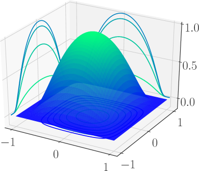
(a) ”Bump” test function

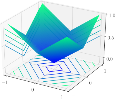
(b) $\|\cdot\|_{1}$ test function

Figure 2: The two test functions

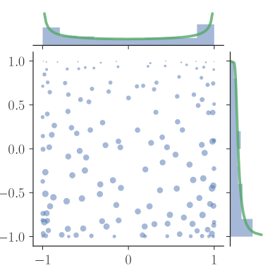
(a) 2D sample

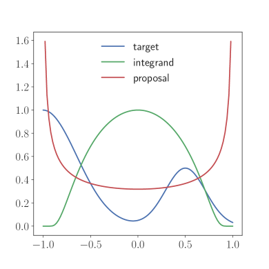
(b) importance sampling setting

Figure 3: 3(a) A weighted sample of the Jacobi OPE described in Section 3.1. 3(b) The test function (3.1) when $d=1$, along with the proposal and the target used for demonstrating the importance sampling procedure in Theorem 4.

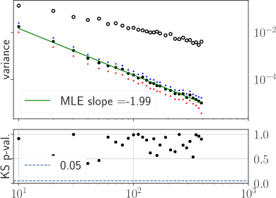
(a) $d=1$

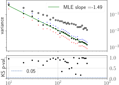
(b) $d=2$

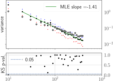
(c) $d=3$

Figure 4: Summary of the crude Monte Carlo results.

For a given dimension $d$, we want to infer the rate of decay of the variance, in order to confirm the rate in the CLT of Theorem 3. We proceed as follows. We first select the values of $N$ for which the $N_{\text{repeat}}$ realizations give a $p$-value larger than $0.05$ in a Kolmogorov-Smirnov test of Gaussianity. This is meant to eliminate the small values of $N$ for which the Gaussian in the CLT (2.21) is a bad approximation for our samples. We do not claim to perform any multiple testing, but rather use the $p$-value as a loose indicator of Gaussianity. The bottom plot of each quadrant of Figure 4 shows the $p$-values as a function of $N$. Note how Gaussianity is hinted even for small $N$ in $d=1,2$, while for $d=3$, it takes larger $N$ to kick in. Then, we perform a standard frequentist linear regression on the selected log variances vs. $\log(N)$. For visualization, we plot on each quadrant of Figure 4 the maximum likelihood (MLE) line in green and indicate its slope in the legend. The usual Student-t confidence intervals for the slope are given in the column of Table 1 labeled Crude MC.

$d$	$-1-1/d$	Crude MC	Importance sampling	Assumption violation
1	$-2$	$[-2.05,-1.92]$	$[-2.13,-1.99]$	$[-2.08,-1.92]$
2	$-1.5$	$[-1.55,-1.43]$	$[-1.61,-1.44]$	$[-1.60,-1.42]$
3	$-1.33$	$[-1.49,-1.33]$	$[-1.42,-1.16]$	$\bf{[-1.24,-1.07]}$

Table 1: Confidence intervals for the variance decay, for all three experiments of Section 3. In bold, we highlight the only confidence interval that does not contain the corresponding theoretical rate given in the second column.

The confidence intervals are in very good agreement with Theorem 3 for each dimension $d$. The combined plots in Figure 4 hint that the CLT approximation is strikingly accurate for all $d$, even for small $N$. For $d=3$, the Gaussianity appears slightly later in terms of $N$, which confirms the intuition that the convergence to a Gaussian is slower when the dimension increases. Relatedly, the intercept of the various straight lines increases with $d$, and this increase seems to be faster for DPPs than crude Monte Carlo. This entails that the value of $N$ above which OPEs becomes significantly more efficient than crude Monte Carlo increases with $d$, as can be seen in Figure 4.

3.3 Importance sampling: illustrating Theorem 4

We now illustrate the importance sampling result in Theorem 4. As proposal reference measure, we use the OPEs described in Section 3.1. More precisely, we take $q(x){\rm d}x$ in Theorem 4 to be the product Jacobi measure described in Section 3.1. The goal is still to estimate the integral of $\varphi$ in (3.1), but this time with respect to a target distribution $\mu$ that is a truncated mixture of two Gaussians, with density

$$\omega(x)=\frac{1}{2}\exp\left[-\frac{\|x-0.5\|^{2}}{(0.3)^{2}}\right]+\exp\left[-\frac{\|x+1\|^{2}}{(0.5)^{2}}\right]$$

with respect to the Lebesgue measure on $I^{d}$. The target measure $\mu$, the proposal reference measure and the test function are illustrated in $d=1$ in Figure 3(b).

For the sake of shortness, we defer the figure displaying the results of the regression to Figure 5 in Appendix D. We only report here the resulting confidence intervals on the rate of decay of the variance, in the column of Table 1 labeled importance sampling. Again, the confidence intervals are in very good agreement with the CLT in Theorem 4.

3.4 An integrand that violates the assumptions of Theorem 3

We again copy the setting of Section 3.1, but we change the integrand to

$$f(x)=d^{-1}\|x\|_{1}.$$

This test function is plotted in Figure 2(b) for $d=2$. It does not belong to the class $\mathscr{C}$ that we authorize in Theorem 3: it is not $\mathscr{C}^{1}$, and it does not vanish at the border of $I^{d}$. Again, we defer the display of the regression to Figure 6 in Appendix D, and we limit ourselves here to the confidence intervals on the slope, which are given in the last column of Table 1. This time, while the decay of the mean square error is still significantly better than crude Monte Carlo, the confidence intervals do not all match the conclusion of Theorem 3: we have written in bold the confidence interval for $d=3$, which suggests a rate of decay that is slower than $-1-1/d$. This is a hint that the assumptions of Theorem 3 are essentially tight.

4 Discussion and perspectives

As detailed in Remark 3, Monte Carlo with DPPs is a stochastic counterpart to Gaussian quadrature, introduced in Section 1.1. Compared to the Monte Carlo methods introduced in Section 1.2, and 1.3, Theorem 4 is an importance sampling procedure, with negatively correlated importance samples. This negative correlation results in a variance reduction that impacts the decay rate of the variance. Loosely speaking, this is reminiscent of the surprising kernel density approach to importance sampling of Delyon and Portier (2016) described in Section 1.2. Our rates are better for equivalent smoothness in $d=1$, but for $d>1$, the theoretical comparison is less clear. In terms of sampling cost, (Delyon and Portier, 2016) scales as $\mathcal{O}(N^{2})$ not taking into account the tuning of the kernel parameters. Naively sampling orthogonal polynomial ensembles is $\mathcal{O}(N^{3})$, without taking rejection sampling into account. Tackling the cubic cost of sampling DPPs is a natural sequel to our work, see also Section 2.4.

Monte Carlo with DPPs is also reminiscent of randomized quasi-Monte Carlo methods such as scrambled nets (Owen, 1997), discussed in Section 1.3. The important difference is that randomness and discrepancy are tied in our DPP proposal. The similarities with QMC are an interesting lead for future research. In particular, fast constructions of nets in QMC (Dick et al., 2013) could yield fast sampling algorithms for DPPs.

Monte Carlo with DPPs also connects with Bayesian quadrature, introduced in Section 1.4. As pointed out in Section 2.4, sampling projection DPPs is related to sequentially maximizing the variance of a Gaussian process, while Bayesian quadrature is about sequentially minimizing the variance of the integral of $f$ when a Gaussian process prior is assumed on $f$, see Section 1.4. A formal connection with Bayesian quadrature would facilitate the transfer of CLTs such as our Theorem 4 to Bayesian quadrature. Conversely, the efficient Frank-Wolfe optimization procedures given for herding by Bach et al. (2012); Briol et al. (2019) could influence fast sampling algorithms for DPPs.

Additionally, theoretical rates have been provided for hybrid integral estimators in (Briol et al., 2015, Theorem 1), which mix classical Monte Carlo nodes with Bayesian quadrature weights, effectively reducing the influence of close-by pairs of Monte Carlo samples. Together with (Delyon and Portier, 2016), the latter approach uses a kernel to introduce anti-correlation in a postprocessing reweighting step. In comparison, Monte Carlo with DPPs also uses a kernel to encode repulsiveness, but the repulsiveness not only appears in the weights: it is embedded in the sampling procedure.

The same reason that sampling and approximation are both encapsulated in the same DPP object is the major difference with the postprocessing approaches of (Oates et al., 2017; Liu and Lee, 2017). With DPPs, we lose the algorithmic simplicity and often low cost of postprocessing, but we gain a CLT with weaker, dimension-independent smoothness requirements. Also, our importance reweighted estimator in Theorem 4 bypasses the need to know the moments of the target measure, which is akin to removing the constraint of knowing the integral of the control approximation to the integrand in (Oates et al., 2017). There are interesting avenues to try to obtain a hybrid algorithm that would get the best of both worlds.

Finally, we comment on our focus on orthogonal polynomials and projection kernels. Relying on orthogonal polynomials made available technology that we extensively used in the proofs, such as precise asymptotic results and the use of recurrence coefficients. First, with slightly stronger estimates, one may allow the reference measure to depend on $N$, so as to replace the equilibrium measure $\mu_{eq}^{\otimes d}$ by a measure putting less mass on the boundary of the integration domain. This would prevent part of the quadrature nodes to clutter close to the boundary of the hypercube. Second, any projection kernel onto an $N$-dimensional subspace of $L^{2}(\mu)$ yields an appropriate DPP for numerical integration, and orthogonal polynomials may not be the most natural choice of basis for a given integrand. It is easy to imagine kernels built on wavelets or other bases of $L^{2}(\mu)$, and a clever choice of basis may also yield faster sampling algorithms, but the difficulty lies in obtaining such variance estimates as we obtained for orthogonal polynomials. Third, one should keep in mind that not every projection kernel leads to small variance. For instance, the projection kernel onto

$$\mathrm{Span}(e^{2ik\pi\theta}:\;k=0,\ldots,N-1)$$

yields a DPP on $[-1,1]$ such that $\mathbb{V}{\mathrm{ar}}[\sum f(\mathbf{x}_{i})]\sim N$ for any odd function of $L^{2}(-1,1)$. On the positive side, extra complex structure can buy us further variance reduction in even dimensions for analytic test functions. For instance, one can show along the lines of Section B.2, that the projection onto $\mathrm{Span}(z^{k}:\;k=0,\ldots,N-1)$ yields a DPP on the unit disc with $\mathbb{V}{\mathrm{ar}}[\sum f(\mathbf{x}_{i})]\sim 1$ instead of $N^{1-1/2}$ provided the function $f$ is analytic. Fourth, one may be tempted to use contraction kernels instead of projection kernels, but besides the problem that the number of points drawn from the DPP becomes random, contraction DPPs are bound to augment the variance of linear statistics.

To conclude, DPPs are a new way to connect numerical integration with rich analytic tools.

Acknowledgments:

AH would like to thank Bernhard Beckermann, Jeff Geronimo and Kurt Johansson for useful and stimulating discussions. This work started while RB and AH were respectively at University of Oxford and KTH Royal Institute of Technology, funded by EPSRC grant number EP/I017909/1 and grant KAW 2010.0063 from the Knut and Alice Wallenberg Foundation. RB also acknowledges support from ANR grant Bnpsi ANR-13-BS03-0006, and AH acknowledges support from Labex CEMPI ANR-11-LABX-0007-01. Finally, both authors acknowledge support from CNRS through PEPS JCJC DppMc and from ANR through grant BoB ANR-16-CE23-0003.

Appendix

Appendix A Preliminary material

In this section, we provide some general background on orthogonal polynomials, we prove short results and we outline the proofs of the main theorems.

A.1 Orthogonal polynomials and the Nevai class

In the following, we use the equilibrium measure $\mu_{eq}$ of $I$, defined by

$$\mu_{eq}({\rm d}x)=\omega_{eq}(x){\rm d}x,\qquad\omega_{eq}(x)=\frac{1}{\pi\sqrt{1-x^{2}}}\ \boldsymbol{1}_{I}(x).$$ (A.1)

The name comes from its characterization as the unique minimizer of the logarithmic energy $\iint\log|x-y|^{-1}\mu({\rm d}x)\mu({\rm d}y)$ over Borel probability measures $\mu$ on $I$ (Saff and Totik, 1997). It is also the image of the uniform measure on the unit circle through the map $e^{i\theta}\mapsto x=\cos\theta$. The associated orthonormal polynomials are the normalized Chebyshev polynomials of the first kind, defined on $I$ by

$$T_{k}(\cos\theta)=\begin{cases}\sqrt{2}\cos(k\theta)&\mbox{if }k\geqslant 1\\ 1&\mbox{if }k=0\end{cases}\;,\qquad\theta\in[0,\pi].$$ (A.2)

They satisfy the three-term recurrence relation

$$xT_{k}(x)=a_{k}^{*}T_{k+1}(x)+b_{k}^{*}T_{k}(x)+a_{k-1}^{*}T_{k-1}(x),\qquad k\in\mathbb{N},$$ (A.3)

where

$$a_{k}^{*}=\begin{cases}0&\mbox{if }k=-1\\ 1/\sqrt{2}&\mbox{if }k=0\\ 1/2&\mbox{if }k\geqslant 1\end{cases}\qquad\mbox{and }\qquad b_{k}^{*}=0.$$ (A.4)

More generally, given a reference measure $\mu$ on $I$ with orthonormal polynomials $(\varphi_{k})$, we always have the three-term recurrence relation

$$x\varphi_{k}(x)=a_{k}\varphi_{k+1}(x)+b_{k}\varphi_{k}(x)+a_{k-1}\varphi_{k-1}(x),\qquad k\in\mathbb{N},$$ (A.5)

where $a_{-1}=0$ and $a_{k}>0$ and $b_{k}\in\mathbb{R}$ for every $k\geqslant 0$. The existence of the recurrence coefficients $(a_{k})_{k\in\mathbb{N}}$ and $(b_{k})_{k\in\mathbb{N}}$ follows by decomposing the polynomial $x\varphi_{k}$ into the orthonormal family $(\varphi_{\ell})_{\ell=0}^{k+1}$ of $L^{2}(\mu)$ and observing that $\langle x\varphi_{k},\varphi_{\ell}\rangle=\langle\varphi_{k},x\varphi_{\ell}\rangle=0$ as soon as $\ell<k-1$ by orthogonality.

Definition 1.

A measure $\mu$ supported on $I$ is Nevai-class if the recurrence coefficients for the associated orthonormal polynomials satisfy

$$\lim_{k\rightarrow\infty}a_{k}=1/2,\qquad\lim_{k\rightarrow\infty}b_{k}=0.$$

Notice the respective limits of the $a_{k}$’s and $b_{k}$’s for Nevai class measures are the recurrence coefficients (A.4) of the measure $\mu_{eq}$ when $k\geqslant 1$.

The next theorem gives a sufficient condition for a measure to be Nevai class (Simon, 2011, Theorem 1.4.2).

Theorem 6.

(Denisov-Rakhmanov) Let $\mu$ be a reference measure on $I$ with Lebesgue decomposition $\mu({\rm d}x)=\omega(x){\rm d}x+\mu_{s}$. If $\omega(x)>0$ almost everywhere, then $\mu$ is Nevai-class.

Consider now the Christoffel-Darboux kernel

$$K_{N}(x,y)=\sum_{k=0}^{N-1}\varphi_{k}(x)\varphi_{k}(y),$$ (A.6)

and notice $\frac{1}{N}K_{N}(x,x)\mu({\rm d}x)$ is a probability measure. One of the interesting properties of Nevai-class measures is that this probability measure has $\mu_{eq}$ for weak limit as $N\to\infty$ (Stahl and Totik, 1992).

Theorem 7.

Assume $\mu$ supported on $I$ is Nevai-class. Then, for every $f\in\mathscr{C}^{0}(I,\mathbb{R})$,

$$\int f(x)\frac{1}{N}K_{N}(x,x)\mu({\rm d}x)\xrightarrow[N\to\infty]{}\int f(x)\mu_{eq}({\rm d}x).$$

Now, consider instead a reference measure $\mu$ on $I^{d}$ with associated multivariate orthogonal polynomials $(\varphi_{k})_{k\in\mathbb{N}}$ (see Section 2.1) and Christoffel-Darboux kernel $K_{N}(x,y)$ defined as in (A.6). Assume further that $\mu=\mu_{1}\otimes\cdots\otimes\mu_{d}$ is a product of $d$ measures $\mu_{j}$ on $I$, and denote by $\varphi_{k}^{(j)}$ and $K_{N}^{(j)}(x,y)$ the respective orthogonal polynomials and Christoffel-Darboux kernel associated with $\mu_{j}$. Then, we have

$$\varphi_{k}(x)=\varphi_{k_{1}}^{(1)}(x_{1})\cdots\varphi_{k_{d}}^{(d)}(x_{d})$$ (A.7)

where $(k_{1},\ldots,k_{d})=\mathfrak{b}(k)$. Moreover,

$$K_{M^{d}}(x,y)=\prod_{j=1}^{d}K_{M}^{(j)}(x_{j},y_{j}).$$ (A.8)

As a consequence, Theorem 7 easily yields the following.

Corollary 1.

Let $\mu=\mu_{1}\otimes\cdots\otimes\mu_{d}$ with $\mu_{j}$ supported on $I$ and Nevai-class. Then, for every $f\in\mathscr{C}^{0}(I^{d},\mathbb{R})$,

$$\int f(x)\frac{1}{N}K_{N}(x,x)\mu({\rm d}x)\xrightarrow[N\to\infty]{}\int f(x)\mu_{eq}^{\otimes d}({\rm d}x).$$ (A.9)

Proof.

By the Stone-Weierstrass theorem, it is enough to show (A.9) when $f(x)=\prod_{j=1}^{d}f_{j}(x_{j})$ with $f_{j}\in\mathscr{C}^{0}(I,\mathbb{R})$. Without loss of generality, one can further assume the functions $f_{j}$ are non-negative. Let $M=\lfloor N^{1/d}\rfloor$ be the unique integer satisfying $M^{d}\leqslant N<(M+1)^{d}$. Since we have $K_{M^{d}}(x,x)\leqslant K_{N}(x,x)\leqslant K_{(M+1)^{d}}(x,x)$ and, by (A.8),

$$\frac{M^{d}}{N}\prod_{j=1}^{d}\int f_{j}(x)\frac{1}{M}K_{M}^{(j)}(x,x)\mu_{j}({\rm d}x)\\ \leqslant\int f(x)\frac{1}{N}K_{N}(x,x)\mu({\rm d}x)\leqslant\frac{(M+1)^{d}}{N}\prod_{j=1}^{d}\int f_{j}(x)\frac{1}{M+1}K_{M+1}^{(j)}(x,x)\mu_{j}({\rm d}x),$$ (A.10)

Corollary 1 follows from Theorem 7. ∎

The next lemma is yet another aspect of Nevai-class measures that is relevant to our proofs, and may be of independent interest.

Lemma 1.

Assume $\mu$ supported on $I$ is Nevai-class. We have the weak convergence of

$$Q_{N}({\rm d}x,{\rm d}y)=(x-y)^{2}K_{N}(x,y)^{2}\mu({\rm d}x)\mu({\rm d}y)$$ (A.11)

towards

$$L({\rm d}x,{\rm d}y)=\frac{1}{2}(1-xy)\mu_{eq}({\rm d}x)\mu_{eq}({\rm d}y).$$ (A.12)

Proof.

First, the Christoffel-Darboux formula reads

$$(x-y)^{2}K_{N}(x,y)^{2}=a_{N}^{2}\big{(}\varphi_{N}(x)\varphi_{N-1}(y)-\varphi_{N-1}(x)\varphi_{N}(y)\big{)}^{2},$$ (A.13)

which follows by computing $xK_{N}(x,y)$ using the recurrence relation (A.5) and witnessing several cancellations when subtracting $yK_{N}(x,y)$. Thus, by the orthonormality conditions, we see $\iint Q_{N}({\rm d}x,{\rm d}y)=2a_{N}^{2}$. Since $\mu$ is Nevai-class, the former converges to $1/2=\iint L({\rm d}x,{\rm d}y)$. This allows us to use the usual weak topology (i.e. the topology coming by duality with respect to the continuous functions) for bounded Borel measures.

Step 1. We first prove the lemma when $\mu=\mu_{eq}$, so that the $\varphi_{k}$’s are the Chebyshev polynomials $T_{k}$, see (A.2). By (A.13), the push-forward of (A.11) by the map $(x,y)\mapsto(\cos\theta,\cos\eta)$, where $\theta,\eta\in[0,\pi]$, reads

$$\frac{1}{\pi^{2}}\big{\{}\cos(N\theta)\cos((N-1)\eta)-\cos((N-1)\theta\cos(N\eta)\big{\}}^{2}{\rm d}\theta{\rm d}\eta.$$ (A.14)

This measure has for Fourier transform

$$\frac{1}{\pi^{2}}\int_{0}^{\pi}\int_{0}^{\pi}e^{i(\theta u+\eta v)}\big{\{}\cos(N\theta)\cos((N-1)\eta)-\cos((N-1)\theta)\cos(N\eta)\big{\}}^{2}{\rm d}\theta{\rm d}\eta\\ =\frac{1}{\pi^{2}}\int_{0}^{\pi}\int_{0}^{\pi}\cos(\theta u+\eta v)\big{\{}\cos(N\theta)\cos((N-1)\eta)-\cos((N-1)\theta)\cos(N\eta)\big{\}}^{2}{\rm d}\theta{\rm d}\eta.$$

By developing the square in the integrand and linearizing the products of cosines, we see that the non-vanishing contribution as $N\to\infty$ of the Fourier transform are the terms which are independent on $N$. Indeed, the $N$-dependent terms come up with a factor $1/N$ after integration. Thus, the Fourier transform equals, up to $\mathcal{O}(1/N)$, to

$$\frac{1}{2\pi^{2}}\int_{0}^{\pi}\int_{0}^{\pi}\cos(\theta u+\eta v)\big{(}1-\cos\theta\cos\eta\big{)}{\rm d}\theta{\rm d}\eta.$$

This yields the weak convergence of (A.14) towards $(2\pi^{2})^{-1}(1-\cos\theta\cos\eta){\rm d}\theta{\rm d}\eta$, and the lemma follows, in the case where $\mu=\mu_{eq}$, by taking the image of the measures by the inverse map $(\cos\theta,\cos\eta)\mapsto(x,y)$.

Step 2. We now prove the lemma for a general Nevai-class measure $\mu$ on $I$. Let us denote by $Q_{N}^{\mu}$ the measure (A.11) in order to stress the dependence on $\mu$. Thanks to Step 1, it is enough to prove that for every $m,n\in\mathbb{N}$, we have

$$\lim_{N\to\infty}\left|\iint x^{m}y^{n}Q_{N}^{\mu}({\rm d}x,{\rm d}y)-\iint x^{m}y^{n}Q_{N}^{\mu_{eq}}({\rm d}x,{\rm d}y)\right|=0,$$

in order to complete the proof of the lemma. Recalling (A.11), (A.13), and that $a_{N}\to 1/2$, it is enough to show that for every $m\in\mathbb{N}$,

$$\lim_{N\to\infty}\left|\int x^{m}\varphi^{2}_{N}(x)\mu({\rm d}x)-\int x^{m}T^{2}_{N}(x)\mu_{eq}({\rm d}x)\right|=0$$ (A.15)

and

$$\lim_{N\to\infty}\left|\int x^{m}\varphi_{N}(x)\varphi_{N-1}(x)\mu({\rm d}x)-\int x^{m}T_{N}(x)T_{N-1}(x)\mu_{eq}({\rm d}x)\right|=0.$$ (A.16)

To do so, we first complete for convenience the sequences of recurrence coefficients $(a_{n})_{n\in\mathbb{N}}$ and $(b_{n})_{n\in\mathbb{N}}$ introduced in (A.5) as bi-infinite sequences $(a_{n})_{n\in\mathbb{Z}}$, $(b_{n})_{n\in\mathbb{Z}}$, where we set $a_{n}=b_{n}=0$ for every $n<0$. It follows inductively from the three-term recurrence relation (A.5) that for every $k,\ell,m\in\mathbb{N}$,

$$\int x^{m}\varphi_{k}(x)\varphi_{\ell}(x)\mu({\rm d}x)=\sum_{\gamma:(0,k)\rightarrow(m,\ell)}\prod_{e\in\gamma}\omega(e)_{\{(a_{n}),\,(b_{n})\}},$$ (A.17)

where the sum ranges over all the paths $\gamma$ lying on the oriented graph with vertices $\mathbb{Z}^{2}$ and edges $(i,j)\to(i+1,j+1)$, $(i,j)\to(i+1,j)$ and $(i,j)\to(i+1,j-1)$ for $(i,j)\in\mathbb{Z}^{2}$, starting from $(0,k)$ and ending at $(m,\ell)$. For every edge $e$ of $\mathbb{Z}^{2}$, we introduced the weight associated with the sequences $(a_{n})=(a_{n})_{n\in\mathbb{Z}}$, $(b_{n})=(b_{n})_{n\in\mathbb{Z}}$ defined by

$$\omega(e)_{\{(a_{n}),\,(b_{n})\}}=\begin{cases}a_{j}&\mbox{if }e=(i,j)\to(i+1,j+1)\\ b_{j}&\mbox{if }e=(i,j)\to(i+1,j)\\ a_{j-1}&\mbox{if }e=(i,j)\to(i+1,j-1),\end{cases}$$ (A.18)

see also (Hardy, 2015). Now, observe that the set of all paths $\gamma$ satisfying $\gamma:(0,k)\rightarrow(m,\ell)$ only depends on $k,\ell$ through $|k-\ell|$ and is empty as soon as $|k-\ell|>m$. Thus it is a finite set, and moreover, by translation of the indices, for every $k,\ell,m\in\mathbb{N}$ we have

$$\int x^{m}\varphi_{k}(x)\varphi_{\ell}(x)\mu({\rm d}x)=\mathbf{1}_{|k-\ell|\leqslant m}\sum_{\gamma:(0,k-\ell)\rightarrow(m,0)}\prod_{e\in\gamma}\omega(e)_{\{(a_{n+\ell}),\,(b_{n+\ell})\}}.$$ (A.19)

In particular, see (A.3)–(A.4),

$$\int x^{m}T_{k}(x)T_{\ell}(x)\mu_{eq}({\rm d}x)=\mathbf{1}_{|k-\ell|\leqslant m}\sum_{\gamma:(0,k-\ell)\rightarrow(m,0)}\prod_{e\in\gamma}\omega(e)_{\{(a^{*}_{n+\ell}),\,(b^{*}_{n+\ell})\}}.$$ (A.20)

Finally, by combining (A.19) and (A.20), we obtain

$$\left|\int x^{m}\varphi_{k}(x)\varphi_{\ell}(x)\mu({\rm d}x)-\int x^{m}T_{k}(x)T_{\ell}(x)\mu_{eq}({\rm d}x)\right|\\ \leqslant\sum_{\gamma:(0,k-\ell)\rightarrow(m,0)}\Big{|}\prod_{e\in\gamma}\omega(e)_{\{(a_{n+\ell}),\,(b_{n+\ell})\}}-\prod_{e\in\gamma}\omega(e)_{\{(a^{*}_{n+\ell}),\,(b^{*}_{n+\ell})\}}\Big{|}.$$ (A.21)

Together with the Nevai-class assumption for $\mu$, which states that $a_{n}-a_{n}^{*}\to 0$ and $b_{n}-b_{n}^{*}\to 0$ as $n\to\infty$, it follows that (A.15) and (A.16) hold true by taking $k=\ell=N$, or $k=N$ and $\ell=N-1$, in (A.21). This completes the proof of Lemma 1.

∎

A.2 Sketch of the proof of Theorem 2

A.2.1 Reduction to probability reference measures

First, in the statement of Theorem 2, we can assume the reference measure $\mu$ is a probability measure without loss of generality. This will simplify notation in the proof of Theorem 2.

Indeed, for any positive measure $\mu$ on $I^{d}$ with (multivariate) orthonormal polynomials $\varphi_{k}$ and any $\alpha>0$, the orthonormal polynomials associated with $\alpha\mu$ are $\varphi_{k}/\sqrt{\alpha}$. Thus, if we momentarily denote by $K_{N}(\mu;x,y)$ the $N$th Christoffel-Darboux kernel associated with a measure $\mu$, we have $K_{N}(\alpha\mu;x,y)=K_{N}(\mu;x,y)/\alpha$. As a consequence, for every $n\geqslant 1$, the correlation measures

$$\det\Big{[}K_{N}(\mu;x_{i},x_{\ell})\Big{]}_{i,\ell=1}^{n}\prod_{i=1}^{n}\mu({\rm d}x_{i}),$$

remain unchanged if we replace $\mu$ by $\alpha\mu$ for any $\alpha>0$. Hence, multivariate OP Ensembles are invariant under $\mu\mapsto\alpha\mu$.

A.2.2 Soshnikov’s key theorem

As stated previously, Theorem 2 has already been proven when $d=1$ by Breuer and Duits (2017), as a consequence of a generalized strong Szegő theorem they obtained. The difficulty in proving Theorem 2 when $d\geqslant 2$ turns out to be of different nature than the one-dimensional setting. Indeed, the next result due to Soshnikov essentially states that the cumulants of order three and more of the linear statistic $\sum f(\mathbf{x}_{i})$ decay to zero as $N\to\infty$ as soon as its variance goes to infinity, and we will show the variance indeed diverges when $d\geqslant 2$. Thus, a CLT follows easily as soon as one can obtain asymptotic estimates on the variance. However, if obtaining such variance estimates is relatively easy when $d=1$, the task becomes more involved in higher dimension.

More precisely, the general result (Soshnikov, 2002, Theorem 1) has the following consequence.

Theorem 8.

(Soshnikov) Let $\mathbf{x}_{1},\ldots,\mathbf{x}_{N}$ form a multivariate OP Ensemble with respect to a given reference measure $\mu$ on $I^{d}$. Consider a sequence $(f_{N})$ of uniformly bounded and measurable real-valued functions on $I^{d}$ satisfying, as $N\to\infty$,

$$\mathbb{V}{\mathrm{ar}}\left[\,\sum_{i=1}^{N}f_{N}(\mathbf{x}_{i})\right]\longrightarrow\infty,$$ (A.22)

and, for some $\delta>0$,

$$\mathbb{E}\left[\,\sum_{i=1}^{N}\big{|}f_{N}(\mathbf{x}_{i})\big{|}\right]=O\left(\mathbb{V}{\mathrm{ar}}\left[\,\sum_{i=1}^{N}f_{N}(\mathbf{x}_{i})\right]^{\delta}\right).$$ (A.23)

Then, we have

$$\frac{\displaystyle\sum_{i=1}^{N}f_{N}(\mathbf{x}_{i})-\mathbb{E}\left[\,\sum_{i=1}^{N}f_{N}(\mathbf{x}_{i})\right]}{\displaystyle\sqrt{\mathbb{V}{\mathrm{ar}}\left[\,\sum_{i=1}^{N}f_{N}(\mathbf{x}_{i})\right]}}\xrightarrow[N\to\infty]{law}\mathcal{N}(0,1).$$

A.2.3 Variance asymptotics

In order to prove Theorem 2 it is enough to show the following asymptotics.

Proposition 3.

Assume $\mu$ and $\mathbf{x}_{1},\ldots,\mathbf{x}_{N}$ satisfy the hypothesis of Theorem 2. Then, for every $f\in\mathscr{C}^{1}(I^{d},\mathbb{R})$, we have

$$\lim_{N\to\infty}\frac{1}{N^{1-1/d}}\mathbb{V}{\mathrm{ar}}\left[\,\sum_{i=1}^{N}f(\mathbf{x}_{i})\right]=\sigma_{f}^{2}.$$ (A.24)

Indeed, for any $d\geqslant 2$ and any $f\in\mathscr{C}^{1}(I^{d},\mathbb{R})$, Corollary 1 and Proposition 3 imply (A.22) and (A.23) with $f_{N}=f$ and $\delta=d/(d-1)$. Thus, we can apply Theorem 8 to obtain Theorem 2.

Proposition 3 is the main technical result of this work. Consider the $d$-fold product of the equilibrium measure (A.1), namely the probability measure on $I^{d}$ given by

$$\mu_{eq}^{\otimes d}({\rm d}x)=\omega_{eq}^{\otimes d}(x){\rm d}x,\qquad\omega_{eq}^{\otimes d}(x)=\prod_{j=1}^{d}\frac{1}{\pi\sqrt{1-x_{j}^{2}}}\ \boldsymbol{1}_{I^{d}}(x).$$ (A.25)

In our proof of Proposition 3, we start by investigating the limit (A.24) when $\mu=\mu_{eq}^{\otimes d}$, since algebraic identities are available for this reference measure. Then, we use comparison estimates to prove (A.24) in the general case.

A.3 A proof for the upper bound on the limiting variance

As stated in Proposition 1, one can bound the limiting variance $\sigma_{f}^{2}$ by a Dirichlet energy. Besides providing some control on the amplitude of $\sigma_{f}^{2}$, we will need this inequality in the proof of Proposition 3. We now give a proof for this proposition.

Proof of Proposition 1.

Let $\mu_{sc}({\rm d}x)=\pi^{-1}\sqrt{1-x^{2}}{\boldsymbol{1}}_{I}(x){\rm d}x$ be the semi-circle measure. The associated orthonormal polynomials are the so-called Chebyshev polynomials of the second kind

$$U_{k}(\cos\theta)=\sqrt{2}\,\frac{\sin((k+1)\theta)}{\sin\theta}.$$

For any $1\leqslant j\leqslant d$, define the measure

$$\nu^{j}({\rm d}x)=\mu_{eq}({\rm d}x_{1})\cdots\mu_{eq}({\rm d}x_{j-1})\mu_{sc}({\rm d}x_{j})\mu_{eq}({\rm d}x_{j+1})\cdots\mu_{eq}({\rm d}x_{d}),$$

so that the RHS of (2.9) becomes

$$\frac{1}{2}\sum_{j=1}^{d}\int_{I^{d}}\Big{(}\partial_{j}f(x)\Big{)}^{2}\,\nu^{j}({\rm d}x).$$

For any $\boldsymbol{k}=(k_{1},\ldots,k_{d})\in\mathbb{N}^{d}$, set $T_{\boldsymbol{k}}(x)=T_{k_{1}}(x_{1})\cdots T_{k_{d}}(x_{d})$, where $T_{k}$ are the Chebyshev polynomials (A.2), and let

$$V_{\boldsymbol{k}}^{j}(x)=T_{k_{1}}(x_{1})\cdots T_{k_{j-1}}(x_{j-1})U_{k_{j}}(x_{j})T_{k_{j+1}}(x_{j+1})\cdots T_{k_{d}}(x_{d}).$$

Thus, $(T_{\boldsymbol{k}})_{\boldsymbol{k}\in\mathbb{N}^{d}}$ and $(V^{j}_{\boldsymbol{k}})_{\boldsymbol{k}\in\mathbb{N}^{d}}$ respectively form an orthonormal Hilbert basis of $L^{2}(\mu_{eq}^{\otimes d})$ and $L^{2}(\nu^{j})$. Let $f\in\mathscr{C}^{1}(I^{d},\mathbb{R})$, so that $f=\sum_{\boldsymbol{k}\in\mathbb{N}^{d}}\hat{f}(\boldsymbol{k})T_{\boldsymbol{k}}$ where $\hat{f}(\boldsymbol{k})$ is as in (2.8). Using the identity $T_{k}^{\prime}=kU_{k-1}$, it comes

$$\partial_{j}f(x)=\sum_{\boldsymbol{k}\in\mathbb{N}^{d}}k_{j}\hat{f}(\boldsymbol{k})V_{\boldsymbol{k}}^{j}(x).$$

Then, Parseval’s identity in $L^{2}(\nu^{j})$ yields

$$\int_{I^{d}}\Big{(}\partial_{j}f(x)\Big{)}^{2}\,\nu^{j}({\rm d}x)=\sum_{\boldsymbol{k}\in\mathbb{N}^{d}}k_{j}^{2}\hat{f}(\boldsymbol{k})^{2}.$$

Summing over $1\leqslant j\leqslant d$, the RHS of (2.9) equals

$$\frac{1}{2}\sum_{j=1}^{d}\int_{I^{d}}\Big{(}\partial_{j}f(x)\Big{)}^{2}\,\nu^{j}({\rm d}x)=\frac{1}{2}\sum_{\boldsymbol{k}\in\mathbb{N}^{d}}(k_{1}^{2}+\,\cdots\,+k_{d}^{2})\hat{f}({\boldsymbol{k}})^{2},$$ (A.26)

from which Proposition 1 easily follows.

∎

A.4 Assumptions of Theorem 3 and outline of the proof

We now discuss the assumptions and proof of Theorem 3.

Assume the reference measure $\mu$ is a product of $d$ measures on $I$, and also that $\mu$ has a density $\omega$. Then, Corollary 1 suggests that, as $N\to\infty$,

$$\frac{N}{K_{N}(x,x)}\approx\frac{\omega(x)}{\omega_{eq}^{\otimes d}(x)}.$$ (A.27)

This heuristic would yield for the variance of the estimator (2.11),

$$\mathbb{V}{\mathrm{ar}}\left[\ \sum_{i=1}^{N}\frac{f(\mathbf{x}_{i})}{K_{N}(\mathbf{x}_{i},\mathbf{x}_{i})}\ \right]\approx\frac{1}{N^{2}}\mathbb{V}{\mathrm{ar}}\left[\ \sum_{i=1}^{N}f(\mathbf{x}_{j})\frac{\omega(\mathbf{x}_{j})}{\omega_{eq}^{\otimes d}(\mathbf{x}_{j})}\ \right]\approx\frac{\Omega_{f,\omega}^{2}}{N^{1+1/d}}\ ,$$ (A.28)

where for the last approximation we used Proposition 3 with test function $f\omega/\omega_{eq}^{\otimes d}$, recalling $\Omega_{f,\omega}$ was defined in (2.17). This would essentially yield the CLT in Theorem 3 by applying Theorem 8 to $f_{N}(x)=Nf(x)/K_{N}(x,x)$. To make the approximation (A.28) rigorous, we will need extra regularity assumptions on $\mu$.

First, regarding the approximation (A.27), we have the following result.

Theorem 9.

(Totik) Assume $\mu({\rm d}x)=\omega(x){\rm d}x$ with $\omega(x)=\omega_{1}(x_{1})\cdots\omega_{d}(x_{d})$, and that $\omega_{j}$ is continuous and positive on $I$. Then, for every $\varepsilon>0$, we have

$$\frac{N}{K_{N}(x,x)}\xrightarrow[N\to\infty]{}\frac{\omega(x)}{\omega_{eq}(x)}$$ (A.29)

uniformly for $x\in I^{d}_{\varepsilon}$.

For a proof of Theorem 9 when $d=1$, see (Simon, 2011, Section 3.11) and references therein. The case $d\geqslant 2$ follows by the same arguments as in the proof of Corollary 1.

Remark 7.

It is because of Theorem 9 that we restrict $\mathscr{C}^{1}(I^{d},\mathbb{R})$ to the class $\mathscr{C}$ defined in (2.13) in the assumptions of Theorem 3. Unfortunately, there are examples of reference measures $\mu$ on $I$ such that the convergence (A.29) is not uniform on the whole of $I$. However, in order to extend $\mathscr{C}$ to $\mathscr{C}^{1}(I^{d},\mathbb{R})$ in the statement of Theorem 3, it would be enough to have $\sup_{x\in I^{d}_{\varepsilon_{N}}}|N/K_{N}(x,x)-\omega(x)/\omega_{eq}^{\otimes d}(x)|\to 0$ for some sequence $\varepsilon_{N}$ going to zero as $N\to\infty$, but we were not able to locate such a result in the literature.

Next, the first approximation in (A.28) requires a control on the rate of change of $N/K_{N}(x,x)$. To this end, we introduce an extra assumption on the reference measure $\mu$. More precisely, let us denote

$$\mathscr{D}_{N}(x,y)=\frac{N/K_{N}(x,x)-N/K_{N}(y,y)}{\|x-y\|},$$ (A.30)

and further consider the sequence of measures on $I^{d}\times I^{d}$

$$Q_{N}({\rm d}x,{\rm d}y)=\frac{1}{N^{1-1/d}}\|x-y\|^{2}K_{N}(x,y)^{2}\mu({\rm d}x)\mu({\rm d}y).$$ (A.31)

Our extra assumption on $\mu$ is then the following.

Assumption 1.

The measure $\mu$ satisfies

$$\lim_{C\to\infty}\limsup_{\delta\to 0}\limsup_{N\to\infty}\iint_{I^{d}_{\varepsilon}\times I^{d}_{\varepsilon},\ \|x-y\|\leqslant\delta}\mathbf{1}_{\left|\mathscr{D}_{N}(x,y)\right|>C}\ \mathscr{D}_{N}(x,y)^{2}\ Q_{N}({\rm d}x,{\rm d}y)=0.$$ (A.32)

In plain words, this means the squared rate of change $\mathscr{D}_{N}(x,y)^{2}$ is uniformly integrable with respect to the measures $Q_{N}$, at least on the restricted domain where $\|x-y\|$ is small enough and where $x$ and $y$ are not allowed to reach the boundary of $I^{d}$.

Remark 8.

When $d=1$, Lemma 1 states that if $\mu$ is Nevai-class then $Q_{N}$ converges weakly as $N\to\infty$ towards

$$L({\rm d}x,{\rm d}y)=\frac{1}{2\pi^{2}}\frac{1-xy}{\sqrt{1-x^{2}}\sqrt{1-y^{2}}}\ \boldsymbol{1}_{I\times I}(x,y){\rm d}x{\rm d}y.$$

Because the density of $L$ is smooth within $I_{\varepsilon}\times I_{\varepsilon}$ for every $\varepsilon>0$, one may at least heuristically understand that (A.32) reduces to the uniform integrability of $\mathscr{D}_{N}(x,y)^{2}$ with respect to the Lebesgue measure instead. In higher dimension, a similar guess can be made, but we do not pursue this reasoning here.

We now discuss sufficient conditions for (A.32) to hold true.

Remark 9.

Since, for any $\kappa>0$, we have

$$\mathbf{1}_{\left|\mathscr{D}_{N}(x,y)\right|>C}\ \mathscr{D}_{N}(x,y)^{2}\leqslant\frac{1}{C^{\kappa}}\left|\mathscr{D}_{N}(x,y)\right|^{2+\kappa},$$

we see that condition (A.32) holds true as soon as, for every $\varepsilon>0$, there exists $\kappa,\delta>0$ satisfying

$$\limsup_{N\to\infty}\iint_{I^{d}_{\varepsilon}\times I^{d}_{\varepsilon},\ \|x-y\|\leqslant\delta}\left|\mathscr{D}_{N}(x,y)\right|^{2+\kappa}\ Q_{N}({\rm d}x,{\rm d}y)<\infty.$$

Namely, condition (A.32) is satisfied if the $L^{2+\kappa}(Q_{N})$ norm of the rate of change of $N/K_{N}(x,x)$ is bounded, at least on the restricted domain where $\|x-y\|$ is small enough and $x,y$ away from the boundary of $I^{d}$.

The following assumption, which appears in Theorems 3 to 5, is much stronger than Assumption 1, but it is easier to check in practice.

Assumption 2.

The measure $\mu$ satisfies

• $\mu({\rm d}x)=\omega(x){\rm d}x$ with $\omega$ positive and continuous on $(-1,1)^{d}$.

• For every $\varepsilon>0$, the sequence

  $$\frac{1}{N}\sup_{x\in I_{\varepsilon}^{d}}\Big{\|}\nabla K_{N}(x,x)\Big{\|}$$

  is bounded.

Indeed, thanks to the rough upper bound

$$|\mathscr{D}_{N}(x,y)|\leqslant\sup_{x\in I_{\varepsilon}^{d}}\left\|\nabla(N/K_{N}(x,x))\right\|,\qquad x,y\in\boldsymbol{1}_{I_{\varepsilon}^{d}},$$

we see that Assumption 1 holds true as soon as for every $\varepsilon>0$, $\sup_{x\in I_{\varepsilon}^{d}}\|\nabla(N/K_{N}(x,x))\|$ is bounded. Under Assumption 2(a), the latter follows from Assumption 2(b). Indeed, Theorem 9 and Assumption 2(a) together yield that for every $\varepsilon>0$, there exists $c>0$ independent of $N$ such that $\frac{1}{N}K_{N}(x,x)>c$ for every $x\in I_{\varepsilon}^{d}$.

We conclude this section by proving that Jacobi measures (2.18) satisfy Assumption 2, which proves our Proposition 2. We start with a general lemma.

Lemma 2.

Assume the measures $\mu_{1},\dots,\mu_{d}$ on $I$ satisfy Assumption 2. Then the measure $\mu_{1}\otimes\dots\otimes\mu_{d}$ on $I^{d}$ satisfies Assumption 2.

Proof.

We decompose the set $\Gamma_{N}=\{\mathfrak{b}(0),\ldots,\mathfrak{b}(N-1)\}\subset\mathbb{N}^{d}$ in a convenient way. To do so, set $\sigma_{j}(\boldsymbol{k})=(k_{1},\ldots,k_{j-1},k_{j+1},\ldots,k_{d})$ and say that $\boldsymbol{k}\sim\boldsymbol{\ell}$ if and only if $\sigma_{j}(\boldsymbol{k})=\sigma_{j}(\boldsymbol{\ell})$, that is, they have same coordinates except maybe the $j$th one. We denote by $[\boldsymbol{k}]$ the equivalence class under this relation. Set $N_{j}([\boldsymbol{k}])=\max\{\ell_{j}:\boldsymbol{\ell}\in[\boldsymbol{k}]\cap\Gamma_{N}\}$. Using the notation introduced in (A.7) and (A.8), it comes

$$\partial_{j}K_{N}(x,x) =2\sum_{\boldsymbol{k}=\mathfrak{b}(0)}^{\mathfrak{b}(N-1)}\varphi_{k_{j}}^{(j)}(x_{j})\frac{{\rm d}}{{\rm d}x_{j}}\varphi_{k_{j}}^{(j)}(x_{j})\prod_{\alpha\neq j}\varphi_{k_{\alpha}}^{(\alpha)}(x_{\alpha})^{2}$$

$$=2\sum_{[\boldsymbol{k}]\in\Gamma_{N}/\sim}\;\prod_{\alpha\neq j}\varphi^{(\alpha)}_{k_{\alpha}}(x_{\alpha})^{2}\sum_{k_{j}=0}^{N_{j}([\boldsymbol{k}])}\varphi_{k_{j}}^{(j)}(x_{j})\frac{{\rm d}}{{\rm d}x_{j}}\varphi_{k_{j}}^{(j)}(x_{j})$$

$$=\sum_{[\boldsymbol{k}]\in\Gamma_{N}/\sim}\;\prod_{\alpha\neq j}\varphi^{(\alpha)}_{k_{\alpha}}(x_{\alpha})^{2}\,\frac{{\rm d}}{{\rm d}x_{j}}\left[K^{(j)}_{N_{j}([\boldsymbol{k}])+1}(x_{j},x_{j})\right].$$ (A.33)

Let now $\varepsilon>0$. Since $\mu_{j}$ satisfies Assumption 2, there exists $C>0$ such that for all $x\in I_{\varepsilon}$ and $n\in\mathbb{N}$,

$$\left|\frac{{\rm d}}{{\rm d}x}\left[K^{(j)}_{n}(x,x)\right]\right|\leqslant Cn.$$

Let $M=\lfloor N^{1/d}\rfloor$, so that $\Gamma_{N}\subset\mathcal{C}_{M+1}$, see (2.6). Thus, $N_{j}([\boldsymbol{k}])\leqslant M$ for all $\boldsymbol{k}\in\Gamma_{N}$. By (A.33),

$$\left|\partial_{j}K_{N}(x,x)\right| \leqslant C(M+1)\sum_{[\boldsymbol{k}]\in\Gamma_{N}/\sim}\;\prod_{\alpha\neq j}\varphi^{(\alpha)}_{k_{\alpha}}(x_{\alpha})^{2}$$

$$\leqslant C(M+1)\sum_{[\boldsymbol{k}]\in\mathcal{C}_{M+1}}\;\prod_{\alpha\neq j}\varphi^{(\alpha)}_{k_{\alpha}}(x_{\alpha})^{2}$$

$$= C(M+1)\prod_{\alpha\neq j}K_{M+1}^{(\alpha)}(x_{\alpha},x_{\alpha}).$$

Hence

$$\frac{1}{N}\left|\partial_{j}K_{N}(x,x)\right|\leqslant C\frac{M+1}{M}\prod_{\alpha\neq j}\frac{1}{M}K_{M+1}^{(\alpha)}(x_{\alpha},x_{\alpha}),$$

and the lemma follows with Theorem 9. ∎

Lemma 3.

Let $\alpha,\beta>-1$, then the measure

$$(1-x)^{\alpha}(1+x)^{\beta}{\boldsymbol{1}}_{I}(x){\rm d}x$$

satisfies Assumption 2.

Proof.

Let $\varepsilon>0$ be fixed. For convenience, Section A.2.1 allows us to work with the probability measure

$$\mu^{(\alpha,\beta)}({\rm d}x)=\omega^{(\alpha,\beta)}(x){\rm d}x,\qquad\omega^{(\alpha,\beta)}(x)=\frac{1}{c_{\alpha,\beta}}(1-x)^{\alpha}(1+x)^{\beta},$$

where the normalization constant reads

$$c_{\alpha,\beta}=2^{\alpha+\beta+1}\frac{\Gamma(\alpha+1)\Gamma(\beta+1)}{\Gamma(\alpha+\beta+1)}$$

and $\Gamma$ is the Euler Gamma function.

Denote by $(\varphi_{n}^{(\alpha,\beta)})_{n\in\mathbb{N}}$ the associated orthonormal polynomials. They satisfy

$$\varphi_{n}^{(\alpha,\beta)}(x)=\frac{P_{n}^{(\alpha,\beta)}(x)}{\sqrt{h_{n}^{(\alpha,\beta)}}},$$

where the $P_{n}^{(\alpha,\beta)}$’s are the Jacobi polynomials (we refer to (Szegő, 1974) for definitions and properties) and

$$h_{n}^{(\alpha,\beta)}=\|P_{n}^{(\alpha,\beta)}\|^{2}_{L^{2}(\mu^{(\alpha,\beta)})}=\frac{1}{n!(\alpha+\beta+2n+1)}\frac{\Gamma(\alpha+\beta+1)\Gamma(\alpha+n+1)\Gamma(\beta+n+1)}{\Gamma(\alpha+1)\Gamma(\beta+1)\Gamma(\alpha+\beta+n+1)},$$

and moreover

$$(\varphi_{n}^{(\alpha,\beta)})^{\prime}=\frac{u_{\alpha,\beta}}{2}\sqrt{n(n+\alpha+\beta+1)}\ \varphi_{n-1}^{(\alpha+1,\beta+1)},\qquad u_{\alpha,\beta}=\sqrt{\frac{(\alpha+\beta+1)(\alpha+\beta+2)}{(\alpha+1)(\beta+1)}}.$$ (A.34)

This yields

$$\frac{{\rm d}}{{\rm d}x}K_{N}(x,x) =2\sum_{k=1}^{N-1}\varphi_{k}^{(\alpha,\beta)}(x)(\varphi_{k}^{(\alpha,\beta)})^{\prime}(x)$$

$$=u_{\alpha,\beta}\sum_{k=1}^{N-1}\sqrt{k(k+\alpha+\beta+1)}\ \varphi_{k}^{(\alpha,\beta)}(x)\varphi_{k-1}^{(\alpha+1,\beta+1)}(x).$$ (A.35)

By (Kuijlaars et al., 2004), we have as $k\to\infty$, uniformly in $x=\cos\theta\in I_{\varepsilon}$,

$$\varphi_{k}^{(\alpha,\beta)}(\cos\theta)=\sqrt{\frac{2}{\omega^{(\alpha,\beta)}(x)\pi\sqrt{1-x^{2}}}}\ \cos\left(\big{(}k+\frac{1}{2}(\alpha+\beta+1)\big{)}\theta-\frac{\pi}{2}(\alpha+\frac{1}{2})\right)+O(1/k).$$ (A.36)

As a consequence, we obtain in the same asymptotic regime,

$$\varphi_{k-1}^{(\alpha+1,\beta+1)}(\cos\theta)=\sqrt{\frac{2}{\omega^{(\alpha,\beta)}(x)\pi\sqrt{1-x^{2}}}}\ \sin\left(\big{(}k+\frac{1}{2}(\alpha+\beta+1)\big{)}\theta-\frac{\pi}{2}(\alpha+\frac{1}{2})\right)+O(1/k).$$ (A.37)

Now (A.36) implies that the $P_{k}^{(\alpha,\beta)}(x)$’s are bounded uniformly for $x\in I$ and $k\in\mathbb{N}$. Using moreover that $2\sin(u)\cos(u)=\sin(2u)$ and combining (A.4)–(A.37), we obtain for some $C_{1},C_{2}>0$ that

$$\sup_{x\in I_{\varepsilon}}\left|\frac{{\rm d}}{{\rm d}x}K_{N}(x,x)\right|\leqslant C_{1}\sup_{x\in I_{\varepsilon}}\left|\sum_{k=1}^{N-1}k\sin\left(\big{(}2k+\alpha+\beta+1\big{)}\theta-\pi(\alpha+\frac{1}{2})\right)\right|+C_{2}$$

where we recall the relation $x=\cos\theta$. Next, we write

$$\left|\sum_{k=1}^{N-1}k\sin\left(\big{(}2k+\alpha+\beta+1\big{)}\theta-\pi(\alpha+\frac{1}{2})\right)\right|\leqslant\left|\sum_{k=1}^{N-1}ke^{i((2k+\alpha+\beta+1)\theta-\pi(\alpha+\frac{1}{2}))}\right|^{1/2}$$

and then

$$\sum_{k=1}^{N-1}ke^{i((2k+\alpha+\beta+1)\theta-\pi(\alpha+\frac{1}{2}))} =e^{i((\alpha+\beta+1)\theta-\pi(\alpha+\frac{1}{2}))}\sum_{k=1}^{N-1}ke^{2ik\theta}$$

$$=\frac{1}{2i}e^{i((\alpha+\beta+1)\theta-\pi(\alpha+\frac{1}{2}))}\frac{{\rm d}}{{\rm d}\theta}\sum_{k=0}^{N-1}e^{2ik\theta}$$

$$=\frac{1}{2i}e^{i((\alpha+\beta+1)\theta-\pi(\alpha+\frac{1}{2}))}\frac{{\rm d}}{{\rm d}\theta}\Big{(}\frac{e^{i(N-1)\theta}\sin(N\theta)}{\sin(\theta)}\Big{)}.$$ (A.38)

Since the absolute value of the right hand side of (A.4) is bounded by $CN/\sin^{2}(\theta)$ for some $C>0$ independent on $N$ and $\theta$, the lemma follows.

∎

Lemmas 2 and 3 combined yield Proposition 2.

A.5 Proof of Theorem 5

Proof of Theorem 5.

We proceed in two steps. The first step is to prove a bivariate CLT for the vector $(\mathscr{I}_{N}(f),\mathscr{I}_{N}(1))$, and the second step is to apply the delta method to obtain a central limit theorem for the ratio.

Let $t,v\in\mathbb{R}$. We apply Theorem 4 to $tf+vh$, where $h$ is any function in $\mathscr{C}$ that is equal to $1$ on $I_{\varepsilon}^{d}$. This leads to

$$\sqrt{N^{1+1/d}}\left(t\mathscr{I}_{N}(f)+v\mathscr{I}_{N}(1)-t\int f\omega_{u}{\rm d}x-vZ\right)\rightarrow\mathcal{N}(0,Z^{2}\Omega_{tf+vh,\omega}^{2}),$$

where

$$\Omega_{tf+vh,\omega}^{2}=t^{2}\Omega_{f,\omega}^{2}+v^{2}\Omega_{1,\omega}^{2}+2tvc_{f,\omega}.$$

By the Crámer-Wold theorem (Kallenberg, 2006, Corollary 5.5), we obtain a bivariate CLT

$$\sqrt{N^{1+1/d}}\left[\begin{pmatrix}\mathscr{I}_{N}(f)\\ \mathscr{I}_{N}(1)\end{pmatrix}-\begin{pmatrix}\int f\omega_{u}{\rm d}x\\ Z\end{pmatrix}\right]\rightarrow\mathcal{N}\left(0,Z^{2}\begin{pmatrix}\Omega_{f,\omega}^{2}&c_{f,\omega}\\ c_{f,\omega}&\Omega_{1,\omega}^{2}\end{pmatrix}\right).$$

Now we apply the delta method (Schervish, 2012, Section 7.1.3) to obtain

$$\sqrt{N^{1+1/d}}\left[\frac{\mathscr{I}_{N}(f)}{\mathscr{I}_{N}(1)}-\int f{\rm d}\mu\right]\rightarrow\mathcal{N}\left(0,Z^{2}\begin{pmatrix}\frac{1}{Z}&-\frac{\int f\omega_{u}{\rm d}x}{Z^{2}}\end{pmatrix}\begin{pmatrix}\Omega_{f,\omega}^{2}&c_{f,\omega}\\ c_{f,\omega}&\Omega_{1,\omega}^{2}\end{pmatrix}\begin{pmatrix}\frac{1}{Z}\\ -\frac{\int f\omega_{u}{\rm d}x}{Z^{2}}\end{pmatrix}\right),$$

which is precisely (2.22). ∎

Appendix B CLT for multivariate OP Ensembles: proof of Theorem 2

In this section we prove Proposition 3. As explained in Section A.2, Theorem 2 follows from this proposition.

B.1 A useful representation of the covariance

Lemma 4.

Let $\mathbf{x}_{1},\ldots,\mathbf{x}_{N}$ be random variables drawn from a multivariate OP Ensemble with reference measure $\mu$. For any multivariate polynomials $P,Q$, we have

$$\mathbb{C}{\rm ov}\left[\,\sum_{i=1}^{N}P(\mathbf{x}_{i}),\sum_{i=1}^{N}Q(\mathbf{x}_{i})\right]=\sum_{n=0}^{N-1}\sum_{m=N}^{\infty}\langle P\varphi_{n},\varphi_{m}\rangle\langle Q\varphi_{n},\varphi_{m}\rangle,$$

where $\langle\,\cdot\,,\,\cdot\,\rangle$ refers to the scalar product of $L^{2}(\mu)$.

Proof.

We start from the standard formula

$$\mathbb{C}{\rm ov}\left[\,\sum_{i=1}^{N}P(\mathbf{x}_{i}),\sum_{j=1}^{N}Q(\mathbf{x}_{i})\right]\\ =\int P(x)Q(x)K_{N}(x,x)\mu({\rm d}x)-\iint P(x)Q(y)K_{N}(x,y)^{2}\mu({\rm d}x)\mu({\rm d}y),$$ (B.1)

which follows from (2.1)–(2.3) with $n=1,2$ and that $K_{N}(x,y)$ is symmetric. On the one hand, it follows from the definition of $K_{N}$ that

$$\iint P(x)Q(y)K_{N}(x,y)^{2}\mu({\rm d}x)\mu({\rm d}y)=\sum_{n=0}^{N-1}\sum_{m=0}^{N-1}\langle P\varphi_{n},\varphi_{m}\rangle\langle Q\varphi_{n},\varphi_{m}\rangle.$$ (B.2)

On the other hand, by using the decomposition (where the sum is finite since $P$ is polynomial)

$$P\varphi_{n}=\sum_{m=0}^{\infty}\langle P\varphi_{n},\varphi_{m}\rangle\varphi_{m}$$

together with the identity

$$\int P(x)Q(x)K_{N}(x,x)\mu({\rm d}x)=\sum_{n=0}^{N-1}\langle P\varphi_{n},Q\varphi_{n}\rangle,$$

we obtain

$$\int P(x)Q(x)K_{N}(x,x)\mu({\rm d}x)=\sum_{n=0}^{N-1}\sum_{m=0}^{\infty}\langle P\varphi_{n},\varphi_{m}\rangle\langle Q\varphi_{n},\varphi_{m}\rangle.$$ (B.3)

Lemma 4 then follows by combining (B.1), (B.2) and (B.3). ∎

B.2 Covariance asymptotics: the Chebyshev case

We first investigate the case of the product measure $\mu^{\otimes d}_{eq}$, where $\mu_{eq}$ defined in (A.1) is the equilibrium measure of $I$. Recalling the definition (A.2), the multivariate Chebyshev polynomials

$$T_{\boldsymbol{k}}(x_{1},\ldots,x_{d})=T_{k_{1}}(x_{1})\cdots T_{k_{d}}(x_{d}),\qquad\boldsymbol{k}=(k_{1},\ldots k_{d})\in\mathbb{N}^{d},$$ (B.4)

satisfy the orthonormality conditions

$$\int T_{\boldsymbol{k}}(x)T_{\boldsymbol{\ell}}(x)\mu_{eq}^{\otimes d}({\rm d}x)=\delta_{\boldsymbol{k}\boldsymbol{\ell}},\qquad\boldsymbol{k},\boldsymbol{\ell}\in\mathbb{N}^{d}.$$

We shall see that the family $(T_{\boldsymbol{k}})_{\boldsymbol{k}\in\mathbb{N}^{d}}$ diagonalizes the covariance structure associated with our point process.

Proposition 4.

Let $\mathbf{x}_{1}^{*},\ldots,\mathbf{x}_{N}^{*}$ be drawn according to the multivariate OP Ensemble associated with $\mu_{eq}^{\otimes d}$. Then, given any multi-indices $\boldsymbol{k}=(k_{1},\ldots,k_{d})\in\mathbb{N}^{d}$ and $\boldsymbol{\ell}=(\ell_{1},\ldots,\ell_{d})\in\mathbb{N}^{d}$, we have

$$\lim_{N\rightarrow\infty}\frac{1}{N^{1-1/d}}\,\mathbb{C}{\rm ov}\left[\,\sum_{i=1}^{N}T_{\boldsymbol{k}}(\mathbf{x}_{i}^{*}),\sum_{i=1}^{N}T_{\boldsymbol{\ell}}(\mathbf{x}_{i}^{*})\right]=\begin{cases}\displaystyle\frac{1}{2}(k_{1}+\,\cdots\,+k_{d})&\mbox{if }\boldsymbol{k}=\boldsymbol{\ell},\\ \displaystyle 0&\mbox{if }\boldsymbol{k}\neq\boldsymbol{\ell}.\end{cases}$$

As a warm-up, let us first prove the proposition when $d=1$.

Proof of Proposition 4 when $d=1$.

Throughout this proof, $\langle\cdot,\cdot\rangle$ denotes the inner product in $L^{2}(\mu_{eq}^{\otimes d})$. For every $k,\ell\in\mathbb{N}$, Lemma 4 provides

$$\mathbb{C}{\rm ov}\left[\,\sum_{i=1}^{N}T_{k}(\mathbf{x}_{i}^{*}),\sum_{i=1}^{N}T_{\ell}(\mathbf{x}_{i}^{*})\right]=\sum_{n=0}^{N-1}\sum_{m=N}^{\infty}\langle T_{k}T_{n},T_{m}\rangle\langle T_{\ell}T_{n},T_{m}\rangle.$$ (B.5)

First, notice that if $k$ or $\ell$ is zero, then the right-hand side of (B.5) vanishes because $\langle T_{n},T_{m}\rangle=\delta_{nm}$, and hence we can assume both $k,\ell$ are non-zero. Next, (A.2) yields the multiplication formula

$$T_{k}T_{n}=\frac{1}{\sqrt{2}}\,T_{n+k}\,\mathbf{1}_{kn\neq 0}+\left(\frac{1}{\sqrt{2}}\right)^{\mathbf{1}_{nk\neq 0}\mathbf{1}_{n\neq k}}T_{|n-k|},\qquad k,n\in\mathbb{N}.$$ (B.6)

Combined with the orthonormality relations, this yields for any $n,m\in\mathbb{N}$ and $k>0$

$$\langle T_{k}T_{n},T_{m}\rangle\\ =\frac{1}{\sqrt{2}}\,\boldsymbol{1}_{n+k=m}\boldsymbol{1}_{n\neq 0}+\left(\frac{1}{\sqrt{2}}\right)^{\boldsymbol{1}_{n\neq 0}\boldsymbol{1}_{n\neq k}}\boldsymbol{1}_{|n-k|=m}.$$ (B.7)

Hence, if $n,m\in\mathbb{N}$ moreover satisfy $n<m$ and $m>\max(k,\ell)$, then we have

$$\langle T_{k}T_{n},T_{m}\rangle\langle T_{\ell}T_{n},T_{m}\rangle=\frac{1}{2}\boldsymbol{1}_{n\neq 0}\boldsymbol{1}_{n+k=m}\boldsymbol{1}_{\ell+n=m}.$$ (B.8)

By plugging (B.8) into (B.5), we obtain for every $N>\max(k,\ell)$,

$$\mathbb{C}{\rm ov}\left[\,\sum_{i=1}^{N}T_{k}(\mathbf{x}_{i}^{*}),\sum_{i=1}^{N}T_{\ell}(\mathbf{x}_{i}^{*})\right] =\frac{1}{2}\sum_{n=1}^{N-1}\sum_{m=N}^{\infty}\boldsymbol{1}_{k+n=m}\boldsymbol{1}_{\ell+n=m}$$

$$=\frac{1}{2}k\,\boldsymbol{1}_{k=\ell},$$

and the proposition follows when $d=1$. ∎

We now provide a proof for the higher-dimensional case. We also use the multiplication formula (B.6) in an essential way, although the setting is more involved. We recall that we introduced the bijection $\mathfrak{b}:\mathbb{N}\to\mathbb{N}^{d}$ associated with the graded lexicographic order in Section 2.1.3.

Proof of Proposition 4 when $d\geqslant 2$.

Fix multi-indices $\boldsymbol{k}=(k_{1},\ldots,k_{d})\in\mathbb{N}^{d}$ and $\boldsymbol{\ell}=(\ell_{1},\ldots,\ell_{d})\in\mathbb{N}^{d}$, and also set

$$S=\big{\{}j:\;k_{j}\neq 0\big{\}},\qquad S^{\prime}=\big{\{}j:\;\ell_{j}\neq 0\big{\}}.$$

Thanks to Lemma 4, we can write

$$\mathbb{C}{\rm ov}\left[\,\sum_{i=1}^{N}T_{\boldsymbol{k}}(\mathbf{x}_{i}^{*}),\sum_{i=1}^{N}T_{\boldsymbol{\ell}}(\mathbf{x}_{i}^{*})\right]=\sum_{(\boldsymbol{n},\boldsymbol{m})\in\mathbb{A}_{N}}\langle T_{\boldsymbol{k}}T_{\boldsymbol{n}},T_{\boldsymbol{m}}\rangle\langle T_{\boldsymbol{\ell}}T_{\boldsymbol{n}},T_{\boldsymbol{m}}\rangle,$$ (B.9)

where we introduced for convenience the set

$$\mathbb{A}_{N}=\Big{\{}(\boldsymbol{n},\boldsymbol{m})\in\mathbb{N}^{d}\times\mathbb{N}^{d}:\quad\boldsymbol{n}\leqslant\mathfrak{b}(N-1),\quad\boldsymbol{m}\geqslant\mathfrak{b}(N)\Big{\}}.$$ (B.10)

Next, using (B.4), the orthonormality relations for the Chebyshev polynomials and (B.7), we obtain

$$\langle T_{\boldsymbol{k}}T_{\boldsymbol{n}},T_{\boldsymbol{m}}\rangle= \;\;\langle T_{k_{1}}T_{n_{1}},T_{m_{1}}\rangle_{L^{2}(\mu_{eq})}\cdots\langle T_{k_{d}}T_{n_{d}},T_{m_{d}}\rangle_{L^{2}(\mu_{eq})}$$ (B.11)

$$\;= \quad\Big{(}\prod_{j\notin S}\mathbf{1}_{n_{j}=m_{j}}\Big{)}\sum_{P\subset S}\left(\frac{1}{\sqrt{2}}\right)^{|P|+|\{j\in S\setminus P:\;n_{j}\neq 0,\,n_{j}\neq k_{j}\}|}$$

$$\times\Big{(}\prod_{j\in P}\mathbf{1}_{n_{j}+k_{j}=m_{j}}\mathbf{1}_{n_{j}\neq 0}\Big{)}\Big{(}\prod_{j\in S\setminus P}\mathbf{1}_{|n_{j}-k_{j}|=m_{j}}\Big{)},$$ (B.12)

where $|A|$ stands for the cardinality of the set $A$.

First, notice that if $S\neq S^{\prime}$ then the right hand side of (B.9) vanishes. Indeed, if $S\neq S^{\prime}$, then there exists $\alpha\in\{1,\ldots,d\}$ such that $k_{\alpha}=0$ and $\ell_{\alpha}\neq 0$ (or the other way around, but the argument is symmetric). It then follows from (B.12) that $\langle T_{\boldsymbol{k}}T_{\boldsymbol{n}},T_{\boldsymbol{m}}\rangle$ vanishes except if $n_{\alpha}=m_{\alpha}$, and moreover that $\langle T_{\boldsymbol{\ell}}T_{\boldsymbol{n}},T_{\boldsymbol{m}}\rangle$ vanishes except if $|n_{\alpha}\pm\ell_{\alpha}|=m_{\alpha}$. Since $\ell_{\alpha}\neq 0$, it holds $\langle T_{\boldsymbol{k}}T_{\boldsymbol{n}},T_{\boldsymbol{m}}\rangle\langle T_{\boldsymbol{\ell}}T_{\boldsymbol{n}},T_{\boldsymbol{m}}\rangle=0$ for every $(\boldsymbol{n},\boldsymbol{m})\in\mathbb{N}^{d}\times\mathbb{N}^{d}$, and our claim follows. Moreover, because $(\boldsymbol{n},\boldsymbol{m})\in\mathbb{A}_{N}$ yields the existence of $\alpha\in\{1,\ldots,d\}$ such that $n_{\alpha}<m_{\alpha}$, one can see from (B.11) that $\langle T_{\boldsymbol{k}}T_{\boldsymbol{n}},T_{\boldsymbol{m}}\rangle$ vanishes for every $(\boldsymbol{n},\boldsymbol{m})\in\mathbb{A}_{N}$ if $\boldsymbol{k}=(0,\ldots,0)$. We henceforth assume that $S=S^{\prime}\neq\varnothing$, for the covariance not to be trivial.

By combining (B.9) with (B.12), we obtain

$$\mathbb{C}{\rm ov}\left[\,\sum_{i=1}^{N}T_{\boldsymbol{k}}(\mathbf{x}_{i}^{*}),\sum_{i=1}^{N}T_{\boldsymbol{\ell}}(\mathbf{x}_{i}^{*})\right]=\sum_{P,Q\subset S}\sum_{(\boldsymbol{n},\boldsymbol{m})\in\mathbb{A}_{N}[P,Q]}\left(\frac{1}{\sqrt{2}}\right)^{\sigma[P,Q](\boldsymbol{n})},$$

where we introduced the subsets

$$\mathbb{A}_{N}[P,Q]=\Bigg{\{}(\boldsymbol{n},\boldsymbol{m})\in\mathbb{A}_{N}\;\Bigg{|}\;\begin{matrix}n_{j}+k_{j}=m_{j},\\ n_{j}+\ell_{j}=m_{j},\end{matrix}\quad\begin{matrix}n_{j}\neq 0,\\ n_{j}\neq 0,\end{matrix}\quad\begin{matrix}\mbox{ if }j\in P\\ \mbox{ if }j\in Q\end{matrix}\;;\\ \begin{matrix}|n_{j}-k_{j}|=m_{j},\\ |n_{j}-\ell_{j}|=m_{j},\end{matrix}\quad\begin{matrix}\mbox{ if }j\in S\setminus P\\ \mbox{ if }j\in S\setminus Q\end{matrix}\;;\qquad n_{j}=m_{j},\quad\mbox{ if }j\notin S\;\Bigg{\}}$$ (B.13)

and set for convenience

$$\sigma[P,Q](\boldsymbol{n})=|P|+|Q|+|\big{\{}j\in S\setminus P:\;n_{j}\neq 0,\,n_{j}\neq k_{j}\big{\}}|\\ +|\big{\{}j\in S\setminus Q:\;n_{j}\neq 0,\,n_{j}\neq\ell_{j}\big{\}}|.$$ (B.14)

Notice from (B.13) if $k_{\alpha}=\ell_{\alpha}\neq 0$ and $\mathbb{A}_{N}[P,Q]\neq\varnothing$ then necessarily $\alpha\in P\cap Q$ or $\alpha\in(S\setminus P)\cap(S\setminus Q)$. In particular, if $\boldsymbol{k}=\boldsymbol{\ell}$ then $\mathbb{A}_{N}[P,Q]=\varnothing$ unless $P=Q$. Thus,

$$\mathbb{C}{\rm ov}\left[\,\sum_{i=1}^{N}T_{\boldsymbol{k}}(\mathbf{x}_{i}^{*}),\sum_{i=1}^{N}T_{\boldsymbol{\ell}}(\mathbf{x}_{i}^{*})\right]=\boldsymbol{1}_{\boldsymbol{k}\,=\,\boldsymbol{\ell}}\sum_{P\subset S}\sum_{(\boldsymbol{n},\boldsymbol{m})\in\mathbb{A}_{N}[P,P]}\left(\frac{1}{\sqrt{2}}\right)^{\sigma[P,P](\boldsymbol{n})}\\ +\boldsymbol{1}_{\boldsymbol{k}\,\neq\,\boldsymbol{\ell}}\sum_{P,Q\subset S}\sum_{(\boldsymbol{n},\boldsymbol{m})\in\mathbb{A}_{N}[P,Q]}\left(\frac{1}{\sqrt{2}}\right)^{\sigma[P,Q](\boldsymbol{n})}.$$ (B.15)

Our goal is now to show that for every $P,Q\subset S$ the following holds true. As $N\to\infty$, if we assume $\boldsymbol{k}=\boldsymbol{\ell}$, then

$$\sum_{(\boldsymbol{n},\boldsymbol{m})\in\mathbb{A}_{N}[P,P]}\left(\frac{1}{\sqrt{2}}\right)^{\sigma[P,P](\boldsymbol{n})}=\left(\frac{1}{2}\right)^{|S|}\Big{(}\sum_{j\in P}k_{j}\Big{)}N^{1-1/d}+o(N^{1-1/d}),$$ (B.16)

and, if instead $\boldsymbol{k}\neq\boldsymbol{\ell}$, then

$$\big{|}\mathbb{A}_{N}[P,Q]\big{|}=o(N^{1-1/d}).$$ (B.17)

Since an easy rearrangement argument together with the definition of $S$ yield

$$\sum_{P\subset S}\Big{(}\sum_{j\in P}k_{j}\Big{)} =\frac{1}{2}\sum_{P\subset S}\Big{(}\sum_{j\in S}k_{j}\Big{)}$$

$$=\Big{(}\sum_{j\subset S}k_{j}\Big{)}2^{|S|-1}=\Big{(}\sum_{j=1}^{d}k_{j}\Big{)}2^{|S|-1},$$

Proposition 4 would then follow from (B.15)–(B.17).

We now turn to the proof of (B.16) and (B.17).

Truncated sets and consequences.

Given distinct $\alpha_{1},\ldots,\alpha_{p}\in\{1,\ldots,d\}$, we introduce the truncated sets

$$\mathbb{A}_{N}[P,Q;\alpha_{1},\ldots,\alpha_{p}]\\ =\mathbb{A}_{N}[P,Q]\cap\big{\{}n_{\alpha_{1}}\leqslant\max(k_{\alpha_{1}},\ell_{\alpha_{1}})\big{\}}\cap\,\cdots\,\cap\big{\{}n_{\alpha_{p}}\leqslant\max(k_{\alpha_{p}},\ell_{\alpha_{p}})\big{\}}.$$ (B.18)

By definition of $\mathfrak{b}$ and $\mathbb{A}_{N}$, if $N=M^{d}$ then $\mathbb{A}_{M^{d}}=\mathcal{C}_{M}\times(\mathbb{N}^{d}\setminus\mathcal{C}_{M})$ where we recall

$$\mathcal{C}_{M}=\Big{\{}\boldsymbol{n}\in\mathbb{N}^{d}:\;0\leqslant n_{1},\ldots,n_{d}\leqslant M-1\Big{\}}.$$ (B.19)

Moreover, if for an arbitrary $N$ we denote by $M=\lfloor N^{1/d}\rfloor$ the integer satisfying $M^{d}\leqslant N<(M+1)^{d}$, then $\mathfrak{b}(N)\in\mathcal{C}_{M+1}$ and thus, for any $(\boldsymbol{n},\boldsymbol{m})\in\mathbb{A}_{N}$, we have $\boldsymbol{n}\in\mathcal{C}_{M+1}$. As a consequence, for every $P,Q\subset S$, we have the rough upper bound $|\mathbb{A}_{N}[P,Q;\alpha_{1},\ldots,\alpha_{p}]|=\mathcal{O}(M^{d-p})$. In particular,

$$\big{|}\mathbb{A}_{N}[P,Q;\alpha_{1},\ldots,\alpha_{p}]\big{|}=o(N^{1-1/d})\quad\mbox{ for every }p\geqslant 2.$$ (B.20)

In order to restrict ourselves to the easier setting where $N$ is a power of $d$, we will use the following lemma. Its proof uses in a crucial way the graded lexicographic order we chose to equip $\mathbb{N}^{d}$ with, and it is deferred to the end of the present proof.

Lemma 5.

Assume $\boldsymbol{k}=\boldsymbol{\ell}$. For every $P\subset S$, $\alpha\in S\setminus P$ and for every $N>\max(k_{1}^{d},\ldots,k_{d}^{d})$, we have

• $\big{|}\mathbb{A}_{N}[P,P]\big{|}\leqslant\big{|}\mathbb{A}_{N+1}[P,P]\big{|}$,
  

• $\big{|}\mathbb{A}_{N}[P,P;\alpha]\big{|}\leqslant\big{|}\mathbb{A}_{N+1}[P,P;\alpha]\big{|}$.

Proof of (B.16).

Assume $\boldsymbol{k}=\boldsymbol{\ell}$. As a consequence of Lemma 5 (a), if we set $M=\lfloor N^{1/d}\rfloor$ then we have for every $N$ large enough

$$\sum_{(\boldsymbol{n},\boldsymbol{m})\in\mathbb{A}_{M^{d}}[P,P]}\left(\frac{1}{\sqrt{2}}\right)^{\sigma[P,P](\boldsymbol{n})} \leqslant\sum_{(\boldsymbol{n},\boldsymbol{m})\in\mathbb{A}_{N}[P,P]}\left(\frac{1}{\sqrt{2}}\right)^{\sigma[P,P](\boldsymbol{n})}\leqslant\sum_{(\boldsymbol{n},\boldsymbol{m})\in\mathbb{A}_{(M+1)^{d}}[P,P]}\left(\frac{1}{\sqrt{2}}\right)^{\sigma[P,P](\boldsymbol{n})}.$$

Thus, it is enough to prove that, as $M\to\infty$,

$$\sum_{(\boldsymbol{n},\boldsymbol{m})\in\mathbb{A}_{M^{d}}[P,P]}\left(\frac{1}{\sqrt{2}}\right)^{\sigma[P,P](\boldsymbol{n})}=\left(\frac{1}{2}\right)^{|S|}\Big{(}\sum_{j\in P}k_{j}\Big{)}M^{d-1}+o(M^{d-1}),$$ (B.21)

in order to establish (B.16). To do so, for any $P\subset S$ and $\alpha\in S\setminus P$, we set

$$\mathbb{A}_{M^{d}}^{*}[P] =\mathbb{A}_{M^{d}}[P,P]\cap\big{\{}n_{j}>k_{j}\mbox{ for all }j\in S\setminus P\big{\}},$$ (B.22)

$$\mathbb{A}_{M^{d}}^{*}[P;\alpha] =\mathbb{A}_{M^{d}}[P,P;\alpha]\cap\big{\{}n_{j}>k_{j}\mbox{ for all }j\in S\setminus(P\cup\{\alpha\})\big{\}},$$ (B.23)

and use the following lemma; its proof is deferred to the end of the actual proof.

Lemma 6.

Assume $\boldsymbol{k}=\boldsymbol{\ell}$. For every $P\subset S$ and $\alpha\in S\setminus P$, we have as $M\to\infty$

$$\big{|}\mathbb{A}_{M^{d}}^{*}[P]\big{|} =\Big{(}\sum_{j\in P}k_{j}\Big{)}M^{d-1}+o(M^{d-1}),$$ (B.24)

$$\big{|}\mathbb{A}_{M^{d}}^{*}[P;\alpha]\big{|} =o(M^{d-1}).$$ (B.25)

Next, as a consequence of the rough upper bound (B.20) and (B.25), we can write

$$\big{|}\mathbb{A}_{M^{d}}[P,P]\big{|}= \;\big{|}\mathbb{A}_{M^{d}}[P,P]\cap\big{\{}n_{\alpha}>k_{\alpha}\mbox{ for all }\alpha\in S\setminus P\big{\}}\big{|}$$

$$+\big{|}\mathbb{A}_{M^{d}}[P,P]\cap\big{\{}n_{\alpha}\leqslant k_{\alpha}\mbox{ for at least one }\alpha\in S\setminus P\big{\}}\big{|}$$

$$= \;\big{|}\mathbb{A}^{*}_{M^{d}}[P]\big{|}+\sum_{\alpha\in S\setminus P}\big{|}\mathbb{A}^{*}_{M^{d}}[P;\alpha]\big{|}+o(M^{d-1})$$

$$= \;\big{|}\mathbb{A}^{*}_{M^{d}}[P]\big{|}+o(M^{d-1}).$$ (B.26)

Since for any $(\boldsymbol{n},\boldsymbol{m})\in\mathbb{A}^{*}_{M^{d}}[P]$ we have $\sigma[P,P](\boldsymbol{n})=2|S|$, see (B.14) and (B.22), the estimate (B.21) follows from (B.2) and (B.24), and the proof of (B.16) is therefore complete.

Proof of (B.17).

Assume now that $\boldsymbol{k}\neq\boldsymbol{\ell}$. Since $\boldsymbol{k}$ and $\boldsymbol{\ell}$ have the same zero components, it follows that neither $k_{\alpha}$ nor $\ell_{\alpha}$ is zero. Thus, (B.13) yields that if $k_{\alpha}\neq\ell_{\alpha}$ and $\mathbb{A}_{N}[P,Q]\neq\varnothing$, then either $\alpha\in P\cap(S\setminus Q)$ or $\alpha\in Q\cap(S\setminus P)$ and moreover, for any $(\boldsymbol{n},\boldsymbol{m})\in\mathbb{A}_{N}[P,Q]$, we have

$$2n_{\alpha}=|k_{\alpha}-\ell_{\alpha}|,\qquad 2m_{\alpha}=k_{\alpha}+\ell_{\alpha}.$$

In particular $\mathbb{A}_{M^{d}}[P,Q]=\mathbb{A}_{M^{d}}[P,Q;\alpha]$. Thus, by virtue of the rough upper bound (B.20), we can assume in the proof of (B.17) that $\boldsymbol{k}$ and $\boldsymbol{\ell}$ differ by exactly one coordinate, namely there exists $\alpha\in\{1,\ldots,d\}$ such that $k_{\alpha}\neq\ell_{\alpha}$ and $k_{j}=\ell_{j}$ for every $j\neq\alpha$. In this setting, $\mathbb{A}_{N}[P,Q]\neq\varnothing$ then yields $P\setminus\{\alpha\}=Q\setminus\{\alpha\}$ and, if $(\boldsymbol{n},\boldsymbol{m})\in\mathbb{A}_{N}[P,Q]$, then $(n_{\alpha},m_{\alpha})$ satisfies the equations

$$\begin{cases}n_{\alpha}+k_{\alpha}=m_{\alpha},\qquad\ell_{\alpha}-n_{\alpha}=m_{\alpha},\qquad n_{\alpha}\neq 0,\qquad\mbox{ if }\alpha\in P\\ n_{\alpha}+\ell_{\alpha}=m_{\alpha},\qquad k_{\alpha}-n_{\alpha}=m_{\alpha},\qquad n_{\alpha}\neq 0,\qquad\mbox{ if }\alpha\in Q\end{cases}.$$

By weakening these constraints to

$$\begin{cases}|\ell_{\alpha}-n_{\alpha}|=m_{\alpha},\qquad n_{\alpha}\leqslant\ell_{\alpha},\qquad\mbox{ if }\alpha\in P\\ |k_{\alpha}-n_{\alpha}|=m_{\alpha},\qquad n_{\alpha}\leqslant k_{\alpha},\qquad\mbox{ if }\alpha\in Q\end{cases},$$

we obtain the upper bound

$$\big{|}\mathbb{A}_{N}[P,Q]\big{|}\leqslant\begin{cases}\big{|}\mathbb{A}_{N}^{(\boldsymbol{\ell},\boldsymbol{\ell})}[Q,Q;\alpha]\big{|}&\mbox{ if }\alpha\in P\\ \big{|}\mathbb{A}_{N}^{(\boldsymbol{k},\boldsymbol{k})}[P,P;\alpha]\big{|}&\mbox{ if }\alpha\in Q\end{cases}$$ (B.27)

where $\mathbb{A}_{N}^{(\boldsymbol{k},\boldsymbol{\ell})}[P,Q;\alpha]$ is defined as in (B.13),(B.18) but we emphasized the multi-indices $\boldsymbol{k},\boldsymbol{\ell}$ which are involved. By setting $M=\lfloor N^{1/d}\rfloor+1$, we obtain from Lemma 5 (b), the rough upper bound (B.20) and (B.23),(B.25) that, as $N\to\infty$,

$$\big{|}\mathbb{A}_{N}^{(\boldsymbol{k},\boldsymbol{k})}[P,P;\alpha]\big{|}$$

$$\qquad\leqslant\;\big{|}\mathbb{A}_{M^{d}}^{(\boldsymbol{k},\boldsymbol{k})}[P,P;\alpha]\big{|}$$

$$\qquad=\;\big{|}\mathbb{A}_{M^{d}}^{(\boldsymbol{k},\boldsymbol{k})}[P,P;\alpha]\cap\big{\{}n_{j}>k_{j}\mbox{ for all }j\in S\setminus(P\cup\{\alpha\})\big{\}}\big{|}+o(N^{1-1/d})$$

$$\qquad=\;\quad o(N^{1-1/d}),$$ (B.28)

and similarly

$$\big{|}\mathbb{A}_{N}^{(\boldsymbol{\ell},\boldsymbol{\ell})}[Q,Q;\alpha]\big{|}=o(N^{1-1/d}).$$ (B.29)

By combining (B.27)–(B.29), we have finally proved (B.17) and the proof of Proposition 4 is thus complete, up to the proof of Lemmas 5 and 6. ∎

We now provide proofs for the remaining lemmas.

Proof of Lemma 5.

Let $(\boldsymbol{n},\boldsymbol{m})\in\mathbb{A}_{N}[P,P]$. Then $(\boldsymbol{n},\boldsymbol{m})\notin\mathbb{A}_{N+1}[P,P]$ if and only if $\boldsymbol{m}=\mathfrak{b}(N)$. Since $\mathfrak{b}(N)\in\mathcal{C}_{M+1}\setminus\mathcal{C}_{M}$, where $M=\lfloor N^{1/d}\rfloor$ and $\mathcal{C}_{M}$ has been introduced in (B.19), there exists $j\in\{1,\ldots,d\}$ such that $\mathfrak{b}(N)_{j}=M$; let $j_{*}$ be the smallest $j$ satisfying this property. Notice also $\boldsymbol{n}\in\mathcal{C}_{M+1}$ and $\boldsymbol{m}\in\mathbb{N}^{d}\setminus\mathcal{C}_{M}$. As soon as $M>\max(k_{1},\ldots,k_{d})$, that we assume from now, the equality $\boldsymbol{m}=\mathfrak{b}(N)$ can only happen if $j_{*}\notin S\setminus P$. Indeed, if $j_{*}\in S\setminus P$, then $m_{{j_{*}}}=|n_{{j_{*}}}-k_{{j_{*}}}|\leqslant\max(n_{{j_{*}}}-1,k_{j_{*}})\leqslant M-1$. As a consequence,

$$\big{|}\mathbb{A}_{N}[P,P]\big{|}\leqslant\big{|}\mathbb{A}_{N+1}[P,P]\big{|}\quad\mbox{ if }{j_{*}}\in S\setminus P.$$

Next, assume that ${j_{*}}\in P$ or ${j_{*}}\notin S$. We claim that if we set

$$\tilde{m}_{j}=\begin{cases}m_{j}+k_{j}&\mbox{ if }j\in P,\\ |m_{j}-k_{j}|&\mbox{ if }j\in S\setminus P,\\ m_{j}&\mbox{ if }j\notin S,\end{cases}$$ (B.30)

then $(\boldsymbol{m},\tilde{\boldsymbol{m}})\in\mathbb{A}_{N+1}[P,P]\setminus\mathbb{A}_{N}[P,P]$. This would show in particular that

$$\big{|}\mathbb{A}_{N}[P,P]\big{|}\leqslant\big{|}\mathbb{A}_{N+1}[P,P]\big{|}\quad\mbox{ if either }{j_{*}}\in P\mbox{ or }{j_{*}}\notin S,$$

and thus complete the proof of (a). That $(\boldsymbol{m},\tilde{\boldsymbol{m}})\in\mathbb{A}_{N+1}[P,P]\setminus\mathbb{A}_{N}[P,P]$ is by construction obvious provided one can show $\tilde{\boldsymbol{m}}\geqslant\mathfrak{b}(N+1)$.

If ${j_{*}}\in P$, then we have

$$\tilde{m}_{j_{*}}=m_{j_{*}}+k_{j_{*}}=M+k_{j_{*}}>M$$

and thus $\tilde{\boldsymbol{m}}\in\mathbb{N}^{d}\setminus\mathcal{C}_{M+1}$. As a consequence, there exists $m\geqslant(M+1)^{d}$ such that $\tilde{\boldsymbol{m}}=\mathfrak{b}(m)$ and, since $N+1\leqslant(M+1)^{d}$, we have shown $\tilde{\boldsymbol{m}}\geqslant\mathfrak{b}(N+1)$.

If ${j_{*}}\notin S$, we argue by contradiction and assume $\tilde{\boldsymbol{m}}\leqslant\mathfrak{b}(N)=\boldsymbol{m}$. We shall see this is not compatible with the graded lexicographic order. Indeed, since by construction $\tilde{\boldsymbol{m}}\neq\boldsymbol{m}$ and $\boldsymbol{n}\neq\boldsymbol{m}$ (because $\boldsymbol{k}\neq(0,\ldots,0)$ by assumption), we actually have $\tilde{\boldsymbol{m}}<\boldsymbol{m}$ and $\boldsymbol{n}<\boldsymbol{m}$. Because ${j_{*}}\notin S$ by assumption, we moreover have $n_{j_{*}}=m_{j_{*}}=\tilde{m}_{j_{*}}=M$ and thus $\boldsymbol{n},\boldsymbol{m},\tilde{\boldsymbol{m}}\in\mathcal{C}_{M+1}\setminus\mathcal{C}_{M}$. As a consequence, ${\boldsymbol{n}}<_{{\rm lex}}\boldsymbol{m}$ and $\tilde{\boldsymbol{m}}<_{{\rm lex}}\boldsymbol{m}$ in the lexicographic order. This means there exists $\gamma\in\{1,\ldots,d\}$ such that $n_{i}=m_{i}$ for every $i<\gamma$ and $n_{\gamma}<m_{\gamma}$, and equivalently $i\notin S$ when $i<\gamma$ and $\gamma\in P$. Similarly, there exists $\eta\in\{1,\ldots,d\}$ such that $\tilde{m}_{i}=m_{i}$ for every $i<\eta$ and $\tilde{m}_{\eta}<m_{\eta}$, and thus $i\notin S$ when $i<\eta$ and $\eta\in S\setminus P$. But this is impossible and thus $\tilde{\boldsymbol{m}}\geqslant\mathfrak{b}(N+1)$, which completes the proof of (a).

Part (b) is proved by following the exact same line of arguments; in this setting one should also check that if $(\boldsymbol{n},\boldsymbol{m})\in\mathbb{A}_{N}[P,P;\alpha]$ then $m_{\alpha}\leqslant k_{\alpha}$ in order to show $(\boldsymbol{m},\tilde{\boldsymbol{m}})$ (with $\tilde{\boldsymbol{m}}$ defined in (B.30)) actually belongs to $\mathbb{A}_{N+1}[P,P;\alpha]$. Recalling $\alpha\in S\setminus P$ by assumption this is clear, indeed $m_{\alpha}=|n_{\alpha}-k_{\alpha}|$ together with $n_{\alpha}\leqslant k_{\alpha}$ yield $m_{\alpha}=k_{\alpha}-n_{\alpha}\leqslant k_{\alpha}$. ∎

Proof of Lemma 6.

To prove (a), fix $P\subset S$ and assume $M>\max(k_{1},\ldots,k_{d})$. It follows from the definitions (B.13),(B.22) that

$$\mathbb{A}_{M^{d}}^{*}[P]=\Bigg{\{}(\boldsymbol{n},\boldsymbol{m})\in\mathbb{A}_{M^{d}}\;\Bigg{|}\;\begin{matrix}[r]n_{j}+k_{j}=m_{j},\\ n_{j}-k_{j}=m_{j},\\ n_{j}=m_{j},\\ \end{matrix}\qquad\begin{matrix}[l]n_{j}\neq 0,\\ n_{j}>k_{j},\\ \\ \end{matrix}\qquad\begin{matrix}[l]\mbox{ if }j\in P\\ \mbox{ if }j\in S\setminus P\\ \mbox{ if }j\notin S\end{matrix}\Bigg{\}}.$$ (B.31)

Recall that $\mathbb{A}_{M^{d}}=\mathcal{C}_{M}\times(\mathbb{N}^{d}\setminus\mathcal{C}_{M})$ where $\mathcal{C}_{M}$ is defined in (B.19). Clearly, if we set

$$\mathcal{C}_{M}[P]=\Big{\{}\boldsymbol{n}\in\mathcal{C}_{M}:\mbox{ there exists $\boldsymbol{m}\in\mathbb{N}^{d}\setminus\mathcal{C}_{M}$},\;(\boldsymbol{n},\boldsymbol{m})\in\mathbb{A}_{M^{d}}^{*}[P]\Big{\}}$$ (B.32)

then $(\boldsymbol{n},\boldsymbol{m})\mapsto\boldsymbol{n}$ is a bijection from $\mathbb{A}_{M^{d}}^{*}[P]$ to $\mathcal{C}_{M}[P]$.

We claim that if for any $p\in P$ we set

$$\mathcal{C}_{M}^{(p)}[P]=\Bigg{\{}\boldsymbol{n}\in\mathcal{C}_{M}\;\Bigg{|}\;\begin{matrix}[r]1\leqslant n_{j}\leqslant M-1\\ k_{j}<n_{j}\leqslant M-1\\ M-k_{p}\leqslant n_{p}\leqslant M-1\end{matrix}\;\begin{matrix}[l]\mbox{ if }j\in P\\ \mbox{ if }j\in S\setminus P\\ \\ \end{matrix}\;\Bigg{\}},$$ (B.33)

then we have

$$\mathcal{C}_{M}[P]=\bigcup_{p\in P}\mathcal{C}_{M}^{(p)}[P].$$ (B.34)

Indeed, let $\boldsymbol{n}\in\mathcal{C}_{M}[P]$. By definition there exists $\boldsymbol{m}\in\mathbb{N}^{d}\setminus\mathcal{C}_{M}$ such that $(\boldsymbol{n},\boldsymbol{m})\in\mathbb{A}_{M^{d}}^{*}[P]$. This provides, see (B.31), that $1\leqslant n_{j}\leqslant M-1$ if $j\in P$, that $k_{j}<n_{j}\leqslant M-1$ if $j\in S\setminus P$, and the existence of $p\in\{1,\ldots,d\}$ satisfying $m_{p}\geqslant M$. Since $\boldsymbol{n}\in\mathcal{C}_{M}$ then $n_{p}\leqslant M-1$ and thus $p\in P$ because otherwise $m_{p}\leqslant n_{p}$. Together with the equation $n_{p}+k_{p}=m_{p}$ this finally yields that $M-k_{p}\leqslant n_{p}\leqslant M-1$, namely $\boldsymbol{n}\in\mathcal{C}_{M}^{(p)}[P]$ for some $p\in P$. As for the reverse inclusion, if $\boldsymbol{n}\in\mathcal{C}_{M}^{(\alpha)}[P]$ for some $\alpha\in P$ then set

$$m_{j}=\begin{cases}n_{j}+k_{j}&\mbox{ if }j\in P,\\ n_{j}-k_{j}&\mbox{ if }j\in S\setminus P,\\ n_{j}&\mbox{ if }j\notin S,\end{cases}$$

and observe that $\boldsymbol{m}\in\mathbb{N}^{d}\setminus\mathcal{C}_{M}$ since $m_{p}\geqslant M$ and $n_{j}-k_{j}\geqslant 0$ for every $j\in S\setminus P$. Thus, since clearly $(\boldsymbol{n},\boldsymbol{m})\in\mathbb{A}_{M^{d}}^{*}[P]$, we have shown $\boldsymbol{n}\in\mathcal{C}_{M}[P]$ and (B.34) is proved.

Next, since for every distinct $p_{1},\ldots,p_{q}\in P$ the definition (B.33) yields

$$\big{|}\mathcal{C}_{M}^{(p_{1})}[P]\cap\,\cdots\,\cap\mathcal{C}_{M}^{(p_{q})}[P]\big{|}=k_{p_{1}}\cdots k_{p_{q}}M^{d-q}+\mathcal{O}(M^{d-q-1}),$$

then (a) follows from (B.34) and the inclusion-exclusion principle.

We now turn to (b) and fix $\alpha\in S\setminus P$. Let $\mathcal{C}_{M}^{(d)}$ be the $d$-dimensional discrete hypercube of length $M$ defined as in (B.19). We then set

$$\mathbb{A}^{(d-1)}_{M^{d-1}}=\mathcal{C}_{M}^{(d-1)}\times(\mathbb{N}^{d-1}\setminus\mathcal{C}_{M}^{(d-1)})$$

and introduce

$$\mathbb{A}_{M^{d-1}}^{*}[P]^{(d-1)}=\Bigg{\{}(\boldsymbol{n},\boldsymbol{m})\in\mathbb{A}^{(d-1)}_{M^{d-1}}\;\Bigg{|}\;\begin{matrix}[r]n_{j}+k_{j}=m_{j},\\ n_{j}-k_{j}=m_{j},\\ n_{j}=m_{j},\\ \end{matrix}\qquad\begin{matrix}[l]n_{j}\neq 0,\\ n_{j}>k_{j},\\ \\ \end{matrix}\qquad\begin{matrix}[l]\mbox{ if }j\in P\\ \mbox{ if }j\in S\setminus(P\cup\{\alpha\})\\ \mbox{ if }j\notin S\setminus\{\alpha\}\end{matrix}\Bigg{\}}.$$

The statement (a) of the lemma applied in dimension $d-1$ then provides

$$\big{|}\mathbb{A}_{M^{d-1}}^{*}[P]^{(d-1)}\big{|}=o(M^{d-1}).$$ (B.35)

Consider the map $\mathfrak{p}:\mathbb{N}^{d}\to\mathbb{N}^{d-1}$ defined by

$$\mathfrak{p}(n_{1},\ldots,n_{d})=(n_{1},\ldots,n_{\alpha-1},n_{\alpha+1},\ldots,n_{d}).$$

Let $(\boldsymbol{n},\boldsymbol{m})\in\mathbb{A}_{M^{d}}^{*}[P;\alpha]$. Since $\boldsymbol{m}\in\mathbb{N}^{d}\setminus\mathcal{C}_{M}^{(d)}$ and $m_{\alpha}\leqslant k_{\alpha}<M$, there exists $j\neq\alpha$ such that $m_{j}\geqslant M$. It follows that $(\mathfrak{p}(\boldsymbol{n}),\mathfrak{p}(\boldsymbol{m}))\in\mathcal{C}_{M}^{(d-1)}\times(\mathbb{N}^{d-1}\setminus\mathcal{C}_{M}^{(d-1)})$ and thus $(\mathfrak{p}(\boldsymbol{n}),\mathfrak{p}(\boldsymbol{m}))\in\mathbb{A}^{*}_{M^{d-1}}[P]^{(d-1)}$. As a consequence, we have the upper bound

$$\big{|}A_{M^{d}}^{*}[P;\alpha]\big{|}\leqslant k_{\alpha}\big{|}(\mathfrak{p}\times\mathfrak{p})\big{(}A_{M^{d}}^{*}[P;\alpha]\big{)}\big{|}\leqslant k_{\alpha}\big{|}A_{M^{d-1}}^{*}[P]^{(d-1)}\big{|}$$

and thus (b) follows from (B.35).

∎

B.3 Covariance asymptotics: the general case

We now extend Proposition 4 to the general setting of measures satisfying the assumptions of Theorem 2. More precisely, we prove the following.

Proposition 5.

Let $\mu=\mu_{1}\otimes\cdots\otimes\mu_{d}$, where the $\mu_{j}$’s are Nevai-class probability measures on $I$. Let $\mathbf{x}_{1},\ldots,\mathbf{x}_{N}$ and $\mathbf{x}_{1}^{*},\ldots,\mathbf{x}_{N}^{*}$ be random variables drawn from the multivariate OP Ensembles with respective reference measures $\mu$ and $\mu_{eq}^{\otimes d}$. Then, given any polynomial functions $P,Q$ on $\mathbb{R}^{d}$,

$$\lim_{N\rightarrow\infty}\frac{1}{N^{1-1/d}}\,\Bigg{|}\,\mathbb{C}{\rm ov}\left[\,\sum_{i=1}^{N}P(\mathbf{x}_{i}),\sum_{j=1}^{N}Q(\mathbf{x}_{i})\right]-\mathbb{C}{\rm ov}\left[\,\sum_{i=1}^{N}P(\mathbf{x}_{i}^{*}),\sum_{j=1}^{N}Q(\mathbf{x}_{i}^{*})\right]\Bigg{|}=0.$$ (B.36)

For the proof of the proposition, we use a few ingredients from the Step 2 of the proof of Lemma 1 to which we refer the reader to.

Proof of Proposition 5.

By linearity, it is enough to prove the proposition with $P(x)=x_{1}^{\alpha_{1}}\cdots x_{d}^{\alpha_{d}}$ and $Q(x)=x_{1}^{\beta_{1}}\cdots x_{d}^{\beta_{d}}$ for any fixed $\alpha_{1},\beta_{1},\ldots,\alpha_{d},\beta_{d}\in\mathbb{N}$. Lemma 4 then provides

$$\mathbb{C}{\rm ov}\left[\sum_{i=1}^{N}P(\mathbf{x}_{i}),\sum_{j=1}^{N}Q(\mathbf{x}_{i})\right] =\sum_{n=0}^{N-1}\sum_{m=N}^{\infty}\langle x_{1}^{\alpha_{1}}\cdots x_{d}^{\alpha_{d}}\varphi_{n},\varphi_{m}\rangle_{L^{2}(\mu)}\langle x_{1}^{\beta_{1}}\cdots x_{d}^{\beta_{d}}\varphi_{n},\varphi_{m}\rangle_{L^{2}(\mu)}$$

$$=\sum_{(\boldsymbol{n},\boldsymbol{m})\in\mathbb{A}_{N}}\prod_{j=1}^{d}\langle x^{\alpha_{j}}\varphi^{(j)}_{n_{j}},\varphi^{(j)}_{m_{j}}\rangle_{L^{2}(\mu_{j})}\langle x^{\beta_{j}}\varphi^{(j)}_{n_{j}},\varphi^{(j)}_{m_{j}}\rangle_{L^{2}(\mu_{j})}$$ (B.37)

where we recall that

$$\mathbb{A}_{N}=\big{\{}\big{(}\mathfrak{b}(n),\mathfrak{b}(m)\big{)}:\;n\leqslant N-1,\;m\geqslant N\big{\}}\subset\mathbb{N}^{d}\times\mathbb{N}^{d}.$$

In particular, by choosing $\mu=\mu_{eq}^{\otimes d}$ in (B.3), we obtain

$$\mathbb{C}{\rm ov}\left[\sum_{i=1}^{N}P(\mathbf{x}_{i}^{*}),\sum_{j=1}^{N}Q(\mathbf{x}_{i}^{*})\right]=\sum_{(\boldsymbol{n},\boldsymbol{m})\in\mathbb{A}_{N}}\prod_{j=1}^{d}\langle x^{\alpha_{j}}T_{n_{j}},T_{m_{j}}\rangle_{L^{2}(\mu_{eq})}\langle x^{\beta_{j}}T_{n_{j}},T_{m_{j}}\rangle_{L^{2}(\mu_{eq})}.$$ (B.38)

Thus, by combining (B.3) and (B.38), we see that, if we set for convenience

$$E(\boldsymbol{n},\boldsymbol{m})=\Bigg{|}\prod_{j=1}^{d}\langle x^{\alpha_{j}}\varphi^{(j)}_{n_{j}},\varphi^{(j)}_{m_{j}}\rangle_{L^{2}(\mu_{j})}\langle x^{\beta_{j}}\varphi^{(j)}_{n_{j}},\varphi^{(j)}_{m_{j}}\rangle_{L^{2}(\mu_{j})}\\ -\prod_{j=1}^{d}\langle x^{\alpha_{j}}T_{n_{j}},T_{m_{j}}\rangle_{L^{2}(\mu_{eq})}\langle x^{\beta_{j}}T_{n_{j}},T_{m_{j}}\rangle_{L^{2}(\mu_{eq})}\Bigg{|},$$ (B.39)

then proving the proposition amounts to showing that

$$\lim_{N\rightarrow\infty}\frac{1}{N^{1-1/d}}\sum_{(\boldsymbol{n},\boldsymbol{m})\in\mathbb{A}_{N}}E(\boldsymbol{n},\boldsymbol{m})=0.$$ (B.40)

Next, for every $j\in\{1,\ldots,d\}$, the three-term recurrence relation reads

$$x\varphi_{n}^{(j)}=a_{n}^{(j)}\varphi_{n+1}^{(j)}+b_{n}^{(j)}\varphi_{n}^{(j)}+a_{n-1}^{(j)}\varphi_{n-1}^{(j)},\qquad n\geqslant 0,$$ (B.41)

where we set $a_{-1}^{(j)}=0$. As in Step 2 of the proof of Lemma 1, we complete the sequences of recurrence coefficients $(a_{n}^{(j)})_{n\in\mathbb{N}}$ and $(b_{n}^{(j)})_{n\in\mathbb{N}}$ introduced into sequences $(a_{n}^{(j)})_{n\in\mathbb{Z}}$, $(b_{n}^{(j)})_{n\in\mathbb{Z}}$, where we set $a_{n}^{(j)}=b_{n}^{(j)}=0$ for every $n<0$. We thus obtain the representations

$$\langle x^{\alpha}\varphi^{(j)}_{n_{j}},\varphi^{(j)}_{m_{j}}\rangle_{L^{2}(\mu_{j})}=\mathbf{1}_{|n_{j}-m_{j}|\leqslant\alpha}\sum_{\gamma:(0,n_{j}-m_{j})\rightarrow(\alpha,0)}\prod_{e\in\gamma}\omega(e)_{\{(a^{(j)}_{n+m_{j}}),\,(b^{(j)}_{n+m_{j}})\}},$$ (B.42)

and

$$\langle x^{\alpha}T_{n_{j}},T_{m_{j}}\rangle_{L^{2}(\mu_{eq})}=\mathbf{1}_{|n_{j}-m_{j}|\leqslant\alpha}\sum_{\gamma:(0,n_{j}-m_{j})\rightarrow(\alpha,0)}\prod_{e\in\gamma}\omega(e)_{\{(a^{*}_{n+m_{j}}),\,(b^{*}_{n+m_{j}})\}},$$ (B.43)

where we recall that $w(e)$ was introduced in (A.18). Since the measures $\mu_{j}$ are Nevai-class by assumption, we have $a_{n}^{(j)}-a_{n}^{*}\to 0$ and $b_{n}^{(j)}-b_{n}^{*}\to 0$ as $n\to\infty$ for every $j\in\{1,\ldots,d\}$. Notice that for every $n_{j}$, the right-hand side of (B.42) is a polynomial function of $a_{m_{j}-\alpha}^{(j)},b_{m_{j}-\alpha}^{(j)},\ldots,a_{m_{j}+\alpha}^{(j)},b_{m_{j}+\alpha}^{(j)}$ and does not depend on any other recurrence coefficients. Thus, we obtain for every fixed $\alpha\in\mathbb{N}$,

$$\sup_{n_{j}\in\mathbb{N}}\left|\langle x^{\alpha}\varphi^{(j)}_{n_{j}},\varphi^{(j)}_{m_{j}}\rangle_{L^{2}(\mu_{j})}-\langle x^{\alpha}T_{n_{j}},T_{m_{j}}\rangle_{L^{2}(\mu_{eq})}\right|\xrightarrow[m_{j}\to\infty]{}0.$$ (B.44)

Moreover, we see from (B.39), (B.42) and (B.43) that $E(\boldsymbol{n},\boldsymbol{m})=0$ except when $|n_{j}-m_{j}|\leqslant\min(\alpha_{j},\beta_{j})$ for every $j\in\{1,\ldots,d\}$. We then split the set of contributing indices into two subsets,

$$\mathbb{A}_{N}^{*} =\Big{\{}(\boldsymbol{n},\boldsymbol{m})\in\mathbb{A}_{N}:\;|n_{j}-m_{j}|\leqslant\min(\alpha_{j},\beta_{j})\Big{\}}\cap\Big{\{}m_{j}\geqslant N^{1/2d}\quad\mbox{ for every }j\,\Big{\}},$$

$$\mathbb{A}_{N}^{0} =\Big{\{}(\boldsymbol{n},\boldsymbol{m})\in\mathbb{A}_{N}:\;|n_{j}-m_{j}|\leqslant\min(\alpha_{j},\beta_{j})\Big{\}}\cap\Big{\{}m_{j}<N^{1/2d}\quad\mbox{ for at least one }j\,\Big{\}}.$$

It then follows from (B.44) that

$$\lim_{N\to\infty}\sup_{(\boldsymbol{n},\boldsymbol{m})\in\mathbb{A}_{N}^{*}}\big{|}E(\boldsymbol{n},\boldsymbol{m})\big{|}=0$$ (B.45)

and that there exists $C>0$ independent on $N$ satisfying

$$\sup_{(\boldsymbol{n},\boldsymbol{m})\in\mathbb{A}_{N}^{0}}\big{|}E(\boldsymbol{n},\boldsymbol{m})\big{|}\leqslant\sup_{(\boldsymbol{n},\boldsymbol{m})\in\mathbb{A}_{N}}\big{|}E(\boldsymbol{n},\boldsymbol{m})\big{|}\leqslant C.$$ (B.46)

Next, we write

$$\frac{1}{N^{1-1/d}}\sum_{(\boldsymbol{n},\boldsymbol{m})\in\mathbb{A}_{N}}E(\boldsymbol{n},\boldsymbol{m})$$

$$=\frac{1}{N^{1-1/d}}\sum_{(\boldsymbol{n},\boldsymbol{m})\in\mathbb{A}_{N}^{*}}E(\boldsymbol{n},\boldsymbol{m})+\frac{1}{N^{1-1/d}}\sum_{(\boldsymbol{n},\boldsymbol{m})\in\mathbb{A}_{N}^{0}}E(\boldsymbol{n},\boldsymbol{m})$$

$$\leqslant\frac{\big{|}\mathbb{A}_{N}^{*}\big{|}}{N^{1-1/d}}\sup_{(\boldsymbol{n},\boldsymbol{m})\in\mathbb{A}_{N}^{*}}\big{|}E(\boldsymbol{n},\boldsymbol{m})\big{|}+\frac{\big{|}\mathbb{A}_{N}^{0}\big{|}}{N^{1-1/d}}\sup_{(\boldsymbol{n},\boldsymbol{m})\in\mathbb{A}_{N}^{0}}\big{|}E(\boldsymbol{n},\boldsymbol{m})\big{|}.$$ (B.47)

and claim that we have

$$\limsup_{N\to\infty}\frac{\big{|}\mathbb{A}_{N}^{*}\big{|}}{N^{1-1/d}}<\infty,$$ (B.48)

and, moreover,

$$\lim_{N\to\infty}\frac{\big{|}\mathbb{A}_{N}^{0}\big{|}}{N^{1-1/d}}=0.$$ (B.49)

Together with (B.45)–(B.46), this would prove (B.40) and thus the proposition.

We finally prove (B.48) and (B.49) in order to complete the proof of the proposition. Let us set $\kappa_{j}=\max(\alpha_{j},\beta_{j})$ for convenience. Clearly,

$$\big{|}\mathbb{A}_{N}^{*}\big{|}=\Big{|}\bigcup_{\boldsymbol{n}\in\mathbb{N}^{d}}\Big{\{}\boldsymbol{m}\in\mathbb{N}^{d}:\;(\boldsymbol{n},\boldsymbol{m})\in\mathbb{A}_{N}^{*}\Big{\}}\Big{|}\\ \leqslant\max_{\boldsymbol{n}\in\mathbb{N}^{d}}\Big{|}\Big{\{}\boldsymbol{m}\in\mathbb{N}^{d}:\;(\boldsymbol{n},\boldsymbol{m})\in\mathbb{A}_{N}^{*}\Big{\}}\Big{|}\times\Big{|}\Big{\{}\boldsymbol{n}\in\mathbb{N}^{d}:\;(\boldsymbol{n},\boldsymbol{m})\in\mathbb{A}_{N}^{*}\mbox{ for some }\boldsymbol{m}\in\mathbb{N}^{d}\Big{\}}\Big{|}.$$ (B.50)

First, since $|n_{j}-m_{j}|\leqslant\kappa_{j}$ for every $j$ as soon as $(\boldsymbol{n},\boldsymbol{m})\in\mathbb{A}_{N}^{*}$, we have the upper bound

$$\max_{\boldsymbol{n}\in\mathbb{N}^{d}}\Big{|}\Big{\{}\boldsymbol{m}\in\mathbb{N}^{d}:\;(\boldsymbol{n},\boldsymbol{m})\in\mathbb{A}_{N}^{*}\Big{\}}\Big{|}\leqslant\prod_{j=1}^{d}(2\kappa_{j}+1).$$ (B.51)

Next, set $M=\lfloor N^{1/d}\rfloor$ so that $M^{d}\leqslant N<(M+1)^{d}$. If $(\boldsymbol{n},\boldsymbol{m})\in\mathbb{A}_{N}^{*}$, then it satisfies $\boldsymbol{n}\in\mathcal{C}_{M+1}$ and $\boldsymbol{m}\in\mathbb{N}^{d}\setminus\mathcal{C}_{M}$, where $\mathcal{C}_{M}$ has been introduced in (B.19). Namely, it holds that $0\leqslant n_{j}\leqslant M$ for every $j$ and there exists $j_{0}$ such that $m_{j_{0}}\geqslant M$. Together with $|n_{j_{0}}-m_{j_{0}}|\leqslant\kappa_{j_{0}}$, this yields $M-\kappa_{j_{0}}\leqslant n_{j_{0}}\leqslant M$ and thus provides the upper bound

$$\Big{|}\Big{\{}\boldsymbol{n}\in\mathbb{N}^{d}:\;(\boldsymbol{n},\boldsymbol{m})\in\mathbb{A}_{N}^{*}\mbox{ for some }\boldsymbol{m}\in\mathbb{N}^{d}\Big{\}}\Big{|}\leqslant(\max_{{j_{0}}=1}^{d}\kappa_{j_{0}}+1)(M+1)^{d-1}.$$ (B.52)

By combining (B.50)–(B.52), we have proved (B.48). The proof of (B.49) is similar. More precisely, the only difference is that if $(\boldsymbol{n},\boldsymbol{m})\in\mathbb{A}_{N}^{(0)}$, then there exists $j_{1}$ such that $m_{j_{1}}<\sqrt{N}^{\frac{1}{d}}<\sqrt{M+1}$. Notice that necessarily $j_{1}\neq j_{0}$. Using moreover that $|n_{j_{1}}-m_{j_{1}}|\leqslant\kappa_{j_{1}}$, we obtain the upper bound

$$\Big{|}\Big{\{}\boldsymbol{n}\in\mathbb{N}^{d}:\;(\boldsymbol{n},\boldsymbol{m})\in\mathbb{A}_{N}^{(0)}\mbox{ for some }\boldsymbol{m}\in\mathbb{N}^{d}\Big{\}}\Big{|}\leqslant(\max_{\genfrac{}{}{0.0pt}{}{j_{0}=1}{j_{0}\neq j_{1}}}^{d}\kappa_{j_{0}}+1)(\kappa_{j_{1}}+\sqrt{M+1}\,)(M+1)^{d-2}$$

in place of (B.52), and (B.49) follows. ∎

B.4 Extension to $\mathscr{C}^{1}$ functions and conclusion

We consider a reference measure $\mu$ satisfying the assumptions of Theorem 2 and let ${\mathbf{x}}_{1},\dots,{\mathbf{x}}_{N}$ be the associated multivariate OP Ensemble. For any $d$-multivariate polynomial $P$, we can write $P=\sum_{\boldsymbol{k}\in\mathbb{N}^{d}}\hat{P}(\boldsymbol{k})T_{\boldsymbol{k}}$, where the latter sum is finite. As a consequence of Propositions 4 and 5, we then obtain

$$\lim_{N\to\infty}\frac{1}{N^{1-1/d}}\mathbb{V}{\mathrm{ar}}\left[\,\sum_{i=1}^{N}P(\mathbf{x}_{i})\right]$$

$$=\sum_{\boldsymbol{k},\boldsymbol{\ell}\in\mathbb{N}^{d}}\hat{P}(\boldsymbol{k})\hat{P}(\boldsymbol{\ell})\lim_{N\to\infty}\frac{1}{N^{1-1/d}}\ \mathbb{C}{\mathrm{ov}}\left[\,\sum_{i=1}^{N}T_{\boldsymbol{k}}(\mathbf{x}_{i}),\sum_{i=1}^{N}T_{\boldsymbol{\ell}}(\mathbf{x}_{i})\right]$$

$$=\frac{1}{2}\sum_{\boldsymbol{k}=(k_{1},\ldots,k_{d})\in\mathbb{N}^{d}}(k_{1}+\cdots+k_{d})\hat{P}(\boldsymbol{k})^{2}=\sigma_{P}^{2}.$$ (B.53)

Therefore, we have proven Proposition 3 provided we restrict the test functions to polynomials. We finally extend this result to $\mathscr{C}^{1}$ test functions, and thus complete the proof of this proposition, by means of a density argument.

First, a standard computation yields

$$\mathbb{V}{\mathrm{ar}}\left[\,\sum_{i=1}^{N}f(\mathbf{x}_{i})\right]\\ =\frac{1}{2}\iint(f(x)-f(y))^{2}K_{N}(x,y)^{2}\mu({\rm d}x)\mu({\rm d}y).$$ (B.54)

This indeed follows from (2.1)–(2.3) with $k=1,2$, and that $K_{N}(x,y)$ is a symmetric reproducing kernel.

Now, for any $f\in\mathscr{C}^{1}(I^{d},\mathbb{R})$, we set

$$\|f\|_{{\rm Lip}}=\sup_{x\in I^{d}}\|\nabla f(x)\|,$$ (B.55)

so that $|f(x)-f(y)|\leqslant\|f\|_{{\rm Lip}}\|x-y\|$ for every $x\neq y$. If we consider the monomials defined by

$$e_{j}(x_{1},\ldots,x_{d})=x_{j},$$ (B.56)

then formula (B.54) yields

$$\mathbb{V}{\mathrm{ar}}\left[\ \sum_{i=1}^{N}f(\mathbf{x}_{i})\right] =\frac{1}{2}\iint(f(x)-f(y))^{2}K_{N}(x,y)^{2}\mu({\rm d}x)\mu({\rm d}y)$$

$$\leqslant\|f\|_{{\rm Lip}}^{2}\sum_{j=1}^{d}\frac{1}{2}\iint(e_{j}(x)-e_{j}(y))^{2}K_{N}(x,y)^{2}\mu({\rm d}x)\mu({\rm d}y)$$

$$=\|f\|_{{\rm Lip}}^{2}\sum_{j=1}^{d}\mathbb{V}{\mathrm{ar}}\left[\ \sum_{i=1}^{N}e_{j}(\mathbf{x}_{i})\right]$$

and, as a consequence of (B.4),

$$\limsup_{N\to\infty}\frac{1}{N^{1-1/d}}\mathbb{V}{\mathrm{ar}}\left[\ \sum_{i=1}^{N}f(\mathbf{x}_{i})\right]\leqslant C\|f\|_{{\rm Lip}}^{2},\qquad C=\sum_{j=1}^{d}\sigma_{e_{j}}^{2}.$$ (B.57)

Proposition 1 also provides the upper bound

$$\sigma_{f}^{2}\leqslant\frac{1}{2}\|f\|_{{\rm Lip}}^{2}.$$ (B.58)

Next, Theorem 5 of Peet (2009) yields the existence of a sequence of multivariate polynomials $(P_{\varepsilon})_{\varepsilon>0}$ such that $\|P_{\varepsilon}-f\|_{{\rm Lip}}\leqslant\varepsilon$, and hence

$$\limsup_{N\to\infty}\frac{1}{N^{1-1/d}}\mathbb{V}{\mathrm{ar}}\left[\ \sum_{i=1}^{N}f(\mathbf{x}_{i})-\sum_{i=1}^{N}P_{\varepsilon}(\mathbf{x}_{i})\right]\leqslant C\varepsilon^{2},\qquad\mbox{ and }\quad\sigma_{f-P_{\varepsilon}}^{2}\leqslant\frac{\varepsilon^{2}}{2}.$$ (B.59)

Since $(X,Y)\mapsto\mathbb{C}{\mathrm{ov}}(X,Y)$ is a symmetric positive bilinear form, it satisfies the Cauchy-Schwartz inequality, and thus the triangle inequality $\mathbb{V}{\mathrm{ar}}(X+Y)^{1/2}\leqslant\mathbb{V}{\mathrm{ar}}(X)^{1/2}+\mathbb{V}{\mathrm{ar}}(Y)^{1/2}$ holds true, which in turn yields the inequality

$$\left|\mathbb{V}{\mathrm{ar}}(X)^{1/2}-\mathbb{V}{\mathrm{ar}}(Y)^{1/2}\right|\leqslant\mathbb{V}{\mathrm{ar}}(X-Y)^{1/2}.$$ (B.60)

For the same reason, the limiting variance satisfies $\left|\sigma_{f}-\sigma_{g}\right|\leqslant\sigma_{f-g}$. As a consequence, by taking $X=\sum f(\mathbf{x}_{i})$ and $Y=\sum P_{\varepsilon}(\mathbf{x}_{i})$ in (B.60), and using these two inequalities together with (B.4) and (B.59), we obtain by letting $N\to\infty$ and then $\varepsilon\to 0$ that

$$\lim_{N\to\infty}\frac{1}{N^{1-1/d}}\mathbb{V}{\mathrm{ar}}\left[\ \sum_{i=1}^{N}f(\mathbf{x}_{i})\right] =\lim_{\varepsilon\to 0}\lim_{N\to\infty}\frac{1}{N^{1-1/d}}\mathbb{V}{\mathrm{ar}}\left[\ \sum_{i=1}^{N}P_{\varepsilon}(\mathbf{x}_{i})\right]$$

$$=\lim_{\varepsilon\to 0}\sigma^{2}_{P_{\varepsilon}}$$

$$=\sigma_{f}^{2}$$

and the proof of Proposition 3 is therefore complete.

Appendix C Monte Carlo with DPPs: proof of Theorem 3

The aim of this section is to prove the following variance decay.

Proposition 6.

Assume $\mu({\rm d}x)=\omega(x){\rm d}x$ with $\omega$ positive and $\mathscr{C}^{1}$ on $(-1,1)^{d}$. Assume further that $\mu$ satisfies Assumption 1. For every $f\in\mathscr{C}$, we have

$$\lim_{N\to\infty}\frac{1}{N^{1-1/d}}\mathbb{V}{\rm ar}\left[\,\sum_{i=1}^{N}\frac{Nf({\mathbf{x}}_{i})}{K_{N}({\mathbf{x}}_{i},{\mathbf{x}}_{i})}-\sum_{i=1}^{N}\frac{\omega(x)f({\mathbf{x}}_{i})}{\omega_{eq}^{\otimes d}({\mathbf{x}}_{i})}\right]=0.$$

Before proving Proposition 6, we argue that it implies Theorem 3. Indeed, (B.60) then implies that

$$\lim_{N\to\infty}\frac{1}{N^{1-1/d}}\mathbb{V}{\rm ar}\left[\,\sum_{i=1}^{N}\frac{Nf({\mathbf{x}}_{i})}{K_{N}({\mathbf{x}}_{i},{\mathbf{x}}_{i})}\right]=\lim_{N\to\infty}\frac{1}{N^{1-1/d}}\mathbb{V}{\rm ar}\left[\,\sum_{i=1}^{N}\frac{\omega(x)f({\mathbf{x}}_{i})}{\omega_{eq}^{\otimes d}({\mathbf{x}}_{i})}\right]=\Omega_{f,\omega}^{2}\,,$$

the last equality following from Theorem 2. Now Theorem 8 applies with $f_{N}(x)=Nf(x)/K_{N}(x,x)$ to yield Theorem 3.

From now on, we fix $f\in\mathscr{C}$. It is thus a $\mathscr{C}^{1}$ function and there exists $\varepsilon>0$ so that $\mathrm{Supp}(f)\subset I_{\varepsilon}^{d}$. If we set for convenience

$$E_{N}(x)=\frac{N}{K_{N}(x,x)}-\sum_{i=1}^{N}\frac{\omega(x)}{\omega_{eq}^{\otimes d}(x)},\qquad x\in I^{d},$$

then Theorem 9 yields $\|fE_{N}\|_{\infty}=\sup_{I^{d}}|fE_{N}|\to 0$ as $N\to\infty$.

In order to prove Proposition 6, we start with the formula coming from (B.54),

$$\mathbb{V}{\rm ar}\left[\,\sum_{i=1}^{N}f(\mathbf{x}_{i})E_{N}(\mathbf{x}_{i})\right]=\frac{1}{2}\iint\big{(}fE_{N}(x)-fE_{N}(y)\big{)}^{2}K_{N}(x,y)^{2}\mu({\rm d}x)\mu({\rm d}y)$$

and split the integral in several terms that we shall analyse separately.

C.1 The off-diagonal contribution

Given any $\delta>0$, we first consider the contribution

$$\frac{1}{2}\iint_{\|x-y\|>\delta}\big{(}fE_{N}(x)-fE_{N}(y)\big{)}^{2}K_{N}(x,y)^{2}\mu({\rm d}x)\mu({\rm d}y).$$ (C.1)

By rough estimates, we obtain

$$\eqref{offdiag} \leqslant\|fE_{N}\|_{\infty}^{2}\iint_{\|x-y\|>\delta}K_{N}(x,y)^{2}\mu({\rm d}x)\mu({\rm d}y)$$

$$\leqslant\frac{1}{\delta^{2}}\|fE_{N}\|_{\infty}^{2}\sum_{j=1}^{d}\iint(x_{j}-y_{j})^{2}K_{N}(x,y)^{2}\mu({\rm d}x)\mu({\rm d}y)$$

$$\leqslant\frac{2}{\delta^{2}}\|fE_{N}\|_{\infty}^{2}\sum_{j=1}^{d}\mathbb{V}{\rm ar}\left[\,\sum_{i=1}^{N}e_{j}(\mathbf{x}_{i})\right],$$

where the monomials $e_{j}$ were defined in (B.56). As a consequence, using Proposition 3 and that $\|fE_{N}\|_{\infty}\to 0$ as $N\to\infty$, we get

$$\lim_{N\to\infty}\frac{1}{N^{1-1/d}}\iint_{\|x-y\|>\delta}\big{(}fE_{N}(x)-fE_{N}(y)\big{)}^{2}K_{N}(x,y)^{2}\mu({\rm d}x)\mu({\rm d}y)=0$$ (C.2)

for every $\delta>0$.

C.2 The diagonal contribution

By (C.2), it is sufficient to show

$$\limsup_{\delta\to 0}\limsup_{N\to\infty}\frac{1}{N^{1-1/d}}\iint_{\|x-y\|\leqslant\delta}\big{(}fE_{N}(x)-fE_{N}(y)\big{)}^{2}K_{N}(x,y)^{2}\mu({\rm d}x)\mu({\rm d}y)=0$$ (C.3)

in order to complete the proof of Proposition 6.

Set for convenience

$$\mathscr{D}_{g}(x,y)=\frac{g(x)-g(y)}{\|x-y\|},\qquad x,y\in I^{d},$$ (C.4)

so that, $|\mathscr{D}_{g}(x,y)|\leqslant\|g\|_{\rm{Lip}}$. For every $\delta>0$ small enough, we have for any $x,y$ satisfying $\|x-y\|\leqslant\delta$,

$$\mathscr{D}_{fE_{N}}(x,y)^{2} =(\mathscr{D}_{f}(x,y)E_{N}(x)+\mathscr{D}_{E_{N}}(x,y)f(y))^{2}$$

$$\leqslant 2\mathscr{D}_{f}(x,y)^{2}E_{N}(x)^{2}+2\mathscr{D}_{E_{N}}(x,y)^{2}f(y)^{2}$$

$$\leqslant 2\|f\|_{\rm{Lip}}^{2}\|\boldsymbol{1}_{I^{d}_{\varepsilon/2}}E_{N}\|_{\infty}^{2}+2\|f\|_{\infty}^{2}\mathscr{D}_{E_{N}}(x,y)^{2}\ \boldsymbol{1}_{I^{d}_{\varepsilon/2}\times I^{d}_{\varepsilon/2}}(x,y).$$

Indeed, notice that if $x\in I^{d}_{\varepsilon}$ or $y\in I^{d}_{\varepsilon}$, then $x,y\in I^{d}_{\varepsilon/2}$ for every $\delta>0$ small enough. Since $f$ is by assumption supported on $I^{d}_{\varepsilon}$, we know that $\mathscr{D}_{fE_{N}}(x,y)$ vanishes outside of $I^{d}_{\varepsilon/2}\times I^{d}_{\varepsilon/2}$. This is the reason for the presence of ${\boldsymbol{1}}_{I^{d}_{\varepsilon/2}}$ in the last inequality.

With the notation $Q_{N}$ introduced in (A.31), we thus obtain

$$\frac{1}{2N^{1-1/d}}\iint_{\|x-y\|\leqslant\delta}\big{(}fE_{N}(x)-fE_{N}(y)\big{)}^{2}K_{N}(x,y)^{2}\mu({\rm d}x)\mu({\rm d}y)$$

$$=\frac{1}{2}\iint_{\|x-y\|\leqslant\delta}\mathscr{D}_{fE_{N}}(x,y)^{2}Q_{N}({\rm d}x,{\rm d}y)$$

$$\leqslant\;\|f\|_{\rm{Lip}}^{2}\|\boldsymbol{1}_{I^{d}_{\varepsilon/2}}E_{N}\|_{\infty}^{2}\iint_{\|x-y\|\leqslant\delta}Q_{N}({\rm d}x,{\rm d}y)$$ (C.5)

$$\qquad+\|f\|_{\infty}^{2}\iint_{I^{d}_{\varepsilon/2}\times I^{d}_{\varepsilon/2},\ \|x-y\|\leqslant\delta}\mathscr{D}_{E_{N}}(x,y)^{2}Q_{N}({\rm d}x,{\rm d}y).$$

Moreover, because $\omega$ is $\mathscr{C}^{1}$ on $I_{\varepsilon/2}^{d}$ by assumption, and because $\omega_{eq}^{\otimes d}$ is also $\mathscr{C}^{1}$ and positive there, one similarly has, for every $x,y\in I_{\varepsilon/2}^{d}$,

$$\mathscr{D}_{E_{N}}(x,y)^{2}\leqslant 2\mathscr{D}_{N}(x,y)^{2}+2\mathscr{D}_{\omega/\omega_{eq}^{\otimes d}}(x,y)^{2}\leqslant 2\mathscr{D}_{N}(x,y)^{2}+2\|\omega/\omega_{eq}^{\otimes d}\|_{\mathrm{Lip}},$$ (C.6)

where $\mathscr{D}_{N}$ is defined in (A.30).

Next, we have for every $C>0$,

$$\iint_{I^{d}_{\varepsilon/2}\times I^{d}_{\varepsilon/2},\ \|x-y\|\leqslant\delta}\mathscr{D}_{N}(x,y)^{2}Q_{N}({\rm d}x,{\rm d}y)$$

$$\leqslant C^{2}\iint_{\|x-y\|\leqslant\delta}Q_{N}({\rm d}x,{\rm d}y)$$

$$\qquad+\iint_{I^{d}_{\varepsilon/2}\times I^{d}_{\varepsilon/2},\ \|x-y\|\leqslant\delta}\mathbf{1}_{|\mathscr{D}_{N}(x,y)|>C}\ \mathscr{D}_{N}(x,y)^{2}Q_{N}({\rm d}x,{\rm d}y).$$ (C.7)

We now make use of the following lemma, the proof of which is deferred to Section C.3.

Lemma 7.

$$\lim_{\delta\to 0}\limsup_{N\to\infty}\iint_{\|x-y\|\leqslant\delta}Q_{N}({\rm d}x,{\rm d}y)=0.$$ (C.8)

As a consequence, (C.2), (C.6), and (C.7) together yield, for every $C>0$,

$$\limsup_{\delta\to 0}\limsup_{N\to\infty}\frac{1}{2N^{1-1/d}}\iint_{\|x-y\|\leqslant\delta}\big{(}fE_{N}(x)-fE_{N}(y)\big{)}^{2}K_{N}(x,y)^{2}\mu({\rm d}x)\mu({\rm d}y)\\ \leqslant 2\|f\|_{\infty}^{2}\limsup_{\delta\to 0}\limsup_{N\to\infty}\iint_{I^{d}_{\varepsilon/2}\times I^{d}_{\varepsilon/2},\ \|x-y\|\leqslant\delta}\mathscr{D}_{N}(x,y)^{2}\mathbf{1}_{|\mathscr{D}_{N}(x,y)|>C}\,Q_{N}({\rm d}x,{\rm d}y).$$ (C.9)

Assumption 1 allows us to conclude the proof of Proposition 6, up to the proof of Lemma 7.

C.3 Proof of Lemma 7

Proof.

First,

$$\iint_{\|x-y\|\leqslant\delta}Q_{N}({\rm d}x,{\rm d}y)\leqslant\frac{1}{N^{1-1/d}}\sum_{j=1}^{d}\iint_{|x_{j}-y_{j}|\leqslant\delta}(x_{j}-y_{j})^{2}K_{N}(x,y)^{2}\mu({\rm d}x)\mu({\rm d}y).$$ (C.10)

We fix $j\in\{1,\dots,d\}$ and use the notation of the proof of Lemma 2. It comes

$$K_{N}(x,y)=\sum_{[\boldsymbol{k}]\in\Gamma_{N}/\sim}K^{(j)}_{N_{j}([\boldsymbol{k}])+1}(x_{j},y_{j})\prod_{\alpha\neq j}\varphi_{k_{\alpha}}(x_{\alpha})\varphi_{k_{\alpha}}(y_{\alpha}).$$

Squaring, integrating and using the orthonormality relations,

$$\iint_{|x_{j}-y_{j}|\leqslant\delta}(x_{j}-y_{j})^{2}K_{N}(x,y)^{2}\mu({\rm d}x)\mu({\rm d}y)$$

$$=\sum_{[\boldsymbol{k}],[\boldsymbol{\ell}]\in\Gamma_{N}/\sim}\boldsymbol{1}_{\sigma(\boldsymbol{k})=\sigma(\boldsymbol{\ell})}$$

$$\qquad\times\iint_{|x_{j}-y_{j}|\leqslant\delta}(x_{j}-y_{j})^{2}K^{(j)}_{N_{j}([\boldsymbol{k}])+1}(x_{j},y_{j})K^{(j)}_{N_{j}([\boldsymbol{\ell}])+1}(x_{j},y_{j})\mu_{j}({\rm d}x_{j})\mu_{j}({\rm d}y_{j})$$

$$=\sum_{[\boldsymbol{k}]\in\Gamma_{N}/\sim}\iint_{|x_{j}-y_{j}|\leqslant\delta}(x_{j}-y_{j})^{2}K^{(j)}_{N_{j}([\boldsymbol{k}])+1}(x_{j},y_{j})^{2}\mu_{j}({\rm d}x_{j})\mu_{j}({\rm d}y_{j}).$$ (C.11)

Recall $M=\lfloor N^{1/d}\rfloor$ and $\mathcal{C}_{M}\subset\Gamma_{N}\subset\mathcal{C}_{M+1}$. By definition of $\mathfrak{b}$ we have, for every $1\leqslant m\leqslant M-2$,

$$|\{[\boldsymbol{k}]\in\Gamma_{N}/\sim\;:\;N_{j}([\boldsymbol{k}])=m\}|\leqslant dM^{d-2}.$$

Notice also that (A.13) yields

$$\iint(x_{j}-y_{j})^{2}K^{(j)}_{m}(x_{j},y_{j})^{2}\mu_{j}({\rm d}x_{j})\mu_{j}({\rm d}y_{j})=2a_{m}^{2},$$

which is bounded for every $m$ since $a_{m}\rightarrow 1/2$ by assumption. Now

$$\eqref{e:toolLemma62} = \left[\sum_{\genfrac{}{}{0.0pt}{}{[\boldsymbol{k}]\in\Gamma_{N}/\sim}{N_{j}([\boldsymbol{k}])<\sqrt{M}}}+\sum_{\genfrac{}{}{0.0pt}{}{[\boldsymbol{k}]\in\Gamma_{N}/\sim}{N_{j}([\boldsymbol{k}])\geqslant\sqrt{M}}}\right]\iint_{|x_{j}-y_{j}|\leqslant\delta}(x_{j}-y_{j})^{2}K^{(j)}_{N_{j}([\boldsymbol{k}])+1}(x_{j},y_{j})^{2}\mu_{j}({\rm d}x_{j})\mu_{j}({\rm d}y_{j})$$ (C.12)

$$\leqslant \mathcal{O}(M^{d-2+1/2})$$

$$\quad+M^{d-1}\max_{\sqrt{M}\leqslant m\leqslant M}\iint_{|x_{j}-y_{j}|\leqslant\delta}(x_{j}-y_{j})^{2}K^{(j)}_{m+1}(x_{j},y_{j})^{2}\mu_{j}({\rm d}x_{j})\mu_{j}({\rm d}y_{j}).$$

Moreover, Lemma 1 yields

$$\max_{\sqrt{M}\leqslant m\leqslant M}\iint_{|x_{j}-y_{j}|\leqslant\delta}(x_{j}-y_{j})^{2}K^{(j)}_{m+1}(x_{j},y_{j})^{2}\mu_{j}({\rm d}x_{j})\mu_{j}({\rm d}y_{j})\rightarrow\iint_{|x-y|\leqslant\delta}L(x,y){\rm d}x{\rm d}y$$

as $M\rightarrow\infty$. Combined with (C.10)–(C.12), we obtain

$$\limsup_{N\rightarrow\infty}\iint_{\|x-y\|\leqslant\delta}Q_{N}({\rm d}x,{\rm d}y)\leqslant d\iint_{|x-y|\leqslant\delta}L(x,y){\rm d}x{\rm d}y.$$

Finally, since $L$ is integrable, the lemma follows by letting $\delta\to 0$. ∎

The proof of Proposition 6 is therefore complete.

Appendix D Additional figures for the experiments of Section 3

In Figure 5, we display the results of the linear regression in Section 3.4. In Figure 6, we display those of the linear regression in Section 3.4.

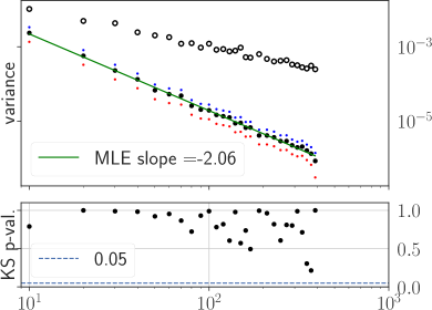
(a) $d=1$

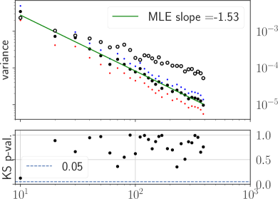
(b) $d=2$

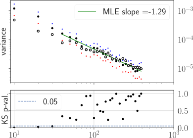
(c) $d=3$

Figure 5: Summary of the importance sampling results.

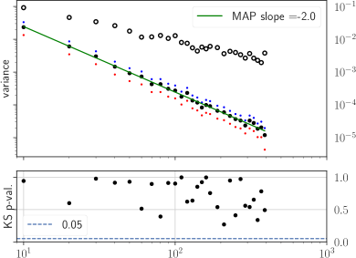
(a) $d=1$

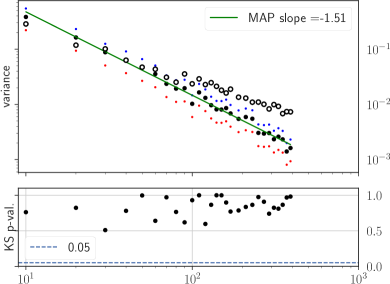
(b) $d=2$

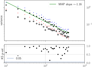
(c) $d=3$

Figure 6: Summary of the crude Monte Carlo results for a test function that violates the assumptions of Theorem 3.

References

• Ameur et al. [2011] Y. Ameur, H. Hedenmalm, and N. Makarov. Fluctuations of eigenvalues of random normal matrices. Duke Math. J., 159(1):31–81, 2011.
• Ameur et al. [2015] Y. Ameur, H. Hedenmalm, and N. Makarov. Random normal matrices and Ward identities. Ann. Probab., 43(3):1157–1201, 2015.
• Bach et al. [2012] F. Bach, S. Lacoste-Julien, and G. Obozinski. On the equivalence between herding and conditional gradient algorithms. In Proceedings of the International Conference on Machine Learning (ICML), 2012.
• Belloni and Chernozhukov [2009] A. Belloni and V. Chernozhukov. On the computational complexity of MCMC-based estimators in large samples. Annals of Statistics, 2009.
• Berman [2009a] R. J. Berman. Bergman kernels for weighted polynomials and weighted equilibrium measures of $\mathbb{C}^{n}$. Indiana Univ. Math. J., 58(4):1921–1946, 2009a.
• Berman [2009b] R. J. Berman. Bergman kernels and equilibrium measures for line bundles over projective manifolds. Amer. J. Math., 131(5):1485–1524, 2009b.
• Berman [2012] R. J. Berman. Sharp asymptotics for Toeplitz determinants and convergence towards the Gaussian free field on Riemann surfaces. Int. Math. Res. Not. IMRN, (22):5031–5062, 2012.
• Berman [2014] R. J. Berman. Determinantal point processes and fermions on complex manifolds: large deviations and bosonization. Comm. Math. Phys., 327(1):1–47, 2014.
• Berman [2018] R. J. Berman. Kähler-Einstein metrics, canonical random point processes and birational geometry. In Algebraic geometry: Salt Lake City 2015, Proc. Sympos. Pure Math. Amer. Math. Soc., Providence, RI, 2018.
• Bogaert [2014] I. Bogaert. Iteration-free computation of Gauss–Legendre quadrature nodes and weights. SIAM J. Sci. Comput., 36(3):A1008–1026, 2014.
• Brass and Petras [2011] H. Brass and K. Petras. Quadrature theory. Amer. Math. Soc., Providence, RI, 2011.
• Breuer and Duits [2016] J. Breuer and M. Duits. Universality of mesocopic fluctuation in orthogonal polynomial ensembles. Communications in Mathematical Physics, 2016.
• Breuer and Duits [2017] J. Breuer and M. Duits. Central limit theorems for biorthogonal ensembles and asymptotics of recurrence coefficients. J. Amer. Math. Soc., 30(1):27–66, 2017.
• Briol et al. [2015] F.-X. Briol, C. Oates, M. Girolami, and M. A. Osborne. Frank-Wolfe Bayesian quadrature: Probabilistic integration with theoretical guarantees. In Advances In Neural Information Processing Systems (NIPS), pages 1162–1170, 2015.
• Briol et al. [2019] F.-X. Briol, C. J. Oates, M. Girolami, M. A. Osborne, and D. Sejdinovic. Probabilistic integration: A role for statisticians in numerical analysis? Statistical Science, to appear, 2019.
• Chen et al. [2010] Y. Chen, M. Welling, and A. Smola. Super-samples from kernel herding. In Proceedings of the conference on Uncertainty in Artificial Intelligence (UAI), 2010.
• Daley and Vere-Jones [2003] D. J. Daley and D. Vere-Jones. An introduction to the theory of point processes. Springer, 2nd edition, 2003.
• Davis and Rabinowitz [1984] P. J. Davis and P. Rabinowitz. Methods of numerical integration. Academic Press, New York, 2nd edition, 1984.
• Delyon and Portier [2016] B. Delyon and F. Portier. Integral approximation by kernel smoothing. Bernoulli, 22(4), 2016.
• Diaconis and Evans [2001] P. Diaconis and S. N. Evans. Linear functionals of eigenvalues of random matrices. Trans. Amer. Math. Soc., 353(7):2615–2633, 2001.
• Dick and Pilichshammer [2010] J. Dick and F. Pilichshammer. Digital nets and sequences. Discrepancy theory and quasi-Monte Carlo Integration. Cambridge University Press, 2010.
• Dick et al. [2013] J. Dick, F. Y. Kuo, and I. H. Sloan. High-dimensional integration: the quasi-Monte Carlo way. Acta Numerica, 22:133–288, 2013.
• Douc et al. [2014] R. Douc, É. Moulines, and D. Stoffer. Nonlinear time series. Chapman-Hall, 2014.
• Fink et al. [2011] M. Fink, S. A. Niederer, E. M. Cherry, F. H. Fenton, J. T. Koivumäki, G. Seemann, R. Thul, H. Zhang, F. B. Sachse, E. J. Crampin, and N. P. Smith. Cardiac cell modelling: observations from the heart of the cardiac physiome project. Progress in biophysics and molecular biology, 104(1):2–21, 2011.
• Gauss [1815] C. F. Gauss. Methodus nova integralium valores per approximationem inveniendi. Heinrich Dietrich, Göttingen, 1815.
• Gautier et al. [2018] G. Gautier, R. Bardenet, and M. Valko. DPPy: Sampling determinantal point processes with Python. Arxiv preprint:1809.07258, 2018.
• Gautschi [2004] W. Gautschi. Orthogonal polynomials: computation and approximation. Oxford University Press, USA, 2004.
• Gautschi [2009] W. Gautschi. How sharp is Bernstein’s inequality for Jacobi polynomials. Electronic Transactions on Numerical Analysis, 36:1–8, 2009.
• Gautschi and Varga [1983] W. Gautschi and R. S. Varga. Error bounds for Gaussian quadrature of analytic functions. Siam J. Numer. Anal., 20(6):1170–1186, 1983.
• Glaser et al. [2007] A. Glaser, X. Liu, and V. Rokhlin. A fast algorithm for the calculation of the roots of special functions. SIAM Journal on Scientific Computing, 29(4):1420–1438, 2007.
• Glynn and Szechtman [2002] P. W. Glynn and R. Szechtman. Some new perspectives on the method of control variates. In Proceedings of Monte Carlo and Quasi-Monte Carlo Methods (MCQC 2000), pages 27–49. Springer, 2002.
• Golub and Van Loan [2012] G. H. Golub and C. F. Van Loan. Matrix computations. JHU Press, 2012.
• Hale and Townsend [2013] N. Hale and A. Townsend. Fast and accurate computation of Gauss-Legendre and Gauss-Jacobi quadrature nodes and weights. SIAM J. Sci. Comput., 35(2):A652–A674, 2013.
• Hardy [2015] A. Hardy. Average characteristic polynomials of determinantal point processes. Ann. Inst. H. Poincare Probab. Statist., 51(1):283–303, 2015.
• Hough et al. [2006] J. B. Hough, M. Krishnapur, Y. Peres, and B. Virág. Determinantal processes and independence. Probab. Surv., 3:206–229, 2006.
• Huszár and Duvenaud [2012] F. Huszár and D. Duvenaud. Optimally-weighted herding is Bayesian quadrature. In Uncertainty in Artificial Intelligence (UAI), 2012.
• Johansson [1997] K. Johansson. On random matrices from the compact classical groups. Ann. Math., 145(3):519–545, 1997.
• Johansson [1998] K. Johansson. On fluctuations of eigenvalues of random Hermitian matrices. Duke Math. J., 91(1):151–204, 1998.
• Johansson [2006] K. Johansson. Random matrices and determinantal processes, Mathematical Statistical Physics. Elsevier B.V. Amsterdam, 2006.
• Johansson and Lambert [2018] K. Johansson and G. Lambert. Gaussian and non-Gaussian fluctuations for mesoscopic linear statistics in determinantal processes. Ann. Probab., 46(3):1201–1278, 2018.
• Kallenberg [2006] O. Kallenberg. Foundations of modern probability. Springer Science & Business Media, 2006.
• Killip and Nenciu [2004] R. Killip and I. Nenciu. Matrix models for circular ensembles. International Mathematics Research Notices, 2004(50):2665–2701, 2004.
• König [2005] W. König. Orthogonal polynomial ensembles in probability theory. Probability Surveys, 2(385–447), 2005.
• Kriecherbauer and Shcherbina [2010] T. Kriecherbauer and M. Shcherbina. Fluctuations of eigenvalues of matrix models and their applications. Preprint arXiv:1003.6121, 2010.
• Kuijlaars et al. [2004] A. B. J. Kuijlaars, K. T.-R. McLaughlin, W. Van Assche, and M. Vanlessen. The Riemann-Hilbert approach to strong asymptotics for orthogonal polynomials on $[-1,1]$. Adv. Math., 188(2):337–398, 2004.
• Kulesza and Taskar [2012] A. Kulesza and B. Taskar. Determinantal point processes for machine learning. Foundations and Trends in Machine Learning, 2012.
• Lambert [2015] G. Lambert. CLT for biorthogonal ensembles and related combinatorial identities. Preprint arXiv:1511.06121, 2015.
• Lambert [2018] G. Lambert. Mesoscopic fluctuations for unitary invariant ensembles. Electron. J. Probab., 23:Paper No. 7, 33, 2018.
• Lavancier et al. [2015] F. Lavancier, J. M$\o$ller, and E. Rubak. Determinantal point process models and statistical inference. Journal of Royal Statistical Society: Series B (Statistical Methodology), 77:853–877, 2015.
• Liu and Lee [2017] Q. Liu and J. D. Lee. Black-box importance sampling. In Proceedings of the International Conference on Artificial Intelligence and Statistics (AISTATS), volume 54, pages 952–961, 2017.
• Lyons [2003] R. Lyons. Determinantal probability measures. Publ. Math. Inst. Hautes Etudes Sci., 98:167–212, 2003.
• Lyons and Peres [2016] R. Lyons and Y. Peres. Probabilities on trees and networks. Cambridge University Press, 2016.
• Macchi [1975] O. Macchi. The coincidence approach to stochastic point processes. Advances in Applied Probability, 7:83–122, 1975.
• Møller et al. [2015] J. Møller, M. Nielsen, E. Porcu, and E. Rubak. Determinantal point process models on the sphere. Research Report 13, Centre for Stochastic Geometry and Advanced Bioimaging. Submitted for journal publication., 2015.
• Oates and Girolami [2016] C. Oates and M. Girolami. Control functionals for quasi-Monte Carlo integration. In Proceeddings of the International conference on Artificial Intelligence and Statistics, 2016.
• Oates et al. [2017] C. J. Oates, M. Girolami, and N. Chopin. Control functionals for Monte Carlo integration. Journal of the Royal Statistical Society: Series B (Statistical Methodology), 79(3):695–718, 2017.
• O’Hagan [1991] A. O’Hagan. Bayes-Hermite quadrature. Journal of Statistical Planning and Inference, 29:245–260, 1991.
• Olver et al. [2015] S. Olver, R. R. Nadakuditi, and Trogdon T. Sampling unitary ensembles. Random Matrices Theory Appl., 4, 2015.
• Owen [1997] A. B. Owen. Scrambled net variance for integrals of smooth functions. The Annals of Statistics, 25(4):1541–1562, 1997.
• Owen [2008] A. B. Owen. Local antithetic sampling with scrambled nets. The Annals of Statistics, 36(5):2319–2343, 2008.
• Pastur [2006] L. Pastur. Limiting laws of linear eigenvalue statistics for Hermitian matrix models. J. Math. Phys., 47, 2006.
• Peet [2009] M. M. Peet. Exponentially stable nonlinear systems have polynomial Lyapunov functions on bounded regions. IEEE Trans. Automat. Control, 54(5):979–987, 2009.
• Popescu [2009] I. Popescu. General tridiagonal random matrix models, limiting distributions and fluctuations. Probabability Theory Related Fields, 144(1-2):179–220, 2009.
• Purves et al. [2013] D. Purves, J. P. W. Scharlemann, M. Harfoot, T. Newbold, D. P. Tittensor, J. Hutton, and S. Emmott. Ecosystems: Time to model all life on earth. Nature, 493:295–297, 2013.
• Rasmussen and Williams [2006] C. E. Rasmussen and C. K. I. Williams. Gaussian Processes for Machine Learning. MIT Press, 2006.
• Rider and Virág [2007] B. Rider and B. Virág. The noise in the circular law and the Gaussian free field. Int. Math. Res. Not., Art. ID rnm006(2):33 pp., 2007.
• Robert and Casella [2004] C. P. Robert and G. Casella. Monte Carlo Statistical Methods. Springer-Verlag, New York, 2004.
• Saff and Totik [1997] E. B. Saff and V. Totik. Logarithmic potentials with external fields. Number 316 in Grundlehren der Mathematischen Wissenschaften. Springer-Verlag, Berlin, 1997.
• Scardicchio et al. [2009] A. Scardicchio, C. E. Zachary, and S. Torquato. Statistical properties of determinantal point processes in high-dimensional euclidean spaces. Phys. Rev. E, (3) 79(4, 041108):19 pp., 2009.
• Schervish [2012] M. J. Schervish. Theory of statistics. Springer Science & Business Media, 2012.
• Shcherbina [2013] M. Shcherbina. Fluctuations of linear eigenvalue statistics of matrix models in the multicut regime. J. Stat. Phys., 151:1004–1034, 2013.
• Simon [2011] B. Simon. Szegő’s Theorem and its Descendants: Spectral Theory for $L^{2}$ Perturbations of Orthogonal Polynomials. M. B. Porter Lecture Series, Princeton Univ. Press, Princeton, NJ, 2011.
• Soshnikov [2000] A. Soshnikov. Determinantal random point fields. Russian Math. Surveys, 55:923–975, 2000.
• Soshnikov [2002] A. Soshnikov. Gaussian limit for determinantal random point fields. Ann. Probab., 30(1):171–187, 2002.
• Stahl and Totik [1992] H. Stahl and V. Totik. General orthogonal polynomials. Number 43 in Encyclopedia of Mathematics and its Applications. Cambridge University Press, Cambridge, 1992.
• Szegő [1974] G. Szegő. Orthogonal polynomials, volume Vol. XXIII. American Mathematical Society, Providence, R.I., 4th edition edition, 1974.
• Torquato et al. [2008] S. Torquato, A. Scardicchio, and C. E. Zachary. Point processes in arbitrary dimension from fermionic gases, random matrix theory, and number theory. J. Stat. Mech. Theory Exp., (11, P11019):39 pp., 2008.
• Trotta [2006] R. Trotta. Bayes in the sky: Bayesian inference and model selection in cosmology. Contemporary Physics, 2006.
• Xiang [2016] S. Xiang. An improved error bound on Gauss quadrature. Applied Mathematics Letters, 58:42–48, 2016.
• Xiang and Bornemann [2012] S. Xiang and F. Bornemann. On the convergence rates of Gauss and Clenshaw–Curtis quadrature for functions of limited regularity. SIAM J. Numer. Anal., 50(5):2581–2587, 2012.