MINIMAX RATES FOR ESTIMATING THE DIMENSION OF A MANIFOLD

Abstract

Many algorithms in machine learning and computational geometry require, as input, the intrinsic dimension of the manifold that supports the probability distribution of the data. This parameter is rarely known and therefore has to be estimated. We characterize the statistical difficulty of this problem by deriving upper and lower bounds on the minimax rate for estimating the dimension. First, we consider the problem of testing the hypothesis that the support of the data-generating probability distribution is a well-behaved manifold of intrinsic dimension $d_{1}$ versus the alternative that it is of dimension $d_{2}$, with $d_{1}<d_{2}$. With an i.i.d. sample of size $n$, we provide an upper bound on the probability of choosing the wrong dimension of $O\left(n^{-\left(d_{2}/d_{1}-1-\epsilon\right)n}\right)$, where $\epsilon$ is an arbitrarily small positive number. The proof is based on bounding the length of the traveling salesman path through the data points. We also demonstrate a lower bound of $\Omega\left(n^{-(2d_{2}-2d_{1}+\epsilon)n}\right)$, by applying Le Cam’s lemma with a specific set of $d_{1}$-dimensional probability distributions. We then extend these results to get minimax rates for estimating the dimension of well-behaved manifolds. We obtain an upper bound of order $O\left(n^{-(\frac{1}{m-1}-\epsilon)n}\right)$ and a lower bound of order $\Omega\left(n^{-(2+\epsilon)n}\right)$, where $m$ is the embedding dimension.

1 Introduction

Suppose that $X_{1},\ldots,X_{n}$ is an i.i.d. sample from a distribution $P$ whose support is an unknown, well-behaved, manifold $M$ of dimension $d$ in $\mathbb{R}^{m}$, where $1\leq d\leq m$. Manifold learning refers broadly to a suite of techniques from statistics and machine learning aimed at estimating $M$ or some of its features based on the data.

Manifold learning procedures are widely used in high dimensional data analysis, mainly to alleviate the curse of dimensionality. Such algorithms map the data to a new, lower dimensional coordinate system [Bellman, 1961, Lee and Verleysen, 2007a, Hastie et al., 2009], with little loss in accuracy. Manifold learning can greatly reduce the dimensionality of the data.

Most manifold learning techniques require, as input, the intrinsic dimension of the manifold. However, this quantity is almost never known in advance and therefore has to be estimated from the data.

Various intrinsic dimension estimators have been proposed and analyzed; [see, e.g., Lee and Verleysen, 2007b, Koltchinskii, 2000, Kégl, 2003, Levina et al., 2004, Hein and Audibert, 2005, Raginsky and Lazebnik, 2005, Little et al., 2009, 2011, Sricharan et al., 2010, Rozza et al., 2012, Camastra and Staiano, 2016]. However, characterizing the intrinsic statistical hardness of estimating the dimension remains an open problem.

The traditional way of measuring the difficulty of a statistical problem is to bound its minimax risk, which in the present setting is loosely described as the worst possible statistical performance of an optimal dimension estimator. Formally, given a class of probability distribution $\mathcal{P}$, the minimax risk $R_{n}=R_{n}(\mathcal{P})$ is defined as

$$R_{n}=\inf_{\widehat{d}_{n}}\sup_{P\in\mathcal{P}}\mathbb{E}_{P}\left[1(\widehat{d}_{n}\neq d(P))\right].$$ (1.1)

In Equation (1.1), $d(P)$ is the dimension of the support of $P$, $\mathbb{E}_{P}$ denotes the expectation with respect to the distribution $P$, $1(\cdot)$ is the indicator function, and the infimum is over all estimators (measurable functions of the data) $\widehat{d}_{n}=\widehat{d}_{n}(X_{1},\ldots,X_{n})$ of the dimension $d(P)$. The risk $\mathbb{E}_{P}[1(\widehat{d}_{n}\neq d(P))]$ of a dimension estimator $\widehat{d}_{n}$ is the probability that $\widehat{d}_{n}$ differs from the true dimension $d(P)$ of the support of the data generating distribution $P$. The minimax risk $R_{n}(\mathcal{P})$, which is a function of both the sample size $n$ and the class $\mathcal{P}$, quantifies the intrinsic hardness of the dimension estimation problem, in the sense that any dimension estimator cannot have a risk smaller than $R_{n}$ uniformly over every $P\in\mathcal{P}$.

The purpose of this paper is to obtain upper and lower bounds on the minimax risk $R_{n}$ in (1.1). We impose several regularity conditions on the set of manifolds supporting the distribution in the class $\mathcal{P}$, in order to make the problem analytically tractable and also to avoid pathological cases, such as space-filling manifolds. We first assume that the manifold supporting the data generating distribution $P$ has two possible dimensions, $d_{1}$ and $d_{2}$. This assumption is then relaxed to any dimension $d(P)$ between $1$ and the embedding dimension $m$. Our main result is the following theorem. See Section 2 for the definition of the class $\mathcal{P}$ of probability distributions supported on well-behaved manifolds in $\mathbb{R}^{m}$.

Theorem 1.

The minimax risk $R_{n}$ in (1.1) satisfies, $a_{n}\leq R_{n}\leq b_{n}$, where

$$a_{n} =(C_{K_{I}}^{(\ref*{prop:multidimension.lower})})^{n}\min\{\tau_{\ell}^{-4}n^{-2},1\}^{n},$$ (1.2)

$$b_{n} =(C_{K_{I},K_{p},K_{v},m}^{(\ref*{prop:multidimension.maximumrisk})})^{n}\max\left\{1,\tau_{g}^{-(m^{2}-m)n}\right\}n^{-\frac{n}{m-1}},$$ (1.3)

and the constants $\tau_{\ell}$, $\tau_{g}$, $C_{K_{I}}^{(\ref*{prop:multidimension.lower})}$ and $C_{K_{I},K_{p},K_{v},m}^{(\ref*{prop:multidimension.maximumrisk})}$ depend on $\mathcal{P}$ and are defined in Section 5.

We now make a few remarks about the previous theorem.

• Since the dimension $d(P)$ is a discrete quantity, the minimax rate $R_{n}$ in (1.1) is superexponential in sample size. This result seems at odds with the exponential rate obtained by [Koltchinskii, 2000, Proposition 2.1]. These different rates are due to different model assumptions. In [Koltchinskii, 2000] the data generating distribution is the convolution of a probability distribution supported on a manifold with a noise distribution supported on a set of full dimension $m$. In contrast, here we assume that the data are generated from a probability distribution supported on a manifold. Under our noiseless model, distributions supported on manifolds with different dimension are more easily distinguishable, hence the minimax rate $R_{n}$ converges to $0$ faster than under the model with noise assumed by [Koltchinskii, 2000].

• The key quantities that appear in the lower bound (1.2) and the upper bound (1.3) are the global reach $\tau_{g}$ and the local reach $\tau_{\ell}$ of the manifold, which are defined in Section 2. These reach parameters can be roughly thought as the inverse of the usual notion of curvature [see, e.g. Federer, 1959], and they affect the performance of any dimension estimator: a manifold with low reach may appear more space-filling than a manifold of the same dimension but with higher reach, thus making the task of resolving the dimension harder. Indeed, our analysis shows formally that the minimax risk $R_{n}$ in (1.1) decreases in the values of the reaches. Given their crucial role, we have attempted to make the dependence of the minimax risk $R_{n}$ on both $\tau_{g}$ and $\tau_{\ell}$ as explicit as possible.

• There is a gap between the lower bound (1.2) and the upper bound (1.3). Nonetheless, as far as we are aware, these are the most precise bounds on $R_{n}$ that are available.

This paper is organized as follows. In Section 2, we formulate and discuss regularity conditions on distributions and their supporting manifolds. In Section 3, we provide an upper bound on the minimax rate by considering the traveling salesman path through the points. In Section 4, we derive a lower bound on the minimax rate by applying Le Cam’s lemma with a specific set of $d_{1}$-dimensional and $d_{2}$-dimensional probability distributions. In Section 5, we extend our upper bound and lower bound for the case where the intrinsic dimension varies from $1$ to $m$.

2 Definitions and Regularity Conditions

In this section, we define the set $\mathcal{P}$ of probability distributions that we consider in bounding the minimax risk $R_{n}$ in (1.1). Such distributions are supported on manifolds whose dimension $d$ is between $1$ and $m$, where $m$ is the dimension of the embedding space. In particular, we require that the supporting manifolds have a uniform lower bound on their reach parameters $\tau_{g}$ and $\tau_{l}$. The resulting class of distributions is denoted by

$$\mathcal{P}=\bigcup_{d=1}^{m}\mathcal{P}_{\tau_{g},\tau_{\ell},K_{I},K_{v},K_{p}}^{d}.$$ (2.1)

In the rest of this section, we will make the definition $\mathcal{P}_{\tau_{g},\tau_{\ell},K_{I},K_{v},K_{p}}^{d}$ precise. Readers who are not interested in the details may skip the rest of the section. All the proofs for this section are in Section A.

2.1 Notation and Basic Definitions

For the reader’s convenience, we provide a list of the notation used throughout the paper in Table 1.

Notation	Definition
$1(\cdot)$	indicator function.
$d$, $d_{1}$, $d_{2}$	dimension of a manifold.
$\widehat{d}_{n}$	dimension estimator.
$dist_{A}(\cdot,\cdot)$	distance function on the set $A$.
$dist_{A,||\cdot||}(\cdot,\cdot)$	distance function on the set $A$ induced by the norm $||\cdot||$.
$\exp_{p}(\cdot)$	exponential map on point $p\in M$.
$\ell(\cdot,\cdot)$	loss function.
$n$	size of the sample.
$m$	dimension of the embedding space.
$p$, $q$	points on the manifold $M$.
$vol_{A}(\cdot)$	volume function of $A$.
$B_{A}(x,r)$	open ball with center $x$ and radius $r$, $\{y\in A:\,dist_{A}(y,x)<r\}$.
$C_{a_{1},\ldots,a_{k}}$	constant that depends only on $a_{1},\,\ldots,\,a_{k}$.
$I$	cube $[-K_{I},\,K_{I}]^{m}$.
$K_{I}$, $K_{v}$, $K_{p}$	fixed constants for regular conditions; see Definition 2.
$M$	manifold.
$P$	data generating probability distribution.
$R_{n}$	minimax risk $\underset{\widehat{d}_{n}}{\inf}\underset{P\in\mathcal{P}}{\sup}\mathbb{E}_{P}\left[1\left(\widehat{d}_{n}\neq d(P)\right)\right]$; see (1.1), (2.5), and (2.6).
$S_{n}$	permutation group on $\{1,\,\ldots,\,n\}$.
$T$	subset of $I^{n}\subset(\mathbb{R}^{d})^{n}$, used in Section 4.
$T_{p}M$	tangent space of a manifold $M$ at $p$.
$X_{1},\,\ldots,\,X_{n}$	sample points.
$\mathcal{M}$	set of manifolds; see Definition 2.
$\mathcal{P}$	set of distributions; see Definition 2.
$\gamma$	path on a manifold $M$.
$\pi_{A}(\cdot)$	projection function onto a closed set $A$.
$\sigma$	permutation.
$\tau(M)$	reach of a manifold $M$; see Definition 1 and Lemma 2.
$\tau_{g}$	lower bound for global reach; see Definition 2.
$\tau_{\ell}$	lower bound for local reach; see Definition 2.
$\omega_{d}$	volume of the unit ball in $\mathbb{R}^{d}$, $\frac{\pi^{\frac{d}{2}}}{\Gamma\left(\frac{d}{2}+1\right)}$.
$\Pi_{n_{1}:n_{2}}$	coordinate projection map: $\Pi_{n_{1}:n_{2}}(x_{1},\,\ldots,\,x_{d})=(x_{n_{1}},\,\ldots,\,x_{n_{d}})$.

Table 1: Table of notations and definitions.

We now briefly review some notations from differential geometry. For a more detailed treatment, we refer the reader to standard textbooks on this topic [see, e.g., Lee, 2000, 2003, Petersen, 2006, do Carmo, 1992]. A topological manifold of dimension $d$ is a topological space $M$ and a family of homeomorphisms $\varphi_{\alpha}:U_{\alpha}\subset\mathbb{R}^{d}\rightarrow V_{\alpha}\subset M$ from an open subset of $\mathbb{R}^{d}$ to an open subset of $M$ such that $\underset{\alpha}{\bigcup}\varphi_{\alpha}(U_{\alpha})=M$. A topological space $M$ is considered to be a $d$-dimensional manifold if there exists a family of homeomorphisms $\varphi_{\alpha}:U_{\alpha}\subset\mathbb{R}^{d}\rightarrow V_{\alpha}\subset M$ such that $(M,\{\varphi_{\alpha}\}_{\alpha})$ is a manifold. If $M$ is a $d$-dimensional manifold, such $d$ is unique and is called the dimension of a manifold. If, for any pair $\alpha$, $\beta$, with $\varphi_{\alpha}(U_{\alpha})\cap\varphi_{\beta}(U_{\beta})\neq\emptyset$, $\varphi_{\beta}^{-1}\circ\varphi_{\alpha}:U_{\alpha}\cap U_{\beta}\rightarrow U_{\alpha}\cap U_{\beta}$ is $C^{k}$, then $M$ is a $C^{k}$-manifold.

We assume that the topological manifold $M$ is embedded in $\mathbb{R}^{m}$, i.e. $M\subset\mathbb{R}^{m}$, and the metric is inherited from the metric of $\mathbb{R}^{m}$. For a topological manifold $M\subset\mathbb{R}^{m}$ and for any $p,\,q\in M$, a path joining $p$ to $q$ is a map $\gamma:[a,b]\rightarrow M$ for some $a,b\in\mathbb{R}$ such that $\gamma(a)=p$, $\gamma(b)=q$. The length of the curve $\gamma$ is defined as $Length(\gamma)=\int_{a}^{b}||\gamma^{\prime}(t)||_{2}dt$. A topological manifold $M$ is equipped with the distance $dist_{M}:M\times M\rightarrow\mathbb{R}$ as $dist_{M}(p,q)=\underset{\gamma:\text{ path joining }p\text{ and }q}{\inf}Length(\gamma)$. A path $\gamma:[a,b]\rightarrow M$ is a geodesic if for all $t,t^{\prime}\in[a,b]$, $dist_{M}(\gamma(t),\gamma(t^{\prime}))=|t-t^{\prime}|$.

Let $T_{p}M$ denote the tangent space to $M$ at $p$. Given $p\in M$, there exist a set $0\in\mathcal{E}\subset T_{p}(M)$ and a mapping $\exp_{p}:\mathcal{E}\subset T_{p}M\rightarrow M$ such that $t\rightarrow\exp_{p}(tv)$, $t\in(-1,1)$, is the unique geodesic of $M$ which, at $t=0$, passes through $p$ with velocity $v$, for all $v\in\mathcal{E}$. The map $\exp_{p}:\mathcal{E}\subset T_{p}M\rightarrow M$ is called the exponential map on $p$.

One of the key conditions that we impose in Section 2.3 is about the reach.

Definition 1.

For a compact $d$-dimensional topological manifold $M\subset\mathbb{R}^{m}$ (with boundary), the reach of $M$, $\tau(M)$, is defined as the largest value of $r>0$ such that each $x\in\mathbb{R}^{m}$ with $dist_{\mathbb{R}^{m}}(x,M)<r$ has a unique projection $\pi_{M}(x)$ on $M$, i.e.

$$\tau(M):=\sup\Bigl{\{}r:\, \forall x\in\mathbb{R}^{m}\text{ with }dist_{\mathbb{R}^{m}}(x,\,M)<r,$$

$$\exists!\pi_{M}(x)\in M\text{ s.t. }||x-\pi_{M}(x)||_{2}=\underset{y\in M}{\inf}||x-y||_{2}\Bigr{\}}.$$ (2.2)

See [Federer, 1959] for further details. The reach $\tau(M)$ can be also considered as one kind of curvature, and can be understood as an inverse of other usual curvatures. See Figure 2.11(a) for the illustration of Definition 1. There are several equivalent ways to define the reach $\tau(M)$ in (1) for the manifold $M$. The reach $\tau(M)$ is the maximum radius of a ball that can be rolled freely over the manifold $M$, as in Lemma 2. See Figure 2.11(b) for the illustration of Lemma 2.

Lemma 2.

For a manifold $M\subset\mathbb{R}^{m}$,

$$\tau(M)=\sup\bigl{\{}r:\, \forall x\in M,\,\forall y\in\mathbb{R}^{m}\text{ with }y-x\perp T_{x}M\text{ and }||y-x||_{2}=r,$$

$$B_{\mathbb{R}^{m}}(y,\,r)\cap M=\emptyset\bigr{\}}.$$ (2.3)

Proof of Lemma 2.

[See Federer, 1959, Theorem 4.18]. ∎

(a) reach $\tau(M)$ in Definition 1.

(b) reach $\tau(M)$ in Lemma 2.

Figure 2.1: For a manifold $M$, there are several equivalent definitions for reach $\tau(M)$ in Definition 1. 1(a) The reach $\tau(M)$ is the supremum value of $r$ such that for all $x\in\mathbb{R}^{m}$ with $dist_{\mathbb{R}^{m}}(x,M)<r$ has unique projection $\pi_{M}(x)$ to $M$, as in (1). 1(b) The reach $\tau(M)$ is the maximum radius of a ball that you can roll over the manifold $M$, as in (2).

2.2 Minimax Theory

The minimax rate is the risk of an estimator that performs best in the worst case, as a function of the sample size [see, e.g. Tsybakov, 2008]. Let $\mathcal{P}$ be a collection of probability distributions over the same sample space $\mathcal{X}$ and let $\theta:\mathcal{P}\rightarrow\Theta$ be a function over $\mathcal{P}$ taking values in some space $\Theta$, the parameter space. We can think of $\theta(P)$ as the feature of interest of the probability distribution $P$, such as its mean, or, as in our case, the dimension of its support. For the fixed sample size $n$, suppose $X=(X_{1},\ldots,X_{n})$ is an i.i.d. (independent and identically distributed) sample drawn from a fixed probability distribution $P\in\mathcal{P}$. Thus $X$ takes values in the $n$-fold product space $\mathcal{X}^{n}=\mathcal{X}\times\cdots\times\mathcal{X}$ and is distributed as $P^{(n)}$, the $n$-fold product measure. An estimator $\widehat{\theta}_{n}:\mathbb{R}^{n}\rightarrow\Theta$ is any measurable function that maps the observation $X$ into the parameter space $\Theta$. Let $\ell:\Theta\times\Theta\rightarrow\mathbb{R}$ be a loss function, a non-negative bounded function that measures how different two parameters are. Then for a fixed estimator $\widehat{\theta}_{n}$ and a fixed distribution $P$, the risk of $\widehat{\theta}_{n}$ is defined as

$$\mathbb{E}_{P^{(n)}}\left[\ell\left(\widehat{\theta}_{n}(X),\theta(P)\right)\right].$$

Then for a fixed estimator $\widehat{\theta}_{n}$, its maximum risk is the supremum of its risk over every distribution $P\in\mathcal{P}$, that is,

$$\underset{P\in\mathcal{P}}{\sup}\mathbb{E}_{P^{(n)}}\left[\ell\left(\widehat{\theta}_{n}(X),\theta(P)\right)\right].$$ (2.4)

The minimax risk associated with $\mathcal{P}$, $\theta$, $\ell$ and $n$ is the maximal risk of any estimator that performs the best under the worst possible choice of $P$. Formally, the minimax risk is

$$R_{n}=\inf_{\widehat{\theta}_{n}}\sup_{P\in\mathcal{P}}\mathbb{E}_{P^{(n)}}\left[\ell\left(\widehat{\theta}_{n}(X),\theta(P)\right)\right].$$ (2.5)

The minimax risk $R_{n}$ in (2.5) is often viewed as a function of the sample size $n$, in which case any positive sequence $\psi_{n}$ such that $\lim_{n\rightarrow\infty}R_{n}/\psi_{n}$ remains bounded away from $0$ and $\infty$ is called a minimax rate. Notice that minimax rates are unique up to constants and lower order terms.

To define a meaningful minimax risk, it is essential to have some constraint on the set of distributions $\mathcal{P}$ in (2.4) and (2.5). If $\mathcal{P}$ is too large, then the minimax rate $R_{n}$ in (2.5) will not converge to $0$ as $n$ goes to $\infty$: this means that the problem is statistically ill-posed. If $\mathcal{P}$ is too small, the minimax estimator depends too much on the specific distributions in $\mathcal{P}$ and is not a useful measure of a statistical difficulty.

Determining the value of the minimax risk $R_{n}$ in (2.5) for a given problem requires two separate calculations: an upper bound on $R_{n}$ and a lower bound. In order to derive an upper bound, one analyzes the asymptotic risk of a specific estimator $\widehat{\theta}_{n}$. Lower bounds are instead usually computed by measuring the difficulty of a multiple hypothesis testing problem that entails identifying finitely many distributions in $\mathcal{P}$ that are maximally difficult to discriminate [see, e.g. Tsybakov, 2008, Section 2.2].

For the dimension estimation problem, we obtain an upper bound on $R_{n}$ by analyzing the performance of an estimator based on the length of the traveling salesman problem, as described in Section 3. On the other hand, the calculation of the lower bound presents non-trivial technical difficulties, because probability distributions supported on manifolds of different dimensions are singular with respect to each other, and therefore trivially discriminable. In order to overcome such an issue, we resort to constructing mixtures of mutually singular distributions. We detail this construction in Section 4.

There is a gap between the lower and upper bounds we derive on the minimax risk, as it is often the case in such calculations. Nonetheless, the derivation of the bounds is of use in understanding the difficulty of the dimension estimation problem.

2.3 Regularity conditions on the Distributions and their Supporting Manifolds

In our analysis we require various regularity conditions on the class $\mathcal{P}$ of probability distributions appearing in the minimax risk (1.1). Most of these conditions are of a geometric nature and concern the properties of the manifolds supporting the probability distributions in $\mathcal{P}$. Altogether, our assumptions rule out manifolds that are so complicated to make the dimension estimation problem unsolvable and, therefore, guarantee that the minimax risk $R_{n}$ in (2.5) converges to $0$ as $n$ goes to $\infty$. Such regularity assumptions are quite mild, and in fact allow for virtually all types of manifolds usually encountered in manifold learning problems.

Our first assumption is that the probability distributions in $\mathcal{P}$ are supported over manifold contained inside a compact set, which, without loss of generality, we take to be the cube $I:=[-K_{I},K_{I}]^{m}$, for some $K_{I}>0$. See Figure 2.2.

Figure 2.2: A manifold $M$ is assumed to be contained inside the cube $I=[-K_{I},K_{I}]^{m}$, for some $K_{I}>0$. See Definition 2.

Second, to exclude manifolds that are arbitrarily complicated in the sense of having unbounded curvatures or of being nearly self intersecting, we assume that the reach is uniformly bounded from below. More precisely, we will constrain both the global reach and the local reach as follows. Fix $\tau_{g},\tau_{\ell}\in(0,\infty]$ with $\tau_{g}\leq\tau_{\ell}$. The global reach condition for a manifold $M$ is that the usual reach $\tau(M)$ in (1) is lower bounded by $\tau_{g}$ as in Figure 2.33(a), and the local reach condition is that $M$ can be covered by small patches whose reaches are lower bounded by $\tau_{\ell}$, as in Figure 2.33(b). (See Definition 2 below for more details.)

(a) global reach condition

(b) local reach condition

Figure 2.3: A manifold $M$ with 3(a) global reach at least $\tau_{g}$, or 3(b) local reach at least $\tau_{\ell}$. See Definition 2.

Third, we assume that the data are generated from a distribution $P$ supported on a manifold $M$ having a density with respect to the (restriction of the) Hausdorff measure on $M$ bounded from above by some positive constant $K_{p}$.

For manifolds without boundary, the above conditions suffice for our analysis. However, to deal with manifolds with boundary, we need further assumptions, namely local geodesic completeness and essential dimension. A manifold $M$ is said to be complete if any geodesic can be extended arbitrarily farther, i.e. for any geodesic path $\gamma:[a,b]\to M$, there exists a geodesic $\tilde{\gamma}:\mathbb{R}\to M$ that satisfies $\tilde{\gamma}|_{[a,b]}=\gamma$. [see, e.g., Lee, 2000, 2003, Petersen, 2006, do Carmo, 1992]. Accordingly, we define a manifold $M$ to be locally (geodesically) complete, if any two points inside a geodesic ball of small enough radius in the interior of $M$ can be joined by a geodesic whose image also lies on the interior of $M$.

Fifth, we assume the manifold $M$ is of essential dimension $d$, in volume sense. If we fix any point $p$ in the $d$-dimensional manifold $M$, then the volume of a ball of radius $r$ grows in order of $r^{d}$ when $r$ is small. By extending this, fix $K_{v}\in(0,2^{-m}]$, and we say that the manifold $M$ is of essential volume dimension $d$, if the volume of a geodesic ball of radius $r$ around any point in $M$ is lower bounded by $K_{v}r^{d}\omega_{d}$, for some positive constant $K_{v}$ and all $r$ small enough.

We are now ready to formally define the class $\mathcal{P}$ of probability distributions that we will consider in our analysis of the minimax problem (1.1).

Definition 2.

Fix $\tau_{g},\,\tau_{\ell}\in(0,\infty]$, $K_{I}\in[1,\infty)$, $K_{v}\in(0,2^{-m}]$, with $\tau_{g}\leq\tau_{\ell}$. Let $\mathcal{M}_{\tau_{g},\tau_{\ell},K_{I},K_{v}}^{d}$ be the set of compact $d$-dimensional manifolds $M$ such that:

• $M\subset I:=[-K_{I},K_{I}]^{m}\subset\mathbb{R}^{m}$;

• $M$ is of global reach at least $\tau_{g}$, i.e. $\tau(M)\geq\tau_{g}$, and $M$ is of local reach at least $\tau_{\ell}$, i.e. for all $p\in M$, there exists a neighborhood $U_{p}$ in $M$ such that $\tau(U_{p})\geq{\tau_{\ell}}$;

• $M$ is locally (geodesically) complete (with respect to $\tau_{g}$): for all $p\in{\rm int}(M)$ and for all $q_{1},q_{2}\in B_{M}(p,\,2\sqrt{3}\tau_{g})$, there exists a geodesic $\gamma$ joining $q_{1}$ and $q_{2}$ whose image lies on $intM$;

• $M$ is of essential volume dimension $d$ (with respect to $K_{v}$ and $\tau_{g}$): if for all $p\in M$ and for all $r\leq\sqrt{3}\tau_{g}$, $vol_{M}(B_{M}(p,r))\geq K_{v}r^{d}\omega_{d}$.

Let $\mathcal{P}=\mathcal{P}_{\tau_{g},\tau_{\ell},K_{I},K_{v},K_{p}}^{d}$ be the set of Borel probability distributions $P$ such that:

• $P$ is supported on a $d$-dimensional manifold $M\in\mathcal{M}_{\tau_{g},\tau_{\ell},K_{I},K_{v}}^{d}$;

• $P$ is absolutely continuous with respect to the restriction $vol_{M}$ of the $d$-dimensional Hausdorff measure on the supporting manifold $M$ and such that $\sup_{x\in M}\frac{dP}{dvol_{M}}(x)\leq K_{p}$.

For every $P\in\mathcal{P}_{\tau_{g},\tau_{\ell},K_{I},K_{v},K_{p}}^{d}$, denote the dimension of its distribution as $d(P)$.

Remark 1.

For manifolds without boundary, the local completeness condition and the essential volume dimension condition in Definition 2 always hold. The Hopf Rinow Theorem [see, e.g. Petersen, 2006, Theorem 16] implies that any compact closed manifold without boundary is geodesic complete, which implies it is locally complete in the sense of (3) in Definition 2. Also, [Niyogi et al., 2008, Lemma 5.3] implies that, for a $d$-dimensional manifold $M$ and all $0<r\leq 2\tau(M)$,

$$vol_{M}(B_{M}(p,r))\geq r^{d}\left(1-\left(\frac{r}{2\tau(M)}\right)^{2}\right)^{\frac{d}{2}}\omega_{d},$$

for all $p\in M$. Hence, when, for fixed $\tau_{g}>0$, a $d$-dimensional manifold $M$ (without boundary) satisfies $\tau(M)\geq\tau_{g}$, then for any $0<r\leq\sqrt{3}\tau_{g}$, $vol_{M}(B_{M}(p,r))\geq 2^{-d}r^{d}\omega_{d}$, so the essential volume dimension condition is satisfied.

Remark 2.

The notion of the local reach $\tau_{\ell}$ in Definition 2 is less standard than the global reach $\tau_{g}$, which is the usual definition of the reach in [see, e.g. Federer, 1959]. The local reach condition is only used in getting the lower bound of the minimax rate $R_{n}$ in Section 4, while the global reach condition is used in both Section 3 and Section 4. In fact, the reach of the manifold is determined either by a bottleneck structure or an area of high curvature, as in [Aamari et al., 2017, Theorem 3.4]. And the global reach condition is imposing regularities on both cases, while the local reach condition is imposing regularities only on the latter case, i.e. on the local curvature. Setting the local reach $\tau_{\ell}$ equal to the global reach $\tau_{g}$ reduces to the model that has conditions only on the usual reach.

The regularity conditions in Definition 2 imply further constraints on both the distributions in $\mathcal{P}$ and their supporting manifolds, in Lemma 3, 4, and 5. Such properties are exploited in Section 3 and 4. The proofs for Lemma 3, 4, and 5 are in Appendix A.

Lemma 3.

Fix $\tau_{g}\in(0,\infty]$, and let $M$ be a $d$-dimensional manifold with global reach $\geq\tau_{g}$. For $r\in(0,\tau_{g})$, let $M_{r}:=\{x\in\mathbb{R}^{m}:\ dist_{\mathbb{R}^{m},}(x,M)<r\}$ be an $r$-neighborhood of $M$ in $\mathbb{R}^{m}$. Then, the volume of $M$ is upper bounded as

$$vol_{M}(M)\leq\frac{m!}{d!}r^{d-m}vol_{\mathbb{R}^{m}}(M_{r}).$$

Further, fix $\tau_{\ell}\in(0,\infty]$, $K_{I}\in[1,\infty)$, $K_{v}\in(0,2^{-m}]$, with $\tau_{g}\leq\tau_{\ell}$, and suppose $M\in\mathcal{M}_{\tau_{g},\tau_{\ell},K_{I},K_{v}}^{d}$. Then the volume of $M$ is upper bounded as

$$vol_{M}(M)\leq C_{K_{I},m}^{(\ref*{lem:regular.bounded.volume})}\max\left\{1,\tau_{g}^{d-m}\right\},$$

where $C_{K_{I},m}^{(\ref*{lem:regular.bounded.volume})}$ is a constant depending only on $K_{I}$ and $m$.

Lemma 4.

Fix $\tau_{g},\,\tau_{\ell}\in(0,\infty]$, $K_{I}\in[1,\infty)$, $K_{v}\in(0,2^{-m}]$, with $\tau_{g}\leq\tau_{\ell}$. Let $M\in\mathcal{M}_{\tau_{g},\tau_{\ell},K_{I},K_{v}}^{d}$ and $r\in(0,2\sqrt{3}\tau_{g}]$. Then $M$ can be covered by $N$ radius $r$ balls $B_{M}(p_{1},r)$, $\ldots$, $B_{M}(p_{N},r)$, with

$$N\leq\left\lfloor\frac{2^{d}vol(M)}{K_{v}r^{d}\omega_{d}}\right\rfloor.$$

Lemma 5.

Fix $\tau_{g},\,\tau_{\ell}\in(0,\infty]$, $K_{I}\in[1,\infty)$, $K_{v}\in(0,2^{-m}]$, with $\tau_{g}\leq\tau_{\ell}$. Let $M\in\mathcal{M}_{\tau_{g},\tau_{\ell},K_{I},K_{v}}^{d}$ and let $\exp_{p_{k}}:\mathcal{E}_{k}\subset\mathbb{R}^{m}\rightarrow{\mathcal{M}}$ be an exponential map, where $\mathcal{E}_{k}$ is the domain of the exponential map $\exp_{p_{k}}$ and $T_{p_{k}}M$ is identified with $\mathbb{R}^{d}$. For all $v,w\in\mathcal{E}_{k}$, let $R_{k}:=\max\{||v||,||w||\}$. Then

$$\|\exp_{p_{k}}(v)-\exp_{p_{k}}(w)\|_{\mathbb{R}^{m}}\leq\frac{\sinh(\sqrt{2}R_{k}/\tau_{\ell})}{\sqrt{2}R_{k}/\tau_{\ell}}\|v-w\|_{\mathbb{R}^{d}}.$$

Under these regularity conditions, the minimax risk $R_{n}$ is defined as

$$R_{n}=\inf_{\widehat{d}_{n}}\sup_{P\in\mathcal{P}}\mathbb{E}_{P^{(n)}}\left[1\left(\widehat{d}_{n}(X)\neq d(P)\right)\right],$$ (2.6)

where in Section 3 and 4 we fix $d_{1},d_{2}\in\mathbb{N}$ with $1\leq d_{1}<d_{2}\leq m$ and define

$$\mathcal{P}=\mathcal{P}_{\tau_{g},\tau_{\ell},K_{I},K_{v},K_{p}}^{d_{1}}\bigcup\mathcal{P}_{\tau_{g},\tau_{\ell},K_{I},K_{v},K_{p}}^{d_{2}},$$ (2.7)

and in Section 5 we set instead

$$\mathcal{P}=\overset{m}{\underset{d=1}{\bigcup}}\mathcal{P}_{\tau_{g},\tau_{\ell},K_{I},K_{v},K_{p}}^{d}.$$ (2.8)

In (2.6), $\widehat{d}_{n}$ is any dimension estimator based on data $X=(X_{1},\ldots,X_{n})$, and the loss function $\ell(\cdot,\cdot)$ is $0-1$ loss, so for all $x,y\in\mathbb{R}$, $\ell(x,y)=1(x\neq y)$.

3 Upper Bound for Choosing Between Two Dimensions

In this section we provide an upper bound on the minimax rate $R_{n}$ in (2.6) when $d(P)$ can only take two known values. Fix $d_{1},\,d_{2}\in\mathbb{N}$ with $1\leq d_{1}<d_{2}\leq m$, and assume that the data are generated from a distribution $P\in\mathcal{P}$ such that either $d(P)=d_{1}$ or $d(P)=d_{2}$ as in (2.7). In this case, the minimax risk quantifies the statistical hardness of the hypothesis testing problem of deciding whether the data originate from a $d_{1}$ or $d_{2}$-dimensional distribution. In Section 5 we will relax this assumption and allow for the intrinsic dimension $d(P)$ to be any integer between $1$ and $m$ as in (2.8). All the proofs for this section are in Section B.

Our strategy to derive an upper bound on $R_{n}$ is to choose a particular estimator $\widehat{d}_{n}$ and then derive a uniform upper bound on its risk over the class $\mathcal{P}$ in (2.7), i.e. an upper bound for the quantity

$$\underset{P\in\mathcal{P}}{\sup}\mathbb{E}_{P^{(n)}}\left[1\left(\widehat{d}_{n}(X)\neq d(P)\right)\right],$$ (3.1)

where $P^{(n)}$ denotes the $n$-fold product of $P$. This will in turn yield an upper bound on the minimax risk $R_{n}$, since

$$R_{n}=\inf_{\widehat{d}_{n}}\sup_{P\in\mathcal{P}}\mathbb{E}_{P^{(n)}}\left[1\left(\widehat{d}_{n}(X)\neq d(P)\right)\right]\leq\sup_{P\in\mathcal{P}}\mathbb{E}_{P^{(n)}}\left[1\left(\widehat{d}_{n}(X)\neq d(P)\right)\right].$$ (3.2)

Naturally, choosing an appropriate estimator is critical to get a sharp bound. In Section 3.1, we define our dimension estimator $\widehat{d}_{n}$ and analyze its risk. From that analysis, we derive an upper bound on the minimax risk $R_{n}$ in (2.6) in Section 3.2.

3.1 Dimension Estimator and its Analysis

Our dimension estimator $\widehat{d}_{n}$ is based on the $d_{1}$-squared length of the TSP (Traveling Salesman Path) generated by the data. The $d_{1}$-squared length of the TSP generated by the data is the minimal $d_{1}$-squared length of all possible paths passing through each sample point $X_{i}$ once, which is

$$\underset{\sigma\in S_{n}}{\min}\left\{\overset{n-1}{\underset{i=1}{\sum}}\|X_{\sigma(i+1)}-X_{\sigma(i)}\|_{\mathbb{R}^{m}}^{d_{1}}\right\}.$$ (3.3)

Then, $\widehat{d}_{n}=d_{1}$ if and only if the $d_{1}$-squared length of the TSP is below a certain threshold; that is

$$\widehat{d}_{n}(X):=\begin{cases}d_{1},&if\ \underset{\sigma\in S_{n}}{\min}\left\{\overset{n-1}{\underset{i=1}{\sum}}\|X_{\sigma(i+1)}-X_{\sigma(i)}\|_{\mathbb{R}^{m}}^{d_{1}}\right\}\leq C_{K_{I},K_{v},m}^{(\ref*{lem:upper.lowerdim})}\max\left\{1,\tau_{g}^{d_{1}-m}\right\},\\ d_{2},&\text{otherwise.}\end{cases}$$ (3.4)

where $C_{K_{I},K_{v},m}^{(\ref*{lem:upper.lowerdim})}$ is a constant to be defined later.

We begin our analysis of the estimator $\widehat{d}_{n}$ with Lemma 6, which shows that $\widehat{d}_{n}$ makes an error with probability of order $O\left(n^{-\left(\frac{d_{2}}{d_{1}}-1\right)n}\right)$ if the correct dimension is $d_{2}$. Specifically, we demonstrate that, for any positive value $L$, the $d_{1}$-squared length of a piecewise linear path from $X_{1}$ to $X_{n}$, $\overset{n-1}{\underset{i=1}{\sum}}\|X_{i+1}-X_{i}\|_{\mathbb{R}^{m}}^{d_{1}}$, is upper bounded by $L$ with a very small probability of order $O\left(n^{-\left(\frac{d_{2}}{d_{1}}-1\right)n}\right)$, as in (3.5). Hence the $d_{1}$-squared length of the path is not likely to be bounded by any such threshold $L$.

Lemma 6.

Fix $\tau_{g},\,\tau_{\ell}\in(0,\infty]$, $K_{I}\in[1,\infty)$, $K_{v}\in(0,2^{-m}]$, $K_{p}\in[(2K_{I})^{m},\infty)$, $d_{1},\,d_{2}\in\mathbb{N}$, with $\tau_{g}\leq\tau_{\ell}$ and $1\leq d_{1}<d_{2}\leq m$. Let $X_{1},\ldots,X_{n}\sim P\in\mathcal{P}_{\tau_{g},\tau_{\ell},K_{I},K_{v},K_{p}}^{d_{2}}$. Then for all $L>0$,

$$P^{(n)}\left[\overset{n-1}{\underset{i=1}{\sum}}\|X_{i+1}-X_{i}\|_{\mathbb{R}^{m}}^{d_{1}}\leq L\right]\leq\frac{\left(C_{K_{I},K_{p},m}^{(\ref*{lem:upper.higherdim})}\right)^{n-1}L^{\frac{d_{2}}{d_{1}}(n-1)}\max\left\{1,\tau_{g}^{(d_{2}-m)(n-1)}\right\}}{(n-1)^{\left(\frac{d_{2}}{d_{1}}-1\right)(n-1)}(n-1)!},$$ (3.5)

where $C_{K_{I},K_{p},m}^{(\ref*{lem:upper.higherdim})}$ is a constant depending only on $K_{I}$, $K_{p}$, and $m$.

Proof of Lemma 6.

in Appendix B. ∎

Next, Lemma 7 shows that the estimator $\widehat{d}_{n}$ in (3.4) is always correct when the intrinsic dimension is $d_{1}$, as in (3.6). Specifically, the $d_{1}$-squared length of the TSP path in (3.3) is bounded by some positive threshold $C_{K_{I},K_{v},m}^{(\ref*{lem:upper.lowerdim})}\max\left\{1,\tau_{g}^{d_{1}-m}\right\}$. We take note that, when $d_{1}=1$, Lemma 7 is straightforward: the length of the TSP path in (3.3) is upper bounded by the length of curve $vol_{M}(M)$, as in Figure 3.1. This fact, combined with Lemma 3, which shows that $vol_{M}(M)\leq C_{K_{I},m}^{(\ref*{lem:regular.bounded.volume})}\max\left\{1,\tau_{g}^{1-m}\right\}$, yields the result. In particular, the constant $C_{K_{I},K_{v},m}^{(\ref*{lem:upper.lowerdim})}$ can be set as $C_{K_{I},K_{v},m}^{(\ref*{lem:upper.lowerdim})}=C_{K_{I},m}^{(\ref*{lem:regular.bounded.volume})}$.

Figure 3.1: When the manifold is a curve, the length of the TSP path $\underset{\sigma\in S_{n}}{\min}\left\{\overset{n-1}{\underset{i=1}{\sum}}\|X_{\sigma(i+1)}-X_{\sigma(i)}\|_{\mathbb{R}^{m}}\right\}$ in (3.3) is upper bounded by the length of the curve $vol_{M}(M)$.

When $d_{1}>1$, Lemma 7 is proved using Lemma 3, 4 and 5, along with the Hölder continuity of a $d_{1}$-dimensional space-filling curve [Steele, 1997, Buchin, 2008].

Lemma 7.

Fix $\tau_{g},\,\tau_{\ell}\in(0,\infty]$, $K_{I}\in[1,\infty)$, $K_{v}\in(0,2^{-m}]$, $d_{1}\in\mathbb{N}$, with $\tau_{g}\leq\tau_{\ell}$. Let $M\in\mathcal{M}_{\tau_{g},\tau_{\ell},K_{p},K_{v}}^{d_{1}}$ and $X_{1},\ldots,X_{n}\in M$. Then

$$\underset{\sigma\in S_{n}}{\min}\overset{n-1}{\underset{i=1}{\sum}}\|X_{\sigma(i+1)}-X_{\sigma(i)}\|_{\mathbb{R}^{m}}^{d_{1}}\leq C_{K_{I},K_{v},m}^{(\ref*{lem:upper.lowerdim})}\max\left\{1,\tau_{g}^{d_{1}-m}\right\},$$ (3.6)

where $C_{K_{I},K_{v},m}^{(\ref*{lem:upper.lowerdim})}$ is a constant depending only on $K_{I}$, $K_{v}$, and $m$.

Proof of Lemma 7.

in Appendix B. ∎

Proposition 8 below is the main result of this subsection and follows directly from Lemma 6 and Lemma 7 above. Indeed, when the intrinsic dimension is $d_{2}$, the risk of our estimator $\widehat{d}_{n}$, is of order $O\left(n^{-\left(\frac{d_{2}}{d_{1}}-1\right)n}\right)$ by Lemma 6 and the union bound. On the other hand, when the intrinsic dimension is $d_{1}$, the risk of our estimator $\widehat{d}_{n}$ is $0$, because of Lemma 7.

Proposition 8.

Fix $\tau_{g},\,\tau_{\ell}\in(0,\infty]$, $K_{I}\in[1,\infty)$, $K_{v}\in(0,2^{-m}]$, $K_{p}\in[(2K_{I})^{m},\infty)$, $d_{1},\,d_{2}\in\mathbb{N}$, with $\tau_{g}\leq\tau_{\ell}$ and $1\leq d_{1}<d_{2}\leq m$. Let $\widehat{d}_{n}$ be in (3.4). Then either for $d=d_{1}$ or $d=d_{2}$,

$$\underset{P\in\mathcal{P}_{\tau_{g},\tau_{\ell},K_{I},K_{v},K_{p}}^{d}}{\sup}\mathbb{E}_{P^{(n)}}\left[\ell\left(\widehat{d}_{n},d(P)\right)\right]$$

$$\leq 1(d=d_{2})\left(C_{K_{I},K_{p},K_{v},m}^{(\ref*{prop:upper.maximumrisk})}\right)^{n}\max\left\{1,\tau_{g}^{-\left(\frac{d_{2}}{d_{1}}m+m-2d_{2}\right)n}\right\}n^{-\left(\frac{d_{2}}{d_{1}}-1\right)n},$$

where $C_{K_{I},K_{p},K_{v},m}^{(\ref*{prop:upper.maximumrisk})}\in(0,\infty)$ is a constant depending only on $K_{I}$, $K_{p}$, $K_{v}$, and $m$.

Proof of Proposition 8.

in Appendix B. ∎

As described so far, the convergence analysis of our dimension estimator is probable. This is enough for our purpose, which is to quantify the statistical difficulties, in particular the minimax rate, of the dimension estimation problem. However, our $\widehat{d}_{n}$ in (3.4) is not completely data-driven but depends on the model parameters $\tau_{g}$, $K_{I}$, and $K_{v}$. Hence the model on which our convergence analysis is valid depends on the model parameters. When it comes to applying our dimension estimator $\widehat{d}_{n}$ to real data, we need to estimate the constant $C_{K_{I},K_{v},m}^{(\ref*{lem:upper.lowerdim})}$. Proofs of Lemma 6 and 7 suggest that overestimating $C_{K_{I},K_{v},m}^{(\ref*{lem:upper.lowerdim})}$ by some constant factor doesn’t deteriorate the convergence rate, so the constants $C_{K_{I},K_{v},m}^{(\ref*{lem:upper.lowerdim})}$ and $\tau_{g}$ can be replaced by any consistent estimators. Still, we have the difficulty of tuning the constant $C_{K_{I},K_{v},m}^{(\ref*{lem:upper.lowerdim})}$ and $\tau_{g}$. Also, the constant $C_{K_{I},K_{v},m}^{(\ref*{lem:upper.lowerdim})}$ is tuned to work for the worst case, so the practical performance of our dimension estimator is questionable.

3.2 Minimax Upper Bound

As noted at the beginning of Section 3, the maximum risk of our estimator $\widehat{d}_{n}$ in (3.1) serves as an upper bound on the minimax risk $R_{n}$ in (2.6). Since we assume that the intrinsic dimension is either $d_{1}$ or $d_{2}$, Proposition 8 yields that the maximum risk of our estimator $\widehat{d}_{n}$ is of order $O\left(n^{-\left(\frac{d_{2}}{d_{1}}-1\right)n}\right)$. This also serves as an upper bound of the minimax risk $R_{n}$, as in Proposition 9.

Proposition 9.

Fix $\tau_{g},\,\tau_{\ell}\in(0,\infty]$, $K_{I}\in[1,\infty)$, $K_{v}\in(0,2^{-m}]$, $K_{p}\in[(2K_{I})^{m},\infty)$, $d_{1},\,d_{2}\in\mathbb{N}$, with $\tau_{g}\leq\tau_{\ell}$ and $1\leq d_{1}<d_{2}\leq m$. Then

$$\underset{\widehat{d}_{n}}{\inf}\underset{P\in\mathcal{P}_{1}\cup\mathcal{P}_{2}}{\sup}\mathbb{E}_{P^{(n)}}\left[\ell\left(\widehat{d}_{n},d(P)\right)\right]$$

$$\leq\left(C_{K_{I},K_{p},K_{v},m}^{(\ref*{prop:upper.maximumrisk})}\right)^{n}\max\left\{1,\tau_{g}^{-\left(\frac{d_{2}}{d_{1}}m+m-2d_{2}\right)n}\right\}n^{-\left(\frac{d_{2}}{d_{1}}-1\right)n},$$

where $C_{K_{I},K_{p},K_{v},m}^{(\ref*{prop:upper.maximumrisk})}$ is from Proposition 8 and

$$\mathcal{P}_{1}=\mathcal{P}_{\tau_{g},\tau_{\ell},K_{I},K_{v},K_{p}}^{d_{1}},\ \ \ \mathcal{P}_{2}=\mathcal{P}_{\tau_{g},\tau_{\ell},K_{I},K_{v},K_{p}}^{d_{2}}.$$

Proof of Proposition 9.

in Appendix B. ∎

4 Lower Bound for Choosing Between Two Dimensions

The goal of this section is to derive a lower bound for the minimax rate $R_{n}$. As in Section 3, we fix $d_{1},\,d_{2}\in\mathbb{N}$ with $1\leq d_{1}<d_{2}\leq m$, and assume that the intrinsic dimension of data is either $d_{1}$ or $d_{2}$ as in (2.7). This assumption is relaxed in Section 5. All the proofs for this section are in Section C.

Our strategy is to find a subset $T\subset I^{n}\subset(\mathbb{R}^{d})^{n}$ and two sets of distributions $\mathcal{P}_{1}^{d_{1}}$ and $\mathcal{P}_{2}^{d_{2}}$ with dimensions $d_{1}$ and $d_{2}$, such that $\mathcal{P}_{1}^{d_{1}}$ and $\mathcal{P}_{2}^{d_{2}}$ satisfy the regularity conditions in Definition 2, and whenever the sample $X=(X_{1},\ldots,X_{n})$ lies on $T$, one cannot easily distinguish whether the underlying distribution is from $\mathcal{P}_{1}^{d_{1}}$ or $\mathcal{P}_{2}^{d_{2}}$.

After constructing $T$, $\mathcal{P}_{1}^{d_{1}}$ and $\mathcal{P}_{2}^{d_{2}}$, we derive the lower bound using the following result, known as Le Cam’s lemma.

Lemma 10.

(Le Cam’s Lemma) Let $\mathcal{P}$ be a set of probability measures on $(\Omega,\mathcal{F})$, and $\mathcal{P}_{1},\mathcal{P}_{2}\subset\mathcal{P}$ be such that for all $P\in\mathcal{P}_{i}$, $\theta(P)=\theta_{i}$ for $i=1,2$. For any $Q_{i}\in co(\mathcal{P}_{i})$, where $co(\mathcal{P}_{i})$ is the convex hull of $\mathcal{P}_{i}$, let $q_{i}$ be the density of $Q_{i}$ with respect to a measure $\nu$. Then

$$\underset{\widehat{\theta}}{\inf}\underset{P\in\mathcal{P}}{\sup}\mathbb{E}_{P}[\ell(\widehat{\theta},\theta(P))]\geq\frac{\ell(\theta_{1},\theta_{2})}{2}\int[q_{1}(x)\wedge q_{2}(x)]d\nu(x).$$ (4.1)

Proof of Lemma 10.

[See Yu, 1997, Chapter 29.2, Lemma 1]. ∎

In above Le Cam’s lemma, considering the convex hull of distributions $co(\mathcal{P}_{i})$ is critical for getting the nontrivial lower bound. Suppose we are using the basic version of Le Cam’s lemma where the convex hull is not considered, i.e. $Q_{i}\in\mathcal{P}_{i}$. Then for two distributions $Q_{1}$ and $Q_{2}$ respectively from our $d_{1}$ and $d_{2}$ dimensional model $\mathcal{P}^{d_{1}}_{\tau_{g},\tau_{l},K_{I},K_{v},K_{p}}$ and $\mathcal{P}^{d_{2}}_{\tau_{g},\tau_{l},K_{I},K_{v},K_{p}}$, $Q_{1}$ and $Q_{2}$ are singular to each other; i.e. $q_{1}(x)\wedge q_{2}(x)=0$ for all $x$. Hence no matter which subset $\mathcal{P}_{1}$ and $\mathcal{P}_{2}$ we choose with $d(\mathcal{P}_{1})=d_{1}$ and $d(\mathcal{P}_{2})=d_{2}$, the lower bound in (4.1) will be always $0$. This trivial bound can be improved by considering the convex hull of distributions $co(\mathcal{P}_{i})$ in Le Cam’s lemma.

Our construction for $T$, $\mathcal{P}_{1}^{d_{1}}$, and $\mathcal{P}_{2}^{d_{2}}$ is based on mimicking a space-filling curve. Intuitively, this gives the lower bound since it is difficult to differentiate a space-filling curve and a higher dimensional cube. In detail, we set

$$\mathcal{P}_{1}^{d_{1}}=\{$$ distributions supported on

$$\text{a space-filling-curve like }d_{1}\text{-dimensional manifold}\},$$ (4.2)

and

$$\mathcal{P}_{2}^{d_{2}}=\{\text{uniform distributions on }[-K_{I},\,K_{I}]^{d_{2}}\}.$$ (4.3)

To apply Le Cam’s lemma, we construct a set $T\subset I^{n}$ so that, whenever $X=(X_{1},\ldots,X_{n})\in{T}$, we cannot distinguish whether $X$ is from $\mathcal{P}_{1}^{d_{1}}$ in (4) or $\mathcal{P}_{1}^{d_{2}}$ in (4.3). Then, for an appropriately chosen distribution $Q_{1}$ in the convex hull of $\mathcal{P}_{1}^{d_{1}}$ with density $q_{1}$ with respect to Lebesgue measure $\lambda$ on the cube $[-K_{I},K_{I}]^{d_{2}}$, and a density $q_{2}$ from the class $\mathcal{P}_{2}^{d_{2}}$, $\int_{T}[q_{1}(x)\wedge q_{2}(x)]d\lambda(x)$ is a lower bound on the minimax rate $R_{n}$ in (2.6). Indeed, from Le Cam’s Lemma 10, we have that

$$\underset{\widehat{\theta}}{\inf}\underset{P\in\mathcal{P}}{\sup}\mathbb{E}_{P}[\ell(\widehat{\theta},\theta(P))] \geq\frac{1}{2}\int[q_{1}(x)\wedge q_{2}(x)]d\lambda(x)$$

$$\geq\frac{1}{2}\int_{T}[q_{1}(x)\wedge q_{2}(x)]d\lambda(x).$$ (4.4)

For constructing the class $\mathcal{P}_{1}^{d_{1}}$ in (4), it will be sufficient to consider the case $d_{1}=1$. In fact, Lemma 11 states that the regularity conditions in Definition 2 are still preserved when the manifold $M$ is a Cartesian product with a cube $[-K_{I},\,K_{I}]^{\Delta d}$, as in Figure 4.1. Hence for constructing a $d$-dimensional “space-filling" manifold, we first construct a $1$-dimensional space-filling curve satisfying the required regularity conditions, and then we form a Cartesian product with a cube of dimension $d-1$, which becomes a $d$-dimensional manifold satisfying the same regularity conditions by Lemma 11.

Figure 4.1: The regularity conditions in Definition 2 are still preserved under the Cartesian product with a cube $[-K_{I},\,K_{I}]^{\Delta d}$. Detailed explanations are in Figure C.1.

Lemma 11.

Fix $\tau_{g},\,\tau_{\ell}\in(0,\infty]$, $K_{I}\in[1,\infty)$, $K_{v}\in(0,2^{-m}]$, $d,\,\Delta d\in\mathbb{N}$, with $\tau_{g}\leq\tau_{\ell}$ and $1\leq d+\Delta d\leq m$. Let $M\in\mathcal{M}_{\tau_{g},\tau_{\ell},K_{I},K_{v}}^{d}$ be a $d$-dimensional manifold of global reach $\geq\tau_{g}$, local reach $\geq\tau_{\ell}$, which is embedded in $\mathbb{R}^{m-\Delta d}$. Then

$$M\times[-K_{I},K_{I}]^{\Delta d}\in\mathcal{M}_{\tau_{g},\tau_{\ell},K_{I},K_{v}}^{d+\Delta d},$$

which is embedded in $\mathbb{R}^{m}$.

Proof of Lemma 11.

in Appendix C. ∎

The precise construction of $\mathcal{P}_{1}^{d_{1}}$ in (4) and $T$ is detailed in Lemma 12. As in Figure 4.2, we construct $T_{i}$’s that are cylinder sets aligned as a zigzag in $[-K_{I},K_{I}]^{d_{2}}$, and then $T$ is constructed as $T=S_{n}\overset{n}{\underset{i=1}{\prod}}T_{i}$, where the permutation group $S_{n}$ acts on $\overset{n}{\underset{i=1}{\prod}}T_{i}$ as a coordinate change. Then, we show below that, for any $x\in\prod T_{i}$, there exists a manifold $M\in\mathcal{M}_{\tau_{g},\tau_{\ell},K_{I},K_{v}}^{d_{1}}$ that passes through $x_{1},\ldots,x_{n}$. The class $\mathcal{P}_{1}^{d_{1}}$ in (4) is finally defined as the set of distributions that are supported on such a manifold.

(a) alignment of $T_{i}$

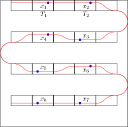
(b) manifold passing through $x_{i}$’s

Figure 4.2: This figure illustrates the case where $d_{1}=1$ and $d_{2}=2$. 2(a) shows how $T_{i}$’s are aligned in a zigzag. 2(b) shows for given $x_{1}\in T_{1},\ldots,x_{n}\in T_{n}$(represented as blue points), how a manifold with regularity conditions(represented as a red curve) passes through $x_{1},\ldots,x_{n}$. Detailed constructions in Figure 2(b).

Lemma 12.

Fix $\tau_{\ell}\in(0,\infty]$, $K_{I}\in[1,\infty)$, $d_{1},\,d_{2}\in\mathbb{N}$, with $1\leq d_{1}\leq d_{2}$, and suppose $\tau_{\ell}<K_{I}$. Then there exist $T_{1},\ldots,T_{n}\subset[-K_{I},K_{I}]^{d_{2}}$ such that:

(1) The $T_{i}$’s are distinct.

(2) For each $T_{i}$, there exists an isometry $\Phi_{i}$ such that

$$T_{i}=\Phi_{i}\left([-K_{I},K_{I}]^{d_{1}-1}\times[0,a]\times B_{\mathbb{R}^{d_{2}-d_{1}}}(0,w)\right),$$

where $c=\left\lceil\frac{K_{I}+\tau_{\ell}}{2\tau_{\ell}}\right\rceil$, $a=\frac{K_{I}-\tau_{\ell}}{\left(d_{2}-d_{1}+\frac{1}{2}\right)\left\lceil\frac{n}{c^{d_{2}-d_{1}}}\right\rceil}$, and $w=\min\left\{\tau_{\ell},\ \frac{(d_{2}-d_{1})^{2}(K_{I}-\tau_{\ell})^{2}}{2\tau_{\ell}\left(d_{2}-d_{1}+\frac{1}{2}\right)^{2}\left(\left\lceil\frac{n}{c^{d_{2}-d_{1}}}\right\rceil+1\right)^{2}}\right\}$.

(3)There exists $\mathscr{M}:\left(B_{\mathbb{R}^{d_{2}-d_{1}}}(0,w)\right)^{n}\rightarrow\mathcal{M}_{\tau_{g},\tau_{\ell},K_{I},K_{v}}^{d_{1}}$ one-to-one such that for each $y_{i}\in B_{\mathbb{R}^{d_{2}-d_{1}}}(0,w)$, $1\leq i\leq n$, $\mathscr{M}(y_{1},\ldots,y_{n})\cap T_{i}=\Phi_{i}([-K_{I},K_{I}]^{d_{1}-1}\times[0,a]\times\{y_{i}\})$. Hence for any $x_{1}\in T_{1},\ldots,x_{n}\in T_{n}$, $\mathscr{M}(\{\Pi_{(d_{1}+1):d_{2}}^{-1}\Phi_{i}^{-1}(x_{i})\}_{1\leq i\leq n})$ passes through $x_{1},\ldots,x_{n}$.

Proof of Lemma 12.

in Appendix C. ∎

Next we show that whenever $x=(x_{1},\ldots,x_{n})\in T$, it is difficult to tell whether the data originated from $P\in\mathcal{P}_{1}^{d_{1}}$ or $P\in\mathcal{P}_{2}^{d_{2}}$. Let $Q_{1}$ be in the convex hull of $\mathcal{P}_{1}^{d_{1}}$ and let $q_{2}$ be the density function of the uniform distribution on $[-K_{I},K_{I}]^{d_{2}}$, then from (4.4), we know that a lower bound is given by $\int_{T}[q_{1}(x)\wedge q_{2}(x)]d\lambda(x)$. Hence if we can choose $Q_{1}$ such that $q_{1}(x)\geq Cq_{2}(x)$ for every $x\in T$ with $C<1$, then $q_{1}(x)\wedge q_{2}(x)\geq Cq_{2}(x)$, so that $C\int_{T}q_{2}(x)$ can serve as a lower bound of the minimax rate. Such existence of $Q_{1}$ and the inequality $q_{1}(x)\geq Cq_{2}(x)$ is shown in Claim 13.

Claim 13.

Let $T=S_{n}\overset{n}{\underset{i=1}{\prod}}T_{i}$ where the $T_{i}$’s are from Lemma 12. Let $Q_{2}$ be the uniform distribution on $[-K_{I},K_{I}]^{d_{2}}$, and let $\mathcal{P}_{1}^{d_{1}}$ be as in (4). Then there exists $Q_{1}\in co(\mathcal{P}_{1}^{d_{1}})$ satisfying that for all $x\in intT$, there exists $r_{x}>0$ such that for all $r<r_{x}$,

$$Q_{1}\left(\overset{n}{\underset{i=1}{\prod}}B_{\|\cdot\|_{\mathbb{R}^{d_{2}},\infty}}(x_{i},r)\right)\geq 2^{-n}Q_{2}\left(\overset{n}{\underset{i=1}{\prod}}B_{\|\cdot\|_{\mathbb{R}^{d_{2}},\infty}}(x_{i},r)\right).$$

Proof of Claim 13.

in Appendix C. ∎

The following lower bound is then a consequence of Le Cam’s lemma, Lemma 12, and the previous claim.

Proposition 14.

Fix $\tau_{g},\,\tau_{\ell}\in(0,\infty]$, $K_{I}\in[1,\infty)$, $K_{v}\in(0,2^{-m}]$, $K_{p}\in[(2K_{I})^{m},\infty)$, $d_{1},\,d_{2}\in\mathbb{N}$, with $\tau_{g}\leq\tau_{\ell}$ and $1\leq d_{1}<d_{2}\leq m$, and suppose that $\tau_{\ell}<K_{I}$. Then

$$\underset{\widehat{d}_{n}}{\inf}\underset{P\in{\cal Q}}{\sup}\mathbb{E}_{P^{(n)}}[\ell(\widehat{d}_{n},d(P))]$$

$$\geq\left(C_{d_{1},d_{2},K_{I}}^{(\ref*{prop:lower.bound})}\right)^{n}\min\left\{\tau_{\ell}^{-2(d_{2}-d_{1}+1)}n^{-2},1\right\}^{(d_{2}-d_{1})n},$$

where $C_{d_{1},d_{2},K_{I}}^{(\ref*{prop:lower.bound})}\in(0,\infty)$ is a constant depending only on $d_{1}$, $d_{2}$, and $K_{I}$ and

$${\cal Q}=\mathcal{P}_{\tau_{g},\tau_{\ell},K_{I},K_{v},K_{p}}^{d_{1}}\bigcup\mathcal{P}_{\tau_{g},\tau_{\ell},K_{I},K_{v},K_{p}}^{d_{2}}.$$

Proof of Proposition 14.

in Appendix C. ∎

5 Upper Bound and Lower Bound for the General Case

Now we generalize our results to allow the intrinsic dimension $d$ to be any integer between 1 and $m$. Thus the model is $\mathcal{P}=\overset{m}{\underset{d=1}{\bigcup}}\mathcal{P}_{\tau_{g},\tau_{\ell},K_{I},K_{v},K_{p}}^{d}$ as in (2.8). For the upper bound, we extend the dimension estimator $\widehat{d}_{n}$ in (3.4) and compute its maximum risk. And for the lower bound, we simply use the lower bound derived in Section 4 with $d_{1}=1$ and $d_{2}=2$. All the proofs for this section are in Section D.

For the model $\mathcal{P}$ in (2.8), our dimension estimator $\widehat{d}_{n}$ estimates the dimension as the smallest integer $1\leq d\leq m$ that the $d$-squared length of the TSP is below a certain threshold, i.e. (3.6) holds; that is,

$$\widehat{d}_{n}(X):=\min\Biggl{\{} d\in[1,m]:\$$

$$\underset{\sigma\in S_{n}}{\min}\biggl{\{}\overset{n-1}{\underset{i=1}{\sum}}\|X_{\sigma(i+1)}-X_{\sigma(i)}\|_{\mathbb{R}^{m}}^{d}\biggr{\}}\leq C_{K_{I},K_{v},m}^{(\ref*{lem:upper.lowerdim})}\max\left\{1,\tau_{g}^{d-m}\right\}\Biggr{\}}.$$ (5.1)

As a generalized result of Proposition 8, Proposition 15 gives an upper bound for the risk of our estimator $\widehat{d}_{n}$ in (5). When the intrinsic dimension is $d$, our estimator $\widehat{d}_{n}$ makes an error with probability of order $O\left(n^{-\frac{1}{d-1}n}\right)$.

Proposition 15.

Fix $\tau_{g},\,\tau_{\ell}\in(0,\infty]$, $K_{I}\in[1,\infty)$, $K_{v}\in(0,2^{-m}]$, $K_{p}\in[(2K_{I})^{m},\infty)$, with $\tau_{g}\leq\tau_{\ell}$. Let $\widehat{d}_{n}$ be in (5). Then:

$$\underset{P\in\mathcal{P}_{\tau_{g},\tau_{\ell},K_{I},K_{v},K_{p}}^{d}}{\sup}\mathbb{E}_{P^{(n)}}\left[\ell\left(\widehat{d}_{n},d(P)\right)\right]$$

$$\leq 1(d>1)\left(C_{K_{I},K_{p},K_{v},m}^{(\ref*{prop:multidimension.maximumrisk})}\right)^{n}\max\left\{1,\tau_{g}^{-(dm+m-2d)n}\right\}n^{-\frac{1}{d-1}n},$$

where $C_{K_{I},K_{p},K_{v},m}^{(\ref*{prop:multidimension.maximumrisk})}\in(0,\infty)$ is a constant depending only on $K_{I}$, $K_{p}$, $K_{v}$, and $m$.

Proof of Proposition 15.

in Appendix D. ∎

Then similarly to Section 3.2, the maximum risk of our estimator $\widehat{d}_{n}$ in (5) serves as an upper bound on the minimax risk $R_{n}$ in (2.6). The maximum of the upper bound in Proposition 15 over $d$ ranging from $1$ to $m$ should serve as the upper bound for the maximum risk, hence we get the upper bound of the minimax risk $R_{n}$ in Proposition 16 as a generalized result of Proposition 9.

Proposition 16.

Fix $\tau_{g},\,\tau_{\ell}\in(0,\infty]$, $K_{I}\in[1,\infty)$, $K_{v}\in(0,2^{-m}]$, $K_{p}\in[(2K_{I})^{m},\infty)$, with $\tau_{g}\leq\tau_{\ell}$. Then:

$$\underset{\widehat{d}_{n}}{\inf}\underset{P\in\mathcal{P}}{\sup}\mathbb{E}_{P^{(n)}}\left[\ell\left(\widehat{d}_{n},d(P)\right)\right]\leq\left(C_{K_{I},K_{p},K_{v},m}^{(\ref*{prop:multidimension.maximumrisk})}\right)^{n}\max\left\{1,\tau_{g}^{-(m^{2}-m)n}\right\}n^{-\frac{1}{m-1}n},$$

where $C_{K_{I},K_{p},K_{v},m}^{(\ref*{prop:multidimension.maximumrisk})}$ is from Proposition 15.

Proof of Proposition 16.

in Appendix D. ∎

Proposition 17 provides a lower bound for the minimax rate $R_{n}$ in (2.6), in multi-dimensions. It can be viewed of a generalization for the binary dimension case in Proposition 14.

Proposition 17.

Fix $\tau_{g},\,\tau_{\ell}\in(0,\infty]$, $K_{I}\in[1,\infty)$, $K_{v}\in(0,2^{-m}]$, $K_{p}\in[(2K_{I})^{m},\infty)$, with $\tau_{g}\leq\tau_{\ell}$, and suppose that $\tau_{\ell}<K_{I}$. Then,

$$\underset{\widehat{d}_{n}}{\inf}\underset{P\in\mathcal{P}}{\sup}\mathbb{E}_{P^{(n)}}[\ell(\widehat{d}_{n},d(P))]\geq\left(C_{K_{I}}^{(\ref*{prop:multidimension.lower})}\right)^{n}\min\left\{\tau_{\ell}^{-4}n^{-2},1\right\}^{n}$$

where $C_{K_{I}}^{(\ref*{prop:multidimension.lower})}\in(0,\infty)$ is a constant depending only on $K_{I}$.

Proof of Proposition 17.

in Appendix D. ∎

6 Conclusion

On a logarithmic scale, the leading terms of the lower and upper bounds for the minimax rate $R_{n}$ in (2.6) have the form

$$-nc\log\tau$$

for some constant $c$, where $\tau$ is the global reach for the upper bound and the local reach for the lower bound. This shows that the difficulty of the problem of estimating the dimension goes to 0 rapidly with sample size, in a way that depends on the curvature of the manifold.

There are several open problems. The first is to tighten the bounds so that the upper and lower bounds match. Second, it should be possible to extend the analysis to allow noise. With enough noise, the minimax rate should eventually become the same as the rate in [Koltchinskii, 2000]. Finally, it would be interesting to get very precise bounds on the many dimension estimators that appear in the literature and compare these bounds to the minimax bounds.

Appendix A Proofs for Section 2

Lemma 3. Fix $\tau_{g}\in(0,\infty]$, and let $M$ be a $d$-dimensional manifold with global reach $\geq\tau_{g}$. For $r\in(0,\tau_{g})$, let $M_{r}:=\{x\in\mathbb{R}^{m}:\ dist_{\mathbb{R}^{m},}(x,M)<r\}$ be an $r$-neighborhood of $M$ in $\mathbb{R}^{m}$. Then, the volume of $M$ is upper bounded as

$$vol_{M}(M)\leq\frac{m!}{d!}r^{d-m}vol_{\mathbb{R}^{m}}(M_{r}).$$ (A.1)

Further, fix $\tau_{\ell}\in(0,\infty]$, $K_{I}\in[1,\infty)$, $K_{v}\in(0,2^{-m}]$, with $\tau_{g}\leq\tau_{\ell}$, and suppose $M\in\mathcal{M}_{\tau_{g},\tau_{\ell},K_{I},K_{v}}^{d}$. Then the volume of $M$ is upper bounded as

$$vol_{M}(M)\leq C_{K_{I},m}^{(\ref*{lem:regular.bounded.volume})}\max\left\{1,\tau_{g}^{d-m}\right\},$$ (A.2)

where $C_{K_{I},m}^{(\ref*{lem:regular.bounded.volume})}$ is a constant depending only on $K_{I}$ and $m$.

Figure A.1: $\{A_{1},\ldots,A_{l}\}$ is a disjoint cover of $M$, and each $A_{i}$ is a projection of $M_{r}^{(i)}$ on $M$.

Proof of Lemma 3.

Suppose $\{A_{1},\,\ldots,\,A_{l}\}$ is a disjoint cover of $M$, i.e. measurable subsets of $M$ such that $A_{i}\cap A_{j}=\emptyset$, $\overset{l}{\underset{i=1}{\bigcup}}A_{i}=M$, and each $A_{i}$ is equipped with a chart map $\varphi^{(i)}:U_{i}\subset\mathbb{R}^{d}\rightarrow A_{i}$. Such a triangulation is always possible. For each $A_{i}$, define $M_{r}^{(i)}:=\{x\in\mathbb{R}^{m}:\ \pi_{M}(x)\in A_{i},\ dist_{\mathbb{R}^{m},||\cdot||_{1}}(x,M)\leq r\}$ so that each $A_{i}$ is a projection of $M_{r}^{(i)}$ on $M$, as in Figure A.1. Since $\left\|x\right\|_{2}\leq\left\|x\right\|_{1}$ for all $x\in\mathbb{R}^{m}$, $\bigcup_{i=1}^{m}M_{r}^{(i)}\subset M_{r}$ holds, and hence

$$\overset{l}{\underset{i=1}{\sum}}vol_{\mathbb{R}^{m}}(M_{r}^{(i)})\leq vol_{\mathbb{R}^{m}}(M_{r}).$$ (A.3)

Fix $i\in\{1,\ldots,l\}$. Then for each $u\in U_{i}$, there exists a linear isometry $R^{(i)}(u):\mathbb{R}^{m-d}\rightarrow(T_{\varphi^{(i)}(u)}M)^{\perp}$, which can be identified as an $m\times(m-d)$ matrix with $j^{th}$ column being $R^{(i,j)}(u)$, so that $M_{r}^{(i)}$ can be parametrized as $\psi^{(i)}:U_{i}\times B_{\mathbb{R}^{m-d},\|\cdot\|_{1}}(0,r)\rightarrow M_{r}^{(i)}$ with

$$\psi^{(i)}(u,t)=\varphi^{(i)}(u)+R^{(i)}(u)t=\varphi^{(i)}(u)+\overset{m-d}{\underset{j=1}{\sum}}t_{j}R^{(i,j)}(u).$$ (A.4)

Then, because $R^{(i)}$ is an isometry,

$$R^{(i)}(u)^{\top}R^{(i)}(u)=I_{m-d}.$$ (A.5)

Let $\psi_{u}^{(i)}=\frac{\partial\psi^{(i)}}{\partial u}=\left(\frac{\partial\psi^{(i)}}{\partial u_{1}},\ldots,\frac{\partial\psi^{(i)}}{\partial u_{d}}\right)\in\mathbb{R}^{m\times d}$ be the partial derivative of $\psi^{(i)}$ with respect to $u$ and let $\psi_{t}^{(i)}=\frac{\partial\psi^{(i)}}{\partial t}$ be the partial derivative of $\psi^{(i)}$ with respect to $t$. Define $\varphi_{u}^{(i)}$ and $R_{u}^{(i,j)}$ similarly. Then, since $R^{(i)}$ is an isometry, $image(R^{(i)}(u))=(T_{\varphi^{(i)}(u)}M)^{\perp}$ holds, and hence

$$R^{(i)}(u)^{\top}\varphi_{u}^{(i)}(u)=0.$$ (A.6)

Also by differentiating (A.5), for all $j$,

$$R_{u}^{(i,j)}(u)^{\top}R^{(i)}(u)=0.$$ (A.7)

Also by differentiating (A.4), we get

$$\psi_{u}^{(i)}(u,t)=\varphi_{u}^{(i)}(u)+\overset{m-d}{\underset{j=1}{\sum}}t_{j}R_{u}^{(i,j)}(u),$$ (A.8)

and

$$\psi_{t}^{(i)}(u,t)=R^{(i)}(u).$$ (A.9)

Hence by multiplying (A.8) and (A.9), and by applying (A.5), (A.6), and (A.7), we get

$$\psi_{t}^{(i)}(u,t)^{\top}\psi_{u}^{(i)}(u,t)=R^{(i)}(u)^{\top}\varphi_{u}^{(i)}(u)+R^{(i)}(u)^{\top}R_{u}^{(i)}(u)t=0,$$ (A.10)

and

$$\psi_{t}^{(i)}(u,t)^{\top}\psi_{t}^{(i)}(u,t)=R^{(i)}(u)^{\top}R^{(i)}(u)=I_{m-d}.$$ (A.11)

Now let’s consider $\psi_{u}^{(i)}(u,t)^{\top}\psi_{u}^{(i)}(u,t)$. From (A.7) and $image(R^{(i)}(u))=(T_{\varphi^{(i)}(u)}M)^{\perp}$, column space generated by $R_{u}^{(i,j)}(u)$ is contained in $T_{\varphi^{(i)}(u)}M$, i.e.

$$\left\langle R_{u}^{(i,j)}(u)\right\rangle\subset T_{\varphi^{(i)}(u)}(M)=span(\varphi_{u}^{(i)}(u)).$$

Therefore, there exists $\Lambda^{(i,j)}(u)$ : $d\times d$ matrix such that

$$R_{u}^{(i,j)}(u)=\varphi_{u}^{(i)}(u)\Lambda^{(i,j)}(u).$$

Then by applying this to (A.8),

$$\psi_{u}^{(i)}(u,t)=\varphi_{u}^{(i)}(u)\left(I+\overset{m-d}{\underset{j=1}{\sum}}t_{j}\Lambda^{(i,j)}(u)\right).$$ (A.12)

Now $M$ being of global reach $\geq\tau_{g}$ implies $\psi_{u}^{(i)}(u,t)$ is of full rank for all $t\in B_{\mathbb{R}^{m-d},\|\cdot\|_{1}}(0,\tau_{g})$. From (A.12), this implies $I+\overset{m-d}{\underset{j=1}{\sum}}t_{j}\Lambda^{(i,j)}(u)$ is invertible for all $t\in B_{\mathbb{R}^{m-d},\|\cdot\|_{1}}(0,\tau_{g})$, and this implies all singular values of $\Lambda^{(i,j)}(u)$ are bounded by $\frac{1}{\tau_{g}}$. Hence for all $v\in\mathbb{R}^{d},$

$$\left|v^{\top}\Lambda^{(i,j)}(u)v\right|\leq\frac{\|v\|_{2}^{2}}{\tau_{g}},$$

and accordingly,

$$\left|v^{\top}\left(I+\overset{m-d}{\underset{j=1}{\sum}}t_{j}\Lambda^{(i,j)}(u)\right)v\right| \geq\|v\|_{2}^{2}-\overset{m-d}{\underset{j=1}{\sum}}|t_{j}|\left|v^{\top}\Lambda^{(i,j)}(u)v\right|$$

$$\geq\left(1-\frac{\|t\|_{1}}{\tau_{g}}\right)\|v\|_{2}^{2}.$$

Hence any singular value $\sigma$ of $I+\overset{m-d}{\underset{j=1}{\sum}}t_{j}\Lambda^{(i,j)}(u)$ satisfies $|\sigma|\geq 1-\frac{\|t\|_{1}}{\tau_{g}}$. And since $\|t\|_{1}\leq\tau_{g}$,

$$\left|I+\overset{m-d}{\underset{j=1}{\sum}}t_{j}\Lambda^{(i,j)}(u)\right|\geq\left(1-\frac{\|t\|_{1}}{\tau_{g}}\right)^{d}.$$

By applying this result to (A.12), the determinant of $\psi_{u}^{(i)}(u,t)^{\top}\psi_{u}^{(i)}(u,t)$ is lower bounded as

$$\left|\psi_{u}^{(i)}(u,t)^{\top}\psi_{u}^{(i)}(u,t)\right| =\left|I+\overset{m-d}{\underset{j=1}{\sum}}t_{j}\Lambda^{(i,j)}(u)\right|^{2}\left|\varphi_{u}^{(i)}(u)^{\top}\varphi_{u}^{(i)}(u)\right|$$

$$\geq\left(1-\frac{\|t\|_{1}}{\tau_{g}}\right)^{2d}\left|\varphi_{u}^{(i)}(u)^{\top}\varphi_{u}^{(i)}(u)\right|.$$ (A.13)

Now, let $g_{ij}^{(M_{r})}$ be the Riemannian metric tensor of $M_{r}$, and $g_{ij}^{(M)}$ be the Riemannian metric tensor of $M$. Then from (A.10), (A.11), and (A), the determinant of Riemannian metric tensor $g_{ij}^{(M_{r})}$ is lower bounded by

$$|\det(g_{ij}^{(M_{r})})| =\left|\left(\psi_{u}^{(i)}(u,t)\ \psi_{t}^{(i)}(u,t)\right)^{\top}\left(\psi_{u}^{(i)}(u,t)\ \psi_{t}^{(i)}(u,t)\right)\right|$$

$$=\left|\begin{array}[]{cc}\psi_{u}^{(i)}(u,t)^{\top}\psi_{u}^{(i)}(u,t)&\ \psi_{u}^{(i)}(u,t)^{\top}\psi_{t}^{(i)}(u,t)\\ \psi_{u}^{(i)}(u,t)^{\top}\psi_{t}^{(i)}(u,t)&\ \psi_{t}^{(i)}(u,t)^{\top}\psi_{t}^{(i)}(u,t)\end{array}\right|$$

$$=\left|\begin{array}[]{c}\psi_{u}^{(i)}(u,t)^{\top}\psi_{u}^{(i)}(u,t)\end{array}\right|$$

$$\geq\left(1-\frac{\|t\|_{1}}{\tau_{g}}\right)^{2d}\left|\varphi_{u}^{(i)}(u)^{\top}\varphi_{u}^{(i)}(u)\right|$$

$$=\left(1-\frac{\|t\|_{1}}{\tau_{g}}\right)^{2d}|\det(g_{ij}^{(M)})|.$$

And from this, the volume of $M_{r}^{(i)}$ is lower bounded as

$$vol_{\mathbb{R}^{m}}(M_{r}^{(i)}) =\int_{U_{i}\times B_{\mathbb{R}^{m},\|\cdot\|_{1}}(0,r)}\sqrt{|\det(g_{ij}^{(M_{r})})|}dudt$$

$$\geq\int_{U_{i}}\int_{B_{\mathbb{R}^{m},\|\cdot\|_{1}}(0,r)}(1-\|t\|_{1}\kappa_{g})^{d}\sqrt{|\det(g_{ij}^{(M)})|}dtdu$$

$$=vol(U_{i})\int_{0}^{r}\int_{t_{1}+\cdots+t_{m-d-1}\leq s}\left(1-\frac{s}{\tau_{g}}\right)^{d}dt_{1}\cdots dt_{m-d-1}ds$$

$$=\frac{1}{(m-d-1)!}vol(U_{i})\int_{0}^{r}s^{m-d-1}\left(1-\frac{s}{\tau_{g}}\right)^{d}ds$$

$$=\frac{1}{(m-d-1)!}r^{m-d}vol(U_{i})\int_{0}^{1}u^{m-d-1}\left(1-\frac{r}{\tau_{g}}u\right)^{d}du$$

$$\geq\frac{1}{(m-d-1)!}r^{m-d}vol(U_{i})\int_{0}^{1}u^{m-d-1}(1-u)^{d}du$$

$$=\frac{d!}{m!}r^{m-d}vol(U_{i}).$$ (A.14)

By applying (A) to (A.3), we can lower bound the volume of $M_{r}$ as

$$vol_{\mathbb{R}^{m}}(M_{r}) \geq\frac{d!}{m!}r^{m-d}\overset{l}{\underset{i=1}{\sum}}vol(U_{i})$$

$$=\frac{d!}{m!}r^{m-d}vol_{M}(M),$$

hence rewriting this gives (A.1) as

$$vol_{M}(M)\leq\frac{m!}{d!}r^{d-m}vol_{\mathbb{R}^{m}}(M_{r}).$$ (A.15)

Now, suppose $M\in\mathcal{M}_{\tau_{g},\tau_{\ell},K_{I},K_{v}}^{d}$. With $r=\min\{\tau_{g},K_{I}\}$, $M_{r}$ is contained in $\min\{\tau_{g},K_{I}\}$-neighborhood of $I$, hence

$$vol_{\mathbb{R}^{m}}(M_{r})\leq 2^{m}(K_{I}+\min\{\tau_{g},K_{I}\})^{m}\leq 2^{2m}K_{I}^{m}.$$ (A.16)

By combining (A.15) and (A.16), we get the desired upper bound of $vol_{M}(M)$ in (A.2) as

$$vol_{M}(M) \leq\frac{m!}{d!}r^{d-m}vol_{\mathbb{R}^{m}}(M_{r})$$

$$\leq\frac{m!}{d!}2^{2m}K_{I}^{m}\min\{\tau_{g},K_{I}\}^{d-m}$$

$$\leq C_{K_{I},m}^{(\ref*{lem:regular.bounded.volume})}\max\left\{1,\tau_{g}^{d-m}\right\},$$

where $C_{K_{I},m}^{(\ref*{lem:regular.bounded.volume})}:=m!2^{2m}K_{I}^{m}$ is a constant depending only on $K_{I}$ and $m$.

∎

Lemma 4. Fix $\tau_{g},\,\tau_{\ell}\in(0,\infty]$, $K_{I}\in[1,\infty)$, $K_{v}\in(0,2^{-m}]$, with $\tau_{g}\leq\tau_{\ell}$. Let $M\in\mathcal{M}_{\tau_{g},\tau_{\ell},K_{I},K_{v}}^{d}$ and $r\in(0,2\sqrt{3}\tau_{g}]$. Then $M$ can be covered by $N$ radius $r$ balls $B_{M}(p_{1},r)$, $\ldots$, $B_{M}(p_{N},r)$, with

$$N\leq\left\lfloor\frac{2^{d}vol(M)}{K_{v}r^{d}\omega_{d}}\right\rfloor.$$ (A.17)

Proof of Lemma 4.

We follow the strategy in [Ma and Fu, 2011, 4.3.1. Lemma 3].
Consider a maximal family of disjoint balls $\left\{B_{M}(p_{1},\frac{r}{2}),\ldots,B_{M}(p_{N},\frac{r}{2})\right\}$, i.e. $B_{M}(p_{i},\frac{r}{2})\cap B_{M}(p_{j},\frac{r}{2})=\emptyset$ for $i\neq j$ and for all $q\in M$, there exists $i\in[1,N]$ such that $B_{M}(q,\frac{r}{2})\cap B_{M}(p_{i},\frac{r}{2})\neq\emptyset$. Then $\left\|q-p_{i}\right\|_{2}<r$ holds, so $\left\{B_{M}(p_{1},r),\ldots,B_{M}(p_{N},r)\right\}$ covers $M$. Now, note that $B_{M}(p_{i},\frac{r}{2})$’s are disjoint, and hence

$$\sum_{i=1}^{N}vol(B_{M}(p_{i},\frac{r}{2}))\leq vol(M).$$ (A.18)

Then since $\frac{r}{2}\leq\sqrt{3}\tau_{g}$, the condition (4) in Definition 2 implies $vol(B_{M}(p_{i},\frac{r}{2}))\geq K_{v}2^{-d}r^{d}\omega_{d}$ for all $i$, hence applying this to (A.18) yields

$$N\leq\frac{2^{d}vol(M)}{K_{v}r^{d}\omega_{d}},$$

hence $M$ can be covered by $N$ radius $r$ balls with $N$ satisfying (A.17). ∎

Lemma 18.

(Toponogov comparison theorem, 1959) Let $(M,g)$ be a complete Riemannian manifold with sectional curvature$\geq\kappa$, and let $S_{\kappa}$ be a surface of constant Gaussian curvature $\kappa$. Given any geodesic triangle with vertices $p,q,r\in M$ forming an angle $\alpha$ at $q$, consider a (comparison) triangle with vertices $\bar{p},\bar{q},\bar{r}\in S_{\kappa}$ such that $dist_{S_{\kappa}}(\bar{p},\bar{q})=dist_{M}(p,q)$, $dist_{S_{\kappa}}(\bar{r},\bar{q})=dist_{M}(r,q)$, and $\angle\bar{p}\bar{q}\bar{r}=\angle pqr$. Then

$$dist_{M}(\bar{p},\bar{r})\leq dist_{S_{\kappa}}(p,r).$$

Proof of Lemma 18.

[See Petersen, 2006, Theorem 79, p.339]. Note that for a manifold with boundary, the complete Riemannian manifold condition can be relaxed to requiring the existence of a geodesic path joining $p$ and $q$ whose image lies on $intM$. ∎

Lemma 19.

(Hyperbolic law of cosines) Let $H_{-\kappa^{2}}$ be a hyperbolic plane whose Gaussian curvature is $-\kappa^{2}$. Then given a hyperbolic triangle $ABC$ with angles $\alpha$, $\beta$, $\gamma$, and side lengths $BC=a$, $CA=b$, and $AB=c$, the following holds:

$$\cosh(\kappa a)=\cosh(\kappa b)\cosh(\kappa c)-\sinh(\kappa b)\sinh(\kappa c)\cos\alpha.$$

Proof of Lemma 19.

[See Bridson and Häfliger, 1999, 2.13 The Law of Cosines in $M_{\kappa}^{n}$, p.24]. ∎

Claim 20.

Let $\lambda\in[0,1]$ and $a,b\in[0,\infty)$. Then

$$\frac{\cosh^{-1}\left((1-\lambda)\cosh a+\lambda\cosh b\right)}{\sqrt{(1-\lambda)a^{2}+\lambda b^{2}}}\leq\frac{\sinh\left(\max\{a,b\}/2\right)}{\max\{a,b\}/2}.$$ (A.19)

Proof of Claim 20.

Without loss of generality, assume $a\leq b$. Consider two functions $F,G:[0,\infty)^{2}\times[0,1]\to\mathbb{R}$ defined as $F(a,b,\lambda)=f^{-1}((1-\lambda)f(a)+\lambda f(b))$ and $G(a,b,\lambda)=g^{-1}((1-\lambda)g(a)+\lambda g(b))$, for $0\leq a\leq b$, $\lambda\in[0,1]$, $f(t)=\cosh t$, and $g(t)=t^{2}$. Applying Toponogov comparison theorem in Lemma 18 to (A.25) in the proof of Lemma 5 with $r_{1}=\frac{a+b}{2}$, $r_{2}=\frac{b-a}{2}$, $\alpha=\arccos(\sqrt{\lambda})\in[0,\frac{\pi}{2}]$ implies

$$F(a,b,\lambda)\geq G(a,b,\lambda),$$

and $f$ and $g$ being strictly increasing function implies $a\leq G(a,b,\lambda)\leq F(a,b,\lambda)\leq b$. Also differentiating the log fraction $\frac{\partial}{\partial a}\log\frac{F(a,b,\lambda)}{G(a,b,\lambda)}$ gives

$$\frac{\partial}{\partial a}\log\frac{F(a,b,\lambda)}{G(a,b,\lambda)} =\frac{(1-\lambda)f^{\prime}(a)}{f^{\prime}(F(a,b,\lambda))F(a,b,\lambda)}-\frac{(1-\lambda)g^{\prime}(a)}{g^{\prime}(G(a,b,\lambda))G(a,b,\lambda)}$$

$$=\frac{1-\lambda}{F(a,b,\lambda)}\exp\left(-\int_{a}^{F(a,b,\lambda)}(\log f^{\prime})^{\prime}(t)dt\right)$$

$$\quad-\frac{1-\lambda}{G(a,b,\lambda)}\exp\left(-\int_{a}^{G(a,b,\lambda)}(\log g^{\prime})^{\prime}(t)dt\right).$$ (A.20)

Then applying $(\log f^{\prime})^{\prime}(t)=\coth t>\frac{1}{t}=(\log g^{\prime})^{\prime}(t)$ for $t>0$ and $F(a,b,\lambda)\geq G(a,b,\lambda)$ to (A) implies

$$0<\forall a<b,\ \frac{\partial}{\partial a}\log\frac{F(a,b,\lambda)}{G(a,b,\lambda)}<0,$$

and hence

$$\frac{F(a,b,\lambda)}{G(a,b,\lambda)}\leq\frac{F(0,b,\lambda)}{G(0,b,\lambda)}.$$

By expanding $F$ and $G$ from this, we get

$$\frac{\cosh^{-1}\left((1-\lambda)\cosh a+\lambda\cosh b\right)}{\sqrt{(1-\lambda)a^{2}+\lambda b^{2}}} \leq\frac{\cosh^{-1}\left(\lambda\cosh b+(1-\lambda)\right)}{\sqrt{\lambda b^{2}}}$$

$$=\frac{\cosh^{-1}\left(1+2\lambda\sinh^{2}\left(\frac{b}{2}\right)\right)}{b\sqrt{\lambda}}$$

$$\leq\frac{2\sinh\left(\frac{b}{2}\right)}{b},$$

where the last line is coming from $1+x\leq\cosh\sqrt{2x}\Longrightarrow\cosh^{-1}\left(1+x\right)\leq\sqrt{2x}$ for all $x\geq 0$. Hence we get (A.19).

∎

Lemma 5. Fix $\tau_{g},\,\tau_{\ell}\in(0,\infty]$, $K_{I}\in[1,\infty)$, $K_{v}\in(0,2^{-m}]$, with $\tau_{g}\leq\tau_{\ell}$. Let $M\in\mathcal{M}_{\tau_{g},\tau_{\ell},K_{I},K_{v}}^{d}$ and let $\exp_{p_{k}}:\mathcal{E}_{k}\subset\mathbb{R}^{m}\rightarrow{\mathcal{M}}$ be an exponential map, where $\mathcal{E}_{k}$ is the domain of the exponential map $\exp_{p_{k}}$ and $T_{p_{k}}M$ is identified with $\mathbb{R}^{d}$. For all $v,w\in\mathcal{E}_{k}$, let $R_{k}:=\max\{||v||,||w||\}$. Then

$$\|\exp_{p_{k}}(v)-\exp_{p_{k}}(w)\|_{\mathbb{R}^{m}}\leq\frac{\sinh(\sqrt{2}R_{k}/\tau_{\ell})}{\sqrt{2}R_{k}/\tau_{\ell}}\|v-w\|_{\mathbb{R}^{d}}.$$ (A.21)

(a) triangle $\triangle p_{k}q_{1}q_{2}$ in $M$

(b) comparison triangle $\triangle\bar{p}_{k}\bar{q}_{1}\bar{q}_{2}$ in $H_{-2\kappa_{\ell}^{2}}$

Figure A.2: 2(a) A triangle $\triangle p_{k}q_{1}q_{2}$ in $M$ formed by $p_{k}$, $q_{1}$, $q_{2}$, and 2(b) its comparison triangle $\triangle\bar{p}_{k}\bar{q}_{1}\bar{q}_{2}$ in $H_{-2\kappa_{\ell}}^{2}$.

Proof of Lemma 5.

Let $q_{1}=\exp_{p_{k}}(v)$ and $q_{2}=\exp_{p_{k}}(w)$. Let $r_{1}:=\frac{\sqrt{2}\left\|v\right\|}{\tau_{\ell}}$ and $r_{2}:=\frac{\sqrt{2}\left\|w\right\|}{\tau_{\ell}}$, so that $dist_{M}(p_{k},q_{1})=\frac{\tau_{\ell}}{\sqrt{2}}r_{1}$ and $dist_{M}(p_{k},q_{2})=\frac{\tau_{\ell}}{\sqrt{2}}r_{2}$, and let $\alpha:=\frac{1}{2}\angle q_{1}p_{k}q_{2}\in[0,\frac{\pi}{2}]$ so that $\angle q_{1}p_{k}q_{2}=2\alpha$, as in Figure A.22(a). Then

$$\|v-w\|_{\mathbb{R}^{d}} =\frac{\tau_{\ell}}{\sqrt{2}}\sqrt{r_{1}^{2}+r_{2}^{2}-2r_{1}r_{2}\cos 2\alpha}$$

$$=\frac{\tau_{\ell}}{\sqrt{2}}\sqrt{(r_{1}+r_{2})^{2}\sin^{2}\alpha+(r_{1}-r_{2})^{2}\cos^{2}\alpha}.$$ (A.22)

Let $\kappa_{\ell}:=\frac{1}{\tau_{\ell}}$, $H_{-2\kappa_{\ell}^{2}}$ be a surface of constant sectional curvature $-2\kappa_{\ell}^{2}$, and let $\bar{p}_{k},\bar{q}_{1},\bar{q}_{2}\in H_{-2\kappa_{\ell}^{2}}$ be such that $dist_{H_{-2\kappa_{\ell}^{2}}}(\bar{p}_{k},\bar{q}_{1})=dist_{M}(p_{k},q_{1})$, $dist_{H_{-2\kappa_{\ell}^{2}}}(\bar{p}_{k},\bar{q}_{2})=dist_{M}(p_{k},q_{2})$, and $\angle\bar{q}_{1}\bar{p}_{k}\bar{q}_{2}=\angle q_{1}p_{k}q_{2}$, so that $\triangle\bar{p}_{k}\bar{q}_{1}\bar{q}_{2}$ becomes a comparison triangle of ${p}_{k}{q}_{1}{q}_{2}$, as in Figure A.22(b). Then since $(\text{sectional curvature of }M)\geq-2\kappa_{\ell}^{2}$ by [Aamari et al., 2017, Proposition A.1 (iii)], from the Toponogov comparison theorem in Lemma 18,

$$dist_{M}(q_{1},q_{2})\leq dist_{H_{-2\kappa_{\ell}^{2}}}(\bar{q}_{1},\bar{q}_{2}).$$ (A.23)

Also, by applying the hyperbolic law of cosines in Lemma 19 to the comparison triangle $\triangle\bar{p}_{k}\bar{q}_{1}\bar{q}_{2}$ in Figure A.22(a),

$$\cosh\left(\frac{\sqrt{2}}{\tau_{\ell}}dist_{H_{-2\kappa_{\ell}^{2}}}(\bar{q}_{1},\bar{q}_{2})\right) =\cosh r_{1}\cosh r_{2}-\sinh r_{1}\sinh r_{2}\cos 2\alpha$$

$$=(\sin^{2}\alpha)\cosh(r_{1}+r_{2})+(\cos^{2}\alpha)\cosh(r_{1}-r_{2}).$$ (A.24)

From (A) and (A.24), we can expand the fraction of the distances $\frac{dist_{H_{-2\kappa_{\ell}^{2}}}(\bar{q}_{1},\bar{q}_{2})}{\|v-w\|_{\mathbb{R}^{d}}}$ as

$$\frac{dist_{H_{-2\kappa_{\ell}^{2}}}(\bar{q}_{1},\bar{q}_{2})}{\|v-w\|_{\mathbb{R}^{d}}}=\frac{\cosh^{-1}\left(\sin^{2}\alpha\cosh(r_{1}+r_{2})+\cos^{2}\alpha\cosh(r_{1}-r_{2})\right)}{\sqrt{(\sin^{2}\alpha)(r_{1}+r_{2})^{2}+(\cos^{2}\alpha)(r_{1}-r_{2})^{2}}}.$$ (A.25)

Then we can upper bound the fraction of the distances $\frac{dist_{H_{-2\kappa_{\ell}^{2}}}(\bar{q}_{1},\bar{q}_{2})}{\|v-w\|_{\mathbb{R}^{d}}}$ by plugging in $a=|r_{1}-r_{2}|$, $b=r_{1}+r_{2}$, $\lambda=\sin^{2}\alpha$ to Claim 20 as

$$\frac{\cosh^{-1}\left(\sin^{2}\alpha\cosh(r_{1}+r_{2})+\cos^{2}\alpha\cosh(r_{1}-r_{2})\right)}{\sqrt{(\sin^{2}\alpha)(r_{1}+r_{2})^{2}+(\cos^{2}\alpha)(r_{1}-r_{2})^{2}}}\leq\frac{\sinh\left(\frac{r_{1}+r_{2}}{2}\right)}{(r_{1}+r_{2})/2}.$$ (A.26)

Then since $t\mapsto\frac{\sinh t}{t}$ is an increasing function of $t$ and $\frac{r_{1}+r_{2}}{2}\leq\sqrt{2}R_{k}/\tau_{\ell}$, so

$$\frac{\sinh\left(\frac{r_{1}+r_{2}}{2}\right)}{(r_{1}+r_{2})/2}\leq\frac{\sinh(\sqrt{2}R_{k}/\tau_{\ell})}{\sqrt{2}R_{k}/\tau_{\ell}}.$$ (A.27)

Combining (A.25), (A.26), and (A.27), we have an upper bound of the fraction of the distances $\frac{dist_{H_{-2\kappa_{\ell}^{2}}}(\bar{q}_{1},\bar{q}_{2})}{\|v-w\|_{\mathbb{R}^{d}}}$ as

$$\frac{dist_{H_{-2\kappa_{\ell}^{2}}}(\bar{q}_{1},\bar{q}_{2})}{\|v-w\|_{\mathbb{R}^{d}}}\leq\frac{\sinh(\sqrt{2}R_{k}/\tau_{\ell})}{\sqrt{2}R_{k}/\tau_{\ell}}.$$ (A.28)

And finally, combining (A.23) and (A.28), we get the desired upper bound of $\|\exp_{p_{k}}(v)-\exp_{p_{k}}(w)\|_{\mathbb{R}^{m}}$ in (A.21) as

$$\|\exp_{p_{k}}(v)-\exp_{p_{k}}(w)\|_{\mathbb{R}^{m}} \leq dist_{M}(q_{1},q_{2})$$

$$\leq dist_{H_{-2\kappa_{\ell}^{2}}}(\bar{q}_{1},\bar{q}_{2})$$

$$\leq\frac{\sinh(\sqrt{2}R_{k}/\tau_{\ell})}{\sqrt{2}R_{k}/\tau_{\ell}}\|v-w\|_{\mathbb{R}^{d}}.$$

∎

Appendix B Proofs for Section 3

Claim 21.

Fix $\tau_{g},\,\tau_{\ell}\in(0,\infty]$, $K_{I}\in[1,\infty)$, $K_{v}\in(0,2^{-m}]$, $K_{p}\in[(2K_{I})^{m},\infty)$, $d_{1},\,d_{2}\in\mathbb{N}$, with $\tau_{g}\leq\tau_{\ell}$ and $1\leq d_{1}<d_{2}\leq m$. Let $X_{1},\ldots,X_{n}\sim P\in\mathcal{P}_{\tau_{g},\tau_{\ell},K_{I},K_{v},K_{p}}^{d_{2}}$. Then for all $y\in[0,\infty)$,

$$P^{(n)}\left(||X_{n}-X_{n-1}||_{\mathbb{R}^{m}}^{d_{1}}\leq y|X_{1},\ldots,X_{n-1}\right)\leq C_{K_{I},K_{p},m}^{(\ref*{claim:proof.upper.conditionalcdf})}\left\{1,\tau_{g}^{d_{2}-m}\right\}y^{\frac{d_{2}}{d_{1}}},$$ (B.1)

where $C_{K_{I},K_{p},m}^{(\ref*{claim:proof.upper.conditionalcdf})}$ is a constant depending only on $K_{I}$, $K_{p}$, and $m$.

Proof of Claim 21.

Let $p_{X_{n}}$ be the pdf of $X_{n}$. Then the conditional cdf of $||X_{n}-X_{n-1}||_{\mathbb{R}^{m}}^{d_{1}}$ given $X_{1},\ldots,X_{n-1}$ is upper bounded by the volume of a ball in the manifold $M$ as

$$P^{(n)}\left(||X_{n}-X_{n-1}||_{\mathbb{R}^{m}}^{d_{1}}\leq y|X_{1},\ldots,X_{n-1}\right)$$

$$=P^{(n)}\left(X_{n}\in B_{\mathbb{R}^{m}}\left(X_{n-1},y^{\frac{1}{d_{1}}}\right)|\ X_{1},\ldots,X_{n-1}\right)$$

$$=\int_{M\cap\left(B_{\mathbb{R}^{m}}\left(X_{n-1},y^{\frac{1}{d_{1}}}\right)\right)}p_{X_{n}}\left(x_{n}\right)dvol_{M}(x_{n})$$

$$\leq K_{p}vol_{M}\left(M\cap B\left(X_{n-1},y^{\frac{1}{d_{1}}}\right)\right),$$ (B.2)

where the last inequality is coming from the condition (6) in Definition 2. And by applying Lemma 3, $vol_{M}\left(M\cap B\left(X_{n-1},y^{\frac{1}{d_{1}}}\right)\right)$ can be further bounded as

$$vol_{M}\left(M\cap B\left(X_{n-1},y^{\frac{1}{d_{1}}}\right)\right)$$

$$\leq\frac{m!}{d_{2}!}\min\left\{y^{\frac{1}{d_{1}}},\tau_{g}\right\}^{d_{2}-m}vol_{\mathbb{R}^{m}}\left(B\left(X_{n-1},\,y^{\frac{1}{d_{1}}}+\min\left\{y^{\frac{1}{d_{1}}},\tau_{g}\right\}\right)\right)\ (\text{Lemma }\ref{lem:regular.bounded.volume})$$

$$=\frac{m!}{d_{2}!}\omega_{m}\left(y^{\frac{d_{2}}{d_{1}}}2^{m}1(y^{\frac{1}{d_{1}}}\leq\tau_{g})+y^{\frac{d_{2}}{d_{1}}}\left(\frac{\tau_{g}}{y^{\frac{1}{d_{1}}}}\right)^{d_{2}-m}\left(1+\left(\frac{\tau_{g}}{y^{\frac{1}{d_{1}}}}\right)\right)^{m}1(y^{\frac{1}{d_{1}}}>\tau_{g})\right)$$

$$\leq\frac{m!}{d_{2}!}\omega_{m}2^{m}\left(y^{\frac{d_{2}}{d_{1}}}1(y^{\frac{1}{d_{1}}}\leq\tau_{g})+y^{\frac{d_{2}}{d_{1}}}\left(\frac{\tau_{g}}{(2K_{I}\sqrt{m})^{\frac{1}{d_{1}}}}\right)^{d_{2}-m}1(y^{\frac{1}{d_{1}}}>\tau_{g})\right)$$

$$\leq C_{K_{I},m}^{(\ref*{claim:proof.upper.conditionalcdf},1)}\max\left\{1,\tau_{g}^{d_{2}-m}\right\}y^{\frac{d_{2}}{d_{1}}},$$ (B.3)

where $C_{K_{I},m}^{(\ref*{claim:proof.upper.conditionalcdf},1)}=m!\omega_{m}2^{m}\left(2K_{I}\sqrt{m}\right)^{m}$. By applying (B) and (B), we get the upper bound on the conditional cdf of $||X_{n}-X_{n-1}||_{\mathbb{R}^{m}}^{d_{1}}$ given $X_{1},\ldots,X_{n-1}$ in (B.1) as

$$P^{(n)}\left(||X_{n}-X_{n-1}||_{\mathbb{R}^{m}}^{d_{1}}\leq y|X_{1},\ldots,X_{n-1}\right) \leq K_{p}C_{K_{I},m}^{(\ref*{claim:proof.upper.conditionalcdf},1)}\max\left\{1,\tau_{g}^{d_{2}-m}\right\}y^{\frac{d_{2}}{d_{1}}}$$

$$\leq C_{K_{I},K_{p},m}^{(\ref*{claim:proof.upper.conditionalcdf})}\max\left\{1,\tau_{g}^{d_{2}-m}\right\}y^{\frac{d_{2}}{d_{1}}},$$ (B.4)

where $C_{K_{I},K_{p},m}^{(\ref*{claim:proof.upper.conditionalcdf})}=K_{p}C_{K_{I},m}^{(\ref*{claim:proof.upper.conditionalcdf},1)}=m!K_{p}\omega_{m}2^{m}\left(2K_{I}\sqrt{m}\right)^{m}$ is a constant depending only on $K_{I}$, $K_{p}$, and $m$.

∎

Lemma 6. Fix $\tau_{g},\,\tau_{\ell}\in(0,\infty]$, $K_{I}\in[1,\infty)$, $K_{v}\in(0,2^{-m}]$, $K_{p}\in[(2K_{I})^{m},\infty)$, $d_{1},\,d_{2}\in\mathbb{N}$, with $\tau_{g}\leq\tau_{\ell}$ and $1\leq d_{1}<d_{2}\leq m$. Let $X_{1},\ldots,X_{n}\sim P\in\mathcal{P}_{\tau_{g},\tau_{\ell},K_{I},K_{v},K_{p}}^{d_{2}}$. Then for all $L>0$,

$$P^{(n)}\left[\overset{n-1}{\underset{i=1}{\sum}}\|X_{i+1}-X_{i}\|_{\mathbb{R}^{m}}^{d_{1}}\leq L\right]\leq\frac{\left(C_{K_{I},K_{p},m}^{(\ref*{lem:upper.higherdim})}\right)^{n-1}L^{\frac{d_{2}}{d_{1}}(n-1)}\max\left\{1,\tau_{g}^{(d_{2}-m)(n-1)}\right\}}{(n-1)^{\left(\frac{d_{2}}{d_{1}}-1\right)(n-1)}(n-1)!},$$ (B.5)

where $C_{K_{I},K_{p},m}^{(\ref*{lem:upper.higherdim})}$ is a constant depending only on $K_{I}$, $K_{p}$, and $m$.

Proof of Lemma 6.

Let $Y_{i}:=\|X_{i+1}-X_{i}\|_{\mathbb{R}^{m}}^{d_{1}}$, $i=1,\ldots,n-1$, and let $P^{(n)}_{\overset{n-2}{\underset{i=1}{\sum}}Y_{i}}$ be the cumulative distribution function of $\overset{n-2}{\underset{i=1}{\sum}}Y_{i}$. Then from Claim 21, probability of the $d_{1}$-squared length of the path being bounded by $L$, $P^{(n)}\left(\overset{n-1}{\underset{i=1}{\sum}}Y_{i}\leq L\right)$, is upper bounded as

$$P^{(n)}\left(\overset{n-1}{\underset{i=1}{\sum}}Y_{i}\leq L\right)$$

$$=\int_{0}^{L}P^{(n)}\left(Y_{n-1}\leq y_{n-1}|\ \overset{n-2}{\underset{i=1}{\sum}}Y_{i}=L-y_{n-1}\right)dP^{(n)}_{\overset{n-2}{\underset{i=1}{\sum}}Y_{i}}(L-y_{n-1})$$

$$\leq C_{K_{I},K_{p},m}^{(\ref*{claim:proof.upper.conditionalcdf})}\max\left\{1,\tau_{g}^{d_{2}-m}\right\}\int_{0}^{L}y_{n-1}^{\frac{d_{2}}{d_{1}}}dP^{(n)}_{\overset{n-2}{\underset{i=1}{\sum}}Y_{i}}(L-y_{n-1})\ (\text{Claim }\ref{claim:proof.upper.conditionalcdf})$$

$$=C_{K_{I},K_{p},m}^{(\ref*{claim:proof.upper.conditionalcdf})}\max\left\{1,\tau_{g}^{d_{2}-m}\right\}$$

$$\quad\times\left(\left[-y_{n-1}^{\frac{d_{2}}{d_{1}}}P\left(\overset{n-2}{\underset{i=1}{\sum}}Y_{i}\leq L-y_{n-1}\right)\right]_{0}^{L}+\int_{0}^{L}P\left(\overset{n-2}{\underset{i=1}{\sum}}Y_{i}\leq L-y_{n-1}\right)d\left(y_{n-1}^{\frac{d_{2}}{d_{1}}}\right)\right)$$

$$=C_{K_{I},K_{p},m}^{(\ref*{claim:proof.upper.conditionalcdf})}\max\left\{1,\tau_{g}^{d_{2}-m}\right\}\int_{0}^{L}P\left(\overset{n-2}{\underset{i=1}{\sum}}Y_{i}\leq L-y_{n-1}\right)\frac{d_{2}}{d_{1}}y_{n-1}^{\frac{d_{2}-d_{1}}{d_{1}}}dy_{n-1}.$$

By repeating this argument, we get an upper bound of $P^{(n)}\left(\overset{n-1}{\underset{i=1}{\sum}}Y_{i}\leq L\right)$ as

$$P^{(n)}\left(\overset{n-1}{\underset{i=1}{\sum}}Y_{i}\leq L\right)\leq\left(\frac{d_{2}}{d_{1}}C_{K_{I},K_{p},m}^{(\ref*{claim:proof.upper.conditionalcdf})}\max\left\{1,\tau_{g}^{d_{2}-m}\right\}\right)^{n-1}\int_{\overset{n-1}{\underset{i=1}{\sum}}y_{i}\leq L}\overset{n-1}{\underset{i=1}{\prod}}y_{i}^{\frac{d_{2}-d_{1}}{d_{1}}}dy.$$

Hence we get a further upper bound of $P^{(n)}\left(\overset{n-1}{\underset{i=1}{\sum}}\|X_{i+1}-X_{i}\|_{\mathbb{R}^{m}}^{d_{1}}\leq L\right)$ in (B.5) with applying the AM-GM inequality as

$$P^{(n)}\left(\overset{n-1}{\underset{i=1}{\sum}}\|X_{i+1}-X_{i}\|_{\mathbb{R}^{m}}^{d_{1}}\leq L\right)$$

$$\leq\left(\frac{d_{2}}{d_{1}}C_{K_{I},K_{p},m}^{(\ref*{claim:proof.upper.conditionalcdf})}\max\left\{1,\tau_{g}^{d_{2}-m}\right\}\right)^{n-1}\int_{\overset{n-1}{\underset{i=1}{\sum}}y_{i}\leq L}\overset{n-1}{\underset{i=1}{\prod}}y_{i}^{\frac{d_{2}-d_{1}}{d_{1}}}dy$$

$$\leq\left(C_{K_{I},K_{p},m}^{(\ref*{lem:upper.higherdim})}\right)^{n-1}L^{\frac{d_{2}}{d_{1}}(n-1)}\max\left\{1,\tau_{g}^{(d_{2}-m)(n-1)}\right\}$$

$$\quad\times\int_{\overset{n-1}{\underset{i=1}{\sum}}y_{i}\leq 1}\left(\frac{1}{n-1}\overset{n-1}{\underset{i=1}{\sum}}y_{i}\right)^{\frac{(d_{2}-d_{1})(n-1)}{d_{1}}}dy_{n-1}\cdots dy_{1}\ \text{(by AM-GM inequality)}$$

$$=\frac{\left(C_{K_{I},K_{p},m}^{(\ref*{lem:upper.higherdim})}\right)^{n-1}L^{\frac{d_{2}}{d_{1}}(n-1)}\max\left\{1,\tau_{g}^{(d_{2}-m)(n-1)}\right\}}{(n-1)^{\left(\frac{d_{2}}{d_{1}}-1\right)(n-1)}}$$

$$\quad\times\int_{0}^{1}\int_{\overset{n-2}{\underset{i=1}{\sum}}y_{i}\leq z}z^{\frac{(d_{2}-d_{1})(n-1)}{d_{1}}}dy_{n-2}\cdots dy_{1}dz$$

$$=\frac{\left(C_{K_{I},K_{p},m}^{(\ref*{lem:upper.higherdim})}\right)^{n-1}L^{\frac{d_{2}}{d_{1}}(n-1)}\max\left\{1,\tau_{g}^{(d_{2}-m)(n-1)}\right\}}{(n-1)^{\left(\frac{d_{2}}{d_{1}}-1\right)(n-1)}(n-2)!}\int_{0}^{1}z^{\frac{d_{2}(n-1)}{d_{1}}-1}dz$$

$$\leq\frac{\left(C_{K_{I},K_{p},m}^{(\ref*{lem:upper.higherdim})}\right)^{n-1}L^{\frac{d_{2}}{d_{1}}(n-1)}\max\left\{1,\tau_{g}^{(d_{2}-m)(n-1)}\right\}}{(n-1)^{\left(\frac{d_{2}}{d_{1}}-1\right)(n-1)}(n-1)!},$$

where $C_{K_{I},K_{p},m}^{(\ref*{lem:upper.higherdim})}=mC_{K_{I},K_{p},m}^{(\ref*{claim:proof.upper.conditionalcdf})}$ is a constant depending only on $K_{I}$, $K_{p}$, and $m$.

∎

Lemma 22.

(Space-filling curve) There exists a surjective map $\psi_{d}:\ [0,1]\rightarrow[0,1]^{d}$ which is Hölder continuous of order $1/d$, i.e.

$$0\leq\forall s,t\leq 1,\ \|\psi_{d}(s)-\psi_{d}(t)\|_{\mathbb{R}^{d}}\leq 2\sqrt{d+3}|s-t|^{1/d}.$$ (B.6)

Such a map is called a space-filling curve.

Proof of Lemma 22.

[See Buchin, 2008, Chapter 2.1.6]. ∎

Lemma 7. Fix $\tau_{g},\,\tau_{\ell}\in(0,\infty]$, $K_{I}\in[1,\infty)$, $K_{v}\in(0,2^{-m}]$, $d_{1}\in\mathbb{N}$, with $\tau_{g}\leq\tau_{\ell}$. Let $M\in\mathcal{M}_{\tau_{g},\tau_{\ell},K_{p},K_{v}}^{d_{1}}$ and $X_{1},\ldots,X_{n}\in M$. Then

$$\underset{\sigma\in S_{n}}{\min}\overset{n-1}{\underset{i=1}{\sum}}\|X_{\sigma(i+1)}-X_{\sigma(i)}\|_{\mathbb{R}^{m}}^{d_{1}}\leq C_{K_{I},K_{v},m}^{(\ref*{lem:upper.lowerdim})}\max\left\{1,\tau_{g}^{d_{1}-m}\right\},$$ (B.7)

where $C_{K_{I},K_{v},m}^{(\ref*{lem:upper.lowerdim})}$ is a constant depending only on $K_{I}$, $K_{v}$, and $m$.

Proof of Lemma 7.

When $d_{1}=1$, the length of TSP path is bounded by the length of the curve $vol_{M}(M)$ as in Figure 3.1, and Lemma 3 implies $vol_{M}(M)\leq C_{K_{I},m}^{(\ref*{lem:regular.bounded.volume})}\max\left\{1,\tau_{g}^{1-m}\right\},$ hence $C_{K_{I},K_{v},m}^{(\ref*{lem:upper.lowerdim})}$ can be set as $C_{K_{I},K_{v},m}^{(\ref*{lem:upper.lowerdim})}=C_{K_{I},m}^{(\ref*{lem:regular.bounded.volume})}$, as described before.

Consider $d_{1}>1$, and let $r:=2\sqrt{3}\tau_{g}$. By scaling the space-filling curve in Lemma 22, there exists a surjective map $\psi_{d_{1}}:[0,1]\rightarrow[-r,r]^{d_{1}}$ and $\psi_{m}:[0,1]\rightarrow[-K_{I},K_{I}]^{m}$ that satisfies

$$0\leq\forall s,t\leq 1, \ \|\psi_{d_{1}}(s)-\psi_{d_{1}}(t)\|_{\mathbb{R}^{d_{1}}}\leq 4r\sqrt{d_{1}+3}|s-t|^{1/d_{1}}$$ (B.8)

$$0\leq\forall s,t\leq 1, \ \|\psi_{m}(s)-\psi_{m}(t)\|_{\mathbb{R}^{m}}\leq 4K_{I}\sqrt{m+3}|s-t|^{1/m}$$ (B.9)

Now, from Lemma 4, $M$ can be covered by $N$ balls of radius $r$, denoted by

$$B_{M}(p_{1},r),\,\ldots,\,B_{M}(p_{N},r),$$ (B.10)

with $N\leq\left\lfloor\frac{2^{d_{1}}vol_{M}(M)}{K_{v}r^{d_{1}}\omega_{d_{1}}}\right\rfloor$. Since $\psi_{m}:[0,1]\rightarrow[-K_{I},K_{I}]^{m}$ in (B.9) is surjective, we can find a right inverse $\Psi_{m}:[-K_{I},K_{I}]^{m}\rightarrow[0,1]$ that satisfies $\psi_{m}(\Psi_{m}(p))=p$, i.e.

(B.11)

Reindex $p_{k}$ with respect to $\Psi_{m}$ so that

$$\Psi_{m}(p_{1})<\cdots<\Psi_{m}(p_{N}).$$ (B.12)

Now fix $k$, and consider the ball $B_{M}(p_{k},r)$ in the covering in (B.10). Then for all $p\in B_{M}(p_{k},r)$, since $d_{M}(p_{k},p)<r$, the condition (3) in Definition 2 implies that we can find $\varphi_{k}(p)\in B_{\mathbb{R}^{d_{1}}}(0,r)$ such that $\exp_{p_{k}}(\varphi_{k}(p))=p$. So this shows

$$B_{M}(p_{k},r)\subset\exp_{p_{k}}\left(B_{\mathbb{R}^{d_{1}}}(0,r)\right).$$

Now consider the composition of the exponential map $\exp_{p_{k}}$ and $\psi_{d_{1}}$ in (B.8), $\exp_{p_{k}}\circ\psi_{d_{1}}:[0,1]\rightarrow M$. Then

$$B_{M}(p_{k},r)\subset\exp_{p_{k}}\left(B_{\mathbb{R}^{d_{1}}}(0,r)\right)\subset\exp_{p_{k}}\left([-r,r]^{d_{1}}\right)=\exp_{p_{k}}\circ\psi_{d_{1}}\left([0,1]\right),$$

where the last equality is from that $\psi_{d_{1}}$ in (B.8) is surjective. So $\exp_{p_{k}}\circ\psi_{d_{1}}:[0,1]\rightarrow M$ is surjective on $B_{M}(p,r)$, so we can find right inverse $\Psi_{k}:B_{M}(p_{k},r)\rightarrow[0,1]$ that satisfies $(\exp_{p_{k}}\circ\psi_{d_{1}})(\Psi_{k}(p))=p$, i.e.

(B.13)

Then, reindex $X_{1},\ldots,X_{n}$ with respect to $\Psi_{m}$ and $\Psi_{k}$ as $\{X_{k,j}\}_{1\leq k\leq N,\ 1\leq j\leq n_{k}}$, where $X_{k,1},\ldots,X_{k,n_{k}}\in B_{M}(p_{k},r)$ and

$$\Psi_{k}(X_{k,1})<\cdots<\Psi_{k}(X_{k,n_{k}}).$$ (B.14)

Let $\sigma\in S_{n}$ be the corresponding order of index, so that the $d_{1}$-squared length of the path $\overset{n-1}{\underset{i=1}{\sum}}\|X_{\sigma(i+1)}-X_{\sigma(i)}\|_{\mathbb{R}^{m}}^{d_{1}}$ is factorized as

$$\overset{n-1}{\underset{i=1}{\sum}}\|X_{\sigma(i+1)}-X_{\sigma(i)}\|_{\mathbb{R}^{m}}^{d_{1}}=\overset{N}{\underset{k=1}{\sum}}\overset{n_{k}-1}{\underset{j=1}{\sum}}\|X_{k,j+1}-X_{k,j}\|_{\mathbb{R}^{m}}^{d_{1}}+\overset{N-1}{\underset{k=1}{\sum}}\|X_{k+1,1}-X_{k,n_{k}}\|_{\mathbb{R}^{m}}^{d_{1}}.$$ (B.15)

First, consider the first term $\overset{N}{\underset{k=1}{\sum}}\overset{n_{k}-1}{\underset{j=1}{\sum}}\|X_{k,j+1}-X_{k,j}\|_{\mathbb{R}^{m}}^{d_{1}}$ in (B.15). For all $1\leq k\leq N$, by applying Lemma 5, $\overset{n_{k}-1}{\underset{j=1}{\sum}}\|X_{k,j+1}-X_{k,j}\|_{\mathbb{R}^{m}}^{d_{1}}$ is upper bounded as

$$\overset{n_{k}-1}{\underset{j=1}{\sum}}\|X_{k,j+1}-X_{k,j}\|_{\mathbb{R}^{m}}^{d_{1}}$$

$$\leq\overset{n_{k}-1}{\underset{j=1}{\sum}}\|(\exp_{p_{k}}\circ\psi_{d_{1}})(\Psi_{k}(X_{k,j+1}))-(\exp_{p_{k}}\circ\psi_{d_{1}})(\Psi_{k}(X_{k,j}))\|_{\mathbb{R}^{m}}^{d_{1}}\ (\text{from }\eqref{eq:proof.upper.rightinverse.k})$$

$$\leq\left(\frac{\sinh(\sqrt{2}r/\tau_{\ell})}{\sqrt{2}r/\tau_{\ell}}\right)^{d_{1}}\overset{n_{k}-1}{\underset{j=1}{\sum}}\|\psi_{d_{1}}(\Psi_{k}(X_{k,j+1}))-\psi_{d_{1}}(\Psi_{k}(X_{k,j}))\|_{\mathbb{R}^{d_{1}}}^{d_{1}}\ (\text{Lemma }\ref{lem:regular.bounded.length})$$

$$\leq\left(\frac{2\sqrt{2(d_{1}+3)}\sinh(\sqrt{2}r/\tau_{\ell})}{r/\tau_{\ell}}\right)^{d_{1}}r^{d_{1}}\overset{n_{k}-1}{\underset{j=1}{\sum}}|\Psi_{k}(X_{k,j+1})-\Psi_{k}(X_{k,j})|\ (\text{from }\eqref{eq:proof.upper.spacefilling.d1})$$

$$\leq\left(\frac{2\sqrt{2(d_{1}+3)}\sinh(\sqrt{2}r/\tau_{\ell})}{r/\tau_{\ell}}\right)^{d_{1}}r^{d_{1}}\ (\text{from }\eqref{eq:proof.upper.order.k}).$$

Then, by applying the fact that $r=2\sqrt{3}\tau_{g}\leq 2\sqrt{3}\tau_{\ell}$ and that $t\mapsto\frac{\sinh t}{t}$ is an increasing function on $t\geq 0$ to this, we have an upper bound of $\overset{n_{k}-1}{\underset{j=1}{\sum}}\|X_{k,j+1}-X_{k,j}\|_{\mathbb{R}^{m}}^{d_{1}}$ as

$$\overset{n_{k}-1}{\underset{j=1}{\sum}}\|X_{k,j+1}-X_{k,j}\|_{\mathbb{R}^{m}}^{d_{1}}\leq\left(\frac{\sqrt{2(d_{1}+3)}\sinh 2\sqrt{6}}{\sqrt{3}}\right)^{d_{1}}r^{d_{1}}.$$ (B.16)

And then, the second term $\overset{N-1}{\underset{k=1}{\sum}}\|X_{k+1,1}-X_{k,n_{k}}\|_{\mathbb{R}^{m}}^{d_{1}}$ in (B.15) is upper bounded as

$$\overset{N-1}{\underset{k=1}{\sum}}\|X_{k+1,1}-X_{k,n_{k}}\|_{\mathbb{R}^{m}}^{d_{1}}$$

$$\leq 3^{d_{1}-1}\overset{N-1}{\underset{k=1}{\sum}}\left(\|X_{k+1,1}-p_{k+1}\|_{\mathbb{R}^{m}}^{d_{1}}+\|p_{k+1}-p_{k}\|_{\mathbb{R}^{m}}^{d_{1}}+\|p_{k}-X_{k,n_{k}}\|_{\mathbb{R}^{m}}^{d_{1}}\right)$$

$$\leq 2\cdot 3^{d_{1}-1}(N-1)r^{d_{1}}+3^{d_{1}-1}\overset{N-1}{\underset{k=1}{\sum}}\|\psi_{m}(\Psi_{m}(p_{k+1}))-\psi_{m}(\Psi_{m}(p_{k}))\|_{\mathbb{R}^{d_{1}}}^{d_{1}}\ (\text{from }\eqref{eq:proof.upper.rightinverse.m})$$

$$<3^{d_{1}}(N-1)r^{d_{1}}+2\cdot 3^{d_{1}}\sqrt{m+3}K_{I}\overset{N-1}{\underset{k=1}{\sum}}|\Psi_{m}(p_{k+1})-\Psi_{m}(p_{k})|^{\frac{d_{1}}{m}}\ (\text{from }\eqref{eq:proof.upper.spacefilling.m})$$

$$\leq 3^{d_{1}}(N-1)r^{d_{1}}+$$

$$\qquad 2\cdot 3^{d_{1}}\sqrt{m+3}K_{I}\left(\overset{N-1}{\underset{k=1}{\sum}}|\Psi_{m}(p_{k+1})-\Psi_{m}(p_{k})|^{\frac{d_{1}}{m}\times\frac{m}{d_{1}}}\right)^{\frac{d_{1}}{m}}\left(\overset{N-1}{\underset{k=1}{\sum}}1^{\frac{m}{m-d_{1}}}\right)^{\frac{m-d_{1}}{m}}$$

$$\qquad(\text{using H{\"{o}}lder's inequality})$$

$$\leq 3^{d_{1}}(N-1)r^{d_{1}}+2\cdot 3^{d_{1}}\sqrt{m+3}K_{I}(N-1)^{1-\frac{d_{1}}{m}}\ (\text{from }\eqref{eq:proof.upper.order.m}).$$ (B.17)

Hence, by plugging in (B.16) and (B) to (B.15), $\overset{n-1}{\underset{i=1}{\sum}}\|X_{\sigma(i+1)}-X_{\sigma(i)}\|_{\mathbb{R}^{m}}^{d_{1}}$ is upper bounded as

$$\overset{n-1}{\underset{i=1}{\sum}}\|X_{\sigma(i+1)}-X_{\sigma(i)}\|_{\mathbb{R}^{m}}^{d_{1}}$$

$$<\left(\left(\frac{\sqrt{2(d_{1}+3)}\sinh 2\sqrt{6}}{\sqrt{3}}\right)^{d_{1}}+3^{d_{1}}\right)r^{d_{1}}N+2\cdot 3^{d_{1}}\sqrt{m+3}K_{I}N^{1-\frac{d_{1}}{m}}$$

$$<\frac{\left(2\sqrt{d_{1}+3}\sinh 2\sqrt{6}\right)^{d_{1}}+6^{d_{1}}}{K_{v}\omega_{d_{1}}}vol_{M}(M)+\frac{2\cdot 3^{\frac{d_{1}}{2}}\sqrt{m+3}K_{I}}{\left(K_{v}\omega_{d_{1}}\right)^{1-\frac{d_{1}}{m}}}\tau_{g}^{d_{1}\left(\frac{d_{1}}{m}-1\right)}\left(vol_{M}(M)\right)^{1-\frac{d_{1}}{m}}$$

$$\leq\frac{\left(2(\sinh 2\sqrt{6})\sqrt{m+3}\right)^{d_{1}}2K_{I}}{\min\left\{1,K_{v}\omega_{d_{1}}\right\}}\times$$

$$\quad\left(C_{K_{I},m}^{(3)}\max\left\{1,\tau_{g}^{d_{1}-m}\right\}+\tau_{g}^{d_{1}\left(\frac{d_{1}}{m}-1\right)}\left(C_{K_{I},m}^{(3)}\max\left\{1,\tau_{g}^{d_{1}-m}\right\}\right)^{1-\frac{d_{1}}{m}}\right)\ (\text{from Lemma\leavevmode\nobreak\ \ref{lem:regular.bounded.volume}})$$

$$\leq C_{K_{I},K_{v},m}^{(\ref*{lem:upper.lowerdim})}\max\left\{1,\tau_{g}^{d_{1}-m}\right\},$$

with some constant $C_{K_{I},K_{v},m}^{(\ref*{lem:upper.lowerdim})}$ which depends only on $m$, $K_{v}$, and $K_{I}$. Hence we have the same upper bound for $\underset{\sigma\in S_{n}}{\min}\overset{n-1}{\underset{i=1}{\sum}}\|X_{\sigma(i+1)}-X_{\sigma(i)}\|_{\mathbb{R}^{m}}^{d_{1}}$ as well, as in (B.7). ∎

Proposition 8. Fix $\tau_{g},\,\tau_{\ell}\in(0,\infty]$, $K_{I}\in[1,\infty)$, $K_{v}\in(0,2^{-m}]$, $K_{p}\in[(2K_{I})^{m},\infty)$, $d_{1},\,d_{2}\in\mathbb{N}$, with $\tau_{g}\leq\tau_{\ell}$ and $1\leq d_{1}<d_{2}\leq m$. Let $\widehat{d}_{n}$ be in (3.4). Then either for $d=d_{1}$ or $d=d_{2}$,

$$\underset{P\in\mathcal{P}_{\tau_{g},\tau_{\ell},K_{I},K_{v},K_{p}}^{d}}{\sup}\mathbb{E}_{P^{(n)}}\left[\ell\left(\widehat{d}_{n},d(P)\right)\right]$$

$$\leq 1(d=d_{2})\left(C_{K_{I},K_{p},K_{v},m}^{(\ref*{prop:upper.maximumrisk})}\right)^{n}\max\left\{1,\tau_{g}^{-\left(\frac{d_{2}}{d_{1}}m+m-2d_{2}\right)n}\right\}n^{-\left(\frac{d_{2}}{d_{1}}-1\right)n},$$ (B.18)

where $C_{K_{I},K_{p},K_{v},m}^{(\ref*{prop:upper.maximumrisk})}\in(0,\infty)$ is a constant depending only on $K_{I}$, $K_{p}$, $K_{v}$, and $m$.

Proof of Proposition 8.

Consider first the case $d=d_{1}$. Then for all $P\in\mathcal{P}_{\tau_{g},\tau_{\ell},K_{I},K_{v},K_{p}}^{d_{1}}$ and $X_{1},\ldots,X_{n}\sim P$, by Lemma 7,

$$\underset{\sigma\in S_{n}}{\min}\left\{\overset{n-1}{\underset{i=1}{\sum}}\|X_{\sigma(i+1)}-X_{\sigma(i)}\|_{\mathbb{R}^{m}}^{d_{1}}\right\}\leq C_{K_{I},K_{v},m}^{(\ref*{lem:upper.lowerdim})}\max\left\{1,\tau_{g}^{d_{1}-m}\right\},$$

hence $\widehat{d}_{n}$ in (3.4) always satisfies $\widehat{d}_{n}(X)=d_{1}=d(P)$, i.e. the risk of $\widehat{d}_{n}$ satisfies

$$P^{(n)}\left[\widehat{d}_{n}(X_{1},\ldots,X_{n})=d_{2}\right]=0.$$ (B.19)

For the case when $d=d_{2}$, for all $P\in\mathcal{P}_{\tau_{g},\tau_{\ell},K_{I},K_{v},K_{p}}^{d_{2}}$, the risk of $\widehat{d}_{n}$ in (3.4) is upper bounded as

$$P^{(n)}\left[\widehat{d}_{n}(X_{1},\ldots,X_{n})=d_{1}\right]$$

$$=P\left[\underset{\sigma\in S_{n}}{\bigcup}\overset{n-1}{\underset{i=1}{\sum}}|X_{\sigma(i+1)}-X_{\sigma(i)}|\leq C_{K_{I},K_{v},m}^{(\ref*{lem:upper.lowerdim})}\max\left\{1,\tau_{g}^{d_{1}-m}\right\}\right]$$

$$\leq\underset{\sigma\in S_{n}}{\sum}P\left[\overset{n-1}{\underset{i=1}{\sum}}|X_{\sigma(i+1)}-X_{\sigma(i)}|\leq C_{K_{I},K_{v},m}^{(\ref*{lem:upper.lowerdim})}\max\left\{1,\tau_{g}^{d_{1}-m}\right\}\right]$$

$$=n!P\left[\overset{n-1}{\underset{i=1}{\sum}}|X_{i+1}-X_{i}|\leq C_{K_{I},K_{v},m}^{(\ref*{lem:upper.lowerdim})}\max\left\{1,\tau_{g}^{d_{1}-m}\right\}\right]$$

$$=\frac{n\left(C_{K_{I},K_{p},m}^{(\ref*{lem:upper.higherdim})}\right)^{n-1}\left(C_{K_{I},K_{v},m}^{(\ref*{lem:upper.lowerdim})}\max\left\{1,\tau_{g}^{d_{1}-m}\right\}\right)^{\frac{d_{2}}{d_{1}}(n-1)}\max\left\{1,\tau_{g}^{(d_{2}-m)(n-1)}\right\}}{(n-1)^{\left(\frac{d_{2}}{d_{1}}-1\right)(n-1)}},$$ (B.20)

where the last line is implied by Lemma 6. Therefore, by combining (B.19) and (B), the risk is upper bounded as in (B), as

$$\underset{P\in\mathcal{P}_{\tau_{g},\tau_{\ell},K_{I},K_{v},K_{p}}^{d}}{\sup}\mathbb{E}_{P^{(n)}}\left[\ell\left(\widehat{d}_{n},d(P)\right)\right]$$

$$\leq 1(d=d_{2})\frac{n\left(C_{K_{I},K_{p},m}^{(\ref*{lem:upper.higherdim})}\left(C_{K_{I},K_{v},m}^{(\ref*{lem:upper.lowerdim})}\right)^{\frac{d_{2}}{d_{1}}}\right)^{n-1}\max\left\{1,\tau_{g}^{-\left(\frac{d_{2}}{d_{1}}m+m-2d_{2}\right)(n-1)}\right\}}{(n-1)^{\left(\frac{d_{2}}{d_{1}}-1\right)(n-1)}}$$

$$\leq 1(d=d_{2})\left(C_{K_{I},K_{p},K_{v},m}^{(\ref*{prop:upper.maximumrisk})}\right)^{n}\max\left\{1,\tau_{g}^{-\left(\frac{d_{2}}{d_{1}}m+m-2d_{2}\right)n}\right\}n^{-\left(\frac{d_{2}}{d_{1}}-1\right)n},$$

for some $C_{K_{I},K_{p},K_{v},m}^{(\ref*{prop:upper.maximumrisk})}$ that depends only on $K_{I}$, $K_{p}$, $K_{v}$, and $m$. ∎

Proposition 9. Fix $\tau_{g},\,\tau_{\ell}\in(0,\infty]$, $K_{I}\in[1,\infty)$, $K_{v}\in(0,2^{-m}]$, $K_{p}\in[(2K_{I})^{m},\infty)$, $d_{1},\,d_{2}\in\mathbb{N}$, with $\tau_{g}\leq\tau_{\ell}$ and $1\leq d_{1}<d_{2}\leq m$. Then

$$\underset{\widehat{d}_{n}}{\inf}\underset{P\in\mathcal{P}_{1}\cup\mathcal{P}_{2}}{\sup}\mathbb{E}_{P^{(n)}}\left[\ell\left(\widehat{d}_{n},d(P)\right)\right]$$

$$\leq\left(C_{K_{I},K_{p},K_{v},m}^{(\ref*{prop:upper.maximumrisk})}\right)^{n}\max\left\{1,\tau_{g}^{-\left(\frac{d_{2}}{d_{1}}m+m-2d_{2}\right)n}\right\}n^{-\left(\frac{d_{2}}{d_{1}}-1\right)n},$$ (B.21)

where $C_{K_{I},K_{p},K_{v},m}^{(\ref*{prop:upper.maximumrisk})}$ is from Proposition 8 and

$$\mathcal{P}_{1}=\mathcal{P}_{\tau_{g},\tau_{\ell},K_{I},K_{v},K_{p}}^{d_{1}},\ \ \ \mathcal{P}_{2}=\mathcal{P}_{\tau_{g},\tau_{\ell},K_{I},K_{v},K_{p}}^{d_{2}}.$$

Proof of Proposition 9.

Applying Proposition 8 to (3.2) yields

$$\underset{\widehat{d}_{n}}{\inf}\underset{P\in\mathcal{P}_{\tau_{g},\tau_{\ell},K_{I},K_{v},K_{p}}^{d_{1}}\cup\mathcal{P}_{\tau_{g},\tau_{\ell},K_{I},K_{v},K_{p}}^{d_{2}}}{\sup}\mathbb{E}_{P^{(n)}}\left[\ell\left(\widehat{d}_{n},d(P)\right)\right]$$

$$\leq\underset{P\in\mathcal{P}_{\tau_{g},\tau_{\ell},K_{I},K_{v},K_{p}}^{d_{1}}\cup\mathcal{P}_{\tau_{g},\tau_{\ell},K_{I},K_{v},K_{p}}^{d_{2}}}{\sup}\mathbb{E}_{P^{(n)}}\left[\ell\left(\widehat{d}_{n},d(P)\right)\right]$$

$$\leq\left(C_{K_{I},K_{p},K_{v},m}^{(\ref*{prop:upper.maximumrisk})}\right)^{n}\max\left\{1,\tau_{g}^{-\left(\frac{d_{2}}{d_{1}}m+m-2d_{2}\right)n}\right\}n^{-\left(\frac{d_{2}}{d_{1}}-1\right)n}.$$

Hence the minimax rate $R_{n}$ in (2.6) is upper bounded as in (B). ∎

Appendix C Proofs for Section 4

Lemma 11. Fix $\tau_{g},\,\tau_{\ell}\in(0,\infty]$, $K_{I}\in[1,\infty)$, $K_{v}\in(0,2^{-m}]$, $d,\,\Delta d\in\mathbb{N}$, with $\tau_{g}\leq\tau_{\ell}$ and $1\leq d+\Delta d\leq m$. Let $M\in\mathcal{M}_{\tau_{g},\tau_{\ell},K_{I},K_{v}}^{d}$ be a $d$-dimensional manifold of global reach $\geq\tau_{g}$, local reach $\geq\tau_{\ell}$, which is embedded in $\mathbb{R}^{m-\Delta d}$. Then

$$M\times[-K_{I},K_{I}]^{\Delta d}\in\mathcal{M}_{\tau_{g},\tau_{\ell},K_{I},K_{v}}^{d+\Delta d},$$ (C.1)

which is embedded in $\mathbb{R}^{m}$.

Proof of Lemma 11.

For showing (C.1), we need to show 4 conditions in Definition 2. The other conditions are rather obvious and the critical condition is (2), i.e. the global reach condition and the local reach condition. Showing the local reach condition is almost identical to showing the global reach condition, so we will focus on the global reach condition. From the definition of the global reach in Definition 1, we need to show that for all $x\in\mathbb{R}^{m}$ with $dist_{\mathbb{R}^{m}}(x,M\times[-K_{I},K_{I}]^{\Delta d})<\tau_{g}$, $x$ has the unique closest point $\pi_{M\times[-K_{I},K_{I}]^{\Delta d}}(x)$ on $M\times[-K_{I},K_{I}]$.

Let $x\in\mathbb{R}^{m}$ be satisfying $dist_{\mathbb{R}^{m}}(x,M\times[-K_{I},K_{I}]^{\Delta d})<\tau_{g}$, and let $y\in M\times[-K_{I},K_{I}]^{\Delta d}$. Then the distance between $x$ and $y$ can be factorized as their distance on first $m-\Delta d$ coordinates and last $\Delta d$ coordinates,

$$dist_{\mathbb{R}^{m}}\left(x,\,y\right)$$

$$=\sqrt{dist_{\mathbb{R}^{m-\Delta d}}\left(\Pi_{1:m-\Delta d}(x),\,\Pi_{1:m-\Delta d}\left(y\right)\right)^{2}+dist_{\mathbb{R}^{\Delta d}}\left(\Pi_{(m-\Delta d+1):m}(x),\,\Pi_{(m-\Delta d+1):m}(y)\right)^{2}}.$$ (C.2)

For the first term in (C), note that the projection map $\Pi_{1:m-\Delta d}:\mathbb{R}^{m}\rightarrow\mathbb{R}^{m-\Delta d}$ is a contraction, i.e. for all $x,y\in\mathbb{R}^{m}$, $dist_{\mathbb{R}^{m-\Delta d}}(\Pi_{1:m-\Delta d}(x),\,\Pi_{1:m-\Delta d}(y))\leq dist_{\mathbb{R}^{m}}(x,\,y)$ holds, so $\Pi_{1:m-\Delta d}(x)$ is also within a $\tau_{g}$-neighborhood of $M=\Pi_{1:m-\Delta d}(M\times[-K_{I},K_{I}]^{\Delta d})$, i.e.

$$dist_{\mathbb{R}^{m-\Delta d}}\left(\Pi_{1:m-\Delta d}(x),\,M\right) =dist_{\mathbb{R}^{m-\Delta d}}\left(\Pi_{1:m-\Delta d}(x),\,\Pi_{1:m-\Delta d}(M\times[-K_{I},K_{I}]^{\Delta d})\right)$$

$$\leq dist_{\mathbb{R}^{m}}(x,\,M\times[-K_{I},K_{I}]^{\Delta d})<\tau_{g}.$$

Hence from the definition of the global reach in Definition 1, $\pi_{M}\left(\Pi_{1:m-\Delta d}(x)\right)\in M$ uniquely exists. And from $\Pi_{1:m-\Delta d}(y)\in M$, the distance between $\Pi_{1:m-\Delta d}(x)$ and $\Pi_{1:m-\Delta d}\left(y\right)$ is lower bounded by the distance between $\Pi_{1:m-\Delta d}(x)$ and $M$, i.e.

$$dist_{\mathbb{R}^{m-\Delta d}}\left(\Pi_{1:m-\Delta d}(x),\,\Pi_{1:m-\Delta d}\left(y\right)\right) \geq dist_{\mathbb{R}^{m-\Delta d}}\left(\Pi_{1:m-\Delta d}(x),\,\pi_{M}\left(\Pi_{1:m-\Delta d}(x)\right)\right)$$

$$=dist_{\mathbb{R}^{m-\Delta d}}\left(\Pi_{1:m-\Delta d}(x),\,M\right),$$ (C.3)

and the equality holds if and only if $\Pi_{1:m-\Delta d}\left(y\right)=\pi_{M}\left(\Pi_{1:m-\Delta d}(x)\right)$.

The second term in (C) is trivially lower bounded by $0$, i.e.

$$dist_{\mathbb{R}^{\Delta d}}\left(\Pi_{(m-\Delta d+1):m}(x),\,\Pi_{(m-\Delta d+1):m}(y)\right)\geq 0,$$ (C.4)

and the equality holds if and only if $\Pi_{(m-\Delta d+1):m}(x)=\Pi_{(m-\Delta d+1):m}(y)$.

Hence by applying (C) and (C.4) to (C), $dist_{\mathbb{R}^{m}}\left(x,\,y\right)$ is lower bounded by the distance between $\Pi_{1:m-\Delta d}(x)$ and $M$, i.e.

$$dist_{\mathbb{R}^{m}}\left(x,\,y\right)$$

$$=\sqrt{dist_{\mathbb{R}^{m-\Delta d}}\left(\Pi_{1:m-\Delta d}(x),\,\Pi_{1:m-\Delta d}\left(y\right)\right)^{2}+dist_{\mathbb{R}^{\Delta d}}\left(\Pi_{(m-\Delta d+1):m}(x),\,\Pi_{(m-\Delta d+1):m}(y)\right)^{2}}$$

$$\geq dist_{\mathbb{R}^{m-\Delta d}}\left(\Pi_{1:m-\Delta d}(x),\,M\right),$$

and the equality holds if and only if $\Pi_{1:m-\Delta d}\left(y\right)=\pi_{M}\left(\Pi_{1:m-\Delta d}(x)\right)$ and $\Pi_{(m-\Delta d+1):m}(x)=\Pi_{(m-\Delta d+1):m}(y)$, i.e. when $y=\left(\pi_{M}\left(\Pi_{1:m-\Delta d}(x)\right),\,\Pi_{(m-\Delta d+1):m}(x)\right)$. Hence $x$ has the unique closest point $\pi_{M\times[-K_{I},K_{I}]^{\Delta d}}(x)$ on $M\times[-K_{I},K_{I}]$ as

$$\pi_{M\times[-K_{I},K_{I}]^{\Delta d}}(x)=\left(\pi_{M}\left(\Pi_{1:m-\Delta d}(x)\right),\ \Pi_{(m-\Delta d+1):m}(x)\right),$$

as in Figure C.1. ∎

Figure C.1: $\pi_{M\times[-K_{I},K_{I}]^{\Delta d}}(x)$ satisfies $\Pi_{1:m-\Delta d}\left(\pi_{M\times[-K_{I},K_{I}]^{\Delta d}}(x)\right)=\pi_{M}\left(\Pi_{1:m-\Delta d}(x)\right)$.

Lemma 12. Fix $\tau_{\ell}\in(0,\infty]$, $K_{I}\in[1,\infty)$, $d_{1},\,d_{2}\in\mathbb{N}$, with $1\leq d_{1}\leq d_{2}$, and suppose $\tau_{\ell}<K_{I}$. Then there exist $T_{1},\cdots,T_{n}\subset[-K_{I},K_{I}]^{d_{2}}$ such that:
(1) The $T_{i}$’s are distinct.
(2) For each $T_{i}$, there exists an isometry $\Phi_{i}$ such that

$$T_{i}=\Phi_{i}\left([-K_{I},K_{I}]^{d_{1}-1}\times[0,a]\times B_{\mathbb{R}^{d_{2}-d_{1}}}(0,w)\right),$$ (C.5)

where $c=\left\lceil\frac{K_{I}+\tau_{\ell}}{2\tau_{\ell}}\right\rceil$, $a=\frac{K_{I}-\tau_{\ell}}{\left(d_{2}-d_{1}+\frac{1}{2}\right)\left\lceil\frac{n}{c^{d_{2}-d_{1}}}\right\rceil}$, and $w=\min\left\{\tau_{\ell},\ \frac{(d_{2}-d_{1})^{2}(K_{I}-\tau_{\ell})^{2}}{2\tau_{\ell}\left(d_{2}-d_{1}+\frac{1}{2}\right)^{2}\left(\left\lceil\frac{n}{c^{d_{2}-d_{1}}}\right\rceil+1\right)^{2}}\right\}$.
(3)There exists $\mathscr{M}:\left(B_{\mathbb{R}^{d_{2}-d_{1}}}(0,w)\right)^{n}\rightarrow\mathcal{M}_{\tau_{g},\tau_{\ell},K_{I},K_{v}}^{d_{1}}$ one-to-one such that for each $y_{i}\in B_{\mathbb{R}^{d_{2}-d_{1}}}(0,w)$, $1\leq i\leq n$, $\mathscr{M}(y_{1},\ldots,y_{n})\cap T_{i}=\Phi_{i}([-K_{I},K_{I}]^{d_{1}-1}\times[0,a]\times\{y_{i}\})$. Hence for any $x_{1}\in T_{1},\ldots,x_{n}\in T_{n}$, $\mathscr{M}(\{\Pi_{(d_{1}+1):d_{2}}^{-1}\Phi_{i}^{-1}(x_{i})\}_{1\leq i\leq n})$ passes through $x_{1},\ldots,x_{n}$.

Proof of Lemma 12.

By Lemma 11, we only need to show the case for $d_{1}=1$. This is since for $d_{1}>1$ case, we can build the set of manifolds in $\mathcal{M}_{\tau_{g},\tau_{\ell},K_{I},K_{v}}^{d_{1}}$ by forming a Cartesian product of the manifold with the cube as in Lemma 11.

Let $b=\frac{2(d_{2}-d_{1})(K_{I}-\tau_{\ell})}{\left(d_{2}-d_{1}+\frac{1}{2}\right)\left(\left\lfloor\frac{n}{c^{d_{2}-d_{1}}}\right\rfloor+1\right)}$, so that

$$b\geq 2\sqrt{2w\tau_{\ell}}\quad\text{and}\quad 2\tau_{\ell}+\left\lfloor\frac{n}{c^{d_{2}-d_{1}}}\right\rfloor a+\left(\left\lfloor\frac{n}{c^{d_{2}-d_{1}}}\right\rfloor+1\right)b=2K_{I}.$$

With such values of $a$, $b$, and $w$, align $T_{i}$, $R_{i}$, and $A_{i}$ in a zigzag way, as in Figure 2(b)2(a).

(a) alignment of $T_{i}$, $R_{i}$, and $A_{i}$

(b) manifold passing through $X_{i}$’s

Figure C.2: This figure illustrates the case where $d_{1}=1$ and $d_{2}=2$. 2(a) shows how $T_{i}$, $R_{i}$, and $A_{i}$’s are aligned in a zigzag. 2(b) shows for given $x_{1}\in T_{1},\ldots,x_{n}\in T_{n}$ (represented as blue points), how $\mathscr{M}(\{\Pi_{(d_{1}+1):d_{2}}^{-1}\Phi_{i}^{-1}(x_{i})\}_{1\leq i\leq n})$ (represented as a red curve) passes through $x_{1},\ldots,x_{n}$

.

Then from the definition of $T_{i}$, (1) the $T_{i}$’s are distinct and (2) for each $T_{i}$, there exists an isometry $\Phi_{i}$ such that $T_{i}=\Phi_{i}\left([-K_{I},K_{I}]^{d_{1}-1}\times[0,a]\times B_{\mathbb{R}^{d_{2}-d_{1}}}(0,w)\right).$ There exists an isometry $\Psi_{i}$ such that $R_{i}=\Psi_{i}\left([-K_{I},K_{I}]^{d_{1}-1}\times[0,b]\times B_{\mathbb{R}^{d_{2}-d_{1}}}(0,w)\right)$ as well. Hence the conditions (1) and (2) are satisfied.

We are left to define $\mathscr{M}$ that satisfies the condition (3). Now define a map from a set of points to a set of manifolds $\mathscr{M}:\left(B_{\mathbb{R}^{d_{2}-d_{1}}}(0,w)\right)^{n}\rightarrow\mathcal{M}_{\tau_{g},\tau_{\ell},K_{I},K_{v}}^{d_{1}}$ as follows. For each $y_{i}\in B_{\mathbb{R}^{d_{2}-d_{1}}}(0,w)$, $1\leq i\leq n$, $\overset{4}{\underset{i=1}{\bigcup}}A_{i}\subset\mathscr{M}(y_{1},\ldots,y_{n})\subset\left(\overset{4}{\underset{i=1}{\bigcup}}A_{i}\right)\bigcup\left(\underset{i=1}{\bigcup}T_{i}\right)\bigcup\left(\underset{i=1}{\bigcup}R_{i}\right)$. The intersection of $\mathscr{M}(y_{1},\ldots,y_{n})$ and $T_{i}$ is a line segment $\Phi_{i}([-K_{I},K_{I}]^{d_{1}-1}\times[0,a]\times\{y_{i}\})$, as in Figure 2(b)2(b). Our goal is to make $\mathscr{M}(y_{1},\ldots,y_{n})$ be $C^{1}$ and piecewise $C^{2}$.

See Figure C.3 for the construction of the intersection of $\mathscr{M}(y_{1},\ldots,y_{n})$ and $R_{i}$. Given that $\mathscr{M}(y_{1},\ldots,y_{n})\cap\left(\left(\overset{4}{\underset{i=1}{\bigcup}}A_{i}\right)\bigcup\left(\underset{i=1}{\bigcup}T_{i}\right)\right)$ is determined, two points on $\mathscr{M}(y_{1},\ldots,y_{n})\cap\partial R_{i}$ are already determined. By translation and rotation if necessary, for all $p,q$ with $-w\leq q\leq p\leq w$, we need to find a $C^{2}$ curve with reach $\geq\tau_{\ell}$ that starts from $(0,p)\in\mathbb{R}^{2}$, ends at $(b,q)\in\mathbb{R}^{2}$, and the velocities at both endpoints are parallel to $(1,0)\in\mathbb{R}^{2}$, as in Figure C.33(a).

(a)

(b)

Figure C.3: 3(a) We need to find a $C^{2}$ curve with local reach $\geq\tau_{\ell}$ that starts from $(0,p)\in\mathbb{R}^{2}$, ends at $(b,q)$, and the velocities at both endpoints are parallel to $(1,0)$. 3(b) $C_{1}$ and $C_{2}$ are arcs of circles of radius ${R}_{l}$, and $C_{3}$ is the cotangent segment of two circles.

Let

$$t_{0}=\cos^{-1}\left(\frac{2\tau_{\ell}\left(2\tau_{\ell}-(p-q)\right)+b\sqrt{b^{2}-(p-q)\left(4\tau_{\ell}-(p-q)\right)}}{b^{2}+\left(2\tau_{\ell}-(p-q)\right)^{2}}\right),$$ (C.6)

and let

$$C_{1}=\left\{\left(0,p-\tau_{\ell}\right)+\tau_{\ell}\left(\sin t,\cos t\right)\ |\ 0\leq t\leq t_{0}\right\}.$$

Then $C_{1}$ is an arc of a circle of which center is $\left(0,p-\tau_{\ell}\right)$, and starts at $(0,p)$ when $t=0$ and ends at $\left(\tau_{\ell}\sin t_{0},\ p-\tau_{\ell}(1-\cos t_{0})\right)$ when $t=t_{0}.$ Also, the normalized velocities of $C_{1}$ at endpoints are

$$(1,\,0)\text{ at }(0,\,p),\qquad(\cos t_{0},\,-\sin t_{0})\text{ at }\left(\tau_{\ell}\sin t_{0},\ p-\tau_{\ell}(1-\cos t_{0})\right).$$ (C.7)

Similarly, let

$$C_{2}=\left\{\left(b,q+\tau_{\ell}\right)-\tau_{\ell}\left(\sin t,\cos t\right)\ |\ 0\leq t\leq t_{0}\right\}.$$

Then $C_{2}$ is an arc of a circle of whose center is $\left(b,q+\tau_{\ell}\right)$, and starts at $(b,q)$ when $t=0$ and ends at $\left(b-\tau_{\ell}\sin t_{0},\ q+\tau_{\ell}\left(1-\cos t_{0}\right)\right)$ when $t=t_{0}$. Also, the normalized velocities of $C_{2}$ at endpoints are

$$(-1,\,0)\text{ at }(b,\,q),\qquad(-\cos t_{0},\,\sin t_{0})\text{ at }\left(b-\tau_{\ell}\sin t_{0},\ q+\tau_{\ell}\left(1-\cos t_{0}\right)\right).$$ (C.8)

Let

$$C_{3} =\Bigl{\{}(1-s)\left(\tau_{\ell}\sin t_{0},\ p-\tau_{\ell}(1-\cos t_{0})\right)+s\left(b-\tau_{\ell}\sin t_{0},\ q+\tau_{\ell}\left(1-\cos t_{0}\right)\right)$$

$$\qquad|\ 0\leq s\leq 1\Bigr{\}},$$

so that $C_{3}$ is a segment joining $\left(\tau_{\ell}\sin t_{0},\ p-\tau_{\ell}(1-\cos t_{0})\right)$ (when $s=0$) and $(b-\tau_{\ell}\sin t_{0},\ q+\tau_{\ell}(1-\cos t_{0}))$ (when $s=1$). Also, its velocity vector is

$$\left(b-\tau_{\ell}\sin t_{0},\ q+\tau_{\ell}\left(1-\cos t_{0}\right)\right)\text{ for all }s\in[0,1].$$ (C.9)

Then from definition of $t_{0}$ in (C.6),

$$\cos t_{0}\left(q-p+2\tau_{\ell}\left(1-\cos t_{0}\right)\right)+\sin t_{0}\left(b-2\tau_{\ell}\sin t_{0}\right)=0,$$

and this implies that $\left(b-2\tau_{\ell}\sin t_{0},\ q-p+2\tau_{\ell}\left(1-\cos t_{0}\right)\right)$ is parallel to $\left(\cos t_{0},-\sin t_{0}\right)$. Hence the velocity vector of $C_{3}$ in (C.9) is parallel to the velocity vector of $C_{1}$ in (C.7) at $\left(\tau_{\ell}\sin t_{0},\ p-\tau_{\ell}(1-\cos t_{0})\right)$ and the velocity vector of $C_{2}$ in (C.8) at $(b-\tau_{\ell}\sin t_{0},\ q+\tau_{\ell}(1-\cos t_{0}))$, i.e. $C_{3}$ is cotangent to both $C_{1}$ and $C_{2}$. See Figure C.33(b).

Now we check whether is of global reach $\geq\tau_{\ell}$, which implies both global reach $\geq\tau_{g}$ and local reach $\geq\tau_{\ell}$ since $\tau_{g}\leq\tau_{\ell}$. From [Aamari et al., 2017, Theorem 3.4], the reach $\tau(M)$ of a manifold $M$ is realized in either the global case or the local case, where the global case refers to that there exist two points $q_{1},q_{2}\in M$ with $B(\frac{q_{1}+q_{2}}{2},\tau(M))\cap M=\emptyset$, and the local case refers to that there exists an arc-length parametrized geodesic $\gamma$ such that $||\gamma^{\prime\prime}(0)||_{2}=\frac{1}{\tau(M)}$. Now from the construction, any $q_{1},q_{2}\in\mathscr{M}(y_{1},\ldots,y_{n})$ with $B(\frac{q_{1}+q_{2}}{2},\tau)\cap\mathscr{M}(y_{1},\ldots,y_{n})=\emptyset$ can only happen when $\tau\geq\tau_{\ell}$, so it suffices to check whether any arc-length parametrized geodesics $\gamma$ satisfies $||\gamma^{\prime\prime}(0)||_{2}\leq\frac{1}{\tau_{\ell}}$. And this is satisfied since $\mathscr{M}(y_{1},\ldots,y_{n})$ is piecewise either a straight line segment or an arc of a circle of radius $\tau_{\ell}$. Hence $\mathscr{M}(y_{1},\ldots,y_{n})$ is of global reach $\geq\tau_{\ell}$. ∎

Claim 13. Let $T=S_{n}\overset{n}{\underset{i=1}{\prod}}T_{i}$ where the $T_{i}$’s are from Lemma 12. Let $Q_{2}$ be the uniform distribution on $[-K_{I},K_{I}]^{d_{2}}$, and let $\mathcal{P}_{1}^{d_{1}}$ be as in (4). Then there exists $Q_{1}\in co(\mathcal{P}_{1}^{d_{1}})$ satisfying that for all $x\in intT$, there exists $r_{x}>0$ such that for all $r<r_{x}$,

$$Q_{1}\left(\overset{n}{\underset{i=1}{\prod}}B_{\|\cdot\|_{\mathbb{R}^{d_{2}},\infty}}(x_{i},r)\right)\geq 2^{-n}Q_{2}\left(\overset{n}{\underset{i=1}{\prod}}B_{\|\cdot\|_{\mathbb{R}^{d_{2}},\infty}}(x_{i},r)\right).$$ (C.10)

Proof of Claim 13.

Let $Q_{1}$ be from (C.15) in Proposition 14. By symmetry, we can assume that $x\in\overset{n}{\underset{i=1}{\prod}}T_{i}$, i.e. $x_{1}\in T_{1},\ldots,x_{n}\in T_{n}$. Choose $r_{x}$ small enough so that $B(x,r_{x})\subset intT$. Then for all $r<r_{x}$, from the definition of $Q_{1}$ in (C.15),

$$Q_{1}\left(\overset{n}{\underset{i=1}{\prod}}B_{\|\cdot\|_{\mathbb{R}^{d_{2}},\infty}}(x_{i},r)\right) =\int_{\mathcal{P}_{1}}P^{(n)}\left(\overset{n}{\underset{i=1}{\prod}}B_{\|\cdot\|_{\mathbb{R}^{d_{2}},\infty}}(x_{i},r)\right)d\mu_{1}(P)$$

$$=\int_{C^{n}}\Phi(y)^{(n)}\left(\overset{n}{\underset{i=1}{\prod}}B_{\|\cdot\|_{\mathbb{R}^{d_{2}},\infty}}(x_{i},r)\right)\lambda_{C^{n}}(y)$$

$$=\int_{C^{n}}\overset{n}{\underset{i=1}{\prod}}\lambda_{\mathscr{M}(y)}\left(B_{\|\cdot\|_{\mathbb{R}^{d_{2}},\infty}}(x_{i},r)\right)\lambda_{C^{n}}(y).$$ (C.11)

Then from the condition (3) in Lemma 12, $\mathscr{M}(y)\cap T_{i}=\Phi_{i}\left([-K_{I},K_{I}]^{d_{1}-1}\times[0,a]\times\{y_{i}\}\right)$ holds, hence

$$\mathscr{M}(y)\cap B_{\|\cdot\|_{\mathbb{R}^{d_{2}},\infty}}(x_{i},r)$$

$$\begin{cases}=\Phi_{i}\left(B_{\|\cdot\|_{\mathbb{R}^{d_{1}},\infty}}\left(\Pi_{1:d_{1}}(\Phi_{i}^{-1}(x_{i})),\ r\right)\times\{y_{i}\}\right),&\ \text{if }\left\|y_{i}-\Pi_{(d_{1}+1):d_{2}}(\Phi_{i}^{-1}(x_{i}))\right\|_{\mathbb{R}^{d_{2}-d_{1}}}<r,\\ \supset\emptyset,&\ \text{otherwise}.\end{cases}$$

And hence the volume of $\mathscr{M}(y)\cap B_{\|\cdot\|_{\mathbb{R}^{d_{2}},\infty}}(x_{i},r)$ can be lower bounded as

$$\lambda_{\mathscr{M}(y)}\left(B_{\|\cdot\|_{\mathbb{R}^{d_{2}},\infty}}(x_{i},r)\right)\geq\frac{r^{d_{1}}}{2K_{I}^{d_{1}-1}an}I\left(\left\|y_{i}-\Pi_{(d_{1}+1):d_{2}}(\Phi_{i}^{-1}(x_{i}))\right\|_{\mathbb{R}^{d_{2}-d_{1}},\infty}<r\right).$$

By applying this to (C), $Q_{1}\left(\overset{n}{\underset{i=1}{\prod}}B_{\|\cdot\|_{\mathbb{R}^{d_{2}},\infty}}(x_{i},r)\right)$ can be lower bounded as

$$Q_{1}\left(\overset{n}{\underset{i=1}{\prod}}B_{\|\cdot\|_{\mathbb{R}^{d_{2}},\infty}}(x_{i},r)\right)$$

$$\geq\int_{C^{n}}\overset{n}{\underset{i=1}{\prod}}\frac{r^{d_{1}}}{2K_{I}{}^{d_{1}-1}an}I\left(\left\|y_{i}-\Pi_{(d_{1}+1):d_{2}}(\Phi_{i}^{-1}(x_{i}))\right\|_{\mathbb{R}^{d_{2}-d_{1}},\infty}<r\right)\lambda_{C^{n}}(y)$$

$$=\frac{r^{d_{1}n}}{2^{n}K_{I}^{(d_{1}-1)n}(an)^{n}}\overset{n}{\underset{i=1}{\prod}}\int_{C}I\left(\left\|y_{i}-\Pi_{(d_{1}+1):d_{2}}(\Phi_{i}^{-1}(x_{i}))\right\|_{\mathbb{R}^{d_{2}-d_{1}},\infty}<r\right)\lambda_{C}(y_{i})$$

$$=\frac{r^{d_{1}n}}{2^{n}K_{I}^{(d_{1}-1)n}(an)^{n}}\left(\frac{(2r)^{d_{2}-d_{1}}}{w^{d_{2}-d_{1}}\omega_{d_{2}-d_{1}}}\right)^{n}$$

$$=\frac{2^{(d_{2}-d_{1}-1)n}r^{d_{2}n}}{K_{I}^{(d_{1}-1)n}w^{(d_{2}-d_{1})n}(an)^{n}\omega_{d_{2}-d_{1}}^{n}}$$

$$\geq\frac{2^{(d_{2}-d_{1}-1)n}r^{d_{2}n}}{K_{I}^{d_{2}n}\omega_{d_{2}-d_{1}}^{n}},$$ (C.12)

where the last inequality uses $an\leq c^{d_{2}-d_{1}}K_{I}\leq\frac{K_{I}^{d_{2}-d_{1}+1}}{\tau_{\ell}^{d_{2}-d_{1}}}$ and $w\leq\tau_{\ell}$.

On the other hand, $Q_{2}\left(\overset{n}{\underset{i=1}{\prod}}B_{\|\cdot\|_{\mathbb{R}^{d_{2}},\infty}}(x_{i},r)\right)=\left(\frac{2r}{2K_{I}}\right)^{d_{2}n}=\frac{r^{d_{2}n}}{K_{I}^{d_{2}n}}$, so from this and (C), we get (C.10) as

$$Q_{1}\left(\overset{n}{\underset{i=1}{\prod}}B_{\|\cdot\|_{\mathbb{R}^{d_{2}},\infty}}(x_{i},r)\right) \geq\frac{2^{(d_{2}-d_{1}-1)n}}{\omega_{d_{2}-d_{1}}^{n}}Q_{2}\left(\overset{n}{\underset{i=1}{\prod}}B_{\|\cdot\|_{\mathbb{R}^{d_{2}},\infty}}(x_{i},r)\right)$$

$$\geq 2^{-n}Q_{2}\left(\overset{n}{\underset{i=1}{\prod}}B_{\|\cdot\|_{\mathbb{R}^{d_{2}},\infty}}(x_{i},r)\right).$$

∎

Proposition 14. Fix $\tau_{g},\,\tau_{\ell}\in(0,\infty]$, $K_{I}\in[1,\infty)$, $K_{v}\in(0,2^{-m}]$, $K_{p}\in[(2K_{I})^{m},\infty)$, $d_{1},\,d_{2}\in\mathbb{N}$, with $\tau_{g}\leq\tau_{\ell}$ and $1\leq d_{1}<d_{2}\leq m$, and suppose that $\tau_{\ell}<K_{I}$. Then

$$\underset{\widehat{d}_{n}}{\inf}\underset{P\in{\cal Q}}{\sup}\mathbb{E}_{P^{(n)}}[\ell(\widehat{d}_{n},d(P))]$$

$$\geq\left(C_{d_{1},d_{2},K_{I}}^{(\ref*{prop:lower.bound})}\right)^{n}\min\left\{\tau_{\ell}^{-2(d_{2}-d_{1}+1)}n^{-2},1\right\}^{(d_{2}-d_{1})n},$$ (C.13)

where $C_{d_{1},d_{2},K_{I}}^{(\ref*{prop:lower.bound})}\in(0,\infty)$ is a constant depending only on $d_{1}$, $d_{2}$, and $K_{I}$ and

$${\cal Q}=\mathcal{P}_{\tau_{g},\tau_{\ell},K_{I},K_{v},K_{p}}^{d_{1}}\bigcup\mathcal{P}_{\tau_{g},\tau_{\ell},K_{I},K_{v},K_{p}}^{d_{2}}.$$

Proof of Proposition 14.

Let $J=[-K_{I},K_{I}]^{d_{2}}$. Let $S_{n}$ be the permutation group, and $S_{n}\curvearrowright J^{n}$ by coordinate change, i.e. $\sigma\in S_{n}$, $x\in J^{n}$, $\sigma x:=(x_{\sigma(1)},\ldots,x_{\sigma(n)})$. For any set $A\subset J^{n}$, let $S_{n}A:=\{\sigma x\in J^{n}:\ \sigma\in S_{n},\ x\in A\}$.

Let $T_{i}$ be $T_{i}$’s from Lemma 12. Let $T:=S_{n}\overset{n}{\underset{i=1}{\prod}}T_{i}$, and $V:=\overset{n}{\underset{i=1}{\bigcup}}T_{i}=\Pi_{1:d_{2}}(T)$. Intuitively, $T$ is the set of points $x=(x_{1},\ldots,x_{n})$ where $x_{i}$ lies on one of the $T_{j}$.

Let $C=B_{\mathbb{R}^{d_{2}-d_{1}}}(0,w)$ where $w$ is from Lemma 12, and precisely define a set of $d_{1}$-dimensional distribution $\mathcal{P}_{1}$ in (4) and a set of $d_{2}$-dimensional distribution $\mathcal{P}_{2}$ in (4.3) as

$$\mathcal{P}_{1} =\{P\in\mathcal{P}_{\tau_{g},\tau_{\ell},K_{I},K_{v},K_{p}}^{d_{1}}:\text{ there exists }M\in\mathscr{M}(C^{n})\text{ such that }P\text{ is uniform on }M\},$$

$$\mathcal{P}_{2} =\{\lambda_{J}\}\subset\mathcal{P}_{\tau_{g},\tau_{\ell},K_{I},K_{v},K_{p}}^{d_{2}}.$$ (C.14)

Define a map $\Phi:C^{n}\rightarrow\mathcal{P}_{1}$ by $\Phi(y_{1},\ldots,y_{n})=\lambda_{\mathscr{M}(y_{1},\ldots,y_{n})}$, i.e. the uniform measure on $\mathscr{M}(y_{1},\ldots,y_{n})$. Impose a topology and probability measure structure on $\mathcal{P}_{1}$ by the pushforward topology and the uniform measure on $C^{n}$, i.e. $\mathcal{P}^{\prime}\subset\mathcal{P}_{1}$ is open if and only if $\Phi^{-1}(\mathcal{P}^{\prime})$ is open in $C^{n}$, $\mathcal{P}^{\prime}\subset\mathcal{P}_{1}$ is measurable if and only if $\Phi^{-1}(\mathcal{P}^{\prime})\in\mathcal{B}(C^{n})$, and $\mu_{1}(\mathcal{P}^{\prime})=\lambda_{C^{n}}(\Phi^{-1}(\mathcal{P}^{\prime}))$.

Define a probability measure $Q_{1}$, $Q_{2}$ on $(J^{n},\mathcal{B}(J^{n}))$ by

$$Q_{1}(A):=\int_{\mathcal{P}_{1}}P^{(n)}(A)d\mu_{1}(P)\qquad\text{ and }\qquad Q_{2}=\lambda_{J^{n}}.$$ (C.15)

Fix $P\in\mathcal{P}_{1}$, let $x=\Phi^{-1}(P)$. Then $P^{(n)}(A)=\lambda_{\mathscr{M}(x)}^{(n)}(A)$ is a measurable function of $x$ and $\Phi$ is a homeomorphism. Hence, $p^{(n)}(A)$ is measurable function and $Q_{1}(A)$ is well defined. Define $\nu=Q_{1}+\lambda_{J}$. Then $Q_{1},\ Q_{2}\ll\nu$, so there exist densities $q_{1}=\frac{dQ_{1}}{d\nu},\ q_{2}=\frac{dQ_{2}}{d\nu}$ with respect to $\nu$.

Then by applying Le Cam’s Lemma (Lemma 10) with $\theta(P)=d(P)$, $\mathcal{P}_{1}$ and $\mathcal{P}_{2}$ from (C), and $Q_{1}$ and $Q_{2}$ in (C.15), the minimax rate $\underset{\widehat{d}_{n}}{\inf}\underset{P\in\mathcal{P}_{1}\cup\mathcal{P}_{2}}{\sup}\mathbb{E}_{P}\left[\ell(\widehat{d}_{n},\,d(P))\right]$ can be lower bounded as

$$\underset{\widehat{d}_{n}}{\inf}\underset{P\in\mathcal{P}_{1}\cup\mathcal{P}_{2}}{\sup}\mathbb{E}_{P}\left[\ell(\widehat{d}_{n},\,d(P))\right] \geq\frac{\ell(d_{1},\,d_{2})}{2}\int_{J^{n}}q_{1}(x)\wedge q_{2}(x)d\nu(x)$$

$$=\frac{1}{2}\int_{J^{n}}q_{1}(x)\wedge q_{2}(x)d\nu(x).$$ (C.16)

Then from Claim 13, for all $x\in intT$, there exists $r_{x}>0$ s.t. for all $r<r_{x}$,

$$Q_{1}\left(\overset{n}{\underset{i=1}{\prod}}B_{\|\cdot\|_{\mathbb{R}^{d_{2}},\infty}}(x_{i},r)\right)\geq 2^{-n}Q_{2}\left(\overset{n}{\underset{i=1}{\prod}}B_{\|\cdot\|_{\mathbb{R}^{d_{2}},\infty}}(x_{i},r)\right).$$

Hence $q_{1}(x)$ is lower bounded by $q_{2}(x)$ whenever $x\in intT$ as

$$q_{1}(x)\geq 2^{-n}q_{2}(x)\text{ if }x\in intT,$$

and $q_{1}(x)\wedge q_{2}(x)$ is correspondingly lower bounded by $q_{2}(x)$ as

$$q_{1}(x)\wedge q_{2}(x)\geq 2^{-n}q_{2}(x)1(x\in intT).$$

Hence the integration of $q_{1}(x)\wedge q_{2}(x)$ over $T$ is lower bounded as

$$\frac{1}{2}\int_{T}q_{1}(x)\wedge q_{2}(x)d\nu(x)\geq 2^{-n-1}\lambda_{J^{n}}(T).$$ (C.17)

Then from $a=\frac{K_{I}-\tau_{\ell}}{\left(d_{2}-d_{1}+\frac{1}{2}\right)\left\lceil\frac{n}{c^{d_{2}-d_{1}}}\right\rceil}$ and $w=\min\left\{\tau_{\ell},\ \frac{(d_{2}-d_{1})^{2}(K_{I}-\tau_{\ell})^{2}}{2\tau_{\ell}\left(d_{2}-d_{1}+\frac{1}{2}\right)^{2}\left(\left\lceil\frac{n}{c^{d_{2}-d_{1}}}\right\rceil+1\right)^{2}}\right\}$, $\lambda_{J^{n}}(T)$ can be lower bounded as

$$\lambda_{J^{n}}\left(S_{n}\overset{n}{\underset{i=1}{\prod}}T_{i}\right) =n!\lambda_{J^{1}}(T_{1})^{n}$$

$$=n!\left(\frac{(2K_{I})^{d_{1}-1}\omega_{d_{2}-d_{1}}aw^{d_{2}-d_{1}}}{(2K_{I})^{d_{2}}}\right)^{n}$$

$$\geq\left(C_{d_{1},d_{2},K_{I}}^{(\ref*{prop:lower.bound},1)}\right)^{n}\min\left\{\tau_{\ell}^{-2(d_{2}-d_{1}+1)}n^{-2},1\right\}^{(d_{2}-d_{1})n},$$ (C.18)

for some constant $C_{d_{1},d_{2},K_{I}}^{(\ref*{prop:lower.bound},1)}$ that depends only on $d_{1}$, $d_{2}$, and $K_{I}$. Hence by combining (C), (C.17), and (C), the minimax rate $\underset{\widehat{d}_{n}}{\inf}\underset{P\in\mathcal{P}_{1}\cup\mathcal{P}_{2}}{\sup}\mathbb{E}_{P}\left[\ell(\widehat{d}_{n},\,d(P))\right]$ can be lower bounded as

$$\underset{\widehat{d}_{n}}{\inf}\underset{P\in\mathcal{P}_{1}\cup\mathcal{P}_{2}}{\sup}\mathbb{E}_{P}\left[\ell(\widehat{d}_{n},\,d(P))\right]\geq\left(C_{d_{1},d_{2},K_{I}}^{(\ref*{prop:lower.bound})}\right)^{n}\min\left\{\tau_{\ell}^{-2(d_{2}-d_{1}+1)}n^{-2},1\right\}^{(d_{2}-d_{1})n},$$

for some constant $C_{d_{1},d_{2},K_{I}}^{(\ref*{prop:lower.bound})}$ that depends only on $d_{1}$, $d_{2}$, and $K_{I}$. Then since $\mathcal{P}_{1}\subset\mathcal{P}_{\tau_{g},\tau_{\ell},K_{I},K_{v},K_{p}}^{d_{1}}$ and $\mathcal{P}_{2}\subset\mathcal{P}_{\tau_{g},\tau_{\ell},K_{I},K_{v},K_{p}}^{d_{2}}$, the minimax rate $R_{n}$ in (2.6) can be lower bounded by the minimax rate $\underset{\widehat{d}_{n}}{\inf}\underset{P\in\mathcal{P}_{1}\cup\mathcal{P}_{2}}{\sup}\mathbb{E}_{P}\left[\ell(\widehat{d}_{n},\,d(P))\right]$, i.e.

$$\underset{\widehat{d}_{n}}{\inf}\underset{P\in\mathcal{P}_{\tau_{g},\tau_{\ell},K_{I},K_{v},K_{p}}^{d_{1}}\cup\mathcal{P}_{\tau_{g},\tau_{\ell},K_{I},K_{v},K_{p}}^{d_{2}}}{\sup}\mathbb{E}_{P}[\ell(\widehat{d}_{n},d(P))]\geq\underset{\widehat{d}_{n}}{\inf}\underset{P\in\mathcal{P}_{1}\cup\mathcal{P}_{2}}{\sup}\mathbb{E}_{P}[\ell(\widehat{d}_{n},d(P))],$$

which completes the proof of showing (C). ∎

Appendix D Proofs For Section 5

Proposition 15. Fix $\tau_{g},\,\tau_{\ell}\in(0,\infty]$, $K_{I}\in[1,\infty)$, $K_{v}\in(0,2^{-m}]$, $K_{p}\in[(2K_{I})^{m},\infty)$, with $\tau_{g}\leq\tau_{\ell}$. Let $\widehat{d}_{n}$ be in (5). Then:

$$\underset{P\in\mathcal{P}_{\tau_{g},\tau_{\ell},K_{I},K_{v},K_{p}}^{d}}{\sup}\mathbb{E}_{P^{(n)}}\left[\ell\left(\widehat{d}_{n},d(P)\right)\right]$$

$$\leq 1(d>1)\left(C_{K_{I},K_{p},K_{v},m}^{(\ref*{prop:multidimension.maximumrisk})}\right)^{n}\max\left\{1,\tau_{g}^{-(dm+m-2d)n}\right\}n^{-\frac{1}{d-1}n},$$ (D.1)

where $C_{K_{I},K_{p},K_{v},m}^{(\ref*{prop:multidimension.maximumrisk})}\in(0,\infty)$ is a constant depending only on $K_{I}$, $K_{p}$, $K_{v}$, and $m$.

Proof of Proposition 15.

Note that for all $P\in\mathcal{P}_{\tau_{g},\tau_{\ell},K_{I},K_{v},K_{p}}^{d}$ and $X_{1},\ldots,X_{n}\sim P$, by Lemma 7,

$$\underset{\sigma\in S_{n}}{\min}\left\{\overset{n-1}{\underset{i=1}{\sum}}\|X_{\sigma(i+1)}-X_{\sigma(i)}\|_{\mathbb{R}^{m}}^{d}\right\}\leq C_{K_{I},K_{v},m}^{(\ref*{lem:upper.lowerdim})}\max\left\{1,\tau_{g}^{d-m}\right\},$$

hence $\widehat{d_{n}}$ in (5) always satisfies

$$\widehat{d}_{n}(X)\leq d=d(P).$$ (D.2)

Hence when $d=1$, the risk of $\widehat{d}_{n}$ is $0$. When $d>1$, from (D.2) and Proposition 9, the risk of $\widehat{d}_{n}$ in (5) is upper bounded as

$$P^{(n)}\left[\widehat{d}_{n}(X_{1},\cdots,X_{n})\neq d\right]$$

$$=P^{(n)}\Biggl{[}\max\left\{k\in[1,m]:\ \underset{\sigma\in S_{n}}{\min}\left\{\overset{n-1}{\underset{i=1}{\sum}}\|X_{\sigma(i+1)}-X_{\sigma(i)}\|_{\mathbb{R}^{m}}^{k}\right\}\leq C_{K_{I},K_{v},m}^{(\ref*{lem:upper.lowerdim})}\max\left\{1,\tau_{g}^{k-m}\right\}\right\}$$

$$\qquad\qquad<d\Biggr{]}(\text{from }\eqref{eq:proof.multidimension.underestimate})$$

$$\leq\overset{d-1}{\underset{k=1}{\sum}}P^{(n)}\left[\underset{\sigma\in S_{n}}{\min}\left\{\overset{n-1}{\underset{i=1}{\sum}}\|X_{\sigma(i+1)}-X_{\sigma(i)}\|_{\mathbb{R}^{m}}^{k}\right\}\leq C_{K_{I},K_{v},m}^{(\ref*{lem:upper.lowerdim})}\max\left\{1,\tau_{g}^{k-m}\right\}\right]$$

$$\leq\overset{d-1}{\underset{k=1}{\sum}}\left(C_{K_{I},K_{p},K_{v},m}^{(\ref*{prop:upper.maximumrisk})}\right)^{n}\max\left\{1,\tau_{g}^{-\left(\frac{d}{k}m+m-2d\right)n}\right\}n^{-\left(\frac{d}{k}-1\right)n}\ (\text{Proposition }\ref{prop:upper.bound})$$

$$\leq\left(C_{K_{I},K_{p},K_{v},m}^{(\ref*{prop:multidimension.maximumrisk})}\right)^{n}\max\left\{1,\tau_{g}^{-(dm+m-2d)n}\right\}n^{-\frac{1}{d-1}n},$$

where $C_{K_{I},K_{p},K_{v},m}^{(\ref*{prop:multidimension.maximumrisk})}=mC_{K_{I},K_{p},K_{v},m}^{(\ref*{prop:upper.maximumrisk})}$ is a constant depending only on $K_{I}$, $K_{p}$, $K_{v}$, and $m$. Therefore, the risk is upper bounded as in (D.1), as

$$\underset{P\in\mathcal{P}_{\tau_{g},\tau_{\ell},K_{I},K_{v},K_{p}}^{d}}{\sup}\mathbb{E}_{P^{(n)}}\left[\ell\left(\widehat{d}_{n},d(P)\right)\right]$$

$$\leq 1(d>1)\left(C_{K_{I},K_{p},K_{v},m}^{(\ref*{prop:multidimension.maximumrisk})}\right)^{n}\max\left\{1,\tau_{g}^{-(dm+m-2d)n}\right\}n^{-\frac{1}{d-1}n}.$$

∎

Proposition 16. Fix $\tau_{g},\,\tau_{\ell}\in(0,\infty]$, $K_{I}\in[1,\infty)$, $K_{v}\in(0,2^{-m}]$, $K_{p}\in[(2K_{I})^{m},\infty)$, with $\tau_{g}\leq\tau_{\ell}$. Then:

$$\underset{\widehat{d}_{n}}{\inf}\underset{P\in\mathcal{P}}{\sup}\mathbb{E}_{P^{(n)}}\left[\ell\left(\widehat{d}_{n},d(P)\right)\right]\leq\left(C_{K_{I},K_{p},K_{v},m}^{(\ref*{prop:multidimension.maximumrisk})}\right)^{n}\max\left\{1,\tau_{g}^{-(m^{2}-m)n}\right\}n^{-\frac{1}{m-1}n},$$ (D.3)

where $C_{K_{I},K_{p},K_{v},m}^{(\ref*{prop:multidimension.maximumrisk})}$ is from Proposition 15.

Proof of Proposition 16.

Note that (3.2) still holds when $\mathcal{P}$ is as in (2.8). Hence applying Proposition 15 to (3.2) yields

$$\underset{\widehat{d}_{n}}{\inf}\underset{P\in\mathcal{P}}{\sup}\mathbb{E}_{P^{(n)}}\left[\ell\left(\widehat{d}_{n},d(P)\right)\right]$$

$$\leq\max_{1\leq d\leq n}\left\{\underset{P\in\mathcal{P}_{\tau_{g},\tau_{\ell},K_{I},K_{v},K_{p}}^{d}}{\sup}\mathbb{E}_{P^{(n)}}\left[\ell\left(\widehat{d}_{n},d(P)\right)\right]\right\}$$

$$\leq\left(C_{K_{I},K_{p},K_{v},m}^{(\ref*{prop:multidimension.maximumrisk})}\right)^{n}\max\left\{1,\tau_{g}^{-(m^{2}-m)n}\right\}n^{-\frac{1}{m-1}n}.$$

Hence the minimax rate $R_{n}$ in (2.6) is upper bounded as in (D.3). ∎

Proposition 17. Fix $\tau_{g},\,\tau_{\ell}\in(0,\infty]$, $K_{I}\in[1,\infty)$, $K_{v}\in(0,2^{-m}]$, $K_{p}\in[(2K_{I})^{m},\infty)$, with $\tau_{g}\leq\tau_{\ell}$ and suppose that $\tau_{\ell}<K_{I}$. Then,

$$\underset{\widehat{d}_{n}}{\inf}\underset{P\in\mathcal{P}}{\sup}\mathbb{E}_{P^{(n)}}[\ell(\widehat{d}_{n},d(P))]\geq\left(C_{K_{I}}^{(\ref*{prop:multidimension.lower})}\right)^{n}\min\left\{\tau_{\ell}^{-4}n^{-2},1\right\}^{n}$$ (D.4)

where $C_{K_{I}}^{(\ref*{prop:multidimension.lower})}\in(0,\infty)$ is a constant depending only on $K_{I}$.

Proof of Proposition 17.

For any $d_{1}$ and $d_{2}$, from Proposition 14,

$$\underset{\widehat{d}_{n}}{\inf}\underset{P\in\mathcal{P}}{\sup}\mathbb{E}_{P^{(n)}}[\ell(\widehat{d}_{n},d(P))]$$

$$\geq\underset{\widehat{d}_{n}}{\inf}\underset{P\in\mathcal{P}_{\tau_{g},\tau_{\ell},K_{I},K_{v},K_{p}}^{d_{1}}\cup\mathcal{P}_{\tau_{g},\tau_{\ell},K_{I},K_{v},K_{p}}^{d_{2}}}{\sup}\mathbb{E}_{P^{(n)}}[\ell(\widehat{d}_{n},d(P))]$$

$$\geq\left(C_{d_{1},d_{2},K_{I}}^{(\ref*{prop:lower.bound})}\right)^{n}\min\left\{\tau_{\ell}^{-2(d_{2}-d_{1}+1)}n^{-2},1\right\}^{(d_{2}-d_{1})n}$$

Hence by plugging in $d_{1}=1$ and $d_{2}=2$, the minimax rate $R_{n}$ in (2.6) is lower bounded as in (D.3), as

$$\underset{\widehat{d}_{n}}{\inf}\underset{P\in\mathcal{P}}{\sup}\mathbb{E}_{P^{(n)}}[\ell(\widehat{d}_{n},d(P))]\geq\left(C_{K_{I}}^{(\ref*{prop:multidimension.lower})}\right)^{n}\min\left\{\tau_{\ell}^{-4}n^{-2},1\right\}^{n}$$

with $C_{K_{I}}^{(\ref*{prop:multidimension.lower})}=C_{d_{1}=1,d_{2}=2,K_{I}}^{(\ref*{prop:lower.bound})}$.

∎

References

- Aamari et al. [2017] E. Aamari, J. Kim, F. Chazal, B. Michel, A. Rinaldo, and L. Wasserman. Estimating the Reach of a Manifold. ArXiv e-prints, May 2017.
- Bellman [1961] Richard E. Bellman. Adaptive Control Processes - A Guided Tour. Princeton Legacy Library. Princeton University Press, 1961. URL https://books.google.com/books?id=POAmAAAAMAAJ.
- Bridson and Häfliger [1999] Martin R. Bridson and André Häfliger. Metric Spaces of Non-Positive Curvature. Die Grundlehren der mathematischen Wissenschaften in Einzeldarstellungen. Springer-Verlag Berlin Heidelberg, 1999. ISBN 978-3-540-64324-1. 10.1007/978-3-662-12494-9. URL https://books.google.com/books?id=3DjaqB08AwAC.
- Buchin [2008] Kevin. Buchin. 2. space-filling curves. In Organizing Point Sets:Space-Filling Curves, Delaunay Tessellations of Random Point Sets, and Flow Complexes, chapter 2, pages 5–29. Freien Universität Berlin, 2008. URL http://www.diss.fu-berlin.de/diss/receive/FUDISS_thesis_000000003494.
- Camastra and Staiano [2016] Francesco Camastra and Antonino Staiano. Intrinsic dimension estimation: Advances and open problems. Inf. Sci., 328:26–41, 2016. 10.1016/j.ins.2015.08.029. URL http://dx.doi.org/10.1016/j.ins.2015.08.029.
- do Carmo [1992] Manfredo Perdigão do Carmo. Riemannian Geometry. Mathematics (Boston, Mass.). Birkhäuser, 1992. ISBN 978-3-7643-3490-1. URL https://books.google.com/books?id=uXJQQgAACAAJ.
- Federer [1959] Herbert Federer. Curvature measures. Transactions of the American Mathematical Society, 93(3):418–491, 1959. ISSN 00029947. URL http://www.jstor.org/stable/1993504.
- Hastie et al. [2009] Trevor Hastie, Robert Tibshirani, and Jerome Friedman. 14. unsupervised learning. In The Elements of Statistical Learning, chapter 14, pages 485–586. Springer-Verlag, 2009. URL http://statweb.stanford.edu/~tibs/ElemStatLearn/.
- Hein and Audibert [2005] Matthias Hein and Jean-Yves Audibert. Intrinsic dimensionality estimation of submanifolds in . In Proceedings of the 22nd International Conference on Machine Learning, ICML ’05, pages 289–296. ACM, 2005. ISBN 1-59593-180-5. 10.1145/1102351.1102388. URL http://doi.acm.org/10.1145/1102351.1102388.
- Kégl [2003] Balázs Kégl. Intrinsic dimension estimation using packing numbers, 2003. URL http://papers.nips.cc/paper/2290-intrinsic-dimension-estimation-using-packing-numbers.
- Koltchinskii [2000] V. I. Koltchinskii. Empirical geometry of multivariate data: a deconvolution approach. Ann. Statist., 28(2):591–629, 04 2000. 10.1214/aos/1016218232. URL http://dx.doi.org/10.1214/aos/1016218232.
- Lee and Verleysen [2007a] John A. Lee and Michel. Verleysen. 1. high-dimensional data. In Nonlinear Dimensionality Reduction, chapter 1, pages 1–16. Springer New York, 2007a. URL https://books.google.com/books?id=o_TIoyeO7AsC&dq=isbn:038739351X&source=gbs_navlinks_s.
- Lee and Verleysen [2007b] John A. Lee and Michel. Verleysen. 3. estimation of the intrinsic dimension. In Nonlinear Dimensionality Reduction, chapter 3, pages 47–68. Springer New York, 2007b. URL https://books.google.com/books?id=o_TIoyeO7AsC&dq=isbn:038739351X&source=gbs_navlinks_s.
- Lee [2000] John Marshall Lee. Introduction to Topological Manifolds. Graduate texts in mathematics. Springer, 2000. ISBN 978-0-3879-5026-6. URL https://books.google.com/books?id=5LqQgkS3--MC.
- Lee [2003] John Marshall Lee. Introduction to Smooth Manifolds. Graduate Texts in Mathematics. Springer, 2003. ISBN 978-0-3879-5448-6. URL https://books.google.com/books?id=eqfgZtjQceYC.
- Levina et al. [2004] Elizaveta Levina, Peter J Bickel, Elizaveta Levina, and Peter J. Bickel. Maximum likelihood estimation of intrinsic dimension. In Advances in Neural Information Processing Systems 17 (NIPS 2004), pages 777–784, 2004. URL http://papers.nips.cc/paper/2577-maximum-likelihood-estimation-of-intrinsic-dimension.
- Little et al. [2009] Anna V. Little, Yoon-Mo Jung, and Mauro Maggioni. Multiscale estimation of intrinsic dimensionality of data sets. In AAAI Fall Symposium: Manifold Learning and Its Applications, volume FS-09-04 of AAAI Technical Report. AAAI, 2009. URL http://aaai.org/ocs/index.php/FSS/FSS09/paper/view/950.
- Little et al. [2011] Anna V Little, Mauro Maggioni, and Lorenzo Rosasco. Multiscale geometric methods for estimating intrinsic dimension. Proc. SampTA, 2011. URL https://services.math.duke.edu/~mauro/Papers/IntrinsicDimensionality_SAMPTA2011.pdf.
- Ma and Fu [2011] Yunqian Ma and Yun Fu. Manifold Learning Theory and Applications. CRC Press, Inc., 1st edition, 2011. ISBN 978-1-4398-7109-6. URL https://books.google.de/books?id=LjeGZwEACAAJ.
- Niyogi et al. [2008] Partha Niyogi, Stephen Smale, and Shmuel Weinberger. Finding the homology of submanifolds with high confidence from random samples. Discrete & Computational Geometry, 39(1-3):419–441, 2008. ISSN 0179-5376. 10.1007/s00454-008-9053-2. URL http://dx.doi.org/10.1007/s00454-008-9053-2.
- Petersen [2006] Peter Petersen. Riemannian Geometry. Graduate Texts in Mathematics. Springer New York, 2006. ISBN 978-0-3872-9246-5. 10.1007/978-0-387-29403-2. URL https://books.google.com/books?id=9cekXdo52hEC.
- Raginsky and Lazebnik [2005] Maxim Raginsky and Svetlana Lazebnik. Estimation of intrinsic dimensionality using high-rate vector quantization. In Advances in Neural Information Processing Systems 18 [Neural Information Processing Systems, NIPS 2005, December 5-8, 2005, Vancouver, British Columbia, Canada], pages 1105–1112, 2005. URL http://papers.nips.cc/paper/2945-estimation-of-intrinsic-dimensionality-using-high-rate-vector-quantization.
- Rozza et al. [2012] Alessandro Rozza, Gabriele Lombardi, Claudio Ceruti, Elena Casiraghi, and Paola Campadelli. Novel high intrinsic dimensionality estimators. Machine learning, 89(1-2):37–65, 2012. ISSN 1573-0565. 10.1007/s10994-012-5294-7. URL http://dx.doi.org/10.1007/s10994-012-5294-7.
- Sricharan et al. [2010] Kumar Sricharan, Raviv Raich, and Alfred O. Hero III. Optimized intrinsic dimension estimator using nearest neighbor graphs. In Acoustics Speech and Signal Processing (ICASSP), 2010 IEEE International Conference on, pages 5418–5421. IEEE, 2010. ISBN 978-1-4244-4296-6. URL http://ieeexplore.ieee.org/xpl/articleDetails.jsp?arnumber=5494931.
- Steele [1997] J. Michael Steele. 2. concentration of measure and the classical theorems. In Probability Theory and Combinatorial Optimization, chapter 2, pages 27–51. Society for Industrial and Applied Mathematics, 1997. 10.1137/1.9781611970029.ch2. URL http://epubs.siam.org/doi/abs/10.1137/1.9781611970029.ch2.
- Tsybakov [2008] Alexandre B. Tsybakov. Introduction to Nonparametric Estimation. Springer Series in Statistics. Springer New York, 1st edition, 2008. ISBN 978-0-3877-9051-0. URL https://books.google.com/books?id=mwB8rUBsbqoC.
- Yu [1997] Bin Yu. Assouad, fano, and le cam. In David Pollard, Erik Torgersen, and GraceL. Yang, editors, Festschrift for Lucien Le Cam: Research Papers in Probability and Statistics, pages 423–435. Springer New York, 1997. ISBN 978-1-4612-1880-7. 10.1007/978-1-4612-1880-7_29. URL http://dx.doi.org/10.1007/978-1-4612-1880-7_29.