Super-radiant phase transition in superconducting circuit in thermal equilibrium

Abstract

We propose a superconducting circuit that shows a super-radiant phase transition (SRPT) in the thermal equilibrium. The existence of the SRPT is confirmed analytically in the limit of an infinite number of artificial atoms. We also perform numerical diagonalization of the Hamiltonian with a finite number of atoms and observe an asymptotic behavior approaching the infinite limit as the number of atoms increases. The SRPT can also be interpreted intuitively in a classical analysis.

In a variety of studies involving the light-matter interaction, realization of a super-radiant phase transition (SRPT) still remains a challenging subject. It means a spontaneous appearance of coherence amplitude of transverse electromagnetic fields due to the light-matter interaction in the thermal equilibrium. While the laser also shows the spontaneous coherence, it is generated by population-inverted matters, i.e., in a non-equilibrium situation. The SRPT was first proposed theoretically around 1970 Mallory1969PR ; Hepp1973AP ; Wang1973PRA , but afterward its absence in the thermal equilibrium was pointed out based on the so-called $A^{2}$ term Rzazewski1975PRL ; Rzazewski1976PRA ; Yamanoi1976PLA ; Yamanoi1979JPA and more generally on the minimal-coupling Hamiltonian Bialynicki-Birula1979PRA ; Gawedzki1981PRA . A SRPT analogue in non-equilibrium situation was proposed theoretically Dimer2007PRA and was observed experimentally in cold atoms driven by laser light Baumann2010N ; Baumann2011PRL . Realizing a thermal-equilibrium SRPT and comparing it with the non-equilibrium SRPT (including laser) are fundamental subjects bridging the statistical physics (thermodynamics), established in equilibrium situations, and the electrodynamics (light-matter interaction), long discussed mostly in non-equilibrium situations. However, the SRPT has not yet been realized in the thermal equilibrium since the first proposal Mallory1969PR ; Hepp1973AP ; Wang1973PRA .

While the atomic systems are basically described by the minimal-coupling Hamiltonian Bialynicki-Birula1979PRA ; Gawedzki1981PRA , there are a large number of degrees of freedom in designing the Hamiltonians of superconducting circuits, where the existence of the SRPT is still under debate Nataf2010NC ; Viehmann2011PRL ; Ciuti2012PRL ; Jaako2016PRA . In this Letter, we propose the superconducting circuit depicted in Fig. 1. We derive the Hamiltonian of this circuit by the standard quantization procedure Devoret1997 as in the recent work which showed the absence of SRPT in a different circuit structure Jaako2016PRA . We examine its existence in our circuit by using the semi-classical approach Wang1973PRA ; Hepp1973PRA ; Bialynicki-Birula1979PRA ; Hemmen1980PLA ; Gawedzki1981PRA , which is known to be justified in the thermodynamic limit (with an infinite number of atoms), as well as by straightforwardly diagonalizing the Hamiltonian with a finite number of atoms.

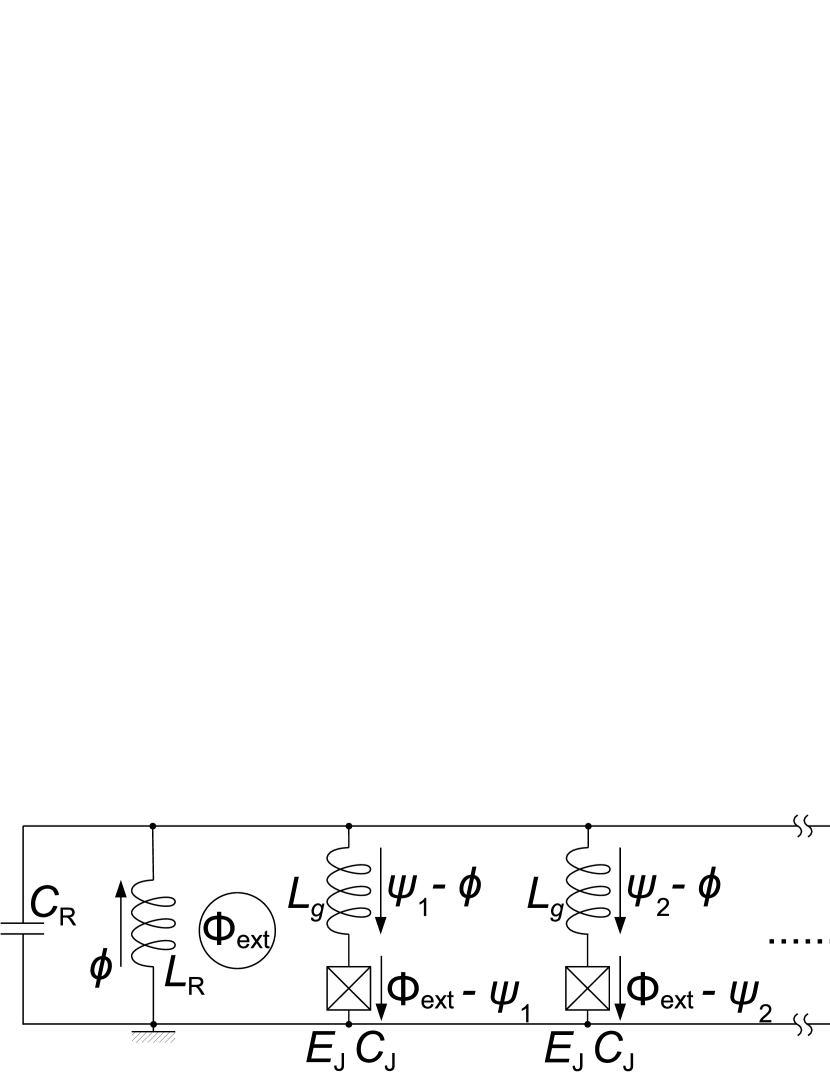
Figure 1: Superconducting circuit showing the SRPT in thermal equilibrium under a static external magnetic flux bias $\Phi_{\text{ext}}=\Phi_{0}/2$.

The circuit shown in Fig. 1 has a LC resonator with capacitance $C_{\text{R}}$ and inductance $L_{\text{R}}$, coupled to $N$ parallel branches containing a Josephson junction. Each junction has Josephson energy $E_{\text{J}}$ and shunt capacitance $C_{\text{J}}$ and is connected to the LC resonator through inductance $L_{{g}}$ individually. This configuration is distinct from the conventional inductive Jaako2016PRA ; Nataf2010PRL and capacitive couplings Jaako2016PRA , where the existence of the SRPT was proposed Nataf2010NC ; Ciuti2012PRL but was denied afterward Viehmann2011PRL ; Jaako2016PRA . However, the no-go result was shown only for such specific configurations Viehmann2011PRL ; Jaako2016PRA and is not applied to ours. We first explain why the SRPT occurs in our circuit by analyzing the form of the Hamiltonian.

We apply a static external flux bias $\Phi_{\text{ext}}=\Phi_{0}/2$ in the loop between the resonator and the junctions, where $\Phi_{0}=h/(2e)$ is the flux quantum. Alternatively, we can remove the external field and replace the Josephson junctions with $\pi$ junctions which have an inverted energy-phase relation Ryazanov2001PRL . We define the ground and the branch fluxes $\phi$ and $\{\psi_{j}\}$ ($j=1,\ldots,N$) as in Fig. 1. According to the flux-based procedure Devoret1997 , the Hamiltonian is derived straightforwardly and quantized as

$$\hat{H}=\frac{\hat{q}^{2}}{2C_{\text{R}}}+\frac{\hat{\phi}^{2}}{2L_{\text{R}}}+\sum_{j=1}^{N}\left[\frac{\hat{\rho}_{j}{}^{2}}{2C_{\text{J}}}+\frac{(\hat{\psi}_{j}-\hat{\phi})^{2}}{2L_{{g}}}+E_{\text{J}}\cos\frac{2\pi\hat{\psi}_{j}}{\Phi_{0}}\right].$$ (1)

Here, $\hat{q}$ and $\{\hat{\rho}_{j}\}$ are the conjugate momenta of $\hat{\phi}$ and $\{\hat{\psi}_{j}\}$, respectively, satisfying $[\hat{\phi},\hat{q}]=\mathrm{i}\hbar$ and $[\hat{\psi}_{j},\hat{\rho}_{j^{\prime}}]=\mathrm{i}\hbar\delta_{j,j^{\prime}}$.

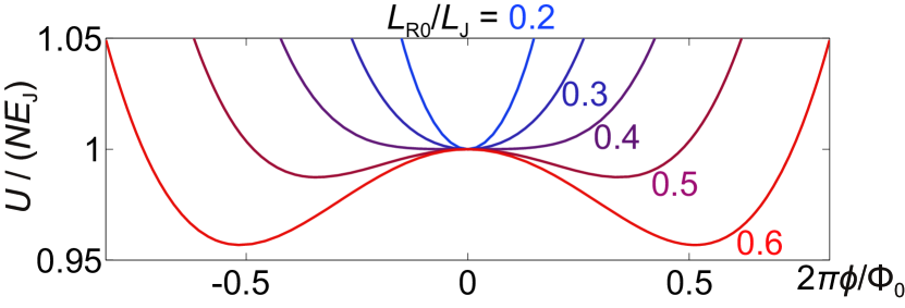
Figure 2: Normalized inductive energy [Eq. (2)] versus $2\pi\phi/\Phi_{0}$ under the condition of $\psi_{j}=(1+L_{{g}}/L_{\text{R}0})\phi$, which is obtained by $\partial{}U/\partial\phi=0$. For $NL_{\text{R}}=L_{\text{R}0}>L_{\text{J}}-L_{{g}}$, the inductive energy shows two minima at $\phi\neq 0$. This transition corresponds to the SRPT in the sense of the quantum phase transition. Parameter: $L_{{g}}=0.6L_{\text{J}}$.

Let us first understand intuitively the SRPT in our circuit by a classical analysis. The inductive energy in Eq. (1) is extracted as

$$U(\phi,\{\psi_{j}\})=\frac{\phi^{2}}{2L_{\text{R}}}+\sum_{j=1}^{N}\left[\frac{(\psi_{j}-\phi)^{2}}{2L_{{g}}}+E_{\text{J}}\cos\frac{2\pi\psi_{j}}{\Phi_{0}}\right].$$ (2)

The energy minima correspond to the ground state in the classical physics. While the parabolic terms $\phi^{2}/(2L_{\text{R}})$ and $(\psi_{j}-\phi)^{2}/(2L_{{g}})$ are minimized at $\phi=\psi_{j}=0$, the anharmonic term $E_{\text{J}}\cos(2\pi\psi_{j}/\Phi_{0})$ is minimized at $\psi_{j}=\pm\Phi_{0}/2$. This is owing to the external flux bias $\Phi_{\text{ext}}=\Phi_{0}/2$; the sign of the last term in Eqs. (1) and (2) is positive, because the phase difference across the Josephson junction is given by $\pi-2\pi(\psi_{j}/\Phi_{0})$ due to the flux quantization in each loop consisting of $L_{\text{R}}$, $L_{{g}}$, and the junction. This competition between the parabolic and anharmonic inductive energies is the trick for realizing the SRPT.

For simplifying the following discussion, we define an inductance $L_{\text{J}}\equiv[\Phi_{0}/(2\pi)]^{2}/E_{\text{J}}$ by the Josephson energy $E_{\text{J}}$. The inductive energy $U$ in Eq. (2) is minimized for $\psi_{j}=[1+L_{{g}}/(NL_{\text{R}})]\phi$, which is obtained from $\partial{}U/\partial\phi=0$. Since the SRPT is basically discussed in the thermodynamic limit $N\to\infty$, we scale the inductance of the LC resonator by the number $N$ of junctions as

$$L_{\text{R}}=L_{\text{R}0}/N,$$ (3)

where $L_{\text{R}0}$ is $N$-independent inductance. Then, the inductive energy $U/N$ per junction becomes independent of $N$. In Fig. 2, we plot $U/(NE_{\text{J}})$ as a function of $2\pi\phi/\Phi_{0}$ under the condition of $\psi_{j}=(1+L_{{g}}/L_{\text{R}0})\phi$. The five curves in Fig. 2 are the results for different $L_{\text{R}0}$ under a fixed $L_{{g}}$ of $0.6L_{\text{J}}$. The inductive energy $U$ is minimized at $\phi=\psi_{j}=0$ for $L_{\text{R}0}<L_{\text{J}}-L_{{g}}=0.4L_{\text{J}}$, since the parabolic terms dominate. In contrast, the anharmonic term dominates when $L_{\text{R}0}$ satisfies

$$NL_{\text{R}}=L_{\text{R}0}>L_{\text{J}}-L_{{g}}.$$ (4)

Then, $U$ is minimized at the two points with non-zero fluxes $\phi=\pm\phi_{\text{0}}$. In the quantum theory, the real ground state is a superposition of the two minimum points (conceptually speaking, $|\text{g}\rangle=\frac{|\phi_{\text{0}}\rangle+|-\phi_{\text{0}}\rangle}{\sqrt{2}}$) and the expectation values of the fluxes are zero $\langle\text{g}|\hat{\phi}|\text{g}\rangle=\langle\text{g}|\hat{\psi}_{j}|\text{g}\rangle=0$ for finite $N$. However, the thermodynamic limit $N\to\infty$ justifies the classical approach, since the height of the potential barrier in the whole system is proportional to $N$. Then, in this limit, we find a spontaneous appearance of coherence (symmetry breaking), i.e., non-zero $\phi=\pm\phi_{0}$ and $\psi_{j}=\pm(1+L_{{g}}/L_{\text{R}0})\phi_{0}$ appear in the circuit. This transition from $\phi=0$ to $\pm\phi_{\text{0}}$ by changing $L_{\text{R}0}$ corresponds to the SRPT in the sense of the quantum phase transition Emary2003PRL ; Emary2003PRE as discussed below in a quantum analysis.

Let us compare Eq. (1) with the minimal-coupling Hamiltonian (under the long-wavelength approximation as discussed in Ref. Bialynicki-Birula1979PRA )

$$\hat{H}_{\text{min}}=\hat{H}_{\text{em}}+\sum_{j}^{N}\frac{(\hat{p}_{j}-e\hat{A})^{2}}{2m}+\hat{V}(\{\hat{x}_{j}\}).$$ (5)

Here, $\hat{H}_{\text{em}}$ represents the energy of the transverse electromagnetic fields described by the vector potential $\hat{A}$ and its conjugate momentum. The second and the last terms are, respectively, the kinetic and the Coulomb interaction energies of particles with mass $m$, charge $e$, and momentum $\{\hat{p}_{j}\}$ at position $\{\hat{x}_{j}\}$. The kinetic energy $(\hat{p}_{j}-e\hat{A})^{2}/(2m)$ corresponds to the inductive one $(\hat{\psi}_{j}-\hat{\phi})^{2}/(2L_{{g}})$ at $L_{{g}}$ in Eq. (1). In this way, $\hat{\psi}_{j}$ and $\hat{\phi}$ correspond to $\hat{p}_{j}$ and $\hat{A}$, respectively, and then $\hat{\rho}_{j}$ corresponds to $\hat{x}_{j}$. The no-go theorem of the SRPT in the minimal-coupling Hamiltonian relies on the fact that the mixing term $(\hat{p}_{j}-e\hat{A})^{2}/(2m)$ and the anharmonic term $\hat{V}(\{\hat{x}_{j}\})$ are, respectively, described by $\hat{p}_{j}$ and $\hat{x}_{j}$ Bialynicki-Birula1979PRA ; Gawedzki1981PRA . In contrast, in our Hamiltonian, Eq. (1), both the mixing $(\hat{\psi}_{j}-\hat{\phi})^{2}/(2L_{{g}})$ and the anharmonicity $E_{\text{J}}\cos(2\pi\hat{\psi}_{j}/\Phi_{0})$ are described by $\hat{\psi}_{j}$. This is the essence for avoiding the no-go theorem Bialynicki-Birula1979PRA ; Gawedzki1981PRA and also for the transition discussed in the above classical analysis. In the Supplemental Material suppl , we also explain how we avoid the no-go results based on the $A^{2}$ term Rzazewski1975PRL ; Rzazewski1976PRA ; Yamanoi1976PLA ; Yamanoi1979JPA and on the $P^{2}$ one Emeljanov1976PLA ; Yamanoi1978P2 . The latter corresponds to the direct qubit-qubit interaction discussed recently in Ref. Jaako2016PRA .

By decomposing $\sum_{j=1}^{N}(\hat{\psi}_{j}-\hat{\phi})^{2}/(2L_{{g}})$ in Eq. (1), we obtain $N\hat{\phi}^{2}/(2L_{{g}})$. This corresponds to the $A^{2}$ term Rzazewski1975PRL ; Rzazewski1976PRA (since $\hat{\phi}$ corresponds to $\hat{A}$) and renormalizes the frequency of the LC resonator as $\omega_{\text{c}}=\sqrt{({N}/{L_{{g}}}+{1}/{L_{\text{R}}})/C_{\text{R}}}$. Here, in order to make $\omega_{\text{c}}$ independent of $N$, in addition to the scaling of $L_{\text{R}}$ in Eq. (3), we also scale the capacitance $C_{\text{R}}$ as

$$C_{\text{R}}=NC_{\text{R}0},$$ (6)

where $C_{\text{R}0}$ is $N$-independent capacitance. Introducing an annihilation operator $\hat{a}\equiv\hat{\phi}/\sqrt{2\hbar Z_{\text{c}}}+\mathrm{i}\hat{q}\sqrt{Z_{\text{c}}/(2\hbar)}$, where the impedance $Z_{\text{c}}$ is scaled as $Z_{\text{c}}=Z_{\text{c0}}/N$ for $Z_{\text{c0}}=\sqrt{({1}/{L_{{g}}}+{1}/{L_{\text{R}0}})^{-1}/C_{\text{R}0}}$, the Hamiltonian in Eq. (1) is rewritten as

$$\hat{H}=\hbar\omega_{\text{c}}\left(\hat{a}^{\dagger}\hat{a}+\frac{1}{2}\right)-\frac{\hat{\phi}}{L_{{g}}}\sum_{j=1}^{N}\hat{\psi}_{j}+\sum_{j=1}^{N}\hat{H}^{\text{atom}}_{j}.$$ (7)

Here, the Hamiltonian involving the $j$-th junction is

$$\hat{H}^{\text{atom}}_{j}=\frac{\hat{\rho}_{j}{}^{2}}{2C_{\text{J}}}+\frac{\hat{\psi}_{j}{}^{2}}{2L_{{g}}}+E_{\text{J}}\cos\frac{2\pi\hat{\psi}_{j}}{\Phi_{0}}.$$ (8)

Although we cannot obtain $\hat{H}^{\text{atom}}_{j}$ by simply extracting a part of elements from the circuit in Fig. 1, this anharmonic oscillator described by $\hat{\psi}_{j}$ and $\hat{\rho}_{j}$ is formally considered to be our “atom”. The first term in Eq. (7) is the Hamiltonian of our “photons”, which is described by $\hat{\phi}$ and $\hat{q}$ or $\hat{a}$, renormalized by the $A^{2}$ term. The second term in Eq. (7) is our “photon-atom interaction”. In the following, we discuss the SRPT in terms of these photons and atoms in relationship to the past discussions on the Dicke model Mallory1969PR ; Hepp1973AP ; Wang1973PRA ; Ciuti2012PRL ; Nataf2010NC ; Emary2003PRL ; Emary2003PRE .

In contrast to the two-level atoms considered in the Dicke model, our atoms have weakly-nonlinear bosonic transitions (we explain in detail the parameters used in the following calculations in the Supplemental Material suppl ). In Fig. 3(b), the solid curve represents the atomic wavefunction at each atomic level, which are calculated from $\hat{H}^{\text{atom}}_{j}$ in Eq. (8). The dashed curve represents the inductive energy as a function of $2\pi\psi_{j}/\Phi_{0}$. In this Letter, we basically consider the case $L_{\text{J}}>L_{{g}}=0.6L_{\text{J}}$. Then, since the anharmonic energy $E_{\text{J}}\cos(2\pi\psi_{j}/\Phi_{0})$ is smaller than the parabolic one $\psi_{j}{}^{2}/(2L_{{g}})$, as seen in Fig. 3(b), the inductive energy in each atom is minimized at $\psi_{j}=0$, and the nonlinearity is only about $3\%$.

Here, we tentatively neglect the anharmonicity as $E_{\text{J}}\cos(2\pi\hat{\psi}_{j}/\Phi_{0})\simeq E_{\text{J}}-\hat{\psi}_{j}{}^{2}/(2L_{\text{J}})$ and assume that the transitions in each atom are described approximately by bosonic annihilation operator $\hat{b}_{j}=\hat{\psi}_{j}/\sqrt{2\hbar Z_{\text{a}}}+\mathrm{i}\hat{\rho}_{j}\sqrt{Z_{\text{a}}/(2\hbar)}$ as

$$\hat{H} \simeq\hbar\omega_{\text{c}}\left(\hat{a}^{\dagger}\hat{a}+\frac{1}{2}\right)+\sum_{j=1}^{N}\hbar\omega_{\text{a}}\left(\hat{b}^{\dagger}_{j}\hat{b}_{j}+\frac{1}{2}\right)$$

$$\quad-\frac{\hbar g}{\sqrt{N}}(\hat{a}+\hat{a}^{\dagger})\sum_{j=1}^{N}(\hat{b}_{j}+\hat{b}^{\dagger}_{j})+NE_{\text{J}}.$$ (9)

Here, $\omega_{\text{a}}=\sqrt{({1}/{L_{{g}}}-{1}/{L_{\text{J}}})/C_{\text{J}}}$ is the atomic transition frequency, and the interaction strength $g$ is expressed as $g={\sqrt{NZ_{\text{c}}Z_{\text{a}}}}/{2L_{{g}}}={\sqrt{Z_{\text{c0}}Z_{\text{a}}}}/{2L_{{g}}}$, where we define another impedance $Z_{\text{a}}=\sqrt{({1}/{L_{{g}}}-{1}/{L_{\text{J}}})^{-1}/C_{\text{J}}}$.

Two transition frequencies $\omega_{\pm}$ of the bosonized Hamiltonian in Eq. (Super-radiant phase transition in superconducting circuit in thermal equilibrium) are obtained easily by the Bogoliubov transformation hopfield58 ; Ciuti2005PRB as

$$\omega_{\pm}{}^{2}=\frac{\omega_{\text{c}}{}^{2}+\omega_{\text{a}}{}^{2}\pm\sqrt{(\omega_{\text{c}}{}^{2}-\omega_{\text{a}}{}^{2})^{2}+16g^{2}\omega_{\text{c}}\omega_{\text{a}}}}{2}.$$ (10)

Note that $\omega_{\text{c}}$, $\omega_{\text{a}}$, $g$, and $\omega_{\pm}$ are not scaled with $N$ by the scaling of $L_{\text{R}}$ and $C_{\text{R}}$ in Eqs. (3) and (6), respectively. The expression in Eq. (10) is exactly the same as the one derived in the Holstein-Primakoff approach for the Dicke model Emary2003PRL ; Emary2003PRE . When $\omega_{-}$ becomes imaginary, the normal ground state (showing $\langle\text{g}|\hat{a}|\text{g}\rangle=\langle\text{g}|\hat{\phi}|\text{g}\rangle=0$) becomes unstable. However, it is an artifact due to the neglect of the anharmonicity in Eq. (Super-radiant phase transition in superconducting circuit in thermal equilibrium). As found in the classical analysis in Fig. 2, the real ground state appears at an inductive energy minimum with $\phi=\pm\phi_{0}$ (super-radiant ground state with a photonic amplitude of $\langle\text{g}|\hat{a}|\text{g}\rangle\simeq\pm\phi_{0}/\sqrt{2\hbar Z_{\text{c}}}$) in the presence of the anharmonicity Yamanoi1976PLA ; Yamanoi1979JPA ; Emary2003PRL ; Emary2003PRE ; Bamba2014SPT . Equation (10) suggests that the super-radiant ground state appears for $4g^{2}>\omega_{\text{c}}\omega_{\text{a}}$, which gives exactly the same condition as Eq. (4) obtained by the classical approach. While these conditions are certainly satisfied in our circuit, we will obtain a more rigorous condition of the SRPT in the following semi-classical analysis.

The above classical and bosonic quantum analyses imply the SRPT in the sense of the quantum phase transition, i.e., in the limit of $T\to 0$. On the other hand, the thermodynamic properties at a finite temperature $T$ is analyzed by the partition function $\mathcal{Z}(T)=\mathrm{Tr}[\mathrm{e}^{-\hat{H}/k_{\text{B}}T}]$. Since we have only one photonic mode in our system, in the thermodynamic limit $N\to\infty$, the trace over the photonic states can be replaced by the integral over the coherent state Wang1973PRA ; Hepp1973PRA ; Bialynicki-Birula1979PRA ; Hemmen1980PLA ; Gawedzki1981PRA (see also the Supplemental Material suppl ) as

$$\mathcal{Z}(T)\simeq\int\frac{\mathrm{d}^{2}\alpha}{\pi}\ \mathrm{e}^{-{\hbar\omega_{\text{c}}(|\alpha|^{2}+1/2)}/{k_{\text{B}}T}}\mathcal{Z}_{\text{atom}}(\alpha,T)^{N}.$$ (11)

Here, $\alpha\in\mathbb{C}$ is the amplitude of the coherent state $|\alpha\rangle$ giving $\hat{a}|\alpha\rangle=\alpha|\alpha\rangle$. The atomic partition function $\mathcal{Z}_{\text{atom}}(\alpha,T)=\mathrm{Tr}_{j}[\mathrm{e}^{-\hat{H}^{\text{eff}}_{j}(\alpha)/k_{\text{B}}{}T}]$ is defined with an effective Hamiltonian for a given $\alpha$ as

$$\hat{H}^{\text{eff}}_{j}(\alpha)=-\frac{1}{L_{{g}}}\phi(\alpha)\hat{\psi}_{j}+\hat{H}^{\text{atom}}_{j},$$ (12)

where the flux amplitude is expressed as $\phi(\alpha)=\sqrt{2\hbar Z_{\text{c}}}\mathrm{Re}[\alpha]=\sqrt{2\hbar Z_{\text{c0}}}\mathrm{Re}[\alpha]/\sqrt{N}$. The partition function in Eq. (11) is rewritten as $\mathcal{Z}(T)\simeq\int({\mathrm{d}^{2}\alpha}/{\pi})\mathrm{e}^{-S(\alpha,T)/k_{\text{B}}{}T}$, where the action is expressed as $S(\alpha,T)=\hbar\omega_{\text{c}}(|\alpha|^{2}+1/2)-Nk_{\text{B}}{}T\ln\mathcal{Z}_{\text{atom}}(\alpha,T)$. Since the photon-atom interaction is mediated by $\phi(\alpha)$ in Eq. (12), the minimum action is obtained for $\alpha\in\mathbb{R}$. Then, the photonic amplitude $\alpha_{\text{eq}}$ in the thermal equilibrium at $T$ is determined by $\mathrm{d}{}S(\alpha,T)/\mathrm{d}\alpha=0$, which is rewritten as

$$\left(\frac{1}{L_{\text{R}0}}+\frac{1}{L_{{g}}}\right)\phi_{\text{eq}}-\frac{1}{L_{{g}}}\frac{\mathrm{Tr}\left[\hat{\psi}_{j}\mathrm{e}^{-\hat{H}^{\text{eff}}_{j}(\alpha_{\text{eq}})/k_{\text{B}}T}\right]}{\mathcal{Z}_{\text{atom}}(\alpha_{\text{eq}},T)}=0,$$ (13)

where $\phi_{\text{eq}}=\phi(\alpha_{\text{eq}})$ is the flux amplitude.

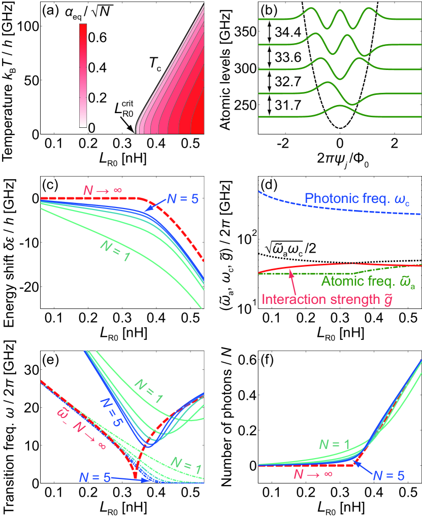
Figure 3: (a) Normalized photonic amplitude $\alpha_{\text{eq}}/\sqrt{N}$ in the thermodynamic limit (infinite number of atoms $N\to\infty$) versus $L_{\text{R}0}=NL_{\text{R}}$ and temperature $k_{\text{B}}T/h$ in frequency unit. The SRPT occurs at $L_{\text{R}0}^{\text{crit}}$ at $T=0$. (b) Atomic levels, potential, and wavefunctions. (c) Zero-point energy shift, (e) transition frequency, and (f) number of photons per atom versus $L_{\text{R}0}$. Dashed curves are obtained in the thermodynamic limit, and solid curves are calculated for $N=1,\ldots,5$. In (e), the dash-dotted curves represent the transition frequencies for exciting odd number of bosons, while the solid curves are those for exciting even number of bosons. (d) Photonic frequency $\omega_{\text{c}}$, renormalized atomic frequency $\tilde{\omega}_{\text{a}}$, and renormalized light-matter interaction strength $\tilde{g}$ versus $L_{\text{R}0}$. The SRPT occurs when $\tilde{g}$ reaches the critical interaction strength $\sqrt{\tilde{\omega}_{\text{a}}\omega_{\text{c}}}/2$ plotted by the dotted line. Parameters: $L_{\text{J}}=0.75\;\mathrm{nH}$, $L_{{g}}=0.6L_{\text{J}}=0.45\;\mathrm{nH}$, $C_{\text{J}}=24\;\mathrm{fF}$, and $C_{\text{R}0}=2\;\mathrm{fF}=C_{\text{R}}/N$.

In Fig. 3(a), the normalized photonic amplitude $\alpha_{\text{eq}}/\sqrt{N}$ calculated by Eq. (13) is color-plotted as a function of the inductance $L_{\text{R}0}=NL_{\text{R}}$ and temperature $k_{\text{B}}T/h$ in frequency unit. What is important is the ratio of the inductances. The Josephson inductance is assumed to be $L_{\text{J}}=[\Phi_{0}/(2\pi)]^{2}/E_{\text{J}}=0.75\;\mathrm{nH}$, and the connecting inductance $L_{{g}}=0.6L_{\text{J}}=0.45\;\mathrm{nH}$. At $T=0$, the non-zero photonic amplitude $\alpha_{\text{eq}}$ appears for $L_{\text{R}0}>L_{\text{R}0}^{\text{crit}}\simeq 0.34\;\mathrm{nH}$, which roughly agrees with the classical result $L_{\text{J}}-L_{{g}}=0.30\;\mathrm{nH}$ in Eq. (4). The deviation is due to the quantum treatment of atoms in Eq. (13). The photonic flux $\phi_{\text{eq}}$ roughly agrees with $\phi_{0}$ giving the minimum of the inductive energy $U$ in Eq. (2) in the classical analysis. The non-zero $\alpha_{\text{eq}}$ and $\phi_{\text{eq}}$ appear even at finite temperatures, and the critical temperature $T_{\text{c}}$ increases with increasing $L_{\text{R}0}$. This is the main evidence of the thermal-equilibrium SRPT in our circuit, which is obtained in the thermodynamic limit $N\to\infty$.

The transition frequencies, which are experimentally observable, are obtained by quantizing the fluctuation around the equilibrium value $\phi_{\text{eq}}$ determined by Eq. (13). A similar analysis has been performed in Refs. Emary2003PRL ; Emary2003PRE for the Dicke Hamiltonian. The atomic flux at $T=0$ is determined as the expectation value $\psi_{\text{eq}}=\langle\hat{\psi}_{j}\rangle_{\text{g}}^{\text{eff}}$ in the ground state of the effective Hamiltonian $\hat{H}^{\text{eff}}_{j}(\alpha_{\text{eq}})$. The original Hamiltonian in Eq. (1) is expanded with respect to the fluctuations $\delta\hat{\phi}=\hat{\phi}-\phi_{\text{eq}}$ and $\delta\hat{\psi}_{j}=\hat{\psi}_{j}-\psi_{\text{eq}}$ up to $O(\delta\hat{\psi}_{j}{}^{2})$ suppl as

$$\hat{H} \simeq\frac{\hat{q}^{2}}{2C_{\text{R}}}+\frac{\delta\hat{\phi}^{2}}{2L_{\text{R}}}+\sum_{j=1}^{N}\left\{\frac{\hat{\rho}^{2}}{2C_{\text{J}}}+\frac{(\delta\hat{\phi}-\delta\hat{\psi}_{j})^{2}}{2L_{{g}}}-\frac{\delta\hat{\psi}_{j}{}^{2}}{2\tilde{L}_{\text{J}}}\right\}$$

$$\quad+N(E_{\text{J}}+\delta\varepsilon).$$ (14)

Here, $\tilde{E}_{\text{J}}=E_{\text{J}}\langle\cos(2\pi\hat{\psi}/\Phi_{0})\rangle_{\text{g}}^{\text{eff}}$ and $\tilde{L}_{\text{J}}=[\Phi_{0}/(2\pi)]^{2}/\tilde{E}_{\text{J}}$ are modified by the quantum treatment of atoms even before the SRPT. The zero-point energy shift per atom is

$$\delta\varepsilon=\frac{\phi_{\text{eq}}{}^{2}}{2L_{\text{R}0}}+\frac{(\phi_{\text{eq}}-\psi_{\text{eq}})^{2}}{2L_{{g}}}+\tilde{E}_{\text{J}}-E_{\text{J}}.$$ (15)

This shift $\delta\varepsilon/h$ is plotted as the dashed curve in Fig. 3(c). After the appearance of non-zero amplitudes $\phi_{\text{eq}}$ and $\psi_{\text{eq}}$, the zero-point energy is decreased by the light-matter interaction.

The transition frequencies $\tilde{\omega}_{\pm}$ are calculated also from Eq. (10) but with replacing $\omega_{\text{a}}$ and $g$ by $\tilde{\omega}_{\text{a}}=[({1}/{L_{{g}}}-{1}/{\tilde{L}_{\text{J}}})/C_{\text{J}}]^{1/2}$ and $\tilde{g}={[Z_{\text{c0}}\tilde{Z}_{\text{a}}}]^{1/2}/{(2L_{{g}})}$, respectively, where $\tilde{Z}_{\text{a}}=[({1}/{L_{{g}}}-{1}/{\tilde{L}_{\text{J}}})^{-1}/C_{\text{J}}]^{1/2}$. $\tilde{\omega}_{\text{a}}$, $\omega_{\text{c}}$, and $\tilde{g}$ are plotted in Fig. 3(d). When $\tilde{g}$ reaches the critical value $\sqrt{\tilde{\omega}_{\text{a}}\omega_{\text{c}}}/2$ plotted by the dotted line, the SRPT occurs. Compared with the simple condition $4g^{2}>\omega_{\text{c}}\omega_{\text{a}}$ (giving the critical inductance $L_{\text{J}}-L_{{g}}=0.30\;\mathrm{nH}$) obtained from Eq. (Super-radiant phase transition in superconducting circuit in thermal equilibrium) under the bosonic approximation, the deviation is due to the consideration of the anharmonicity in Eq. (Super-radiant phase transition in superconducting circuit in thermal equilibrium). The lower transition frequency $\tilde{\omega}_{-}$ is plotted by the dashed line in Fig. 3(e). It never becomes imaginary value but shows a cusp at $L_{\text{R}0}^{\text{crit}}$. In contrast to the Dicke model Emary2003PRL ; Emary2003PRE , $\tilde{\omega}_{-}$ does not become zero even at $L_{\text{R}0}^{\text{crit}}$ in our system. It is due to the presence of multiple atomic levels with anharmonicity (our atom cannot be equivalent with the two-level limit since $L_{\text{J}}>L_{{g}}$ is required). On the other hand, in the limit of negligible anharmonicity ($L_{\text{J}}\gg L_{{g}}$), the SRPT condition in Eq. (4) is justified, and $\tilde{\omega}_{-}$ drops to zero at $L_{\text{R}0}^{\text{crit}}$.

Here, we note that, in the limit of $L_{{g}}\to 0$, we definitively get $\psi_{j}=\phi$ as seen in Eq. (1) or in the circuit of Fig. 1, while the transition in Fig. 2 itself occurs in the classical approach. We also get $\omega_{\text{a}},g\to\infty$, while $4g^{2}>\omega_{\text{c}}\omega_{\text{a}}$ is reduced to $L_{\text{R}0}>L_{\text{J}}$, and the transition still remains. However, in order to distinguish the photons and atoms and to discuss the SRPT, we need a finite $L_{{g}}$. Especially, as far as we checked numerically, $L_{\text{R}0}$, $L_{\text{J}}$, and $L_{{g}}$ are desired to be in the same order to observe a sharp drop of the transition frequency for finite $N$ as we will see in the following.

In addition to the above semi-classical approach justified in the thermodynamic limit $N\to\infty$, we also diagonalize numerically the original Hamiltonian in Eq. (7) for $N=1,2,\ldots,5$ in order to predict the tendency to be observed in experiments with a finite number of junctions. For expressing the Hamiltonian with a sparse matrix and reducing the computational cost, we expand $\cos(2\pi\hat{\psi}_{j}/\Phi_{0})$ and consider the terms up to $O(\hat{\psi}_{j}{}^{4})$ (see the details of the numerical diagonalization in the Supplemental Material suppl ).

Since the total Hamiltonian in Eq. (1) or (7) has the parity symmetry, the expectation value of the photonic amplitude in the ground state is basically zero for finite $N$. The non-zero $\alpha_{\text{eq}}$ is obtained only in the thermodynamic limit $N\to\infty$. In the numerical diagonalization of the Hamiltonian, we first consider the subsystem with even numbers of bosons as in Ref. Emary2003PRE , because it is not mixed with the other subsystem with odd numbers of bosons. For the obtained ground state $|\text{g}\rangle$ with an energy $E_{\text{g}}$, the expectation number of photons $\langle\text{g}|\hat{a}^{\dagger}\hat{a}|\text{g}\rangle/N$ per atom is plotted in Fig. 3(f) for $N=1,\ldots,5$. The dashed curve shows $\alpha_{\text{eq}}{}^{2}/N$ in the thermodynamic limit. Figure 3(c) shows the zero-point energy shift $\delta\varepsilon=(E_{\text{g}}-\hbar\omega_{\text{c}}/2)/N-\varepsilon_{\text{a}0}$ per atom, where $\varepsilon_{\text{a}0}$ is the atomic zero-point energy seen in Fig. 3(b). The transition frequency from the ground state to the first excited state in the even-number subsystem is plotted as solid curves in Fig. 3(e). It sharply drops around $L_{\text{R}0}^{\text{crit}}$ even with $N=5$ atoms and asymptotically reproduces the thermodynamic limit (dashed curve) for $L_{\text{R}0}>L_{\text{R}0}^{\text{crit}}$. On the other hand, the dash-dotted curves represent the transition frequency from the ground state to the lowest state in the odd-number subsystem. They asymptotically approach the thermodynamic limit for $L_{\text{R}0}<L_{\text{R}0}^{\text{crit}}$ and vanish for $L_{\text{R}0}>L_{\text{R}0}^{\text{crit}}$ as seen also in Refs. Emary2003PRE ; Nataf2010PRL . These characteristic features imply the existence of the SRPT, i.e., the parity symmetry breaking Emary2003PRL ; Emary2003PRE .

We conclude that the superconducting circuit in Fig. 1 shows the SRPT in the thermal equilibrium. It was confirmed by the semi-classical approach in the thermodynamic limit. It was also checked by calculating the number of photons, transition frequency, and zero-point energy shift in the numerical diagonalization of the Hamiltonian with a finite number of atoms. Experimentally, the transition frequency could be observed by measuring the excitation spectra, which would reveal a drastic behavior around the critical point, as seen in Fig. 3(e), by changing $L_{\text{R}0}$, by decreasing the temperature, or by increasing the number of atoms.

Supplemental Material

In the main text, we explain why the SRPT occurs in our circuit by analyzing the form of the Hamiltonian, i.e., we show that the transition of the inductive energy minima corresponds to the SRPT and that the anharmonic term described by $\hat{\psi}_{j}$ is essential in our SRPT. While we consider that they are the most intuitive and general explanations, we also explain how we avoid the no-go results based on the $A^{2}$ term in Appendix A and on the $P^{2}$ term in Appendix B, where we also show that the direct qubit-qubit interaction is obtained by a unitary transformation of our Hamiltonian and corresponds to the $P^{2}$ term. The justification of the semi-classical analysis is shown in Appendix C. The derivation of the effective Hamiltonian around the equilibrium is performed in Appendix D. In Appendix E, we show the details of the numerical diagonalization of the Hamiltonian for a finite number of junctions.

Appendix A Why the $A^{2}$ term does not prevent our SRPT

While the $A^{2}$ term prevents the SRPT in the atomic systems Rzazewski1975PRL ; Rzazewski1976PRA ; Yamanoi1976PLA ; Yamanoi1979JPA and also in the superconducting circuits with the conventional capacitive coupling Viehmann2011PRL , it does not prevent it in our system. Here we explain how we avoid the no-go result based on the $A^{2}$ term. In our Hamiltonian, the inductive energy at $L_{{g}}$ is expanded as

$$\sum_{j=1}^{N}\frac{(\hat{\psi}_{j}-\hat{\phi})^{2}}{2L_{{g}}}=\frac{N\hat{\phi}^{2}}{2L_{{g}}}-\sum_{j=1}^{N}\frac{\hat{\phi}\hat{\psi}_{j}}{L_{{g}}}+\sum_{j=1}^{N}\frac{\hat{\psi}_{j}{}^{2}}{2L_{{g}}}.$$ (16)

The first term is the $A^{2}$ term, and the second term represents the photon-atom interaction. The third term is a part of the atomic Hamiltonian as

$$\hat{H}^{\text{atom}}_{j}=\frac{\hat{\rho}_{j}{}^{2}}{2C_{\text{J}}}+\frac{\hat{\psi}_{j}{}^{2}}{2L_{{g}}}+E_{\text{J}}\cos\frac{2\pi\hat{\psi}_{j}}{\Phi_{0}}.$$ (17)

As discussed in the main text, $\hat{\psi}_{j}{}^{2}/(2L_{{g}})$ corresponds to the kinetic energy $\hat{p}_{j}{}^{2}/(2m)$ of charged particles. The essential difference from the minimal-coupling Hamiltonian is that our atomic Hamiltonian in Eq. (17) has the anharmonic term $E_{\text{J}}\cos(2\pi\hat{\psi}_{j}/\Phi_{0})$ described by $\hat{\psi}_{j}$ as we also mention in the main text. As the result, our particle mass $L_{{g}}$ is effectively increased to $(1/L_{{g}}-1/L_{\text{J}})^{-1}$ owing to the anharmonic term. Then, the atomic transition frequency

$$\omega_{\text{a}}=\sqrt{({1}/{L_{{g}}}-{1}/{L_{\text{J}}})/C_{\text{J}}}$$ (18)

is lowered and the interaction strength

$$g=\sqrt{Z_{\text{c0}}\sqrt{({1}/{L_{{g}}}-{1}/{L_{\text{J}}})^{-1}/C_{\text{J}}}}/{(2L_{{g}})}$$ (19)

is increased, compared respectively with $\sqrt{1/(L_{{g}}C_{\text{J}})}$ and $\sqrt{Z_{\text{c0}}\sqrt{L_{{g}}/C_{\text{J}}}}/{(2L_{{g}})}$ obtained in the absence of the anharmonic term. In contrast, the $A^{2}$ term $N\hat{\phi}^{2}/2L_{{g}}$ and $\omega_{\text{c}}$ are not modified by the anharmonic term. As a result, the interaction strength $g$ can exceed the critical value $\sqrt{\omega_{\text{c}}\omega_{\text{a}}}/2$ for the SRPT in our system. This is the reason why the $A^{2}$ term does not prevent our SRPT.

Appendix B Direct junction-junction interaction and the SRPT

The absence of SRPT in the superconducting circuits with the conventional capacitive coupling was discussed in terms of the direct qubit-qubit interaction in Ref. Jaako2016PRA , which corresponds to the $P^{2}$ term Emeljanov1976PLA ; Yamanoi1978P2 in the atomic systems as we will explain later. In the same manner as the unitary transformation between the Hamiltonians with the $A^{2}$ and the $P^{2}$ terms Keeling2007JPCM ; Bamba2014SPT , we can transform our Hamiltonian to another expression with a direct junction-junction interaction as in Ref. Jaako2016PRA .

By introducing a unitary operator

$$\hat{U}=\exp\left(\frac{1}{\mathrm{i}\hbar}\hat{\phi}\sum_{j=1}^{N}\hat{\rho}_{j}\right),$$ (20)

the flux $\hat{\psi}_{j}$ in each junction and the charge $\hat{q}$ in the LC resonator are transformed as

$$\hat{U}^{\dagger}\hat{\psi}_{j}\hat{U} =\hat{\psi}_{j}+\hat{\phi},$$ (21a)

$$\hat{U}^{\dagger}\hat{q}\hat{U} =\hat{q}-\sum_{j=1}^{N}\hat{\rho}_{j}.$$ (21b)

Then, our Hamiltonian is transformed as

$$\hat{U}^{\dagger}\hat{H}\hat{U} =\frac{1}{2C_{\text{R}}}\left(\hat{q}-\sum_{j=1}^{N}\hat{\rho}_{j}\right)^{2}+\frac{\hat{\phi}^{2}}{2L_{\text{R}}}$$

$$\quad+\sum_{j=1}^{N}\left[\frac{\hat{\rho}_{j}{}^{2}}{2C_{\text{J}}}+\frac{\hat{\psi}_{j}}{2L_{{g}}}+E_{\text{J}}\cos\frac{2\pi(\hat{\psi}_{j}+\hat{\phi})}{\Phi_{0}}\right].$$ (22)

Expanding the first term, we get $\sum_{j,j^{\prime}}\hat{\rho}_{j}\hat{\rho}_{j^{\prime}}/(2C_{\text{R}})$, which corresponds to the direct qubit-qubit interaction discussed in Ref. Jaako2016PRA . Further, since $\hat{\rho}_{j}$ corresponds to the position $\hat{x}_{j}$ of the charged particle, this term also corresponds to the $P^{2}$ term, the square of the electric polarization $\hat{P}(x)=\sum_{j}e\hat{x}_{j}\delta(x-\hat{x}_{j})$ in atomic systems as discussed in Refs. Emeljanov1976PLA ; Yamanoi1978P2 . In the same manner as the $A^{2}$ term, this $P^{2}$ term prevents the SRPT in atomic systems Emeljanov1976PLA ; Yamanoi1978P2 and also in superconducting circuits with the conventional capacitive coupling Jaako2016PRA .

However, since our Hamiltonian has the anharmonic term $E_{\text{J}}\cos(2\pi\hat{\psi}_{j}/\Phi_{0})$ described by $\hat{\psi}_{j}$, we get again the $A^{2}$ term (and also $A^{4}$, $A^{6}$, …terms) from the last term in Eq. (B) after the unitary transformation. As discussed in Refs. Knight1978PRA ; Keeling2007JPCM , the SRPT occurs in some Hamiltonians with both the $A^{2}$ and $P^{2}$ terms. While it is hard to compare Eq. (B) with the Hamiltonians in Refs. Knight1978PRA ; Keeling2007JPCM due to the presence of the $A^{4}$, $A^{6}$, …terms, the SRPT occurs in our system as discussed in the main text and also in Appendix A. In this way, the anharmonic term described by $\psi_{j}$ is essential for our SRPT.

Appendix C Justification of the semi-classical approach

In the semi-classical approach, we replace the trace over the photonic states by the integral over the coherent state in Eq. (11) of the main text. The justification of this replacement has been discussed in Refs. Wang1973PRA ; Hepp1973PRA ; Hemmen1980PLA ; Gawedzki1981PRA . In the early study by Wang and Hioe Wang1973PRA , they noted that this replacement is justified on the following two assumptions Wang1973PRA :

1. The limits as $N\rightarrow\infty$ of the field operator $\hat{a}/\sqrt{N}$ and $\hat{a}^{\dagger}/\sqrt{N}$ exist.

2. The order of the double limit in the exponential series $\lim_{N\rightarrow\infty}\lim_{R\rightarrow\infty}\sum_{r=1}^{R}(-\beta\hat{H})^{r}/r!$ can be interchanged.

The validities of these assumptions have been discussed for some atomic models including the case with a finite number of the electromagnetic modes Hepp1973PRA . While the first assumption seems to be satisfied since $\alpha_{\text{eq}}/\sqrt{N}$ ($\propto\phi_{\text{eq}}$) shows a finite value after the SRPT in the thermodynamic limit $N\to\infty$, it is hard to show whether our system satisfies the second assumption. Instead, we justify our semi-classical approach according to the discussion in Refs. Hepp1973PRA . The exact partition function $\mathcal{Z}(T)=\mathrm{Tr}[\mathrm{e}^{-\hat{H}/k_{\text{B}}T}]$ and the approximated one $\bar{\mathcal{Z}}(T)$ in Eq. (11) of the main text show the following relation Hepp1973PRA :

$$\bar{\mathcal{Z}}(T)\leq\mathcal{Z}(T)\leq\exp\left(\frac{1}{k_{\text{B}}T}\sum_{k=1}^{M}\hbar\omega_{k}\right)\bar{\mathcal{Z}}(T).$$ (23)

Here, we generally consider $M$ photonic modes with frequencies $\{\omega_{k}\}$, while our system has only $M=1$ mode with $\omega_{\text{c}}$. The free energy per atom is

$$-\frac{1}{N}\sum_{k=1}^{M}\hbar\omega_{k}-\frac{k_{\text{B}}T}{N}\ln\bar{\mathcal{Z}}(T)\\ \leq-\frac{k_{\text{B}}T}{N}\ln\mathcal{Z}(T)\leq-\frac{k_{\text{B}}T}{N}\ln\bar{\mathcal{Z}}(T).$$ (24)

Then, if the number $M$ of photonic modes is finite ($\lim_{N\to\infty}\sum_{k=1}^{M}\hbar\omega_{k}/N=0$), and the free energy $-({k_{\text{B}}T}/{N})\ln\bar{\mathcal{Z}}(T)$ per atom is also a finite value, $\mathcal{Z}(T)$ is well approximated by $\bar{\mathcal{Z}}(T)$ in the thermodynamic limit. In our case, we numerically checked that the free energy per atom $-(k_{\text{B}}T/N)\ln\bar{\mathcal{Z}}(T)$ converges to a finite value with increasing the number of atomic levels considered in the calculation. Thus, the replacement performed in Eq. (11) is justified.

Appendix D Deriving the effective Hamiltonian around equilibrium

For deriving the effective Hamiltonian around the equilibrium [Eq. (14) in the main text], we expand the anharmonic term in Eq. (1) of the main text up to $O[(\delta\hat{\psi}_{j}/\Phi_{0})^{2}]$ as

$$\cos(2\pi\hat{\psi}_{j}/\Phi_{0}) \simeq\langle\cos(2\pi\hat{\psi}_{j}/\Phi_{0})\rangle_{\text{g}}^{\text{eff}}[1-(2\pi\delta\hat{\psi}_{j}/\Phi_{0})^{2}/2]$$

$$\quad-\langle\sin(2\pi\hat{\psi}_{j}/\Phi_{0}]\rangle_{\text{g}}^{\text{eff}}(2\pi\delta\hat{\psi}_{j}/\Phi_{0}).$$ (25)

Further, we use $(1/L_{\text{R}0}+1/L_{{g}})\phi_{\text{eq}}-\psi_{\text{eq}}/L_{{g}}=0$ obtained from Eq. (13) at zero temperature and $(\psi_{\text{eq}}-\phi_{\text{eq}})/L_{{g}}-(2\pi/\Phi_{0})E_{\text{J}}\langle\sin(2\pi\hat{\psi}_{j}/\Phi_{0})\rangle_{\text{g}}^{\text{eff}}=0$ obtained from $[\hat{\rho}_{j},\hat{H}^{\text{eff}}_{j}(\alpha)]=0$.

Appendix E Numerical diagonalization of Hamiltonian for a finite number of junctions

For expressing the Hamiltonian with a sparse matrix and reducing the computational cost, the atomic Hamiltonian in Eq. (8) of the main text is approximated as

$$\hat{H}^{\text{atom}}_{j} \simeq\hbar\omega_{\text{a}}\left(\hat{b}^{\dagger}_{j}\hat{b}_{j}+\frac{1}{2}\right)+\frac{E_{\text{J}}}{4!}\left(\frac{2\pi\hat{\psi}_{j}}{\Phi_{0}}\right)^{4}+E_{\text{J}}.$$ (26)

Each atom is represented in the Fock basis up to 24 bosons, which is large enough since the expectation number of bosons is at most 3.25 under the parameters in Fig. 3 of the main text. The influence of this approximation (truncating higher Taylor series) was checked numerically. We found at most 1.5% difference between the lowest eight transition frequencies obtained for the original atomic Hamiltonian in Eq. (8) of the main text and for the approximated one in Eq. (26).

The parameters used in this study are chosen basically for the computational convenience, and we can choose other values without changing our results qualitatively. We find that $C_{\text{J}}=24\;\mathrm{fF}$, $L_{\text{J}}=0.75\;\mathrm{nH}$ ($E_{\text{J}}/h=218\;\mathrm{GHz}$), and $L_{{g}}=0.6L_{\text{J}}$ suppress sufficiently the expectation number of bosons in each atom and also the influence of the truncation performed in Eq. (26). These values are realized by a Josephson junction with an area of around $S=0.4\;\mathrm{\mu{}m}^{2}$ and a relatively large inductance structure for $L_{{g}}$. They were searched numerically under the restrictions that each atom is made by a Josephson junction and three inductances $L_{\text{J}}$, $L_{{g}}$, and $L_{\text{R}0}^{\text{crit}}$ are in the same order, by which the drop of the transition frequency is sharpened even for $N=5$ as seen in Fig. 3(e) of the main text. In order to suppress the expectation number of photons, we need to consider $\omega_{\text{c}}\gg\omega_{\text{a}}$. For this reason, we set $C_{\text{R}0}=2\;\mathrm{fF}$, while our results are not changed qualitatively even if $C_{\text{R}0}$ has a different magnitude.

In the numerical diagonalization of the Hamiltonian for the finite number of atoms under the truncation in Eq. (26), the maximum number of bosons is restricted to 48 in the whole system (and maximally 24 bosons in each mode) in both calculations for the even-number and odd-number subsystems. We numerically checked that the results converge sufficiently by this Fock basis.

We also calculated the transition frequencies for $N=1$ and 2 without the truncation (but the maximum number of bosons is only 16 in each mode due to the computational restriction). Note that the transition frequency from the ground state to the first excited state in the even-number subsystem [solid curves in Fig. 3(e) of the main text] clearly drops around the critical point even without the truncation. The difference between lowest values of the transition frequencies with and without the truncation is 6.0 % for $N=1$ and 4.2 % for $N=2$, and the difference between the optimal $L_{\text{R}0}$ (giving the lowest transition frequencies) with and without the truncation is 4.5 % for both $N=1$ and 2. In this way, the influence of the truncation on the lowest transition frequencies is suppressed at least by increasing $N$ from 1 to 2.

References

- (1) W. R. Mallory, Solution of a Multiatom Radiation Model Using the Bargmann Realization of the Radiation Field, Phys. Rev. 188, 1976 (1969).
- (2) K. Hepp and E. H. Lieb, On the superradiant phase transition for molecules in a quantized radiation field: the Dicke maser model, Ann. Phys. 76, 360 (1973).
- (3) Y. K. Wang and F. T. Hioe, Phase Transition in the Dicke Model of Superradiance, Phys. Rev. A 7, 831 (1973).
- (4) K. Rzążewski, K. Wódkiewicz, and W. Żakowicz, Phase Transitions, Two-Level Atoms, and the Term, Phys. Rev. Lett. 35, 432 (1975).
- (5) K. Rzążewski and K. Wódkiewicz, Thermodynamics of two-level atoms interacting with the continuum of electromagnetic field modes, Phys. Rev. A 13, 1967 (1976).
- (6) M. Yamanoi, Influence of omitting the term in the conventional photon-matter-Hamiltonian on the photon-field equation, Phys. Lett. A 58, 437 (1976).
- (7) M. Yamanoi, On polariton instability and thermodynamic phase transition in a photon-matter system, J. Phys. A 12, 1591 (1979).
- (8) I. Bialynicki-Birula and K. Rzążewski, No-go theorem concerning the superradiant phase transition in atomic systems, Phys. Rev. A 19, 301 (1979).
- (9) K. Gawȩdzki and K. Rzążewski, No-go theorem for the superradiant phase transition without dipole approximation, Phys. Rev. A 23, 2134 (1981).
- (10) F. Dimer, B. Estienne, A. S. Parkins, and H. J. Carmichael, Proposed realization of the Dicke-model quantum phase transition in an optical cavity QED system, Phys. Rev. A 75, 013804 (2007).
- (11) K. Baumann, C. Guerlin, F. Brennecke, and T. Esslinger, Dicke quantum phase transition with a superfluid gas in an optical cavity, Nature 464, 1301 (2010).
- (12) K. Baumann, R. Mottl, F. Brennecke, and T. Esslinger, Exploring Symmetry Breaking at the Dicke Quantum Phase Transition, Phys. Rev. Lett. 107, 140402 (2011).
- (13) P. Nataf and C. Ciuti, No-go theorem for superradiant quantum phase transitions in cavity QED and counter-example in circuit QED, Nat. Commun. 1, 72 (2010).
- (14) O. Viehmann, J. von Delft, and F. Marquardt, Superradiant Phase Transitions and the Standard Description of Circuit QED, Phys. Rev. Lett. 107, 113602 (2011).
- (15) C. Ciuti and P. Nataf, Comment on “Superradiant Phase Transitions and the Standard Description of Circuit QED”, Phys. Rev. Lett. 109, 179301 (2012).
- (16) T. Jaako, Z.-L. Xiang, J. J. Garcia-Ripoll, and P. Rabl, Ultrastrong-coupling phenomena beyond the Dicke model, Phys. Rev. A 94, 033850 (2016).
- (17) M. H. Devoret, Quantum fluctuations in electrical circuits, in Quantum fluctuations, Les Houches LXIII, 1995, edited by S. Reynaud, E. Giacobino, and J. Zinn-Justin (Elsevier, Amsterdam, 1997), Chap. 10, pp. 351–386.
- (18) K. Hepp and E. H. Lieb, Equilibrium Statistical Mechanics of Matter Interacting with the Quantized Radiation Field, Phys. Rev. A 8, 2517 (1973).
- (19) J. L. van Hemmen and K. Rzążewski, On the thermodynamic equivalence of the Dicke maser model and a certain spin system, Phys. Lett. A 77, 211 (1980).
- (20) P. Nataf and C. Ciuti, Vacuum Degeneracy of a Circuit QED System in the Ultrastrong Coupling Regime, Phys. Rev. Lett. 104, 023601 (2010).
- (21) V. V. Ryazanov, V. A. Oboznov, A. Y. Rusanov, A. V. Veretennikov, A. A. Golubov, and J. Aarts, Coupling of Two Superconductors through a Ferromagnet: Evidence for a Junction, Phys. Rev. Lett. 86, 2427 (2001).
- (22) C. Emary and T. Brandes, Quantum Chaos Triggered by Precursors of a Quantum Phase Transition: The Dicke Model, Phys. Rev. Lett. 90, 044101 (2003).
- (23) C. Emary and T. Brandes, Chaos and the quantum phase transition in the Dicke model, Phys. Rev. E 67, 066203 (2003).
- (24) See the Supplemental Material.
- (25) V. I. Emeljanov and Y. L. Klimontovich, Appearance of collective polarisation as a result of phase transition in an ensemble of two-level atoms, interacting through electromagnetic field, Phys. Lett. A 59, 366 (1976).
- (26) M. Yamanoi and M. Takatsuji, Influence of omitting the term in the multipole photon-matter Hamiltonian on the stability and propagation, in Coherence and quantum optics IV: Proceedings of the Fourth Rochester Conference on Coherence and Quantum Optics, edited by L. Mandel and E. Wolf (Plenum Press, New York, 1978), pp. 839–850.
- (27) J. J. Hopfield, Theory of the Contribution of Excitons to the Complex Dielectric Constant of Crystals, Phys. Rev. 112, 1555 (1958).
- (28) C. Ciuti, G. Bastard, and I. Carusotto, Quantum vacuum properties of the intersubband cavity polariton field, Phys. Rev. B 72, 115303 (2005).
- (29) M. Bamba and T. Ogawa, Stability of polarizable materials against superradiant phase transition, Phys. Rev. A 90, 063825 (2014).
- (30) J. Keeling, Coulomb interactions, gauge invariance, and phase transitions of the Dicke model, J. Phys.: Condens. Matter 19, 295213 (2007).
- (31) J. M. Knight, Y. Aharonov, and G. T. C. Hsieh, Are super-radiant phase transitions possible?, Phys. Rev. A 17, 1454 (1978).