Parton Shower Uncertainties with Herwig 7:
Benchmarks at Leading Order

Abstract

We perform a detailed study of the sources of perturbative uncertainty in parton shower predictions within the Herwig 7 event generator. We benchmark two rather different parton shower algorithms, based on angular-ordered and dipole-type evolution, against each other. We deliberately choose leading order plus parton shower as the benchmark setting to identify a controllable set of uncertainties. This will enable us to reliably assess improvements by higher-order contributions in a follow-up work.

1 Introduction

General purpose Monte Carlo (MC) event generators Bahr:2008pv ; Bellm:2015jjp ; 1126-6708-2006-05-026 ; Sjostrand:2014zea ; Sjostrand:2007gs ; Gleisberg:2008ta are central to both theoretical and experimental collider physics studies. Recent development of these simulations has seen improvements in various areas, both within perturbative calculations, through matching to fixed order Alioli:2010xd ; Platzer:2011bc ; Hoeche:2011fd ; Larkoski:2013yi ; Alwall:2014hca ; Hamilton:2013fea ; Hoeche:2014aia ; Czakon:2015cla ; Bellm:2015jjp ; Jadach:2015mza , combining higher jet mutliplicites Hoeche:2012yf ; Frederix:2012ps ; Alioli:2012fc ; Lonnblad:2012ng ; Platzer:2012bs ; Lonnblad:2012ix ; Frederix:2015fyz , as well as the all-order resummation with parton showers Platzer:2012np ; Nagy:2015hwa ; Hoche:2015sya ; Fischer:2016ryl and also within the non-perturbative, phenomenological models Bierlich:2014xba ; Christiansen:2015yqa . While there are well established prescriptions on how to quantify the theoretical uncertainty of fixed-order calculations due to missing higher order contributions  Agashe:2014kda ; Stevenson:1980du ; PhysRevD.28.228 ; Stewart:2011cf ; Cacciari:2011ze ; David2013266 ; Bagnaschi:2014wea , no such general recipe exists for resummed calculations (see e.g. Bozzi:2005wk ; Berger:2010xi ), and parton shower algorithms in particular. Given the perturbative improvements, and the expected precision from data-taking at Run II of the Large Hadron Collider atlas:lumi ; cms:lumi , the task of assigning theoretical uncertainties to MC event generators is becoming increasingly crucial. This also applies to validating new approaches against existing data, as well as using predictions to design future observables and/or collider experiments. Phenomenological studies, for example, indicate that MC event generators can be used even in primarily data driven methods to perform powerful analyses once theoretical uncertainties are under control Englert:2011cg ; Englert:2011pq . It is therefore important to quantify the uncertainties associated with an event generator in a reliable way.

Uncertainties due to non-perturbative modelling have been addressed in Richardson:2012bn and Seymour:2013qka , as well as the impact of the parton shower on reconstructed observables Seymour:2006vv . Various ambiguities and sources of uncertainty have been addressed within the context of other multi-purpose event generators as well; in particular recoil schemes Platzer:2009jq ; Hoeche:2014lxa and parton distribution functions (PDF) Bourilkov:2003kk ; Gieseke:2004tc ; Buckley:2016caq have so far been considered, both for pure showers and in the context of matched or merged samples, see e.g. Hoche:2012wh . All of these studies share a commonality in that they focus on a single source of uncertainty which is usually connected to the development/improvement studied. Contrary to this, the authors in adam:2008 ; Krasny:2007cy ; Fayette:2008wt ; Krasny:2010vd describe possible approaches to uncertainty handling for the Drell-Yan process. An even more systematic approach for how to handle the possible interplay between theoretical and experimental uncertainties can be found in Cranmer:2013hia . Further in the direction of a systematic approach, CMS published a short guide on how to estimate MC uncertainties Bartalini:2005zu and outlined some issues to address. Finally, new techniques of propagating uncertainties through the parton shower by means of an alternate event weight were proposed Stephens:2007ah .

In the present work, we address uncertainties of parton shower algorithms within the Herwig 7 event generator Bahr:2008pv ; Bellm:2015jjp . Herwig 7 is a general purpose event generator that computes any observable at next-to-leading order (NLO) precision in perturbation theory automatically matched to a parton shower. It includes sophisticated modules for very different physics aspects ranging from interfaces for physics beyond the standard model and two independent parton shower algorithms Gieseke:2003rz ; Platzer:2009jq , to a detailed modelling of multiple particle interactions Bahr:2008dy ; Bahr:2008wk ; Gieseke:2012ft .

It is our aim to develop a consistent uncertainty evaluation for event generators, and Herwig 7 in particular. This work is a first step in this direction, concerning the parton shower part and will be extended by further detailed studies in the context of higher order improvements and the interplay with non-perturbative, phenomenological models and parameter fitting. The present paper is therefore structured as follows: in Sec. 2 we classify all different types of uncertainties and their respective sources. We then argue as to why we start with a pure leading order (LO) plus parton shower (PS) study. The sources of uncertainty tested in this study are described in detail in Sec. 3. Our results are presented in Sec. 4 for $e^{+}e^{-}$ and fully inclusive $pp$ production, while our findings including additional jet radiation are described in Sec. 5. The results establish a baseline of a set of controllable uncertainties, that can then be used to quantify the impact of higher order corrections to be addressed in upcoming work. Finally, we present a summary and outlook in Sec. 6.

2 Context

2.1 Sources of Uncertainty

For any general purpose event generator that is based on both perturbative input and phenomenological models, there are a number of different sources of uncertainty to be addressed:

• Numerical: Computational precision and statistical convergence. This is clearly a limitation which can be overcome by investing enough computing resources and will hence not be addressed further.

• Parametric: Quantities taken from measurements or fits beyond the event generator parameters. This includes masses, coupling constants, and PDFs, and the impact of these needs to be quantified separately and potentially on a process-by-process basis watching out for maximum sensitivity.

• Algorithmic: The actual parton shower algorithm, matching and merging prescriptions, and phenomenological models considered. The last are not considered here, as we limit ourselves to the simulation available in Herwig 7.

• Perturbative: Truncation of expansion series in coupling or logarithmic order. The main purpose of this work is to elaborate on quantifying these uncertainties in the case of leading order plus parton shower simulation, which will be motivated in more detail below.

• Phenomenological: Goodness of fit uncertainties regarding parameters in the non-perturbative models. We will argue that a remaining spread of predictions obtained by fitting parameters for each of the variations of controllable perturbative uncertainties is able to quantify the cross talk to non-perturbative models and a genuine model uncertainty.

In this study we will address perturbative uncertainties in the parton shower algorithms as a first piece of the chain of variations to be done. We will use two different shower algorithms to benchmark the uncertainty prescriptions against each other and to point out further interesting differences. The results considered here will serve as further input to identify improvements of NLO matching and merging, to be addressed in a separate paper.

Phenomenological uncertainties will be subject to future investigations. However, we will point out first hints towards their influence by considering variations of the shower infrared cutoff in a selected number of cases. The reasoning to this is two-fold: On one hand, we want to stress the fact that parton level studies should typically be carried out with care, and their region of validity can by estimated by cutoff variations with large changes that indicate non-negligible hadronisation corrections. On the other hand, this fact also indicates how cutoff variations, along with other variations, may actually point to the possibility of quantifying otherwise unknown, generic, model uncertainties and the interplay with non-perturbative corrections.

2.2 Why Leading Order?

We solely consider LO plus PS simulation in this work. The motivation to do so is as follows: With fixed-order improvements it is clearly very hard to disentangle sources of uncertainty stemming from pure parton showering, and those which have been potentially improved by higher-order corrections. In order to quantify genuine parton shower uncertainties in an improved setting one would typically need to look at jets beyond those that received fixed-order hard process input (e.g. the second jet from a leading order configuration in a next-to-leading order matched simulation). Not only is this computationally unnecessary for the sake of studying only parton shower uncertainties, it also introduces slightly different shower dynamics, the differences of which, with respect to leading order, would also need to be quantified carefully. Additionally, it is our aim to show where and how fixed order input improves the simulation along with the expected reduction in uncertainty; stated otherwise: To use the NLO matched simulation in order to identify which of the non-first-principle variations considered in this work are indeed reliable estimators of theoretical uncertainty in the perturbative part of event generator predictions.

2.3 Different Algorithms or Uncertainties?

To quantify to what extent commonly used recipes are a sensible measure of uncertainties in parton shower algorithms the first step is a clear distinction of what possible sources exist within a fixed algorithm, and what differences should actually be attributed to the consideration of distinct algorithms. Looking at different algorithms, we obtain a strong cross-check on whether the uncertainties assigned to one algorithm are sensible, provided we consider algorithms that exhibit similar resummation properties. We will also show that changes to the algorithms that are naively expected to be subleading, can cause severe difference in the resummation properties. Similarly, kinematics parametrisations to convert on-shell partons to off-shell ones after multiple radiation are known to cause numerically significant differences Bengtsson:1986et ; Platzer:2009jq ; Hoeche:2014lxa .

Such details, as well as the choice of splitting kernels and evolution variable should not be considered a source of uncertainty within an algorithm but are details that fix a distinct algorithm; we therefore call them algorithmic uncertainties. An uncertainty band based on varying such details cannot serve as a systematic framework to quantify missing higher-logarithmic contributions. If differences between algorithms are not covered by variation of the scales involved, either the estimate of uncertainty or the resummation properties of the algorithms should be questioned.

The relevant scales for the study at hand are:

• the hard scale $\mu_{H}$ (factorisation and renormalisation scale in the hard process);

• the veto scale $\mu_{Q}$ (boundary on the hardness of emissions);

• the shower scale $\mu_{S}$ (argument of $\alpha_{S}$ and PDFs in the parton shower).

No a priori prescription can be obtained as to what these scale choices should optimally be; the first two are usually taken as ‘a typical scale of the hard process’, while the last one faces more constraints to guarantee resummation properties and the correct backward evolution Sjostrand:1985xi within the parton shower. Having made a central choice, we vary the scales by fixed factors to generate subleading terms with coefficients of order one as an initial guess on higher order corrections and phase-space effects.

At least two parameters in our shower algorithms are typically obtained in the course of tuning to data, the strong coupling $\alpha_{s}(M_{Z})$, and the shower cutoff parameter. Using the different tuned values (at least with the latter having, in general, a different meaning between the two showers), the predictions on parton level will differ, though fully simulated, hadronic events, will yield a comparable description of data. We argue that these differences should be evaluated carefully, but belong to a future study that will address the interplay with non-perturbative models in more detail.

2.4 Simulation Setup

We consider both parton shower modules available in Herwig 7, the default angular-ordered shower Gieseke:2003rz and the dipole-type shower based on Platzer:2009jq ; Platzer:2011bc ; in addition to their default settings, which we have adjusted to make them as similar as possible by choosing the same $p_{\perp}$ cutoff and $\alpha_{s}$ running (the ‘baseline’ settings for this work), we consider a number of modifications mainly outlined in Sec. 3, all of which constitute different algorithms in the sense outlined above. The two showers are very different in their nature: The angular-ordered, QTilde, shower evolves on the basis of $1\to 2$ splittings with massive DGLAP functions, using a generalised angular variable and employs a global recoil scheme once showering has terminated; its available phase space is intrinsically limited by the angular-ordering criterion, resulting in a ‘dead zone’, though it is able to generate emissions with transverse momenta larger than the hard process scale and so typically an additional veto on jet radiation is imposed (see Sec. 3 for more details). The dipole based shower, Dipoles, uses $2\to 3$ splittings with Catani-Seymour kernels with an ordering in transverse momentum and so is able to perform recoils on an emission-by-emission basis; the splitting kernels naturally require the two possible emitting legs of each dipole to share their phase space and there is no a priori phase-space limitation, but the available phase space is controlled by the starting scale of the shower.

Using the baseline, we find very similar predictions despite the very different nature of these algorithms. As an example we show in Fig. 1 the predictions for the Higgs $p_{\perp}$ spectrum at an LHC with $\sqrt{s}=13\ {\rm TeV}$. The only difference between the algorithms we observe in the very low $p_{\perp}$ region where the interplay with the treatment of the remnant and intrinsic transverse momentum smearing becomes important. For future reference, we have also included results running the showers at their default settings to highlight what level of interplay with tuned values and non-perturbative models can be expected.

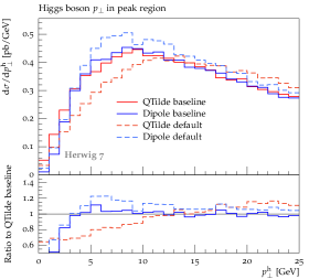
Figure 1: The Higgs boson transverse momentum spectrum comparing the two shower algorithms QTilde (red) and Dipole (blue) at their adjusted baseline settings used in this comparison.

To be more precise, we use a two-loop running, $\overline{\text{MS}}$, $\alpha_{s}$ including CMW correction Catani:1990rr with $\alpha_{s}^{CMW}(M_{Z})=0.126$ (which corresponds to $\alpha_{s}^{\overline{\text{MS}}}(M_{Z})=0.118$), and the MMHT2014 NLO PDF set Harland-Lang:2014zoa with five active flavours, interfaced through LHAPDF 6 Buckley:2014ana , as far as initial state radiation is concerned. Hard processes are simulated at leading order (see the previous discussion), using the Matchbox infrastructure powered by amplitudes generated by MadGraph5_aMC@NLO Alwall:2014hca . In $e^{+}e^{-}$ collissions, we consider di-jet production; at hadron colliders, in addition, we consider stable $Z$-boson Drell-Yan production, $(e^{+}e^{-}j)$ production within the mass window $66~{}\rm{GeV}<m_{ll}<116~{}\rm{GeV}$ around the $Z$ mass, as well as production of a stable, $125\ {\rm GeV}$, Higgs accompanied by zero or one jet. In the presence of additional jets in the hard process we use FastJet Cacciari:2006sm ; Cacciari:2011ma to perform the generation cuts; analyses are performed throughout using the Rivet framework Buckley:2010ar , with analysis modules based on existing experimental and generic Monte Carlo implementations. In $e^{+}e^{-}$ collisions, where we choose a centre of mass energy of $\sqrt{s}=100$ GeV as baseline, we reconstruct jets with the Durham algorithm Catani:1991hj , while the hadron collider setup reconstructs anti-$k_{\perp}$ jets with a radius of $R=0.4$ within a rapidity range $|y|<5$ and a transverse momentum threshold of $p_{\perp}>20\ {\rm GeV}$. Parton level without multiple interactions and hadronisation is employed, and partons up to and including $b$-quarks are treated as massless objects. Both parton showers mentioned above use a $p_{\perp}$ cutoff prescription with a value of $\mu_{\text{IR}}=1\ {\rm GeV}$. Electroweak parameters are kept at their default values.

2.5 Consistency Checks

The ability to compare different algorithms puts us into the unique position of performing a number of consistency checks for the uncertainty estimate that we advocate. In particular, perturbative error bands should cover algorithmic discrepancies, if these algorithms are expected to deliver the same accuracy. If that is not the case then the algorithm at hand is questionable. Furthermore, by construction the shower approximates emissions in the soft and collinear region. If we force the shower to produce hard emissions, larger uncertainties are to be expected by a controllable prescription. Another point is the possibility of double counting hard emissions. The shower should not cover phase-space regions that are already covered by the hard process input. This property is typically reflected in demanding that observables that receive input at fixed order are not significantly altered by subsequent showering. Clearly, the definition of ‘region’, which in this case is covered by the veto scale on hard emissions (see Sec. 3 for a more detailed discussion), is again only precise to the level of accuracy covered by the parton shower and varying this boundary should serve as a measure of missing logarithmic orders. We emphasise that a boundary chosen to be far away from the correct ordering behaviour may introduce severe double counting issues, ultimately impacting on a resummation of a tower of logarithms which is not typical to the process, i.e. not encountered in any higher order corrections to an observable considered. Furthermore, the perturbative uncertainties for observables in phase-space regions that do not receive logarithmically enhanced contributions should be driven by the hard scale alone, while the other scales have negligible impact. Logarithmically sensitive observables, on the other hand, should be altered by the parton shower and the uncertainties should be driven by all possible scale variations together. The setting where this is least clear is pure jet production, which we will address amongst other ‘jetty’ processes in Sec. 5.

3 Scale Choices, Variations and Profiles

3.1 Phase-Space Restrictions and Profile Choices

The quantity central to parton showers is the splitting kernel. Its exponentiation gives rise to the Sudakov form factor, which regulates the divergence of the splitting kernel for soft and/or collinear emissions. On top of this, there are two further crucial ingredients (besides formally subleading, though not necessarily small issues like kinematic parametrisations): The evolution variable chosen, and the phase space accessible at a fixed value of the evolution variable. Emissions are typically further subject to an upper bound on their hardness. This cannot be directly deduced from a priori principles but should be chosen in the order of magnitude of the typical hardness scale of the process being evolved to avoid the double counting issues mentioned before.

The central point we are concerned with in this section shall be summarised in a simplified model of final state radiation. Quite generally, we have to consider three different scales: a hard scale $K_{\perp}$ defining the phase space available to emissions at a fixed transverse momentum; a veto scale $Q_{\perp}$ defining the maximum transverse momentum available to emissions; and the kinematic limit of transverse momentum, $R_{\perp}$. We consider the $p_{\perp}$ spectrum of a single soft emission with splitting kernel (possibly after an appropriate transformation of the evolution variable into a transverse momentum)

$$P_{K_{\perp}^{2}}(p^{2}_{\perp},z)=C_{i}\frac{\alpha_{s}(p^{2}_{\perp})}{\pi}\frac{1}{1-z}\ \times\\ \theta(z_{+}(p^{2}_{\perp},K^{2}_{\perp})-z)\theta(z-z_{-}(p^{2}_{\perp},K^{2}_{\perp}))\ ,$$ (1)

where $C_{i}$ is the colour factor associated with the emitting leg. The longitudinal momentum fraction, $z$, has limits that read

$$z_{\pm}(p^{2}_{\perp},K^{2}_{\perp})=\frac{1}{2}\left(1\pm\sqrt{1-\frac{p_{\perp}^{2}}{K_{\perp}^{2}}}\right)\ ,$$ (2)

in the presence of a hard scale $K_{\perp}^{2}$. With emissions weighted by $\kappa$, an arbitrary function of a veto scale $Q_{\perp}^{2}$, we find a $p_{\perp}$ spectrum of the form

$$\frac{{\rm d}{\cal P}}{{\rm d}p_{\perp}^{2}{\rm d}z}=P_{K_{\perp}^{2}}(p^{2}_{\perp},z)\frac{\kappa(Q_{\perp}^{2},p_{\perp}^{2})}{p_{\perp}^{2}}\ \times\\ \theta(R_{\perp}^{2}-p_{\perp}^{2})\theta(p_{\perp}^{2}-\mu_{IR}^{2})\Delta_{K_{\perp}^{2}}(p_{\perp}^{2}|Q_{\perp}^{2})\ ,$$ (3)

with the Sudakov form factor

$$-\ln\Delta_{K_{\perp}^{2}}(p_{\perp}^{2}|Q_{\perp}^{2})=\\ \int_{p_{\perp}^{2}}^{R_{\perp}^{2}}\frac{{\rm d}q_{\perp}^{2}}{q_{\perp}^{2}}\kappa(Q_{\perp}^{2},q_{\perp}^{2})\int{\rm d}zP_{K_{\perp}^{2}}(q^{2}_{\perp},z)\ .$$ (4)

$R_{\perp}$ denotes the scale that makes all of phase space available to emissions, while we denote the infrared cutoff by $\mu_{IR}^{2}$ (we have not shown the zero $p_{\perp}$, non-radiating event contribution). Once a hard cutoff $\kappa(Q_{\perp}^{2},p_{\perp}^{2})=\theta(Q_{\perp}^{2}-p_{\perp}^{2})$ is chosen, this setup is known to reproduce the right anomalous dimensions. It has to be applied to a full evolution in a hierarchy $Q_{\perp}^{2}\to q_{\perp}^{2}$ where $K_{\perp}^{2}=Q_{\perp}^{2}$ is chosen and the form of the $z$ boundaries being crucial to produce the correct logarithmic pattern Platzer:2009jq ; Hoche:2015sya . Instead, if one desires to make all of the phase space available to parton shower emissions, $K_{\perp}^{2}=R_{\perp}^{2}$ is chosen and no other than the kinematic constraint $p_{\perp}^{2}<R_{\perp}^{2}$ is in place.

We have here considered the freedom of ensuring suppression of such emissions by an arbitrary function $\kappa$. We call this weighting function a profile scale choice. One of the subjects of the present study is to identify sensible profile scale choices; we stress that such a choice is of algorithmic nature and not an intrinsic source of uncertainty. We will consider the following choices, depicted in Fig. 2:

• theta: $\kappa(Q_{\perp}^{2},q_{\perp}^{2})=\theta(Q_{\perp}^{2}-q_{\perp}^{2})$, which is expected to reproduce the correct tower of logarithms;

• resummation: $\kappa(Q_{\perp}^{2},q_{\perp}^{2})$ is one below $(1-2\rho)\ Q_{\perp}$, zero above $Q_{\perp}$, and quadratically interpolating in between. This profile is expected to reproduce the correct towers of logarithms, and switches off the resummation smoothly towards the hard region (currently we use $\rho=0.3$ ):

  $$\kappa(Q_{\perp}^{2},q_{\perp}^{2})=\\ \left\{\begin{array}[]{ll}1&q_{\perp}/Q_{\perp}\leq 1-2\rho\\ 1-\frac{(1-2\rho-q_{\perp}/Q_{\perp})^{2}}{2\rho^{2}}&q_{\perp}/Q_{\perp}\in(1-2\rho,1-\rho]\\ \frac{(1-q_{\perp}/Q_{\perp})^{2}}{2\rho^{2}}&q_{\perp}/Q_{\perp}\in(1-\rho,1]\\ 0&q_{\perp}/Q_{\perp}>1\end{array}\right.\ ;$$ (5)

• hfact: $\kappa(Q_{\perp}^{2},q_{\perp}^{2})=\left(1+q_{\perp}^{2}/Q_{\perp}^{2}\right)^{-1}$, which is also referred to as damping factor within the POWHEG-BOX implementation Alioli:2010xd ; and

• power shower: imposing nothing but the phase-space restrictions inherent to the shower algorithm considered.

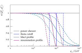
Figure 2: The different profile scale shapes considered in this study at a veto scale of $Q_{\perp}=100\ {\rm GeV}$ (solid) and $Q_{\perp}=50,200\ {\rm GeV}$ (dashed).

Different combinations of $R_{\perp}^{2}$ and $K_{\perp}^{2}$ can be achieved within the two showers. In particular, the dipole shower is able to populate the region up to $K_{\perp}^{2}=R_{\perp}^{2}$ (‘power shower’), while, for $2\to 1$ processes at hadron colliders the angular-ordered phase space, by construction, imposes $K_{\perp}^{2}=Q_{\perp}^{2}$ to be the mass of the singlet which is produced.

The leading logarithmic contribution of the $z$ integration at this simple qualitative level is given by

$$\int{\rm d}zP_{K_{\perp}^{2}}(q_{\perp}^{2},z)\sim\frac{C_{i}\alpha_{s}(q_{\perp}^{2})}{\pi}\log\left(\frac{K_{\perp}^{2}}{q_{\perp}^{2}}\right)\ .$$ (6)

We shall illustrate the impact of the profile scale choice $\kappa$ on the Sudakov form factor by considering a fixed $\alpha_{s}$, and evaluate

$$- \int_{p_{\perp}^{2}}^{R_{\perp}^{2}}\frac{{\rm d}q_{\perp}^{2}}{q_{\perp}^{2}}\kappa(Q_{\perp}^{2},q_{\perp}^{2})\log\left(\frac{K_{\perp}^{2}}{q_{\perp}^{2}}\right)=$$

$$- \frac{1}{2}\log^{2}\left(\frac{K_{\perp}^{2}}{p_{\perp}^{2}}\right)\kappa(Q_{\perp}^{2},p_{\perp}^{2})$$

$$+ \frac{1}{2}\log^{2}\left(\frac{K_{\perp}^{2}}{R_{\perp}^{2}}\right)\kappa(Q_{\perp}^{2},R_{\perp}^{2})$$

$$+ \frac{1}{2}\int_{p_{\perp}^{2}}^{R_{\perp}^{2}}{\rm d}q_{\perp}^{2}\log^{2}\left(\frac{K_{\perp}^{2}}{q_{\perp}^{2}}\right)\frac{\partial}{\partial q_{\perp}^{2}}\kappa(Q_{\perp}^{2},q_{\perp}^{2})\ .$$

To obtain the desired resummation properties, namely

$$\int_{p_{\perp}^{2}}^{R_{\perp}^{2}}\frac{{\rm d}q_{\perp}^{2}}{q_{\perp}^{2}}\kappa(Q_{\perp}^{2},q_{\perp}^{2})\log\left(\frac{K_{\perp}^{2}}{q_{\perp}^{2}}\right)\sim\frac{1}{2}\log^{2}\left(\frac{Q_{\perp}^{2}}{p_{\perp}^{2}}\right)\ ,$$ (8)

a number of limitations on $\kappa$ and the other scale choices need to be imposed. Clearly, the limiting cases for small and large transverse momenta need to be reproduced;

$$\kappa(Q_{\perp}^{2},p_{\perp}^{2})\to 1 p_{\perp}^{2}\ll Q_{\perp}^{2}\ ,$$ (9)

$$\kappa(Q_{\perp}^{2},p_{\perp}^{2})\to 0 q_{\perp}^{2}\sim R_{\perp}^{2}\gg Q_{\perp}^{2}\ .$$

While this is the case for all of the profiles we considered in this study, it is not sufficient to produce the desired tower of logarithms. Imposing the former restriction we still require that:

• $K_{\perp}^{2}\sim Q_{\perp}^{2}$ is imposed by the $z$ boundaries; and

• $\kappa(Q_{\perp}^{2},q_{\perp}^{2})\sim\text{const}$ whenever $q_{\perp}^{2}$ is not of the order of $Q_{\perp}^{2}$ for the term involving the derivative of $\kappa$ to become subleading.

Specifically the first restriction is only guaranteed by either the angular-ordered phase space which naturally imposes this restriction, or the restricted phase space chosen for the dipole shower. The second restriction also excludes choices of $\kappa$ providing a ratio of logarithms to effectively replace $K_{\perp}^{2}$ by $Q_{\perp}^{2}$ in the first term in Eq. 3.1. To this extent, we conclude that only those profiles that are narrow smeared versions (in the sense of varying only in a region where $Q_{\perp}^{2}/q_{\perp}^{2}$ is of order one) of a theta-type cutoff will provide the proper tower of logarithms. Choices such as the resummation profile are desirable to avoid discontinuities introduced by the theta-type cutoff which are beyond the accuracy considered, while keeping the resummation properties of the parton shower; the profile we consider here is only one such kind, and there is no restriction on the exact form considered. The name ‘profile’ is chosen since the treatment of the hard scale we consider here closely resembles prescriptions on scale variations within the analytic resummation context Tackmann:Profiles .

3.2 Identifying a ‘Resummation Scale’

The hard veto scale $Q_{\perp}^{2}$ is the scale that, when considering transverse momentum spectra as outlined in the previous section, is closest in role to a resummation scale in analytical resummation. However, it is not typically the same as a shower starting scale. Though in our case this statement is true for the dipole shower, no such notion exists for the angular-ordered shower where typically the masses of the emitting dipoles set the shower starting scale owing to the angular-ordered phase space. In the latter case, emissions exceeding the transverse momenta of jets present in the hard process are possible and an additional veto on transverse momenta generated by the shower is applied; the value of this veto is, in this case, the analogue of the starting scale of the dipole shower. The resummation scale of the typical $q_{\perp}$-resummation can thus not directly be related to an analogue hard scale present in different shower algorithms, especially when they evolve in a variable different from the transverse momentum and hence built up the full spectrum from multiple, differently ordered emissions.

For both the showers considered here, transverse momenta of parton shower emissions are expected to be limited or suppressed by the scale $Q_{\perp}^{2}$, which on very general grounds should thus be of the order of a typical scale of the hard process, i.e. the factorisation scale. As with fixed-order calculations the residual dependence on $Q_{\perp}^{2}$ is expected to become smaller as more and more logarithmic orders are incorporated. This implies a pattern of scale compensation through successive logarithmic orders, which a parton shower can typically only guarantee at the level of at most next-to-leading logarithms (NLL).

3.3 Scale Variations

Having chosen a reasonable profile scale and value of $K_{\perp}^{2}\sim Q_{\perp}^{2}$, the leading behaviour of the Sudakov exponent takes the well-known form

$$-\ln\Delta(p_{\perp}^{2}|Q_{\perp}^{2})=\\ \int_{p_{\perp}^{2}}^{Q_{\perp}^{2}}\frac{{\rm d}q^{2}}{q^{2}}\left(A(\alpha_{s}(q^{2}))\ln\left(\frac{Q_{\perp}^{2}}{q^{2}}\right)+B(\alpha_{s}(q^{2}))\right)\ ,$$ (10)

where the highest level of accuracy one can hope for with coherent evolution is NLL accuracy, neglecting subleading colour correlations, at least for some observables and typically limited phase-space regions Catani:1990rr ,

$$A(\alpha_{s})=\frac{C_{i}}{2}\frac{\alpha_{s}}{\pi}\left(1+\frac{K_{g}}{2}\frac{\alpha_{s}}{\pi}\right)\qquad B(\alpha_{s})=\frac{\alpha_{s}}{\pi}\frac{\gamma_{i}}{2}$$ (11)

along with a two-loop running of $\alpha_{s}$.

In addition to variations of the scales in the hard process, $\mu^{\prime}_{R/F}=\xi_{H}\mu_{R/F}$, we vary both the hard veto scale, $\mu_{Q}=\xi_{Q}Q_{\perp}$, and the arguments of $\alpha_{s}$ and the PDFs in the parton shower splitting kernels, $\mu_{S}=\xi_{S}q_{\perp}$. We constrain the number of possible variations to be $\xi\in[1/2,1,2]$. This spans a cube of, $\xi_{H}\otimes\xi_{S}\otimes\xi_{Q}$, 27 combinations. All these choices are connected to logarithmic scale choices. There is therefore no a priori way of reducing their number. We emphasise that in principle only the full 27-point envelope constitutes a comprehensive uncertainty measure. We therefore always produce the full envelope along with envelopes for each of the individual variations. Using this it is possible to observe which scale drives the overall uncertainty in a particular region of phase space. While one clearly expects the variation of $Q_{\perp}^{2}$ to cancel out to the level of NLL accuracy Hamilton:Scales (if this is indeed resembled by the parton shower), the situation is less clear for the other variation and different proposals have been made as to what extent the contribution at the level of NLL contributions should be canceled (see e.g. Dasgupta:2001eq for a discussion) or otherwise considered as a probe of where precisely higher accuracy of the shower is missing. We do not consider introducing any terms that cancel these variations to the NLL order, and postpone a detailed analysis of this issue to future work. We do, however, analyse these variations as we are convinced that they are another clean handle on controlling where we expect, specifically, soft emissions and contributions by the hadronisation model to dominate. A recent Les Houches study LesHouches:2015 has also shown that, when not taking into account the full variations of this kind, discrepancies between different shower algorithms, which are expected to be similar, are not covered within these variations.

3.4 Real-life Constraints

Besides the unclear definition of a resummation scale in the context of different shower algorithms, another word of caution needs to be raised when considering the hard veto scales: There are cases in which there is no meaningful variation as the hard scale is a fixed quantity such as the mass of an independently evolving final state emitting system, e.g. showers in $e^{+}e^{-}\to$ hadrons. It is not clear how one would quantify the respective shower uncertainty in this case, besides looking at shape differences encountered at different centre-of-mass energies of the $e^{+}e^{-}$ collider to quantify the scaling of the predictions with respect to ratios of the hard scale to the infrared sensitive quantity considered. Already this observation clearly marks the fact that no claim of a full and well-understood uncertainty recipe can be made at this point, but only are we able to perform initial steps in this direction. Similarly for the power shower there is no meaningful variation of $\mu_{Q}$. It can also happen, as is the case for the angular-ordered shower, that the algorithm chosen naturally imposes an upper bound on the hardness of the emission. In the case of Drell-Yan type processes, the angular-ordered shower, for example, will only allow for a down-variation of $Q_{\perp}^{2}$ and is thus questionable as to whether this variation in these cases is the right measure.

As with the small scales probed in the evolution of the parton shower, $\mu_{R,F}$ variations in the shower may actually encounter regions where typically some cutoff or freezing-like behaviour is imposed to both, the running of $\alpha_{s}$ and the parton distributions functions, which may result in interesting dynamics when variation of such small scales is used to infer uncertainties – a variation of the freezing prescription may thus be desirable, as well.

4 Clean Benchmarks

To begin exploring the uncertainties that arise from the considerations of Sec. 3 we start by studying ‘clean benchmarks’, i.e. hard processes with the least number of legs: $e^{+}e^{-}$ annihilation, and Drell-Yan-type $2\to 1$ processes producing either a $Z$ or Higgs boson. For the case of $e^{+}e^{-}$ collisions, the notion of a hard veto scale does not directly exist owing to the fact that the phase-space boundary and relevant hard scale coincide. However, we can compare variations of the collision energy and quantify this impact at the level of normalised distributions to acquire a handle on variations of the logarithmic structure similar to hadron-hadron collisions. On top of the three scales $\mu_{H,S,Q}$ described above, we vary the infrared cutoff of the shower by a factor of $1/2$ and $2$ for the $e^{+}e^{-}$ setting, in order to obtain a first indication of how much dynamics of the shower is expected to be absorbed into hadronisation effects; notice that varying the argument of $\alpha_{s}$ may serve a similar purpose.

4.1 Final State Showers

$e^{+}e^{-}\to qq$ provides the clean environment to study final state radiation. Note that in this case the power and theta profile coincide, which is also our choice in the following.

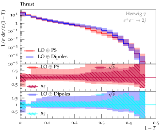
Figure 3: Thrust distribution for the QTilde shower (red) and Dipole shower (blue). The main plot envelopes consist of the variations $\sqrt{s}\otimes\mu_{S}$. The ratio plot for each individual shower contains the contributions from the individual variation of each scale which are shown relative to the full envelope (ratio, top-left).

The Thrust distribution, Fig. 3, shows good agreement between showers; this is true both for the central prediction and its variations, and shows that they possess the same resummation accuracy. Differences that do emerge between the showers are related to cutoff effects and non-radiating events in the region towards $T=1$; these offer no insight into the resummation properties. A further difference emerges from the dead-zone of the QTilde shower, however this is a region that can be supplemented by using matching or ME corrections. For this observable we note that the $\sqrt{s}$ and $\mu_{S}$ variations are similar in magnitude.

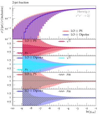
Figure 4: Distribution of the 2-jet fraction against $y_{\mathrm{cut}}$. The main plot contains the envelope of the scale variations $\sqrt{s}\otimes\mu_{S}$ for the QTilde shower (red) and Dipole shower (blue). The first two ratio plots contain the contributions from the individual variation of each scale relative to the full envelope (ratio, top-left). The last two ratio plots show the $\mu_{\mathrm{IR}}$ variations (ratio, top-right), and, for size comparison, we also plot the envelopes of the main plot (ratio, top-left).

In Fig. 4 we show results for the integrated two-jet rate; the uncertainties are dominated by $\sqrt{s}$ as well as cutoff variations at small $y_{\mathrm{cut}}$. Again, the overall uncertainties are comparable between the showers; as expected, we obtain large uncertainties in the small $y_{\rm cut}$ region, which is dominated by hadronisation effects.

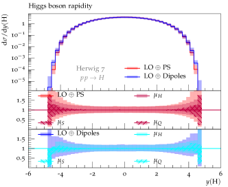
Figure 5: Rapidity of the Higgs boson for both the QTilde shower (red) and the Dipole shower (blue). The main plot envelope contains the full scale variations for each shower, and the ratio plots contain their breakdown in terms of the individual scales relative to the full envelope (ratio, top-left). The lines shown are for the resummation profile.

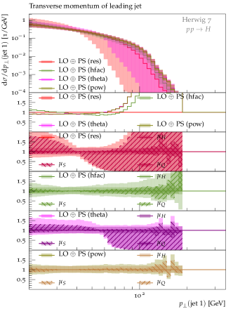
Figure 6: Transverse momentum of the leading jet in Higgs production with the QTilde shower. The main plot envelopes consist of the full set of $\mu_{H},\mu_{S},\mu_{Q}$ variations for the resummation (red), hfact (green), theta (pink), pow (brown). The first ratio plot shows the central predictions for each profile relative to the resummation profile. The subsequent ratio plots show the variations of individual scales relative to the full envelope for each profile (ratio, top-left).

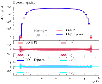
Figure 7: Rapidity of the Z boson for both the QTilde shower (red) and the Dipole shower (blue). The main plot envelope contains the full scale variations for each shower, and the ratio plots contain their breakdown in terms of the individual scales relative to the full envelope (ratio, top-left). The lines shown are for the resummation profile.

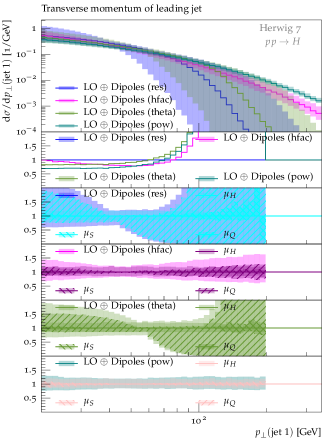
Figure 8: Transverse momentum of the leading jet in Higgs production with the Dipole shower. The main plot envelopes consist of the full set of $\mu_{H},\mu_{S},\mu_{Q}$ variations for the resummation (blue), hfact (pink), theta (green), pow (teal). The first ratio plot shows the central predictions for each profile relative to the resummation profile. The subsequent ratio plots show the variations of individual scales relative to the full envelope for each profile (ratio, top-left).

4.2 Initial State Showers

As far as initial-state showering is concerned, we investigate a gluon-initiated process $pp\to H$ (in the large-$m_{t}$ effective theory), and a quark-initiated process $pp\to Z$; these particles are set stable for simplicity. Inclusive observables, such as the rapidity of the resonance in this case, are quantities expected to be well described by the matrix element, and thus should be unmodified by the parton shower; this is reflected in Figs. 5 and 7 where both showers display good agreement, with uncertainties mainly driven by the hard process variation. The differences in magnitude should be attributed to different couplings for each process, with envelope shape differences attributed to the PDFs.

The jets in these samples are generated solely from the parton shower; therefore the $p_{\perp}$ of the leading (hardest) jet directly probes the impact of the profile scales.

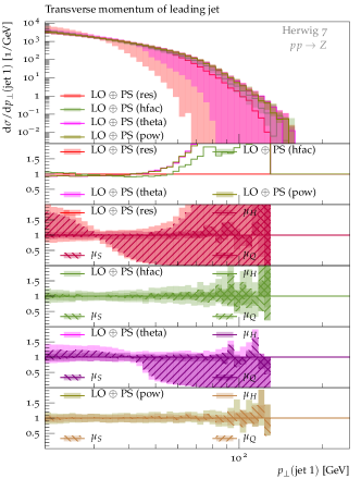
Figure 9: Transverse momentum of the leading jet in Z production with the QTilde shower. The main plot envelopes consist of the full set of $\mu_{H},\mu_{S},\mu_{Q}$ variations for the resummation (red), hfact (green), theta (pink), pow (brown). The first ratio plot shows the central predictions for each profile relative to the resummation profile. The subsequent ratio plots show the variations of individual scales relative to the full envelope for each profile (ratio, top-left).

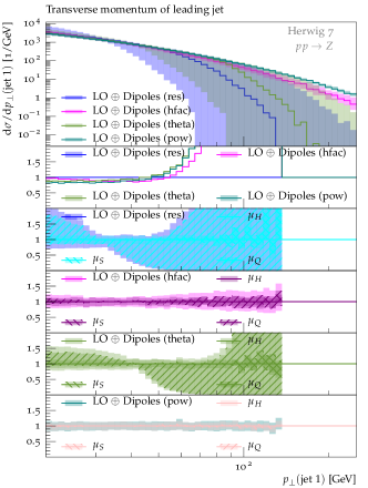
Figure 10: Transverse momentum of the leading jet in Z production with the Dipole shower. The main plot envelopes consist of the full set of $\mu_{H},\mu_{S},\mu_{Q}$ variations for the resummation (blue), hfact (pink), theta (green), pow (teal). The first ratio plot shows the central predictions for each profile relative to the resummation profile. The subsequent ratio plots show the variations of individual scales relative to the full envelope for each profile (ratio, top-left).

Comparing Figs. 6-10, we find that the different profile choices exhibit significantly different behaviours, both amongst themselves as well as between different showers. The resummation and theta profiles, as intended, yield comparable results in terms of central predictions and uncertainties and across the different shower algorithms. This clearly shows that we can indeed expect the same resummation accuracy using these profiles. The variations towards high $p_{\perp}$ for the theta profile expose the effect of the different phase-space limitations. In the QTilde shower the upward variation of the scales ($\mu_{Q}$) is ultimately irrelevant, as there are no possible emissions at this scale; looking at the dipole shower one sees the effect of such variations. However, this is not the case for the resummation profile whose interpolating region is sensitive to such variations, and displays similar variations between showers.

For large transverse momenta, the uncertainties should reflect the case that parton-shower emissions in these regions are unreliable. We observe this for both the theta and resummation profiles and to some extent for the hfact choice, though the variation is considerably smaller than indicated by the theta-type choices. The power shower, however, shows no increased uncertainty and in fact is dominated by variations of $\mu_{H}$. Given the marked differences in the hardness of jets between the two showers, the power shower seems to offer no handle towards the assessment of shower uncertainties. We can also clearly observe the intrinsic limitation of the QTilde shower phase space, that in this case is not able to populate high-$p_{\perp}$ emissions which ultimately needs to be supplied by matching and/or matrix element corrections similarly to the ‘dead zone’ effect in $e^{+}e^{-}$ collisions.

We therefore conclude that within this basic setting the showers and profile scale choices do admit the expected behaviour, and the two showers using theta-type profiles exhibit similar central predictions and uncertainties.

5 Jetty Processes

Having established shower uncertainties using simple benchmark processes, the next simplest examples are the processes studied in Sec. 4 with an additional hard emission off the hard process, e.g. $H/Z$ plus one (inclusive) jet. In addition, pure di-jet production is investigated because of the absence of a colour singlet setting a hard scale and the related ambiguities in possible hard scale choices. We do not investigate the shower cutoff as we shall now focus on properties which are not expected to be significantly altered by hadronisation effects.

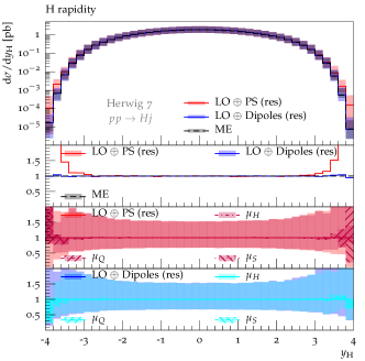
Figure 11: Rapidity of the Higgs in Higgs plus one jet events for the QTilde (red) and Dipole (blue) shower compared to the matrix element prediction (black). We show results obtained with the resummation profile. The error bands are computed from all allowed scale choices (see text). Top ratio plot: QTilde vs. Dipole and ME. Second ratio plot: QTilde with full error band vs. variation of only either $\mu_{H}$, $\mu_{Q}$ or $\mu_{S}$. Third ratio plot: Dipole with full error band vs. variation of only either $\mu_{H}$, $\mu_{Q}$ or $\mu_{S}$.

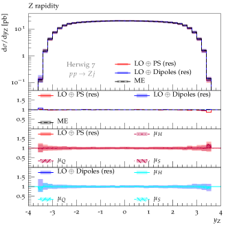
Figure 12: Rapidity of the Z in Z plus one jet events for the QTilde (red) and Dipole (blue) shower compared to the matrix element prediction (black). We show results obtained with the resummation profile. The error bands are computed from all allowed scale choices (see text). Top ratio plot: QTilde vs. Dipole and ME. Second ratio plot: QTilde with full error band vs. variation of only either $\mu_{H}$, $\mu_{Q}$ or $\mu_{S}$. Third ratio plot: Dipole with full error band vs. variation of only either $\mu_{H}$, $\mu_{Q}$ or $\mu_{S}$.

As with the clean benchmarks presented in Sec. 4, we consider variations of the three relevant scales discussed in Sec. 3, changing them by factors $1/2$ and $2$, respectively, to span a cube of a total of $27$ variations; we will also perform cross-validations between both available showers. From arguments given in Sec. 3 we expect observables and/or regions in phase space where the uncertainty is mainly driven by $\xi_{\text{H}}$, i.e. in the case of inclusive observables. As all uncertainties connected with scale choices stem from logarithmic arguments there is no a priori way to exclude any of the possible variations when determining shower uncertainties, unless one is able to identify scale compensation patterns between the different scales for which we see no evidence in the setting considered in this study.

For the rapidity distributions of the Higgs and $Z$ boson, shown in Fig. 11 and 12, respectively, we find that the distributions are consistent with the prediction of the hard matrix element, as is expected from such inclusive quantities; this applies to all of the profile scales considered, with the power shower showing larger deviations in the forward region. Scale variations affect these observable mainly through variations present in the hard process.

Similarly to the rapidity distributions, we expect the $p_{\perp}$-spectra of the leading jet to be predicted mainly by the hard matrix element, according to the consistency conditions discussed in Sec. 2.5. In Fig. 13 and 14 (H and Z production, respectively) we show the results for the QTilde shower, while Fig. 15 and 16 contain our findings for the Dipole shower. We again find that the uncertainties are dominated by the variation of the hard scale. For both showers the resummation profile is consistent with the hard matrix element prediction, except for jets close to the threshold where cut migration effects are being probed. For the hfact profile with the QTilde shower we find a spectrum compatible with the one anticipated by the matrix element; for the dipole shower, a significantly harder spectrum is obtained. A similar, but even more dramatic picture emerges for the power shower setting. The spread of predictions for the QTilde shower is smaller than the spread for the dipole shower, owing to the intrinsic limitations of the phase-space volume available to angular-ordered emissions as already pointed out in the previous sections. The combinations QTilde plus power, and Dipole plus hfact or power contradict the criterion of controllable showering, which in this case is expected to not significantly alter the jet $p_{\perp}$ spectrum. Combined with the empirical findings of Sec. 4, we will therefore not consider the power shower profile choice any further.

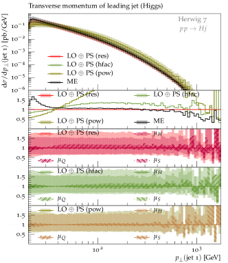
Figure 13: Transverse momentum of the leading jet for Higgs plus one (inclusive) jet as computed by the QTilde shower for resummation (red), hfact (lime) and power (brown) profile compared to the ME (black) prediction. Top ratio plot: same as before. Other ratio plots: resummation, hfact respectively power profile with full error band vs. variation of only either $\mu_{H}$, $\mu_{Q}$ or $\mu_{S}$.

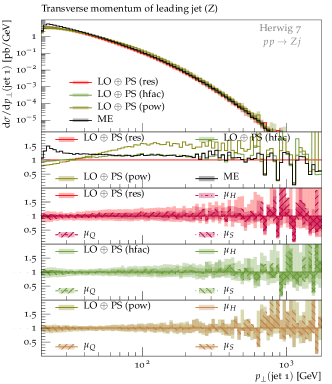
Figure 14: Transverse momentum of the leading jet for Z plus one (inclusive) jet as computed by the QTilde shower for resummation (red), hfact (lime) and power (brown) profile compared to the ME (black) prediction. Top ratio plot: same as before. Other ratio plots: resummation, hfact respectively power profile with full error band vs. variation of only either $\mu_{H}$, $\mu_{Q}$ or $\mu_{S}$.

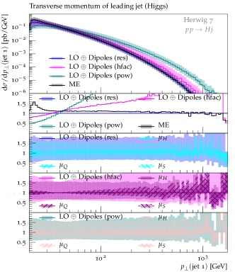
Figure 15: Transverse momentum of the leading jet for Higgs plus one (inclusive) jet as computed by the Dipole shower for resummation (red), hfact (lime) and power (brown) profile compared to the ME (black) prediction. Top ratio plot: same as before. Other ratio plots: resummation, hfact respectively power profile with full error band vs. variation of only either $\mu_{H}$, $\mu_{Q}$ or $\mu_{S}$.

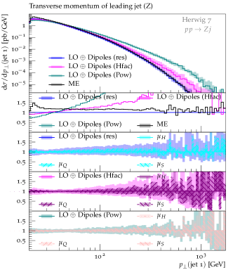
Figure 16: Transverse momentum of the leading jet for Z plus one (inclusive) jet as computed by the Dipole shower for resummation (red), hfact (lime) and power (brown) profile compared to the ME (black) prediction. Top ratio plot: same as before. Other ratio plots: resummation, hfact respectively power profile with full error band vs. variation of only either $\mu_{H}$, $\mu_{Q}$ or $\mu_{S}$.

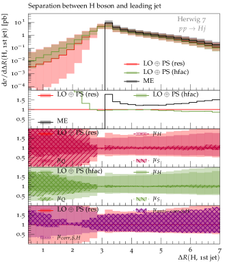
Figure 17: Separation between the Higgs and the leading jet for Higgs plus one (inclusive) jet as computed by the QTilde shower for resummation (red) and hfact (lime) profile compared to the ME (black) prediction. Top ratio plot: same as before. Second and third ratio plots: resummation respectively hfact profile with full error band vs. variation of only either $\mu_{H}$, $\mu_{Q}$ or $\mu_{S}$. Last ratio plot: resummation profile with full error band vs a subset where $\mu_{H}$ and $\mu_{S}$ are varied in correlated (dark purple) respectively anti-correlated (hatched) manner, while $\mu_{Q}$ is held fixed.

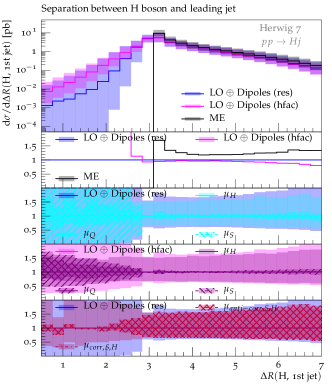
Figure 18: Separation between the Higgs and the leading jet for Higgs plus one (inclusive) jet as computed by the Dipole shower for resummation (red) and hfact (lime) profile compared to the ME (black) prediction. Top ratio plot: same as before. Second and third ratio plots: resummation respectively hfact profile with full error band vs. variation of only either $\mu_{H}$, $\mu_{Q}$ or $\mu_{S}$. Last ratio plot: resummation profile with full error band vs. a subset where $\mu_{H}$ and $\mu_{S}$ are varied in a correlated (dark purple) respectively anti-correlated (hatched) manner, while $\mu_{Q}$ is held fixed.

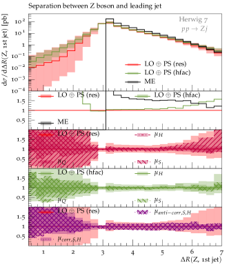
Figure 19: Separation between the Z and the leading jet for Z plus one (inclusive) jet as computed by the QTilde shower for resummation (red) and hfact (lime) profile compared to the ME (black) prediction. Top ratio plot: same as before. Second and third ratio plots: resummation respectively hfact profile with full error band vs. variation of only either $\mu_{H}$, $\mu_{Q}$ or $\mu_{S}$. Last ratio plot: resummation profile with full error band vs a subset where $\mu_{H}$ and $\mu_{S}$ are varied in a correlated (dark purple) respectively anti-correlated (hatched) manner, while $\mu_{Q}$ is held fixed.

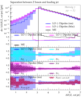
Figure 20: Separation between the Z and the leading jet for Z plus one (inclusive) jet as computed by the Dipole shower for resummation (red) and hfact (lime) profile compared to the ME (black) prediction. Top ratio plot: same as before. Second and third ratio plots: resummation respectively hfact profile with full error band vs. variation of only either $\mu_{H}$, $\mu_{Q}$ or $\mu_{S}$. Last ratio plot: resummation profile with full error band vs a subset where $\mu_{H}$ and $\mu_{S}$ are varied in a correlated (dark purple) respectively anti-correlated (hatched) manner, while $\mu_{Q}$ is held fixed.

Turning to more exclusive observables, we consider the angular separation between the boson and the leading jet $\Delta R_{(H/Z)j}$, which probes both matrix element and shower dominated regions in a continuous observable: Matrix element emissions in this case can only populate the phase-space region $\Delta R_{(H/Z)j}\geq\pi$. The region below is solely filled by the parton shower, typically operating at the boundary of validity of the underlying approximation as this phase space requires the shower to produce a hard, large-angle emission. Within the definition of controllable and consistent uncertainties, we therefore expect large uncertainties for $\Delta R_{(H/Z)j}\leq\pi$, while the shower should reproduce the matrix element dynamics above. Results for the QTilde shower are shown in Fig. 17 and 19 (H and $Z$ production, respectively) and for the Dipole shower in Fig. 18 and 20. We place particular emphasis on the comparison of the resummation and hfact profiles. For all processes/showers we find that hfact predicts a small uncertainty band and produces slightly more hard jets; the latter can be attributed to the available phase space, while the former can be obtained by analysing Eq. 3.1, stressing the fact that the region in which the derivative of the profile is varying significantly extends over a larger region than for the other profiles, though with less overall variation implied. Contrary, and matching the expectations motivated by the logarithmic structure, the uncertainty for the resummation profile in the small $\Delta R_{(H/Z)j}$ region is large and driven by all scale variations together. In addition, in the bottom ratio plot of Figs. 17, 19, 18 and 20 we show a subset of scale variations for the resummation profile choice, varying the hard and shower scales in a correlated and anti-correlated setting, at a fixed $\mu_{Q}$. This breakdown shows how different subsets of variations constitute the full uncertainty band. Besides the simple domination of the uncertainty by one variation, other regions of phase space show that the uncertainty is strongly underestimated by considering the variations separately. We therefore argue that only the full, combined, scale variation produces a reliable error band.

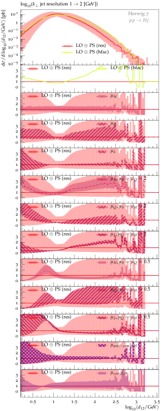
Figure 21: $k_{\perp}$–splitting scale for the transition from the one to the two jet configuration in Higgs plus one (inclusive) jet as computed with the QTilde shower. The base line in each plot is the resummation profile choice. The main plot and the first ratio plot show a comparison to the hfact profile choice. The subsequent ratio plots compare the full error band to certain subsets of scale variation choices, namely: variation of $\mu_{H}$, $\mu_{Q}$, $\mu_{S}$, $\mu_{H}$ with $\xi_{Q}$ and $\xi_{S}$ fixed to 2, $\mu_{Q}$ with $\xi_{H}$ and $\xi_{S}$ fixed to 2, $\mu_{S}$ with $\xi_{Q}$ and $\xi_{H}$ fixed to 2, $\mu_{H}$ with $\xi_{Q}$ and $\xi_{S}$ fixed to 0.5, $\mu_{Q}$ with $\xi_{H}$ and $\xi_{S}$ fixed to 0.5, $\mu_{S}$ with $\xi_{Q}$ and $\xi_{H}$ fixed to 0.5, $\mu_{S}$ and $\mu_{H}$ in a correlated manner and $\mu_{S}$ and $\mu_{H}$ in an anti-correlated manner.

As another probe of the interaction of shower emissions with the hardest jet, we consider $k_{\perp}$-splitting scales, particularly the one in which an event with two jets would turn into an event with one jet as the jet $p_{\perp}$ threshold passes through the scale obtained. These observables have also been proven to be accessible to analytic considerations Gerwick:2014koa , for which comparisons to full parton showers are highly desirable though are beyond the scope of this paper. In Fig. 21 we show our results for the QTilde shower for Higgs production. Once again we compare the resummation profile choice with the hfact profile. It is noteworthy that the hfact profile introduces a strong change in the shape of the Sudakov peak, on top of the harder spectrum already observed for the first jet; besides the tail effects we are therefore concerned that profile scale choices along these lines may significantly impact the resummation properties of the parton shower, as may already be expected from the arguments presented in Sec. 3. We therefore conclude that, even with intrinsically restricted phase space, the hfact profile does not provide controllable uncertainties and will not be taken further into account in this study. We also use Fig. 21 to perform an comprehensive breakdown of the different variation directions in the ‘cube’ of possible variations, showing that no individual variation actually covers the full dynamics present. For LO plus PS simulations, we therefore argue that the full band is taken into consideration and improvements in the context of matching and merging will be subject to future work.

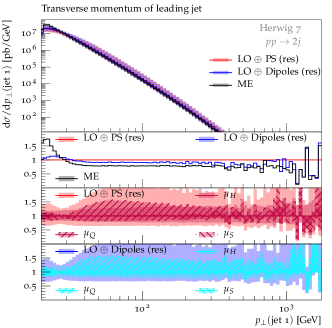
Figure 22: Transverse momentum of the first jet in (inclusive) di-jet production as computed by the QTilde (red) and Dipole (blue) shower with the resummation profile compared to the ME (black) prediction. Top ratio plot: same as before. Subsequent ratio plots: QTilde (second) and Dipole (third) with full error band vs. variation of only either $\mu_{H}$, $\mu_{Q}$ or $\mu_{S}$.

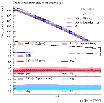
Figure 23: Transverse momentum of the second jet in (inclusive) di-jet production as computed by the QTilde (red) and Dipole (blue) shower with the resummation profile compared to the ME (black) prediction. Top ratio plot: same as before. Subsequent ratio plots: QTilde (second) and Dipole (third) with full error band vs. variation of only either $\mu_{H}$, $\mu_{Q}$ or $\mu_{S}$.

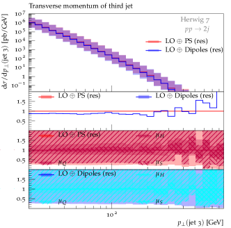
Figure 24: Transverse momentum of the third jet (inclusive) di-jet production as computed by the QTilde (red) and Dipole (blue) shower with the resummation profile compared to the ME (black) prediction. Top ratio plot: same as before. Other ratio plots: QTilde (second) and Dipole (third) with full error band vs. variation of only either $\mu_{H}$, $\mu_{Q}$ or $\mu_{S}$.

We have so far considered processes with a colourless, massive object that dominates the scale hierarchy at hand, and, even in the presence of an additional jet, makes the dynamics rather insensitive to additional radiation (as far as this radiation is confined to reasonable phase-space regions as identified above). A process where this is clearly not the case is pure jet production in hadron collisions, which also probes different colour structures that have not been encountered in the hard processes considered thus far. Owing to the back-to-back configuration at lowest order, we expect considerable parton-shower effects in comparison to the hard matrix element for a number of observables and expect to make a more detailed comparison to fixed order only once NLO improvement has been incorporated. Nevertheless, we can still test as to what extent the shower variations match up to expectations in signalling regions where the prediction should generally be considered unreliable. We also test, once more, if the two showers are comparable within their uncertainties. Following the previous arguments, we only consider the resummation profile, with a hard scale again given by the jet $p_{\perp}$. Sample results comparing to the hard matrix element are shown in Figs. 22, 23 and 25, which show that the two showers preform in a very similar way both in their central predictions and variations; they also show that qualitatively we find a behaviour similar to the singlet plus jet benchmarks as if we had replaced the hard, colourless, object with a jet as hard probe. Quantitatively, however, we observe significant changes in rates for the second jet, which need to be confronted with the impact of cut migration as well as the impact of higher order corrections. We also note that choosing the hard veto scale in this setting has a significant impact on showered results.

With the transverse momentum of the third jet and the $2\to 3$ resolution shown in Figs. 24 and 26 we consider purely shower driven quantities; both of these nicely reveal that the two showers, together with the resummation profile, are perfectly compatible with each other, exhibiting the same resummation accuracy.

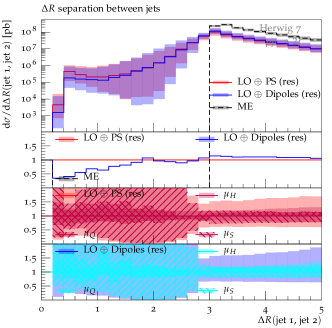
Figure 25: Separation between the leading and second jet for (inclusive) di-jet as computed by the QTilde (red) and the Dipole (blue) shower together with the resummation profile. Top ratio plot: same as before. Second and third ratio plots: full error band vs. variation of only either $\mu_{H}$, $\mu_{Q}$ or $\mu_{S}$.

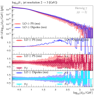
Figure 26: $k_{\perp}$–splitting scale for the transition from the two to the three jet configuration in (inclusive) di-jet production as computed with the QTilde (red) and the Dipole (blue) shower together with the resummation profile. The base line in the first plot is the QTilde shower. The subsequent ratio plots compare the full error band to certain subsets of scale variation choices, namely: variation of $\mu_{H}$, $\mu_{Q}$, $\mu_{S}$. The second ratio plot presents the QTilde shower, the last one the Dipole shower.

6 Conclusions and Outlook

We have performed a comprehensive and detailed study of the sources of uncertainty in parton showers, utilising the two parton-shower algorithms available in Herwig 7. We have investigated different choices of profile scales to approach the boundary of hard emissions, as these are highly relevant to effects that appear in the context of NLO plus PS matching. We have systematically categorised the sources of uncertainty and outlined their interplay with other simulation components, putting this study into context of a bigger work programme to eventually establish uncertainties for event generators in total.

Focussing on the perturbative, parton-shower part, of the simulation, we have deliberately chosen LO plus PS calculations to establish a baseline of controllable and consistent variations that will allow us to subsequently identify improvements and reduction in these uncertainties as higher order corrections are included. We have found that profile scale choices are very constrained when applying consistency conditions on both central predictions (which should not alter input distributions of the hard process) and uncertainties (with large uncertainties to be expected in unreliable regions or regions dominated by hadronisation corrections), as well as stable results in the Sudakov region. Particularly the hfact and power shower configurations do not admit results compatible with these criteria. Utilising a resummation profile, which is very close to the theta cutoff for hard emissions as implemented in previous algorithms, we find that the angular-ordered and dipole-based shower algorithms are compatible with each other, both in central predictions and uncertainty claims, despite their very different nature.

References

- (1) M. Bahr et al., Herwig++ Physics and Manual, Eur. Phys. J. C58 (2008) 639–707, [arXiv:0803.0883].
- (2) J. Bellm et al., Herwig 7.0/Herwig++ 3.0 release note, Eur. Phys. J. C76 (2016), no. 4 196, [arXiv:1512.0117].
- (3) T. Sjöstrand, S. Mrenna, and P. Skands, Pythia 6.4 physics and manual, Journal of High Energy Physics 2006 (2006), no. 05 026.
- (4) T. Sjöstrand, S. Ask, J. R. Christiansen, R. Corke, N. Desai, P. Ilten, S. Mrenna, S. Prestel, C. O. Rasmussen, and P. Z. Skands, An Introduction to PYTHIA 8.2, Comput. Phys. Commun. 191 (2015) 159–177, [arXiv:1410.3012].
- (5) T. Sjostrand, S. Mrenna, and P. Z. Skands, A Brief Introduction to PYTHIA 8.1, Comput. Phys. Commun. 178 (2008) 852–867, [arXiv:0710.3820].
- (6) T. Gleisberg, S. Hoeche, F. Krauss, M. Schonherr, S. Schumann, F. Siegert, and J. Winter, Event generation with SHERPA 1.1, JHEP 02 (2009) 007, [arXiv:0811.4622].
- (7) S. Alioli, P. Nason, C. Oleari, and E. Re, A general framework for implementing NLO calculations in shower Monte Carlo programs: the POWHEG BOX, JHEP 06 (2010) 043, [arXiv:1002.2581].
- (8) S. Plätzer and S. Gieseke, Dipole Showers and Automated NLO Matching in Herwig++, Eur. Phys. J. C72 (2012) 2187, [arXiv:1109.6256].
- (9) S. Hoeche, F. Krauss, M. Schonherr, and F. Siegert, A critical appraisal of NLO+PS matching methods, JHEP 09 (2012) 049, [arXiv:1111.1220].
- (10) A. J. Larkoski, J. J. Lopez-Villarejo, and P. Skands, Helicity-Dependent Showers and Matching with VINCIA, Phys. Rev. D87 (2013), no. 5 054033, [arXiv:1301.0933].
- (11) J. Alwall et al., The automated computation of tree-level and next-to-leading order differential cross sections, and their matching to parton shower simulations, JHEP 07 (2014) 079, [arXiv:1405.0301].
- (12) K. Hamilton, P. Nason, E. Re, and G. Zanderighi, NNLOPS simulation of Higgs boson production, JHEP 10 (2013) 222, [arXiv:1309.0017].
- (13) S. Höche, Y. Li, and S. Prestel, Drell-Yan lepton pair production at NNLO QCD with parton showers, Phys. Rev. D91 (2015), no. 7 074015, [arXiv:1405.3607].
- (14) M. Czakon, H. B. Hartanto, M. Kraus, and M. Worek, Matching the Nagy-Soper parton shower at next-to-leading order, JHEP 06 (2015) 033, [arXiv:1502.0092].
- (15) S. Jadach, W. Płaczek, S. Sapeta, A. Siódmok, and M. Skrzypek, Matching NLO QCD with parton shower in Monte Carlo scheme — the KrkNLO method, JHEP 10 (2015) 052, [arXiv:1503.0684].
- (16) S. Hoeche, F. Krauss, M. Schonherr, and F. Siegert, QCD matrix elements + parton showers: The NLO case, JHEP 04 (2013) 027, [arXiv:1207.5030].
- (17) R. Frederix and S. Frixione, Merging meets matching in MC@NLO, JHEP 12 (2012) 061, [arXiv:1209.6215].
- (18) S. Alioli, C. W. Bauer, C. J. Berggren, A. Hornig, F. J. Tackmann, C. K. Vermilion, J. R. Walsh, and S. Zuberi, Combining Higher-Order Resummation with Multiple NLO Calculations and Parton Showers in GENEVA, JHEP 09 (2013) 120, [arXiv:1211.7049].
- (19) L. Lonnblad and S. Prestel, Unitarising Matrix Element + Parton Shower merging, JHEP 02 (2013) 094, [arXiv:1211.4827].
- (20) S. Plätzer, Controlling inclusive cross sections in parton shower + matrix element merging, JHEP 08 (2013) 114, [arXiv:1211.5467].
- (21) L. Lönnblad and S. Prestel, Merging Multi-leg NLO Matrix Elements with Parton Showers, JHEP 03 (2013) 166, [arXiv:1211.7278].
- (22) R. Frederix and K. Hamilton, Extending the MINLO method, arXiv:1512.0266.
- (23) S. Platzer and M. Sjodahl, Subleading improved Parton Showers, JHEP 07 (2012) 042, [arXiv:1201.0260].
- (24) Z. Nagy and D. E. Soper, Effects of subleading color in a parton shower, JHEP 07 (2015) 119, [arXiv:1501.0077].
- (25) S. Höche and S. Prestel, The midpoint between dipole and parton showers, Eur. Phys. J. C75 (2015), no. 9 461, [arXiv:1506.0505].
- (26) N. Fischer and P. Skands, Coherent Showers for the LHC, 2016. arXiv:1604.0480.
- (27) C. Bierlich, G. Gustafson, L. Lönnblad, and A. Tarasov, Effects of Overlapping Strings in pp Collisions, JHEP 03 (2015) 148, [arXiv:1412.6259].
- (28) J. R. Christiansen and P. Z. Skands, String Formation Beyond Leading Colour, JHEP 08 (2015) 003, [arXiv:1505.0168].
- (29) Particle Data Group Collaboration, K. A. Olive et al., Review of Particle Physics, Chin. Phys. C38 (2014) 090001.
- (30) P. M. Stevenson, Resolution of the Renormalization Scheme Ambiguity in Perturbative QCD, Phys. Lett. B100 (1981) 61.
- (31) S. J. Brodsky, G. P. Lepage, and P. B. Mackenzie, On the elimination of scale ambiguities in perturbative quantum chromodynamics, Phys. Rev. D 28 (Jul, 1983) 228–235.
- (32) I. W. Stewart and F. J. Tackmann, Theory Uncertainties for Higgs and Other Searches Using Jet Bins, Phys. Rev. D85 (2012) 034011, [arXiv:1107.2117].
- (33) M. Cacciari and N. Houdeau, Meaningful characterisation of perturbative theoretical uncertainties, JHEP 09 (2011) 039, [arXiv:1105.5152].
- (34) A. David and G. Passarino, How well can we guess theoretical uncertainties?, Physics Letters B 726 (2013), no. 1–3 266 – 272.
- (35) E. Bagnaschi, M. Cacciari, A. Guffanti, and L. Jenniches, An extensive survey of the estimation of uncertainties from missing higher orders in perturbative calculations, JHEP 02 (2015) 133, [arXiv:1409.5036].
- (36) G. Bozzi, S. Catani, D. de Florian, and M. Grazzini, Transverse-momentum resummation and the spectrum of the Higgs boson at the LHC, Nucl. Phys. B737 (2006) 73–120, [hep-ph/0508068].
- (37) C. F. Berger, C. Marcantonini, I. W. Stewart, F. J. Tackmann, and W. J. Waalewijn, Higgs Production with a Central Jet Veto at NNLL+NNLO, JHEP 04 (2011) 092, [arXiv:1012.4480].
- (38) ATLAS Collaboration, G. Aad et al., Luminosity public results run2, 2016.
- (39) CMS Collaboration, V. Khachatryan et al., Public CMS luminosity information, 2016.
- (40) C. Englert, T. Plehn, P. Schichtel, and S. Schumann, Jets plus Missing Energy with an Autofocus, Phys. Rev. D83 (2011) 095009, [arXiv:1102.4615].
- (41) C. Englert, T. Plehn, P. Schichtel, and S. Schumann, Establishing Jet Scaling Patterns with a Photon, JHEP 02 (2012) 030, [arXiv:1108.5473].
- (42) P. Richardson and D. Winn, Investigation of Monte Carlo Uncertainties on Higgs Boson searches using Jet Substructure, Eur. Phys. J. C72 (2012) 2178, [arXiv:1207.0380].
- (43) M. H. Seymour and A. Siodmok, Constraining MPI models using and recent Tevatron and LHC Underlying Event data, JHEP 10 (2013) 113, [arXiv:1307.5015].
- (44) M. H. Seymour and C. Tevlin, A Comparison of two different jet algorithms for the top mass reconstruction at the LHC, JHEP 11 (2006) 052, [hep-ph/0609100].
- (45) S. Plätzer and S. Gieseke, Coherent Parton Showers with Local Recoils, JHEP 01 (2011) 024, [arXiv:0909.5593].
- (46) S. Hoeche, F. Krauss, and M. Schonherr, Uncertainties in MEPS@NLO calculations of h+jets, Phys. Rev. D90 (2014), no. 1 014012, [arXiv:1401.7971].
- (47) D. Bourilkov, Study of parton density function uncertainties with LHAPDF and PYTHIA at LHC, in LHC / LC Study Group Meeting Geneva, Switzerland, May 9, 2003, 2003. hep-ph/0305126.
- (48) S. Gieseke, Uncertainties of Sudakov form-factors, JHEP 01 (2005) 058, [hep-ph/0412342].
- (49) A. Buckley, Sensitivities to PDFs in parton shower MC generator reweighting and tuning, arXiv:1601.0422.
- (50) S. Hoeche and M. Schonherr, Uncertainties in next-to-leading order plus parton shower matched simulations of inclusive jet and dijet production, Phys. Rev. D86 (2012) 094042, [arXiv:1208.2815].
- (51) N. E. Adam, V. Halyo, and S. A. Yost, Evaluation of the theoretical uncertainties in the cross sections at the lhc, Journal of High Energy Physics 2008 (2008), no. 05 062.
- (52) M. W. Krasny, F. Fayette, W. Placzek, and A. Siodmok, Z-boson as ’the standard candle’ for high precision W-boson physics at LHC, Eur. Phys. J. C51 (2007) 607–617, [hep-ph/0702251].
- (53) F. Fayette, M. W. Krasny, W. Placzek, and A. Siodmok, Measurement of at LHC, Eur. Phys. J. C63 (2009) 33–56, [arXiv:0812.2571].
- (54) M. W. Krasny, F. Dydak, F. Fayette, W. Placzek, and A. Siodmok, at the LHC: a forlorn hope?, Eur. Phys. J. C69 (2010) 379–397, [arXiv:1004.2597].
- (55) K. Cranmer, S. Kreiss, D. Lopez-Val, and T. Plehn, Decoupling Theoretical Uncertainties from Measurements of the Higgs Boson, Phys. Rev. D91 (2015), no. 5 054032, [arXiv:1401.0080].
- (56) P. Bartalini, R. Chierici, and A. de Roeck, Guidelines for the Estimation of Theoretical Uncertainties at the LHC, Tech. Rep. CMS-NOTE-2005-013, CERN, Geneva, Sep, 2005.
- (57) P. Stephens and A. van Hameren, Propagation of uncertainty in a parton shower, hep-ph/0703240.
- (58) S. Gieseke, P. Stephens, and B. Webber, New formalism for QCD parton showers, JHEP 12 (2003) 045, [hep-ph/0310083].
- (59) M. Bahr, S. Gieseke, and M. H. Seymour, Simulation of multiple partonic interactions in Herwig++, JHEP 07 (2008) 076, [arXiv:0803.3633].
- (60) M. Bahr, J. M. Butterworth, and M. H. Seymour, The Underlying Event and the Total Cross Section from Tevatron to the LHC, JHEP 01 (2009) 065, [arXiv:0806.2949].
- (61) S. Gieseke, C. Rohr, and A. Siodmok, Colour reconnections in Herwig++, Eur. Phys. J. C72 (2012) 2225, [arXiv:1206.0041].
- (62) M. Bengtsson and T. Sjostrand, A Comparative Study of Coherent and Noncoherent Parton Shower Evolution, Nucl. Phys. B289 (1987) 810.
- (63) T. Sjostrand, A Model for Initial State Parton Showers, Phys. Lett. B157 (1985) 321.
- (64) S. Catani, B. R. Webber, and G. Marchesini, QCD coherent branching and semiinclusive processes at large x, Nucl. Phys. B349 (1991) 635–654.
- (65) L. A. Harland-Lang, A. D. Martin, P. Motylinski, and R. S. Thorne, Parton distributions in the LHC era: MMHT 2014 PDFs, Eur. Phys. J. C75 (2015) 204, [arXiv:1412.3989].
- (66) A. Buckley et al., LHAPDF6: parton density access in the LHC precision era, Eur. Phys. J. C75 (2015) 132, [arXiv:1412.7420].
- (67) M. Cacciari, FastJet: A Code for fast k(t) clustering, and more, hep-ph/0607071.
- (68) M. Cacciari, G. P. Salam, and G. Soyez, FastJet User Manual, Eur. Phys. J. C72 (2012) 1896, [arXiv:1111.6097].
- (69) A. Buckley et al., Rivet user manual, Comput. Phys. Commun. 184 (2013) 2803–2819, [arXiv:1003.0694].
- (70) S. Catani, Y. L. Dokshitzer, M. Olsson, G. Turnock, and B. R. Webber, New clustering algorithm for multi - jet cross-sections in e+ e- annihilation, Phys. Lett. B269 (1991) 432–438.
- (71) F. Tackmann, Private communication.
- (72) K. Hamilton, Private communication.
- (73) M. Dasgupta and G. P. Salam, Resummation of the jet broadening in DIS, Eur. Phys. J. C24 (2002) 213–236, [hep-ph/0110213].
- (74) S. Hoeche, A. Jueid, G. Nail, S. Plätzer, et al., Towards parton shower variations, To appear in: Proceedings of the 2015 Les Houches workshop.
- (75) E. Gerwick and P. Schichtel, Jet properties at high-multiplicity, arXiv:1412.1806.