Testing the cosmic conservation of photon number with type Ia supernovae and ages of old objects

Abstract

In this paper, we obtain luminosity distances by using ages of 32 old passive galaxies distributed over the redshift interval $0.11<z<1.84$ and test the cosmic conservation of photon number by comparing them with 580 distance moduli of type Ia supernovae (SNe Ia) from the so-called Union 2.1 compilation. Our analyses are based on the fact that the method of obtaining ages of galaxies relies on the detailed shape of galaxy spectra but not on galaxy luminosity. Possible departures from cosmic conservation of photon number is parametrized by $\tau(z)=2\epsilon z$ and $\tau(z)=\epsilon z/(1+z)$ (for $\epsilon=0$ the conservation of photon number is recovered). We find $\epsilon=0.016^{+0.078}_{-0.075}$ from the first parametrization and $\epsilon=-0.18^{+0.25}_{-0.24}$ from the second parametrization, both limits at 95% c.l. In this way, no significant departure from cosmic conservation of photon number is verified. In addition, by considering the total age as inferred from Planck (2015) analysis, we find the incubation time $t_{inc}=1.66\pm 0.29$ Gyr and $t_{inc}=1.23\pm 0.27$ Gyr at 68% c.l. for each parametrization, respectively.

I Introduction

Since 1998, type Ia supernovae (SNe Ia) observations (Riess et al. 1998, Perlmutter et al. 1998, Suzuki et al. 2012, Bertoule et al. 2014) have been an important tool to access the current cosmic acceleration and test different cosmological models. In order to explain cosmic acceleration, if one wants to preserve Einstein’s General Relativity Equations together with spacetime isotropy and homogeneity, one has to postulate some source of negative pressure. The sources of negative pressure that have been hypothesized include Einstein’s cosmological constant (Padmanabhan 2003; Frieman, Turner & Huterer 2008; Weinberg 2013), dark energy (Lima 2004; Caldwell & Kamionkowski 2009; Li et al. 2011; Frieman, Turner & Huterer 2008; Weinberg 2013) and quantum matter creation from gravitational field (Lima et al. 2008; Steigman et al. 2009; Lima et al. 2010; Graef et al. 2014; Jesus & Andrade-Oliveira 2016).

However, this important evidence arising from SNe Ia observations has been questioned through the years and some alternative explanations to the observations have been given. Examples are possible evolutionary effects in SNe Ia events (Drell, Loredo & Wasserman 2000; Combes 2004), local Hubble bubble (Zehavi et al. 1998; Conley et al. 2007), modified gravity (Ishak, Upadhye & Spergel 2006; Kunz & Sapone 2007; Bertschinger & Zukin 2008), unclustered sources of light attenuation (Aguirre 1999; Rowan-Robinson 2002; Goobar, Bergstrom & Mortsell 2002) and the existence of Axion-Like-Particles (ALPs), arising in a wide range of well-motivated high-energy physics scenarios, and that could lead to the dimming of SNe Ia brightness (Avgoustidis et al. 2009, 2010). Nowadays, the dark energy is supported by several independent observational data, such as baryon acoustic oscillations (BAO) and other galaxy clusters observations, cosmic background radiation, observational Hubble constant data as well as age of the Universe (see Frieman, Turner & Huterer 2008 and Weinberg 2013). Besides an accelerated stage, the high $z$ observational data also indicate a decelerated phase for $z>1$, fundamental for the structure formation process to take place (Riess et al. 2004).

With more than 700 Type Ia supernovae discovered (Betoule et al. 2014), the constraints on cosmological parameters inferred from SNe Ia are now limited by systematic errors rather than by statistical errors. An important systematic error source is the mapping of the cosmic opacity. The SNe Ia observations are affected by at least four different sources of opacity, namely, the Milky Way, the hosting galaxy, intervening galaxies, and the Intergalactic Medium. The opacity can also occur by extragalactic magnetic fields that can turn photons into unobserved particles (e.g. light axions, chameleons, gravitons, Kaluza-Klein modes) (Avgoustidis et al. 2009 & 2010). Recently, an interesting result was obtained by Lima, Cunha & Zanchin (2011). These authors discussed two different scenarios with cosmic absorption and concluded that only if the cosmic opacity is fully negligible, the description of an accelerating Universe powered by dark energy or some alternative gravity theory must be invoked (see also Li et al. 2013).

An interesting way to test the quality of the SNe Ia data has been performed in recent years by confronting them with data sets which are cosmic opacity independent. For instance, Holanda, Carvalho & Alcaniz (2013) as well as Liao, Avgoustidis & Zhengxiang (2015) used current measurements of the expansion rate $H(z)$ and SNe Ia data to impose cosmological model-independent constraints on cosmic opacity. These authors found that a completely transparent universe is in agreement with the data considered (see also Avgoustidis et al. 2009, 2010 for analyses in a flat $\Lambda$CDM framework). Holanda & Busti (2014) explored the possible existence of an opacity at higher redshifts ($z>2$) in $\Lambda$CDM context by using $H(z)$ data and luminosity distance of gamma ray bursts. The samples were compatible with a transparent universe at 1$\sigma$ level. Chen et al. (2012) by using baryons acoustic oscillations (BAO) (Eisenstein et al. 2005) and SN Ia data found that an opaque universe is preferred in redshift regions $0.20-0.35$, $0.35-0.44$ and $0.60-0.73$, whereas a transparent universe is favoured in redshift regions $0.106-0.20$, $0.44-0.57$ and $0.57-0.60$. When these authors considered the entire redshift range, their result were still consistent with a transparent universe at $1\sigma$ confidence level (c.l.). By testing the luminosity distance of SNe Ia with ADD from galaxy clusters, Li et al. (2013) have put constraints on cosmic opacity. However, the limits thus obtained rely on the assumptions used to describe the galaxy clusters morphology. The results of Holanda, Carvalho & Alcaniz (2013) also rely on the SNe Ia light curve fitter (SALT2, MLCS2K2). In this way, it is still interesting to investigate and compare different observational data and look for any systematics in them.

On the other hand, other interesting results have arisen from this kind of analysis, with an excessive brightness being also detected in SNe Ia data. In this context, Nair, Jhingan & Deepak (2012) compared distance measurements obtained from SNe Ia and BAO and they found that the supernovae are brighter than expected from BAO measurements. Obtaining a similar result, Basset & Kunz (2004) found a $2\sigma$ violation caused by excess brightening of SNe Ia at $z>0.5$ when confronted them via cosmic distance duality relation with angular diameter distances (ADD) from compact objects, perhaps due to lensing magnification bias. However, such result also may come from some exotic sources of photon involving a coupling of photons to particles beyond the standard model of particle physics. An interesting effect occurs if there is mixing between photons and chameleons (a scalar particle which arises in certain models of scalar-tensor gravity) in presence of a strong magnetic field. In this context, observers on Earth see a brightened image of the SNe Ia (see Burrage 2008 and Avgoustidis et al. 2010).

In this paper, we show that it is possible to test the cosmic conservation of photon number with luminosity distances from SNe Ia and those inferred from 32 ages of old objects. We do not assume any matter content in our analysis. Our analyses are based on the fact that the method of obtaining ages of galaxies relies on the detailed shape of galaxy spectra but not on galaxy luminosity. Moreover, it is only assumed that the Universe is homogeneous and isotropic, which leads to the Friedmann-Robertson-Walker geometry (see Eq. 3). As a simplifying hypothesis, we assume spatial flatness. In addition to the present analysis, in order to put constraints over $t_{inc}$, we use the Planck constraint on the cosmic total age (Ade et al. 2016). As a result, no significant departure from cosmic conservation of photon number is verified.

The paper is organized as follows. In Section II we describe our new method to verify the photon conservation, while in Section III the observational quantities used in this work are discussed. The corresponding constraints on the opacity are investigated and discussed in Section IV. We summarize our main results in Section V.

II Methodology

II.1 Photon conservation and luminosity distances

As well known, a violation of photon number from a luminosity source leads to a modification of its inferred luminosity distance, increasing or decreasing it with respect to a transparent universe. Mathematically, if there is violation of photon number between observer and a light source, the flux received is modified by a factor $e^{-\tau(z)}$, where $\tau>0$ corresponds to a photon sink and $\tau<0$ corresponds to a photon source in the path to the observer (Chen & Kantowski, 2009a; 2009b). In this way, the inferred luminosity distance of the source, $D_{L,obs}$ is related to the true luminosity distance (in a transparent universe) by

$$D^{2}_{L,obs}=D^{2}_{L,true}e^{\tau(z)}.$$ (1)

Therefore, the observed distance modulus is given by

$$m_{obs}=m_{true}+2.5[\log e]\tau(z).$$ (2)

In our analyses, measurements of $m_{obs}$ are taken from the SNe Ia Union 2.1 compilation (Suzuki et al. 2012). We compare $m_{obs}$ estimates from SNe Ia data to $m_{true}$ inferred directly from the ages of old objects as will be discussed in the next subsection.

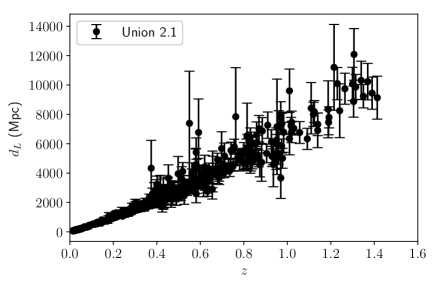
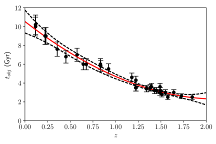
Figure 1: (a) Luminosity distances of SNe Ia from Union 2.1 compilation. (b) $t_{obj}(z)$ corresponding to the estimated ages of the galaxies. The solid red and dashed black lines are the best fit and 2$\sigma$ error, respectively, obtained from a fit by using a third degree polynomial.

II.2 Luminosity distance from old objects

Let us assume the Friedmann-Robertson-Walker metric and that the method of obtaining ages of galaxies relies on the detailed shape of galaxy spectra but not on galaxy luminosity. Thus, the true luminosity distance can be obtained from ages of old objects as follows (Jimenez & Loeb 2002)

$$D_{L,true}=(1+z)c\int_{z}^{0}\left[(1+z)\frac{dt}{dz}\right]dz,$$ (3)

where $t$ is the Universe age at redshift $z$. In this way, if one can access the $dt/dz$ quantity in SNe Ia redshift range without assumptions on cosmological model and also free of opacity, it is possible to obtain $m_{true}$ for each SNe Ia redshift and put constraints on $\tau(z)$ via Eq. (2).

In our work, $dt/dz$ is estimated from ages of 32 old passive galaxies distributed over the redshift interval $0.11<z<1.84$ (see next section for details). In Fig. 1b we plot the original estimated ages of galaxies (see next section for more details). As we are only interested on the derivative $dt/dz$, instead of assuming an incubation time and using the total age from other observations, we choose to fit $t_{obj}(z)$. If we assume that the incubation time is constant, that is, independent of redshift, one may see that $t(z)$ only differs from $t_{obj}(z)$ by a constant. That is,

$$t(z)=t_{obj}(z)+t_{inc}.$$ (4)

We have tested some polynomial fits for $t_{obj}(z)$ and we have found that the minimal polynomial that yields a good fit, when combined with SNe Ia, is a third degree polynomial fit, such as:

$$t_{obj}(z)=a_{0}+a_{1}z+a_{2}z^{2}+a_{3}z^{3}.$$ (5)

As we assume $t_{inc}$ to be constant, we have $\frac{dt_{obj}}{dz}=\frac{dt}{dz}$, so we may say, that our model of Universe, that is, the function we assume that can describe the Universe given the data is:

$$\frac{dt}{dz}=a_{1}+2a_{2}z+3a_{3}z^{2}$$ (6)

From (4), we may also estimate $t_{inc}$, once we estimate $a_{0}$ and know $t_{0}$, as we have $t_{inc}=t_{0}-a_{0}$. Finally, from Eq. (3), the true luminosity distance can be given by

$$D_{L}(z)=c(1+z)\left[-a_{1}\left(z+\frac{z^{2}}{2}\right)-a_{2}\left(z^{2}+\frac{2z^{3}}{3}\right)-a_{3}\left(z^{3}+3\frac{z^{4}}{4}\right)\right].$$ (7)

However, one must note that the parameters $a_{i}$ derived from the age of old objects will be in Gyr, so in order to obtain $D_{L}$ in Mpc in Eq. (7) one must write $c$ in Mpc/Gyr as $c=306.6$ Mpc/Gyr.

III Data set

In the following, we describe the data sets used in our analyses.

• For the photon number dependent data, we use the Union 2.1 SNe Ia sample. This sample is an update of the original Union compilation (Amanullah et al. 2010) that comprises 580 data points including recent large samples from other surveys and uses SALT2 for SNe Ia lightcurve fitting (Guy et al. 2007). As the Union 2.1 consists of several subsamples, Suzuki et al. (2012) allowed a different absolute magnitude value for each subsample thereby making the impact of the cosmological model negligible. This sample is plotted in Fig. 1a, with the luminosity distances obtained via the known relation $D_{L}(z)=10^{(\mu(z)-25)/5}$, where $\mu$ is the distance modulus, and the corresponding $\sigma_{D_{L}}=\frac{dD_{L}}{d\mu}\sigma_{\mu}$.

• For the photon number independent data, we use the age estimates of 32 old passive galaxies distributed over the redshift interval $0.11<z<1.84$, as recently analysed by Simon, Verde & Jimenez (2005) (see Fig. 1b). The total sample is composed by three sub-samples: 10 field early-type galaxies from Treu et al. (1999, 2001, 2002), whose ages were obtained by using SPEED models of Jimenez et al. (2004); 20 red galaxies from the publicly released Gemini Deep Deep Survey (GDDS) whose integrated light is fully dominated by evolved stars (Abraham et al. 2004, McCarthy et al. 2004). Simon, Verde & Jimenez (2005) re-analysed the GDDS old sample by using a different stellar population models and obtained ages within 0.1 Gyr of the GDDS collaboration estimates - and the two radio galaxies LBDS 53W091 and LBDS 53W069 (Dunlop et al. 1996; Spinrad et al. 1997; Nolan et al. 2001).

  Recently, Wei et al. (2015) obtained $t_{inc}=1.36$ Gyr and $t_{inc}=1.62$ Gyr by considering this galaxy sample in a flat $\Lambda$CDM model with fixed and free $H_{0}$ (Hubble parameter) and $\Omega_{m}$ parameters, respectively. This factor accounts for our ignorance about the amount of time since the beginning of the structure formation in the Universe until the formation time of the object. However, such a treatment assumes that all of these galaxies need to have formed at the same time for their ages to trace out the Universe history. We still assume $10\%$ uncertainty on measurement of age of each Galaxy (Dantas et al. 2009, 2011; Samushia et al. 2010). Again, it is also important to stress that the method for obtaining the age of galaxies relies on the detailed shape of galaxy spectra but not on galaxy luminosity, so it is independent of $\tau$ (Avgoustidis et al. 2010).

IV Analyses and discussion

We assume two possible departures from cosmic conservation of photon number, as parametrized by two functions:

• P1: $\tau(z)=2\epsilon z$. This linear expression can be derived from the usual cosmic distance duality relation parametrization $D_{L}=D_{A}(1+z)^{2+\epsilon}$ for small values of $\epsilon$ and $z\leq 1$, where $\epsilon$ quantifies departures from cosmic conservation of photon number (see Avgoustidis et al. 2009).

• P2: $\tau(z)=\epsilon z/(1+z)$, which avoids the $\tau(z)$ divergence at high redshifts of the linear parametrization.

As one may see, $\epsilon>0$ and $\epsilon<0$ correspond, respectively, to the presence of a cosmic opacity or photon source between the observer and the light source.

We estimate the best-fit to the set of parameters ${\mathbf{p}}\equiv(\epsilon,a_{0},a_{1},a_{2},a_{3})$ through a joint analysis involving the luminosity distances of SNe Ia and age of galaxies by evaluating the likelihood distribution function, ${\cal{L}}\propto e^{-\chi^{2}/2}$, with

$$\chi^{2}(\mathbf{p}) = \chi^{2}_{tz}(a_{0},a_{1},a_{2},a_{3})+\chi^{2}_{SN}(\epsilon,a_{1},a_{2},a_{3})$$ (8)

where

$$\chi^{2}_{tz} = \sum_{i=1}^{32}\frac{(t_{obj,obs,i}-t_{obj}(z_{i},a_{0},a_{1},a_{2},a_{3}))^{2}}{\sigma^{2}_{t_{obj},obs,i}}$$ (9)

and

$$\chi^{2}_{SN} = \sum_{i=1}^{580}\frac{(m_{obs,i}-m_{true}(z_{i},a_{1},a_{2},a_{3})-1.085736\tau(z_{i},\varepsilon))^{2}}{\sigma^{2}_{m,obs,i}},$$ (10)

In Eq. (9), $t_{obj}(z_{i},a_{0},a_{1},a_{2},a_{3})$ is obtained from Eq.(5) and $t_{obj,obs,i}$ corresponds to ages of galaxies. In Eq. (10), $m_{true}(z_{i},a_{1},a_{2},a_{3})=5\log_{10}D_{L,true}+25$, with $D_{L,true}$ obtained from Eq. (7). The quantities $m_{obs,i}$ and $\sigma^{2}_{m,obs,i}$ are the distance modulus and their uncertainties from SNe Ia, respectively.

Because there is so many free parameters in both models, we choose to sample the likelihood through Monte Carlo Markov Chain (MCMC) analysis. A simple and powerful MCMC method is the so called Affine Invariant MCMC Ensemble Sampler by Goodman and Weare (2010), which was implemented in Python language with the emcee software by Foreman-Mackey et al. (2013). This MCMC method has the advantage over simple Metropolis-Hasting (MH) methods of depending on only one scale parameter of the proposal distribution and on the number of walkers. While MH methods in general depend on the parameter covariance matrix, that is, it depends on $n(n+1)/2$ tuning parameters, where $n$ is dimension of parameter space. The main idea of the Goodman-Weare affine-invariant sampler is the so called “stretch move”, where the position (parameter vector in parameter space) of a walker (chain) is determined by the position of the other walkers. Foreman-Mackey et al. modified this method, in order to make it suitable for parallelization, by splitting the walkers in two groups, then the position of a walker in one group is determined by only the position of walkers of the other group.

We used the freely available software emcee to sample from our likelihood in our 5-dimensional parameter space. We have used flat priors over the parameters. In order to plot all the constraints in the same figure, we have used the freely available software getdist, in its Python version. The results of our statistical analyses from Eq. (8) can be seen in Fig. 2 and Table 1, where the errors correspond to 68.3% and 95% c.l.

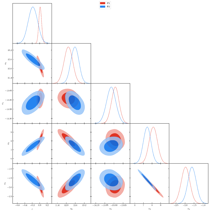
Figure 2: The results of our statistical analysis, with constraints from SNe Ia Union 2.1 data and ages of old objects. Diagonal: Likelihoods for the parameters on each indicated model, $P_{1}$ (red) and $P_{2}$ (blue). Below diagonal: Contours for 68.3% and 95.4% confidence intervals for each indicated model, $P_{1}$ and $P_{2}$. The $a_{i}$ parameters have units of Gyr. Although we represent the $\epsilon$ parameter of each model in the same column, they have different meanings, because they correspond to different $\tau_{i}(z)$.

From Fig. 2 and Table 1, we see that both functions (P1, P2) favour a cosmic conservation of photon number at least at 2$\sigma$ c.l. Figure 3a shows the marginalized likelihoods for $\epsilon$ in both models. An interesting result appears when the evolution of $\tau(z)$ is plotted. As one may see in Fig. 3b, the transparent universe, $\tau(z)=0$, is in full agreement with the data used in our analyses at 1$\sigma$ c.l. for model P1 and 2$\sigma$ c.l. for model P2.

Parameter	P1	P2
$\epsilon$	$0.016^{+0.078}_{-0.075}$	$-0.18^{+0.25}_{-0.24}$
$a_{0}$ (Gyr)	$12.14\pm 0.58$	$12.57^{+0.54}_{-0.53}$
$a_{1}$ (Gyr)	$-13.778^{+0.13}_{-0.13}$	$-13.845^{+0.15}_{-0.15}$
$a_{2}$ (Gyr)	$8.16^{+0.49+0.96}_{-0.48-0.96}$	$7.43^{+0.86}_{-0.87}$
$a_{3}$ (Gyr)	$-1.98^{+0.48}_{-0.47}$	$-1.61\pm 0.46$
$\chi^{2}_{red}$	$0.981$	$0.978$

Table 1: Marginalized results for the free parameters of models P1 and P2. The central values shown correspond to mean values of the parameters and the errors correspond to 95% c.l. The best fit values are much similar, as the distributions are quite symmetrical.

As one may see on Table 1, the parameter errors are quite small, corresponding to 2.4% (P1) and 2.1% (P2) over $a_{0}$ (68.3% c.l.), for example. This is due to the large number of SNe Ia and to the fact that the $t_{obj}(z)$ and SNe Ia are complementary, yielding nearly orthogonal constraints.

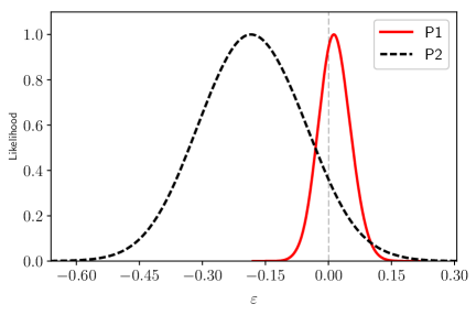
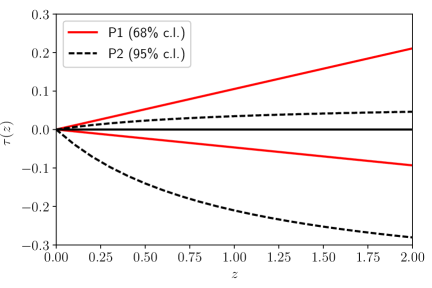
Figure 3: (a) Likelihood functions for $\epsilon$. (b) Confidence intervals on the plane $\tau-z$, 68% c.l. for P1 and 95% c.l. for P2. In both figures the solid and dashed lines correspond to results from P1 and P2.

As we have claimed before, we may estimate incubation time in context of our models once we have estimated $a_{0}$ and by taking the total age from Planck (Ade et al., 2016). The total age indicated by Ade et al. in their TT+lowP+lensing analysis, in the context of flat $\Lambda$CDM model, was $t_{0}=13.799\pm 0.038$ Gyr. As $t_{inc}=t_{0}-a_{0}$, we have $t_{inc}=1.66\pm 0.29$ Gyr for model P1 and $t_{inc}=1.23\pm 0.27$ Gyr for model P2, both at 68% c.l. These values are in agreement with the ones obtained by Wei et al. (2015), in the context of flat $\Lambda$CDM model, where they have found $t_{inc}=1.36$ Gyr for fixed and $t_{inc}=1.62$ Gyr for free $H_{0}$ and $\Omega_{m}$ parameters.

IV.1 Comparing results

At this point it is interesting to compare our results with previous ones that used the linear parametrization and different observations. For instance, Avgoustidis et al. (2009, 2010) via SNe Ia and $H(z)$ data obtained $\epsilon=-0.01^{+0.08}_{-0.09}$ and $\epsilon=-0.04^{+0.08}_{-0.07}$ in the flat $\Lambda$CDM framework. Holanda, Carvalho & Alcaniz (2013) by using only SNe Ia + $H(z)$ observations obtained $\epsilon=0.017\pm 0.055$. Holanda & Busti (2014) by using gamma ray bursts + $H(z)$ observations obtained $\epsilon=0.03\pm 0.10$ and $\epsilon=0.028\pm 0.10$ in flat $\Lambda$CDM and XCDM frameworks, respectively. More recently, Liao, Avgoustidis & Li (2015) also used only SNe Ia + $H(z)$ data, but they have taken into account the covariance between the distances from $H(z)$ measurements obtained from integration on the $H(z)$ data, found $\epsilon=0.07^{+0.11}_{-0.12}$, in full agreement with our results. None of these analyses have been able to discard a transparent Universe ($\epsilon=0$).

V Conclusions

In this paper we have proposed a new model cosmological independent method to probe the cosmic conservation of photon number. Although that the Universe acceleration for redshifts approximately lower than unity is supported by several other independent probes, investigating the cosmic opacity on the SNe Ia data is an important issue, in order to search for some source of unknown systematic error. If some extra dimming or brightness is still present, the SNe Ia observations will give us unreal values to main cosmological parameters and the Universe will seem as accelerating at a different rate than it actually is.

To perform our analyses, we have considered the following cosmological data: 580 SNe Ia from Union 2.1 compilation and old objects, specifically, 32 old galaxies ($0.11<z<1.84$). Since the method to determine the ages relies on the detailed shapes of galaxy spectra but not on luminosities, they are independent of cosmic conservation of photon number. We have shown the possibility of obtaining luminosity distances free of cosmic conservation of photon number assumption from the relation, in a flat FRW framework, between $D_{L}$ and $dt/dz$ quantity from a best fit polynomial to $t(z)$ of old objects. Our ignorance about a possible departure from cosmic conservation of photon number was parametrized by $\tau(z)=2\epsilon z$ (P1) and $\tau(z)=\epsilon z/(1+z)$ (P2) and we have found that $\epsilon$ is compatible with 0 at 1$\sigma$ c.l. for model P1 and at 2$\sigma$ c.l. for model P2 (see Fig. 3). Thus, our results have reinforced the transparency of the universe and conservation of photons along with other analyses made in the literature, where were used SNe Ia, angular diameter distance and $H(z)$ data as well as have reinforced the present accelerated stage of the Universe.

- [1] P. A. R. Ade et al. [Planck Collaboration], Astron. Astrophys. 594, 2016, A13 [arXiv:1502.01589 [astro-ph.CO]].
- [2] Abraham, R. G., et al., 2004, Astron. J. 127, 2455
- [3] Aguirre, A., 1999, ApJ, 525, 583
- [4] R. Allison and J. Dunkley, Mon. Not. Roy. Astron. Soc. 437, 2014, no.4, 3918 [arXiv:1308.2675 [astro-ph.IM]].
- [5] Amanullah, R., et al., 2010, ApJ, 716, 712
- [6] Avgoustidis, A., Verde, L. & Jimenez, R., 2009, JCAP 0906, 012
- [7] Avgoustidis, A., Burrage, C., Redondo, J., Verde, L., & Jimenez, R., 2010, JCAP, 1010, 024
- [8] Bassett, B. A. & Kunz, M., 2004, Phys. Rev. D, 69, 101305
- [9] Bertschinger, E. & Zukin, P., 2008, Phys. Rev. D, 78, 024015
- [10] Betoule, M. et al., 2014, A&A, 568, A22
- [11] Caldwell, R. R. & Kamionkowski, M., 2009, Ann. Rev. Nucl. Part. Sci., 59, 397
- [12] Burrage, C., 2008, PRD, 77, 043009
- [13] Carroll, S. M., Press, W. H., & Turner, E. L., 1992, Ann. Rev. Astron. Astrophys. 30, 499
- [14] Chen, J. et al., 2012, JCAP, 10, 029
- [15] Chen, B. & Kantowski, R., 2009, Phys. Rev. D, 79, 104007
- [16] Chen, B. & Kantowski, R., 2009, Phys. Rev. D, 80, 044019
- [17] Combes, F., 2004, New Astronomy Rev., 48, 583.
- [18] Conley, A. et al., 2007, ApJ, 664, L13
- [19] Dantas,M. A. et al., 2009, Phys. Lett. B, 679, 423-427
- [20] Dantas, M. A. et al., 2011, Phys. Lett. B, 699, 239-245
- [21] Drell, P. S., Loredo, T. J. & Wasserman, I., 2000, ApJ, 530, 593
- [22] Eisenstein, D. J., et al., 2005, ApJ, 633, 2
- [23] Dunlop, J. S., et al. 1996, Nature, 381, 581
- [24] D. Foreman-Mackey, D. W. Hogg, D. Lang and J. Goodman, 2013, Publ. Astron. Soc. Pac. 125 306 [arXiv:1202.3665 [astro-ph.IM]].
- [25] Frieman, J. A., Turner, M. S. & H., Dragan, 2008, ARAA, 46, 385
- [26] Goobar, A., Bergstrom, L. & Mortsell, E., 2002, A&A, 384, 1
- [27] Goodman, J. and Weare, J., 2010, Comm. App. Math. Comp. Sci., v. 5, 1, 65
- [28] Graef, L. L., Costa, F. E. M. & Lima, J. A. S., 2014, Phys. Lett. B 728, 400
- [29] Guy, J. et al., 2007 A & A, 466, 11
- [30] Holanda, R. F. L. & Busti, V. C., 2014, Phys. Rev. D, 89, 103517
- [31] Holanda, R. F. L., Carvalho, J. C. & Alcaniz, J. S., 2013, JCAP, 1304, 027 [arXiv:1207.1694]
- [32] Ishak, M., Upadhye, A. & Spergel, D. N., 2006, Phys. Rev. D, 74, 043513
- [33] Jesus, J. F. & Andrade-Oliveira, F., 2016, JCAP, 1601, 014, [arXiv:1503.02595]
- [34] Jimenez, R. & Loeb, A., 2002, ApJ, 573, 37
- [35] Jimenez, R., MacDonald, J., Dunlop, J. S., Padoan, P. & Peacock, J. A., 2004, MNRAS, 349, 240
- [36] Kunz, M. & Sapone, D., 2007, PRL, 98, 121301
- [37] A. Lewis and S. Bridle, 2002, Phys. Rev. D 66, 103511 [astro-ph/0205436].
- [38] Li, Z., Wu, P. & Yu, H., 2011, 729, L14
- [39] Li, Z., et al., 2013, Phys. Rev. D, 87, 10
- [40] Liao, K., Avgoustidis, A. & Li, Z., 2015, Phys. Rev. D, 92, 123539
- [41] Lima, J. A. S., 2004, Braz. J. Phys. 34, 194 [arXiv:0402109]
- [42] Lima, J. A. S., Jesus, J. F. & Oliveira, F. A., 2010, JCAP, 1011, 027 [arXiv:0911.5727]
- [43] Lima, J. A. S., Silva, F. E. & Santos, R. C., 2008, Class. and Quant. Grav., vol. 25, p. 205006
- [44] Lima, J. A. S., Cunha, J. V. & Zanchin, V. T., 2011, ApJL, 742, L26
- [45] McCarthy, P. J. et al., 2004, ApJ. 614, L9
- [46] Nair, R. Jhingan, S. & Jain, D., 2012, JCAP, 05, 023
- [47] Nolan, L. A., Dunlop, J. S., & Jimenez, R. 2001, MNRAS, 323, 385
- [48] Padmanabhan, T., Physics Reports, 380, 5, 235
- [49] Perlmutter, S. et al., 1998, Nature 391, 51
- [50] Riess, A. et al., 1998, Astron. J. 116, 1009
- [51] Riess et al., 2004, ApJ 607, 665
- [52] Rowan-Robinson, M., 2002, MNRAS, 332, 352
- [53] Samushia, L., Dev, A., Jain, D., & Ratra, B. 2010, PhLB, 693, 509
- [54] Simon, J., Verde, L. & Jimenez, J., 2005, Phys. Rev. D 71,123001
- [55] Spinrad, H., et al. 1997, ApJ, 484, 581
- [56] Steigman, G., Santos, R. C. & Lima, J. A. S., 2009, JCAP, vol. 6, p. 33
- [57] Suzuki, N. et al., 2012, (The Supernova Cosmology Project), Astrophys. J. ApJ, 746, 85
- [58] Treu, T. et al., 1999, Mon. Not. Roy. Astron. Soc. 308, 1037
- [59] Treu, T. et al., 2001, Mon. Not. Roy. Astron. Soc., 326, 221
- [60] Treu, T., 2002, Astrophys. J. Lett. 564, L13
- [61] Wei, et al., 2015, Astron. J., 150, 35, 13
- [62] Weinberg, D. H. et al., 2013, Phys. Rep., 530, 87
- [63] Zehavi, I. et al., 1998, ApJ, 503, 483