Constancy regions of mixed multiplier ideals in two-dimensional local rings with rational singularities

Abstract.

The aim of this paper is to study mixed multiplier ideals associated to a tuple of ideals in a two-dimensional local ring with a rational singularity. We are interested in the partition of the real positive orthant given by the regions where the mixed multiplier ideals are constant. In particular we reveal which information encoded in a mixed multiplier ideal determines its corresponding jumping wall and we provide an algorithm to compute all the constancy regions, and their corresponding mixed multiplier ideals, in any desired range.

1. Introduction

Let $X$ be a complex algebraic variety with at most a rational singularity at a point $O\in X$ and let ${\mathcal{O}}_{X,O}$ be the corresponding local ring. The study of multiplier ideals $\mathcal{J}(\mathfrak{a}^{\lambda})$ associated to a given ideal $\mathfrak{a}\subseteq{\mathcal{O}}_{X,O}$ and a parameter $\lambda\in\mathbb{R}_{>0}$ has received a lot of attention in recent years mainly because this is one of the few cases where explicit computations can be performed. Multiplier ideals form a nested sequence of ideals

$$\mathcal{O}_{X,O}\varsupsetneq\mathcal{J}(\mathfrak{a}^{\lambda_{1}})\varsupsetneq\mathcal{J}(\mathfrak{a}^{\lambda_{2}})\varsupsetneq...\varsupsetneq\mathcal{J}(\mathfrak{a}^{\lambda_{i}})\varsupsetneq...$$

and the rational numbers $0<\lambda_{1}<\lambda_{2}<\cdots$ where the multiplier ideals change are called jumping numbers. An explicit formula for the set of jumping numbers of a simple complete ideal or an irreducible plane curve has been given by Järviletho [10] and Naie [16] in the case that $X$ is smooth. More generally, Tucker gives in [21] an algorithm to compute the jumping numbers of any complete ideal when $X$ has a rational singularity. The approach given by the authors of this manuscript in [1] is an algorithm that computes sequentially the chain of multiplier ideals. More precisely, given any jumping number we may give an explicit description of the corresponding multiplier ideal that, in turn, it allows us to compute the next jumping number.

Given a tuple of ideals $\boldsymbol{\mathfrak{a}}:=\left(\mathfrak{a}_{1},\dots,\mathfrak{a}_{r}\right)\subseteq({\mathcal{O}}_{X,O})^{r}$ and a point ${\boldsymbol{\lambda}}:=(\lambda_{1},\dots,\lambda_{r})\in\mathbb{R}_{\geqslant 0}^{r}$, we may consider the associated mixed multiplier ideal $\mathcal{J}\left(\boldsymbol{\mathfrak{a}}^{\boldsymbol{\lambda}}\right):=\mathcal{J}\left(\mathfrak{a}_{1}^{\lambda_{1}}\cdots\mathfrak{a}_{r}^{\lambda_{r}}\right)$ that is nothing but a natural extension of the notion of multiplier ideal to this context. The main differences that we encounter in this setting is that, whereas the multiplier ideals come with the set of associated jumping numbers, the mixed multiplier ideals come with a set of jumping walls. Roughly speaking, the positive orthant $\mathbb{R}_{\geqslant 0}^{r}$ can be decomposed in a finite set of constancy regions where any two points in that constancy region have the same mixed multiplier ideal. These regions are described by rational polytopes whose boundaries are the aforementioned jumping walls and consist of points where the mixed multiplier ideal changes.

The case of mixed multiplier ideals has not received as much attention as multiplier ideals. Libgober and Mustaţǎ [14] studied properties of the jumping wall associated to the constancy region of the origin $\boldsymbol{\lambda}_{0}=(0,...,0)$. Naie in [17] uses mixed multiplier ideals in order to study the irregularity of abelian coverings of smooth projective surfaces. En passant, he describes a nice property that jumping walls must satisfy. Cassou-Noguès and Libgober study in [5, 6] analogous notions to mixed multiplier ideals and jumping walls, the ideals of quasi-adjunction and faces of quasi-adjunction (see [13]), associated to germs of plane curves. In [5, Proposition 2.2], they describe some methods for the computation of the regions. Moreover, they provide relations between faces of quasi-adjunction and other invariants such as the Hodge spectrum or the Bernstein-Sato ideals. Their methods are refined in [6], where they provide an explicit description of the jumping walls.

Closely related to multiplier ideals we have the so-called test ideals in positive characteristic. Pérez [18] studied the constancy regions of mixed test ideals and described the corresponding jumping walls using $p$-fractals.

The aim of this manuscript is to extend the methodology that we developed in [1] in order to provide an algorithm that allow us to compute all the constancy regions in the positive orthant for any tuple of ideals. The paper is structured as follows: In Section 2 we introduce the theory of mixed multiplier ideals in a very detailed way. In Section 3 we develop the technical results that lead to the main result of the paper. Namely, in Theorem 2.2 we provide a formula to compute the region associated to any point in the positive orthant. This formula leads to a very simple algorithm (see Algorithm 3.11) that computes all the constancy regions. Finally, in Section 4 we extend the notion of minimal jumping divisor introduced in [1] to the context of mixed multiplier ideals. In particular, the description of these divisors is really useful in the proof of the key technical results of Section 3.

The results of this work are part of the Ph.D. thesis of the third author [7]. One may find there some extra details of properties of mixed multiplier ideals as well as many examples that illustrate our methodology.

Acknowledgements: This project began during a research stay of the third author at the Institut de Mathématiques de Bordeaux. He would like to thank Pierrette Cassou-Noguès for her support and hospitality.

2. Mixed multiplier ideals

Let $X$ be a normal surface and $O$ a point where $X$ has at worst a rational singularity. Namely, for any desingularization $\pi:X^{\prime}\rightarrow X$ the stalk at $O$ of the higher direct image $R^{1}\pi_{*}{\mathcal{O}}_{X^{\prime}}$ is zero. For more insight on the theory of rational singularities we refer to the seminal papers by Artin [3] and Lipman [15].

Consider a common log-resolution of a set of non-zero ideal sheaves $\mathfrak{a}_{1},\dots,\mathfrak{a}_{r}\subseteq{\mathcal{O}}_{X,O}$. Namely, a birational morphism $\pi:X^{\prime}\rightarrow X$ such that

1. $X^{\prime}$ is smooth,

2. For $i=1,\dots,r$ we have $\mathfrak{a}_{i}\cdot{\mathcal{O}}_{X^{\prime}}={\mathcal{O}}_{X^{\prime}}\left(-F_{i}\right)$ for some effective Cartier divisor $F_{i}$,

3. $\sum_{i=1}^{r}F_{i}+E$ is a divisor with simple normal crossings where $E=Exc\left(\pi\right)$ is the exceptional locus.

Since the point $O$ has (at worst) a rational singularity, the exceptional locus $E$ is a tree of smooth rational curves $E_{1},\dots,E_{s}$. The divisors $F_{i}=\sum_{j}e_{i,j}E_{j}$ are integral divisors in $X^{\prime}$ which can be decomposed into their exceptional and affine part according to the support, i.e. $F_{i}=F_{i}^{\rm exc}+F_{i}^{\rm aff}$ where

$$F_{i}^{\rm exc}=\sum_{j=1}^{s}e_{i,j}E_{j}\hskip 14.22636pt{\rm and}\hskip 14.22636ptF_{i}^{\rm aff}=\sum_{j=s+1}^{t}e_{i,j}E_{j}.$$

Whenever $\mathfrak{a}_{i}$ is an ${\mathfrak{m}}$-primary ideal, the divisor $F_{i}$ is just supported on the exceptional locus. i.e. $F_{i}=F_{i}^{\rm exc}$.

For any exceptional component $E_{j}$, we define the excess (of $\mathfrak{a}_{i}$) at $E_{j}$ as $\rho_{i,j}=-F_{i}\cdot E_{j}$. We also recall the following notions that will play a special role:

1. A component $E_{j}$ of $E$ is a rupture component if it intersects at least three more components of $E$ (different from $E_{j}$).

2. We say that $E_{j}$ is dicritical if $\rho_{i,j}>0$ for some $i$. By [15], they correspond to Rees valuations. Non-exceptional components also correspond to Rees valuations.

2.1. Complete ideals and antinef divisors

Throughout this work we will heavily use the one to one correspondence, given by Lipman in [15, §18], between antinef divisors in $X^{\prime}$ and complete ideals in $\mathcal{O}_{X,O}$. First recall that given an effective ${\mathbb{Q}}$-divisor $D=\sum d_{i}E_{i}$ in $X^{\prime}$ we may consider its associated (sheaf) ideal $\pi_{\ast}\mathcal{O}_{X^{\prime}}(-D):=\pi_{\ast}\mathcal{O}_{X^{\prime}}(-\lceil D\rceil)$. Its stalk at $O$ is

$$I_{D}:=\{f\in\mathcal{O}_{X,O}\hskip 5.69054pt|\hskip 5.69054ptv_{i}(f)\geqslant\lceil d_{i}\rceil\hskip 5.69054pt\text{for all}\hskip 5.69054ptE_{i}\leqslant D\}$$

This is a complete ideal of $\mathcal{O}_{X,O}$ which is ${\mathfrak{m}}$-primary whenever $D$ has exceptional support.

An antinef divisor is an effective divisor $D$ in $X^{\prime}$ with integral coefficients such that $-D\cdot E_{i}\geqslant 0$, for every exceptional prime divisor $E_{i}$, $i=1,\dots,s$. The affine part of $D$ satisfies $D^{\rm aff}\cdot E_{i}\geqslant 0$ therefore $D$ is antinef whenever $-D^{\rm exc}\cdot E_{i}\geqslant D^{\rm aff}\cdot E_{i}$. One of the advantages to work with antinef divisors is that they provide a simple characterization for the inclusion (or strict inclusion) of two given complete ideals. Namely, given two antinef divisors $D_{1},D_{2}$ in $X^{\prime}$ we have $\pi_{*}\mathcal{O}_{X^{\prime}}(-D_{1})\supseteq\pi_{*}\mathcal{O}_{X^{\prime}}(-D_{2})$ if and only if ${D_{1}}\leqslant D_{2}$. The strict inclusion is satisfied if and only if ${D_{1}}<D_{2}$. For non-antinef divisors we can only claim the inclusion $\pi_{*}\mathcal{O}_{X^{\prime}}(-D_{1})\supseteq\pi_{*}\mathcal{O}_{X^{\prime}}(-D_{2})$ whenever $D_{1}\leqslant D_{2}$.

In general we may have different ${\mathbb{Q}}$-divisors defining the same ideal. In this case we will say that they are equivalent. To find a representative in the equivalence class of a given divisor $D$ we will consider its so-called antinef closure. This is the unique minimal integral antinef divisor $\widetilde{D}$ satisfying $\widetilde{D}\geqslant D$. To compute the antinef closure we use an inductive procedure called unloading that has been described by Enriques [9, IV.II.17], Laufer [11], Casas-Alvero [4, §4.6] or Reguera [19] among others. For completeness we briefly recall the version described in [1]:

Unloading procedure: Let $D$ be any ${\mathbb{Q}}$-divisor in $X^{\prime}$. Its excess at the exceptional prime divisor $E_{i}$ is the integer $\rho_{i}=-\lceil D\rceil\cdot E_{i}$. Denote by $\Theta$ the set of exceptional components $E_{i}\leqslant D$ with negative excesses, i.e.

$$\Theta:=\{E_{i}\leqslant D_{\rm exc}\hskip 5.69054pt|\hskip 5.69054pt\rho_{i}=-\lceil D\rceil\cdot E_{i}<0\}.$$

To unload values on this set is to consider the new divisor

$$D^{\prime}=\lceil D\rceil+\sum_{E_{i}\in\Theta}n_{i}E_{i},$$

where $n_{i}=\left\lceil\frac{\rho_{i}}{E_{i}^{2}}\right\rceil$. In other words, $n_{i}$ is the least integer number such that

$$(\lceil D\rceil+n_{i}E_{i})\cdot E_{i}=-\rho_{i}+n_{i}E_{i}^{2}\leqslant 0.$$

2.2. Mixed multiplier ideals

Given a tuple of ideals $\boldsymbol{\mathfrak{a}}:=\left(\mathfrak{a}_{1},\dots,\mathfrak{a}_{r}\right)\subseteq({\mathcal{O}}_{X,O})^{r}$ and a point $\mathbf{\boldsymbol{\lambda}}:=(\lambda_{1},\dots,\lambda_{r})\in\mathbb{R}_{\geqslant 0}^{r}$, the corresponding mixed multiplier ideal is defined as

$$\mathcal{J}\left(\boldsymbol{\mathfrak{a}}^{\mathbf{\lambda}}\right):=\mathcal{J}\left(\mathfrak{a}_{1}^{\lambda_{1}}\cdots\mathfrak{a}_{r}^{\lambda_{r}}\right)=\pi_{*}{\mathcal{O}}_{X^{\prime}}\left(\left\lceil K_{\pi}-\lambda_{1}F_{1}-\cdots-\lambda_{r}F_{r}\right\rceil\right)$$

where the relative canonical divisor

$$K_{\pi}=\sum_{i=1}^{s}k_{j}E_{j}$$

is a ${\mathbb{Q}}$-divisor in $X^{\prime}$ supported on the exceptional locus $E$ and, due to the fact that the matrix of intersections $\left(E_{i}\cdot E_{j}\right)_{1\leqslant i,j\leqslant s}$ is negative-definite, it is characterized by the property

(2.1) $$\left(K_{\pi}+E_{i}\right)\cdot E_{i}=-2$$

for every exceptional component $E_{i}$, $i=1,\dots,s$. As usual $\lfloor\cdot\rfloor$ and $\lceil\cdot\rceil$ denote the operations that take the round-down and round-up of a given ${\mathbb{Q}}$-divisor.

Whenever we only consider a single ideal $\mathfrak{a}:=(\mathfrak{a}_{1})\subseteq{\mathcal{O}}_{X,O}$ we recover the usual notion of multiplier ideal and is not difficult to check out that mixed multiplier ideals satisfy analogous properties. For example, the definition of mixed multiplier ideals is independent of the choice of log resolution, they are complete ideals and are invariants up to integral closure so we can always assume that the ideals $\mathfrak{a}_{1},\dots,\mathfrak{a}_{r}$ are complete. For a detailed overview we refer to the book of Lazarsfeld [12].

Remark 2.1.

The mixed multiplier ideals of a tuple $\boldsymbol{\mathfrak{a}}=\left(\mathfrak{a}_{1},\dots,\mathfrak{a}_{r}\right)\subseteq({\mathcal{O}}_{X,O})^{r}$ contained in the ray passing through the origin $O$ in the direction of a vector $(u_{1},\dots,u_{r})\in\mathbb{Q}_{\geqslant 0}^{r}$ are the usual multiplier ideals of the ideal $\mathfrak{a}_{1}^{\alpha u_{1}}\cdots\mathfrak{a}_{r}^{\alpha u_{r}}$ with a convenient $\alpha\in\mathbb{Z}_{>0}^{r}$ such that $\alpha\cdot u_{i}\in\mathbb{Z}$ for all $i$.

From the definition of mixed multiplier ideals one can easily deduce properties on the contention of the ideal corresponding to a fixed point $\boldsymbol{\lambda}\in\mathbb{R}_{\geqslant 0}^{r}$ with respect to those ideals of points in its neighborhood. In the sequel, $B_{\varepsilon}(\boldsymbol{\lambda})$ will denote the Euclidean open ball centered in $\boldsymbol{\lambda}$ with radius $\varepsilon>0$. The following properties should be well-known to experts but we collect them here for completeness. For a detailed proof we refer to [7].

$\bullet$ Positive orthant properties:

1. We have $\mathcal{J}(\boldsymbol{\mathfrak{a}}^{\boldsymbol{\lambda}})\supseteq\mathcal{J}(\boldsymbol{\mathfrak{a}}^{\boldsymbol{\lambda^{\prime}}})$ for any $\boldsymbol{\lambda^{\prime}}\in\boldsymbol{\lambda}+\mathbb{R}^{r}_{\geqslant 0}$.

2. We have $\mathcal{J}(\boldsymbol{\mathfrak{a}}^{\boldsymbol{\lambda}})=\mathcal{J}(\boldsymbol{\mathfrak{a}}^{\boldsymbol{\lambda^{\prime}}})$ for any $\boldsymbol{\lambda}^{\prime}\in\left(\boldsymbol{\lambda}+\mathbb{R}^{r}_{\geqslant 0}\right)\cap B_{\varepsilon}(\boldsymbol{\lambda})$ with $\varepsilon>0$ small enough.

3. Let $\boldsymbol{\lambda^{\prime}}\in\boldsymbol{\lambda}+\mathbb{R}^{r}_{\geqslant 0}$ be a point such that $\mathcal{J}(\boldsymbol{\mathfrak{a}}^{\boldsymbol{\lambda}})=\mathcal{J}(\boldsymbol{\mathfrak{a}}^{\boldsymbol{\lambda^{\prime}}})$. Then, $\mathcal{J}(\boldsymbol{\mathfrak{a}}^{\boldsymbol{\lambda}})=\mathcal{J}(\boldsymbol{\mathfrak{a}}^{\boldsymbol{\lambda^{\prime\prime}}})$ for any ${\boldsymbol{\lambda^{\prime\prime}}}\in\left(\boldsymbol{\lambda}+\mathbb{R}^{r}_{\geqslant 0}\right)\cap\left(\boldsymbol{\lambda^{\prime}}-\mathbb{R}^{r}_{\geqslant 0}\right)$.

$\bullet$ Negative orthant properties:

1. Let $\boldsymbol{\lambda^{\prime}}\in\boldsymbol{\lambda}-\mathbb{R}^{r}_{\geqslant 0}$ be a point such that $\mathcal{J}\left(\boldsymbol{\mathfrak{a}}^{\boldsymbol{\mu^{\prime}}}\right)\varsupsetneq\mathcal{J}\left(\boldsymbol{\mathfrak{a}}^{\boldsymbol{\lambda}}\right),$ for any $\boldsymbol{\mu^{\prime}}\neq\boldsymbol{\lambda}$ in the segment $\overline{\boldsymbol{\lambda}\boldsymbol{\lambda^{\prime}}}$. Then, any $\boldsymbol{\lambda^{\prime\prime}}\in\boldsymbol{\lambda}-\mathbb{R}^{r}_{\geqslant 0}$ also satisfy $\mathcal{J}\left(\boldsymbol{\mathfrak{a}}^{\boldsymbol{\mu^{\prime\prime}}}\right)\varsupsetneq\mathcal{J}\left(\boldsymbol{\mathfrak{a}}^{\boldsymbol{\lambda}}\right),$ for any $\boldsymbol{\mu^{\prime\prime}}\neq\boldsymbol{\lambda}$ in the segment $\overline{\boldsymbol{\lambda}\boldsymbol{\lambda^{\prime\prime}}}$.

2. We have $\mathcal{J}\left(\boldsymbol{\mathfrak{a}}^{\boldsymbol{\boldsymbol{\lambda^{\prime}}}}\right)=\mathcal{J}\left(\boldsymbol{\mathfrak{a}}^{\boldsymbol{\boldsymbol{\lambda^{\prime\prime}}}}\right)$ for any $\boldsymbol{\boldsymbol{\lambda^{\prime}}},\boldsymbol{\boldsymbol{\lambda^{\prime\prime}}}\in\left(\boldsymbol{\lambda}-\mathbb{R}_{\geqslant 0}^{r}\right)\cap B_{\varepsilon}(\boldsymbol{\lambda})$ with $\varepsilon>0$ small enough.

The above results give us some understanding of the behavior of the mixed multiplier ideals in the positive and negative orthants of a given point $\boldsymbol{\lambda}\in\mathbb{R}^{r}_{\geqslant 0}$ . Indeed, we can give the following result for the rest of points in a small neighborhood of $\boldsymbol{\lambda}$.

$\bullet$ Points in a small neighborhood: The mixed multiplier ideal associated to some $\boldsymbol{\lambda}\in\mathbb{R}_{\geqslant 0}^{r}$ is the smallest among the mixed multiplier ideals in a small neighborhood. That is, we have $\mathcal{J}\left(\boldsymbol{\mathfrak{a}}^{\boldsymbol{\lambda^{\prime}}}\right)\supseteq\mathcal{J}\left(\boldsymbol{\mathfrak{a}}^{\boldsymbol{\lambda}}\right),$ for any $\boldsymbol{\lambda^{\prime}}\in B_{\varepsilon}(\boldsymbol{\lambda})$ and $\varepsilon>0$ small enough.

2.3. Jumping Walls

The most significative difference that we face when dealing with mixed multiplier ideals is that, whereas the usual multiplier ideals come with an attached set of numerical invariants, the jumping numbers (see [8]), the corresponding notion for mixed multiplier ideals is more involved and is described in terms of the so-called jumping walls that we will introduce next. As these notions are based on the contention of multiplier ideals it is then natural to consider the following:

Definition 2.2.

Let $\boldsymbol{\mathfrak{a}}:=\left(\mathfrak{a}_{1},\dots,\mathfrak{a}_{r}\right)\subseteq({\mathcal{O}}_{X,O})^{r}$ be a tuple of ideals. Then, for each $\boldsymbol{\lambda}\in\mathbb{R}_{\geqslant 0}^{r}$, we define:

$\cdot$ The region of $\boldsymbol{\lambda}$:                   $\mathcal{R}_{\boldsymbol{\mathfrak{a}}}\left(\boldsymbol{\lambda}\right)=\left\{\boldsymbol{\lambda^{\prime}}\in\mathbb{R}_{\geqslant 0}^{r}\hskip 5.69054pt\left|\hskip 5.69054pt\mathcal{J}\left(\boldsymbol{\mathfrak{a}}^{\boldsymbol{\lambda^{\prime}}}\right)\supseteq\mathcal{J}\left(\boldsymbol{\mathfrak{a}}^{\boldsymbol{\lambda}}\right)\right\}\,\right.$.

$\cdot$ The constancy region of $\boldsymbol{\lambda}$:    $\mathcal{C}_{\boldsymbol{\mathfrak{a}}}\left(\boldsymbol{\lambda}\right)=\left\{\boldsymbol{\lambda^{\prime}}\in\mathbb{R}_{\geqslant 0}^{r}\hskip 5.69054pt\left|\hskip 5.69054pt\mathcal{J}\left(\boldsymbol{\mathfrak{a}}^{\boldsymbol{\lambda^{\prime}}}\right)=\mathcal{J}\left(\boldsymbol{\mathfrak{a}}^{\boldsymbol{\lambda}}\right)\right\}\,\right.$.

Remark 2.3.

For a single ideal $\mathfrak{a}\subseteq{\mathcal{O}}_{X,O}$, the usual multiplier ideals form a discrete nested sequence of ideals

$$\mathcal{O}_{X,O}\supseteq\mathcal{J}(\mathfrak{a}^{\lambda_{0}})\varsupsetneq\mathcal{J}(\mathfrak{a}^{\lambda_{1}})\varsupsetneq\mathcal{J}(\mathfrak{a}^{\lambda_{2}})\varsupsetneq...\varsupsetneq\mathcal{J}(\mathfrak{a}^{\lambda_{i}})\varsupsetneq...$$

indexed by an increasing sequence of rational numbers $0=\lambda_{0}<\lambda_{1}<\lambda_{2}<\ldots$, the aforementioned jumping numbers, such that for any $\lambda\in[\lambda_{i},\lambda_{i+1})$ it holds

$$\mathcal{J}(\mathfrak{a}^{\lambda_{i}})=\mathcal{J}(\mathfrak{a}^{\lambda})\varsupsetneq\mathcal{J}(\mathfrak{a}^{\lambda_{i+1}}).$$

Therefore, the region and the constancy region of $\lambda$ are respectively $\mathcal{R}_{\mathfrak{a}}(\lambda)=[\lambda_{0},\lambda_{i+1})$ and $\mathcal{C}_{\mathfrak{a}}(\lambda)=[\lambda_{i},\lambda_{i+1})$.

From now on we will consider $\mathbb{R}^{r}_{\geqslant 0}$ and its subsets endowed with the subspace topology from the Euclidean topology of $\mathbb{R}^{r}$. Thus, any region $\mathcal{R}_{\boldsymbol{\mathfrak{a}}}\left(\boldsymbol{\lambda}\right)$ is an open neighborhood of $\boldsymbol{\lambda}\in\mathbb{R}^{r}_{\geqslant 0}$ by properties of multiplier ideals in the neighborhood of a given point. Clearly, we have $\mathcal{R}_{\boldsymbol{\mathfrak{a}}}\left(\boldsymbol{\lambda}\right)\supseteq\mathcal{C}_{\boldsymbol{\mathfrak{a}}}\left(\boldsymbol{\lambda}\right)\ni\boldsymbol{\lambda}$ and the constancy regions are topological varieties of dimension $r$ with boundary.

The property that relates two points $\boldsymbol{\lambda},\boldsymbol{\lambda^{\prime}}\in\mathbb{R}^{r}_{\geqslant 0}$ whenever $\mathcal{J}\left(\boldsymbol{\mathfrak{a}}^{\boldsymbol{\lambda^{\prime}}}\right)=\mathcal{J}\left(\boldsymbol{\mathfrak{a}}^{\boldsymbol{\lambda}}\right)$ defines an equivalence relation in $\mathbb{R}^{r}_{\geqslant 0}$, whose classes are the constancy regions. Hence the constancy regions provide a partition of the positive orthant and any bounded set intersects only a finite number of them, due to the definition of mixed multiplier ideals in terms of a log-resolution.

There is a partial ordering on the constancy regions: $\mathcal{C}_{\boldsymbol{\mathfrak{a}}}\left(\boldsymbol{\lambda^{\prime}}\right)\preccurlyeq\mathcal{C}_{\boldsymbol{\mathfrak{a}}}\left(\boldsymbol{\lambda}\right)$ if and only if $\mathcal{J}\left(\boldsymbol{\mathfrak{a}}^{\boldsymbol{\lambda^{\prime}}}\right)\supseteq\mathcal{J}\left(\boldsymbol{\mathfrak{a}}^{\boldsymbol{\lambda}}\right)$. Equivalently, if and only if $\boldsymbol{\lambda^{\prime}}\in\mathcal{R}_{\boldsymbol{\mathfrak{a}}}\left(\boldsymbol{\lambda}\right)$ (which is also equivalent to $\mathcal{C}_{\boldsymbol{\mathfrak{a}}}\left(\boldsymbol{\lambda^{\prime}}\right)\subseteq\mathcal{R}_{\boldsymbol{\mathfrak{a}}}\left(\boldsymbol{\lambda}\right)$ or to $\mathcal{R}_{\boldsymbol{\mathfrak{a}}}\left(\boldsymbol{\lambda^{\prime}}\right)\subseteq\mathcal{R}_{\boldsymbol{\mathfrak{a}}}\left(\boldsymbol{\lambda}\right)$). Notice that the minimal element is the constancy region $\mathcal{C}_{\boldsymbol{\mathfrak{a}}}\left(\boldsymbol{\lambda}_{0}\right)$ of the origin $\boldsymbol{\lambda}_{0}=(0,\dots,0)$. One of the aims of this work is to provide a set of points which includes at least one representative for each constancy region. These points will be taken over the boundary of regions $\mathcal{R}_{\boldsymbol{\mathfrak{a}}}\left(\boldsymbol{\lambda}\right)$ associated to some $\boldsymbol{\lambda}$, i.e. the points where we have a change in the corresponding mixed multiplier ideals. Taking into account the behavior of these ideals in the neighborhood of a given point, we introduce the notion of jumping point.

Definition 2.4.

Let $\boldsymbol{\mathfrak{a}}:=\left(\mathfrak{a}_{1},\dots,\mathfrak{a}_{r}\right)\subseteq({\mathcal{O}}_{X,O})^{r}$ be a tuple of ideals. We say that $\boldsymbol{\lambda}\in\mathbb{R}^{r}_{\geqslant 0}$ is a jumping point of $\boldsymbol{\mathfrak{a}}$ if $\mathcal{J}\left(\boldsymbol{\mathfrak{a}}^{\boldsymbol{\lambda^{\prime}}}\right)\varsupsetneq\mathcal{J}\left(\boldsymbol{\mathfrak{a}}^{\boldsymbol{\lambda}}\right)$ for all $\boldsymbol{\lambda^{\prime}}\in\{\boldsymbol{\lambda}-\mathbb{R}_{\geqslant 0}^{r}\}\cap B_{\varepsilon}(\boldsymbol{\lambda})$ and $\varepsilon>0$ small enough.

It follows from the definition of mixed multiplier ideals that the jumping points $\boldsymbol{\lambda}\in\mathbb{R}^{r}_{\geqslant 0}$ must lie on hyperplanes of the form

(2.2) $$H_{i}:\hskip 2.84526pte_{1,i}z_{1}+\cdots+e_{r,i}z_{r}=\ell_{i}+k_{j}\hskip 22.76219pti=1,\dots,s$$

where $\ell_{i}\in{\mathbb{Z}}_{>0}$. In particular, each hyperplane $H_{i}$ is associated to an exceptional divisor $E_{i}$. Therefore, the region ${\mathcal{R}}_{\boldsymbol{\mathfrak{a}}}(\boldsymbol{\lambda})$ associated to a point $\boldsymbol{\lambda}\in\mathbb{R}_{\geqslant 0}^{r}$ is a rational convex polytope defined by

$$e_{1,i}z_{1}+\cdots+e_{r,i}z_{r}<\ell_{i}+k_{i},$$

i.e. the minimal region in $\mathbb{R}^{r}_{\geqslant 0}$ described by these inequalities, for suitable $\ell_{i}$..

Definition 2.5.

Let $\boldsymbol{\mathfrak{a}}:=\left(\mathfrak{a}_{1},\dots,\mathfrak{a}_{r}\right)\subseteq({\mathcal{O}}_{X,O})^{r}$ be a tuple of ideals. The jumping wall associated to $\boldsymbol{\lambda}\in\mathbb{R}^{r}_{\geqslant 0}$ is the boundary of the region ${\mathcal{R}}_{\boldsymbol{\mathfrak{a}}}(\boldsymbol{\lambda})$. One usually refers to the jumping wall of the origin as the log-canonical wall.

Notice that the facets of the jumping wall of $\boldsymbol{\lambda}\in\mathbb{R}^{r}_{\geqslant 0}$ are also rational convex polytopes supported on the hyperplanes $H_{i}$ considered in equation (2.2) that provide the minimal region. We will refer to them as the supporting hyperplanes of the jumping wall.

Remark 2.6.

Whenever we intersect the jumping walls of a tuple ${\boldsymbol{\mathfrak{a}}=\left(\mathfrak{a}_{1},\dots,\mathfrak{a}_{r}\right)\subseteq(\mathcal{O}_{X,O})^{r}}$ with a ray from the origin in the direction of a vector $(u_{1},\dots,u_{r})\in\mathbb{Q}_{\geqslant 0}^{r}$, we obtain (conveniently scaled) the jumping numbers of the ideal $\mathfrak{a}_{1}^{\alpha u_{1}}\cdots\mathfrak{a}_{r}^{\alpha u_{r}}$ with $\alpha\cdot u_{i}\in\mathbb{Z}$ for all $i$. In particular, the intersections of the coordinate axes with the jumping walls provide the jumping numbers of the ideals $\mathfrak{a}_{i}$, $i=1,\dots,r$.

Now we turn our attention to the constancy region of a given point $\boldsymbol{\lambda}\in\mathbb{R}_{\geqslant 0}^{r}$. In general the constancy region ${\mathcal{C}}_{\boldsymbol{\mathfrak{a}}}(\boldsymbol{\lambda})$ is not necessarily a convex polytope. Its boundary is entirely formed by jumping points and it has two components. Roughly speaking, the inner part of the boundary is ${\mathcal{C}}_{\boldsymbol{\mathfrak{a}}}(\boldsymbol{\lambda})\backslash{\mathcal{C}}_{\boldsymbol{\mathfrak{a}}}(\boldsymbol{\lambda})^{\circ}$, i.e. the non-interior points of ${\mathcal{C}}_{\boldsymbol{\mathfrak{a}}}(\boldsymbol{\lambda})$, which are the points in ${\mathcal{C}}_{\boldsymbol{\mathfrak{a}}}(\boldsymbol{\lambda})$ closest to the origin $\boldsymbol{\lambda}_{0}$. The outer part is $\overline{{\mathcal{C}}_{\boldsymbol{\mathfrak{a}}}(\boldsymbol{\lambda})}\backslash{\mathcal{C}}_{\boldsymbol{\mathfrak{a}}}(\boldsymbol{\lambda})$ formed from the points in the adherence of ${\mathcal{C}}_{\boldsymbol{\mathfrak{a}}}(\boldsymbol{\lambda})$ which are not in the constancy region, which are the points in ${\mathcal{C}}_{\boldsymbol{\mathfrak{a}}}(\boldsymbol{\lambda})$ further away from the origin $\boldsymbol{\lambda}_{0}$. Notice that this later component is contained in the boundary of the region ${\mathcal{R}}_{\boldsymbol{\mathfrak{a}}}(\boldsymbol{\lambda})$. In particular the facets of the outer boundary of the constancy region ${\mathcal{C}}_{\boldsymbol{\mathfrak{a}}}(\boldsymbol{\lambda})$ are contained in the facets of the corresponding region so they have the same supporting hyperplanes. However, it will be important to distinguish the outer facets of ${\mathcal{C}}_{\boldsymbol{\mathfrak{a}}}(\boldsymbol{\lambda})$ from the facets of ${\mathcal{R}}_{\boldsymbol{\mathfrak{a}}}(\boldsymbol{\lambda})$ and it is for this reason that we will refer to them as ${\mathcal{C}}$-facets. Namely, a ${\mathcal{C}}$-facet of ${\mathcal{C}}_{\boldsymbol{\mathfrak{a}}}(\boldsymbol{\lambda})$ is the intersection of the boundary of a connected component of ${\mathcal{C}}_{\boldsymbol{\mathfrak{a}}}(\boldsymbol{\lambda})$ with a supporting hyperplane of ${\mathcal{R}}_{\boldsymbol{\mathfrak{a}}}(\boldsymbol{\lambda})$. Indeed, every facet of a jumping wall decomposes into several ${\mathcal{C}}$-facets associated to different mixed multiplier ideals.

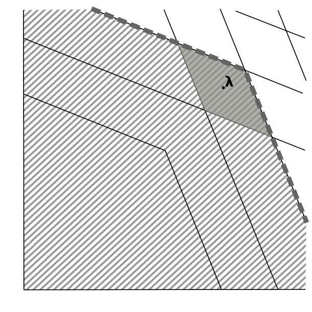
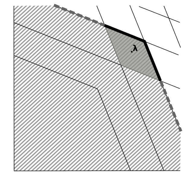
Figure 1. On the left, an example of $\mathcal{R}_{\boldsymbol{\mathfrak{a}}}\left(\boldsymbol{\lambda}\right)$ in striped gray lines and the jumping wall associated to $\boldsymbol{\lambda}$ in thick dotted gray lines. On the right, the corresponding $\mathcal{C}_{\boldsymbol{\mathfrak{a}}}\left(\boldsymbol{\lambda}\right)$ in gray and the corresponding ${\mathcal{C}}$-facets in thick black lines.

Remark 2.7.

It follows from its definition that the region ${\mathcal{R}}_{\boldsymbol{\mathfrak{a}}}(\boldsymbol{\lambda})$ associated to any given point is connected. We do not know whether the same property is satisfied by the constancy region ${\mathcal{C}}_{\boldsymbol{\mathfrak{a}}}(\boldsymbol{\lambda})$.

3. An algorithm to compute jumping numbers and multiplier ideals

In [1] we developed a very simple algorithm to construct sequentially the chain of multiplier ideals

$$\mathcal{O}_{X,O}\supseteq\mathcal{J}(\mathfrak{a}^{\lambda_{0}})\varsupsetneq\mathcal{J}(\mathfrak{a}^{\lambda_{1}})\varsupsetneq\mathcal{J}(\mathfrak{a}^{\lambda_{2}})\varsupsetneq...\varsupsetneq\mathcal{J}(\mathfrak{a}^{\lambda_{i}})\varsupsetneq...$$

associated to a single ideal $\mathfrak{a}\subseteq{\mathcal{O}}_{X,O}$. The key point is the fact proved in [1, Theorem 3.5] that, given any ${\lambda}^{\prime}\in\mathbb{R}_{\geqslant 0}$, the consecutive jumping number is

$$\lambda=\min_{i}\left\{\frac{k_{i}+1+e_{i}^{\lambda^{\prime}}}{e_{i}}\right\},$$

where $D_{{\lambda^{\prime}}}=\sum e_{i}^{{\lambda^{\prime}}}E_{i}$ is the antinef closure of $\left\lfloor\lambda^{\prime}F-K_{\pi}\right\rfloor$. In particular, the algorithm relies heavily on the unloading procedure described in Section 2.1.

The goal in this work is to adapt and extend the aforementioned methods to compute the constancy regions of a tuple of ideals $\boldsymbol{\mathfrak{a}}:=\left(\mathfrak{a}_{1},\dots,\mathfrak{a}_{r}\right)\subseteq\left({\mathcal{O}}_{X,O}\right)^{r}$ and describe the corresponding mixed multiplier ideals. We start by fixing a common log-resolution $\pi:X^{\prime}{\longrightarrow}X$ of $\boldsymbol{\mathfrak{a}}$. Then we have to consider the relative canonical divisor $K_{\pi}=\sum_{i=1}^{s}k_{j}E_{j}$ and the divisors $F_{i}$ in $X^{\prime}$ such that $\mathfrak{a}_{i}\cdot{\mathcal{O}}_{X^{\prime}}={\mathcal{O}}_{X^{\prime}}(-F_{i})$ decomposed as

$$F_{i}=F_{i}^{\rm exc}+F_{i}^{\rm aff}=\sum_{j=1}^{s}e_{i,j}E_{j}+\sum_{j=s+1}^{t}e_{i,j}E_{j}$$

in terms of its exceptional and affine support.

As in the case treated in [1], the key point of our method is how to compare the complete ideals defined by an antinef and a non-antinef divisor. First we recall the following result.

Proposition 3.1.

[1, Corollary 3.4] Let $D_{1},D_{2}$ be two divisors in $X^{\prime}$ such that $D_{1}\leqslant D_{2}$. Then:

• $\pi_{*}\mathcal{O}_{X^{\prime}}(-D_{1})=\pi_{*}\mathcal{O}_{X^{\prime}}(-D_{2})$ if and only if $\widetilde{D_{1}}\geqslant D_{2}$.

• $\pi_{*}\mathcal{O}_{X^{\prime}}(-D_{1})\varsupsetneq\pi_{*}\mathcal{O}_{X^{\prime}}(-D_{2})$ if and only if $v_{i}(\widetilde{D_{1}})<v_{i}(D_{2})$ for some $E_{i}$.

Then we get the following generalization of [1, Corollary 3.4] to the setting of mixed multiplier ideals.

Corollary 3.2.

Let $\boldsymbol{\mathfrak{a}}:=\left(\mathfrak{a}_{1},\dots,\mathfrak{a}_{r}\right)\subseteq({\mathcal{O}}_{X,O})^{r}$ be a tuple of ideals and $\boldsymbol{\lambda},\boldsymbol{\lambda^{\prime}}\in\mathbb{R}^{r}_{\geqslant 0}$. Let $D_{\boldsymbol{\lambda}}=\sum e^{\boldsymbol{\lambda}}_{j}E_{j}$ be the antinef closure of $\left\lfloor\lambda_{1}F_{1}+\cdots+\lambda_{r}F_{r}-K_{\pi}\right\rfloor$. Then:

• $\boldsymbol{\lambda^{\prime}}\in{\mathcal{R}}_{\boldsymbol{\mathfrak{a}}}(\boldsymbol{\lambda})$ if and only if $\lfloor\lambda^{\prime}_{1}e_{1,j}+\cdots+\lambda^{\prime}_{r}e_{r,j}-k_{j}\rfloor\leqslant e^{\boldsymbol{\lambda}}_{j}$ for all $E_{j}$,

With the technical tools stated above we are ready for the main result of this section. Namely, we provide a formula to compute the region associated to any given point that is a generalization of [1, Theorem 3.5] in the context of mixed multiplier ideals.

Theorem 3.3.

Let $\boldsymbol{\mathfrak{a}}:=\left(\mathfrak{a}_{1},\dots,\mathfrak{a}_{r}\right)\subseteq\left(\mathcal{O}_{X,O}\right)^{r}$ be a tuple of ideals and let $D_{{\boldsymbol{\lambda}}}=\sum e_{j}^{{\boldsymbol{\lambda}}}E_{j}$ be the antinef closure of $\left\lfloor\lambda_{1}F_{1}+\cdots+\lambda_{r}F_{r}-K_{\pi}\right\rfloor$ for a given ${\boldsymbol{\lambda}}\in\mathbb{R}^{r}_{\geqslant 0}$. Then the region of $\boldsymbol{\lambda}$ is the rational convex polytope determined by the inequalities

$$e_{1,j}z_{1}+\cdots+e_{r,j}z_{r}<k_{j}+1+e_{j}^{{\boldsymbol{\lambda}}}\,,$$

corresponding to either rupture or dicritical divisors $E_{j}$.

In order to prove the second part of this result, we need to invoke some results on jumping divisors that will be develop in Section 4.

Proof.

It follows from Corollary 3.2 that $\boldsymbol{\lambda^{\prime}}$ is not in the region if and only if there exists $E_{j}$ such that

$$\lfloor\lambda_{1}^{\prime}e_{1,j}+\cdots+\lambda_{r}^{\prime}e_{r,j}-k_{j}\rfloor>e^{\boldsymbol{\lambda}}_{j}.$$

This inequality is equivalent to, $-k_{j}+\lambda_{1}^{\prime}e_{1,j}+\cdots+\lambda_{r}^{\prime}e_{r,j}\geqslant e_{j}^{{\boldsymbol{\lambda}}}+1$ and therefore to $\lambda_{1}^{\prime}e_{1,j}+\cdots+\lambda_{r}^{\prime}e_{r,j}\geqslant k_{j}+1+e_{j}^{\boldsymbol{\lambda}}$.

To finish the proof, we have to prove that we only need to consider the rupture or dicritical divisors. Let $H_{j}:e_{1,j}z_{1}+\cdots+e_{r,j}z_{r}=k_{j}+1+e_{j}^{{\boldsymbol{\lambda}}}$ be the hyperplane associated to the divisor $E_{j}$ considered above. Then, among all the exceptional divisors $E_{i}$ such that $e_{1,i}z_{1}+\cdots+e_{r,i}z_{r}=k_{i}+1+e_{j}^{{\boldsymbol{\lambda}}}$ gives the same hyperplane $H$, we may find a rupture or dicritical divisor by Theorem 4.14. ∎

Remark 3.4.

When $X$ has a rational singularity at $O$, we may have a strict inclusion $\mathcal{O}_{X,O}\varsupsetneq\mathcal{J}(\boldsymbol{\mathfrak{a}}^{\boldsymbol{\lambda}_{0}})$ for $\boldsymbol{\lambda}_{0}=(0,\dots,0)$. The above result for this case gives a mild generalization of the well-known formula for the region ${\mathcal{R}}_{\boldsymbol{\mathfrak{a}}}(\boldsymbol{\lambda}_{0})$ in the smooth case (see [14] where this region is denoted LCT-polytope). Namely, it is the rational convex polytope determined by the inequalities

$$e_{1,j}z_{1}+\cdots+e_{r,j}z_{r}<k_{j}+1+e_{j}^{{\boldsymbol{\lambda}_{0}}}\,,$$

corresponding to either rupture or dicritical divisors $E_{j}$.

Remark 3.5.

When $X$ is smooth, Cassou-Noguès and Libgober [5, 6] studied the analogous notions of ideals and faces of quasi-adjunction of a tuple of irreducible plane curves. In particular, they obtained a formula for the region associated to any given germ $\phi\in{\mathcal{O}}_{X,O}$ that resembles the one given in Theorem 3.3 (see [5, Proposition 2.2] and [6, Theorem 4.1]).

Corollary 3.6.

Let $\boldsymbol{\mathfrak{a}}:=\left(\mathfrak{a}_{1},\dots,\mathfrak{a}_{r}\right)\subseteq({\mathcal{O}}_{X,O})^{r}$ be a tuple of ideals. Then the region ${\mathcal{R}}_{\boldsymbol{\mathfrak{a}}}(\boldsymbol{\lambda})$ is bounded for any point $\boldsymbol{\lambda}\in\mathbb{R}^{r}_{\geqslant 0}$.

This property enables us to give a recursive way to compute the constancy region ${\mathcal{C}}_{\boldsymbol{\mathfrak{a}}}(\boldsymbol{\lambda})$ from the finitely many constancy regions satisfying ${\mathcal{C}}_{\boldsymbol{\mathfrak{a}}}(\boldsymbol{\lambda^{\prime}})\preccurlyeq{\mathcal{C}}_{\boldsymbol{\mathfrak{a}}}(\boldsymbol{\lambda})$.

Corollary 3.7.

Let $\boldsymbol{\mathfrak{a}}:=\left(\mathfrak{a}_{1},\dots,\mathfrak{a}_{r}\right)\subseteq({\mathcal{O}}_{X,O})^{r}$ be a tuple of ideals. Given $\boldsymbol{\lambda}\in\mathbb{R}^{r}_{\geqslant 0}$, there exists finitely many points $\boldsymbol{\lambda}_{1},\dots,\boldsymbol{\lambda}_{k}\in\mathbb{R}^{r}_{\geqslant 0}$ such that

(3.1) $${\mathcal{C}}_{\boldsymbol{\mathfrak{a}}}(\boldsymbol{\lambda})={\mathcal{R}}_{\boldsymbol{\mathfrak{a}}}(\boldsymbol{\lambda})\backslash\left({\mathcal{R}}_{\boldsymbol{\mathfrak{a}}}(\boldsymbol{\lambda}_{1})\cup\cdots\cup{\mathcal{R}}_{\boldsymbol{\mathfrak{a}}}(\boldsymbol{\lambda}_{k})\right)={\mathcal{R}}_{\boldsymbol{\mathfrak{a}}}(\boldsymbol{\lambda})\backslash\left({\mathcal{C}}_{\boldsymbol{\mathfrak{a}}}(\boldsymbol{\lambda}_{1})\cup\cdots\cup{\mathcal{C}}_{\boldsymbol{\mathfrak{a}}}(\boldsymbol{\lambda}_{k})\right).$$

In particular, ${\mathcal{C}}_{\boldsymbol{\mathfrak{a}}}(\boldsymbol{\lambda}_{1}),\dots,{\mathcal{C}}_{\boldsymbol{\mathfrak{a}}}(\boldsymbol{\lambda}_{k})$ are all the constancy regions that are strictly smaller than ${\mathcal{C}}_{\boldsymbol{\mathfrak{a}}}(\boldsymbol{\lambda})$ using the partial order $\preccurlyeq$.

Remark 3.8.

To obtain a simpler expression in the first equation of (3.1) we may choose $\boldsymbol{\lambda}_{1},\dots,\boldsymbol{\lambda}_{s}\in\mathbb{R}^{r}_{\geqslant 0}$ such that ${\mathcal{C}}_{\boldsymbol{\mathfrak{a}}}(\boldsymbol{\lambda}_{1}),\dots,{\mathcal{C}}_{\boldsymbol{\mathfrak{a}}}(\boldsymbol{\lambda}_{s})$ are the maximal elements among those constancy regions which are strictly smaller than ${\mathcal{C}}_{\boldsymbol{\mathfrak{a}}}(\boldsymbol{\lambda})$ using the partial order $\preccurlyeq$. Then

(3.2) $${\mathcal{C}}_{\boldsymbol{\mathfrak{a}}}(\boldsymbol{\lambda})={\mathcal{R}}_{\boldsymbol{\mathfrak{a}}}(\boldsymbol{\lambda})\backslash\left({\mathcal{R}}_{\boldsymbol{\mathfrak{a}}}(\boldsymbol{\lambda}_{1})\cup\cdots\cup{\mathcal{R}}_{\boldsymbol{\mathfrak{a}}}(\boldsymbol{\lambda}_{s})\right).$$

Theorem 3.3 is one of the key ingredients for the algorithm that we will present in Section 3.1. The other key ingredient comes from a careful study of the ${\mathcal{C}}$-facets of the components of a constancy regions that will show their subtlety.

For simplicity, due to the fact that for a fixed jumping point $\boldsymbol{\lambda}$, for $\varepsilon>0$ sufficiently small any ${\boldsymbol{\lambda^{\prime}}\in\{\boldsymbol{\lambda}-\mathbb{R}_{\geqslant 0}^{r}\}\cap B_{\varepsilon}(\boldsymbol{\lambda})}$ defines the same mixed multiplier ideal, we will denote this mixed multiplier ideal as the one associated to $(1-\varepsilon)\boldsymbol{\lambda}$ for $\varepsilon>0$ sufficiently small.

We start with the following well-known fact.

Lemma 3.9.

Let $\boldsymbol{\mathfrak{a}}:=\left(\mathfrak{a}_{1},\dots,\mathfrak{a}_{r}\right)\subseteq({\mathcal{O}}_{X,O})^{r}$ be a tuple of ideals and $\boldsymbol{\lambda}\in\mathbb{R}^{r}_{\geqslant 0}$ be a point.

1. The interior of a ${\mathcal{C}}$-facet, as a subspace of its supporting hyperplane, is non-empty.

2. Any constancy region ${\mathcal{C}}_{\boldsymbol{\mathfrak{a}}}(\boldsymbol{\lambda})$ different from the constancy region associated to the origin, has non-empty intersection with the interior of some ${\mathcal{C}}$-facets.

3. Any interior point $\boldsymbol{\lambda^{\prime}}$ of a ${\mathcal{C}}$-facet of ${\mathcal{C}}_{\boldsymbol{\mathfrak{a}}}(\boldsymbol{\lambda})$ satisfies $\mathcal{J}(\boldsymbol{\mathfrak{a}}^{(1-\varepsilon)\boldsymbol{\lambda^{\prime}}})=\mathcal{J}(\boldsymbol{\mathfrak{a}}^{\boldsymbol{\lambda}})$

Proof.

The key point in the proof of these three statements is that, for all $\varepsilon>0$, we have that $B_{\varepsilon}(\boldsymbol{\lambda})\cap{\mathcal{R}}_{\boldsymbol{\mathfrak{a}}}(\boldsymbol{\lambda})$ contains an open ball $B_{\varepsilon}(\boldsymbol{\mu})$ for some $\boldsymbol{\mu}\in{\mathcal{R}}_{\boldsymbol{\mathfrak{a}}}(\boldsymbol{\lambda})$. To finish the proof of ii) we notice that the inner boundary ${\mathcal{C}}_{\boldsymbol{\mathfrak{a}}}(\boldsymbol{\lambda})\backslash{\mathcal{C}}_{\boldsymbol{\mathfrak{a}}}(\boldsymbol{\lambda})^{\circ}$ provides the points of ${\mathcal{C}}_{\boldsymbol{\mathfrak{a}}}(\boldsymbol{\lambda})$ which are interior points of a ${\mathcal{C}}$-facet of some other constancy region, which is necessarily smaller than ${\mathcal{C}}_{\boldsymbol{\mathfrak{a}}}(\boldsymbol{\lambda})$ using the partial order $\preccurlyeq$. ∎

The key result states that a ${\mathcal{C}}$-facet cannot be crossed by any jumping wall.

Proposition 3.10.

Let $\boldsymbol{\mathfrak{a}}:=\left(\mathfrak{a}_{1},\dots,\mathfrak{a}_{r}\right)\subseteq({\mathcal{O}}_{X,O})^{r}$ be a tuple of ideals. Let $\boldsymbol{\lambda}$ and $\boldsymbol{\lambda^{\prime}}$ be interior points of the same ${\mathcal{C}}$-facet of a constancy region. Then we have $\mathcal{J}\left(\boldsymbol{\mathfrak{a}}^{\boldsymbol{\lambda}}\right)=\mathcal{J}\left(\boldsymbol{\mathfrak{a}}^{\boldsymbol{\lambda^{\prime}}}\right)$.

Once again we need to use some results from Section 4 to prove this fact.

Proof.

Let $H$ be the supporting hyperplane of the ${\mathcal{C}}$-facet containing $\boldsymbol{\lambda}$ and $\boldsymbol{\lambda^{\prime}}$. Notice that both are jumping points coming from the same mixed multiplier ideal, i.e., ${\mathcal{J}\left(\boldsymbol{\mathfrak{a}}^{(1-\varepsilon)\boldsymbol{\lambda}}\right)=\mathcal{J}\left(\boldsymbol{\mathfrak{a}}^{(1-\varepsilon)\boldsymbol{\lambda^{\prime}}}\right)}$. For simplicity we take a point $\boldsymbol{\mu}$ as a representative of the constancy region of this ideal. Now, let $D_{\boldsymbol{\mu}}=\sum e_{j}^{\boldsymbol{\mu}}E_{j}$ be the antinef closure of $\lfloor\mu_{1}F_{1}+\cdots+\mu_{r}F_{r}-K_{\pi}\rfloor$. Consider the reduced divisor $G$ supported on those exceptional components $E_{j}$ such that the hyperplane $H$ has equation

$$\lambda_{1}e_{1,j}+\cdots+\lambda_{r}e_{r,j}=k_{j}+1+e_{j}^{{\boldsymbol{\mu}}}\,.$$

Then, using Lemma 4.6 and Proposition 4.10 we have

$$\mathcal{J}\left(\boldsymbol{\mathfrak{a}}^{\boldsymbol{\lambda}}\right)=\pi_{*}\mathcal{O}_{X^{\prime}}(-D_{(1-\varepsilon)\boldsymbol{\lambda}}-G)=\mathcal{J}\left(\boldsymbol{\mathfrak{a}}^{\boldsymbol{\lambda^{\prime}}}\right).$$

∎

3.1. An algorithm to compute the constancy regions

The algorithm that we are going to present is a generalization of the one given in [1, Algorithm 3.8] that we briefly recall. Given an ideal $\mathfrak{a}\subseteq{\mathcal{O}}_{X,O}$, we construct sequentially the chain of multiplier ideals

$$\mathcal{O}_{X,O}\supseteq\mathcal{J}(\mathfrak{a}^{\lambda_{0}})\varsupsetneq\mathcal{J}(\mathfrak{a}^{\lambda_{1}})\varsupsetneq\mathcal{J}(\mathfrak{a}^{\lambda_{2}})\varsupsetneq...\varsupsetneq\mathcal{J}(\mathfrak{a}^{\lambda_{i}})\varsupsetneq...$$

The starting point is to compute the multiplier ideal associated to $\lambda_{0}=0$ by means of the antinef closure $D_{\lambda_{0}}=\sum e_{i}^{\lambda_{0}}E_{i}$ of $\lfloor-K_{\pi}\rfloor$ using the unloading procedure described in Section 2.1. The log-canonical threshold is

$$\lambda_{1}=\min_{i}\left\{\frac{k_{i}+1+e_{i}^{\lambda_{0}}}{e_{i}}\right\}\,.$$

so we may describe its associated multiplier ideal $\mathcal{J}(\mathfrak{a}^{\lambda_{1}})$ just computing the antinef closure $D_{\lambda_{1}}=\sum e_{i}^{\lambda_{1}}E_{i}$ of $\lfloor\lambda_{1}F-K_{\pi}\rfloor$ using the unloading procedure. By [1, Theorem 3.5], the next jumping number is

$$\lambda_{2}=\min_{i}\left\{\frac{k_{i}+1+e_{i}^{\lambda_{1}}}{e_{i}}\right\}.$$

Then we only have to follow the same strategy: the antinef closure $D_{\lambda_{2}}$ of $\lfloor\lambda_{2}F-K_{\pi}\rfloor$, i.e., the multiplier ideal $\mathcal{J}(\mathfrak{a}^{\lambda_{2}})$, allows us to compute $\lambda_{3}$ and so on.

We may interpret that at each step of the algorithm, the jumping number $\lambda_{i}$ allows us to compute its region, and equivalently its constancy region $[\lambda_{i},\lambda_{i+1})$. The boundary of this constancy region gives us the next jumping number $\lambda_{i+1}$. In particular we have a one-to-one correspondence between the constancy regions of the ideal $\mathfrak{a}$ and the jumping numbers.

The algorithm for mixed multiplier ideals is more involved. It starts with the computation of the mixed multiplier ideal associated to $\boldsymbol{\lambda}_{0}=(0,\dots,0)$, using the unloading procedure. The region ${\mathcal{R}}_{\boldsymbol{\mathfrak{a}}}(\boldsymbol{\lambda}_{0})$ is described by means of the formula given in Theorem 3.3. In this case the region coincides with the constancy region ${\mathcal{C}}_{\boldsymbol{\mathfrak{a}}}(\boldsymbol{\lambda}_{0})$, so we have a nice description of its boundary. For each ${\mathcal{C}}$-facet, using Proposition 3.10, we may take a single point as a representative. The next step of the algorithm is to compute the mixed multiplier ideals of these points in order to describe their corresponding regions, using Theorem 3.3 once again. Then we compute the corresponding constancy regions and their ${\mathcal{C}}$-facets and we follow the same strategy.

Roughly speaking, our strategy is to consider a discrete set of points comprising one interior point of each ${\mathcal{C}}$-facet. This gives a surjective correspondence with the partially ordered set of constancy regions. This correspondence is far from being one-to-one as in the case of a single ideal. To keep track of these points we will consider two sets $N$ and $D$. $N$ will contain the points for which we still have to compute the corresponding region and, once this region has been computed, we move it to $D$. In particular, we will start with $N=\{\boldsymbol{\lambda}_{0}\}$ and $D=\emptyset$ the empty set.

Algorithm 3.11.

(Constancy regions and mixed multiplier ideals)

Input: a common log-resolution of the tuple of ideals $\boldsymbol{\mathfrak{a}}=\left(\mathfrak{a}_{1},\dots,\mathfrak{a}_{r}\right)\subseteq({\mathcal{O}}_{X,O})^{r}$.

Output: list of constancy regions of $\boldsymbol{\mathfrak{a}}$ and their corresponding mixed multiplier ideals.

Set $N=\{\boldsymbol{\lambda}_{0}=(0,\dots,0)\}$ and $D=\emptyset$. From $j=0$ , incrementing by $1$

• :

  1. Choosing a convenient point in the set $N$:

     • Pick $\boldsymbol{\lambda}_{j}$ the first point in the set $N$ and compute its region ${\mathcal{R}}_{\boldsymbol{\mathfrak{a}}}(\boldsymbol{\lambda}_{j})$ using Theorem 3.3.

     • If there is some $\boldsymbol{\lambda}\in N$ such that $\boldsymbol{\lambda}\in{\mathcal{R}}_{\boldsymbol{\mathfrak{a}}}(\boldsymbol{\lambda}_{j})$ and $\mathcal{J}(\mathfrak{a}^{\boldsymbol{\lambda}})\neq\mathcal{J}(\mathfrak{a}^{\boldsymbol{\lambda}_{j}})$ then put $\boldsymbol{\lambda}$ first in the list $N$ and repeat this step $(j.1)$. Otherwise continue with step $(j.2)$.

  2. Checking out whether the region has been already computed:

     • If some $\boldsymbol{\lambda}\in D$ satisfies $\mathcal{J}(\mathfrak{a}^{\boldsymbol{\lambda}})=\mathcal{J}(\mathfrak{a}^{\boldsymbol{\lambda}_{j}})$ then go to step $(j.4)$. Otherwise continue with step $(j.3)$.

  3. Picking new points for which we have to compute its region:

     • Compute

       $${\mathcal{C}}(j)={\mathcal{R}}_{\boldsymbol{\mathfrak{a}}}(\boldsymbol{\lambda}_{j})\backslash\left({\mathcal{R}}_{\boldsymbol{\mathfrak{a}}}(\boldsymbol{\lambda}_{1})\cup\cdots\cup{\mathcal{R}}_{\boldsymbol{\mathfrak{a}}}(\boldsymbol{\lambda}_{j-1})\right).$$

     • For each connected component of ${\mathcal{C}}(j)$ compute its outer facets.

     • Pick one interior point in each outer facet of ${\mathcal{C}}(j)$ and add them as the last point in $N$.

  4. Update the sets $N$ and $D$:

     • Delete $\boldsymbol{\lambda}_{j}$ from $N$ and add $\boldsymbol{\lambda}_{j}$ as the last point in $D$.

Remark 3.12.

Several points of the algorithm require a comparison between mixed multiplier ideals (an inequality in step $(j.1)$ and an equality in step $(j.2)$). This can be done computing antinef closures of divisors using the unloading procedure. For the computation of the region ${\mathcal{R}}_{\boldsymbol{\mathfrak{a}}}(\boldsymbol{\lambda})$ (steps $(j.1)$ and $(j.3)$) we use Theorem 3.3.

Remark 3.13.

Step $(j.1)$ is equivalent to choosing a point whose constancy region is a minimal element by the order $\preccurlyeq$ among those associated to the points in the set $N$. Any finite subset endowed with a partial ordering has some minimal element, thus there exists a convenient point in the set $N$ that allows to continue with step $(j.2)$.

Lemma 3.14.

At each step $j$, the algorithm overcomes step $(j.1)$ and provides updated sets $N$ and $D$.

Theorem 3.15.

The constancy region of the point $\boldsymbol{\lambda}_{j}$ chosen at step $(j.1)$ is computed at step $(j.3)$ of the algorithm, i.e., ${\mathcal{C}}(j)={\mathcal{C}}_{\boldsymbol{\mathfrak{a}}}(\boldsymbol{\lambda}_{j})$, and one interior point for each ${\mathcal{C}}$-facet of ${\mathcal{C}}_{\boldsymbol{\mathfrak{a}}}(\boldsymbol{\lambda}_{j})$ is added to the set $N$.

Proof.

We argue by induction on $j$. For the case $j=1$ the statement holds since we pick $\boldsymbol{\lambda}_{1}=\boldsymbol{\lambda}_{0}$ at step $(1.1)$ and step $(1.3)$ is performed.

Now assume that the statement is true all the steps up to $j-1$. We want to prove it for step $j$. Without loss of generality we may assume that step $(j.3)$ must be performed, so $\mathcal{J}(\mathfrak{a}^{\boldsymbol{\lambda}_{i}})\neq\mathcal{J}(\mathfrak{a}^{\boldsymbol{\lambda}_{j}})$ for all $1\leqslant i\leqslant j-1$. Notice that, by equation (3.2), ${\mathcal{C}}(j)={\mathcal{C}}_{\boldsymbol{\mathfrak{a}}}(\boldsymbol{\lambda}_{j})$ is equivalent to the fulfillment of the following two conditions:

• Each $\boldsymbol{\lambda}_{i}$, $1\leqslant i\leqslant j-1$, satisfies either ${\mathcal{C}}_{\boldsymbol{\mathfrak{a}}}(\boldsymbol{\lambda}_{i})\preccurlyeq{\mathcal{C}}_{\boldsymbol{\mathfrak{a}}}(\boldsymbol{\lambda}_{j})$ or both constancy regions are not related by the partial order.

• Consider a set $\{\boldsymbol{\mu}_{1},\dots,\boldsymbol{\mu}_{s}\}\subset\mathbb{R}_{\geqslant 0}^{r}$ of representatives of the constancy regions which are maximal elements among those constancy regions smaller than ${\mathcal{C}}_{\boldsymbol{\mathfrak{a}}}(\boldsymbol{\lambda}_{j})$. Then, for each $k\in\{1,\dots,s\}$ there is some $i_{k}\in\{1,\dots,j-1\}$ such that ${\mathcal{C}}_{\boldsymbol{\mathfrak{a}}}(\boldsymbol{\lambda}_{i_{k}})\preccurlyeq{\mathcal{C}}_{\boldsymbol{\mathfrak{a}}}(\boldsymbol{\mu}_{k})$.

First we are going to prove that condition a) is satisfied. Assume the contrary, i.e. there exists $i<j$ with ${\mathcal{C}}_{\boldsymbol{\mathfrak{a}}}(\boldsymbol{\lambda}_{i})\succ{\mathcal{C}}_{\boldsymbol{\mathfrak{a}}}(\boldsymbol{\lambda}_{j})$, that is ${\mathcal{R}}_{\boldsymbol{\mathfrak{a}}}(\boldsymbol{\lambda}_{i})\varsupsetneq{\mathcal{R}}_{\boldsymbol{\mathfrak{a}}}(\boldsymbol{\lambda}_{j})$. Assume that $\boldsymbol{\lambda}_{j}$ was added to $N$ at step $m<j$. Hence, by induction hypothesis $\boldsymbol{\lambda}_{j}$ is an interior point of some ${\mathcal{C}}$-facet of ${\mathcal{R}}_{\boldsymbol{\mathfrak{a}}}(\boldsymbol{\lambda}_{m})$, and in particular ${\mathcal{R}}_{\boldsymbol{\mathfrak{a}}}(\boldsymbol{\lambda}_{m})\subseteq{\mathcal{R}}_{\boldsymbol{\mathfrak{a}}}(\boldsymbol{\lambda}_{j})$. Thus ${\mathcal{R}}_{\boldsymbol{\mathfrak{a}}}(\boldsymbol{\lambda}_{m})\varsubsetneq{\mathcal{R}}_{\boldsymbol{\mathfrak{a}}}(\boldsymbol{\lambda}_{i})$, i.e. ${\mathcal{C}}_{\boldsymbol{\mathfrak{a}}}(\boldsymbol{\lambda}_{m})\prec{\mathcal{C}}_{\boldsymbol{\mathfrak{a}}}(\boldsymbol{\lambda}_{i})$. We distinguish two cases:

• If $i<m$ we get a contradiction with the induction hypothesis at step $m$ since condition a) is not fulfilled.

• If $i>m$, we have that $\boldsymbol{\lambda}_{j}$ already belongs to $N$ at step $i$. This contradicts the requirement of step $(i.1)$ which says that $\boldsymbol{\lambda}_{j}$ should be treated before $\boldsymbol{\lambda}_{i}$.

Finally we prove condition b). Assume the contrary, i.e there exists $\boldsymbol{\mu}_{i}$ whose constancy region is not dominated by any ${\mathcal{C}}_{\boldsymbol{\mathfrak{a}}}(\boldsymbol{\lambda}_{k})$, $1\leqslant k\leqslant j-1$. Without loss of generality we may assume that the segment $\overline{\boldsymbol{\lambda}_{0}\boldsymbol{\mu}_{i}}$ intersect the jumping walls at interior points of the ${\mathcal{C}}$-facets, namely in the jumping points $\boldsymbol{\lambda}_{0}=\boldsymbol{\nu}_{1},\boldsymbol{\nu}_{2},\dots,\boldsymbol{\nu}_{m}=\boldsymbol{\mu}_{i}$ with $\boldsymbol{\nu}_{k}\in\overline{{\mathcal{C}}_{\boldsymbol{\mathfrak{a}}}(\boldsymbol{\nu}_{k-1})}$, and thus $\boldsymbol{\nu}_{k-1}\in{\mathcal{R}}_{\boldsymbol{\mathfrak{a}}}(\boldsymbol{\nu}_{k})$.

By induction hypothesis, representatives of each constancy region $\{{\mathcal{C}}_{\boldsymbol{\mathfrak{a}}}(\boldsymbol{\nu}_{1}),\dots,{\mathcal{C}}_{\boldsymbol{\mathfrak{a}}}(\boldsymbol{\nu}_{m^{\prime}})\}$, $m^{\prime}<m$, are added to $N$ at some steps before step $j$, being $\boldsymbol{\lambda^{\prime}}$ the last representative. Hence, we still have $\boldsymbol{\lambda^{\prime}}\in N$ at step $j$ and

$${\mathcal{R}}_{\boldsymbol{\mathfrak{a}}}(\boldsymbol{\lambda^{\prime}})={\mathcal{R}}_{\boldsymbol{\mathfrak{a}}}(\boldsymbol{\nu}_{m^{\prime}})\subseteq{\mathcal{R}}_{\boldsymbol{\mathfrak{a}}}(\boldsymbol{\mu}_{i})\subsetneq{\mathcal{R}}_{\boldsymbol{\mathfrak{a}}}(\boldsymbol{\lambda}_{j}).$$

This contradicts the requirement of step $(j.1)$ for $\boldsymbol{\lambda}_{j}$. ∎

As a consequence of Theorem 3.15 we obtain the following

Corollary 3.16.

At step $j$ of the algorithm, we have that:

• The set $D$ contains at least a representative of each constancy region inside ${\mathcal{R}}_{\boldsymbol{\mathfrak{a}}}(\boldsymbol{\lambda}_{j})$.

• The set $D$ contains a representative of all ${\mathcal{C}}$-facets inside ${\mathcal{R}}_{\boldsymbol{\mathfrak{a}}}(\boldsymbol{\lambda}_{j})$.

• A complete description of the jumping walls inside ${\mathcal{R}}_{\boldsymbol{\mathfrak{a}}}(\boldsymbol{\lambda}_{j})$ is obtained by intersecting the region ${\mathcal{R}}_{\boldsymbol{\mathfrak{a}}}(\boldsymbol{\lambda}_{j})$ with the jumping walls associated to the points $\boldsymbol{\lambda}_{1},\dots,\boldsymbol{\lambda}_{j-1}$.

Proof.

From the proof of Theorem 3.15 we infer that at step $j$, the maximal elements among all the constancy regions inside ${\mathcal{R}}_{\boldsymbol{\mathfrak{a}}}(\boldsymbol{\lambda}_{j})$ have already representants $\boldsymbol{\lambda}_{i_{1}},\dots,\boldsymbol{\lambda}_{i_{s}}$ in $D$, $i_{1}<\cdots<i_{s}<j$. Arguing by reverse induction with any of these points $\boldsymbol{\lambda}_{i_{k}}$, the first claim follows.

Now, the statement of Theorem 3.15 asserts that at each step $i$ of the algorithm, a representative of each ${\mathcal{C}}$-facet of ${\mathcal{C}}_{\boldsymbol{\mathfrak{a}}}(\boldsymbol{\lambda}_{i})$ is added to $N$. If we only take into account the points $\boldsymbol{\lambda}_{i}$ of constancy regions inside ${\mathcal{R}}_{\boldsymbol{\mathfrak{a}}}(\boldsymbol{\lambda}_{j})$, the subsequent representatives in ${\mathcal{C}}$-facets still lying inside ${\mathcal{R}}_{\boldsymbol{\mathfrak{a}}}(\boldsymbol{\lambda}_{j})$ must be treated (and added to $D$) before $\boldsymbol{\lambda}_{j}$, in virtue of step $(j.1)$ of the algorithm.

Part iii) of the statement is a direct consequence of claim i). ∎

Remark 3.17.

Each point $\boldsymbol{\lambda}$ included in $N$ at some step of the algorithm is treated after a finite number of steps and added to $D$. Indeed, the order of incorporation of the points in $N$ is preserved unless step $(j.1)$ priorizes some other point. This happens only a finite amount of times since there is only a finite number of constancy regions inside any given region.

Proposition 3.18.

Once a point $\boldsymbol{\lambda}\in\mathbb{R}_{\geqslant 0}^{r}$ is fixed, a set $D$ which includes a representative of all constancy regions in the compact $(\boldsymbol{\lambda}_{0}+\mathbb{R}_{\geqslant 0}^{r})\cap(\boldsymbol{\lambda}-\mathbb{R}_{\geqslant 0}^{r})$ is achieved after a finite number of steps of the algorithm.

Proof.

Observe that $(\boldsymbol{\lambda}_{0}+\mathbb{R}_{\geqslant 0}^{r})\cap(\boldsymbol{\lambda}-\mathbb{R}_{\geqslant 0}^{r})\subseteq{\mathcal{R}}_{\boldsymbol{\mathfrak{a}}}(\boldsymbol{\lambda})$. In virtue of Corollary 3.16 and Remark 3.17, we only have to prove that some representative of ${\mathcal{C}}_{\boldsymbol{\mathfrak{a}}}(\boldsymbol{\lambda})$ is added to $N$ at some step. We may take $\boldsymbol{\lambda^{\prime}}\in{\mathcal{C}}_{\boldsymbol{\mathfrak{a}}}(\boldsymbol{\lambda})$ such that the segment $\overline{\boldsymbol{\lambda}_{0}\boldsymbol{\lambda^{\prime}}}$ intersects the jumping walls at interior points of ${\mathcal{C}}$-facets, namely in the jumping points $\boldsymbol{\lambda}_{0}=\boldsymbol{\nu}_{1},\boldsymbol{\nu}_{2},\dots,\boldsymbol{\nu}_{m}=\boldsymbol{\lambda^{\prime}}$. The algorithm starts with $\boldsymbol{\nu}_{1}$ and incorporates $\boldsymbol{\nu}_{2}$ to $N$. Since $\boldsymbol{\nu}_{k}\in\overline{{\mathcal{C}}_{\boldsymbol{\mathfrak{a}}}(\boldsymbol{\nu}_{k-1})}$, once $\boldsymbol{\nu}_{k}$ is selected at some finite step $i_{k}$, $\boldsymbol{\nu}_{k+1}$ is added to $N$ at this same step. Hence, $\boldsymbol{\lambda^{\prime}}$ is selected at some step $(j.1)$. Notice that this implies that no point in $N$ lies in ${\mathcal{R}}_{\boldsymbol{\mathfrak{a}}}(\boldsymbol{\lambda^{\prime}})={\mathcal{R}}_{\boldsymbol{\mathfrak{a}}}(\boldsymbol{\lambda})$, i.e. $N\cap{\mathcal{R}}_{\boldsymbol{\mathfrak{a}}}(\boldsymbol{\lambda})=\emptyset$.

Conversely, if at some step $j$ $N\cap{\mathcal{R}}_{\boldsymbol{\mathfrak{a}}}(\boldsymbol{\lambda})=\emptyset$, then the new $N$ obtained at any forthcoming step still satisfies $N\cap{\mathcal{R}}_{\boldsymbol{\mathfrak{a}}}(\boldsymbol{\lambda})=\emptyset$. If some $\boldsymbol{\lambda}_{i}\not\in{\mathcal{R}}_{\boldsymbol{\mathfrak{a}}}(\boldsymbol{\lambda})$ with $i>j$ is chosen at step $(i.1)$, any new point $\boldsymbol{\mu}$ added to $N$ at step $(i.3)$ satisfies $\mathcal{J}(\boldsymbol{\mathfrak{a}}^{\boldsymbol{\mu}})\varsubsetneq\mathcal{J}(\boldsymbol{\mathfrak{a}}^{\boldsymbol{\lambda}_{i}})\nsupseteq\mathcal{J}(\boldsymbol{\mathfrak{a}}^{\boldsymbol{\lambda}})$ and hence $\mathcal{J}(\boldsymbol{\mathfrak{a}}^{\boldsymbol{\mu}})\nsupseteq\mathcal{J}(\boldsymbol{\mathfrak{a}}^{\boldsymbol{\lambda}})$, equivalently $\boldsymbol{\mu}\not\in{\mathcal{R}}_{\boldsymbol{\mathfrak{a}}}(\boldsymbol{\lambda})$. Since the algorithm starts with $\boldsymbol{\lambda}_{1}=\boldsymbol{\lambda}_{0}\in{\mathcal{R}}_{\boldsymbol{\mathfrak{a}}}(\boldsymbol{\lambda})$, we may conclude that at a step where $N\cap{\mathcal{R}}_{\boldsymbol{\mathfrak{a}}}(\boldsymbol{\lambda})=\emptyset$ necessarily the set $D$ obtained at that step contains a representative of ${\mathcal{R}}_{\boldsymbol{\mathfrak{a}}}(\boldsymbol{\lambda})$. ∎

We present the following simple example to highlight the nuances of the procedure. In the example, step $(j.1)$ is performed when computing the region associated to the point $\boldsymbol{\lambda}_{5}$ and step $(j.2)$ is performed for the points $\boldsymbol{\lambda}_{2}$, $\boldsymbol{\lambda}_{4}$, $\boldsymbol{\lambda}_{7}$ and $\boldsymbol{\lambda}_{8}$. In particular, step $(j.2)$ is included to avoid too many computations.

Example 3.19.

Consider the following set of ideals $\boldsymbol{\mathfrak{a}}=(\mathfrak{a}_{1},\mathfrak{a}_{2})$ with $\mathfrak{a}_{1}=(x^{3},y^{7})$ and $\mathfrak{a}_{2}=(x,y^{2})$ on a smooth surface $X$. We represent the relative canonical divisor $K_{\pi}$ and $F_{1}$ and $F_{2}$ in the dual graph as follows:

Vertex ordering	$K_{\pi}$	$(F_{1},F_{2})$

The blank dots correspond to dicritical divisors in one of the ideals and their excesses are represented by broken arrows. For simplicity we will collect the values of any divisor in a vector. Namely, we have $K_{\pi}=(1,2,3,6,9)$, $F_{1}=(3,6,7,14,21)$ and $F_{2}=(1,2,2,4,6)$. In the algorithm we will have to perform several times unloading steps, so we will have to consider the intersection matrix $M=(E_{i}\cdot E_{j})_{1\leqslant i,j\leqslant 5}$

$$M=\left(\begin{array}[]{ccccc}-2&1&0&0&0\\ \vskip 6.0pt plus 2.0pt minus 2.0pt\cr 1&-4&0&0&1\\ \vskip 6.0pt plus 2.0pt minus 2.0pt\cr 0&0&-2&1&0\\ \vskip 6.0pt plus 2.0pt minus 2.0pt\cr 0&0&1&-2&1\\ \vskip 6.0pt plus 2.0pt minus 2.0pt\cr 0&1&0&1&-1\end{array}\right)\,.$$

Notice that $E_{2}$ and $E_{5}$ are the only dicritical divisors. Then, as a consequence of Theorem 3.3, the region of a given point $\boldsymbol{\lambda}=(\lambda_{1},\lambda_{2})$ is defined by

$$\begin{array}[]{lcr}6z_{1}+2z_{2}&<&2+1+e_{2}^{\boldsymbol{\lambda}}\,,\\ 21z_{1}+6z_{2}&<&9+1+e_{5}^{\boldsymbol{\lambda}}\,.\end{array}$$

We keep track of what we have to compute with the set $N$ that for the moment will only contain $\boldsymbol{\lambda}_{0}=(0,0)$. The set $D$ that keeps track of the points that we have already computed will be empty since we have not computed anything yet.

$\bullet$ Step 0. We start computing the multiplier ideal corresponding to $\boldsymbol{\lambda}_{0}=(0,0)$. Namely, the antinef closure of the divisor $\lfloor 0F_{1}+0F_{2}-K_{\pi}\rfloor$ is $D_{\boldsymbol{\lambda}_{0}}=0$. The corresponding region $\mathcal{R}_{\boldsymbol{\mathfrak{a}}}(\boldsymbol{\lambda}_{0})$ is given by the inequalities

$$\begin{array}[]{lcr}6z_{1}+2z_{2}&<&3,\\ 21z_{1}+6z_{2}&<&10.\end{array}$$

Notice that the constancy region $\mathcal{C}_{\boldsymbol{\mathfrak{a}}}(\boldsymbol{\lambda}_{0})$ coincides with $\mathcal{R}_{\boldsymbol{\mathfrak{a}}}(\boldsymbol{\lambda}_{0})$. Its boundary, i.e. the corresponding jumping wall, has two $\mathcal{C}$-facets so, according to Proposition 3.10, we only need to consider an interior point of each $\mathcal{C}$-facet in order to continue our procedure. For simplicity we consider the barycenters $\left(\frac{1}{6},1\right)$ and $\left(\frac{17}{42},\frac{1}{4}\right)$ corresponding to each segment.

• $N=\{\left(\frac{1}{6},1\right),\left(\frac{17}{42},\frac{1}{4}\right)\}$.

• $D=\{\left(0,0\right)\}$.

$\bullet$ Step 1. We pick the first point $\boldsymbol{\lambda}_{1}:=\left(\frac{1}{6},1\right)$ in $N$ and we compute its multiplier ideal. Namely, $\lfloor\frac{1}{6}F_{1}+F_{2}-K_{\pi}\rfloor=(0,1,0,0,0)$ and its antinef closure is $D_{\boldsymbol{\lambda}_{1}}=(1,1,1,2,3)$, so the region $\mathcal{R}_{\boldsymbol{\mathfrak{a}}}(\boldsymbol{\lambda}_{1})$ is given by the inequalities

$$\begin{array}[]{lcr}6z_{1}+2z_{2}&<&4,\\ 21z_{1}+6z_{2}&<&13.\end{array}$$

The constancy region $\mathcal{C}_{\boldsymbol{\mathfrak{a}}}(\boldsymbol{\lambda}_{1})=\mathcal{R}_{\boldsymbol{\mathfrak{a}}}(\boldsymbol{\lambda}_{1})\backslash\mathcal{R}_{\boldsymbol{\mathfrak{a}}}(\boldsymbol{\lambda}_{0})$ has two $\mathcal{C}$-facets for which we pick the interior points $\left(\frac{1}{6},\frac{3}{2}\right)$ and $\left(\frac{10}{21},\frac{1}{2}\right)$ respectively. Then, the sets $N$ and $D$ are:

• $N=\{\left(\frac{17}{42},\frac{1}{4}\right),\left(\frac{1}{6},\frac{3}{2}\right),\left(\frac{10}{21},\frac{1}{2}\right)\}$.

• $D=\{\left(0,0\right),\left(\frac{1}{6},1\right)\}$.

$\bullet$ Step 2. The point $\boldsymbol{\lambda}_{2}:=\left(\frac{17}{42},\frac{1}{4}\right)$ satisfies $\mathcal{J}(\boldsymbol{\mathfrak{a}}^{\boldsymbol{\lambda}_{2}})=\mathcal{J}(\boldsymbol{\mathfrak{a}}^{\boldsymbol{\lambda}_{1}})$, so they have the same region. In order to keep track of all the $\mathcal{C}$-facets we have to consider this point as well, so the sets $N$ and $D$ that we get after this step are:

• $N=\{\left(\frac{1}{6},\frac{3}{2}\right),\left(\frac{10}{21},\frac{1}{2}\right)\}$.

• $D=\{\left(0,0\right),\left(\frac{1}{6},1\right),\left(\frac{17}{42},\frac{1}{4}\right)\}$.

$\bullet$ Step 3. We pick $\boldsymbol{\lambda}_{3}:=\left(\frac{1}{6},\frac{3}{2}\right)$. We have $\lfloor\frac{1}{6}F_{1}+\frac{3}{2}F_{2}-K_{\pi}\rfloor=(1,2,1,2,3)$ and its antinef closure is $D_{\boldsymbol{\lambda}_{3}}=(1,2,2,4,6)$, so the region $\mathcal{R}_{\boldsymbol{\mathfrak{a}}}(\boldsymbol{\lambda}_{3})$ is given by the inequalities

$$\begin{array}[]{lcr}6z_{1}+2z_{2}&<&5,\\ 21z_{1}+6z_{2}&<&16.\end{array}$$

The constancy region $\mathcal{C}_{\boldsymbol{\mathfrak{a}}}(\boldsymbol{\lambda}_{3})=\mathcal{R}_{\boldsymbol{\mathfrak{a}}}(\boldsymbol{\lambda}_{3})\backslash(\mathcal{R}_{\boldsymbol{\mathfrak{a}}}(\boldsymbol{\lambda}_{0})\cup\mathcal{R}_{\boldsymbol{\mathfrak{a}}}(\boldsymbol{\lambda}_{1})\cup\mathcal{R}_{\boldsymbol{\mathfrak{a}}}(\boldsymbol{\lambda}_{3}))=\mathcal{R}_{\boldsymbol{\mathfrak{a}}}(\boldsymbol{\lambda}_{3})\backslash\mathcal{R}_{\boldsymbol{\mathfrak{a}}}(\boldsymbol{\lambda}_{1})$ has two $\mathcal{C}$-facets for which we pick the interior points $\left(\frac{1}{6},2\right)$ and $\left(\frac{23}{42},\frac{3}{4}\right)$ respectively. Then, the sets $N$ and $D$ are:

• $N=\{\left(\frac{10}{21},\frac{1}{2}\right),\left(\frac{1}{6},2\right),\left(\frac{23}{42},\frac{3}{4}\right)\}$.

• $D=\{\left(0,0\right),\left(\frac{1}{6},1\right),\left(\frac{17}{42},\frac{1}{4}\right),\left(\frac{1}{6},\frac{3}{2}\right)\}$.

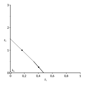
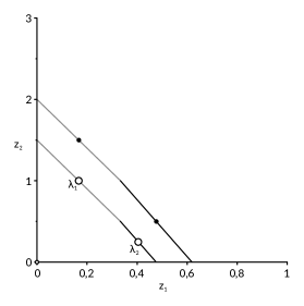
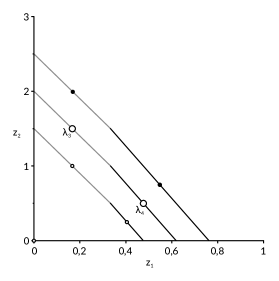
Figure 2. Constancy regions associated to $\boldsymbol{\lambda}_{0}$, $\boldsymbol{\lambda}_{1}$ (equivalently $\boldsymbol{\lambda}_{2}$) and $\boldsymbol{\lambda}_{3}$ (equivalently $\boldsymbol{\lambda}_{4}$).

$\bullet$ Step 4. The point $\boldsymbol{\lambda}_{4}:=\left(\frac{10}{21},\frac{1}{2}\right)$ satisfies $\mathcal{J}(\boldsymbol{\mathfrak{a}}^{\boldsymbol{\lambda}_{4}})=\mathcal{J}(\boldsymbol{\mathfrak{a}}^{\boldsymbol{\lambda}_{3}})$ so they have the same region. We update the sets $N$ and $D$ to obtain:

• $N=\{\left(\frac{1}{6},2\right),\left(\frac{23}{42},\frac{3}{4}\right)\}$.

• $D=\{\left(0,0\right),\left(\frac{1}{6},1\right),\left(\frac{17}{42},\frac{1}{4}\right),\left(\frac{1}{6},\frac{3}{2}\right),\left(\frac{10}{21},\frac{1}{2}\right)\}$.

$\bullet$ Step 5. We have that the region associated to $\left(\frac{23}{42},\frac{3}{4}\right)$ is contained in the region of $\left(\frac{1}{6},2\right)$. It is for this reason that we will consider first the point $\boldsymbol{\lambda}_{5}:=\left(\frac{23}{42},\frac{3}{4}\right)$. We have $\lfloor\frac{23}{42}F_{1}+\frac{3}{4}F_{2}-K_{\pi}\rfloor=(1,2,2,4,7)$ and its antinef closure is $D_{\boldsymbol{\lambda}_{5}}=(1,2,3,5,7)$ so the region $\mathcal{R}_{\boldsymbol{\mathfrak{a}}}(\boldsymbol{\lambda}_{3})$ is given by the inequalities

$$\begin{array}[]{lcr}6z_{1}+2z_{2}&<&5,\\ 21z_{1}+6z_{2}&<&17.\end{array}$$

The constancy region $\mathcal{C}_{\boldsymbol{\mathfrak{a}}}(\boldsymbol{\lambda}_{5})=\mathcal{R}_{\boldsymbol{\mathfrak{a}}}(\boldsymbol{\lambda}_{5})\backslash\mathcal{R}_{\boldsymbol{\mathfrak{a}}}(\boldsymbol{\lambda}_{3})$ has two $\mathcal{C}$-facets for which we pick the interior points $\left(\frac{1}{2},1\right)$ and $\left(\frac{31}{42},\frac{1}{4}\right)$ respectively. Then, the sets $N$ and $D$ are:

• $N=\{\left(\frac{1}{6},2\right),\left(\frac{1}{2},1\right),\left(\frac{31}{42},\frac{1}{4}\right)\}$.

• $D=\{\left(0,0\right),\left(\frac{1}{6},1\right),\left(\frac{17}{42},\frac{1}{4}\right),\left(\frac{1}{6},\frac{3}{2}\right),\left(\frac{10}{21},\frac{1}{2}\right),\left(\frac{23}{42},\frac{3}{4}\right)\}$.

$\bullet$ Step 6. We pick now $\boldsymbol{\lambda}_{6}:=\left(\frac{1}{6},2\right)$. We have $\lfloor\frac{1}{6}F_{1}+2F_{2}-K_{\pi}\rfloor=(1,3,2,4,6)$ and its antinef closure is $D_{\boldsymbol{\lambda}_{6}}=(2,3,3,6,9)$ so the region $\mathcal{R}_{\boldsymbol{\mathfrak{a}}}(\boldsymbol{\lambda}_{6})$ is given by the inequalities

$$\begin{array}[]{lcr}6z_{1}+2z_{2}&<&6,\\ 21z_{1}+6z_{2}&<&19.\end{array}$$

The constancy region $\mathcal{C}_{\boldsymbol{\mathfrak{a}}}(\boldsymbol{\lambda}_{6})=\mathcal{R}_{\boldsymbol{\mathfrak{a}}}(\boldsymbol{\lambda}_{6})\backslash\mathcal{R}_{\boldsymbol{\mathfrak{a}}}(\boldsymbol{\lambda}_{5})$ has two $\mathcal{C}$-facets for which we pick the interior points $\left(\frac{1}{6},\frac{5}{2}\right)$ and $\left(\frac{13}{21},1\right)$. Then, the sets $N$ and $D$ are:

• $N=\{\left(\frac{1}{2},1\right),\left(\frac{31}{42},\frac{1}{4}\right),\left(\frac{1}{6},\frac{5}{2}\right)\left(\frac{13}{21},1\right)\}$.

• $D=\{\left(0,0\right),\left(\frac{1}{6},1\right),\left(\frac{17}{42},\frac{1}{4}\right),\left(\frac{1}{6},\frac{3}{2}\right),\left(\frac{10}{21},\frac{1}{2}\right),\left(\frac{23}{42},\frac{3}{4}\right),\left(\frac{1}{6},2\right)\}$.

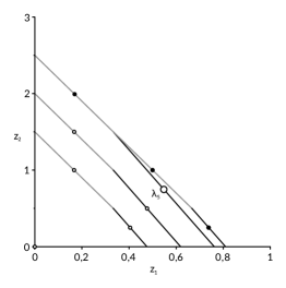
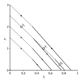
Figure 3. Constancy region associated to $\boldsymbol{\lambda}_{5}$ and $\boldsymbol{\lambda}_{6}$ (equivalently $\boldsymbol{\lambda}_{7}$ and $\boldsymbol{\lambda}_{8}$).

$\bullet$ Steps 7 and 8. The points $\boldsymbol{\lambda}_{7}:=\left(\frac{1}{2},1\right)$ and $\boldsymbol{\lambda}_{8}:=\left(\frac{31}{42},\frac{1}{4}\right)$ satisfy the equality $\mathcal{J}(\boldsymbol{\mathfrak{a}}^{\boldsymbol{\lambda}_{8}})=\mathcal{J}(\boldsymbol{\mathfrak{a}}^{\boldsymbol{\lambda}_{7}})=\mathcal{J}(\boldsymbol{\mathfrak{a}}^{\boldsymbol{\lambda}_{6}})$ so they have the same region. We update the sets $N$ and $D$ to obtain:

• $N=\{\left(\frac{1}{6},\frac{5}{2}\right)\left(\frac{13}{21},1\right)\}$.

• $D=\{\left(0,0\right),\left(\frac{1}{6},1\right),\left(\frac{17}{42},\frac{1}{4}\right),\left(\frac{1}{6},\frac{3}{2}\right),\left(\frac{10}{21},\frac{1}{2}\right),\left(\frac{23}{42},\frac{3}{4}\right),\left(\frac{1}{6},2\right),\left(\frac{1}{2},1\right),\left(\frac{31}{42},\frac{1}{4}\right)\}$.

4. Jumping divisors

The theory of jumping divisors was introduced in [1, §4] in order to describe the jump between two consecutive multiplier ideals. The aim of this section is to extend these notions to the case of mixed multiplier ideals. More importantly, the theory of jumping divisors is the right framework that provides the technical results needed in the proofs of the key results Theorem 3.3 and Proposition 3.10.

The proofs of the results that we present in this section are a straightforward extension of the ones given in [1, §4]. However, we include them for completeness. We begin with a generalization of the notion of contribution introduced by Smith and Thompson in [20] and further developed by Tucker in [21].

Definition 4.1.

Let $\boldsymbol{\mathfrak{a}}:=\left(\mathfrak{a}_{1},\ldots,\mathfrak{a}_{r}\right)\subseteq\left({\mathcal{O}}_{X,O}\right)^{r}$ be a tuple of ideals, ${\boldsymbol{\lambda}}\in\mathbb{R}_{\geqslant 0}^{r}$ a point and $G\leqslant\sum_{i=1}^{r}F_{i}$ a reduced divisor satisfying $\lambda_{1}e_{1,i}+\cdots+\lambda_{r}e_{r,i}-k_{i}\in{\mathbb{Z}}$.Then it is said that $G$ contributes to $\boldsymbol{\lambda}$ if

$$\pi_{*}\mathcal{O}_{X^{\prime}}(\lceil K_{\pi}-\lambda_{1}F_{1}-\cdots-\lambda_{r}F_{r}\rceil+G)\varsupsetneq\mathcal{J}\left({\boldsymbol{\mathfrak{a}}}^{\boldsymbol{\lambda}}\right)\,.$$

Moreover, this contribution is critical if for any divisor $0\leqslant G^{\prime}<G$ we have

$$\pi_{*}\mathcal{O}_{X^{\prime}}(\lceil K_{\pi}-\lambda_{1}F_{1}-\cdots-\lambda_{r}F_{r}\rceil+G^{\prime})=\mathcal{J}({\boldsymbol{\mathfrak{a}}}^{\boldsymbol{\lambda}}).$$

The following is the natural extension of [1, Definition 4.1] to the context of mixed multiplier ideals.

Definition 4.2.

Let ${\boldsymbol{\lambda}}:=(\lambda_{1},\dots,\lambda_{r})\in\mathbb{R}_{\geqslant 0}^{r}$ be a jumping point of a tuple of ideals $\boldsymbol{\mathfrak{a}}:=\left(\mathfrak{a}_{1},\ldots,\mathfrak{a}_{r}\right)\subseteq\left({\mathcal{O}}_{X,O}\right)^{r}$. A reduced divisor $G\leqslant\sum_{i=1}^{r}F_{i}$ for which any $E_{j}\leqslant G$ satisfies

$$\lambda_{1}e_{1,j}+\cdots+\lambda_{r}e_{r,j}-k_{j}\in{\mathbb{Z}}_{>0}$$

is called a jumping divisor for $\boldsymbol{\lambda}$ if

$$\mathcal{J}({\boldsymbol{\mathfrak{a}}}^{\boldsymbol{\lambda^{\prime}}})=\pi_{*}\mathcal{O}_{X^{\prime}}(\lceil K_{\pi}-\lambda_{1}F_{1}-\cdots-\lambda_{r}F_{r}\rceil+G)\,,$$

for any $\boldsymbol{\lambda^{\prime}}\in\{\boldsymbol{\lambda}-\mathbb{R}_{\geqslant 0}^{r}\}\cap B_{\varepsilon}(\boldsymbol{\lambda})$ for $\varepsilon$ small enough. We say that a jumping divisor is minimal if no proper subdivisor is a jumping divisor for $\boldsymbol{\lambda}$, i.e.,

$$\mathcal{J}({\boldsymbol{\mathfrak{a}}}^{\boldsymbol{\lambda^{\prime}}})\varsupsetneq\pi_{*}\mathcal{O}_{X^{\prime}}(\lceil K_{\pi}-\lambda_{1}F_{1}-\cdots-\lambda_{r}F_{r}\rceil+G^{\prime})$$

for any $0\leqslant G^{\prime}<G$ and for any $\boldsymbol{\lambda^{\prime}}\in\{\boldsymbol{\lambda}-\mathbb{R}_{\geqslant 0}^{r}\}\cap B_{\varepsilon}(\boldsymbol{\lambda})$ for $\varepsilon>0$ sufficiently small.

Among all jumping divisors we will single out the minimal jumping divisor that is constructed following closely Algorithm 3.11.

Definition 4.3.

Let $\boldsymbol{\mathfrak{a}}:=\left(\mathfrak{a}_{1},\ldots,\mathfrak{a}_{r}\right)\subseteq\left({\mathcal{O}}_{X,O}\right)^{r}$ be a tuple of ideals. Given a jumping point $\boldsymbol{\lambda}\in\mathbb{R}^{r}_{\geqslant 0}$, the corresponding minimal jumping divisor is the reduced divisor ${G_{\lambda}\leqslant\sum_{i=1}^{r}F_{i}}$ supported on those components $E_{j}$ for which the point $\boldsymbol{\lambda}$ satisfies

$$\lambda_{1}e_{1,j}+\cdots+\lambda_{r}e_{r,j}=k_{j}+1+e_{j}^{(1-\varepsilon){\boldsymbol{\lambda}}}\,,$$

where, for a sufficiently small $\varepsilon>0$, $D_{(1-\varepsilon)\boldsymbol{\lambda}}=\sum e_{j}^{(1-\varepsilon){\boldsymbol{\lambda}}}\hskip 2.84526ptE_{j}$ is the antinef closure of

$$\lfloor(1-\varepsilon){\lambda_{1}}F_{1}+\cdots+(1-\varepsilon){\lambda_{r}}F_{r}-K_{\pi}\rfloor.$$

Remark 4.4.

A jumping point $\boldsymbol{\lambda}$ is contained in some $\mathcal{C}$-facets of ${\mathcal{C}}_{\boldsymbol{\mathfrak{a}}}((1-\varepsilon)\boldsymbol{\lambda})$. The exceptional components $E_{j}$ such that $H_{j}:\hskip 2.84526pt\lambda_{1}e_{1,j}+\cdots+\lambda_{r}e_{r,j}=k_{j}+1+e_{j}^{(1-\varepsilon){\boldsymbol{\lambda}}}$ are the supporting hyperplanes of these $\mathcal{C}$-facets are precisely the components of the minimal jumping divisor $G_{\boldsymbol{\lambda}}$.

Remark 4.5.

For $\varepsilon>0$ small enough we have

$$G_{\boldsymbol{\lambda}}\leqslant\lceil K_{\pi}-(1-\varepsilon)\lambda_{1}F_{1}-\cdots-(1-\varepsilon)\lambda_{r}F_{r}\rceil-\lceil K_{\pi}-\lambda_{1}F_{1}-\cdots-\lambda_{r}F_{r}\rfloor.$$

The minimal jumping divisor is not only related to a jumping point, indeed we can associate it to the interior of each ${\mathcal{C}}$-facet.

Lemma 4.6.

The interior points of a ${\mathcal{C}}$-facet have the same minimal jumping divisor.

Proof.

This is a direct consequence of Remark 4.4. ∎

We will prove next that $G_{\boldsymbol{\lambda}}$ is a jumping divisor and deserves its name:

Proposition 4.7.

Let $\boldsymbol{\lambda}$ be a jumping point of a tuple of ideals $\boldsymbol{\mathfrak{a}}:=\left(\mathfrak{a}_{1},\ldots,\mathfrak{a}_{r}\right)\subseteq\left({\mathcal{O}}_{X,O}\right)^{r}$. Then the reduced divisor $G_{\boldsymbol{\lambda}}$ is a jumping divisor.

Proof.

Using Remark 4.5 we have

$$\lceil K_{\pi}-(1-\varepsilon)\lambda_{1}F_{1}-\cdots-(1-\varepsilon)\lambda_{r}F_{r}\rceil\geqslant\lceil K_{\pi}-\lambda_{1}F_{1}-\cdots-\lambda_{r}F_{r}\rfloor+G_{\boldsymbol{\lambda}}$$

for a sufficiently small $\varepsilon>0$ and therefore

$$\mathcal{J}({\boldsymbol{\mathfrak{a}}}^{(1-\varepsilon)\boldsymbol{\lambda}})\supseteq\pi_{*}\mathcal{O}_{X^{\prime}}(\lceil K_{\pi}-\lambda_{1}F_{1}-\cdots-\lambda_{r}F_{r}\rceil+G_{\boldsymbol{\lambda}}).$$

For the reverse inclusion, let ${D}_{(1-\varepsilon)\boldsymbol{\lambda}}=\sum e_{i}^{(1-\varepsilon)\boldsymbol{\lambda}}E_{i}$ be the antinef closure of

$$\lfloor(1-\varepsilon)\lambda_{1}F_{1}+\cdots+(1-\varepsilon)\lambda_{r}F_{r}-K_{\pi}\rfloor.$$

We want to check that $\lfloor\lambda_{1}F_{1}+\cdots+\lambda_{r}F_{r}-K_{\pi}\rfloor-G_{\boldsymbol{\lambda}}\leqslant{D}_{(1-\varepsilon)\boldsymbol{\lambda}}$. For this purpose we consider two cases.

• If $E_{i}\leqslant G_{\boldsymbol{\lambda}}$ then we have $-k_{i}+\lambda_{1}e_{1,i}+\cdots+\lambda_{r}e_{r,i}=1+e_{i}^{(1-\varepsilon)\boldsymbol{\lambda}}$. And, in particular

  $$\lfloor\lambda_{1}e_{1,i}+\cdots+\lambda_{r}e_{r,i}-k_{i}\rfloor-1=e_{i}^{(1-\varepsilon)\boldsymbol{\lambda}}\,.$$

• If $E_{i}\not\leqslant G_{\boldsymbol{\lambda}}$ then we have $-k_{i}+\lambda_{1}e_{1,i}+\cdots+\lambda_{r}e_{r,i}<1+e_{i}^{(1-\varepsilon)\boldsymbol{\lambda}}$. Thus

  $${\lfloor\lambda_{1}e_{1,i}+\cdots+\lambda_{r}e_{r,i}-k_{i}\rfloor<1+e_{i}^{(1-\varepsilon)\boldsymbol{\lambda}}}$$

  and the result follows.

∎

Theorem 4.8.

Let $\boldsymbol{\lambda}$ be a jumping point of a tuple of ideals $\boldsymbol{\mathfrak{a}}:=\left(\mathfrak{a}_{1},\ldots,\mathfrak{a}_{r}\right)\subseteq\left({\mathcal{O}}_{X,O}\right)^{r}$. Any reduced contributing divisor $G\leqslant\sum_{i=1}^{r}F_{i}$ associated to $\boldsymbol{\lambda}$ satisfies either:

• $\mathcal{J}\left({\boldsymbol{\mathfrak{a}}}^{(1-\varepsilon)\boldsymbol{\lambda}}\right)=\pi_{*}\mathcal{O}_{X^{\prime}}(\lceil K_{\pi}-\lambda_{1}F_{1}-\cdots-\lambda_{r}F_{r}\rceil+G)\varsupsetneq\mathcal{J}({\boldsymbol{\mathfrak{a}}}^{\boldsymbol{\lambda}})$ if and only if $G_{{\boldsymbol{\lambda}}}\leqslant G$, or

• $\mathcal{J}\left({\boldsymbol{\mathfrak{a}}}^{(1-\varepsilon)\boldsymbol{\lambda}}\right)\varsupsetneq\pi_{*}\mathcal{O}_{X^{\prime}}(\lceil K_{\pi}-\lambda_{1}F_{1}-\cdots-\lambda_{r}F_{r}\rceil+G)\varsupsetneq\mathcal{J}({\boldsymbol{\mathfrak{a}}}^{\boldsymbol{\lambda}})$ otherwise.

Proof.

Since $G\leqslant H_{\boldsymbol{\lambda}}$, we have

$$\lfloor(1-\varepsilon)\lambda_{1}F_{1}+\cdots+(1-\varepsilon)\lambda_{r}F_{r}-K_{\pi}\rfloor\leqslant\lfloor\lambda_{1}F_{1}+\cdots+\lambda_{r}F_{r}-K_{\pi}\rfloor-G$$

and therefore

$$\mathcal{J}({\mathfrak{a}}^{(1-\varepsilon)\boldsymbol{\lambda}})\supseteq\pi_{*}\mathcal{O}_{X^{\prime}}(\lceil K_{\pi}-\lambda_{1}F_{1}-\cdots-\lambda_{r}F_{r}\rceil+G).$$

Now assume $G_{\boldsymbol{\lambda}}\leqslant G$. Then $\lfloor\lambda_{1}F_{1}+\cdots+\lambda_{r}F_{r}-K_{\pi}\rfloor-G\leqslant\lfloor\lambda_{1}F_{1}+\cdots+\lambda_{r}F_{r}-K_{\pi}\rfloor-G_{\boldsymbol{\lambda}}$, and using the fact that $G_{\boldsymbol{\lambda}}$ is a jumping divisor we obtain the equality

$$\mathcal{J}\left({\boldsymbol{\mathfrak{a}}}^{(1-\varepsilon)\boldsymbol{\lambda}}\right)=\pi_{*}\mathcal{O}_{X^{\prime}}(\lceil K_{\pi}-\lambda_{1}F_{1}+\cdots+\lambda_{r}F_{r}\rceil+G).$$

If $G_{\boldsymbol{\lambda}}\not\leqslant G$, we may consider a component $E_{i}\leqslant G_{\boldsymbol{\lambda}}$ such that $E_{i}\not\leqslant G$. Notice that we have

$$v_{i}({D}_{(1-\varepsilon)\boldsymbol{\lambda}}) =e_{i}^{(1-\varepsilon)\boldsymbol{\lambda}}=\lambda_{1}e_{1,i}+\cdots+\lambda_{r}e_{r,i}-k_{i}-1$$

$$<\lambda_{1}e_{1,i}+\cdots+\lambda_{r}e_{r,i}-k_{i}=v_{i}(\lfloor\lambda_{1}F_{1}+\cdots+\lambda_{r}F_{r}-K_{\pi}\rfloor-G)\,,$$

where ${D}_{(1-\varepsilon)\boldsymbol{\lambda}}=\sum e_{i}^{(1-\varepsilon)\lambda}E_{i}$ is the antinef closure of $\lfloor(1-\varepsilon)\lambda_{1}F_{1}+\cdots+(1-\varepsilon)\lambda_{r}F_{r}-K_{\pi}\rfloor$. Therefore, by Corollary 3.1, we get the strict inclusion

$$\mathcal{J}({\mathfrak{a}}^{(1-\varepsilon)\boldsymbol{\lambda}})\varsupsetneq\pi_{*}\mathcal{O}_{X^{\prime}}(\lceil K_{\pi}-\lambda_{1}F_{1}-\cdots-\lambda_{r}F_{r}\rceil+G).$$

∎

From this result we deduce the unicity of the minimal jumping divisor.

Corollary 4.9.

Let $\boldsymbol{\lambda}$ be a jumping point of a tuple of ideals $\boldsymbol{\mathfrak{a}}:=\left(\mathfrak{a}_{1},\ldots,\mathfrak{a}_{r}\right)\subseteq\left({\mathcal{O}}_{X,O}\right)^{r}$. Then $G_{\boldsymbol{\lambda}}$ is the unique minimal jumping divisor associated to $\boldsymbol{\lambda}$.

The minimal jumping divisor also allows to describe the jump of mixed multiplier ideals in the other direction, although in this case we do not have minimality for the jump.

Proposition 4.10.

Let $\boldsymbol{\lambda}$ be a jumping point of a tuple of ideals $\boldsymbol{\mathfrak{a}}\subseteq({\mathcal{O}}_{X,O})^{r}$ and $D_{(1-\varepsilon)\boldsymbol{\lambda}}$ be the antinef closure of $\lfloor(1-\varepsilon)\lambda_{1}F_{1}+\cdots+(1-\varepsilon)\lambda_{r}F_{r}-K_{\pi}\rfloor$. Then we have:

• $\mathcal{J}(\boldsymbol{\mathfrak{a}}^{(1-\varepsilon)\boldsymbol{\lambda}})\varsupsetneq\pi_{*}\mathcal{O}_{X^{\prime}}(-D_{(1-\varepsilon)\boldsymbol{\lambda}}-G_{\lambda})=\mathcal{J}(\boldsymbol{\mathfrak{a}}^{\boldsymbol{\lambda}})$.

• $\mathcal{J}(\boldsymbol{\mathfrak{a}}^{(1-\varepsilon)\boldsymbol{\lambda}})\varsupsetneq\pi_{*}\mathcal{O}_{X^{\prime}}(\lceil K_{\pi}-(1-\varepsilon)\lambda_{1}F_{1}-\cdots-(1-\varepsilon)\lambda_{r}F_{r}\rceil-G_{\lambda})=\mathcal{J}(\boldsymbol{\mathfrak{a}}^{\boldsymbol{\lambda}})$

Proof.

Let $D_{\boldsymbol{\lambda}}=\sum e_{i}^{\boldsymbol{\lambda}}E_{i}$ be the antinef closure of $\lfloor\lambda_{1}F_{1}+\cdots+\lambda_{r}F_{r}-K_{\pi}\rfloor$.

i) Since $G_{\boldsymbol{\lambda}}$ is a jumping divisor we have $\lfloor\lambda_{1}F_{1}+\cdots+\lambda_{r}F_{r}-K_{\pi}\rfloor-G_{\lambda}\leqslant D_{(1-\varepsilon)\boldsymbol{\lambda}}$, and hence $\lfloor\lambda_{1}F_{1}+\cdots+\lambda_{r}F_{r}-K_{\pi}\rfloor\leqslant D_{(1-\varepsilon)\boldsymbol{\lambda}}+G_{\boldsymbol{\lambda}}$. This gives the inclusion

$$\pi_{*}\mathcal{O}_{X^{\prime}}(-D_{(1-\varepsilon)\boldsymbol{\lambda}}-G_{\boldsymbol{\lambda}})\subseteq\mathcal{J}(\boldsymbol{\mathfrak{a}}^{\boldsymbol{\lambda}}).$$

In order to check the reverse inclusion $\pi_{*}\mathcal{O}_{X^{\prime}}(-D_{(1-\varepsilon)\boldsymbol{\lambda}}-G_{\boldsymbol{\lambda}})\supseteq\mathcal{J}(\boldsymbol{\mathfrak{a}}^{\boldsymbol{\lambda}})$, it is enough, using Corollary 3.1, to prove $v_{i}(D_{(1-\varepsilon)\boldsymbol{\lambda}}+G_{\boldsymbol{\lambda}})\leqslant v_{i}(D_{\boldsymbol{\lambda}})=e_{i}^{\boldsymbol{\lambda}}$ for any component $E_{i}$. We have $e_{i}^{(1-\varepsilon)\boldsymbol{\lambda}}\leqslant e_{i}^{\boldsymbol{\lambda}}$ just because $\mathcal{J}(\boldsymbol{\mathfrak{a}}^{(1-\varepsilon)\boldsymbol{\lambda}})\varsupsetneq\mathcal{J}(\boldsymbol{\mathfrak{a}}^{\boldsymbol{\lambda}})$ and the inequality is strict when $E_{i}\leqslant G_{\boldsymbol{\lambda}}$, so the result follows.

ii) Let $D^{\prime}$ be the antinef closure of $\lfloor(1-\varepsilon)\lambda_{1}F_{1}+\cdots+(1-\varepsilon)\lambda_{r}F_{r}-K_{\pi}\rfloor+G_{\boldsymbol{\lambda}}$. Since $G_{\boldsymbol{\lambda}}\leqslant H_{\boldsymbol{\lambda}}$ we have

$$\lfloor(1-\varepsilon)\lambda_{1}F_{1}+\cdots+(1-\varepsilon)\lambda_{r}F_{r}-K_{\pi}\rfloor+G_{\boldsymbol{\lambda}}\leqslant\lfloor(1-\varepsilon)\lambda_{1}F_{1}+\cdots+(1-\varepsilon)\lambda_{r}F_{r}-K_{\pi}\rfloor\leqslant D_{\boldsymbol{\lambda}}$$

so the inclusion $\pi_{*}\mathcal{O}_{X^{\prime}}(\lceil K_{\pi}-(1-\varepsilon)\lambda_{1}F_{1}-\cdots-(1-\varepsilon)\lambda_{r}F_{r}\rceil-G_{\boldsymbol{\lambda}})\supseteq\mathcal{J}(\boldsymbol{\mathfrak{a}}^{\boldsymbol{\lambda}})$ holds. In order to prove the reverse inclusion, we will introduce an auxiliary divisor $D=\sum d_{i}E_{i}\in\Lambda$ defined as follows:

$\cdot$ $d_{i}=\lfloor(1-\varepsilon)\lambda_{1}e_{1,i}+\cdots+(1-\varepsilon)\lambda_{r}e_{r,i}-k_{i}\rfloor+1$	if $E_{i}\leqslant G_{\boldsymbol{\lambda}}$,
$\cdot$ $d_{i}=e_{i}^{(1-\varepsilon)\boldsymbol{\lambda}}$	if $E_{i}\leqslant H_{\boldsymbol{\lambda}}$ but $E_{i}\not\leqslant G_{\boldsymbol{\lambda}}$,
$\cdot$ $d_{i}=\lfloor(1-\varepsilon)\lambda_{1}e_{1,i}+\cdots+(1-\varepsilon)\lambda_{r}e_{r,i}-k_{i}\rfloor$	otherwise.

Clearly we have $\lfloor(1-\varepsilon)\lambda_{1}F_{1}+\cdots+(1-\varepsilon)\lambda_{r}F_{r}-K_{\pi}\rfloor+G_{\boldsymbol{\lambda}}\leqslant D$, but we also have $\lfloor(1-\varepsilon)\lambda_{1}F_{1}+\cdots+(1-\varepsilon)\lambda_{r}F_{r}-K_{\pi}\rfloor\leqslant D$. Indeed,

• For $E_{i}\leqslant G_{\boldsymbol{\lambda}}$ we have

  $$\lfloor\lambda_{1}e_{1,i}+\cdots+\lambda_{r}e_{r,i}-k_{i}\rfloor =\lambda_{1}e_{1,i}+\cdots+\lambda_{r}e_{r,i}-k_{i}$$

  $$=\lfloor(1-\varepsilon)\lambda_{1}e_{1,i}+\cdots+(1-\varepsilon)\lambda_{r}e_{r,i}-k_{i}\rfloor+1=d_{i}\,.$$

• If $\lambda$ is a candidate for $E_{i}$ but $E_{i}\not\leqslant G_{\boldsymbol{\lambda}}$,

  $$\lfloor\lambda_{1}e_{1,i}+\cdots+\lambda_{r}e_{r,i}-k_{i}=\lambda_{1}e_{1,i}+\cdots+\lambda_{r}e_{r,i}-k_{i}<1+e_{i}^{(1-\varepsilon)\boldsymbol{\lambda}}\,,$$

  hence $\lfloor\lambda_{1}e_{1,i}+\cdots+\lambda_{r}e_{r,i}-k_{i}\rfloor\leqslant e_{i}^{(1-\varepsilon)\boldsymbol{\lambda}}=d_{i}\,.$

• Otherwise

  $$\lfloor\lambda_{1}e_{1,i}+\cdots+\lambda_{r}e_{r,i}-k_{i}\rfloor=\lfloor(1-\varepsilon)\lambda_{1}e_{1,i}+\cdots+(1-\varepsilon)\lambda_{r}e_{r,i}-k_{i}\rfloor=d_{i}\,.$$

Therefore, taking antinef closures, we have $D^{\prime}\leqslant D_{\boldsymbol{\lambda}}\leqslant\widetilde{D}$. On the other hand $D\leqslant D^{\prime}$. Namely, $v_{i}(D^{\prime})\geqslant e_{i}^{(1-\varepsilon)\boldsymbol{\lambda}}$ at any $E_{i}$ because

$$\lfloor(1-\varepsilon)\lambda_{1}F_{1}+\cdots+(1-\varepsilon)\lambda_{r}F_{r}-K_{\pi}\rfloor\leqslant\lfloor(1-\varepsilon)\lambda_{1}F_{1}+\cdots+(1-\varepsilon)\lambda_{r}F_{r}-K_{\pi}\rfloor+G_{\boldsymbol{\lambda}}\,.$$

Moreover, $v_{i}(D^{\prime})\geqslant\lfloor(1-\varepsilon)\lambda_{1}e_{1,i}+\cdots+(1-\varepsilon)\lambda_{r}e_{r,i}-k_{i}\rfloor+\delta_{i}^{G_{\boldsymbol{\lambda}}}$ by definition of antinef closure. Here, $\delta_{i}^{G_{\boldsymbol{\lambda}}}=1$ if $E_{i}\leqslant G_{\boldsymbol{\lambda}}$ and zero otherwise. Thus $v_{i}(D^{\prime})\geqslant v_{i}(D)$ as desired. As a consequence $\widetilde{D}\leqslant D^{\prime}$, which, together with the previous $D^{\prime}\leqslant D_{\boldsymbol{\lambda}}\leqslant\widetilde{D}$, gives $\widetilde{D}=D^{\prime}=D_{\boldsymbol{\lambda}}$ and the result follows. ∎

4.1. Geometric properties of minimal jumping divisors in the dual graph

We proved in [1, Theorem 4.17] that minimal jumping divisors associated to satisfy some geometric conditions in the dual graph in the case of multiplier ideals. The same properties hold for mixed multiplier ideals. More interestingly, the forthcoming Theorem 4.14 is the key result that we need in the proof of Theorem 3.3.

Lemma 4.11.

Let $\boldsymbol{\lambda}$ be a jumping point of a tuple of ideals $\boldsymbol{\mathfrak{a}}:=\left(\mathfrak{a}_{1},\ldots,\mathfrak{a}_{r}\right)\subseteq\left({\mathcal{O}}_{X,O}\right)^{r}$. For any component $E_{i}\leqslant G_{\boldsymbol{\lambda}}$ of the minimal jumping divisor $G_{\boldsymbol{\lambda}}$ we have:

$$\left(\left\lceil K_{\pi}-\lambda_{1}F_{1}-\cdots-\lambda_{r}F_{r}\right\rceil+G_{\boldsymbol{\lambda}}\right)\cdot E_{i}\\ =-2+\lambda_{1}\rho_{1,i}+\cdots+\lambda_{r}\rho_{r,i}+a_{G_{\boldsymbol{\lambda}}}\left(E_{i}\right)+\sum_{E_{j}\in\mathrm{Adj}(E_{i})}\left\{\lambda_{1}e_{1,j}+\cdots+\lambda_{r}e_{r,j}-k_{j}\right\}\,.$$

where $\mathrm{Adj}(E_{i})$ denotes the adjacent components of $E_{i}$ in the dual graph.

Proof.

For any $E_{i}\leqslant G_{\boldsymbol{\lambda}}$ we have:

$(\left\lceil K_{\pi}-\lambda_{1}F_{1}-\cdots-\lambda_{r}F_{r}\right\rceil+G_{\boldsymbol{\lambda}})\cdot E_{i}$

$\hskip 14.22636pt=(\left(K_{\pi}-\lambda_{1}F_{1}-\cdots-\lambda_{r}F_{r}\right)+\left\{-K_{\pi}+\lambda_{1}F_{1}+\cdots+\lambda_{r}F_{r}\right\}+G_{\boldsymbol{\lambda}}-E_{i}+E_{i})\cdot E_{i}$

$\hskip 14.22636pt=\left(K_{\pi}+E_{i}\right)\cdot E_{i}-(\lambda_{1}F_{1}+\cdots+\lambda_{r}F_{r})\cdot E_{i}+\left\{\lambda_{1}F_{1}+\cdots+\lambda_{r}F_{r}-K_{\pi}\right\}\cdot E_{i}+\left(G_{\boldsymbol{\lambda}}-E_{i}\right)\cdot E_{i}.$

Let us now compute each summand separately. Firstly, the adjunction formula gives $\left(K_{\pi}+E_{i}\right)\cdot E_{i}=-2$ because $E_{i}\cong{\mathbb{P}}^{1}$. As for the second and fourth terms, the equality $-(\lambda_{1}F_{1}+\cdots+\lambda_{r}F_{r})\cdot E_{i}=\lambda_{1}\rho_{1,i}+\cdots+\lambda_{r}\rho_{r,i}$ follows from the definition of the excesses, and clearly $a_{G_{\boldsymbol{\lambda}}}\left(E_{i}\right)=\left(G_{\boldsymbol{\lambda}}-E_{i}\right)\cdot E_{i}$ because $E_{i}\leqslant G_{\boldsymbol{\lambda}}$. Therefore it only remains to prove that

(4.1) $$\left\{\lambda_{1}F_{1}+\cdots+\lambda_{r}F_{r}-K_{\pi}\right\}\cdot E_{i}=\sum_{E_{j}\in\mathrm{Adj}(E_{i})}\left\{\lambda_{1}e_{1,j}+\cdots+\lambda_{r}e_{r,j}-k_{j}\right\},$$

which is also quite immediate. Indeed, writing

$$\left\{\lambda_{1}F_{1}+\cdots+\lambda_{r}F_{r}-K_{\pi}\right\}=\sum_{j=1}^{\ell}\left\{\lambda_{1}e_{1,j}+\cdots+\lambda_{r}e_{r,j}-k_{j}\right\}E_{j}\,,$$

equality (4.1) follows by observing that (for $j\neq i$), $E_{j}\cdot E_{i}=1$ if and only if $E_{j}\in\mathrm{Adj}\left(E_{i}\right)$, and the term corresponding to $j=i$ vanishes because we have ${\lambda_{1}e_{1,i}+\cdots+\lambda_{r}e_{r,i}-k_{i}\in{\mathbb{Z}}}$. ∎

Corollary 4.12.

Let $\boldsymbol{\lambda}$ be a jumping point of a tuple of ideals $\boldsymbol{\mathfrak{a}}\subseteq\left({\mathcal{O}}_{X,O}\right)^{r}$. For any component $E_{i}\leqslant G_{\boldsymbol{\lambda}}$ of the minimal jumping divisor $G_{\boldsymbol{\lambda}}$ we have:

$$\lambda_{1}\rho_{1,i}+\cdots+\lambda_{r}\rho_{r,i}+a_{G_{\boldsymbol{\lambda}}}\left(E_{i}\right)+\sum_{E_{j}\in\mathrm{Adj}(E_{i})}\left\{\lambda_{1}e_{1,j}+\cdots+\lambda_{r}e_{r,j}-k_{j}\right\}\in\mathbb{Z}$$

As in the case of multiplier ideals, minimal jumping divisors satisfy a nice numerical condition.

Proposition 4.13.

Let $\boldsymbol{\lambda}$ be a jumping point of a tuple of ideals $\boldsymbol{\mathfrak{a}}\subseteq\left({\mathcal{O}}_{X,O}\right)^{r}$. For any component $E_{i}\leqslant G_{\boldsymbol{\lambda}}$ of the minimal jumping divisor $G_{\boldsymbol{\lambda}}$, we have

$$\left(\left\lceil K_{\pi}-\lambda_{1}F_{1}-\cdots-\lambda_{r}F_{r}\right\rceil+G_{\boldsymbol{\lambda}}\right)\cdot E_{i}\geqslant 0.$$

Proof.

Given a prime divisor $E_{i}\leqslant G_{\boldsymbol{\lambda}}$, we consider the short exact sequence

$$0\longrightarrow\mathcal{O}_{X^{\prime}}\left(\left\lceil K_{\pi}-\lambda_{1}F_{1}-\cdots-\lambda_{r}F_{r}\right\rceil+G_{\boldsymbol{\lambda}}-E_{i}\right)\longrightarrow$$

$$\qquad\longrightarrow\mathcal{O}_{X^{\prime}}\left(\left\lceil K_{\pi}-\lambda_{1}F_{1}-\cdots-\lambda_{r}F_{r}\right\rceil+G_{\boldsymbol{\lambda}}\right)\longrightarrow$$

$$\qquad\qquad\longrightarrow\mathcal{O}_{E_{i}}\left(\left\lceil K_{\pi}-\lambda_{1}F_{1}-\cdots-\lambda_{r}F_{r}\right\rceil+G_{\boldsymbol{\lambda}}\right)\longrightarrow 0$$

Pushing it forward to $X$, we get

$$0\longrightarrow\pi_{*}\mathcal{O}_{X^{\prime}}\left(\left\lceil K_{\pi}-\lambda_{1}F_{1}-\cdots-\lambda_{r}F_{r}\right\rceil+G_{\boldsymbol{\lambda}}-E_{i}\right)\longrightarrow$$

$$\qquad\longrightarrow\pi_{*}\mathcal{O}_{X^{\prime}}\left(\left\lceil K_{\pi}-\lambda_{1}F_{1}-\cdots-\lambda_{r}F_{r}\right\rceil+G_{\boldsymbol{\lambda}}\right)\longrightarrow$$

$$\qquad\qquad\longrightarrow H^{0}\left(E_{i},\mathcal{O}_{E_{i}}\left(\left\lceil K_{\pi}-\lambda_{1}F_{1}-\cdots-\lambda_{r}F_{r}\right\rceil+G_{\lambda}\right)\right)\otimes\mathbb{C}_{O},$$

where $\mathbb{C}_{O}$ denotes the skyscraper sheaf supported at $O$ with fibre $\mathbb{C}$. The minimality of $G_{\boldsymbol{\lambda}}$ (see Corollary 4.9) implies that

$$\pi_{*}\mathcal{O}_{X^{\prime}}\left(\left\lceil K_{\pi}-\lambda_{1}F_{1}-\cdots-\lambda_{r}F_{r}\right\rceil+G_{\boldsymbol{\lambda}}-E_{i}\right)\neq\pi_{*}\mathcal{O}_{X^{\prime}}\left(\left\lceil K_{\pi}-\lambda_{1}F_{1}-\cdots-\lambda_{r}F_{r}\right\rceil+G_{\boldsymbol{\lambda}}\right).$$

Thus $H^{0}\left(E_{i},\mathcal{O}_{E_{i}}\left(\left\lceil K_{\pi}-\lambda_{1}F_{1}-\cdots-\lambda_{r}F_{r}\right\rceil+G_{\boldsymbol{\lambda}}\right)\right)\neq 0$, or equivalently

$$\left(\left\lceil K_{\pi}-\lambda_{1}F_{1}-\cdots-\lambda_{r}F_{r}\right\rceil+G_{\boldsymbol{\lambda}}\right)\cdot E_{i}\geqslant 0.$$

∎

With the above ingredients we can provide the desired geometric property of the minimal jumping divisors when viewed in the dual graph.

Theorem 4.14.

Let $G_{\boldsymbol{\lambda}}$ be the minimal jumping divisor associated to a jumping point $\boldsymbol{\lambda}$ of a tuple of ideals $\boldsymbol{\mathfrak{a}}\subseteq\left({\mathcal{O}}_{X,O}\right)^{r}$. Then the ends of a connected component of $G_{\boldsymbol{\lambda}}$ must be either rupture or dicritical divisors.

Proof.

Assume that an end $E_{i}$ of a connected component of $G_{\boldsymbol{\lambda}}$ is neither a rupture nor a dicritical divisor. It means that $E_{i}$ has no excess, i.e., $\rho_{j,i}=0$ for all $E_{j}$ of the resolution, and that it has one or two adjacent divisors, say $E_{j}$ and $E_{l}$, in the dual graph but at most one of them belongs to $G_{\boldsymbol{\lambda}}$.

For the case that $E_{i}$ has two adjacent divisors $E_{j}$ and $E_{l}$, the formula given in Lemma 4.11 reduces to

$$(\lceil K_{\pi}-\lambda_{1}F_{1}-\cdots-\lambda_{r}F_{r}\rceil+G_{\boldsymbol{\lambda}})\cdot E_{i}$$

$$\qquad=-2+\left\{\lambda_{1}e_{1,j}+\cdots+\lambda_{r}e_{r,j}-k_{j}\right\}+\left\{\lambda_{1}e_{1,l}+\cdots+\lambda_{r}e_{r,l}-k_{l}\right\}$$

$$\qquad\qquad+\lambda_{1}\rho_{1,i}+\cdots+\lambda_{r}\rho_{r,i}+a_{G_{\boldsymbol{\lambda}}}(E_{i})\,.$$

Then:

• If $E_{i}$ has valence one in $G_{\boldsymbol{\lambda}}$, e.g. $E_{l}\not\leqslant G_{\boldsymbol{\lambda}}$, then

  $$(\lceil K_{\pi}-\lambda_{1}F_{1}-\cdots-\lambda_{r}F_{r}\rceil+G_{\boldsymbol{\lambda}})\cdot E_{i}=-2+\left\{\lambda_{1}e_{1,l}+\cdots+\lambda_{r}e_{r,l}-k_{l}\right\}+1<0\,.$$

• If $E_{i}$ is an isolated component of $G_{\boldsymbol{\lambda}}$, i.e., $E_{j},E_{l}\not\leqslant G_{\boldsymbol{\lambda}}$, then

  $$(\lceil K_{\pi}-\lambda_{1}F_{1}-\cdots-\lambda_{r}F_{r}\rceil+G_{\boldsymbol{\lambda}})\cdot E_{i}$$

  $$\qquad=-2+\left\{\lambda_{1}e_{1,j}+\cdots+\lambda_{r}e_{r,j}-k_{j}\right\}+\left\{\lambda_{1}e_{1,l}+\cdots+\lambda_{r}e_{r,l}-k_{l}\right\}<0.$$

If $E_{i}$ has just one adjacent divisor $E_{j}$, i.e. $E_{i}$ is an end of the dual graph, the formula reduces to

$$(\lceil K_{\pi}-\lambda_{1}F_{1}-\cdots-\lambda_{r}F_{r}\rceil+G_{\boldsymbol{\lambda}})\cdot E_{i}$$

$$\qquad=-2+\left\{\lambda_{1}e_{1,j}+\cdots+\lambda_{r}e_{r,j}-k_{j}\right\}+\lambda_{1}\rho_{1,i}+\cdots+\lambda_{r}\rho_{r,i}+a_{G_{\boldsymbol{\lambda}}}(E_{i})\,.$$

Therefore,

• If $E_{i}$ has valence one in $G_{\boldsymbol{\lambda}}$, then

  $$(\lceil K_{\pi}-\lambda_{1}F_{1}-\cdots-\lambda_{r}F_{r}\rceil+G_{\boldsymbol{\lambda}})\cdot E_{i}=-2+1<0\,.$$

• If $E_{i}$ is an isolated component of $G_{\boldsymbol{\lambda}}$, then

  $$(\lceil K_{\pi}-\lambda_{1}F_{1}-\cdots-\lambda_{r}F_{r}\rceil+G_{\boldsymbol{\lambda}})\cdot E_{i}=-2+\left\{\lambda_{1}e_{1,j}+\cdots+\lambda_{r}e_{r,j}-k_{j}\right\}<0.$$

In any case we get a contradiction with Proposition 4.13. ∎

As a consequence of this result we can also provide the following refinement of Proposition 4.13.

Proposition 4.15.

Let $\boldsymbol{\lambda}$ be a jumping point of a tuple of ideals $\boldsymbol{\mathfrak{a}}\subseteq\left({\mathcal{O}}_{X,O}\right)^{r}$. If $E_{i}\leqslant G_{\boldsymbol{\lambda}}$ is neither a rupture nor a dicritical component of the minimal jumping divisor $G_{\boldsymbol{\lambda}}$ we have

$$\left(\left\lceil K_{\pi}-\lambda_{1}F_{1}-\cdots-\lambda_{r}F_{r}\right\rceil+G_{\boldsymbol{\lambda}}\right)\cdot E_{i}=0.$$

Proof.

Assume that $E_{i}\leqslant G_{\boldsymbol{\lambda}}$ is neither a rupture or a dicritical component. In particular, it is not the end of a connected component of $G_{\boldsymbol{\lambda}}$. Thus, $E_{i}$ has exactly two adjacent components $E_{j}$ and $E_{l}$ in $G_{\boldsymbol{\lambda}}$, and its excesses are $\rho_{j,i}=0$ for all $1\leqslant j\leqslant r$. The formula given in Lemma 4.11 for $G_{\boldsymbol{\lambda}}$ reduces to

$$\left(\left\lceil K_{\pi}-\lambda_{1}F_{1}-\cdots-\lambda_{r}F_{r}\right\rceil+G_{\boldsymbol{\lambda}}\right)\cdot E_{i}$$

$$\qquad=-2+\lambda_{1}\rho_{1,i}+\cdots+\lambda_{r}\rho_{r,i}+\left\{\lambda_{1}e_{1,j}+\cdots+\lambda_{r}e_{r,j}-k_{j}\right\}$$

$$\qquad\qquad{}+\left\{\lambda_{1}e_{1,l}+\cdots+\lambda_{r}e_{r,l}-k_{l}\right\}+a_{G_{\lambda}}\left(E_{i}\right)\,.$$

Notice that $a_{G_{\boldsymbol{\lambda}}}(E_{i})=2$, and also that

$$\left\{\lambda_{1}e_{1,j}+\cdots+\lambda_{r}e_{r,j}-k_{j}\right\}=\left\{\lambda_{1}e_{1,l}+\cdots+\lambda_{r}e_{r,l}-k_{l}\right\}=0\,,$$

because $E_{j}$ and $E_{l}$ are components of $G_{\lambda}$, so finally

$$\left(\left\lceil K_{\pi}-\lambda_{1}F_{1}-\cdots-\lambda_{r}F_{r}\right\rceil+G_{\boldsymbol{\lambda}}\right)\cdot E_{i}=0\,.$$

∎

References

- [1] M. Alberich-Carramiñana, J.Àlvarez Montaner and F. Dachs-Cadefau, Multiplier ideals in two-dimensional local rings with rational singularities, preprint available at arXiv:1412.3605. To appear in Mich. Math. J.
- [2] M. Alberich-Carramiñana, J.Àlvarez Montaner, F. Dachs-Cadefau and V. González-Alonso, Poincaré series of multiplier ideals in two-dimensional local rings with rational singularities, preprint available at arXiv:1412.3607.
- [3] M. Artin, On isolated rational singularities of surfaces, Amer. J. Math. 68 (1966), 129–136.
- [4] E. Casas-Alvero, Singularities of plane curves, London Math. Soc. Lecture Note Series, 276, Cambridge University Press, Cambridge, 2000.
- [5] Pi. Cassou-Noguès and A. Libgober, Multivariable Hodge theoretical invariants of germs of plane curves, J. Knot Theory Ramifications 20 (2011), 787–805.
- [6] Pi. Cassou-Noguès and A. Libgober, Multivariable Hodge theoretical invariants of germs of plane curves II, in Valuation Theory in Interaction. Eds. A Campillo, F.-V. Kuhlmann and B. Teissier. EMS Series of Congress Reports 10 (2014), 82–135.
- [7] F. Dachs-Cadefau, Multiplier ideals in two-dimensional local rings with rational singularities, Ph.D. Thesis, KU Leuven and Universitat Politècnica de Catalunya, 2016.
- [8] L. Ein, R. Lazarsfeld, K. Smith and D. Varolin, Jumping coefficients of multiplier ideals, Duke Math. J. 123 (2004), 469–506.
- [9] F. Enriques and O. Chisini, Lezioni sulla teoria geometrica delle equazioni e delle funzioni algebriche, N. Zanichelli, Bologna, (1915).
- [10] T. Järviletho, Jumping numbers of a simple complete ideal in a two-dimensional regular local ring, Mem. Amer. Math. Soc. 214 (2011), no. 1009, viii+78 pp.
- [11] H. Laufer, On rational singularities, Amer. J. Math. 94 (1972), 597–608.
- [12] R. Lazarsfeld, Positivity in algebraic geometry. II, volume 49, (2004), Springer-Verlag, xviii+385.
- [13] A. Libgober, Hodge decomposition of Alexander invariants, Manuscripta Math. 107 (2002) 251–269.
- [14] A. Libgober and M. Mustaţă, Sequences of LCT-polytopes, Math. Res. Lett. 18 (2011) 733–746.
- [15] J. Lipman, Rational singularities, with applications to algebraic surfaces and unique factorization, Inst. Hautes tudes Sci. Publ. Math. 36 (1969) 195–279.
- [16] D. Naie, Jumping numbers of a unibranch curve on a smooth surface, Manuscripta Math. 128 (2009), 33–49.
- [17] D. Naie, Mixed multiplier ideals and the irregularity of abelian coverings of smooth projective surfaces, Expo. Math. 31 (2013), 40–72.
- [18] F. Pérez, On the constancy regions for mixed test ideals, J. Algebra 396 (2013), 82–97.
- [19] A. J. Reguera, Curves and proximity on rational surface singularities, J. Pure Appl. Algebra 122 (1997) 107–126.
- [20] K. E. Smith and H. Thompson, Irrelevant exceptional divisors for curves on a smooth surface. in: Algebra, geometry and their interactions, Contemp. Math. 448 (2007), 245–254.
- [21] K. Tucker, Jumping numbers on algebraic surfaces with rational singularities, Trans. Amer. Math. Soc. 362 (2010), 3223–3241.