Shape minimization problems in liquid crystals

Abstract

We consider a class of liquid crystal free-boundary problems for which both the equilibrium shape and internal configuration of a system must simultaneously be determined, for example in films with air- or fluid-liquid crystal interfaces and elastomers. We develop a finite element algorithm to solve such problems with dynamic mesh control, achieved by supplementing the free energy with an auxiliary functional that promotes mesh quality and is minimized in the null space of the energy. We apply this algorithm to a flexible capacitor, as well as to determine the shape of liquid crystal tactoids as a function of the surface tension and elastic constants. These are compared with theoretical predictions and experimental observations of tactoids from the literature.

I Introduction

Surface effects are of fundamental importance in liquid crystal physicsBarbero and Evangelista (2005); Rasing and Musevic (2013). Chemical and topographical treatments induce a preferred molecular orientation that, due to elasticity, tends to align the material in the bulk. Patterned surfaces produce a wealth of phenomena, including multistable alignmentKim et al. (2002); Atherton and Adler (2012) and arbitrary control of the alignment orientation and associated anchoring energyKondrat et al. (2005); Anquetil-Deck et al. (2013). Highly confined liquid crystals, in channels, emulsion droplets, or polymer dispersed systems are also strongly influenced by the interaction of the LC material with the adjacent medium. As liquid crystals are deployed beyond display applicationsLagerwall and Scalia (2012), the exploration of their behavior in complex geometries has become increasingly important. Almost ubiquitously, the shape of their enclosure is regarded as a rigid body and the equilibrium configuration of the liquid crystal found by minimizing an appropriate energy functional, a challenging enough task given the multiple competing physical effects—elasticity, surfaces, applied and internal fields—involved. If the external environment is not rigid, the minimization problem also requires solving for the shape of the body. It is this latter category that shall be discussed in this paper, which we refer to as shape-order problems since they require simultaneous solution of both shape and ordering.

One situation where the variable shape problem may occur is when droplets or shells of liquid crystalline phase are dispersed in an isotropic fluid. For thermotropic liquid crystals, the nematic-isotropic interfacial energy is much larger than the elastic energy, and such droplets remain approximately spherical. Topology restricts the number and type of defects on the surfaceMacKintosh and Lubensky (1991); Fernández-Nieves et al. (2007), which can be used to template other objects Whitmer et al. (2013). For lyotropic materials, however, the effective energy of the phase boundary is weak and highly deformed droplets, known as tactoids, are observed. Observed in dilute vanadium pentoxide by Zocher Zocher (1925); Zocher and Jacobsohn (1929) in 1925 and assemblies of viral particles Bernal and Fankuchen Bernal and Fankuchen (1941) in 1941, there has been a resurgence of interest in the last couple of decades and a rich variety of morphologies observed. In an applied electric field, paramagnetic tactoids are deformed strongly as a flow field develops internally Sonin (1998). While most tactoids observed possess a characteristic eye shape, a rare triangular version has been seen using an actin system with crosslinkers Tang et al. (2005). Non simply-connected shapes are commonly seen, with the isotropic inclusions themselves forming negative tactoids Casagrande et al. (1987) and examples with many inclusions and defects have been seen in chromonic liquid crystals Kim et al. (2013). While for most tactoids the anchoring is parallel to the interface, elongation has also been seen in small droplets with perpendicular (homeotropic) anchoring Verhoeff et al. (2011). Tactoid structures have been shown to act as sensors via chirality amplification Peng and Lavrentovich (2015) and can be used to guide motile bacteria Mushenheim et al. (2014); Zhou et al. (2014). They are also valuable architectural elements of self assembly, for example providing nucleation sites for growth of the smectic phase Dogic and Fraden (2001).

Theoretical treatments of tactoids are more sparse due to the difficulty of the combined shape-order minimization problem. Chandrasekhar argued for a taxonomy of four possible shapes Chandrasekhar (1966): elliptical, rectangular, a rounded rectangle and the eye shape observed in earlier experimental work. Kaznacheev proposed an elastic theory Kaznacheev et al. (2003) for the size-dependence of the equilibrium shape, determining that larger tactoids become more spherical in agreement with experiments Kaznacheev et al. (2002). Prinsen argued that the aspect ratio of the tactoid depends primarily on the anchoring strength while the configuration of the director field depends on the ratio of anchoring to elastic constant Prinsen and van der Schoot (2003). In a second paper, they showed that differences between elastic constants can lead to several different stable director configurations and predicted a phase diagram for the ground state Prinsen and Van Der Schoot (2004). Simulation based approaches have been used to study tactoids. Bates used a Monte Carlo approach to show the tendency of droplets to elongate Bates (2003). Recently, a coarse grained simulation Vanzo et al. (2012) of $50-100nm$ droplets showed that the liquid crystal may spontaneously undergo a symmetry breaking transition to a chiral configuration in a tactoid, despite being composed of achiral materials.

A second class of materials that undergo dramatic shape change are Liquid Crystal Elastomers (LCEs), soft polymeric materials consisting of a cross-linked network and rod-like mesogens that spontaneously align. These materials combine the properties of rubbery materials and liquid crystals Warner and Terentjev (2003a). Their chief distinctive feature is the coupling between strain and orientation order: stretching a LCE material can rotate the mesogens and vice versa De Gennes (1975); Kundler and Finkelmann (1995); Finkelmann et al. (2001); Conti et al. (2002); Mbanga et al. (2010a). They may be induced to undergo large deformations by external stimuli Finkelmann et al. (2001) including electric fields Chang et al. (1997); Burridge et al. (2006); Menzel and Brand (2007); Ye et al. (2007), induced swelling by absorption of solvent molecules Urayama et al. (2003, 2006) and light Yu et al. (2003); Li et al. (2003); Camacho-Lopez et al. (2004); He (2007); Sawa et al. (2010); Mahimwalla et al. (2012). These fascinating properties suggest many applications requiring flexibility or a large response to a modest stimulus, such as soft actuators, artificial muscles, self-folding structures, smart materials, flexible displays, and flexible microgenerators Yu et al. (2002); Warner and Terentjev (2003b); Palfffy-Muhoray (2009); Xie and Zhang (2005). In light of the strong contemporary interest in these materials, some groups have begun to produce high quality numerical solvers to simulate their behaviorMbanga et al. (2010b); de Haan et al. (2014).

In light of the above applications in liquid crystal physics, as well as others in soft matter more broadly, there is a need for generic tools to solve shape-order problems. Excellent tools for shape minimization problems, such as the Surface EvolverBrakke (1992), exist but are limited to systems without order and to problems involving low dimensional manifolds. Unfortunately, these extensions make the problem much more challenging because the numerical representation—i.e. the mesh for a finite element approach—must be co-evolved during the minimization along with the boundary. In this paper, we discuss some initial explorations and propose a regularization scheme to address these difficulties. The paper is structured as follows: in section II the numerical challenges in this class of problem are discussed and a regularization strategy proposed. In section III we apply this algorithm to two problems of increasing difficulty: in subsection III.1 a flexible capacitor for which an analytical solution is available and in subsection III.2 liquid crystal tactoids. Conclusions and prospects for future work are presented in section IV.

II Regularizing Shape Minimization Problems

As an illustration of the challenges associated with shape minimization problems, consider perhaps the simplest possible example: minimize the length of a loop subject to a constant enclosed area of unity. The problem may be solved in discrete form by defining linear elements between adjacent points $\mathbf{x}_{i}$ with $i\in[1,N]$ and imposing a periodic condition $i+N\equiv i$. The program is then,

$$\min \sum_{i=1}^{N}\left\|\mathbf{x}_{i+1}-\mathbf{x}_{i}\right\|$$

s.t. $$\ \frac{1}{2}\sum_{i=1}^{N}\left\|\mathbf{x}_{i}\times(\mathbf{x}_{i+1}-\mathbf{x}_{i})\right\| =1.$$ (1)

By differentiating the target and constraint functionals, we obtain generalized forces $\mathbf{F}_{i}^{L}$ and $\mathbf{F}_{i}^{A}$ representing the generalized force on vertex $i$ exerted by the length functional and area constraint respectively. From an initial configuration $\mathbf{x}^{0}$, the program (1) is solved by taking gradient descent steps,

$$\mathbf{x}^{n+1}=\mathbf{x}^{n}+\lambda\left(\mathbf{F}^{L}-\frac{\mathbf{F}^{L}\cdot\mathbf{F}^{A}}{\mathbf{F}^{A}\cdot\mathbf{F}^{A}}\mathbf{F}^{A}\right),$$ (2)

where the component of $\mathbf{F}^{L}$ that tends to change the area is subtracted off. The stepsize $\lambda$ is determined by a line search, i.e. performing a 1D minimization of the energy functional with respect to $\lambda$. After each step, the solution is rescaled to have unit area. Although simple, this algorithm is at the core of programs like Surface Evolver whose complexity arises from the wide variety of energy functionals available. To obtain a solution, the user performs a succession of relaxation steps from an initial guess to find a solution and is able to interactively refine the mesh.

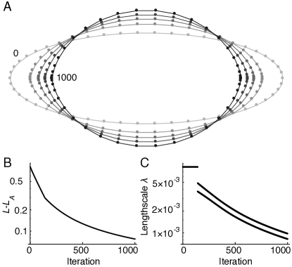
Figure 1: Minimization of the length of a loop at constant area. A Intermediate steps at iterations $0$, $100$, $200$, $400$ and $1000$. B Length of the line minus the analytical perimeter $L_{A}$ as a function of iteration. C Stepsize determined from linesearches as a function of iteration.

If the initial guess is far from the solution, however, problems can occur. In fig. 1 we display a minimization starting from an initial elliptical loop of aspect ratio $3$ and unit area. The solution converges toward the correct circular solution, but very slowly. In fig. 1A, note that mesh points that started at the ends of the ellipse become bunched together. Hence, even after $1000$ iterations, only a relatively poor approximant to the circle has been found. In fig. 1B the quantity $L-L_{A}$ is reported on log-linear scales as a function of iteration number, where $L$ is the length of the loop and $L_{A}=2\sqrt{\pi}$ is the analytical perimeter of a circle with unit area. For a good initial guess, this quantity should converge exponentially, i.e. $L-L_{A}\propto\exp\left(-kn\right)$ with some rate $k$ and hence would appear on this plot as a straight line; the line observed shows that the convergence is subexponential. The reason for this is apparent from a plot of the stepsize $\lambda$ as a function of iteration, shown in fig. 1C, that shows that the algorithm is forced to take smaller and smaller steps as the points become bunched together.

Bunching arises because the solution of the program (1) possesses a null space with respect to the position of the vertices. Suppose all vertices other than $\mathbf{x}_{i}$ are fixed, but the $i$th vertex is perturbed $\mathbf{x}_{i}\to\mathbf{x}_{i}+\mathbf{\delta}\mathbf{m}$ where $\mathbf{m}$ is a unit vector. Expanding the length of a loop as a series in $\delta$ we obtain,

$$L=L_{0}+\delta\mathbf{m}\cdot\left(\frac{\mathbf{x}_{i+1}-\mathbf{x}_{i}}{\left|\mathbf{x}_{i+1}-\mathbf{x}_{i}\right|}-\frac{\mathbf{x}_{i}-\mathbf{x}_{i-1}}{\left|\mathbf{x}_{i}-\mathbf{x}_{i-1}\right|}\right)+\cdots.$$ (3)

The change in length can be cancelled to linear order if the direction of the perturbation is chosen to be perpendicular to the second factor in the dot product. The factor in question is, by definition, the generalized force acting on the vertex $i$. At equilibrium, this must balance the force due to the area constraint, which always points along the normal. Hence, for the solution of (1), the nullspace lies for each vertex locally along the tangent line.

The existence of the nullspace reveals that the problem is underconstrained, and this characteristic is generic for shape evolution problems. For instance, if the interior of the loop were to be meshed as well, the position of these additional mesh points does not enter the program (1), and so they would not be moved. Moreover, it is an issue fundamentally associated with the discrete system as the continuous functional possesses a unique solution.

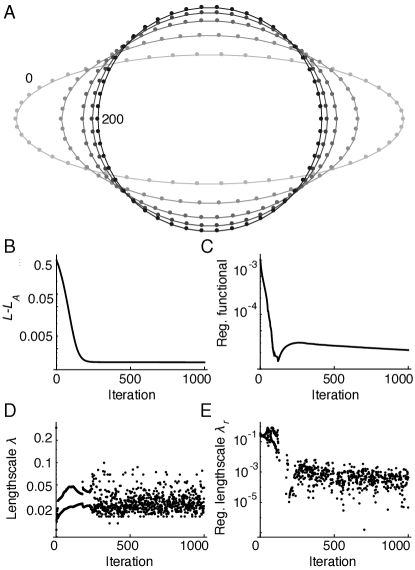
Figure 2: Minimization of the length of a loop with regularization. A Intermediate steps at iterations $0$, $40$, $80$, $120$ and $200$. B Length of the line minus the analytical perimeter $L_{A}$ as a function of iteration. C Value of the regularization functional as a function of iteration. D Stepsize $\lambda$ and E Regularization stepsize $\lambda_{r}$ as determined from linesearches by iteration.

To solve this problem, Surface Evolver permits the user to merge nearby mesh points as they become bunched, and to create new mesh points by splitting long elements. This is effective, but means that the number of mesh points cannot be controlled as easily and requires discrete changes to the mesh. Here, we propose a different solution that allows continuous regularization of the mesh. The idea is to supplement the minimization problem with an auxiliary functional that captures our intuition of mesh quality. For the present problem, a suitable functional is,

$$E_{R}=\frac{1}{2}\sum_{i}\left[\left(\left|\mathbf{x}_{i}-\mathbf{x}_{i-1}\right|-\bar{L_{i}}\right)^{2}+\left(\left|\mathbf{x}_{i+1}-\mathbf{x}_{i}\right|-\bar{L_{i}}\right)^{2}\right]$$ (4)

where $\bar{L_{i}}=\frac{1}{2}\left(\left|\mathbf{x}_{i}-\mathbf{x}_{i-1}\right|+\left|\mathbf{x}_{i+1}-\mathbf{x}_{i}\right|\right)$, i.e. the mean length of the two linear elements at point $i$. This functional favors equally spaced mesh points. By differentiating the regularization functional, a corresponding generalized force $\mathbf{F}^{R}$ may be obtained.

It is essential that the regularization functional does not interfere with the solution of the program (1), so the regularization functional is minimized separately in the nullspace of the target functional, i.e ensuring that $\mathbf{F}^{L}\cdot\mathbf{F}^{R}=\mathbf{F}^{A}\cdot\mathbf{F}^{R}=0$. Following each gradient descent step eq. (2), a regularization step is then taken,

$$\mathbf{x}^{n+1}=\mathbf{x}^{n}+\lambda_{r}\left(\mathbf{F}^{R}-\frac{\mathbf{F}^{R}\cdot\mathbf{F}^{L}}{\mathbf{F}^{L}\cdot\mathbf{F}^{L}}\mathbf{F}^{L}-\frac{\mathbf{F}^{R}\cdot\mathbf{F}^{A}}{\mathbf{F}^{A}\cdot\mathbf{F}^{A}}\mathbf{F}^{A}\right),$$ (5)

where the regularization stepsize $\lambda_{r}$ is found by performing a linesearch on the regularization functional (4).

Execution of this algorithm on the same elliptical initial configuration as above yields a plot displayed in figure 2A that has converged onto the correct circular solution with the mesh points are approximately evenly spaced as desired. Inspection of the length as a function of iteration $L-L_{A}$ in figure 2B shows that the algorithm converges exponentially, within around $200$ iterations, even from this poor initial guess. While the new algorithm involves approximately twice the work per iteration, i.e. an additional force evaluation and line search, this is clearly a considerable improvement over the naive algorithm. The value of the $E_{R}$ is shown in figure 2C indicating that the solution is not fully converged with respect to the regularization functional. While the stepsizes $\lambda$ and $\lambda_{R}$—displayed in figure 2D and 2E respectively—are very different in value and rather noisy, it is apparent that they remain approximately constant with iteration, explaining the fast convergence.

The strategy developed for the very simple problem considered in the present section is readily usable to any combination of target functionals, constraints and regularization functionals. In particular, it is also applicable to problems where the minimization must be performed not only on the shape of the domain but on field quantities defined upon it; it is to such a problem that we turn in the following section.

III Applications

III.1 A flexible capacitor

We now examine a more complex problem, a cylindrical capacitor made from flexible electrodes shown schematically in the inset of fig. 3A. Normal capacitors with rigid plates held at fixed potential difference experience a force that tends to separate the plates. Here, the capacitor is initially circular in the absence of an electric field and tends to elongate in the vertical direction when a potential difference is applied to the terminals. The device is filled with an incompressible fluid dielectric and so maintains a constant area.

The energy functional contains three terms, a line tension that minimizes droplet circumference, the electrostatic energy resulting from the electric field, and an anchoring energy used to enforce a boundary value $u=u_{0}$ without discontinuities on the electric potential,

$$E=\sigma\int_{\partial D}dl+\Lambda\epsilon\int_{D}(\nabla u)^{2}dA+W\int_{\partial D}(u-u_{0})^{2}dl.$$ (6)

This is to be minimized on a 2D domain $D$ with respect to the electric potential $u$ and the shape of the boundary $\partial D$, subject to fixed area,

$$\int dA=\pi.$$ (7)

The parameters $\sigma$, $W$ and $\epsilon$ represent the surface tension, anchoring and electrostatic energies respectively; $\Lambda$ is a length of the order of the size of the droplet. Note that this problem is easily transformed into a liquid crystal problem by replacing the electric potential with the director angle $\theta$, modifying the elastic term to include variable elastic constants and replacing $u_{0}$ with a spatially varying easy axis.

The energy (6) can be made dimensionless by dividing through by $\Lambda\epsilon u_{0}^{2}$, and making a change of variables $x\rightarrow\Lambda x^{\prime}$,

$$\frac{E}{\Lambda\epsilon u_{0}^{2}}=\frac{\sigma}{\epsilon u_{0}^{2}}\int_{\partial D}dl^{\prime}+\int_{D}(\nabla^{\prime}\overline{u})^{2}dA^{\prime}+\frac{W}{\epsilon}\int_{\partial D}(\overline{u}-1)^{2}dl^{\prime},$$ (8)

where $\overline{u}=u/u_{0}$ and the primed variables correspond to the coordinate system scaled by $\Lambda$. There are two dimensionless parameters, $\Gamma_{\sigma}=\frac{\sigma}{\epsilon u_{0}^{2}}$, which represents the ratio of line tension to applied field, and $\Gamma_{W}=\frac{W}{\epsilon}$, which represents the relative importance of anchoring and electric forces.

The problem is discretized using a conventional finite element approach: the domain is represented by an initially circular mesh with triangular elements. The potential $u$ is represented on the vertices and a linear interpolation is used on the interior of the triangles, hence $\nabla u$ is constant in each triangular element. Using this discretization, an estimate of the functional (8) can be calculated for a given configuration. Formulae for these expressions are available in standard finite element textbooks; we do not supply them here. From these, it is possible to obtain the generalized force $\mathbf{F}$ acting on each vertex of the mesh, and also a scalar generalized force $F$ acting on the field. Boundary vertices experience a contribution to the force from all terms in (8); the interior vertices only experience forces due to the electrostatic term. Because of this, it is clear that the problem is underconstrained with respect to the interior vertices.

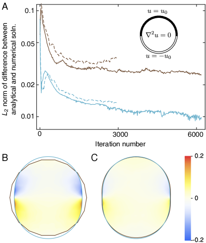
Figure 3: Convergence to the conformal mapping solution for a flexible capacitor with $\Gamma_{\sigma}=2$ and $\Gamma_{W}=1$. A Norm of the difference between simulation and conformal mapping results for the field (brown) and shape (cyan) for simulations with (solid) and without (dashed) the regularization routine as the simulation reaches convergence. Comparison plots of the B initial and C final states of the simulation. The outer borders of the CM (cyan) and simulation (brown) solutions are shown, and points interior to both shapes are shaded by the difference between the field solutions at those points.

To remedy this, two auxiliary functionals are introduced to regularize the problem. The first,

$$E_{R,energy}=\sum_{i}^{N_{f}}\left[\int_{D_{i}}(\nabla u)^{2}dA-\frac{\int_{D}(\nabla u)^{2}dA}{N_{f}}\right]^{2},$$ (9)

prefers to maintain equal energy density among all triangles; the second,

$$E_{R,angle}=\sum_{i}^{N_{f}}\left[\frac{1}{\pi}\sum_{j=1}^{3}(\psi_{i,j}-\pi/3)^{2}\right],$$ (10)

favors triangles with equal angles. In (9) and (10), $\psi_{i,j}$ is the interior angle of face $i$ at vertex $j$ and $N_{f}$ is the total number of triangles composing the mesh. Using the algorithm described in the previous section, gradient descent is performed by successive line searches on the target and auxiliary functionals.

To validate our algorithm, we take advantage the fact that an approximate analytical solution is available from conformal mapping, at least in the limit of small deformations. We use a one-parameter area conserving conformal map $z(w)$ of the form,

$$z=w\sqrt{1-3\alpha^{2}}+\alpha w^{3}.$$ (11)

to map the undeformed capacitor, i.e. the unit disk, parametrized by complex coordinates $w$, to a target domain with coordinates $z$. The electric potential is also represented in the source domain with a complex function $u(w)$,

$$u(w)=\Im\left(\sum_{n=1}^{\infty}c_{n}w^{n}\right),$$ (12)

with coefficients $c_{n}$. By translating the energy functional (8) into complex form, inserting the map eq. (11) and potential eq. (12), and performing the integrations, we obtain an expression for the energy that is quadratic in $\alpha$ and $c_{n}$ and readily minimized numerically. Full details of the derivation are provided in the appendix.

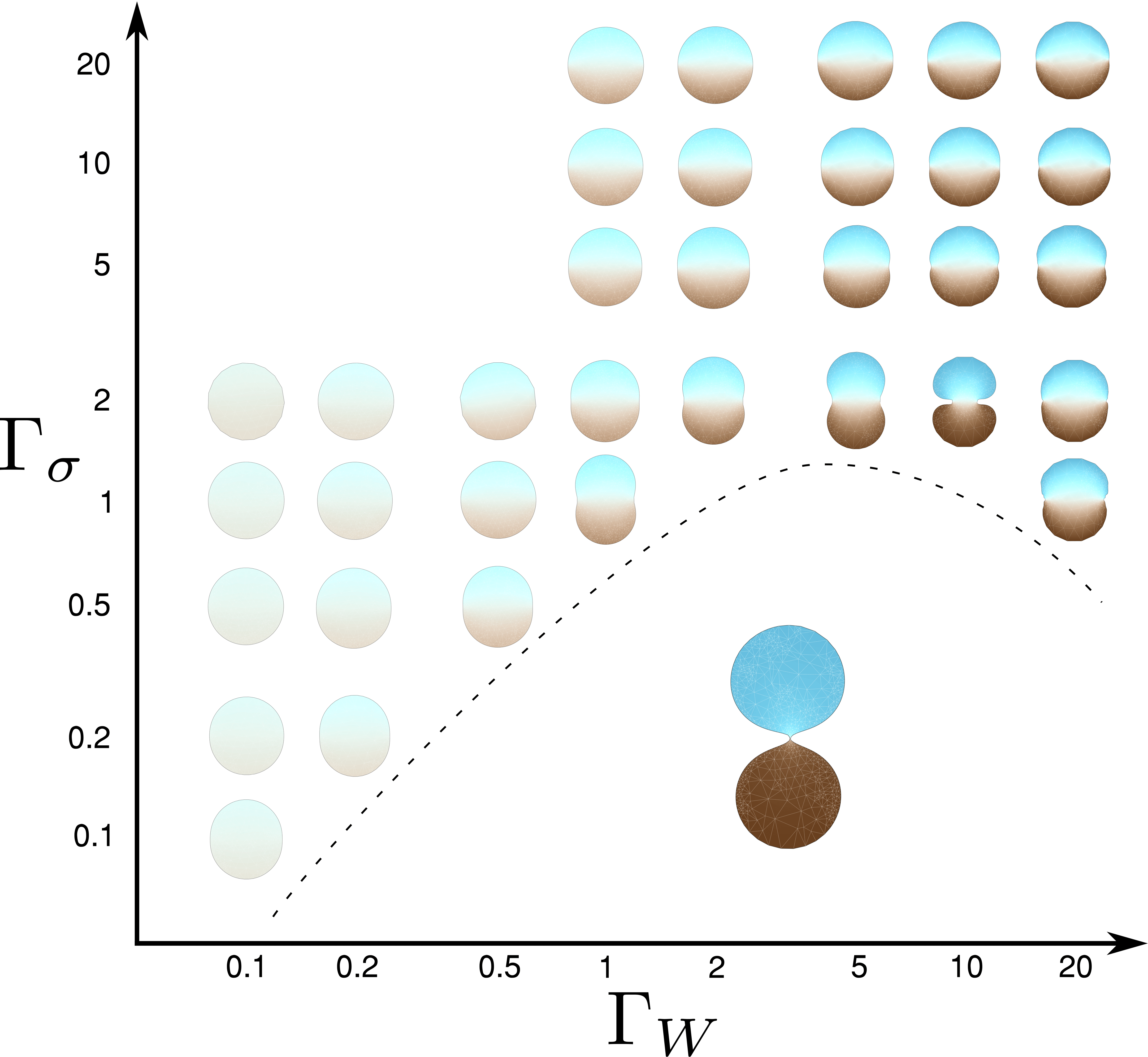
Figure 4: Shape of a flexible capacitor with applied electric field. Deep cyan (brown) regions indicate a field value of $+u_{0}$ ($-u_{0}$). All cases were started with a circular shape and a field that changes linearly along the vertical. Solutions below the dashed line converge on a “pinched” configuration that prefers to separate.

For a test case with parameters $\Gamma_{\sigma}=2$ and $\Gamma_{W}=1$, we show in fig. 3A a comparison between the conformal mapping solution and the finite element solution as a function of iteration for the $L_{2}$ norm of the difference in the field,

$$\left\|u_{c}-u_{fe}\right\|_{2}=\int|u_{c}-u_{fe}|^{2}dA,$$

and the $L_{2}$ norm of the difference in shape, i.e. the area between the finite element boundary and the conformal mapping boundary. Both quantities converge to a fixed nonzero value because the conformal mapping solution is itself approximate. Additionally, we show these quantities with and without the regularization scheme active. Note that without regularization, the method fails to converge due to bunching of the mesh points. In figure fig. 3B and fig. 3C, a local comparison between the conformal mapping and finite element solution is shown for the start and end configurations, showing a good agreement.

In figure 4 we display configurations that result from these minimizations as a function of $\Gamma_{W}$ and $\Gamma_{\sigma}$ including those that exhibit large deformations outside the validity of the conformal mapping solution. For $\sigma>W$, the capacitors tend to remain fairly circular; as $\Gamma_{W}$ is increased the solution conforms more closely to the boundary conditions. Conversely, for $\sigma<W$ significant deformations of the capacitor are allowed; the shape elongates vertically at the expense of horizontal invaginations. Beneath the dashed line in fig. 4, the deformation is so extreme that the invaginations meet; if allowed to, the capacitor would seperate into two disconnected domains.

III.2 Tactoids

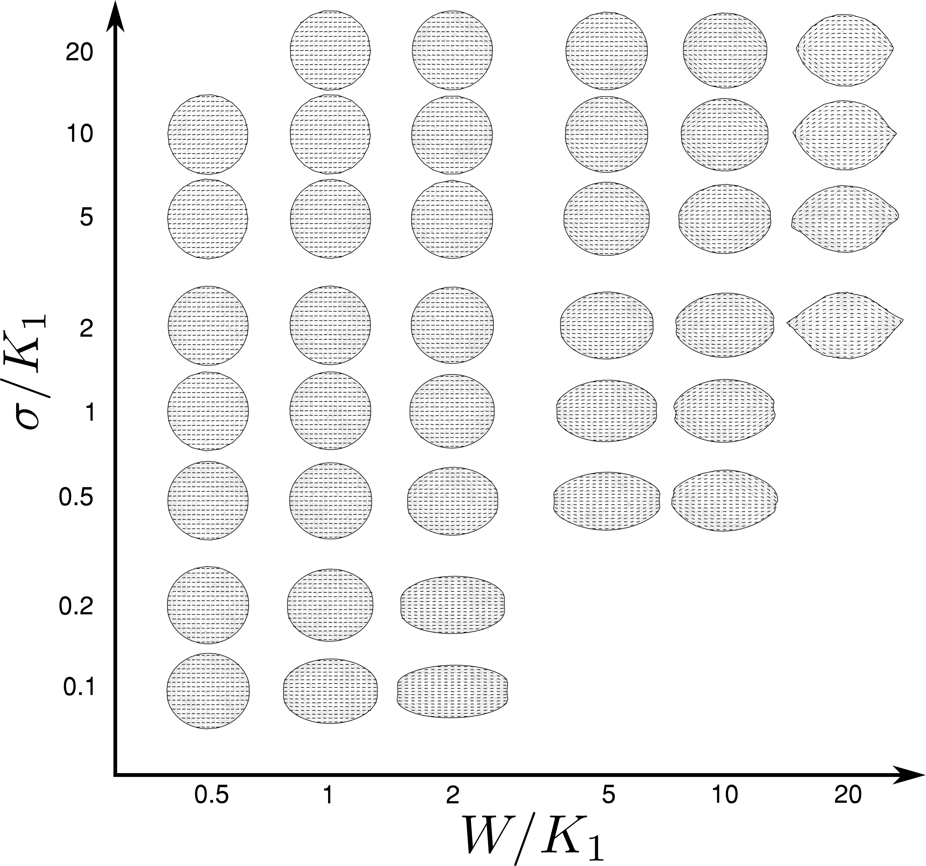
Figure 5: Shape of a nematic droplet. All cases were started with a circular shape and a director field with virtualized defects on the horizontal axis. Depending on the anchoring strength, these defects may spread out to infinity or may move into the droplet.

We now adapt the simulation developed in the previous section to study nematic tactoids. Parametrizing the director as $\mathbf{n}=(\sin\theta,\cos\theta)$, the energy functional contains line tension, elastic and anchoring terms respectively,

$$E = \sigma\int_{\partial D}dl+\Lambda\int_{D}\left[K_{1}\left(\nabla\cdot\mathbf{n}\right)^{2}+K_{3}\left|\nabla\times\mathbf{n}\right|^{2}\right]dA$$

$$+W\int_{\partial D}(\theta-\theta_{e})^{2}dl$$

where $K_{1}$ and $K_{3}$ are the splay and bend elastic constants respectively. This is to be minimized subject to an area constraint as before, and we divide through by $\Lambda K_{1}$ and make the change of variables $x\rightarrow\Lambda x^{\prime}$ in order to non-dimensionalize the energy.

When $K_{3}=K_{1}$, the elastic energy density reduces to $K_{1}\left(\nabla\theta\right)^{2}$ and the problem is almost exactly the same as that discussed in the previous section, with one important difference: the easy axis $\theta_{e}$ is not fixed on the boundary, but dynamically determined at each iteration relative to the local estimate of the tangent plane. Even so, we use the same regularization functionals and algorithm, only inserting a modified force functional for the elastic anisotropy.

In figure 5, a set of equilibrium shapes is shown for $K_{3}=K_{1}$ as a function of $\sigma/K_{1}$ and $W/K_{1}$. In all cases, the minimization was started from a circular initial configuration, with virtual defects outside the tactoid. Stronger anchoring causes the nematic to better conform to the boundary condition, effectively moving the virtual defects closer to the surface of the droplet. Weaker line tension, on the other hand, permits more elongation of the droplet.

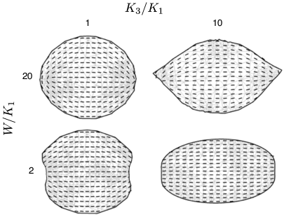
Figure 6: Simulations of nematic droplets with weak line tension ($W/\sigma=10$). Line segments indicate the director orientation at those points.

The effect of elastic anisotropy is shown in fig. 6, which displays four equilibrium configurations as a function of $K_{3}/K_{1}$ and $W/K_{1}$. It is clear that significant shape deformation is only achieved with the introduction of elastic anisotropy. Stronger elastic constants lead to a fairly homogeneous field with excluded defects, while weak elastic constants allow the field the better follow the anchoring condition, resulting in a pair of boojum defects.

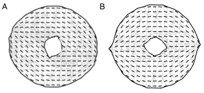
Figure 7: Simulations of nematic droplets with weak line tension ($W/\sigma=10$) with interior holes. The holes in the droplets form negative tactoids that align either A perpendicular or B parallel to the orientation of the outer tactoid depending on the ratio of $W$ to $K_{1}$.

It is straightforward to apply our technique to more complicated geometries, such as non-simply connected domains. In figure 7, we display two equilibrium configurations with negative tactoid holes on the interior. These were started from an initially annular configuration with an area constraint additionally applied to the hole. Solutions with the interior negative tactoid aligned perpendicular to (fig. 7A) or parallel to (fig. 7B) with the exterior were found.

We note that the array of achievable tactoid shapes fit within the classes defined in Prinsen and van der Schoot (2003). Additionally, the shape trends displayed in fig. 5 closely mimic those proposed by Lishchuk Lishchuk and Care (2004). Unique to our results is the ability to predict tactoid shapes with more complex boundaries. This allows for better agreement with experimentally produced cusped ellipsoids Tortora and Lavrentovich (2011); Kaznacheev et al. (2002), as well as tactoids containing isotropic inclusions Casagrande et al. (1987); Kim et al. (2013). Excitingly, experimental evidence of the latter tends to produce negative tactoids that align parallel to the exterior tactoid, in agreement with one of our classes.

IV Conclusion

The present work describes our initial exploration of a very challenging class of problems, where the equilibrium configuration of a system must be found by minimizing some functional with respect to internal fields as well as the shape of the domain. Gradient descent methods are effective for some subset of these problems, and form the basis of programs like Surface Evolver, but require management of mesh quality during the minimization. Some of the challenges were illustrated with a toy example of minimizing the length of a loop at constant area, showing that mesh points become bunched during the minimization and prevent convergence on the correct solution.

A regularization strategy was shown to be effective in overcoming these difficulties whereby the target functional was supplemented with an auxiliary functional to promote equally-spaced mesh points. The same approach was used to develop a solver for the equilibrium configuration of a flexible capacitor, as well as that of a 2D nematic tactoid. Exploring the space of shapes as a function of the surface tension and anisotropic elastic constants, we found structures similar to those experimentally observed, as well as some others predicted in the literature. We are presently working to generalize our program to work with higher dimensional manifolds, arbitary combinations of fields defined upon them, a broader selection of energy functionals and dynamics problems.

Appendix: Conformal Mapping Solution

The integrals in (6) and (7) must be translated into complex notation using the map $z(w)$. To do this, we use familiar properties of complex functions, i.e that $\frac{dz}{dw}$ plays the role of a metric, so that lengths transform under the action of $z$ like $\left|\frac{dz}{dw}\right|$ and areas transform like $\left|\frac{dz}{dw}\right|^{2}$. Parametrizing the boundary of the unit circle as $e^{i\theta}$, the program in complex notation is to minimize,

$$E=\Gamma_{\sigma}\int\left|\frac{dz}{dw}\right|d\theta+\Gamma_{\epsilon}\int\left|\frac{du}{dw}\right|^{2}dw+\int(u-u_{0})\left|\frac{dz}{dw}\right|d\theta,$$ (13)

with respect to $z(w)$ and the real function $u(w)$ and subject to the constraint,

$$\frac{1}{2}\int\bar{z}\frac{dz}{dw}ie^{i\theta}d\theta=\pi,$$ (14)

where we used the property that the electrostatic energy is invariant under a conformal mapping.

The conformal map $z(w)$ and the scalar potential $u$ are expanded as a power series in $w$,

$$z(w)=\sum_{n=1}^{\infty}a_{n}w^{n},$$ (15)

and

$$u(w)=\Im\left(\sum_{n=1}^{\infty}c_{n}w^{n}\right),$$ (16)

where positive powers only have been retained to ensure regularity at the origin $w=0$ and the imaginary part is chosen due to the symmetry of the boundary condition. Substituting $w=re^{i\theta}$ into (16), we obtain

$$u(w)=\sum_{n}c_{n}r^{n}\sin(n\theta),$$ (17)

and turn to the issue of evaluating each term in the energy functional, as well as the area constraint, in order of difficulty.

The first term we consider is the electrostatic energy, which is after all invariant under the mapping. Inserting the solution (17) into the second term in (13) yields,

$$E_{el}=\Gamma_{\epsilon}\sum_{n}\frac{2n^{2}}{2n-1}c_{n}^{2}.$$ (18)

Next, we turn to the area constraint. Inserting (15) into (14) and integrating,

$$A=\sum_{n}n\pi a_{n}^{2}.$$

At this point, we shall specialize the problem to only consider the first two odd terms of $z(w)$,

$$z=a_{1}w+a_{3}w^{3}$$ (19)

where the first is the identity mapping and the second represents the first nonzero term of the deformation induced by the field. This approximation is equivalent to assuming that the capacitor is only weakly deformed from the circular reference shape, which is true if the line tension dominates in the energy functional. We therefore create a one parameter family of maps that preserves the area of the unit disk,

$$z=w\sqrt{1-3\alpha^{2}}+\alpha w^{3}.$$ (20)

The line tension term in (13) is highly nonlinear. Inserting the restricted map (20) and evaluating using $w=e^{i\theta}$ on the boundary, we obtain

$$E_{lt}=\Gamma_{\sigma}\int_{-\pi}^{\pi}\sqrt{9\alpha^{2}\sin^{2}(2\theta)+\left(\sqrt{1-3\alpha^{2}}+3\alpha\cos(2\theta)\right)^{2}}d\theta,$$

which may be evaluated in terms of the complete elliptic integral $\text{E}(m)$,

$$F_{lt}=2\Gamma_{\sigma}\left[G_{+}E\left(m_{+}\right)+G_{-}E\left(m_{-}\right)\right],$$

where

$$G_{\pm} = \sqrt{1+6\alpha\left(\alpha\pm\sqrt{1-3\alpha^{2}}\right)},$$

$$m_{\pm} = \frac{\pm 12\alpha\sqrt{1-3\alpha^{2}}}{1+6\alpha\left(\alpha\pm\sqrt{1-3\alpha^{2}}\right)}.$$

Due to the complexity of this expression, we make a series expansion about $\alpha=0$ and retain the first nontrivial term,

$$E_{lt}\approx\Gamma_{\sigma}\pi\left(2+\frac{3}{2}\alpha^{2}\right).$$ (21)

The anchoring term also contains $\left|\frac{dz}{dw}\right|$, and hence is also nonlinear. We follow a similar strategy to the line tension, expanding this in powers of $\alpha$ on the boundary $w=e^{i\theta}$ and retaining only terms up to quadratic order,

$$\left|\frac{dz}{dw}\right|\approx 1+3\alpha\cos(2\theta)-\frac{3}{4}\alpha^{2}(3\cos(4\theta)-1).$$

Inserting this, together with the series solution for $u$, eq. (17), into the anchoring energy term in (13) and performing the integration yields an expression of the form,

$$E_{a}=\left(p+q_{i}c_{i}+r_{ij}c_{i}c_{j}\right),$$ (22)

where $p$, $q$ and $r$ are scalar, vector and matrix quadratic functions of $\alpha$. $r_{ij}$ is a symmetric band-diagonal matrix with a checkerboard structure, $r_{ij}=0$ if $\left|i-j\right|=0$. For the sake of brevity, we do not list these elements here; they are available in a Mathematica notebook provided as supplementary material.

All terms in the free energy (13) have now been evaluated in terms of the parameter $\alpha$ that defines the area-preserving conformal map (20) as well as the coefficients of the field (17). Expressions for line tension, electric energy and anchoring are quoted in equations (21), (18) and (22) respectively. It may therefore be seen that the total free energy can be put into the form,

$$E=P+Q_{i}c_{i}+R_{ij}c_{i}c_{j},$$ (23)

where $P$, $Q$ and $R$ are quadratic functions of $\alpha$. The scalar $P$ contains contributions from the anchoring and line tension terms; $Q$ contains only contributions from the anchoring term; $R$ contains electrostatic (on the diagonal) and anchoring contributions. The special structure arises because the series expansion in $z$ is low order, while the expansion in $u$ was carried out to arbitrary order and is valid for the situation where the shape deformation is small. A higher order expansion in $z$ will yield $P$, $Q$ and $R$ that are also variables of higher order parameters $\{\beta,\gamma,...\}$. Furthermore, series expansion of $\left|\frac{dz}{dw}\right|$ limits the order of $P$, $Q$ and $R$ to being quadratic in $\alpha$; this expansion could easily be extended further.

Minimization of eq. (23) with respect to $\alpha$ and $c_{i}$ yields the following system of equations,

$$\frac{\partial E}{\partial\alpha}=\frac{\partial P}{\partial\alpha}+\frac{\partial Q_{i}}{\partial\alpha}c_{i}+\frac{R_{ij}}{\partial\alpha}c_{i}c_{j} = 0,$$

$$2R_{ij}c_{j}+Q_{i} = 0,$$ (24)

where we note that $i$ is a free index in the second equation. These equations are efficiently solved by the nested iteration scheme,

$$a^{m+1} = \alpha^{m}-\lambda\left.\frac{\partial F}{\partial\alpha}\right|c_{i}^{m}$$

$$2R_{ij}(\alpha^{m})c_{j}^{m+1} = -Q_{i}(\alpha^{m})$$

for sufficiently small stepsize $\lambda$ and a single initial seed value $\alpha^{0}=0$. A Mathematica notebook that implements this scheme is presented as supplementary material.

References

- Barbero and Evangelista (2005) G. Barbero and L. Evangelista, Adsorption Phenomena and Anchoring Energy in Nematic Liquid Crystals, Liquid Crystals Book Series (CRC Press, 2005), ISBN 9781420037456.
- Rasing and Musevic (2013) T. Rasing and I. Musevic, Surfaces and Interfaces of Liquid Crystals (Springer Berlin Heidelberg, 2013), ISBN 9783662101575.
- Kim et al. (2002) J.-H. Kim, M. Yoneya, and H. Yokoyama, Nature 420, 159 (2002).
- Atherton and Adler (2012) T. J. Atherton and J. H. Adler, Phys. Rev. E 86, 040701 (2012).
- Kondrat et al. (2005) S. Kondrat, a. Poniewierski, and L. Harnau, Liq. Cryst. 32, 95 (2005).
- Anquetil-Deck et al. (2013) C. Anquetil-Deck, D. J. Cleaver, J. P. Bramble, and T. J. Atherton, Phys. Rev. E 88, 012501 (2013).
- Lagerwall and Scalia (2012) J. P. Lagerwall and G. Scalia, Current Applied Physics 12, 1387 (2012).
- MacKintosh and Lubensky (1991) F. C. MacKintosh and T. C. Lubensky, Phys. Rev. Lett. 67, 1169 (1991).
- Fernández-Nieves et al. (2007) A. Fernández-Nieves, V. Vitelli, A. S. Utada, D. R. Link, M. Márquez, D. R. Nelson, and D. A. Weitz, Physical review letters 99, 157801 (2007).
- Whitmer et al. (2013) J. K. Whitmer, X. Wang, F. Mondiot, D. S. Miller, N. L. Abbott, and J. J. de Pablo, Phys. Rev. Lett. 111, 227801 (2013).
- Zocher (1925) V. H. Zocher, Zeitschrift für Anorg. und Allg. Chemie 147, 91 (1925), ISSN 1521-3749.
- Zocher and Jacobsohn (1929) V. H. Zocher and K. Jacobsohn, Kolloid Beih. 28, 167 (1929).
- Bernal and Fankuchen (1941) J. D. Bernal and I. Fankuchen, J. Gen. Physiol. 25, 111 (1941), ISSN 0022-1295.
- Sonin (1998) A. S. Sonin, J. Mater. Chem. 8, 2557 (1998), ISSN 09599428.
- Tang et al. (2005) J. X. Tang, H. Kang, and J. Jia, Langmuir 21, 2789 (2005), ISSN 07437463.
- Casagrande et al. (1987) C. Casagrande, P. Fabre, M. A. Guedeau, and M. Veyssie, Europhys. Lett. 3, 73 (1987), ISSN 0295-5075.
- Kim et al. (2013) Y.-K. Kim, S. V. Shiyanovskii, and O. D. Lavrentovich, J. Phys. Condens. Matter 25, 404202 (2013), ISSN 1361-648X, eprint 1303.6239.
- Verhoeff et al. (2011) A. A. Verhoeff, I. A. Bakelaar, R. H. J. Otten, P. Van Der Schoot, and H. N. W. Lekkerkerker, Langmuir 27, 116 (2011), ISSN 07437463.
- Peng and Lavrentovich (2015) C. Peng and O. D. Lavrentovich, Soft Matter 11, 10 (2015), ISSN 1744-683X, eprint 1507.07499.
- Mushenheim et al. (2014) P. C. Mushenheim, R. R. Trivedi, D. B. Weibel, and N. L. Abbott, Biophys. J. 107, 255 (2014), ISSN 15420086.
- Zhou et al. (2014) S. Zhou, A. Sokolov, O. D. Lavrentovich, and I. S. Aranson, Proc. Natl. Acad. Sci. U. S. A. 111, 1265 (2014), ISSN 1091-6490, eprint 1312.5359.
- Dogic and Fraden (2001) Z. Dogic and S. Fraden, Philos. Trans. R. Soc. A Math. Phys. Eng. Sci. 359, 997 (2001), ISSN 1364-503X.
- Chandrasekhar (1966) S. Chandrasekhar, Mol. Cryst. Liq. Cryst. 2, 71 (1966), ISSN 0369-1152.
- Kaznacheev et al. (2003) A. V. Kaznacheev, M. M. Bogdanov, and A. S. Sonin, J. Exp. Theor. Phys. 97, 1159 (2003), ISSN 1063-7761.
- Kaznacheev et al. (2002) A. V. Kaznacheev, M. M. Bogdanov, and S. A. Taraskin, J. Exp. Theor. Phys. 95, 57 (2002).
- Prinsen and van der Schoot (2003) P. Prinsen and P. van der Schoot, Phys. Rev. E. Stat. Nonlin. Soft Matter Phys. 68, 021701 (2003), ISSN 1063-651X.
- Prinsen and Van Der Schoot (2004) P. Prinsen and P. Van Der Schoot, Eur. Phys. J. E 13, 35 (2004), ISSN 12928941.
- Bates (2003) M. A. Bates, Chem. Phys. Lett. 368, 87 (2003), ISSN 00092614.
- Vanzo et al. (2012) D. Vanzo, M. Ricci, R. Berardi, and C. Zannoni, Soft Matter 8, 11790 (2012), ISSN 1744-683X.
- Warner and Terentjev (2003a) M. Warner and E. Terentjev, Liquid Crystal Elastomers (Oxford Science Publications, 2003a).
- De Gennes (1975) P. G. De Gennes, C. R. Acad. Sci. B 281, 101 (1975).
- Kundler and Finkelmann (1995) I. Kundler and H. Finkelmann, Macromol. Rapid Commun. 16, 679 (1995).
- Finkelmann et al. (2001) H. Finkelmann, E. Nishikawa, G. Pereira, and M. Warner, Physical Review Letters 87, 015501 (2001), ISSN 0031-9007.
- Conti et al. (2002) S. Conti, A. DeSimone, and G. Dolzmann, Physical Review E 66, 061710 (2002), ISSN 1063-651X.
- Mbanga et al. (2010a) B. L. Mbanga, F. Ye, J. V. Selinger, and R. L. B. Selinger, Phys. Rev. E 82, 051701 (2010a).
- Chang et al. (1997) C.-C. Chang, L.-C. Chien, and R. Meyer, Physical Review E 56, 595 (1997), ISSN 1063-651X.
- Burridge et al. (2006) D. Burridge, Y. Mao, and M. Warner, Physical Review E 74, 021708 (2006), ISSN 1539-3755.
- Menzel and Brand (2007) A. Menzel and H. Brand, Physical Review E 75, 011707 (2007), ISSN 1539-3755.
- Ye et al. (2007) F. Ye, R. Mukhopadhyay, O. Stenull, and T. Lubensky, Physical Review Letters 98, 147801 (2007), ISSN 0031-9007.
- Urayama et al. (2003) K. Urayama, Y. Okuno, and S. Kohjiya, Macromolecules 36, 6229 (2003), ISSN 0024-9297.
- Urayama et al. (2006) K. Urayama, R. Mashita, Y. O. Arai, and T. Takigawa, Macromolecules 39, 8511 (2006), ISSN 0024-9297.
- Yu et al. (2003) Y. Yu, M. Nakano, and T. Ikeda, Nature 425, 145 (2003), ISSN 1476-4687.
- Li et al. (2003) M.-H. Li, P. Keller, B. Li, X. Wang, and M. Brunet, Advanced Materials 15, 569 (2003), ISSN 1521-4095.
- Camacho-Lopez et al. (2004) M. Camacho-Lopez, H. Finkelmann, P. Palffy-Muhoray, and M. J. Shelley, Nature materials 3, 307 (2004), ISSN 1476-1122.
- He (2007) L. He, Physical Review E 75, 041702 (2007), ISSN 1539-3755.
- Sawa et al. (2010) Y. Sawa, K. Urayama, T. Takigawa, A. DeSimone, and L. Teresi, Macromolecules 43, 4362 (2010), ISSN 0024-9297.
- Mahimwalla et al. (2012) Z. Mahimwalla, K. Yager, J.-i. Mamiya, A. Shishido, A. Priimagi, and C. Barrett, Polymer Bulletin 69, 967 (2012), ISSN 0170-0839.
- Yu et al. (2002) Y. Yu, M. Nakano, and T. Ikeda, Nature 425, 145 (2002).
- Warner and Terentjev (2003b) M. Warner and E. Terentjev, Macromolecular Symposia 200, 81 (2003b), ISSN 1521-3900.
- Palfffy-Muhoray (2009) P. Palfffy-Muhoray, Nat. Mater. 8, 614 (2009).
- Xie and Zhang (2005) P. Xie and R. Zhang, J. Mater. Chem. 15, 2529 (2005).
- Mbanga et al. (2010b) B. L. Mbanga, F. Ye, J. V. Selinger, and R. L. Selinger, Physical Review E 82, 051701 (2010b).
- de Haan et al. (2014) L. T. de Haan, V. Gimenez-Pinto, A. Konya, T.-S. Nguyen, J. M. N. Verjans, C. Sánchez-Somolinos, J. V. Selinger, R. L. B. Selinger, D. J. Broer, and A. P. H. J. Schenning, Advanced Functional Materials 24, 1251 (2014), ISSN 1616-3028.
- Brakke (1992) K. A. Brakke, Experimental mathematics 1, 141 (1992).
- Lishchuk and Care (2004) S. V. Lishchuk and C. M. Care, Phys. Rev. E - Stat. Nonlinear, Soft Matter Phys. 70, 1 (2004), ISSN 15393755.
- Tortora and Lavrentovich (2011) L. Tortora and O. D. Lavrentovich, Proc. Natl. Acad. Sci. U. S. A. 108, 5163 (2011), ISSN 0027-8424.