Two loop correction to interference in $gg\to ZZ$

Abstract

We present results for the production of a pair of on-shell $Z$ bosons via gluon fusion. This process occurs both through the production and decay of the Higgs boson, and through continuum production where the $Z$ boson couples to a loop of massless quarks or to a massive quark. We calculate the interference of the two processes and its contribution to the cross section up to and including order $O(\alpha_{s}^{3})$. The two-loop contributions to the amplitude are all known analytically, except for the continuum production through loops of top quarks of mass $m$. The latter contribution is important for the invariant mass of the two $Z$ bosons, (as measured by the mass of their leptonic decay products, $m_{4l}$), in a regime where $m_{4l}\geq 2m$ because of the contributions of longitudinal bosons. We examine all the contributions to the virtual amplitude involving top quarks, as expansions about the heavy top quark limit combined with a conformal mapping and Padé approximants. Comparison with the analytic results, where known, allows us to assess the validity of the heavy quark expansion, and it extensions. We give results for the NLO corrections to this interference, including both real and virtual radiation.

1 Introduction

The production of four charged leptons is a process of great importance at the LHC. It was one of the discovery channels of the Higgs boson at the LHC. It also provides fundamental tests of the gauge structure of the electroweak theory through the high energy behaviour. Four charged leptons are predominantly produced by quark anti-quark annihilation; the mediation is by photons or $Z$ bosons dependent on the mass of the four leptons, $m_{4l}$.

A smaller contribution, which however grows with energy is provided by gluon-gluon fusion. The Higgs boson is of course produced in this channel; in the Standard Model (SM) this occurs predominantly through the mediation of a loop of top quarks. As pointed out by Kauer and Passarino Kauer:2012hd , despite the narrow width of the Higgs boson, the Higgs-mediated diagram gives a significant contribution for $m_{4l}>m_{H}$. If we examine the tail of the Higgs-mediated diagrams there are three phenomena occurring:

• The opening of the threshold for the production of real on-shell $Z$ bosons, $m_{4l}>2m_{Z}$.

• The region $m_{4l}=2m$, ($m$ is the top quark mass) where the loop diagrams develop an imaginary part.

• The large $m_{4l}$ region, $m_{4l}>2m$, where the destructive interference between the Higgs-mediated diagrams leading to $Z$ bosons and the continuum production of on-shell $Z$ bosons is most important.

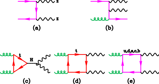
Figure 1: Representative diagrams for the $ZZ$ production. In the following we will suppress the $Z$-decays to leptons.

A feature of this tail is that it depends on the couplings of the Higgs boson to the initial and final state particles but not on the width of the Higgs boson. Assuming the couplings of the on- and off-peak Higgs-mediated amplitudes are the same, it has been proposed to use this property to derive upper bounds on the width of the Higgs boson Caola:2013yja . Note that models with different on- and off-peak couplings can be constructed Englert:2014aca .

In the following we shall refer to the production of the bosons $V_{1},V_{2}$. Gluon-gluon fusion first contributes to the cross section for electroweak gauge boson production $pp\to V_{1}V_{2}$ as shown in Fig. 1(c)-(e) at ${\cal O}(\alpha_{S}^{2})$, which is the next-to-next-to-leading-order (NNLO) with respect to the leading-order (LO) QCD process shown in Fig. 1(a); no two-loop $gg\to V_{1}V_{2}$ amplitudes participate in this order in perturbation theory.

In the context of the Higgs boson width, however, the interference between the Higgs-mediated $Z$ boson pair-production and the Standard Model continuum at next-to-leading-order (NLO) QCD already requires knowledge of the one- and two-loop $gg\to(H\to)V_{1}V_{2}$ amplitudes. The requirement for more precise estimates to the Higgs boson width were emphasised in ATLAS-CONF-2014-042 ; Khachatryan:2014iha ; Melnikov:2015laa . Signal-background interference effects beyond the leading order have been considered in ref. Bonvini:2013jha for the process $gg\to H\to W^{+}W^{-}$ for the case of a heavy Higgs boson.

In this work we will limit ourselves to the $Z$ boson pair final state, due to its importance at the LHC. At LO Dawson:1993qf and NLO Spira:1995rr ; Harlander:2005rq ; Anastasiou:2006hc ; Aglietti:2006tp the amplitudes for single Higgs boson production have been known for quite some time. At LO, the amplitude for the SM continuum $gg\to ZZ$ process occurs via massless and massive fermion loops and results are available in each case  Glover:1988rg ; Kauer:2012ma ; Campbell:2013una ; Campbell:2014gua .

The situation, however, is different for the NLO continuum process, although vast progress in terms of two-loop amplitudes has been made Gehrmann:2014bfa ; Cascioli:2014yka ; Caola:2014iua ; Gehrmann:2015ora ; Caola:2015ila ; vonManteuffel:2015msa . Recently two-loop $gg\to ZZ$ amplitudes via massless quarks became available Caola:2015ila ; vonManteuffel:2015msa . The complete computation of two-loop amplitudes with massive internal quark loops, on the other hand, is commonly assumed to be just beyond present technical capabilities. Although the contribution of the top quark loops to these diagrams is smaller than the contribution of the light quarks in the region just above the $Z$-pair threshold, in the high $m_{4l}$ region the amplitude is dominated by the contributions of longitudinal $Z$ bosons that couple to the top quark loops. Recently a first heavy top quark approximation for the two-loop $gg\to ZZ$ amplitude with internal top quarks was published Melnikov:2015laa . In that work only the leading term in the $s/m^{2}$ expansion was considered. In that approximation, the vector-coupling of the $Z$ boson to the top quark does not contribute. In addition an approximate treatment of this process at higher orders, based on soft gluon resummation, was presented in Ref. Li:2015jva .

In the present work we will push this analysis further. We start by presenting our results for the LO and NLO Higgs-mediated $ZZ$ production in terms of the $s/m^{2}$ expansion in Sec. 2, despite the fact that the full result is known. This part is required for the later interference with the SM continuum. Furthermore, it is well suited to introduce our notation in Sec. 2.1 and to assess the validity of the approximation methods with respect to the exact known (N)LO amplitudes in Sec. 2.2.

The results for the LO and virtual NLO contributions to the SM continuum with massive quark loops will be given in Sec. 3 as a large-mass expansion (LME) with terms up to $(s/m^{2})^{6}$. We will limit our discussion to the interference between the Higgs-mediated term and the continuum term. Similar to Melnikov:2015laa we will consider on-shell $Z$ bosons in the final state. A theoretical predictions for off-shell $Z$ bosons would be optimal, but in order to reduce the number of scales in the problem, we restrict ourselves to on-shell $Z$ bosons. Since we are primarily interested in the high-mass behaviour this is an appropriate approximation. A limited number of scales is beneficial when we consider the extension of our approach to a full calculation. In Sec. 4 we summarize our treatment of the real radiation contribution, which makes use of results already presented in Ref. Campbell:2014gua .

The results of our calculation, including loops of both massless and massive quarks, will be presented in Sec. 5. We will compare the effects of the NLO corrections to the interference contribution with the corresponding corrections to the Higgs diagrams alone. In addition, we will discuss the impact of our results on analyses of the off-shell region that aim to bound the Higgs boson width.

All expansion results from Sec. 2 and Sec. 3.4.1 are provided via ancillary files on arXiv as FORM and Mathematica readable code.

2 Higgs Production in Gluon Fusion and Decay to $ZZ$

In this section we give a detailed discussion of single Higgs boson production at LO and NLO QCD and its subsequent decay to a pair of on-shell $Z$ bosons. As mentioned earlier the LO and NLO amplitudes for single Higgs boson production have been known for a long time; either approximate results in terms of Taylor expansions in the inverse of the top quark mass $s/m^{2}$ Dawson:1990zj ; Dawson:1993qf ; Harlander:2002wh ; Anastasiou:2002yz ; Aglietti:2006tp ; Harlander:2009bw ; Pak:2009bx or results keeping the exact top mass dependence Djouadi:1991tka ; Aglietti:2006tp .

It is understood that, whenever feasible and available, the exact results for LO and NLO amplitudes are used. However, we are mainly interested in approximations to the interference contributions ${\rm Re}\bra{{\cal A}_{\text{LO}}}\ket{{\cal B}_{\text{(N)LO}}}$, where ${\cal A}$ denotes the Higgs-mediated and ${\cal B}$ the SM continuum amplitude. Since no exact results are available for ${\cal B}_{\text{NLO}}$ we will use the, so-called, large-mass expansion Smirnov:2002pj as an approximation of the SM continuum. Hence, for consistency, we also perform the expansion of the Higgs-mediated amplitude ${\cal A}$ to high powers in $s/m^{2}$. Expansion of the two-loop Higgs-mediated amplitude ${\cal A}_{\text{NLO}}$ and its comparison to available results from the literature provides moreover a helpful check of our expansion routines due to the general structure of the LME.

Furthermore, the large-mass expansion in powers of $s/m^{2}$ is formally only valid below the threshold of top quark pair-production, as $m$ is assumed to be much larger than any other scale in the problem, e.g. $s\ll m^{2}$. As extensively discussed in literature the naive LME can be drastically improved at (and even far above) threshold by taking the next mass threshold into account, see Ref Smirnov:2002pj and references within, or by rescaling the approximated NLO result by the exact LO result, see e.g. Refs Pak:2009dg ; Grigo:2013rya . We will address this issue in Sec. 2.2.3 and try to draw conclusions for the SM continuum.

2.1 Preliminaries

The amplitudes for single Higgs boson production

$$g(p_{1},\alpha,A)+g(p_{2},\beta,B)\to H(p_{1}+p_{2}),\;\;s=(p_{1}+p_{2})^{2}\,,$$ (1)

are illustrated in Fig. 2 for the one-loop and two-loop case.

(a)

(b)

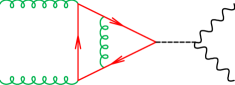
(c)

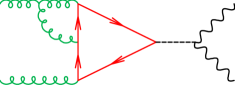
(d)

Figure 2: Representative diagrams for the LO+NLO virtual $gg\to H\to ZZ$ amplitude.

The largest contribution is due to the internal massive top quark loop; in the following we will ignore the contribution of other quarks for the Higgs production process.

The $gg\to H$ amplitude, with color (Lorentz) indices $A,B(\alpha,\beta)$ for the initial state gluons, can be written as

$$\ket{{\cal A}^{0,AB}_{\alpha\beta}(\alpha_{S}^{0},m^{0},\mu,\epsilon)}=-i\delta^{AB}\,\frac{g_{W}}{2m_{W}}\frac{4}{3}\;\left(g_{\alpha\beta}\,p_{1}\cdot p_{2}-p_{1,\beta}p_{2,\alpha}\right)\;\ket{{\cal A}^{0}(\alpha_{S}^{0},m^{0},\mu,\epsilon)}\,,$$ (2)

such that the reduced matrix element $\ket{{\cal A}^{0}(\alpha_{S}^{0},m^{0},\mu,\epsilon)}$ is dimensionless and can be expressed as a function of $\mu^{2}/s$ and $r_{t}=m^{2}/s$. The bare on-shell amplitudes admit the perturbative expansion

$$\ket{{\cal A}^{0}(\alpha_{S}^{0},m^{0},\mu,\epsilon)}=\frac{\alpha_{S}^{0}}{4\pi}\ket{{\cal A}^{0,(1)}(m^{0},\mu,\epsilon)}+\left(\frac{\alpha_{S}^{0}}{4\pi}\right)^{2}\ket{{\cal A}^{0,(2)}(m^{0},\mu,\epsilon)}+{\cal O}{\left((\alpha_{S}^{0})^{3}\right)}\,,$$ (3)

where we introduced the parameter $\epsilon$ from dimensional regularisation in $d=4-2\epsilon$ space-time dimensions and $\mu$ to keep the amplitudes dimensionless. The calculation is performed in Conventional Dimensional Regularisation (CDR) and the following definition of the $d$-dimensional loop integral measure

$$\int{\frac{d^{4}p}{(2\pi)^{4}}}\longrightarrow\mu^{2\epsilon}\underbrace{\frac{e^{\epsilon\gamma_{E}}}{(4\pi)^{\epsilon}}}_{\equiv S_{\epsilon}}\cdot\int{\frac{d^{d}p}{(2\pi)^{d}}}$$ (4)

is used in accordance with the $\overline{MS}$-scheme, to avoid the proliferation of unnecessary $\gamma_{E}-\log(4\pi)$ terms.

The ultraviolet (UV) renormalised amplitudes are given by

$$\ket{{\cal A}^{r}(\alpha_{S}^{(n_{f})}(\mu),m,\mu,\epsilon)}=Z_{m}Z_{g}\ket{{\cal A}^{0}(\alpha_{S}^{0},m^{0},\mu,\epsilon)}\,,$$ (5)

where $Z_{g}$ denotes the on-shell gluon renormalisation constant. The $Ht\bar{t}$ vertex is renormalised, according to Braaten:1980yq , by $g_{H}^{0}=Z_{m}\,g_{H}$ with $g_{H}$ being the Yukawa coupling for the top quark. The bare top quark mass is related to the renormalised mass, $m$, by $m^{0}=Z_{m}m$. The necessary on-shell renormalisation constants are given by

$$Z_{g} =1-\frac{\alpha_{S}^{(n_{f})}}{4\pi}T_{F}\left(\frac{\mu^{2}}{m^{2}}\right)^{\epsilon}\cdot\frac{4}{3\epsilon}+{\cal O}\left((\alpha_{S}^{(n_{f})})^{2},\epsilon\right)\quad\text{and}$$ (6)

$$Z_{m} =1-\frac{\alpha_{S}^{(n_{f})}}{4\pi}C_{F}\left(\frac{\mu^{2}}{m^{2}}\right)^{\epsilon}\left[\frac{3}{\epsilon}+4\right]+{\cal O}\left((\alpha_{S}^{(n_{f})})^{2},\epsilon\right)\,,$$ (7)

with $T_{F}=1/2$. See appendix A of Baernreuther:2013caa and references therein for more information. The mass renormalisation enters as an overall factor in Eq. (5) because of the renormalisation of the Yukawa coupling, and also implicitly in the relationship between the bare and renormalised mass. We will always present mass-renormalised results in the following.

The strong coupling constant is renormalised in the $\overline{MS}$-scheme according to

$$\alpha_{S}^{0}=Z_{\alpha_{S}}^{(n_{f})}\alpha_{S}^{(n_{f})}(\mu)\,,$$ (8)

with Baernreuther:2013caa

$$Z_{\alpha_{S}}^{(n_{f})}=1-\frac{\alpha_{S}^{(n_{f})}}{4\pi}\frac{\beta_{0}^{(n_{f})}}{\epsilon}+{\cal O}\left((\alpha_{S}^{(n_{f})})^{2}\right)\quad\text{and}\quad\beta_{0}^{(n_{f})}=\frac{11}{3}C_{A}-\frac{4}{3}T_{F}n_{f}\,,$$ (9)

where $n_{f}=6$ denotes the number of fermions and $\beta_{0}^{(n_{f})}$ the coefficient of the beta function. The explicit scale dependence of the renormalised strong coupling constant $\alpha_{S}^{(n_{f})}(\mu)$ is dropped in the following to simplify our notation. All of our quantities are computed in five-flavour $(n_{l}=5)$ QCD. Hence, we decouple the top quark from the QCD running via

$$\alpha_{S}^{(n_{f})}=\xi_{\alpha_{S}}\alpha_{S}^{(n_{l})}\quad\text{and}\quad\xi_{\alpha_{S}}=1+\frac{\alpha_{S}^{(n_{l})}}{4\pi}T_{F}\left[\frac{4}{3}\log\left(\frac{\mu^{2}}{m^{2}}\right)\right]+{\cal O}\left((\alpha_{S}^{(n_{l})})^{2},\epsilon\right)\,,$$ (10)

with $n_{l}$ the number of light quarks.

After UV renormalisation the two-loop amplitude still contains divergences of infrared origin. The structure of these divergences is, however, completely understood at two-loop level. The finite remainder is defined by infrared (IR) renormalisation

$$\ket{{\cal F}_{{\cal A},{\cal B}}\left(\alpha_{S}^{(n_{l})},m,\mu\right)}=\left(\hat{\bm{Z}}_{gg}^{(n_{l})}\right)^{-1}\ket{{\cal M}_{{\cal A},{\cal B}}^{r}\left(\alpha_{S}^{(n_{l})},m,\mu,\epsilon\right)}\,.$$ (11)

Expanding Eq. (11) in $\alpha_{S}^{(n_{l})}/(4\pi)$ yields the explicit expressions for the LO and NLO finite remainders

$$\ket{{\cal F}_{{\cal A},{\cal B}}^{(1)}(m,\mu)} =\ket{{\cal M}_{{\cal A},{\cal B}}^{r,(1)}\left(m,\mu\right)}\quad\text{and}$$ (12)

$$\ket{{\cal F}_{{\cal A},{\cal B}}^{(2)}(m,\mu)} =\ket{{\cal M}_{{\cal A},{\cal B}}^{r,(2)}(m,\mu,\epsilon)}-\hat{\bm{Z}}_{gg}^{(n_{l},1)}\,\ket{{\cal M}_{{\cal A},{\cal B}}^{r,(1)}(m,\mu,\epsilon)}\,.$$ (13)

The infrared renormalisation matrix $\hat{\bm{Z}}_{gg}^{(n_{l})}$ is taken from Ferroglia:2009ii ; Baernreuther:2013caa ; Czakon:2014oma and reads for the gluon-gluon initial state with colourless final state in terms of the renormalised strong coupling constant

$$\hat{\bm{Z}}_{gg}^{(n_{l})}=1+\frac{\alpha_{S}^{(n_{l})}}{4\pi}\,\hat{\bm{Z}}_{gg}^{(n_{l},1)}=1+\frac{\alpha_{S}^{(n_{l})}}{4\pi}\left(\frac{-2C_{A}}{\epsilon^{2}}-\frac{2C_{A}\log(-\mu^{2}/s)+\beta_{0}^{(n_{l})}}{\epsilon}\right)+{\cal O}\left((\alpha_{S}^{(n_{l})})^{2}\right)\,.$$ (14)

In the end we are interested in the amplitude for the process

$$g(p_{1})+g(p_{2})\to H\to Z(p_{3})+Z(p_{4})\,,$$ (15)

and we set up momentum conservation as $p_{1}+p_{2}=p_{3}+p_{4}$. For the calculation at hand we also need the decay amplitude $H\to ZZ$, see Fig. 2(a), which is given by

$$\ket{{\cal M}^{\rho\sigma}}_{H\to ZZ} = ig_{W}\frac{m_{W}}{\cos^{2}\theta_{W}}g^{\rho\sigma}\;.$$ (16)

Combining Eqs. (2,16) the full amplitude for production and decay is

$$\ket{{\cal A}^{\alpha\beta\rho\sigma,AB}_{\text{ggHZZ}}(\alpha_{S}^{(n_{l})},m,\mu,\epsilon)}={\cal N}\,\delta^{AB}\,\frac{4}{3}\;\frac{s}{s-m_{H}^{2}}\,\ket{{\cal A}(\alpha_{S}^{(n_{l})},m,\mu,\epsilon)}\cdot\Bigg{(}g^{\alpha\beta}-\frac{p_{2}^{\alpha}p_{1}^{\beta}}{p_{1}\cdot p_{2}}\Bigg{)}g^{\rho\sigma},$$ (17)

where we have defined an overall normalisation factor,

$${\cal N}=i\left(\frac{g_{W}}{2\cos\theta_{W}}\right)^{2}\,.$$ (18)

From this it is straightforward to square the amplitude to obtain the result for the Higgs-mediated diagrams alone. The sum over the polarisations of the gluons and the $Z$ bosons of momentum $p$ can be performed as usual with the projection operators,

$$P_{g}^{\mu\nu}=-g^{\mu\nu},\hskip 28.45274ptP_{Z}^{\rho\beta}(p)=-g^{\rho\beta}+\frac{p^{\rho}p^{\beta}}{m_{Z}^{2}}\,.$$ (19)

Using these projectors we get the subsidiary result

$$P_{Z}^{\rho\sigma}(p_{3})P_{Z\,\rho\sigma}(p_{4}) = 2\Bigg{[}\frac{(d-2)}{2}+\frac{1}{8}\frac{(s-2m_{Z}^{2})^{2}}{m_{Z}^{4}}\Bigg{]}\,.$$ (20)

Including also the sum over colors yields the matrix element squared for the signal in this channel, (The statistical factor for identical $Z$ bosons is not included).

$$\mathcal{S}_{gg} \equiv\bra{{\cal A}^{\alpha\beta\rho\sigma,AB}_{\text{ggHZZ}}(\alpha_{S}^{(n_{l})},m,\mu,\epsilon)}\ket{{\cal A}^{AB}_{\text{ggHZZ},\alpha\beta\rho^{\prime}\sigma^{\prime}}(\alpha_{S}^{(n_{l})},m,\mu,\epsilon)}P_{Z\rho^{\prime}}^{\rho}(p_{3})P_{Z\sigma^{\prime}}^{\sigma}(p_{4})$$ (21)

$$=|{\cal N}|^{2}\frac{64N_{A}}{9}\left(\frac{s}{s-m_{H}^{2}}\right)^{2}\bra{{\cal A}(\alpha_{S}^{(n_{l})},m,\mu,\epsilon)}\ket{{\cal A}(\alpha_{S}^{(n_{l})},m,\mu,\epsilon)}\cdot(1-\epsilon)\bigg{[}1-\epsilon+\frac{1}{8}\bigg{(}\frac{1}{r_{Z}}-2\bigg{)}^{2}\bigg{]}\,,$$

where we use the notation $r_{Z}=m_{Z}^{2}/s$ and $N_{A}=N_{c}^{2}-1=8$.

2.2 Large-Mass Expansion and Improvements

Using the aforementioned conventions we can compute the leading- and next-to-leading-order amplitude $\ket{{\cal A}^{(1,2)}(m,\mu,\epsilon)}$ for single Higgs boson production. Although we always work with the loop measure $S_{\epsilon}=\exp(\epsilon\gamma_{E})(4\pi)^{-\epsilon}$ we factor out

$$S_{\epsilon}c_{\Gamma}=\frac{e^{\epsilon\gamma_{E}}}{(4\pi^{\epsilon})}\cdot\Gamma(1+\epsilon)(4\pi)^{\epsilon}=1+\epsilon^{2}\frac{\pi^{2}}{12}+{\cal O}(\epsilon^{3})\,,$$ (22)

in the results presented below to keep factors of $\pi^{2}$ implicit. The dimensional dependent factor $c_{\Gamma}$ denotes the somewhat more natural loop measure, because it cancels exactly the $\Gamma(1+\epsilon)$ factor obtained by the loop integration.

The exactly known leading-order result in $d$-dimensions ($d=4-2\epsilon$) yields Resnick:1973vg ; Georgi:1977gs ; Dawson:1993qf ; Anastasiou:2006hc ; Harlander:2009bw

$$\ket{{\cal A}^{(1)}(m,\mu,\epsilon)} =S_{\epsilon}c_{\Gamma}\cdot 3r_{t}$$ (23)

$$\times\Bigg{(}\frac{2\epsilon}{1-\epsilon}B_{0}\left(p_{1}+p_{2};m,m\right)-\left(1-\frac{4}{1-\epsilon}r_{t}\right)s\,C_{0}\left(p_{1},p_{2};m,m,m\right)\Bigg{)}\,,$$

where $s=(p_{1}+p_{2})^{2}$. The definitions of the integrals $B_{0}$ and $C_{0}$ are given in appendix A.

The essential idea of the large-mass expansion based on the method of expansion by regions Smirnov:2002pj is that the integration domain is divided into different regions where the loop momenta are soft, $k_{i}\sim p_{i}\ll m$ or hard, $p_{i}\ll k_{i}\sim m$. The external momenta $p_{i}\ll m$ are always assumed to be small. In the expansion of one-loop integrals only the region of a hard loop momentum $k_{1}\sim m$ exists, because all propagators are associated with the large mass $m$. As a result the one-loop expansion consists only of a naive Taylor expansion and its result is given in terms of simple massive one-loop vacuum integrals.

The two-loop integral expansion is more involved since the hard as well as the soft region must be considered. The first region results, with the help of Davydychev:1995nq , in scalar massive two-loop vacuum integrals. The soft region produces a product of massive one-loop vacuum integrals and massless one-loop bubble and triangle integrals. All occurring integrals are well known and, although, the intermediate expressions become huge, the final results are remarkably simple, as can be seen below. We use our own fully automatic in-house software to perform the large-mass expansion, relying extensively on the features of FORM Vermaseren:2000nd and Mathematica. For a similar approach to Higgs boson pair-production, see e.g. Dawson:1998py .

Using the large-mass expansion for the $B_{0}$ and $C_{0}$ integral, given in Sec. A, the corresponding expansion of the full result for $\ket{{\cal A}^{(1)}(m,\mu,\epsilon)}$ in $d$ dimensions is

$$\ket{{\cal A}^{(1)}(m,\mu,\epsilon)} =S_{\epsilon}c_{\Gamma}\left(\frac{\mu^{2}}{m^{2}}\right)^{\epsilon}\Bigg{\{}1+\frac{1}{r_{t}}\left[\frac{7(1+\epsilon)}{120}\right]+\frac{1}{r_{t}^{2}}\left[\frac{1}{336}\left(2+3\epsilon+\epsilon^{2}\right)\right]$$ (24)

$$+\frac{1}{r_{t}^{3}}\left[\frac{13\left(6+11\epsilon+6\epsilon^{2}\right)}{100800}\right]+\frac{1}{r_{t}^{4}}\left[\frac{24+50\epsilon+35\epsilon^{2}}{207900}\right]+\frac{1}{r_{t}^{5}}\left[\frac{19\left(120+274\epsilon+225\epsilon^{2}\right)}{121080960}\right]$$

$$+\frac{1}{r_{t}^{6}}\left[\frac{180+441\epsilon+406\epsilon^{2}}{55036800}\right]+\frac{1}{r_{t}^{7}}\left[\frac{1260+3267\epsilon+3283\epsilon^{2}}{2117187072}\right]+\frac{1}{r_{t}^{8}}\left[\frac{10080+27396\epsilon+29531\epsilon^{2}}{89791416000}\right]$$

$$+\frac{1}{r_{t}^{9}}\left[\frac{31\left(10080+28516\epsilon+32575\epsilon^{2}\right)}{14340021696000}\right]+\frac{1}{r_{t}^{10}}\left[\frac{50400+147620\epsilon+177133\epsilon^{2}}{11640723494400}\right]+{\cal O}\left(1/r_{t}^{11},\epsilon^{3}\right)\Bigg{\}}\,.$$

Similarly the two-loop result can be expressed in terms of the leading-order amplitude $\ket{\bar{{\cal A}}^{(1)}(m,\mu,\epsilon)}=(S_{\epsilon}c_{\Gamma}(\mu^{2}/m^{2})^{\epsilon})^{-1}\ket{{\cal A}^{(1)}(m,\mu,\epsilon)}$ and with only mass renormalisation included

$$\ket{{\cal A}^{0,(2)}(m,\mu,\epsilon)} =\left(S_{\epsilon}c_{\Gamma}\left(\frac{\mu^{2}}{m^{2}}\right)^{\epsilon}\right)^{2}\Bigg{\{}C_{A}\Bigg{[}\left(-\frac{2}{\epsilon^{2}}\left(\frac{m^{2}}{-s-i\epsilon}\right)^{\epsilon}+\frac{\pi^{2}}{3}\right)\ket{\bar{{\cal A}}^{(1)}(m,\mu,\epsilon)}$$

$$+5+\frac{1}{r_{t}}\frac{29}{360}+\frac{1}{r_{t}^{2}}\frac{1}{2520}-\frac{1}{r_{t}^{3}}\frac{29}{56000}-\frac{1}{r_{t}^{4}}\frac{3329}{24948000}-\frac{1}{r_{t}^{5}}\frac{1804897}{63567504000}-\frac{1}{r_{t}^{6}}\frac{41051}{7063056000}$$

$$-\frac{1}{r_{t}^{7}}\frac{156811}{132324192000}-\frac{1}{r_{t}^{8}}\frac{74906179}{307984556880000}-\frac{1}{r_{t}^{9}}\frac{834852479}{16562725058880000}-\frac{1}{r_{t}^{10}}\frac{2412657613}{228565605812544000}\Bigg{]}$$

$$-3C_{F}\Bigg{[}1-\frac{1}{r_{t}}\frac{61}{270}-\frac{1}{r_{t}^{2}}\frac{554}{14175}-\frac{1}{r_{t}^{3}}\frac{104593}{15876000}-\frac{1}{r_{t}^{4}}\frac{87077}{74844000}-\frac{1}{r_{t}^{5}}\frac{13518232199}{62931828960000}$$ (25)

$$-\frac{1}{r_{t}^{6}}\frac{673024379}{16362275529600}-\frac{1}{r_{t}^{7}}\frac{225626468867}{27815868400320000}-\frac{1}{r_{t}^{8}}\frac{51518310883673}{31445839226561760000}$$

$$-\frac{1}{r_{t}^{9}}\frac{24341081985219}{72122692986023680000}-\frac{1}{r_{t}^{10}}\frac{2035074335031827}{28792409364206167680000}\Bigg{]}+{\cal O}\left(1/{r_{t}^{11}},\epsilon\right)\Bigg{\}}\,.$$

The first terms of Eq. (24) and Eq. (2.2) fully agree with available results in the literature Harlander:2009bw ; Pak:2009bx . Especially the NLO corrections presented in Harlander:2009bw cover terms in the expansion up to ${\cal O}\left(1/r_{t}^{2},\epsilon^{2}\right)$ and we find full agreement with our results for the amplitudes as well as the cross sections. The analytic results for the exact LO and NLO amplitude ${\cal A}$, keeping the full top mass dependence, can be taken from Anastasiou:2006hc ; Beerli:2008zz . The NLO results for the virtual amplitude have also been checked by our own independent program, using GiNaC Bauer:2000cp to evaluate the harmonic polylogarithms. This serves as a further independent check of the mass expansion results in Eq. (24) and Eq. (2.2). This agreement will be illustrated in Sec. 2.2.3.

The radius of convergence of the large-mass expansion is given by $s/(4m^{2})\lesssim 1$. The polynomial growth leads to an extremely good convergence below and close to threshold of top quark pair-production, as shown later.

2.2.1 Rescaling with Exact Leading-Order Result

Above threshold, however, naively no convergence with respect to the exact result can be expected. At least two procedures exist which lead to major improvements in terms of convergence of the expanded result even above threshold. We recall these procedures in this subsection and the next.

A well known method of extending the naive large-mass expansion of the NLO cross section beyond its range of validity relies on factoring out the LO cross section with exact top mass dependence,

$$\sigma^{\text{NLO}}_{\text{imp},N}\equiv\sigma^{\text{LO}}_{\text{exact}}\cdot\frac{\sigma^{\text{NLO}}_{\text{exp}}}{\sigma^{\text{LO}}_{\text{exp}}}=\sigma^{\text{LO}}_{\text{exact}}\cdot\frac{\sum\limits_{n=0}^{N}\;c_{n}^{\text{NLO}}(1/r_{t})^{n}}{\sum\limits_{n=0}^{N}\;c_{n}^{\text{LO}}(1/r_{t})^{n}}\,.$$ (26)

The numerator and denominator are expanded to the same order in $1/r_{t}$. It was argued for single Higgs boson production in Pak:2009dg and for Higgs boson pair-production in Grigo:2013rya that varying $N$ in the above formula allows to check for additional power corrections. Including sufficient orders in the expansion should lead to stable approximations $\sigma^{\text{NLO}}_{\text{imp},N}$.

The method relies on the expansion of numerator and denominator in Eq. (26) and evidently, requires the knowledge of all of the ingredients in terms of series expansions. Although this requirement usually does not pose any problem per se it might turn out to be disadvantageous in certain cases. In our particular case at hand, we require the SM continuum as well as the Higgs-mediated amplitude as large-mass expansions. Certainly the Higgs-mediated amplitude is well known at LO and NLO including its full top mass dependence. Any approximation of this amplitude poses a potential threat of introducing unnecessary uncertainties. We will discuss this point further in Sec. 3.5 and see that the method introduced in the next section provides a way to circumvent this issue.

2.2.2 Conformal Mapping and Padé Approximants

Having sufficiently many terms in the $1/m$ expansion at hand allows for a more powerful resummation method, the Padé approximation Fleischer:1994ef ; Fleischer:1996ju ; Harlander:2001sa ; Smirnov:2002pj ; Press:2007:NRE:1403886 . The univariate Padé approximant $[n/m]$ to a given Maclaurin series with a non-zero radius of convergence $z_{0}$

$$f(z)=\sum\limits_{n=0}^{\infty}\;a_{n}z^{n}$$ (27)

is defined via the rational function

$$f_{[n/m]}(z)=\frac{b_{0}+b_{1}z+b_{2}z^{2}+\ldots+b_{n}z^{n}}{1+c_{1}z+c_{2}z^{2}+\ldots+c_{m}z^{m}}$$ (28)

such that its Taylor expansion reproduces the first $n+m$ coefficients of $f(z)$; the coefficients $b_{i}$ and $c_{i}$ are uniquely defined by this expansion. The advantage of Padé approximants over other techniques, e.g. Chebyshev approximation, lies in the fact that they can provide genuinely new information about the underlying function $f(z)$, see Press:2007:NRE:1403886 for more information.

The downside of Padé approximants is their uncontrollability. In general, there is no way to tell how accurate the approximation is, nor how far the range $z$ can be extended. Computing the Padé approximants $[n/n]$ or $[n/n\pm 1]$ for different orders $n$ allows, at least, checking the stability of the approximation. We will refer to $[n/n]$ as diagonal and to $[n/n\pm 1]$ as non-diagonal Padé approximants in the following.

Although the Padé approximation can be directly applied to Eq. (27), it is advantageous to apply a conformal mapping Fleischer:1994ef

$$w(z)=\frac{1-\sqrt{1-z/z_{0}}}{1+\sqrt{1-z/z_{0}}}$$ (29)

first. The amplitudes at hand, $gg(\to H)\to ZZ$, with $z=s/m^{2}$ develop a branch cut starting from $z_{0}=4$ and extending to $+\infty$ due to the top quark pair-production threshold. Applying the mapping, Eq. (29), transforms the entire complex plane into the unit circle of the $w$-plane, such that the upper (lower) side of the cut corresponds to the upper (lower) semicircle and the origin of the original $z$-plane is left unchanged.

The initial power series can now be transformed into a new series in $w$ Smirnov:2002pj

$$f(w)=\sum\limits_{n=0}^{\infty}\;\Phi_{n}w^{n}\,,$$ (30)

where

$$\Phi_{0}=a_{0}\quad\text{and}\quad\Phi_{n}=\sum\limits_{k=1}^{n}\;\frac{(n+k-1)!(-1)^{n-k}}{(2k-1)!(n-k)!}\,(4z_{0})^{k}\,a_{k}\,,\quad\text{if }n\geq 1\,,$$ (31)

and, subsequently, its Padé approximants computed. We will illustrate these features using the example of single Higgs boson production in the next section.

2.2.3 Comparison of LME with Full Result

Let us briefly compare the results from the large-mass expansions, Eq. (24) and Eq. (2.2), and their, previously discussed, improvements to the known LO and NLO QCD result with full top mass dependence Spira:1995rr ; Harlander:2005rq ; Anastasiou:2006hc ; Aglietti:2006tp . We include the subsequent $H\to ZZ$ decay, as given in Eq. (16), perform the UV+IR renormalisation and compute the phase space integral over Eq. (21) including all corresponding phase space factors and coupling constants. The NLO contribution so obtained is not physical, since we neglect the real-radiation contribution for now. Considering the obtained finite parts of the LO and virtual NLO corrections alone, on the other hand, allow to better verify the validity of our approximations. To be specific, we set

$$\sigma_{\text{H}}^{\text{LO}}\sim{\rm Re}\bra{{\cal F}_{\cal A}^{(1)}(m,\mu)}\ket{{\cal F}_{\cal A}^{(1)}(m,\mu)}\quad\text{and}\quad\sigma_{\text{virt,H}}^{\text{NLO}}\sim 2\,{\rm Re}\bra{{\cal F}_{\cal A}^{(1)}(m,\mu)}\ket{{\cal F}_{\cal A}^{(2)}(m,\mu)}\,.$$ (32)

We utilise the $CT10nlo$ PDF set Lai:2010vv within LHAPDF Buckley:2014ana to determine $\alpha_{S}(\mu_{f})$ and use the input parameters

$$\sqrt{S} =13\,\mathrm{TeV}\,, \mu_{f} =\mu_{r}=\sqrt{s}\,,$$

$$m =173.5\,\mathrm{GeV}\,, m_{Z} =91.1876\,\mathrm{GeV}\,,$$ (33)

$$m_{W} =80.385\,\mathrm{GeV}\,, G_{F} =1.16639\cdot 10^{-5}\,\mathrm{GeV^{-2}}\,,$$

where $S$ and $s$ denote the hadronic and partonic center-of-mass energy, respectively.

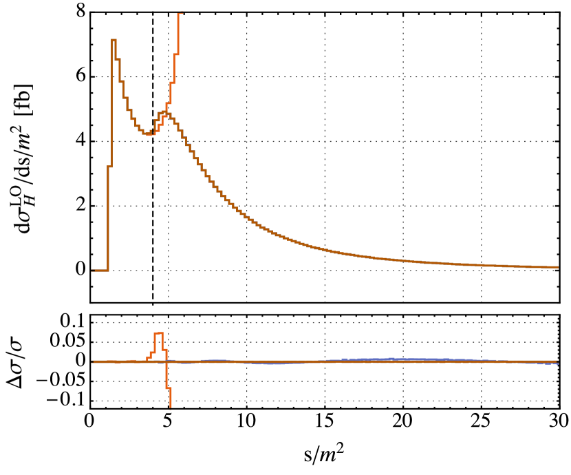
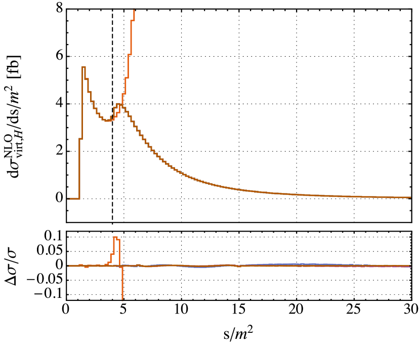
Figure 3: Left panel: Leading-order $gg\to H\to ZZ$ cross section. 1.) LME up to $1/m^{20}$ (orange). 2.) Exact result (black), LME with conformal mapping (blue) and Padé approximants $[4/4],[4/5],[5/4],[5/5]$ (yellow, purple, green, brown) agree perfectly. Right panel: Virtual NLO corrections to $gg\to H\to ZZ$ cross section. See text for details. Color code as in left panel. The bottom plots show the relative deviations with respect to the exact (N)LO results. The vertical dashed line denotes the top quark pair-production threshold.

The orange curves in Fig. 3 depict the large-mass expansion results of Eq. (32) for the LO and the NLO case, where each finite remainder ${\cal F}_{\cal A}^{(1,2)}$ is expanded up to $1/m^{20}$. A minimum cut $\sqrt{s}\geq 2m_{Z}$ has been imposed and the threshold for top quark pair-production is given by $s/m^{2}=4$. The relative deviation

$$\frac{\Delta\sigma}{\sigma}=1-\frac{\sigma^{\text{(N)LO}}_{\text{approx}}}{\sigma^{\text{(N)LO}}_{\text{exact}}}$$ (34)

of the approximated results with respect to the exact result are shown in the bottom plots. The large-mass expansion describes the exact LO and virtual NLO results up to the top threshold very well, with only $5\%$ deviation at LO and $7\%$ at NLO at $s=4m^{2}$. As expected however the large-mass expansion diverges for values above this threshold. Improvements to this naive approximation by means of the conformal mapping, Eq. (29), are shown in blue. On top we compute the diagonal, $[5/5]$ (brown) and $[4/4]$ (yellow), and non-diagonal, $[4/5]$ (purple) and $[5/4]$ (green), Padé approximants at amplitude level for the mapped series expressions of each finite remainder, i.e. ${\cal F}_{{\cal A},[n/m]}^{(i)}$. Both results, using the Padé approximants or the mapped series alone, excellently reproduce the exact results (black curve) even far above threshold; with less than $1\%$ deviation from the exact result over the considered range. As a result the Padé approximant $[5/5]$ overlays all other curves in Fig. 3, some of which are scarcely visible.

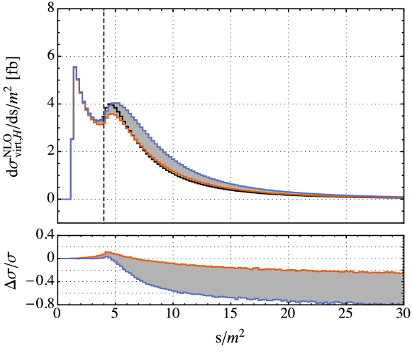
Figure 4: Virtual NLO corrections to $gg\to H\to ZZ$ cross section with rescaling from Eq. (26). See text for details. 1.) Exact NLO result (black). 2.) Varying orders of rescaled LMEs are indicated by shaded grey area. Its envelope is given by $\sigma_{\text{imp},1}^{\text{NLO}}$ (orange) and $\sigma_{\text{imp},10}^{\text{NLO}}$ (blue). The bottom plot shows the relative deviations with respect to the exact NLO results. The vertical dashed line denotes the top quark pair-production threshold.

The second choice of improving the naive LME is given by the rescaling from Eq. (26). The results are shown in Fig. 4. The exact virtual NLO result is again shown in black. The rescaled LMEs are indicated by the shaded grey area and its envelope is given by the expansions $\sigma_{\text{imp},1}^{\text{NLO}}$ (orange) and $\sigma_{\text{imp},10}^{\text{NLO}}$ (blue). Although the heavy-quark approximation $\sigma_{\text{imp},1}^{\text{NLO}}$ gives a reasonable estimate of the exact result above threshold it fails to describe the threshold behaviour and peak structure of the exact result. At threshold the deviation is $10\%$. Taking higher orders in the expansion into account improves the threshold prescription, with $3\%$ deviation for $\sigma_{\text{imp},10}^{\text{NLO}}$ at threshold, but worsens the trend for higher energies. In both cases we find more than $20\%$ deviation for $s/m^{2}>20$.

We end this section by drawing our conclusions from the results presented. We see that, at least in the single-scale Higgs boson production and having a sufficient number of terms in the LME at hand, applying the conformal mapping (and the Padé approximation) yields excellent prescriptions of the exact results. The conformal mapping is imperative, whereas the additional Padé approximants give only small improvements in terms of uncertainty reduction and stability of the approximations. We conclude that we should favour these approximations over the rescaling method.

One important point to notice, however, is that the kinematics change when moving from the single Higgs boson production to the SM $Z$ boson pair-production. Therefore, the results discussed here may not necessarily transfer easily. Still, the comparisons within this chapter should give an idea of the validity of the improved large-mass expansions. We will discuss analogous considerations for the Z boson pair-production in Sec. 3.5.

3 Virtual Corrections to SM $ZZ$ Production via Massive Quark Loops

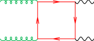
(a)

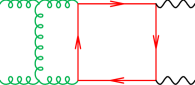
(b)

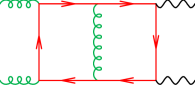
(c)

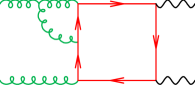
(d)

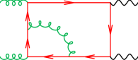
(e)

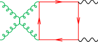
(f)

Figure 5: Representative diagrams for the LO and virtual NLO $gg\to ZZ$ amplitude.

After we set the stage in the previous chapters, including derivation of known results for the single Higgs amplitudes and extending their expansion to higher orders, we can now tackle the unknown QCD corrections to $Z$ boson pair-production via massive quark loops in the SM. Representative diagrams for the leading-order contribution are illustrated in Fig. 5(a) and for the virtual next-to-leading-order diagrams in Fig. 5(b)-(f) and Fig. 6, respectively.

These amplitudes were first studied for on-shell $Z$ bosons in Ref. Glover:1988rg ; more recently, the $Z$ decay and off-shell effects were also calculated at leading-order Campbell:2013una . Virtual two-loop contributions with massless internal quark loops (and subsequent $Z$ boson decay) became available only recentlyGehrmann:2014bfa ; Cascioli:2014yka ; Caola:2014iua ; Gehrmann:2015ora ; Caola:2015ila ; vonManteuffel:2015msa . Due to the complexity of the computation and present technical limitations no full two-loop correction to the amplitudes with massive internal quarks is presently known. The authors of Melnikov:2015laa made the first attempt in approximating the virtual NLO corrections with internal top quarks. Their results, however, includes only the first term of the $1/m$ expansion. At this order contributions from the vector coupling of the $Z$ bosons to the quarks are neglected completely. This is not necessarily troubling since the vector coupling contribution is $a_{f}/v_{f}\sim 2.5$ times smaller than the axial coupling contribution.

However, to fully incorporate the physics of the $Z$ boson interactions and to give an estimate of power corrections $s/m^{2}$ we compute the virtual two-loop corrections up to ${\cal O}\left(r_{t}^{-7}\right)$. We keep the $Z$ bosons on-shell, sum over their polarisations and project onto the tensor structure of the $gg\to H\to ZZ$ amplitude (Eq. (17)) since we are only interested in the interference of both.

This chapter is structured as follows: In Sec. 3.1 we give our definitions of the SM $ZZ$ amplitude, as far as the conventions differ from Sec. 2.1. The leading-order and next-to-leading-order results are presented in Sec. 3.3 and Sec. 3.4, respectively. The latter is divided into two parts; the first consists of diagrams where both $Z$ bosons couple to one fermion line and the second handles anomaly style diagrams where a single $Z$ boson is connected to one fermion string.

3.1 Preliminaries

The on-shell $Z$ boson pair-production in gluon-gluon fusion

$$g(p_{1},\mu,A)+g(p_{2},\nu,B)\to Z(p_{3},m_{Z},\alpha)+Z(p_{4},m_{Z},\beta)\,,$$ (35)

via the heavy top quark loop can be completely expressed in terms of kinematical invariants

$$p_{3}^{2}=m_{Z}^{2}=p_{4}^{2}\,,\quad s=(p_{1}+p_{2})^{2}\,,\quad t=(p_{1}-p_{3})^{2}\,,\quad u=(p_{2}-p_{3})^{2}\text{ and }\;s+t+u=2m_{Z}^{2}\,,$$ (36)

or equivalently, using the on-shellness condition, by the rescaled variables

$$r_{t} =\frac{m^{2}}{s}\,,\quad r_{Z}=\frac{m_{Z}^{2}}{s}\,,\quad x=\frac{m_{Z}^{2}-t}{s}=\frac{p_{1}p_{3}}{p_{1}p_{2}}\;\;\text{and}\;\;\tilde{x}=(1-x)x\,.$$ (37)

The SM continuum amplitudes $\ket{{\cal B}^{0,AB}_{\mu\nu\alpha\beta}(\alpha_{S}^{0},m^{0},\mu,\epsilon)}$ admit the same perturbative expansion as given in Eq. (3) for the Higgs-mediated process. The bare amplitudes are renormalized in accordance with Eqs. (5-14), omitting the superfluous Higgs vertex renormalisation. As mentioned earlier we project onto the tensor and color structure of the Higgs-mediated amplitude (Eq. (17)) with

$$\ket{{\cal B}^{0}(\alpha_{S}^{0},m^{0},\mu,\epsilon)}=\frac{\delta^{AB}}{N_{A}}(g^{\mu\nu}\,p_{1}p_{2}-p_{2}^{\mu}p_{1}^{\nu})\;P_{Z}^{\alpha\rho^{\prime}}(p_{3})P_{Z,\rho^{\prime}}^{\beta}(p_{4})\ket{{\cal B}^{0,AB}_{\mu\nu\alpha\beta}(\alpha_{S}^{0},m^{0},\mu,\epsilon)}\,,$$ (38)

where $N_{A}=N_{c}^{2}-1=8$ and $P_{Z,\alpha\beta}(p)$ from Eq. (19).
We shall consider a single quark of flavor $f$ to be circulating in the quark loop. The Standard Model coupling of this fermion to a $Z$ boson is given by,

$$-i\frac{g_{W}}{2\cos\theta_{W}}\gamma^{\mu}\left(v_{f}-a_{f}\gamma_{5}\right),\;\;v_{f}=\tau_{f}-2Q_{f}\sin^{2}\theta_{W},\;\;a_{f}=\tau_{f},\;\;\tau_{f}=\pm\frac{1}{2}\,.$$ (39)

The superposition of vector and axial coupling allows to write the scattering amplitude as

$$\ket{{\cal B}^{0}(\alpha_{S}^{0},m^{0},\mu,\epsilon)}={\cal N}\;\left(v_{f}^{2}\ket{\widetilde{{\cal B}}_{VV}^{0}(\alpha_{S}^{0},m^{0},\mu,\epsilon)}+a_{f}^{2}\ket{\widetilde{{\cal B}}_{AA}^{0}(\alpha_{S}^{0},m^{0},\mu,\epsilon)}\right)\,,$$ (40)

where we factored out the normalisation factor from Eq. (18). The mixed coupling structure $v_{f}a_{f}$ vanishes due to charge parity conservation. With the amplitudes outlined above it is straightforward to compute the interference.

$${\cal B}_{gg} =2{\rm Re}\Bigl{\{}\bra{{\cal A}_{\alpha\beta\rho^{\prime}\sigma^{\prime}}^{AB}(\alpha_{S}^{(n_{l})},m,\mu,\epsilon)}\ket{{\cal B}^{AB,\alpha\beta\rho\sigma}(\alpha_{S}^{(n_{l})},m,\mu,\epsilon)}\;P^{\rho^{\prime}}_{Z,\rho}(p_{3})P^{\sigma^{\prime}}_{Z,\sigma}(p_{4})\Bigl{\}}$$

$$=2{\rm Re}\Bigl{\{}{\cal N}^{*}\frac{8}{3}\frac{s\,N_{A}}{s-m_{H}^{2}}\bra{{\cal A}(\alpha_{S}^{(n_{l})},m,\mu,\epsilon)}\ket{{\cal B}(\alpha_{S}^{(n_{l})},m,\mu,\epsilon)}\Bigl{\}}$$ (41)

$$=|{\cal N}|^{2}\frac{16}{3}\frac{s\,N_{A}}{s-m_{H}^{2}}\;{\rm Re}\Bigl{\{}\bra{{\cal A}(\alpha_{S}^{(n_{l})},m,\mu,\epsilon)}\left[v_{f}^{2}\ket{\widetilde{{\cal B}}_{VV}(\alpha_{S}^{(n_{l})},m,\mu,\epsilon)}+a_{f}^{2}\ket{\widetilde{{\cal B}}_{AA}(\alpha_{S}^{(n_{l})},m,\mu,\epsilon)}\right]\Bigl{\}}\,.$$

Writing Eq. (3.1) in this way establishes that ${\cal A}(\alpha_{S}^{(n_{l})},m,\mu,\epsilon)$ and ${\cal B}(\alpha_{S}^{(n_{l})},m,\mu,\epsilon)$ are dimensionless quantities, i.e. we compute ${\cal B}(\alpha_{S}^{(n_{l})},m,\mu,\epsilon)$ for $s=1$ in the following.

3.2 Projected Exact Result at One Loop

The leading-order amplitude for the SM continuum production of two $Z$ bosons is known exactly in $d=4-2\epsilon$ dimensions. The usual normalisation factor Eq. (22) is chosen. We split the result, according to Eq. (40), into vector-vector ($VV$) and axial-axial ($AA$) contribution.

$$\ket{\widetilde{{\cal B}}_{VV}^{(1)}(r_{t},\mu,\epsilon)} =S_{\epsilon}\,c_{\Gamma}\cdot 2\Big{\{}4\epsilon(1-\epsilon)B_{\{1,2\}}+2\epsilon\left(B_{\{1,3\}}+B_{\{2,3\}}-2B_{\{3\}}\right)$$ (42)

$$+sC_{\{1,2\}}\left[8r_{t}+2\epsilon(1-4r_{t})-2\epsilon^{2}\right]+sC_{\{23,1\}}\left[2(1-4r_{t}-2r_{Z})(1-x)-4\epsilon(1-r_{Z})(1-x)\right]$$

$$+sC_{\{12,3\}}\left[\epsilon\left(2(1-4r_{t}-2r_{Z})-2\epsilon(1-2r_{Z})\right)\right]+sC_{\{1,3\}}\left[2(1-4r_{t}-2r_{Z})x-4\epsilon(1-r_{Z})x\right]$$

$$+s^{2}D_{\{1,2,3\}}\left[4r_{t}(1-2r_{t}-r_{Z})+\epsilon\left((1-4r_{t})(1-r_{Z})-x\right)+\epsilon^{2}\left(-1+r_{Z}+x\right)\right]$$

$$+s^{2}D_{\{2,1,3\}}\left[4r_{t}(1-2r_{t}-r_{Z})+\epsilon\left(4r_{t}(-1+r_{Z})-r_{Z}+x\right)+\epsilon^{2}\left(r_{Z}-x\right)\right]$$

$$+s^{2}D_{\{1,3,2\}}\left[(1-4r_{t}-2r_{Z})\left(2r_{t}-r_{Z}+x-x^{2}\right)+\epsilon\left(4r_{t}(-1+r_{Z})+(1-2r_{Z})(r_{Z}-(1-x)x)\right)\right.$$

$$+\left.\epsilon^{2}\left(r_{Z}-(1-x)x\right)\right]\Big{\}}\,.$$

$$\ket{\widetilde{{\cal B}}_{AA}^{(1)}(r_{t},\mu,\epsilon)} =\ket{\widetilde{{\cal B}}_{VV}^{(1)}(r_{t},\mu,\epsilon)}+S_{\epsilon}\,c_{\Gamma}\cdot 2r_{t}\Big{\{}sC_{\{1,2\}}\left[(2-4r_{Z})/r_{Z}^{2}\right]$$ (43)

$$+sC_{\{23,1\}}\left[4(1-6r_{Z})(-1+x)/r_{Z}-16\epsilon(1-x)\right]+sC_{\{12,3\}}\left[\epsilon\left(24+(2-8r_{Z})/r_{Z}^{2}-16\epsilon\right)\right]$$

$$+sC_{\{1,3\}}\left[4\left(6-1/r_{Z}\right)x-16\epsilon x\right]$$

$$+s^{2}D_{\{1,2,3\}}\left[-4+24r_{t}+2r_{t}/r_{Z}^{2}-8r_{t}/r_{Z}+\epsilon\left(10-16r_{t}+(1-x)/r_{Z}^{2}-(3-2x)/r_{Z}\right)-4\epsilon^{2}\right]$$

$$+s^{2}D_{\{2,1,3\}}\left[-4+24r_{t}+2r_{t}/r_{Z}^{2}-8r_{t}/r_{Z}+\epsilon\left(10-16r_{t}-(1+2x)/r_{Z}+x/r_{Z}^{2}\right)-4\epsilon^{2}\right]$$

$$+s^{2}D_{\{1,3,2\}}\left[2r_{t}/r_{Z}^{2}-12r_{Z}-(8r_{t}+2(1-x)x)/r_{Z}+2\ \left(1+12r_{t}+6x-6x^{2}\right)\right.$$

$$+\left.\epsilon\left(8r_{Z}-2\left(8r_{t}-(1-2x)^{2}\right)+(1-x)x/r_{Z}^{2}-(1-2x+2x^{2})/r_{Z}\right)-4\epsilon^{2}\right]\Big{\}}\,.$$

The notation for the scalar integrals $B,C$ and $D$ is given in Table 1.

$D_{\{1,2,3\}}$	$D_{0}(q_{1},q_{2},q_{3};m,m,m,m)$	$C_{\{1,2\}}$	$C_{0}(q_{1},q_{2};m,m,m)$	$B_{\{1,2\}}$	$B_{0}(q_{12};m,m)$
$D_{\{1,3,2\}}$	$D_{0}(q_{1},q_{3},q_{2};m,m,m,m)$	$C_{\{1,3\}}$	$C_{0}(q_{1},q_{3};m,m,m)$	$B_{\{1,3\}}$	$B_{0}(q_{13};m,m)$
$D_{\{2,1,3\}}$	$D_{0}(q_{2},q_{1},q_{3};m,m,m,m)$	$C_{\{12,3\}}$	$C_{0}(q_{12},q_{3};m,m,m)$	$B_{\{2,3\}}$	$B_{0}(q_{23};m,m)$
		$C_{\{23,1\}}$	$C_{0}(q_{23},q_{1};m,m,m)$	$B_{\{3\}}$	$B_{0}(q_{3};m,m)$

Table 1: Scalar integrals occurring in full LO SM continuum $ZZ$ production. The momenta are defined as $q_{1}=p_{1},q_{2}=p_{2},q_{3}=-p_{3}$ and $q_{ij}=q_{i}+q_{j}$. The scalar integrals are defined in appendix A.

We re-introduced factors of $s$ in Eq. (42) and Eq. (43) to indicate the correct dimensionality of the expressions. We note that, in contrast to the case where the $Z$ bosons are off-shell and their decays included, these formulae for the interference take a very simple form. Eq. (42,43) extend the results of Ref Campbell:2014gua to include the terms of order $\epsilon^{1}$ and $\epsilon^{2}$.

3.3 Large-Mass Expansion at One Loop

Equivalently, Eq. (42) and Eq. (43) can be expressed by means of the large-mass expansion. The result for the vector-vector part yields

$$\ket{\widetilde{{\cal B}}_{VV}^{(1)}(r_{t},\mu,\epsilon)} =S_{\epsilon}\,c_{\Gamma}\,\left(\frac{\mu^{2}}{m^{2}}\right)^{\epsilon}\Bigg{\{}\frac{1}{r_{t}^{2}}\left[\frac{1}{10}-\frac{r_{Z}}{5}+\epsilon^{2}\left(-\frac{1}{10}+\frac{4r_{Z}}{15}-\frac{\tilde{x}}{15}\right)+\epsilon\left(\frac{1}{15}-\frac{17r_{Z}}{45}+\frac{11\tilde{x}}{45}\right)\right]$$

$$+\frac{1}{r_{t}^{3}}\left[\frac{2}{315}+\frac{r_{Z}}{21}-\frac{4r_{Z}^{2}}{35}-\frac{4\tilde{x}}{315}+\epsilon^{2}\left(-\frac{4}{315}-\frac{149r_{Z}}{3780}+\frac{17r_{Z}^{2}}{315}+\left(\frac{143}{3780}+\frac{2r_{Z}}{45}\right)\tilde{x}\right)\right.$$

$$+\left.\epsilon\left(-\frac{1}{105}+\frac{61r_{Z}}{945}-\frac{68r_{Z}^{2}}{315}+\left(\frac{37}{1890}+\frac{8r_{Z}}{63}\right)\tilde{x}\right)\right]+\frac{1}{r_{t}^{4}}\left[\frac{1}{1080}-\frac{r_{Z}}{1260}+\frac{41r_{Z}^{2}}{1890}-\frac{r_{Z}^{3}}{21}\right.$$

$$+\left(\frac{1}{945}-\frac{2r_{Z}}{315}\right)\tilde{x}+\epsilon\left(\frac{131}{45360}-\frac{61r_{Z}}{4200}+\frac{2171r_{Z}^{2}}{56700}-\frac{59r_{Z}^{3}}{630}+\left(-\frac{47}{28350}+\frac{319r_{Z}}{18900}+\frac{16r_{Z}^{2}}{315}\right)\tilde{x}\right.$$

$$-\left.\left.\frac{13\tilde{x}^{2}}{2700}\right)+\epsilon^{2}\left(\frac{1}{1008}-\frac{31r_{Z}}{3240}-\frac{7r_{Z}^{2}}{810}-\frac{2r_{Z}^{3}}{945}+\left(-\frac{7}{1620}+\frac{659r_{Z}}{22680}+\frac{37r_{Z}^{2}}{945}\right)\tilde{x}-\frac{43\tilde{x}^{2}}{22680}\right)\right]$$

$$+\frac{1}{r_{t}^{5}}\left[\frac{4}{17325}+\frac{r_{Z}}{2475}-\frac{43r_{Z}^{2}}{20790}+\frac{r_{Z}^{3}}{110}-\frac{4r_{Z}^{4}}{231}+\left(-\frac{1}{2079}+\frac{13r_{Z}}{20790}-\frac{r_{Z}^{2}}{693}\right)\tilde{x}+\frac{\tilde{x}^{2}}{2310}\right.$$ (44)

$$+\epsilon\left(-\frac{1}{4725}+\frac{r_{Z}}{330}-\frac{2671r_{Z}^{2}}{249480}+\frac{2533r_{Z}^{3}}{138600}-\frac{53r_{Z}^{4}}{1485}+\left(\frac{349}{311850}-\frac{733r_{Z}}{178200}+\frac{67r_{Z}^{2}}{5940}+\frac{188r_{Z}^{3}}{10395}\right)\tilde{x}\right.$$

$$+\left.\left(\frac{37}{59400}-\frac{4r_{Z}}{825}\right)\tilde{x}^{2}\right)+\epsilon^{2}\left(-\frac{67}{103950}+\frac{73r_{Z}}{32400}-\frac{16871r_{Z}^{2}}{2494800}+\frac{323r_{Z}^{3}}{831600}-\frac{67r_{Z}^{4}}{8910}\right.$$

$$+\left.\left.\left(\frac{5939}{2494800}-\frac{451r_{Z}}{75600}+\frac{839r_{Z}^{2}}{51975}+\frac{611r_{Z}^{3}}{31185}\right)\tilde{x}+\left(-\frac{2083}{2494800}-\frac{61r_{Z}}{17325}\right)\tilde{x}^{2}\right)\right]$$

$$+\frac{1}{r_{t}^{6}}\left[\frac{1}{108108}+\frac{5r_{Z}}{54054}+\frac{569r_{Z}^{2}}{1801800}-\frac{163r_{Z}^{3}}{108108}+\frac{7r_{Z}^{4}}{1980}-\frac{5r_{Z}^{5}}{858}+\left(\frac{1}{9009}-\frac{19r_{Z}}{42900}-\frac{r_{Z}^{2}}{90090}+\frac{4r_{Z}^{3}}{19305}\right)\tilde{x}\right.$$

$$+\left(-\frac{97}{600600}+\frac{29r_{Z}}{60060}\right)\tilde{x}^{2}+\epsilon^{2}\left(\frac{191}{1853280}-\frac{28507r_{Z}}{32432400}+\frac{444149r_{Z}^{2}}{216216000}-\frac{263839r_{Z}^{3}}{64864800}+\frac{301471r_{Z}^{4}}{194594400}\right.$$

$$-\frac{5743r_{Z}^{5}}{1297296}+\left(-\frac{8269}{16216200}+\frac{82241r_{Z}}{24948000}-\frac{23113r_{Z}^{2}}{4633200}+\frac{11041r_{Z}^{3}}{1389960}+\frac{5185r_{Z}^{4}}{648648}\right)\tilde{x}+\frac{46\tilde{x}^{3}}{405405}$$

$$+\left.\left(\frac{98009}{216216000}-\frac{58703r_{Z}}{64864800}-\frac{9979r_{Z}^{2}}{3243240}\right)\tilde{x}^{2}\right)+\epsilon\left(\frac{617}{6486480}-\frac{13037r_{Z}}{22702680}+\frac{1785391r_{Z}^{2}}{756756000}-\frac{274301r_{Z}^{3}}{45405360}\right.$$

$$+\frac{19199r_{Z}^{4}}{2494800}-\frac{19r_{Z}^{5}}{1512}+\left(-\frac{53}{291060}+\frac{60449r_{Z}}{34398000}-\frac{153919r_{Z}^{2}}{37837800}+\frac{137r_{Z}^{3}}{21450}+\frac{25r_{Z}^{4}}{4158}\right)\tilde{x}$$

$$+\left.\left.\left(-\frac{1091}{19404000}+\frac{47153r_{Z}}{75675600}-\frac{167r_{Z}^{2}}{54054}\right)\tilde{x}^{2}+\frac{29\tilde{x}^{3}}{189189}\right)\right]+{\cal O}\left(1/r_{t}^{7},\epsilon^{3}\right)\Bigg{\}}\,.$$

The result for the axial-axial part is

$$\ket{\widetilde{{\cal B}}_{AA}^{(1)}(r_{t},\mu,\epsilon)} =S_{\epsilon}\,c_{\Gamma}\,\left(\frac{\mu^{2}}{m^{2}}\right)^{\epsilon}\Bigg{\{}\frac{1}{r_{t}}\left[-2-\frac{1}{6r_{Z}^{2}}+\frac{2}{3r_{Z}}+\epsilon^{2}\left(\frac{4}{3}+\frac{1}{6r_{Z}^{2}}-\frac{1}{r_{Z}}+\left(\frac{1}{3r_{Z}^{2}}+\frac{2}{3r_{Z}}\right)\tilde{x}\right)\right.$$

$$+\left.\epsilon\left(2-\frac{1}{3r_{Z}}+\left(\frac{1}{3r_{Z}^{2}}+\frac{2}{3r_{Z}}\right)\tilde{x}\right)\right]+\frac{1}{r_{t}^{2}}\left[\frac{7}{30}+\frac{1}{90r_{Z}^{2}}-\frac{7}{90r_{Z}}-\frac{3r_{Z}}{5}+\left(-\frac{1}{30r_{Z}^{2}}+\frac{1}{15r_{Z}}\right)\tilde{x}\right.$$

$$+\epsilon^{2}\left(-\frac{31}{90}-\frac{1}{90r_{Z}^{2}}+\frac{17}{180r_{Z}}+\frac{7r_{Z}}{9}+\left(\frac{2}{9}+\frac{1}{60r_{Z}^{2}}\right)\tilde{x}\right)+\epsilon\left(\frac{1}{180r_{Z}^{2}}-\frac{1}{36r_{Z}}+\frac{4r_{Z}}{45}\right.$$ (45)

$$+\left.\left.\left(\frac{17}{45}-\frac{1}{36r_{Z}^{2}}+\frac{7}{90r_{Z}}\right)\tilde{x}\right)\right]+\frac{1}{r_{t}^{3}}\left[-\frac{13}{210}-\frac{1}{280r_{Z}^{2}}+\frac{13}{630r_{Z}}+\frac{2r_{Z}}{21}-\frac{6r_{Z}^{2}}{35}+\left(\frac{4}{63}+\frac{1}{126r_{Z}^{2}}\right.\right.$$

$$-\left.\frac{13}{315r_{Z}}\right)\tilde{x}+\epsilon^{2}\left(\frac{149}{1890}+\frac{1}{336r_{Z}^{2}}-\frac{403}{15120r_{Z}}-\frac{2r_{Z}}{15}+\frac{23r_{Z}^{2}}{105}+\left(-\frac{71}{1260}+\frac{43}{15120r_{Z}^{2}}+\frac{337}{7560r_{Z}}\right.\right.$$

$$+\left.\left.\frac{32r_{Z}}{315}\right)\tilde{x}+\left(-\frac{11}{840r_{Z}^{2}}-\frac{11}{420r_{Z}}\right)\tilde{x}^{2}\right)+\epsilon\left(-\frac{101}{3780}-\frac{1}{336r_{Z}^{2}}+\frac{13}{1080r_{Z}}+\frac{4r_{Z}}{135}-\frac{17r_{Z}^{2}}{315}\right.$$

$$+\left.\left.\left(\frac{73}{1890}+\frac{89}{7560r_{Z}^{2}}-\frac{109}{3780r_{Z}}+\frac{8r_{Z}}{63}\right)\tilde{x}+\left(-\frac{1}{140r_{Z}^{2}}-\frac{1}{70r_{Z}}\right)\tilde{x}^{2}\right)\right]+\frac{1}{r_{t}^{4}}\left[\frac{517}{37800}+\frac{2}{4725r_{Z}^{2}}\right.$$

$$-\frac{2}{525r_{Z}}-\frac{13r_{Z}}{420}+\frac{13r_{Z}^{2}}{378}-\frac{r_{Z}^{3}}{21}+\left(-\frac{32}{945}-\frac{2}{945r_{Z}^{2}}+\frac{4}{315r_{Z}}+\frac{4r_{Z}}{105}\right)\tilde{x}+\left(\frac{1}{945r_{Z}^{2}}-\frac{2}{945r_{Z}}\right)\tilde{x}^{2}$$

$$+\epsilon\left(\frac{127}{11340}+\frac{13}{28350r_{Z}^{2}}-\frac{1}{270r_{Z}}-\frac{23r_{Z}}{1050}+\frac{1163r_{Z}^{2}}{56700}-\frac{19r_{Z}^{3}}{630}+\left(-\frac{257}{11340}-\frac{11}{4050r_{Z}^{2}}+\frac{19}{1350r_{Z}}\right.\right.$$

$$+\left.\left.\frac{71r_{Z}}{2700}+\frac{4r_{Z}^{2}}{105}\right)\tilde{x}+\left(-\frac{283}{18900}+\frac{167}{56700r_{Z}^{2}}-\frac{17}{4050r_{Z}}\right)\tilde{x}^{2}\right)+\epsilon^{2}\left(-\frac{6829}{453600}-\frac{1}{3780r_{Z}^{2}}+\frac{37}{11340r_{Z}}\right.$$

$$+\frac{863r_{Z}}{25200}-\frac{811r_{Z}^{2}}{18900}+\frac{17r_{Z}^{3}}{315}+\left(\frac{568}{14175}+\frac{1}{2268r_{Z}^{2}}-\frac{11}{1512r_{Z}}-\frac{4157r_{Z}}{113400}+\frac{4r_{Z}^{2}}{105}\right)\tilde{x}$$

$$+\left.\left.\left(-\frac{401}{16200}+\frac{1}{324r_{Z}^{2}}-\frac{1}{378r_{Z}}\right)\tilde{x}^{2}\right)\right]+\frac{1}{r_{t}^{5}}\left[-\frac{767}{207900}-\frac{1}{8316r_{Z}^{2}}+\frac{13}{13860r_{Z}}+\frac{1699r_{Z}}{207900}-\frac{31r_{Z}^{2}}{2310}\right.$$

$$+\frac{8r_{Z}^{3}}{693}-\frac{r_{Z}^{4}}{77}+\left(\frac{83}{6930}+\frac{1}{1980r_{Z}^{2}}-\frac{13}{3465r_{Z}}-\frac{437r_{Z}}{20790}+\frac{r_{Z}^{2}}{55}\right)\tilde{x}+\left(-\frac{1}{315}-\frac{1}{1980r_{Z}^{2}}+\frac{1}{420r_{Z}}\right)\tilde{x}^{2}$$

$$+\epsilon\left(-\frac{9299}{2494800}-\frac{1}{6480r_{Z}^{2}}+\frac{871}{831600r_{Z}}+\frac{19651r_{Z}}{2494800}-\frac{5209r_{Z}^{2}}{415800}+\frac{167r_{Z}^{3}}{17325}-\frac{43r_{Z}^{4}}{3780}+\left(\frac{5323}{415800}+\frac{223}{277200r_{Z}^{2}}\right.\right.$$

$$-\left.\frac{244}{51975r_{Z}}-\frac{21121r_{Z}}{1247400}+\frac{3271r_{Z}^{2}}{207900}+\frac{113r_{Z}^{3}}{10395}\right)\tilde{x}+\left(-\frac{383}{207900}-\frac{313}{277200r_{Z}^{2}}+\frac{349}{92400r_{Z}}-\frac{53r_{Z}}{5775}\right)\tilde{x}^{2}$$

$$+\left.\left(\frac{1}{4158r_{Z}^{2}}+\frac{1}{2079r_{Z}}\right)\tilde{x}^{3}\right)+\epsilon^{2}\left(\frac{16273}{4989600}+\frac{7}{142560r_{Z}^{2}}-\frac{923}{1247400r_{Z}}-\frac{3497r_{Z}}{453600}+\frac{30463r_{Z}^{2}}{2494800}\right.$$

$$-\frac{305r_{Z}^{3}}{24948}+\frac{3089r_{Z}^{4}}{249480}+\left(-\frac{1493}{166320}+\frac{47}{311850r_{Z}^{2}}+\frac{4507}{2494800r_{Z}}+\frac{5191r_{Z}}{226800}-\frac{19627r_{Z}^{2}}{1247400}+\frac{227r_{Z}^{3}}{17820}\right)\tilde{x}$$

$$+\left.\left.\left(\frac{5161}{1247400}-\frac{4451}{4989600r_{Z}^{2}}+\frac{1123}{1663200r_{Z}}-\frac{3187r_{Z}}{207900}\right)\tilde{x}^{2}+\left(\frac{137}{249480r_{Z}^{2}}+\frac{137}{124740r_{Z}}\right)\tilde{x}^{3}\right)\right]$$

$$+\frac{1}{r_{t}^{6}}\left[\frac{2603}{2910600}+\frac{1}{56056r_{Z}^{2}}-\frac{1}{5096r_{Z}}-\frac{1223r_{Z}}{491400}+\frac{22381r_{Z}^{2}}{5405400}-\frac{34r_{Z}^{3}}{6435}+\frac{19r_{Z}^{4}}{5148}-\frac{r_{Z}^{5}}{286}+\left(-\frac{1019}{257400}\right.\right.$$

$$-\left.\frac{1}{8008r_{Z}^{2}}+\frac{941}{900900r_{Z}}+\frac{11447r_{Z}}{1351350}-\frac{5897r_{Z}^{2}}{540540}+\frac{293r_{Z}^{3}}{38610}\right)\tilde{x}+\left(\frac{5167}{1801800}+\frac{167}{900900r_{Z}^{2}}-\frac{697}{600600r_{Z}}\right.$$

$$-\left.\frac{493r_{Z}}{180180}\right)\tilde{x}^{2}+\left(-\frac{1}{24024r_{Z}^{2}}+\frac{1}{12012r_{Z}}\right)\tilde{x}^{3}+\epsilon^{2}\left(-\frac{50693}{87318000}-\frac{1}{288288r_{Z}^{2}}+\frac{59}{720720r_{Z}}\right.$$

$$+\frac{2049041r_{Z}}{1135134000}-\frac{3861083r_{Z}^{2}}{1238328000}+\frac{5078077r_{Z}^{3}}{1362160800}-\frac{616361r_{Z}^{4}}{194594400}+\frac{17341r_{Z}^{5}}{6486480}+\left(\frac{863221}{378378000}-\frac{1}{51480r_{Z}^{2}}\right.$$

$$-\left.\frac{2159}{11583000r_{Z}}-\frac{41229697r_{Z}}{6810804000}+\frac{6865009r_{Z}^{2}}{681080400}-\frac{26227r_{Z}^{3}}{4864860}+\frac{12911r_{Z}^{4}}{3243240}\right)\tilde{x}+\left(-\frac{651821}{412776000}+\frac{2917}{11583000r_{Z}^{2}}\right.$$

$$-\left.\left.\frac{1741}{3861000r_{Z}}+\frac{162983r_{Z}}{34927200}-\frac{24883r_{Z}^{2}}{3243240}\right)\tilde{x}^{2}+\left(\frac{36731}{22702680}-\frac{43}{154440r_{Z}^{2}}+\frac{1}{5616r_{Z}}\right)\tilde{x}^{3}\right)$$

$$+\epsilon\left(\frac{2523253}{2270268000}+\frac{29}{1121120r_{Z}^{2}}-\frac{23}{86240r_{Z}}-\frac{932231r_{Z}}{324324000}+\frac{503059r_{Z}^{2}}{108108000}-\frac{674147r_{Z}^{3}}{113513400}+\frac{3541r_{Z}^{4}}{926640}\right.$$

$$-\frac{4051r_{Z}^{5}}{1081080}+\left(-\frac{3717937}{756756000}-\frac{223}{1121120r_{Z}^{2}}+\frac{63961}{42042000r_{Z}}+\frac{908203r_{Z}}{94594500}-\frac{802811r_{Z}^{2}}{75675600}+\frac{3889r_{Z}^{3}}{491400}\right.$$

$$+\left.\frac{163r_{Z}^{4}}{54054}\right)\tilde{x}+\left(\frac{862991}{252252000}+\frac{48721}{126126000r_{Z}^{2}}-\frac{164711}{84084000r_{Z}}-\frac{7159r_{Z}}{5821200}-\frac{239r_{Z}^{2}}{54054}\right)\tilde{x}^{2}$$

$$+\left.\left.\left(\frac{283}{378378}-\frac{1789}{10090080r_{Z}^{2}}+\frac{1009}{5045040r_{Z}}\right)\tilde{x}^{3}\right)\right]+{\cal O}\left(1/r_{t}^{7},\epsilon^{3}\right)\Bigg{\}}\,.$$

The leading term in the vector-vector expansion is sub-dominant with respect to the axial-axial part. The reason for this difference has been given in Melnikov:2015laa .

3.4 Large-Mass Expansion at Two Loops

The two-loop SM continuum amplitude consists in total of $93+16$ non-zero diagrams. $93$ diagrams belong to topologies where both $Z$ bosons couple to the same fermion string, as illustrated in Fig. 5. Due to momentum conservation and assuming an anti-commuting $\gamma_{5}$ in $d$-dimensions, no $\gamma_{5}$ contribution arises in the fermion traces of the respective diagrams. The large-mass expansion results for the vector-vector and axial-axial part of these diagrams are shown in Sec. 3.4.1.

The remaining $16$ anomaly style diagrams belong to the topology shown in Fig. 6, where the $Z$ bosons couple to distinct fermion lines. These diagrams must, in principle, be handled with care when using dimensional regularisation due to the non-conservation of the axial-current. Furthermore, contributions from each quark-doublet have to be considered simultaneously. Only the sum over one quark-doublet leads to a gauge anomaly free theory. In case of massless quark doublets all contributions vanish and we only have to consider the third-generation quark doublet, i.e. top and bottom quarks. Results for these diagrams are presented in Sec. 3.4.2.

3.4.1 Non-Anomalous Diagrams

In this section we give explicit formulae for the large-mass expansions for the sum of the $93$ anomaly free diagrams. Including again only mass renormalisation, setting $\ket{\bar{{\cal B}}_{XX}^{(1)}(r_{t},\mu,\epsilon)}=\left(S_{\epsilon}c_{\Gamma}\,(\mu^{2}/m^{2})^{\epsilon}\,\right)^{-1}\ket{\widetilde{{\cal B}}_{XX}^{(1)}(r_{t},\mu,\epsilon)}$ and $\log(-r_{t})=\log(m^{2}/(-s-i\epsilon))$, we can write the divergent two-loop $VV$ part as

$$\ket{\widetilde{{\cal B}}_{VV}^{(2)}(r_{t},\mu,\epsilon)} =\left(S_{\epsilon}\,c_{\Gamma}\,\left(\frac{\mu^{2}}{m^{2}}\right)^{\epsilon}\right)^{2}\Bigg{\{}C_{A}\Bigg{[}\left(-\frac{2}{\epsilon^{2}}\left(\frac{m^{2}}{-s-i\epsilon}\right)^{\epsilon}+\frac{\pi^{2}}{3}\right)\ket{\bar{{\cal B}}_{VV}^{(1)}(r_{t},\mu,\epsilon)}$$

$$+\frac{1}{r_{t}^{2}}\left[\frac{251}{540}-\frac{317r_{Z}}{270}-\frac{11\tilde{x}}{135}\right]+\frac{1}{r_{t}^{3}}\left[-\frac{158129}{1587600}+\frac{127817r_{Z}}{396900}-\frac{5563r_{Z}^{2}}{9450}+\left(\frac{22558}{99225}-\frac{8r_{Z}}{189}\right)\tilde{x}\right.$$

$$+\left.\log(-r_{t})\left(-\frac{4}{315}-\frac{8r_{Z}}{315}+\frac{8\tilde{x}}{105}\right)\right]+\frac{1}{r_{t}^{4}}\left[\frac{132779}{9525600}-\frac{10421r_{Z}}{119070}+\frac{4411999r_{Z}^{2}}{23814000}-\frac{14521r_{Z}^{3}}{66150}\right.$$

$$+\left.\left(-\frac{252937}{5953500}+\frac{260483r_{Z}}{1701000}-\frac{16r_{Z}^{2}}{945}\right)\tilde{x}+\frac{13\tilde{x}^{2}}{20250}+\log(-r_{t})\left(\frac{1}{945}-\frac{4r_{Z}}{945}-\frac{4r_{Z}^{2}}{315}+\left(-\frac{2}{315}+\frac{4r_{Z}}{105}\right)\tilde{x}\right)\right]$$

$$+\frac{1}{r_{t}^{5}}\left[-\frac{19803283}{5762988000}+\frac{93293203r_{Z}}{5762988000}-\frac{61920091r_{Z}^{2}}{1152597600}+\frac{259936363r_{Z}^{3}}{2881494000}-\frac{236332r_{Z}^{4}}{3274425}+\left(\frac{3048977}{209563200}\right.\right.$$

$$-\left.\frac{55307339r_{Z}}{1280664000}+\frac{4889447r_{Z}^{2}}{68607000}-\frac{188r_{Z}^{3}}{31185}\right)\tilde{x}+\left(-\frac{32556823}{2881494000}+\frac{8r_{Z}}{12375}\right)\tilde{x}^{2}+\log(-r_{t})\left(-\frac{17}{41580}\right.$$

$$-\left.\left.\frac{r_{Z}}{2970}+\frac{r_{Z}^{2}}{4158}-\frac{2r_{Z}^{3}}{693}+\left(\frac{1}{315}-\frac{2r_{Z}}{693}+\frac{2r_{Z}^{2}}{231}\right)\tilde{x}-\frac{5\tilde{x}^{2}}{1386}\right)\right]+\frac{1}{r_{t}^{6}}\left[\frac{132076261729}{204528444120000}\right.$$ (46)

$$-\frac{857498948879r_{Z}}{204528444120000}+\frac{16366567901r_{Z}^{2}}{1377295920000}-\frac{1148974648051r_{Z}^{3}}{40905688824000}+\frac{22637379733r_{Z}^{4}}{584366983200}-\frac{165500519r_{Z}^{5}}{7491884400}$$

$$+\left(-\frac{101592736891}{25566055515000}+\frac{32900707079r_{Z}}{1826146822500}-\frac{57230507981r_{Z}^{2}}{2065943880000}+\frac{2366153189r_{Z}^{3}}{83480997600}-\frac{25r_{Z}^{4}}{12474}\right)\tilde{x}$$

$$+\left(\frac{341063392349}{68176148040000}-\frac{1401690458627r_{Z}}{102264222060000}+\frac{167r_{Z}^{2}}{405405}\right)\tilde{x}^{2}-\frac{29\tilde{x}^{3}}{2648646}+\log(-r_{t})\left(\frac{101}{1201200}-\frac{23r_{Z}}{163800}\right.$$

$$-\left.\left.\frac{1907r_{Z}^{2}}{1801800}+\frac{361r_{Z}^{3}}{540540}+\frac{8r_{Z}^{4}}{19305}+\left(-\frac{697}{900900}+\frac{2393r_{Z}}{900900}+\frac{31r_{Z}^{2}}{30030}-\frac{8r_{Z}^{3}}{6435}\right)\tilde{x}+\left(\frac{97}{72072}-\frac{145r_{Z}}{36036}\right)\tilde{x}^{2}\right)\right]\Bigg{]}$$

$$+C_{F}\Bigg{[}\frac{1}{r_{t}^{2}}\left[\frac{83}{54}-\frac{83r_{Z}}{27}\right]+\frac{1}{r_{t}^{3}}\left[\frac{1271}{5400}+\frac{2297r_{Z}}{2700}-\frac{1627r_{Z}^{2}}{675}-\frac{841\tilde{x}}{2025}\right]+\frac{1}{r_{t}^{4}}\left[\frac{18997}{1587600}+\frac{46231r_{Z}}{793800}\right.$$

$$+\left.\frac{1859807r_{Z}^{2}}{3969000}-\frac{1516r_{Z}^{3}}{1225}+\left(\frac{42367}{567000}-\frac{11663r_{Z}}{36750}\right)\tilde{x}\right]+\frac{1}{r_{t}^{5}}\left[\frac{533671}{47628000}-\frac{41471r_{Z}}{5103000}-\frac{28573r_{Z}^{2}}{1984500}\right.$$

$$+\left.\frac{16657657r_{Z}^{3}}{71442000}-\frac{312829r_{Z}^{4}}{595350}+\left(-\frac{2963}{105840}+\frac{278843r_{Z}}{3572100}-\frac{833081r_{Z}^{2}}{5953500}\right)\tilde{x}+\frac{229471\tilde{x}^{2}}{11907000}\right]$$

$$+\frac{1}{r_{t}^{6}}\left[-\frac{100790441}{302556870000}+\frac{10415465807r_{Z}}{1210227480000}-\frac{2539049r_{Z}^{2}}{488980800}-\frac{3259592869r_{Z}^{3}}{121022748000}+\frac{904486537r_{Z}^{4}}{8644482000}\right.$$

$$-\frac{1175777r_{Z}^{5}}{5880600}+\left(\frac{3025021753}{403409160000}-\frac{513331337r_{Z}}{14407470000}+\frac{1216539691r_{Z}^{2}}{27505170000}-\frac{10216127r_{Z}^{3}}{246985200}\right)\tilde{x}$$

$$+\left.\left(-\frac{10969455173}{1210227480000}+\frac{3151546457r_{Z}}{121022748000}\right)\tilde{x}^{2}\right]\Bigg{]}+{\cal O}\left(1/r_{t}^{7},\epsilon\right)\Bigg{\}}\,.$$

And the $AA$ part as

$$\ket{\widetilde{{\cal B}}_{AA}^{(2)}(r_{t},\mu,\epsilon)} =\left(S_{\epsilon}\,c_{\Gamma}\,\left(\frac{\mu^{2}}{m^{2}}\right)^{\epsilon}\right)^{2}\Bigg{\{}C_{A}\Bigg{[}\left(-\frac{2}{\epsilon^{2}}\left(\frac{m^{2}}{-s-i\epsilon}\right)^{\epsilon}+\frac{\pi^{2}}{3}\right)\ket{\bar{{\cal B}}_{AA}^{(1)}(r_{t},\mu,\epsilon)}$$

$$+\frac{1}{r_{t}}\left[-6-\frac{5}{9r_{Z}^{2}}+\frac{25}{9r_{Z}}+\left(-\frac{1}{9r_{Z}^{2}}-\frac{2}{9r_{Z}}\right)\tilde{x}\right]+\frac{1}{r_{t}^{2}}\left[\frac{3563}{2700}-\frac{17}{450r_{Z}^{2}}-\frac{761}{2700r_{Z}}-\frac{367r_{Z}}{270}+\left(-\frac{17}{135}\right.\right.$$

$$+\left.\left.\frac{47}{108r_{Z}^{2}}-\frac{1127}{1350r_{Z}}\right)\tilde{x}+\log(-r_{t})\left(\frac{2}{15}-\frac{1}{30r_{Z}^{2}}+\left(\frac{1}{5r_{Z}^{2}}-\frac{2}{5r_{Z}}\right)\tilde{x}\right)\right]+\frac{1}{r_{t}^{3}}\left[-\frac{27023}{176400}+\frac{5}{294r_{Z}^{2}}\right.$$

$$-\frac{23623}{793800r_{Z}}+\frac{8062r_{Z}}{14175}-\frac{37r_{Z}^{2}}{135}+\left(-\frac{142847}{198450}-\frac{2419}{22050r_{Z}^{2}}+\frac{28793}{56700r_{Z}}-\frac{8r_{Z}}{189}\right)\tilde{x}+\left(\frac{1}{1050r_{Z}^{2}}\right.$$

$$+\left.\left.\frac{1}{525r_{Z}}\right)\tilde{x}^{2}+\log(-r_{t})\left(-\frac{2}{105}+\frac{1}{126r_{Z}^{2}}-\frac{8}{315r_{Z}}+\frac{8r_{Z}}{63}+\left(-\frac{8}{21}-\frac{1}{21r_{Z}^{2}}+\frac{26}{105r_{Z}}\right)\tilde{x}\right)\right]$$

$$+\frac{1}{r_{t}^{4}}\left[-\frac{60007}{4762800}-\frac{1322471}{285768000r_{Z}^{2}}+\frac{2690033}{142884000r_{Z}}-\frac{100241r_{Z}}{1190700}+\frac{5018071r_{Z}^{2}}{23814000}-\frac{101r_{Z}^{3}}{2100}\right.$$ (47)

$$+\left(\frac{312127}{793800}+\frac{321799}{10206000r_{Z}^{2}}-\frac{736874}{4465125r_{Z}}-\frac{1195489r_{Z}}{2976750}-\frac{4r_{Z}^{2}}{315}\right)\tilde{x}+\left(\frac{283}{141750}-\frac{609137}{28576800r_{Z}^{2}}\right.$$

$$+\left.\frac{2876437}{71442000r_{Z}}\right)\tilde{x}^{2}+\log(-r_{t})\left(-\frac{1}{135}-\frac{11}{5670r_{Z}^{2}}+\frac{23}{2835r_{Z}}-\frac{2r_{Z}}{63}+\frac{8r_{Z}^{2}}{105}+\left(\frac{188}{945}+\frac{38}{2835r_{Z}^{2}}\right.\right.$$

$$-\left.\left.\left.\frac{214}{2835r_{Z}}-\frac{8r_{Z}}{35}\right)\tilde{x}+\left(-\frac{5}{567r_{Z}^{2}}+\frac{10}{567r_{Z}}\right)\tilde{x}^{2}\right)\right]+\frac{1}{r_{t}^{5}}\left[\frac{37805989}{2881494000}+\frac{163591}{137214000r_{Z}^{2}}-\frac{22106653}{3293136000r_{Z}}\right.$$

$$-\frac{48911r_{Z}}{426888000}-\frac{236326427r_{Z}^{2}}{5762988000}+\frac{12436082r_{Z}^{3}}{180093375}-\frac{32867r_{Z}^{4}}{5239080}+\left(-\frac{857358413}{5762988000}-\frac{19562657}{2305195200r_{Z}^{2}}\right.$$

$$+\left.\frac{620361529}{11525976000r_{Z}}+\frac{80429929r_{Z}}{349272000}-\frac{74350621r_{Z}^{2}}{411642000}-\frac{113r_{Z}^{3}}{31185}\right)\tilde{x}+\left(\frac{10032541}{174636000}+\frac{121092001}{11525976000r_{Z}^{2}}\right.$$

$$-\left.\frac{532057187}{11525976000r_{Z}}+\frac{106r_{Z}}{86625}\right)\tilde{x}^{2}+\left(-\frac{1}{58212r_{Z}^{2}}-\frac{1}{29106r_{Z}}\right)\tilde{x}^{3}+\log(-r_{t})\left(\frac{13}{3780}+\frac{1}{2376r_{Z}^{2}}-\frac{13}{5544r_{Z}}\right.$$

$$+\frac{221r_{Z}}{41580}-\frac{281r_{Z}^{2}}{10395}+\frac{2r_{Z}^{3}}{55}+\left(-\frac{1439}{20790}-\frac{1}{297r_{Z}^{2}}+\frac{16}{693r_{Z}}+\frac{83r_{Z}}{693}-\frac{6r_{Z}^{2}}{55}\right)\tilde{x}+\left(\frac{5}{189}+\frac{5}{1188r_{Z}^{2}}\right.$$

$$-\left.\left.\left.\frac{5}{252r_{Z}}\right)\tilde{x}^{2}\right)\right]+\frac{1}{r_{t}^{6}}\left[-\frac{2192630176559}{409056888240000}-\frac{940653073}{3408807402000r_{Z}^{2}}+\frac{794421072481}{409056888240000r_{Z}}\right.$$

$$+\frac{213480554017r_{Z}}{37186989840000}+\frac{1605227229157r_{Z}^{2}}{409056888240000}-\frac{140834719651r_{Z}^{3}}{8181137764800}+\frac{568078963r_{Z}^{4}}{27826999200}-\frac{2423r_{Z}^{5}}{152895600}$$

$$+\left(\frac{11162940545851}{204528444120000}+\frac{4147271311}{1818030614400r_{Z}^{2}}-\frac{6823304481131}{409056888240000r_{Z}}-\frac{2930170878121r_{Z}}{29218349160000}\right.$$

$$+\left.\frac{2108194453399r_{Z}^{2}}{18593494920000}-\frac{209636149507r_{Z}^{3}}{2921834916000}-\frac{163r_{Z}^{4}}{162162}\right)\tilde{x}+\left(-\frac{11003872588483}{204528444120000}-\frac{819450691}{202905202500r_{Z}^{2}}\right.$$

$$+\left.\frac{1913822650681}{81811377648000r_{Z}}+\frac{972425439991r_{Z}}{20452844412000}+\frac{239r_{Z}^{2}}{405405}\right)\tilde{x}^{2}+\left(-\frac{283}{5297292}+\frac{15282853319}{14609174580000r_{Z}^{2}}\right.$$

$$-\left.\frac{11256827563}{5681345670000r_{Z}}\right)\tilde{x}^{3}+\log(-r_{t})\left(-\frac{13043}{10810800}-\frac{1031}{10810800r_{Z}^{2}}+\frac{311}{514800r_{Z}}-\frac{983r_{Z}}{900900}+\frac{48407r_{Z}^{2}}{5405400}\right.$$

$$-\frac{1019r_{Z}^{3}}{60060}+\frac{293r_{Z}^{4}}{19305}+\left(\frac{9689}{415800}+\frac{9391}{10810800r_{Z}^{2}}-\frac{4001}{600600r_{Z}}-\frac{2434r_{Z}}{51975}+\frac{386r_{Z}^{2}}{6435}-\frac{293r_{Z}^{3}}{6435}\right)\tilde{x}$$

$$+\left.\left.\left(-\frac{733}{30888}-\frac{1697}{1081080r_{Z}^{2}}+\frac{3473}{360360r_{Z}}+\frac{2465r_{Z}}{108108}\right)\tilde{x}^{2}+\left(\frac{7}{17160r_{Z}^{2}}-\frac{7}{8580r_{Z}}\right)\tilde{x}^{3}\right)\right]\Bigg{]}$$

$$+C_{F}\Bigg{[}\frac{1}{r_{t}}\left[-20-\frac{5}{3r_{Z}^{2}}+\frac{20}{3r_{Z}}\right]+\frac{1}{r_{t}^{2}}\left[\frac{289}{90}+\frac{3}{20r_{Z}^{2}}-\frac{148}{135r_{Z}}-\frac{1241r_{Z}}{135}+\left(-\frac{74}{135r_{Z}^{2}}+\frac{28}{27r_{Z}}\right)\tilde{x}\right]$$

$$+\frac{1}{r_{t}^{3}}\left[-\frac{49789}{37800}-\frac{2377}{28350r_{Z}^{2}}+\frac{52057}{113400r_{Z}}+\frac{104413r_{Z}}{56700}-\frac{15919r_{Z}^{2}}{4725}+\left(\frac{38069}{28350}+\frac{347}{1890r_{Z}^{2}}-\frac{7463}{8100r_{Z}}\right)\tilde{x}\right]$$

$$+\frac{1}{r_{t}^{4}}\left[\frac{1401083}{3969000}+\frac{179797}{15876000r_{Z}^{2}}-\frac{115447}{1134000r_{Z}}-\frac{618371r_{Z}}{793800}+\frac{3248243r_{Z}^{2}}{3969000}-\frac{36853r_{Z}^{3}}{33075}\right.$$

$$+\left.\left(-\frac{904243}{992250}-\frac{469939}{7938000r_{Z}^{2}}+\frac{2780101}{7938000r_{Z}}+\frac{643859r_{Z}}{661500}\right)\tilde{x}+\left(\frac{11717}{396900r_{Z}^{2}}-\frac{1907}{33075r_{Z}}\right)\tilde{x}^{2}\right]$$

$$+\frac{1}{r_{t}^{5}}\left[-\frac{30333497}{261954000}-\frac{154673}{38808000r_{Z}^{2}}+\frac{18997889}{628689600r_{Z}}+\frac{385440967r_{Z}}{1571724000}-\frac{100907407r_{Z}^{2}}{261954000}+\frac{250618673r_{Z}^{3}}{785862000}\right.$$

$$-\frac{4549253r_{Z}^{4}}{13097700}+\left(\frac{600883}{1587600}+\frac{138091}{8316000r_{Z}^{2}}-\frac{2467709}{20412000r_{Z}}-\frac{127455007r_{Z}}{196465500}+\frac{6359273r_{Z}^{2}}{11907000}\right)\tilde{x}$$

$$+\left.\left(-\frac{7134431}{71442000}-\frac{415409}{24948000r_{Z}^{2}}+\frac{120692261}{1571724000r_{Z}}\right)\tilde{x}^{2}\right]+\frac{1}{r_{t}^{6}}\left[\frac{611068021}{19209960000}+\frac{10264144487}{15732957240000r_{Z}^{2}}\right.$$

$$-\frac{5329718861}{749188440000r_{Z}}-\frac{75765552307r_{Z}}{874053180000}+\frac{2191285707617r_{Z}^{2}}{15732957240000}-\frac{88529188963r_{Z}^{3}}{524431908000}+\frac{12872473853r_{Z}^{4}}{112378266000}$$

$$-\frac{390253649r_{Z}^{5}}{3745942200}+\left(-\frac{1119558376063}{7866478620000}-\frac{582826007}{125863657920r_{Z}^{2}}+\frac{300649440137}{7866478620000r_{Z}}+\frac{1495708237r_{Z}}{5016886875}\right.$$

$$-\left.\frac{983884905989r_{Z}^{2}}{2622159540000}+\frac{27984051973r_{Z}^{3}}{112378266000}\right)\tilde{x}+\left(\frac{60247899487}{582702120000}+\frac{7750560019}{1123782660000r_{Z}^{2}}-\frac{335249449013}{7866478620000r_{Z}}\right.$$

$$-\left.\left.\frac{756269740169r_{Z}}{7866478620000}\right)\tilde{x}^{2}+\left(-\frac{1732023911}{1123782660000r_{Z}^{2}}+\frac{70960381}{23412138750r_{Z}}\right)\tilde{x}^{3}\right]\Bigg{]}+{\cal O}\left(1/r_{t}^{7},\epsilon\right)\Bigg{\}}\,.$$

The leading term in Eq. (3.4.1) can be compared to the projected results of Melnikov:2015laa . We find agreement with their formula. We also performed a consistency check of the renormalisation scale dependence of the presented two-loop expansions by means of the technique given in Sec. B.

3.4.2 Anomalous Diagrams

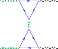
(a)

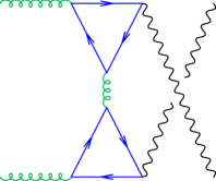
(b)

Figure 6: Two-loop anomaly style diagrams for the production of $Z$ boson pairs.

The two-loop $gg\to ZZ$ amplitude contains, in addition, two topologies which consist of products of one-loop sub-diagrams. On the one hand diagrams containing gluon self-energy contributions vanish due to color conservation. The diagrams in Fig. 6, on the other hand, give a finite mass dependent contribution as long as both $Z$ bosons couple to distinct fermion loops. These diagrams are proportional only to the axial coupling of the $Z$ bosons to fermions; the vector component vanishes due to $C$ invariance (Furry’s theorem). The diagrams have been omitted in the previous section since they can be computed with their full top mass dependence and, therefore, need no large-mass expansion Kniehl:1989qu ; Campbell:2007ev .

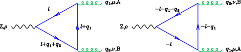
Figure 7: Triangle diagrams representing the $Zgg$ form factor at lowest order.

In brevity we repeat the results from Campbell:2007ev and give the result in terms of our conventions. Let us denote the amplitude for a $Z$ coupling to two gluons by $T^{\mu\nu\rho}_{AB}$. We calculate the triangle shown in Fig. 7, where all momenta are outgoing $q_{1}+q_{2}+q_{3}=0$ and to begin with $q_{1}^{2}\neq 0,q_{2}^{2}\neq 0$. The result for the two triangle diagrams (including the minus sign for a fermion loop) is,

$$T^{\mu\nu\rho}_{AB}(q_{1},q_{2})=i\frac{g_{s}^{2}}{16\pi^{2}}\frac{1}{2}\delta_{AB}\Big{(}\frac{g_{W}}{2\cos\theta_{W}}\Big{)}\tau_{f}\;\Gamma^{\mu\nu\rho}\,,$$ (48)

where $\tau_{f}=\pm 1/2$ and,

$$\Gamma^{\mu\nu\rho}(q_{1},q_{2},m)=\frac{2}{i\pi^{2}}\int\;d^{d}l\;\mbox{Tr}\Big{\{}\gamma^{\rho}\gamma_{5}\frac{1}{\hbox to0.0pt{$\;\!\!\not$\hss}{l}-m}\gamma^{\mu}\frac{1}{\hbox to0.0pt{$\;\!\!\not$\hss}{l}+\hbox to0.0pt{$\;\!\!\not$\hss}{q}_{1}-m}\gamma^{\nu}\frac{1}{\hbox to0.0pt{$\;\!\!\not$\hss}{l}+\hbox to0.0pt{$\;\!\!\not$\hss}{q}_{1}+\hbox to0.0pt{$\;\!\!\not$\hss}{q}_{2}-m}\Big{\}}\,.$$ (49)

The most general form of $\Gamma$ consistent with QCD gauge invariance,

$$q_{1}^{\mu}\Gamma_{\mu\nu\rho}=q_{2}^{\nu}\Gamma_{\mu\nu\rho}=0\;,$$ (50)

can be written as,

$$\Gamma^{\mu\nu\rho} = F_{1}(q_{1},q_{2},m)\;\Big{\{}\mbox{Tr}[\gamma^{\rho}\gamma^{\nu}\hbox to0.0pt{$\;\!\!\not$\hss}{q_{1}}\hbox to0.0pt{$\;\!\!\not$\hss}{q_{2}}\gamma_{5}]q_{1}^{\mu}+\mbox{Tr}[\gamma^{\rho}\gamma^{\mu}\gamma^{\nu}\hbox to0.0pt{$\;\!\!\not$\hss}{q_{2}}\gamma_{5}]q_{1}^{2}\Big{\}}$$ (51)

$$+ F_{2}(q_{1},q_{2},m)\;\Big{\{}\mbox{Tr}[\gamma^{\rho}\gamma^{\mu}\hbox to0.0pt{$\;\!\!\not$\hss}{q_{1}}\hbox to0.0pt{$\;\!\!\not$\hss}{q_{2}}\gamma_{5}]q_{2}^{\nu}+\mbox{Tr}[\gamma^{\rho}\gamma^{\mu}\gamma^{\nu}\hbox to0.0pt{$\;\!\!\not$\hss}{q_{1}}\gamma_{5}]q_{2}^{2}\Big{\}}$$

$$+ F_{3}(q_{1},q_{2},m)\;(q_{1}^{\rho}+q_{2}^{\rho})\Big{\{}\mbox{Tr}[\gamma^{\mu}\gamma^{\nu}\hbox to0.0pt{$\;\!\!\not$\hss}{q_{1}}\hbox to0.0pt{$\;\!\!\not$\hss}{q_{2}}\gamma_{5}]\Big{\}}$$

$$+ F_{4}(q_{1},q_{2},m)\;(q_{1}^{\rho}-q_{2}^{\rho})\Big{\{}\mbox{Tr}[\gamma^{\mu}\gamma^{\nu}\hbox to0.0pt{$\;\!\!\not$\hss}{q_{1}}\hbox to0.0pt{$\;\!\!\not$\hss}{q_{2}}\gamma_{5}]\Big{\}}\,.$$

By direct calculation it is found that $F_{4}=0$.

Contracting with the momentum of the $Z$ boson we find that, $q_{3}=-q_{1}-q_{2}$

$$(q_{3})_{\rho}\,\Gamma^{\mu\nu\rho}=\Big{[}-q_{1}^{2}\,F_{1}(q_{1},q_{2},m)+q_{2}^{2}\,F_{2}(q_{1},q_{2},m)-q_{3}^{2}\,F_{3}(q_{1},q_{2},m)\Big{]}\mbox{Tr}[\gamma^{\mu}\gamma^{\nu}\hbox to0.0pt{$\;\!\!\not$\hss}{q_{1}}\hbox to0.0pt{$\;\!\!\not$\hss}{q_{2}}\gamma_{5}]\,.$$ (52)

The divergence of the axial current is found by direct calculation to be,

$$(q_{3})_{\rho}\,\Gamma^{\mu\nu\rho}=\Big{[}4m^{2}C_{0}(q_{1},q_{2};m,m,m)+2\Big{]}\mbox{Tr}[\gamma^{\mu}\gamma^{\nu}\hbox to0.0pt{$\;\!\!\not$\hss}{q_{1}}\hbox to0.0pt{$\;\!\!\not$\hss}{q_{2}}\gamma_{5}]$$ (53)

showing the contribution of the pseudoscalar current proportional to $m^{2}$ and the anomalous piece. Summation over one complete quark doublet ($\tau_{f}=\pm 1/2$) cancels the anomaly term and solely the piece proportional to the top mass remains.

For the particular case at hand we are interested in on-shell $Z$’s and in $q_{2}^{2}=\varepsilon_{2}\cdot q_{2}=0,\,\varepsilon_{3}\cdot q_{3}=0,\,q_{3}=-q_{1}-q_{2}$, so we get a contribution only from $F_{1}$. The result for $F_{1}$ is

$$F_{1}(q_{1},q_{2},m) = \frac{1}{2q_{1}\cdot q_{2}}\Bigg{[}2+4m^{2}C_{0}(q_{1},q_{2};m,m,m)$$ (54)

$$+ \Big{(}2+\frac{q_{1}^{2}}{q_{1}\cdot q_{2}}\Big{)}\Big{[}B_{0}(q_{1}+q_{2};m,m)-B_{0}(q_{1};m,m)\Big{]}\Bigg{]}\,,$$

$$F_{1}(q_{1},q_{2},0) = \frac{2}{(q_{3}^{2}-q_{1}^{2})}\Bigg{[}1+\frac{q_{3}^{2}}{(q_{3}^{2}-q_{1}^{2})}\log(\frac{q_{1}^{2}}{q_{3}^{2}})\Bigg{]}\,.$$ (55)

We further define a subtracted $F_{1}$ to take into account the contribution of the top and the bottom quarks,

$${{\cal F}_{1}}(q_{1},q_{2},m)=\Big{[}F_{1}(q_{1},q_{2},m)-F_{1}(q_{1},q_{2},0)\Big{]}\,.$$ (56)

Analogous to Eq. (38) we define the projected matrix element for the anomaly piece

$$\ket{{\cal B}^{0}_{\text{anom}}(\alpha_{S}^{0},m^{0},\mu,\epsilon)}=\frac{\delta^{AB}}{N_{A}}\left(g^{\mu\nu}\,p_{1}p_{2}-p_{2}^{\mu}p_{1}^{\nu}\right)P_{Z}^{\alpha\rho^{\prime}}(p_{3})P_{Z,\rho^{\prime}}^{\beta}(p_{4})\ket{{\cal B}_{\text{anom},\mu\nu\alpha\beta}^{0,AB}(\alpha_{S}^{0},m^{0},\mu,\epsilon)}\,.$$ (57)

The amplitude defined in Eq. (57) is UV and IR finite and requires no renormalisation. Including the effect of both the $b$ quark (taken to be massless) and the $t$ quark we obtain (No statistical factor for identical $Z$ bosons is included).

$$\ket{{\cal B}_{\text{anom}}(\alpha_{S}^{(n_{l})},m,\mu)} =a_{t}^{2}s^{2}\mathcal{N}\cdot\left(\frac{\alpha_{S}^{(n_{l})}}{4\pi}\right)^{2}$$ (58)

$$\times\Bigg{\{}\Big{[}(r_{Z}-x)\big{(}1+(r_{Z}-x)(1/r_{Z}-1/(2r_{Z}^{2}))\big{)}\Big{]}{\cal F}_{1}(p_{1}-p_{3},-p_{1},m){\cal F}_{1}(p_{3}-p_{1},-p_{2},m)$$

$$+\Big{[}(r_{Z}-1+x)\big{(}1+(r_{Z}-1+x)(1/r_{Z}-1/(2r_{Z}^{2}))\big{)}\Big{]}{\cal F}_{1}(p_{1}-p_{4},-p_{1},m){\cal F}_{1}(p_{4}-p_{1},-p_{2},m))\Bigg{\}}\,,$$

where ${\cal N}$ is given in Eq. (18). Again we include the factors $s^{2}$ to indicate the correct dimensionality of ${\cal F}_{1}(p_{1},p_{2},m)$. For completeness we also give the mass expansion of Eq. (58) in case only the top quark contribution is considered, i.e. $F_{1}(p_{1},p_{2},0)\to 0$. As expected the expansion starts at $1/m^{4}$.

$$\ket{{\cal B}_{\text{anom,t}}(\alpha_{S}^{(n_{l})},m,\mu)} =a_{t}^{2}\mathcal{N}\cdot\left(\frac{\alpha_{S}^{(n_{l})}}{4\pi}\right)^{2}\;\Bigg{\{}\frac{1}{r_{t}^{2}}\left[-\frac{1}{9}+\frac{r_{Z}}{9}+\frac{1-\tilde{x}}{18r_{Z}}+\frac{-1+2\tilde{x}}{72r_{Z}^{2}}\right]+\frac{1}{r_{t}^{3}}\left[-\frac{8r_{Z}}{135}+\frac{2r_{Z}^{2}}{45}\right.$$

$$+\left.\frac{(13-18\tilde{x})}{270}+\frac{1-3\tilde{x}}{270r_{Z}^{2}}+\frac{-11+26\tilde{x}}{540r_{Z}}\right]+\frac{1}{r_{t}^{4}}\left[-\frac{22r_{Z}^{2}}{945}+\frac{22r_{Z}^{3}}{1575}+\frac{r_{Z}(1511-2362\tilde{x})}{56700}\right.$$

$$+\left.\frac{-3845+9892\tilde{x}}{226800}-\frac{191\left(1-4\tilde{x}+2\tilde{x}^{2}\right)}{226800r_{Z}^{2}}+\frac{646-2129\tilde{x}+382\tilde{x}^{2}}{113400r_{Z}}\right]+\frac{1}{r_{t}^{5}}\left[-\frac{38r_{Z}^{3}}{4725}+\frac{19r_{Z}^{4}}{4725}\right.$$

$$+\frac{r_{Z}^{2}(113-188\tilde{x})}{9450}+\frac{r_{Z}(-783+2104\tilde{x})}{75600}+\frac{-111+472\tilde{x}-306\tilde{x}^{2}}{75600r_{Z}}+\frac{1-5\tilde{x}+5\tilde{x}^{2}}{5400r_{Z}^{2}}$$

$$+\left.\frac{197-688\tilde{x}+194\tilde{x}^{2}}{37800}\right]+\frac{1}{r_{t}^{6}}\left[-\frac{1613r_{Z}^{4}}{623700}+\frac{1613r_{Z}^{5}}{1455300}+\frac{r_{Z}^{3}(41432-71573\tilde{x})}{8731800}\right.$$ (59)

$$+\frac{r_{Z}^{2}(-457682+1261401\tilde{x})}{87318000}+\frac{-1049213+4652126\tilde{x}-3464248\tilde{x}^{2}}{698544000}$$

$$+\frac{r_{Z}\left(622783-2250826\tilde{x}+764954\tilde{x}^{2}\right)}{174636000}+\frac{42658-222727\tilde{x}+251038\tilde{x}^{2}-18874\tilde{x}^{3}}{116424000r_{Z}}$$

$$+\left.\frac{9437\left(-1+6\tilde{x}-9\tilde{x}^{2}+2\tilde{x}^{3}\right)}{232848000r_{Z}^{2}}\right]+{\cal O}\left(1/r_{t}^{7},\epsilon\right)\Bigg{\}}\,.$$

3.5 Visualisation of Large-Mass Expansion Results for $gg\to ZZ$

Let us turn towards the graphical representations of the large-mass expansion results for the SM continuum, Eqs. (3.3-3.4.1), and their improvements. We proceed analogously to Sec. 2.2.3 and compute the UV+IR renormalised version of Eq. (3.1) and again integrate over the $ZZ$ phase space. The setup from Eq. (2.2.3) is utilised. Since we focus our discussion in this section mainly on the different improvements of the large-mass expansions we, again, do not take into account the full NLO correction. We merely focus on the unknown virtual massive two-loop contribution of the SM continuum interfered with the Higgs-mediated process. That is, we set

$$\sigma_{\text{int}}^{\text{LO}}\sim 2\,{\rm Re}\bra{{\cal F}_{\cal A}^{(1)}(m,\mu)}\ket{{\cal F}_{\cal B}^{(1)}(m,\mu)}\quad\text{and}\quad\sigma_{\text{virt,int}}^{\text{NLO}}\sim 2\,{\rm Re}\bra{{\cal F}_{\cal A}^{(1)}(m,\mu)}\ket{{\cal F}_{\cal B}^{(2)}(m,\mu)}\,,$$ (60)

which also excludes the anomaly style contribution from eq (58) since this part can be computed without the necessity of any approximation.

It is important to notice the following conventions for our approximations using Padé approximants below. As in Sec. 2.2.3 the Padé approximants are computed at amplitude level for each finite remainder ${\cal F}_{{\cal A},{\cal B}}$, including the conformal mapping. We know from our previous discussion that the best approximation of the LO as well as the virtual NLO contribution of the Higgs-mediated process is given by ${\cal F}_{{\cal A},[5/5]}^{(1,2)}$. It is understood that we will always use this approximant in the following considerations. In principle, we can also substitute the approximated Higgs-mediated amplitude ${\cal F}_{{\cal A},[5/5]}^{(1)}$ with its exact LO result. Doing so would remove any uncertainties from the Higgs-mediated contribution. On the other hand the numerical difference between both approaches is negligible as discussed in Sec. 2.2.3.

The vector-vector part of the SM continuum gives only a minor contribution to the total cross section, $\sigma_{VV}/\sigma_{AA}\sim 10^{-3}$. This relies on the fact that the mass expansion of the $VV$ part starts only at $1/m^{4}$ whereas the $AA$ part starts at $1/m^{2}$ and additionally $a_{t}^{2}/v_{t}^{2}\sim 7$.

The interference including the exact top mass dependence is only known at leading-order, which is shown in the left panel of Fig. 8. Comparing the exact result (black) and its naive large-mass approximation up to $1/m^{12}$ (orange) shows excellent agreement up to $s\sim 3m^{2}$, with approximately $1\%$ deviation from the exact result. At threshold the deviation rises to $12\%$. In contrast the Padé approximant ${\cal F}_{{\cal B},[3/3]}^{(1)}$ (blue) deviates from the exact result by $6\%$ at threshold. The shaded grey area indicates the variation from computing the Padé approximants $[2/2],[2/3],[3/2],[3/3]$ with $3-8\%$ deviation at threshold. Due to the change of sign of their derivatives we get a better approximation closely above threshold, as can be seen in the bottom plot of Fig. 8. Nevertheless, the peak of the exact LO result at $s\sim 5.2m^{2}$ is with $10-11\%$ deviation quite poorly approximated. Ineptly this is the region of interest for our later analysis of the Higgs boson width. Going to large values of $s$ the deviations inevitably become larger, but the contribution to the cross section is small due to the suppression by the flux.

This situation seems to continue in case of the next-to-leading-order large-mass expansion as shown in the right panel of Fig. 8. Evidently no exact result is available and we have to rely on the approximate results. All Padé approximants $[2/2],[2/3],[3/2],[3/3]$ for ${\cal F}_{\cal B}^{(2)}$ show a stable trend over the entire $s/m^{2}$ range. The deviations between the diagonal and non-diagonal Padé approximants are again indicated by the shaded grey area and the approximant ${\cal F}_{{\cal B},[3/3]}^{(2)}$ is shown in orange. The steeper rise near the top threshold suggests a better description of the actual threshold properties of the NLO result with exact top mass dependence in contrast to the naive large-mass expansion (black). Comparing the trend above threshold with its analogous LO situation we can only guess that we have to expect comparable deviations from our Padé approximations with respect to the unknown exact NLO result.

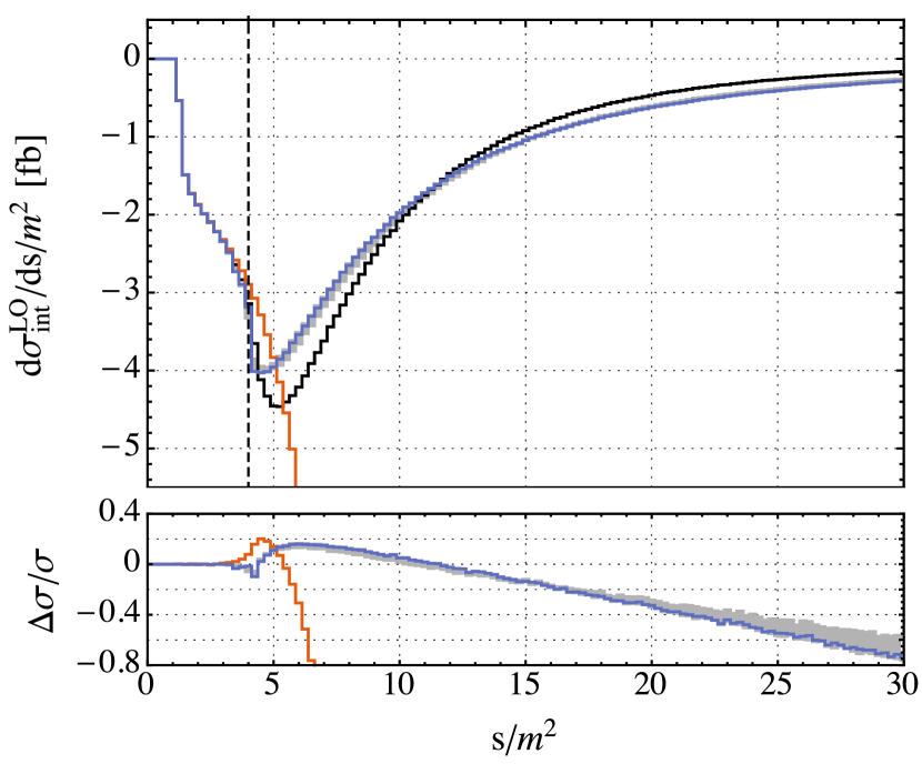
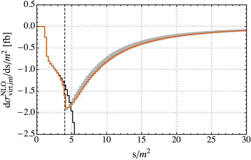
Figure 8: Left panel: Leading-order interference ${\rm Re}\bra{{\cal F}_{\cal A}^{(1)}(m,\mu)}\ket{{\cal F}_{\cal B}^{(1)}(m,\mu)}$. Exact result (black), LME up to $1/m^{12}$ (orange) and envelope of Padé approximants $[2/2],[2/3],[3/2]$ and $[3/3]$ (blue) as grey area. Bottom plot shows the relative deviation from the exact result. Right panel: Next-to-leading-order interference ${\rm Re}\bra{{\cal F}_{\cal A}^{(1)}(m,\mu)}\ket{{\cal F}_{\cal B}^{(2)}(m,\mu)}$. LME up to $1/m^{12}$ (black) and envelope of Padé approximants $[2/2],[2/3],[3/2]$ and $[3/3]$ (orange) as grey area. The vertical dashed line denotes the top quark pair-production threshold. See text for details.

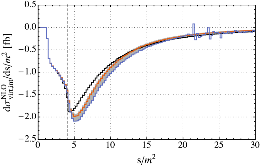
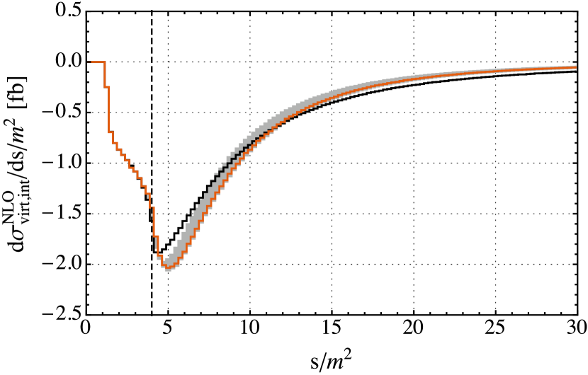
Figure 9: Next-to-leading-order interference ${\rm Re}\bra{{\cal F}_{\cal A}^{(1)}(m,\mu)}\ket{{\cal F}_{\cal B}^{(2)}(m,\mu)}$. Left panel: Interference by rescaling, Eq. (26). Padé approximant $[3/3]$ as comparison (black). Envelope of $\sigma_{\text{imp},n}^{\text{NLO}}$ for $n=\{1,\ldots,6\}$ as grey area; $n=1$ (orange) and $n=6$ (blue) shown explicitly. Right panel: Interference by alternative rescaling, Eq. (61). Padé approximant $[3/3]$ as comparison (black). Grey area given by envelope of $\sigma_{\text{imp},[n/m]}^{\text{NLO}}$ with $n,m=\{2,3\}$; $[3/3]$ shown explicitly (orange). The vertical dashed line denotes the top quark pair-production threshold. See text for details.

We can also consider rescaling the NLO large-mass expansion as described in Eq. (26). The resulting curves are shown in the left panel of Fig. 9. To guide the eye we also include ${\cal F}_{{\cal B},[3/3]}^{(2)}$ (black). The envelope of the different orders $n$ in the expansion $\sigma_{\text{imp},n}^{\text{NLO}}$ is shown as grey area. For $s\leq 20m^{2}$ the envelope is determined from $n=\{1,\ldots,6\}$, whereas for $s>20m^{2}$ we only use $n=\{1,\ldots,5\}$ due to the instabilities for $n=6$ in the high energy regime. The most interesting curves, namely the heavy-quark approximation $n=1$ and the highest order in the expansion $n=6$, are shown in orange and blue, respectively. Factoring out the exact LO result seems to give a more natural description of the threshold behaviour and peak structure in comparison to the plain use of the Padé approximation.

The origin of the numerical instabilities of the $n=6$ expansion is probably due to delicate numerical cancellations in the $(s/m^{2})^{6}$ coefficients. One could try to cure this problem by switching to a higher numerical precision or by a proper economisation Press:2007:NRE:1403886 of the power series. With the Padé approximation we already have an excellent method at hand and we adopt the idea of factoring out the exact LO interference,

$$\sigma_{\text{imp},[n/m]}^{\text{NLO}}=\sigma_{\text{exact}}^{\text{LO}}\cdot\frac{\sigma_{[n/m]}^{\text{NLO}}}{\sigma_{[n/m]}^{\text{LO}}}\,.$$ (61)

Keeping our usual definition in mind $\sigma_{\text{imp},[n/m]}^{\text{(N)LO}}$ denotes the (virtual N)LO contribution using ${\cal F}_{{\cal A},[5/5]}^{(1)}$ and ${\cal F}_{{\cal B},[n/m]}^{(1,2)}$. The result is shown in Fig. 9, right panel. We immediately see the advantages of this approach. Firstly we also get a similar, more natural behaviour at threshold and of the peak structure above threshold. Secondly we get a stable result across the entire range of $s/m^{2}$. The grey area is again given by the envelopes due to the variation between the (non-)diagonal Padé approximants $[2/2],[2/3],[3/2]$ and $[3/3]$(orange). Ultimately by using the Padé approximants in contrast to Eq. (26) we could entirely remove the uncertainty of having to use an approximation for the involved Higgs-mediated amplitude and fall back to using the exactly known result for ${\cal F}_{{\cal A}}^{(1)}$.

Some concluding remarks. In contrast to the purely Higgs-mediated case, Sec. 2.2.3, it turns out that we require the Padé approximation in the interference case. Using the conformal mapping alone without an additional Padé approximant on top gives no reasonable approximation for the quantities discussed above. On the other hand we have seen that we hugely benefit by using Padé approximations due to their stability and the possibility of removing any uncertainty besides the approximated virtual massive two-loop $gg\to ZZ$ amplitude.

4 Real Corrections to SM $ZZ$ Production

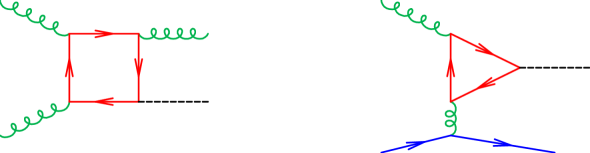
Figure 10: Representative diagrams for the $0\to ggHg$ and the $0\to gHq\bar{q}$ amplitudes.

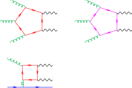
Figure 11: Representative diagrams for the $0\to ggZZg$ and the $0\to gZZq\bar{q}$ amplitudes.

Representative diagrams for the real radiation contributions to this process are shown in Figs. 10 and 11. The Higgs-mediated diagrams have previously been computed in Ellis:1987xu . They can easily be adapted to our calculation by combining those results with the decay amplitude given in Eq. (16) and ${\cal N}$ from Eq. (18). This procedure, together with the strategy for handling the amplitudes for diagrams without a Higgs boson, is described in detail in Campbell:2014gua . We adopt this implementation here. Our calculation of the pure-Higgs contribution involves the computation of the square of the diagrams shown in Fig. 10, together with all crossings of the quarks in Fig. 10 (right) into the initial state. Similarly, the interference contribution includes all crossings of the diagrams shown in Fig. 11. In principle another contribution to the interference occurs at this order, between tree-level amplitudes for the process $qg\to ZZq$ and the $qg$-initiated diagrams shown in Fig. 10 (right) and 11 (bottom-left). However this contribution is subleading Campbell:2014gua , particularly for high invariant masses of the $ZZ$ system, so we do not consider it here.

The real radiation diagrams contain infrared singularities, of soft and collinear origin, that must be isolated and combined with the corresponding poles in the two-loop amplitudes. This is handled using the dipole subtraction procedure Catani:1996vz .

5 Results

The individual components of the calculation that have been extensively discussed above have been included in the parton-level Monte Carlo code MCFM Campbell:1999ah ; Campbell:2011bn ; Campbell:2015qma . The bulk of the calculation is performed in a straightforward manner using the normal operation of MCFM at NLO. The exception is the finite contribution to the two-loop amplitude containing a closed loop of massless quarks. Since these contributions are computationally expensive to evaluate, we choose to include their effects by reweighting an unweighted sample of LO events.

For the two-loop amplitudes containing massive loops of quarks the approximations used are as follows. The Higgs amplitude is evaluated using the $[5/5]$ Padé approximant to the LME after conformal mapping. As demonstrated in Sec. 2, this is virtually identical to the exact result. The massive quark box contributions are computed by factoring out the exact LO amplitude according to Eq. (61), with the Padé approximant corresponding to $n=m=3$ in the definition given in Eq. (28). The anomalous diagrams of Sec. 3.4.2 are not included in the discussion of the massive quark loops below, but instead are accounted for only when the sum of all loops is considered.

For massless quarks circulating in the loop the calculation is simplified by the fact that the entire amplitude is proportional to the combination of couplings $(v_{f}^{2}+a_{f}^{2})$, i.e. in the decomposition given in Eq. (40) the quantities $\ket{\widetilde{{\cal B}}_{VV}^{0}}$ and $\ket{\widetilde{{\cal B}}_{AA}^{0}}$ are equal. The calculation requires the one-loop master integrals up to $\epsilon^{2}$, for which all orders results are given in ref. Smirnov:2006ry for bubble integrals and refs. Bern:1994zx ; Bern:1993kr ; Brandhuber:2004yw ; Brandhuber:2005kd ; Cachazo:2004zb for the easy box (two opposite off-shell legs). The necessary results for the three-mass triangle with massless propagators and the hard box (two adjacent off-shell legs) can be taken from refs. Chavez:2012kn and Anastasiou:2014nha respectively. We use the coproduct formalism Duhr:2012fh ; Duhr:2014woa to analytical continue the results to the physical phase space regions. All master integrals have been numerically cross-checked with SecDec Borowka:2015mxa . The two-loop master integrals for $gg\to ZZ$ are taken from ref. Gehrmann:2014bfa and GiNaC is used to evaluate the polylogarithms. Our results for this contribution agree with the earlier calculation of ref. vonManteuffel:2015msa .

The parameters for the following results have already been specified in Sec. 2.2.3. Here we make only one change: our central scale corresponds to the choice $\mu_{r}=\mu_{f}=M_{ZZ}/2$, where $M_{ZZ}$ is the invariant mass of the $ZZ$ pair. As an estimate of the theoretical uncertainty we consider variations by a factor of two about this value. We also introduce an uncertainty that is based on our combination of LME and Padé approximants in the calculation of the massive quark loops, that has already been explored in Fig. 9 (right). In order to obtain a more conservative error estimate we multiply the deviations of the extremal values in the grey area with respect to $\sigma_{\text{imp},[3/3]}^{\text{NLO}}$ by a factor of two. The impact of this variation on the complete NLO prediction for the massive loop is shown in Fig. 12. Even for this choice, the impact of the approximation is estimated to be less than $20$% throughout the distribution. For the remaining plots in this section we no longer show the impact of this uncertainty, but it will be explicitly included in Tables 2 and 3 later on.

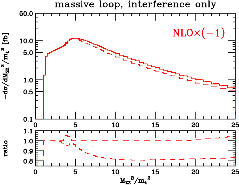
Figure 12: The uncertainty on the calculation of the massive loop interference contribution stemming from the use of the LME expansion and Padé approximants. The central result is shown as a solid histogram, with the dashed lines indicating deviations that correspond to the grey area in Fig. 9, multiplied by a factor of two. All curves are computed for the central scale choice, $\mu_{r}=\mu_{f}=M_{ZZ}/2$.

Results for both the massless and massive quark contributions to the interference, including the effects of scale variation, are shown in Fig. 13. The interference is negative for both the massless and massive quark contributions and is shown in Fig. 13 reversed in sign. In both cases the $K$-factor decreases as the invariant mass of the $Z$-boson pair increases. The $K$-factor at small invariant masses is larger for the massless loops; as the invariant mass increases, the NLO corrections are more important for the massive loop. The NLO corrections are larger for the top quark loops and exhibit a stronger dependence on $M_{ZZ}$. In both cases the NLO result lies outside the estimated LO uncertainty bands and the scale uncertainty is not significantly reduced at NLO.

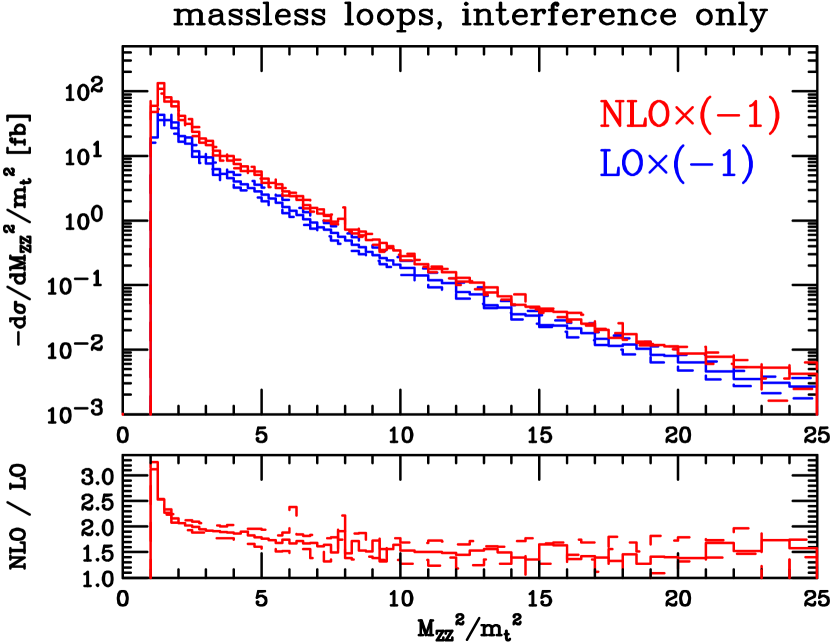
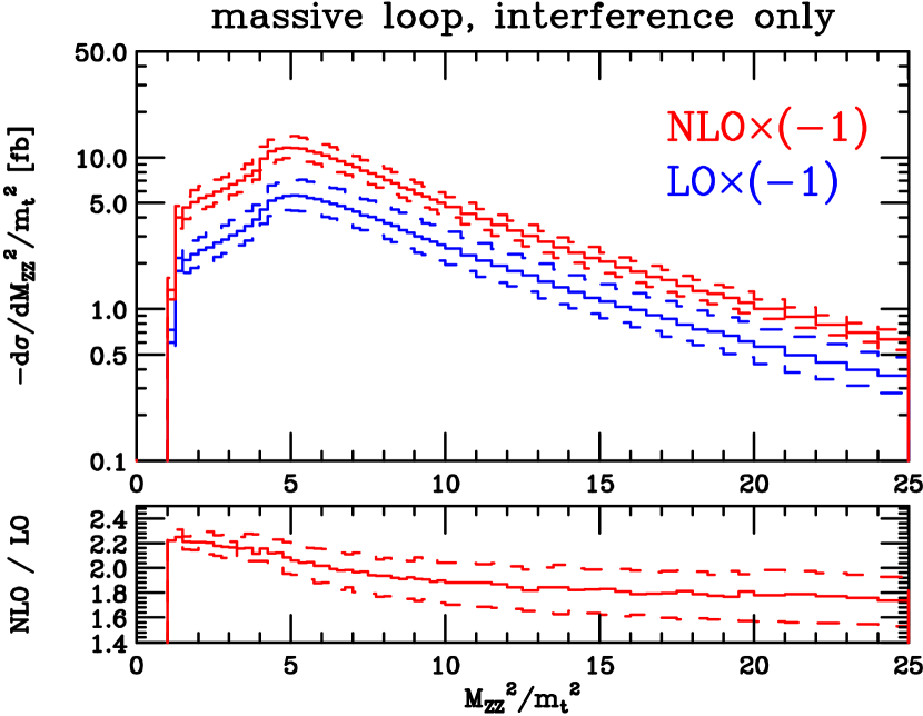
Figure 13: Left panel: Interference of the Higgs amplitude and massless quark loops at LO and NLO, with the scale uncertainty indicated by the dashed histograms. The ratio of the NLO and LO results is shown in the lower panel. Right panel: The equivalent results for the interference of the Higgs amplitude and the top quark loops.

The relative importance of the massive and massless loops can be better-assessed from the NLO predictions shown in Fig. 14. At smaller invariant masses, below the top-pair threshold, the massless loops are most important. Around the top-pair threshold the two are of a similar size, but at high energies the massless loops are insignificant. In contrast, the top quark loop quickly becomes the dominant contribution beyond this threshold and exhibits a long tail out to invariant masses of around one TeV.

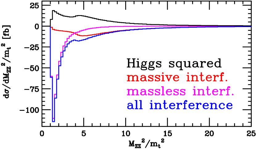
Figure 14: Comparison of the effect of the massless (magenta) and massive (red) loops in the NLO interference. Also shown is the sum (blue) and the corresponding result for the Higgs amplitude squared (black). All curves are computed for the central scale choice, $\mu_{r}=\mu_{f}=M_{ZZ}/2$.

The full prediction for the interference that is obtained by summing over both massless and top quark loops, as well as the numerically-small anomalous contribution discussed in Sec. 3.4.2, is shown in Fig. 15. The relative size of the massless and top quark loops discussed above means that the behaviour of the $K$-factor for the sum of both contributions interpolates between the massless-loop $K$-factor for small $M_{ZZ}$ and the massive loop one for high $M_{ZZ}$. It therefore decreases from around $3$ at the peak of the distribution to approximately $1.8$ in the tail. This is to be contrasted with the $K$-factor distribution for the pure Higgs amplitudes alone, shown in the right panel of Fig. 15. In that case the $K$-factor decreases slowly from around $2.2$ at small invariant masses to around $1.8$ in the far tail. We note that the $K$-factor for the Higgs amplitudes alone, and the one for the interference with the top quark loops, is almost identical. In the high-energy limit this is guaranteed to be the case, due to the cancellation between these two processes. This behaviour is shown explicitly in Fig. 16.

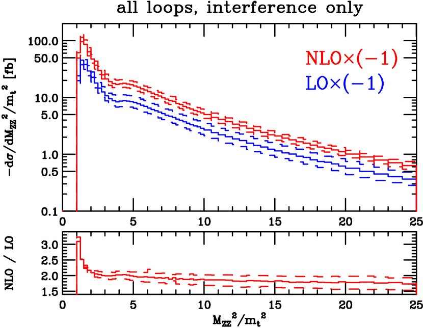
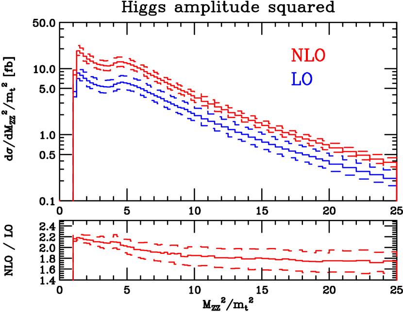
Figure 15: Left panel: Interference of the Higgs amplitude and quark loops at LO and NLO, with the scale uncertainty indicated by the dashed histograms. The ratio of the NLO and LO results is shown in the lower panel. Right panel: The equivalent results for the Higgs amplitude squared.

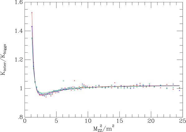
Figure 16: The ratio of the $K$-factors for the square of the Higgs diagrams alone ($K_{\mbox{higgs}}$) and the one for the interference ($K_{\mbox{inter}}$). The lines are fits to the individual histogram bins that are good to the level of a few percent and are shown for the central scale (blue) as well as the scale variations (red, green).

The integrated cross-sections for the interference contributions and the Higgs amplitude squared are shown in Table 2. Note that, in this table, the total interference differs from the sum of the massive and massless loops by a small amount that is due to the anomalous contribution. At this level the differences between the effects of the NLO corrections on the various contributions is quite small, with all corresponding to a NLO enhancement by close to a factor of two. The $K$-factor for the massless loops is slightly larger, which is also reflected in the result for the total interference. In addition to the scale uncertainty, we have also indicated our estimate of the residual uncertainty related to the LME expansion that is indicated in Fig. 12. The impact of this uncertainty is relatively small, at the level of around $5$%, due to the fact that the integrated cross-section is dominated by the region $M_{ZZ}^{2}\lesssim 5m^{2}$ where the LME is expected to work well.

Contribution	$\sigma_{LO}$ [fb]	$\sigma_{NLO}$ [fb]	$\sigma_{NLO}/\sigma_{LO}$
Higgs mediated diagrams	$56.3^{+15.3}_{-11.4}$	$111.0^{+20.1}_{-16.6}$	1.97
interference (total)	$-113.5^{+22.2}_{-29.5}$	$-237.8^{+36.4}_{-45.4}$(scale)${}^{+5.4}_{-0.4}$(LME)	2.09
interference (massless loops)	$-60.2^{+11.0}_{-14.2}$	$-132.7^{+20.5}_{-26.3}$	2.20
interference (massive loop)	$-53.3^{+11.2}_{-15.3}$	$-104.2^{+15.8}_{-18.7}$(scale)${}^{+5.4}_{-0.4}$(LME)	1.95

Table 2: Integrated cross-sections at $\sqrt{S}=13$ TeV, using the input parameters of Sec. 2.2.3 and $\mu=M_{ZZ}/2$. Uncertainties correspond to scale variation as described in the text and, for NLO results that include massive quarks, an estimate of the limitations of the LME. The $K$-factor is computed using only the central result.

For obtaining a bound on the width of the Higgs boson it is useful to focus on a high-mass region where backgrounds from the continuum processes, represented at tree-level by $q\bar{q}\to ZZ$, are small but the effect of the interference is still significant Caola:2013yja ; Campbell:2013una . To that end, in Table 3 we show the cross-sections after the application of the cut $M_{ZZ}>300$ GeV. We see that, as expected, the impact of the massive top loop on the interference is much greater, compared to the massless loops. This also has the effect of ensuring that the $K$-factors for the Higgs amplitude squared and the total interference are almost equal. To estimate the cross-section after the decays of the $Z$-bosons into electrons and muons we can simply take these results and multiply by a factor of $4\times BR(Z\to e^{-}e^{+})^{2}$, where $BR(Z\to e^{-}e^{+})=3.363\times 10^{-2}$. Assuming that the on-shell Higgs cross-section takes its Standard Model value and that the Higgs boson couplings and width are related accordingly, we can write the predictions for the off-shell region as,

$$\sigma_{4\ell}^{LO}(m_{4\ell}>300~{}\mbox{GeV})=\left(0.190^{+0.055}_{-0.040}\right)\times\left(\frac{\Gamma_{H}}{\Gamma_{H}^{SM}}\right)-\left(0.275^{+0.079}_{-0.058}\right)\times\sqrt{\frac{\Gamma_{H}}{\Gamma_{H}^{SM}}}\;\mbox{fb}\,,$$ (62)

$$\sigma_{4\ell}^{NLO}(m_{4\ell}>300~{}\mbox{GeV})=\left(0.365^{+0.064}_{-0.054}\right)\times\left(\frac{\Gamma_{H}}{\Gamma_{H}^{SM}}\right)-\left(0.526^{+0.092}_{-0.103}\right)\times\sqrt{\frac{\Gamma_{H}}{\Gamma_{H}^{SM}}}\;\mbox{fb}\,.$$ (63)

The linear terms derive from the Higgs cross-sections in Table 3 while the terms that scale as the square-root of the modified width reflect the total interference contributions. The uncertainties reflect those shown in Table 3, with the scale and LME uncertainties added linearly. It is interesting to compare these results with the corresponding on-shell Higgs cross-sections. These are given by,

$$\sigma_{4\ell}^{LO}(m_{4\ell}<130~{}\mbox{GeV})=1.654^{+0.249}_{-0.220}\;\mbox{fb}\;,\qquad\sigma_{4\ell}^{NLO}(m_{4\ell}<130~{}\mbox{GeV})=3.898^{+0.770}_{-0.560}\;\mbox{fb}\,,$$ (64)

where the uncertainties correspond to our usual scale variation procedure. From the results in Eqs. (62) and (63) it is clear that the absolute rate of off-shell events varies considerably between LO and NLO. On the other hand, the cross-sections in Eq. (64) imply that the ratio of the number of events in the off-shell region compared to the peak region is much better predicted,

$$\frac{\sigma_{4\ell}^{LO}(m_{4\ell}>300~{}\mbox{GeV})}{\sigma_{4\ell}^{LO}(m_{4\ell}<130~{}\mbox{GeV})}=\left(0.115^{+0.014}_{-0.010}\right)\times\left(\frac{\Gamma_{H}}{\Gamma_{H}^{SM}}\right)-\left(0.166^{+0.020}_{-0.015}\right)\times\sqrt{\frac{\Gamma_{H}}{\Gamma_{H}^{SM}}}\,,$$

$$\frac{\sigma_{4\ell}^{NLO}(m_{4\ell}>300~{}\mbox{GeV})}{\sigma_{4\ell}^{NLO}(m_{4\ell}<130~{}\mbox{GeV})}=\left(0.094^{+0.000}_{-0.002}\right)\times\left(\frac{\Gamma_{H}}{\Gamma_{H}^{SM}}\right)-\left(0.135^{+0.000}_{-0.008}\right)\times\sqrt{\frac{\Gamma_{H}}{\Gamma_{H}^{SM}}}\,.$$ (65)

The uncertainties in this equation are obtained by using both the LME uncertainty estimate and the scale variation, but ensuring that the cross-sections that appear in the numerator and denominator are evaluated at the same scale.

Contribution	$\sigma_{LO}$ [fb]	$\sigma_{NLO}$ [fb]	$\sigma_{NLO}/\sigma_{LO}$
Higgs mediated diagrams	$42.1^{+12.1}_{-8.8}$	$80.7^{+14.2}_{-12.0}$	1.92
interference (total)	$-60.7^{+12.8}_{-17.4}$	$-116.3^{+17.5}_{-19.9}$(scale)${}^{+5.4}_{-0.4}$(LME)	1.91
interference (massless loops)	$-12.5^{+2.5}_{-3.4}$	$-22.5^{+3.2}_{-3.2}$	1.80
interference (massive loop)	$-48.2^{+10.3}_{-14.1}$	$-93.0^{+14.0}_{-16.4}$(scale)${}^{+5.4}_{-0.4}$(LME)	1.93

Table 3: Cross-sections at $\sqrt{S}=13$ TeV in the region defined by $M_{ZZ}>300$ GeV, using the input parameters of Sec. 2.2.3. Uncertainties correspond to scale variation as described in the text and, for NLO results that include massive quarks, an estimate of the limitations of the LME. The $K$-factor is computed using only the central result.

6 Conclusions

In this paper we have presented a calculation of on-shell $Z$-boson pair production via gluon fusion at the two-loop level. This occurs both through diagrams that are mediated by a Higgs boson, with $H\to ZZ$, and by continuum contributions in which the $Z$ bosons couple through loops of quarks. We have considered contributions up to the two-loop level, corresponding to NLO corrections, for the Higgs diagrams alone and also for the interference between the two sets of diagrams.

In the continuum contribution the two-loop corrections containing loops of massless quarks are known and we have reproduced results from the literature. Our treatment of the massive quark loops is based on a large-mass expansion up to order $1/m^{12}$, that is extended to the high-mass region by using a combination of conformal mapping and Padé approximation. This procedure was shown to provide an excellent approximation of the Higgs contribution alone, where the exact result is known. Additionally, applying the large-mass expansion in combination with the conformal mapping and the Padé approximation to the $gg\to ZZ$ amplitudes is obviously not limited to the interference calculation alone. The same procedure can also be applied to the virtual two-loop $gg\to ZZ$ amplitude including its full tensor structure. It might be desirable to apply the presented procedure also to the Higgs-boson pair-production process, because the latter offers identical kinematics. Comparing those results with the recently published results including the full top mass effects Borowka:2016ehy could lead to interesting insights concerning the error estimate of the used approximation. However, this is kept as future work.

We have used our calculation to provide theoretical predictions for the impact of the interference contribution on the invariant mass distribution of $Z$-boson pairs at the $13$ TeV LHC. In the high-mass region we have shown that the impact of the NLO corrections to the interference are practically identical to those for Higgs production alone. This explicit calculation justifies using a procedure for estimating the number of off-shell events due to the interference by rescaling the LO prediction by the on-shell $K$-factor.

Appendix A Definition of Scalar Integrals

We work in the Bjorken-Drell metric so that $l^{2}=l_{0}^{2}-l_{1}^{2}-l_{2}^{2}-l_{3}^{2}$. The definition of the integrals is as follows

$$A_{0}(m)=\frac{\mu^{4-d}}{i\pi^{\frac{d}{2}}r_{\Gamma}}\int d^{d}l\;\frac{1}{(l^{2}-m^{2}+i\varepsilon)}\,,$$ (66)

$$B_{0}(p_{1};m,m)=\frac{\mu^{4-d}}{i\pi^{\frac{d}{2}}r_{\Gamma}}\int d^{d}l\;\frac{1}{(l^{2}-m^{2}+i\varepsilon)((l+p_{1})^{2}-m^{2}+i\varepsilon)}\,,$$ (67)

$$C_{0}(p_{1},p_{2};m,m,m)=\frac{\mu^{4-d}}{i\pi^{\frac{d}{2}}r_{\Gamma}}$$ (68)

$$\times\int d^{d}l\;\frac{1}{(l^{2}-m^{2}+i\varepsilon)((l+p_{1})^{2}-m^{2}+i\varepsilon)((l+p_{1}+p_{2})^{2}-m^{2}+i\varepsilon)}\,,$$

$$D_{0}(p_{1},p_{2},p_{3};m,m,m,m)=\frac{\mu^{4-d}}{i\pi^{\frac{d}{2}}r_{\Gamma}}$$ (69)

$$\times\int d^{d}l\;\frac{1}{(l^{2}-m^{2}+i\varepsilon)((l+p_{1})^{2}-m^{2}+i\varepsilon)((l+p_{1}+p_{2})^{2}-m^{2}+i\varepsilon)((l+p_{1}+p_{2}+p_{3})^{2}-m^{2}+i\varepsilon)}\,,$$

We have removed the overall constant which occurs in $d$-dimensional integrals, ($d=4-2\epsilon$)

$$r_{\Gamma}\equiv\Gamma(1+\epsilon)=1-\epsilon\gamma+\epsilon^{2}\Big{[}\frac{\gamma^{2}}{2}+\frac{\pi^{2}}{12}\Big{]}$$ (70)

with the Euler-Mascheroni constant $\gamma=0.57721\ldots$. The large mass expansion of some of these integrals are

$$B_{0}\left((p_{1}+p_{2})^{2},m,m\right) \overset{s=1}{=}\left(\frac{\mu^{2}}{m^{2}}\right)^{\epsilon}\Bigg{\{}\frac{1}{\epsilon}+\frac{1}{6}\frac{1}{r_{t}}+\frac{1+\epsilon}{60}\frac{1}{r_{t}^{2}}+\frac{(1+\epsilon)(2+\epsilon)}{840}\frac{1}{r_{t}^{3}}+\frac{6+11\epsilon+6\epsilon^{2}}{15120}\frac{1}{r_{t}^{4}}$$ (71)

$$+\frac{24+50\epsilon+35\epsilon^{2}}{332640}\frac{1}{r_{t}^{5}}+\frac{120+274\epsilon+225\epsilon^{2}}{8648640}\frac{1}{r_{t}^{6}}+\frac{180+441\epsilon+406\epsilon^{2}}{64864800}\frac{1}{r_{t}^{7}}+\frac{1260+3267\epsilon+3283\epsilon^{2}}{2205403200}\frac{1}{r_{t}^{8}}$$

$$+\frac{10080+27396\epsilon+29531\epsilon^{2}}{83805321600}\frac{1}{r_{t}^{9}}+\frac{10080+28516\epsilon+32575\epsilon^{2}}{391091500800}\frac{1}{r_{t}^{10}}+{\cal O}\left(1/r_{t}^{11},\epsilon^{3}\right)\Bigg{\}}$$

and

$$C_{0}\left(p_{1},p_{2},m,m,m\right) \overset{s=1}{=}-\left(\frac{\mu^{2}}{m^{2}}\right)^{\epsilon}\Bigg{\{}\frac{1}{2}\frac{1}{r_{t}}+\frac{1+\epsilon}{24}\frac{1}{r_{t}^{2}}+\frac{(1+\epsilon)(2+\epsilon)}{360}\frac{1}{r_{t}^{3}}+\frac{6+11\epsilon+6\epsilon^{2}}{6720}\frac{1}{r_{t}^{4}}$$ (72)

$$+\frac{24+50\epsilon+35\epsilon^{2}}{151200}\frac{1}{r_{t}^{5}}+\frac{120+274\epsilon+225\epsilon^{2}}{3991680}\frac{1}{r_{t}^{6}}+\frac{180+441\epsilon+406\epsilon^{2}}{30270240}\frac{1}{r_{t}^{7}}+\frac{1260+3267\epsilon+3283\epsilon^{2}}{1037836800}\frac{1}{r_{t}^{8}}$$

$$+\frac{10080+27396\epsilon+29531\epsilon^{2}}{39697257600}\frac{1}{r_{t}^{9}}+\frac{10080+28516\epsilon+32575\epsilon^{2}}{186234048000}\frac{1}{r_{t}^{10}}+{\cal O}\left(1/r_{t}^{11},\epsilon^{3}\right)\Bigg{\}}\,.$$

for $p_{1}^{2}=p_{2}^{2}=0,(p_{1}+p_{2})^{2}=s$.

Appendix B Scale Dependence of the Finite Remainder

In this section we shortly summarise a convenient, and well-known, way to determine the dependence on the renormalisation scale $\mu=\mu_{r}$ of the one- and two-loop finite remainders used within this work, i.e. processes with a loop-induced leading-order matrix element. This determination is possible by exploiting the renormalisation group equation (RGE) properties of the individual building block, e.g. $\alpha_{S}^{(n_{f})}(\mu)$, as discussed below. Knowledge of this scale dependence, in return, offers a simple way to compute finite remainder results at arbitrary scales, provided the results at a starting scale $\mu_{0}$ are known. We mostly recycle our definitions from Sec. 2.1. In the following, however, we stick to a slightly more general notation when applicable. To this end we drop the amplitude specifications ${\cal A}$ and ${\cal B}$ from the finite remainder definition in Eq. (11) and denote our previous amplitudes ${\cal A}$ and ${\cal B}$ simply by ${\cal M}$. We also replace our, to the $gg\to ZZ$ process specialised, IR constant $\hat{\bm{Z}}_{gg}^{(n_{l})}$ from Eq. (14) by a more general IR constant $\hat{\bm{Z}}_{IR}$ following the notation in Ferroglia:2009ii ; Baernreuther:2013caa ; Czakon:2014oma . The finite remainder for $n_{f}$ quark flavours is thus defined by

$$\ket{{\cal F}(\alpha_{S}^{(n_{f})},m,\mu)} =\frac{1}{\hat{\bm{Z}}_{IR}}\,\ket{{\cal M}^{r}(\alpha_{S}^{(n_{f})},m,\mu)}=\frac{Z_{UV}^{(n_{f})}}{\hat{\bm{Z}}_{IR}}\left(\frac{N^{\epsilon}Z^{(n_{f})}_{\alpha_{S}}\alpha_{S}^{(n_{f})}(\mu)}{4\pi}\right)\Bigg{[}\ket{{\cal M}^{(1),0}(m)}$$

$$+\left(\frac{N^{\epsilon}Z^{(n_{f})}_{\alpha_{S}}\alpha_{S}^{(n_{f})}(\mu)}{4\pi}\right)\ket{{\cal M}^{(2),0}(m)}\Bigg{]}+{\cal O}\left((\alpha_{S}^{(n_{f})})^{3}\right)\,.$$ (73)

The mass dependence does not play any important role in the subsequent discussion and, hence, all results are valid for arbitrary masses $m$. $Z_{UV}^{(n_{f})}$ denotes the process dependent $UV$ renormalisation constants and the mass renormalisation $m^{0}=Z_{m}m$ is again kept implicit. The strong coupling constants $\alpha_{S}$ is renormalised according to

$$\alpha_{S}^{0}=N^{\epsilon}Z^{(n_{f})}_{\alpha_{S}}\alpha_{S}^{(n_{f})}(\mu)\quad\text{with}\quad N^{\epsilon}=\mu^{2\epsilon}\frac{e^{\epsilon\,\gamma_{E}}}{(4\pi)^{\epsilon}}\,,$$ (74)

where the explicit $\mu$ dependence from the loop measure in Eq. (4) was shifted to $N^{\epsilon}$. The renormalisation constant $Z^{(n_{f})}_{\alpha_{S}}$ and the coefficient of the beta function $\beta_{0}^{(n_{f})}$ are given in Eq. (9). The explicit scale and flavour dependence of $\alpha_{S}=\alpha_{S}^{(n_{f})}(\mu)$ is neglected in the following for simplicity.

Equivalently to Eq. (B) we define the perturbative expansion of the finite remainder as

$$\ket{{\cal F}(\alpha_{S},m,\mu)}=\frac{\alpha_{S}}{4\pi}\ket{{\cal F}^{(1)}(m,\mu)}+\left(\frac{\alpha_{S}}{4\pi}\right)^{2}\ket{{\cal F}^{(2)}(m,\mu)}+{\cal O}\left(\alpha_{S}^{3}\right)\,.$$ (75)

Taking the derivative with respect to $\mu^{2}$ of Eq. (B) and Eq. (75) leads to

$$\mu^{2}\frac{d\,}{d\mu^{2}}\ket{{\cal F}(\alpha_{S},m,\mu)} =\left(\mu^{2}\frac{d}{d\mu^{2}}\left(\frac{\alpha_{S}}{4\pi}\right)\right)\ket{{\cal F}^{(1)}(m,\mu)}+\frac{\alpha_{S}}{4\pi}\;\mu^{2}\frac{d\,}{d\mu^{2}}\ket{{\cal F}^{(1)}(m,\mu)}$$

$$+2\left(\frac{\alpha_{S}}{4\pi}\right)\left(\mu^{2}\frac{d\,}{d\mu^{2}}\left(\frac{\alpha_{S}}{4\pi}\right)\right)\ket{{\cal F}^{(2)}(m,\mu)}+\left(\frac{\alpha_{S}}{4\pi}\right)^{2}\;\mu^{2}\frac{d\,}{d\mu^{2}}\ket{{\cal F}^{(2)}(m,\mu)}$$ (76)

$$=\mu^{2}\frac{d\,}{d\mu^{2}}\Bigg{\{}\frac{Z_{UV}^{(n_{f})}}{\hat{\bm{Z}}_{IR}}\left(\frac{N^{\epsilon}Z^{(n_{f})}_{\alpha_{S}}\alpha_{S}^{(n_{f})}(\mu)}{4\pi}\right)\Bigg{[}\ket{{\cal M}^{(1),0}(m)}$$

$$+\left(\frac{N^{\epsilon}Z^{(n_{f})}_{\alpha_{S}}\alpha_{S}^{(n_{f})}(\mu)}{4\pi}\right)\ket{{\cal M}^{(2),0}(m)}\Bigg{]}\Bigg{\}}\,.$$

The derivatives of $Z_{UV}^{(n_{f})}$ and $Z_{m}$ vanish because these renormalisation constants are defined in the on-shell scheme. The explicit $\mu$ dependence within these expressions cancels against the $\alpha_{S}$ scale dependence. The derivative of $\hat{\bm{Z}}_{IR}$ with respect to $\mu$ is given by its RGE Ferroglia:2009ii ; Baernreuther:2013caa ; Czakon:2014oma and therefore

$$\mu^{2}\frac{d\,}{d\mu^{2}}\frac{1}{\hat{\bm{Z}}_{IR}}=-\frac{1}{\hat{\bm{Z}}_{IR}^{2}}\frac{1}{2}\;\underbrace{\frac{d}{d\log\mu}\hat{\bm{Z}}_{IR}}_{-\hat{\Gamma}\cdot\hat{\bm{Z}}_{IR}}=\frac{\alpha_{S}}{4\pi}\frac{\hat{\Gamma}^{(1)}}{2}\cdot\frac{1}{\hat{\bm{Z}}_{IR}}+{\cal O}\left(\alpha_{S}^{2}\right)\,.$$ (77)

The anomalous dimension operator $\hat{\Gamma}$ can be taken from Czakon:2014oma and references therein. For our $gg\to ZZ$ processes $\hat{\Gamma}$ simplifies to

$$\hat{\Gamma}=\frac{\alpha_{S}}{4\pi}\,\hat{\Gamma}^{(1)}+{\cal O}\left(\alpha_{S}^{2}\right) =\frac{\alpha_{S}}{4\pi}\left(-4C_{A}\log\left(\frac{\mu^{2}}{-s-i\epsilon}\right)-2\beta_{0}^{(n_{f})}\right)+{\cal O}\left(\alpha_{S}^{2}\right)$$ (78)

$$=\frac{\alpha_{S}}{4\pi}\left(\hat{K}^{(1)}+\hat{D}^{(1)}\cdot\log\left(\frac{\mu^{2}}{\mu_{0}^{2}}\right)\right)+{\cal O}\left(\alpha_{S}^{2}\right)$$

with

$$\hat{K}^{(1)}=-4C_{A}\,\log\left(\frac{\mu_{0}^{2}}{-s-i\epsilon}\right)-2\beta_{0}^{(n_{f})}\quad\text{and}\quad\hat{D}^{(1)}=-4C_{A}\,.$$ (79)

The remaining derivatives up to ${\cal O}\left(\alpha_{S}^{2}\right)$

$$\mu^{2}\frac{d}{d\mu^{2}}\left(\frac{g_{s}^{2}}{4\pi}\right)=\alpha_{S}\left(-\epsilon-\beta_{0}^{(n_{f})}\,\frac{\alpha_{S}}{4\pi}\right),\quad\mu^{2}\frac{d\,}{d\mu^{2}}\;N^{\epsilon}=\epsilon\;N^{\epsilon}\quad\text{and}\quad\mu^{2}\frac{d\,}{d\mu^{2}}\;Z_{\alpha_{S}}^{(n_{f})}=Z_{\alpha_{S}}^{(n_{f})}\;\beta_{0}^{(n_{f})}\frac{\alpha_{S}}{4\pi}$$ (80)

combine to

$$\mu^{2}\frac{d\,}{d\mu^{2}}\;\left(\frac{Z_{UV}^{(n_{f})}}{\hat{\bm{Z}}_{IR}}\;\frac{N^{\epsilon}Z_{\alpha_{S}}\alpha_{S}}{4\pi}\right)=\frac{Z_{UV}^{(n_{f})}}{\hat{\bm{Z}}_{IR}}\;\frac{N^{\epsilon}Z_{\alpha_{S}}\alpha_{S}}{4\pi}\left[\frac{\alpha_{S}}{4\pi}\frac{\hat{\Gamma}^{(1)}}{2}\right]\,.$$ (81)

Using the shorthand notation $\mu^{2}\frac{d\,}{d\mu^{2}}\ket{{\cal F}}=\frac{d}{d\log\mu^{2}}\ket{{\cal F}}=\ket{{\cal F}^{{}^{\prime}}}$ Equation (B) becomes

$$\mu^{2}\frac{d\,}{d\mu^{2}}\;\ket{{\cal F}(\alpha_{S},m,\mu)} =\frac{\alpha_{S}}{4\pi}\left(-\epsilon-\beta_{0}^{(n_{f})}\frac{\alpha_{S}}{4\pi}\right)\ket{{\cal F}^{(1)}(m,\mu)}+\frac{\alpha_{S}}{4\pi}\ket{{\cal F}^{(1)^{\prime}}(m,\mu)}$$

$$+2\left(\frac{\alpha_{S}}{4\pi}\right)^{2}\left(-\epsilon-\beta_{0}^{(n_{f})}\frac{\alpha_{S}}{4\pi}\right)\ket{{\cal F}^{(2)}(m,\mu)}+\left(\frac{\alpha_{S}}{4\pi}\right)^{2}\ket{{\cal F}^{(2)^{\prime}}(m,\mu)}$$ (82)

$$=\left(\frac{\alpha_{S}}{4\pi}\right)^{2}\frac{\hat{\Gamma}^{(1)}}{2}\ket{{\cal F}^{(1)}(m,\mu)}+{\cal O}\left(\alpha_{S}^{3}\right)\,.$$

Comparing each order in $\alpha_{S}$ yields the system of differential equations

$$\Rightarrow \left(\frac{\alpha_{S}}{4\pi}\right)\left(\ket{{\cal F}^{(1)^{\prime}}(m,\mu)}-\epsilon\ket{{\cal F}^{(1)}(m,\mu)}\right)=0$$ (83)

$$\Rightarrow \left(\frac{\alpha_{S}}{4\pi}\right)^{2}\left(\ket{{\cal F}^{(2)^{\prime}}(m,\mu)}-2\epsilon\ket{{\cal F}^{(2)}(m,\mu)}-\left(\beta_{0}^{(n_{f})}+\frac{\hat{\Gamma}^{(1)}}{2}\right)\ket{{\cal F}^{(1)}(m,\mu)}\right)=0\,.$$ (84)

Solving the homogeneous differential equations for the leading- and next-to-leading-order finite remainder results in

$$\ket{{\cal F}^{(1)}(m,\mu)}=\left(\frac{\mu^{2}}{\mu_{0}^{2}}\right)^{\epsilon}\ket{{\cal F}^{(1)}(m,\mu_{0})}\quad\text{and}\quad\ket{{\cal F}^{(2)}(m,\mu)}_{h}=\left(\frac{\mu^{2}}{\mu_{0}^{2}}\right)^{2\epsilon}\ket{{\cal F}^{(2)}(m,\mu_{0})}\,.$$ (85)

The inhomogeneous equation for the NLO finite remainder can easily be solved by variation of constants. We make an ansatz for the solution of the inhomogeneous equation and write the homogeneous solution as

$$\ket{{\cal F}^{(2)}(m,\mu)}=C(\mu)\,e^{F(\log\mu^{2})}\,\quad\text{with}\quad F(\log\mu^{2})=\int\limits_{\log\mu_{0}^{2}}^{\log\mu^{2}}\;2\epsilon\;d\log\mu^{2}\,.$$ (86)

Reinsertion into Eq. (83) yields the differential equation for $C(\mu)$

$$C^{{}^{\prime}}(\mu)=e^{-F(\log\mu^{2})}\cdot\left(\beta_{0}^{(n_{f})}+\frac{\hat{\Gamma}^{(1)}}{2}\right)\ket{{\cal F}^{(1)}(m,\mu)}\overset{\eqref{eq:scalecheck_hom_eq}}{=}\left(\frac{\mu^{2}}{\mu_{0}^{2}}\right)^{-\epsilon}\left(\beta_{0}^{(n_{f})}+\frac{\hat{\Gamma}^{(1)}}{2}\right)\ket{{\cal F}^{(1)}(m,\mu_{0})}\,.$$ (87)

Solving Eq. (87) by an elementary integration using the decomposition of $\hat{\Gamma}^{(1)}$ into $\hat{K}^{(1)}$ and $\hat{D}^{(1)}$ from Eq. (79) and combining the particular solution with the homogeneous solution from Eq. (85) yields for the scale dependence of the one- and two-loop finite remainders

$$\ket{{\cal F}^{(1)}(m,\mu)} \overset{\epsilon\to 0}{=}\ket{{\cal F}^{(1)}(m,\mu_{0})}\qquad\text{and}$$ (88)

$$\ket{{\cal F}^{(2)}(m,\mu)} \overset{\epsilon\to 0}{=}\ket{{\cal F}^{(2)}(m,\mu_{0})}+\left[\log\left(\frac{\mu^{2}}{\mu_{0}^{2}}\right)\left(\beta_{0}^{(n_{f})}+\frac{\hat{K}^{(1)}}{2}\right)+\frac{\hat{D}^{(1)}}{4}\log^{2}\left(\frac{\mu^{2}}{\mu_{0}^{2}}\right)\right]\ket{{\cal F}^{(1)}(m,\mu_{0})}$$ (89)

$$=\ket{{\cal F}^{(2)}(m,\mu_{0})}-2C_{A}\log\left(\frac{\mu^{2}}{\mu_{0}^{2}}\right)\left[\log\left(\frac{\mu_{0}^{2}}{-s-i\epsilon}\right)+\frac{1}{2}\log\left(\frac{\mu^{2}}{\mu_{0}^{2}}\right)\right]\ket{{\cal F}^{1}(m,\mu_{0})}\,.$$

References

- (1) N. Kauer and G. Passarino, Inadequacy of zero-width approximation for a light Higgs boson signal, JHEP 1208 (2012) 116, [1206.4803].
- (2) F. Caola and K. Melnikov, Constraining the Higgs boson width with ZZ production at the LHC, Phys.Rev. D88 (2013) 054024, [1307.4935].
- (3) C. Englert and M. Spannowsky, Limitations and Opportunities of Off-Shell Coupling Measurements, Phys. Rev. D90 (2014) 053003, [1405.0285].
- (4) Determination of the off-shell Higgs boson signal strength in the high-mass ZZ final state with the ATLAS detector, Tech. Rep. ATLAS-CONF-2014-042, CERN, Geneva, Jul, 2014.
- (5) CMS Collaboration collaboration, V. Khachatryan et al., Constraints on the Higgs boson width from off-shell production and decay to Z-boson pairs, Phys.Lett. B736 (2014) 64, [1405.3455].
- (6) K. Melnikov and M. Dowling, Production of two Z-bosons in gluon fusion in the heavy top quark approximation, Phys. Lett. B744 (2015) 43–47, [1503.01274].
- (7) M. Bonvini, F. Caola, S. Forte, K. Melnikov and G. Ridolfi, Signal-background interference effects for beyond leading order, Phys.Rev. D88 (2013) 034032, [1304.3053].
- (8) S. Dawson and R. Kauffman, QCD corrections to Higgs boson production: nonleading terms in the heavy quark limit, Phys.Rev. D49 (1994) 2298–2309, [hep-ph/9310281].
- (9) M. Spira, A. Djouadi, D. Graudenz and P. M. Zerwas, Higgs boson production at the LHC, Nucl. Phys. B453 (1995) 17–82, [hep-ph/9504378].
- (10) R. Harlander and P. Kant, Higgs production and decay: Analytic results at next-to-leading order QCD, JHEP 0512 (2005) 015, [hep-ph/0509189].
- (11) C. Anastasiou, S. Beerli, S. Bucherer, A. Daleo and Z. Kunszt, Two-loop amplitudes and master integrals for the production of a Higgs boson via a massive quark and a scalar-quark loop, JHEP 0701 (2007) 082, [hep-ph/0611236].
- (12) U. Aglietti, R. Bonciani, G. Degrassi and A. Vicini, Analytic Results for Virtual QCD Corrections to Higgs Production and Decay, JHEP 01 (2007) 021, [hep-ph/0611266].
- (13) E. N. Glover and J. van der Bij, -boson pair production via gluon fusion, Nucl.Phys. B321 (1989) 561.
- (14) N. Kauer, Signal-background interference in , PoS RADCOR2011 (2011) 027, [1201.1667].
- (15) J. M. Campbell, R. K. Ellis and C. Williams, Bounding the Higgs width at the LHC using full analytic results for , JHEP 1404 (2014) 060, [1311.3589].
- (16) J. M. Campbell, R. K. Ellis, E. Furlan and R. Röntsch, Interference effects for Higgs-mediated Z-pair plus jet production, 1409.1897.
- (17) T. Gehrmann, A. von Manteuffel, L. Tancredi and E. Weihs, The two-loop master integrals for , JHEP 1406 (2014) 032, [1404.4853].
- (18) F. Cascioli, T. Gehrmann, M. Grazzini, S. Kallweit, P. Maierhöfer, A. von Manteuffel et al., ZZ production at hadron colliders in NNLO QCD, Phys. Lett. B735 (2014) 311–313, [1405.2219].
- (19) F. Caola, J. M. Henn, K. Melnikov, A. V. Smirnov and V. A. Smirnov, Two-loop helicity amplitudes for the production of two off-shell electroweak bosons in quark-antiquark collisions, JHEP 11 (2014) 041, [1408.6409].
- (20) T. Gehrmann, A. von Manteuffel and L. Tancredi, The two-loop helicity amplitudes for leptons, JHEP 09 (2015) 128, [1503.04812].
- (21) F. Caola, J. M. Henn, K. Melnikov, A. V. Smirnov and V. A. Smirnov, Two-loop helicity amplitudes for the production of two off-shell electroweak bosons in gluon fusion, JHEP 06 (2015) 129, [1503.08759].
- (22) A. von Manteuffel and L. Tancredi, The two-loop helicity amplitudes for , JHEP 06 (2015) 197, [1503.08835].
- (23) C. S. Li, H. T. Li, D. Y. Shao and J. Wang, Soft gluon resummation in the signal-background interference process of , JHEP 08 (2015) 065, [1504.02388].
- (24) S. Dawson, Radiative corrections to Higgs boson production, Nucl.Phys. B359 (1991) 283–300.
- (25) R. V. Harlander and W. B. Kilgore, Next-to-next-to-leading order Higgs production at hadron colliders, Phys. Rev. Lett. 88 (2002) 201801, [hep-ph/0201206].
- (26) C. Anastasiou and K. Melnikov, Higgs boson production at hadron colliders in NNLO QCD, Nucl. Phys. B646 (2002) 220–256, [hep-ph/0207004].
- (27) R. V. Harlander and K. J. Ozeren, Top mass effects in Higgs production at next-to-next-to-leading order QCD: Virtual corrections, Phys.Lett. B679 (2009) 467–472, [0907.2997].
- (28) A. Pak, M. Rogal and M. Steinhauser, Virtual three-loop corrections to Higgs boson production in gluon fusion for finite top quark mass, Phys.Lett. B679 (2009) 473–477, [0907.2998].
- (29) A. Djouadi, M. Spira and P. Zerwas, Production of Higgs bosons in proton colliders: QCD corrections, Phys.Lett. B264 (1991) 440–446.
- (30) V. A. Smirnov, Applied asymptotic expansions in momenta and masses, Springer Tracts Mod.Phys. 177 (2002) 1–262.
- (31) A. Pak, M. Rogal and M. Steinhauser, Finite top quark mass effects in NNLO Higgs boson production at LHC, JHEP 02 (2010) 025, [0911.4662].
- (32) J. Grigo, J. Hoff, K. Melnikov and M. Steinhauser, On the Higgs boson pair production at the LHC, Nucl. Phys. B875 (2013) 1–17, [1305.7340].
- (33) E. Braaten and J. P. Leveille, Higgs Boson Decay and the Running Mass, Phys. Rev. D22 (1980) 715.
- (34) P. Bärnreuther, M. Czakon and P. Fiedler, Virtual amplitudes and threshold behaviour of hadronic top-quark pair-production cross sections, JHEP 02 (2014) 078, [1312.6279].
- (35) A. Ferroglia, M. Neubert, B. D. Pecjak and L. L. Yang, Two-loop divergences of massive scattering amplitudes in non-abelian gauge theories, JHEP 11 (2009) 062, [0908.3676].
- (36) M. Czakon and D. Heymes, Four-dimensional formulation of the sector-improved residue subtraction scheme, Nucl. Phys. B890 (2014) 152–227, [1408.2500].
- (37) L. Resnick, M. K. Sundaresan and P. J. S. Watson, Is there a light scalar boson?, Phys. Rev. D8 (1973) 172–178.
- (38) H. Georgi, S. Glashow, M. Machacek and D. V. Nanopoulos, Higgs Bosons from Two Gluon Annihilation in Proton Proton Collisions, Phys.Rev.Lett. 40 (1978) 692.
- (39) A. I. Davydychev and J. B. Tausk, Tensor reduction of two loop vacuum diagrams and projectors for expanding three point functions, Nucl. Phys. B465 (1996) 507–520, [hep-ph/9511261].
- (40) J. A. M. Vermaseren, New features of FORM, math-ph/0010025.
- (41) S. Dawson, S. Dittmaier and M. Spira, Neutral Higgs boson pair production at hadron colliders: QCD corrections, Phys. Rev. D58 (1998) 115012, [hep-ph/9805244].
- (42) S. Beerli, A New method for evaluating two-loop Feynman integrals and its application to Higgs production. PhD thesis, Zurich, ETH, 2008.
- (43) C. W. Bauer, A. Frink and R. Kreckel, Introduction to the GiNaC framework for symbolic computation within the C++ programming language, J. Symb. Comput. 33 (2000) 1, [cs/0004015].
- (44) S. Marzani, R. D. Ball, V. Del Duca, S. Forte and A. Vicini, Higgs production via gluon-gluon fusion with finite top mass beyond next-to-leading order, Nucl. Phys. B800 (2008) 127–145, [0801.2544].
- (45) R. V. Harlander and K. J. Ozeren, Finite top mass effects for hadronic Higgs production at next-to-next-to-leading order, JHEP 11 (2009) 088, [0909.3420].
- (46) J. Fleischer and O. V. Tarasov, Calculation of Feynman diagrams from their small momentum expansion, Z. Phys. C64 (1994) 413–426, [hep-ph/9403230].
- (47) J. Fleischer, V. A. Smirnov and O. V. Tarasov, Calculation of Feynman diagrams with zero mass threshold from their small momentum expansion, Z. Phys. C74 (1997) 379–386, [hep-ph/9605392].
- (48) R. V. Harlander, Pade approximation to fixed order QCD calculations, in Proceedings, 5th International Symposium on Radiative Corrections - RADCOR 2000, 2001. hep-ph/0102266.
- (49) W. H. Press, S. A. Teukolsky, W. T. Vetterling and B. P. Flannery, Numerical Recipes 3rd Edition: The Art of Scientific Computing. Cambridge University Press, New York, NY, USA, 3 ed., 2007.
- (50) H.-L. Lai, M. Guzzi, J. Huston, Z. Li, P. M. Nadolsky, J. Pumplin et al., New parton distributions for collider physics, Phys. Rev. D82 (2010) 074024, [1007.2241].
- (51) A. Buckley, J. Ferrando, S. Lloyd, K. Nordström, B. Page, M. Rüfenacht et al., LHAPDF6: parton density access in the LHC precision era, Eur. Phys. J. C75 (2015) 132, [1412.7420].
- (52) B. A. Kniehl and J. H. Kuhn, QCD Corrections to the Z Decay Rate, Nucl.Phys. B329 (1990) 547.
- (53) J. M. Campbell, R. K. Ellis and G. Zanderighi, Next-to-leading order predictions for jet distributions at the LHC, JHEP 12 (2007) 056, [0710.1832].
- (54) A. A. M. Cuyt, Padé Approximation and its Applications: Proceedings of a Conference held in Antwerp, Belgium, 1979, ch. Abstract Padé-approximants in operator theory, pp. 61–87. Springer Berlin Heidelberg, Berlin, Heidelberg, 1979. 10.1007/BFb0085575.
- (55) P. Guillaume and A. Huard, Multivariate padé approximation, Journal of Computational and Applied Mathematics 121 (2000) 197 – 219.
- (56) R. K. Ellis, I. Hinchliffe, M. Soldate and J. van der Bij, Higgs Decay to tau+ tau-: A Possible Signature of Intermediate Mass Higgs Bosons at the SSC, Nucl.Phys. B297 (1988) 221.
- (57) S. Catani and M. Seymour, A General algorithm for calculating jet cross-sections in NLO QCD, Nucl.Phys. B485 (1997) 291–419, [hep-ph/9605323].
- (58) J. M. Campbell and R. K. Ellis, An Update on vector boson pair production at hadron colliders, Phys.Rev. D60 (1999) 113006, [hep-ph/9905386].
- (59) J. M. Campbell, R. K. Ellis and C. Williams, Vector boson pair production at the LHC, JHEP 1107 (2011) 018, [1105.0020].
- (60) J. M. Campbell, R. K. Ellis and W. T. Giele, A Multi-Threaded Version of MCFM, Eur. Phys. J. C75 (2015) 246, [1503.06182].
- (61) V. A. Smirnov, Feynman integral calculus. Springer, 2006.
- (62) Z. Bern, L. J. Dixon, D. C. Dunbar and D. A. Kosower, One loop n point gauge theory amplitudes, unitarity and collinear limits, Nucl. Phys. B425 (1994) 217–260, [hep-ph/9403226].
- (63) Z. Bern, L. J. Dixon and D. A. Kosower, Dimensionally regulated pentagon integrals, Nucl. Phys. B412 (1994) 751–816, [hep-ph/9306240].
- (64) A. Brandhuber, B. J. Spence and G. Travaglini, One-loop gauge theory amplitudes in N=4 super Yang-Mills from MHV vertices, Nucl. Phys. B706 (2005) 150–180, [hep-th/0407214].
- (65) A. Brandhuber, B. Spence and G. Travaglini, From trees to loops and back, JHEP 01 (2006) 142, [hep-th/0510253].
- (66) F. Cachazo, P. Svrcek and E. Witten, Twistor space structure of one-loop amplitudes in gauge theory, JHEP 10 (2004) 074, [hep-th/0406177].
- (67) F. Chavez and C. Duhr, Three-mass triangle integrals and single-valued polylogarithms, JHEP 11 (2012) 114, [1209.2722].
- (68) C. Anastasiou, J. Cancino, F. Chavez, C. Duhr, A. Lazopoulos, B. Mistlberger et al., NNLO QCD corrections to in the large limit, JHEP 02 (2015) 182, [1408.4546].
- (69) C. Duhr, Hopf algebras, coproducts and symbols: an application to Higgs boson amplitudes, JHEP 08 (2012) 043, [1203.0454].
- (70) C. Duhr, Mathematical aspects of scattering amplitudes, in Theoretical Advanced Study Institute in Elementary Particle Physics: Journeys Through the Precision Frontier: Amplitudes for Colliders (TASI 2014) Boulder, Colorado, June 2-27, 2014, 2014. 1411.7538.
- (71) S. Borowka, G. Heinrich, S. P. Jones, M. Kerner, J. Schlenk and T. Zirke, SecDec-3.0: numerical evaluation of multi-scale integrals beyond one loop, Comput. Phys. Commun. 196 (2015) 470–491, [1502.06595].
- (72) S. Borowka, N. Greiner, G. Heinrich, S. P. Jones, M. Kerner, J. Schlenk et al., Higgs boson pair production in gluon fusion at NLO with full top-quark mass dependence, Phys. Rev. Lett. 117 (2016) 012001, [1604.06447].