Loop quantum cosmology of Bianchi IX:
Inclusion of inverse triad corrections

Abstract

We consider the loop quantization of the (diagonal) Bianchi type IX cosmological model. We explore different quantization prescriptions that extend the work of Wilson-Ewing and Singh. In particular, we study two different ways of implementing the so-called inverse triad corrections. We construct the corresponding Hamiltonian constraint operators and show that the singularity is formally resolved. We find the effective equations associated with the different quantization prescriptions, and study the relation with the isotropic $k$=1 model that, classically, is contained within the Bianchi IX model. We use geometrically defined scalar observables to explore the physical implications of each of these theories. This is the first part in a series of papers analyzing different aspects of the Bianchi IX model, with inverse corrections, within loop quantum cosmology.

I Introduction

Loop quantum cosmology (LQC) represents an attempt to understand physics of the early, Planck scale universe by considering seriously the quantum features of the gravitational field. It is based on canonical quantization methods of symmetry reduced general relativity. The main difference with previous attempts being that the quantization strategy follows the one behind loop quantum gravity. The end result is that new effects that arise from the quantum nature of geometry at the Planck scale become important in a certain regime and prevent the classical singularity, replacing it with a ‘bounce’. For details see lqc and for a summary see Ashtekar’s contribution to this volume.

The best understood models within LQC are homogeneous and isotropic models, and in particular the $k$=0 FLRW model, where a complete quantization has been constructed (see for instance aps2 ; slqc ; CM ; GS ). A physical Hilbert space was constructed and the numerical evolution of rational physical observables exhibited a bounce replacing the big bang aps2 . Furthermore, the model was exactly solved and matter density was shown to be absolutely bounded by a ‘critical density’ $\rho_{c}$ of the order of Planck density slqc . Furthermore, the dynamics of semiclassical states can be described by a simple “effective Hamiltonian” generating effective equations that capture the main (loop) quantum gravity corrections to the classical equations of motion aps2 . It turns out that all solutions to the effective equations bounce when the density is precisely $\rho_{c}$. Analytical and numerical studies have shown that semiclassical state follow the effective dynamics and bounce with a density arbitrarily close to $\rho_{c}$ CM ; GS . Furthermore, the quantization prescription that allowed to obtain all these results aps2 ; slqc was shown to be unique when consistency and physical criteria are imposed cs:unique . The closed model has also received much attention closed ; CK ; CK-2 ; sv . Numerical simulation have again shown that the big crunch and big bang singularities are replaced by a cyclic universe closed , well described by an effective theory. Singularity resolution, just as in the flat case cosmos , was shown to be generic sv .

The next step within homogenous cosmological models are anisotropic, “Bianchi” models. some of them are natural extensions of the FLRW isotropic cases. For instance, the Bianchi I model is spatially flat and reduces to the $k$=0 FLRW in its isotropic sector. The Bianchi IX model, on the other hand, reduces to the $k$=1 FLRW model. This Bianchi IX model is also important for a different reason. The so called BKL conjecture states that for generic inhomogenous models, in the dynamics close to the singularity, time derivatives dominate over space derivatives in such a way that the dynamics of nearby points decouple, and each one behaves as a Bianchi IX model BKL1 ; BKL2 ; BKL-AHS . The dynamics of Bianchi IX is interesting by itself, with a ‘mixmaster’ regime that can be described as a series of Bianchi I epochs connected by Bianchi II transitions wain_ellis .

A natural question is whether loop quantum cosmology can say something about the singularity resolution and possible modifications to the BKL dynamics near the Planck scale. Of course, the study of anisotropic models is not new in LQC. The Bianchi I model was the first one to be studied bianchiold ; bianchiI ; singh-BI , and the Bianchi II model followed bianchiII ; CM-bianchi2 . The Bianchi IX model, in the simplest case with $N$=$V$ and no inverse corrections, was first introduced in Ed-BIX . Some of this corrections were introduced and studied in singh-Ed ; gupt:singh . The issue of ambiguities in the quantum theory is not strange to loop quantization in cosmology. While for the simplest $k$=0 FLRW model the quantization is assentially unique cs:unique , it was first realized in bianchiII that a spatially curved anisotropic model force to change the quantization strategy to define curvature. Instead of using closed loops, as in the isotropic models, one can only define connections though open paths. This ambiguity was explored in the closed $k$=1 FLRW model, where it was shown that the new quantization yields not one but two different bounces CK ; CK-2 . For isotropic models there are also different ways of introducing the lapse function and the so called inverse corrections. The purpose of this manuscript and those that follow, is to study the ambiguities in the Bianchi IX model by exploring different quantizations. This paper is the first in a series. Here we introduce the new quantization where due care is taken for the inverse corrections. In the second paper in the series CM-BIX , we explore numerically the effective equations here found, for a massless scalar field. In the third paper of the series, we shall explore some qualitative implications of the quantization here presented, including the vacuum case CKM-2 (some early result have already been presented in CKM ).

The structure of the manuscript is as follows. In Sec. II we introduce the model and the preliminaries necessary for the rest of the manuscript. In Sec. III we introduce the new quantizations. Sec.!IV is devoted to the study of the effective equations that arise from the quantum theories defined before. We end in Sec. V with a discussion.

II Classical Theory

Bianchi models are spatially homogeneous models such that the symmetry group $\mathcal{S}$ acts simply and transitively on the space manifold $\Sigma\cong\mathcal{S}$. the symmetry group for Bianchi IX model are the three spatial rotations on a 3-sphere. To define fiducial frames and co frames, we identify this group with SU(2) which carries a Cartan connection

$${}^{o}\omega=g^{-1}\textrm{d}g={}^{o}\omega^{i}\tau_{i}$$

This connection satisfies Maurer-Cartan structure equation

$$\textrm{d}{}^{o}\omega^{i}+\frac{1}{2}{}^{o}\epsilon^{i}_{\ jk}{}^{o}\omega^{j}\wedge{}^{o}\omega^{k}=0$$

Where ${}^{o}\epsilon_{ijk}$ is the completely antisymmetric tensor and defined such that ${}^{o}\epsilon_{123}=1$. We denote dual vectors ${}^{o}e_{i}$ corresponding to ${}^{o}\omega^{i}$ such that ${}^{o}e_{i}^{a}{}^{o}\omega^{j}_{a}=\delta_{i}^{j}$ and ${}^{o}e_{i}^{a}{}^{o}\omega^{i}_{b}=\delta_{b}^{a}$. These vectors satisfy the Lie bracket

$$[{}^{o}e_{i},{}^{o}e_{j}]={}^{o}\epsilon_{ij}^{\ \ k}{}^{o}e_{k}.$$

Therefore the fiducial metric on $\Sigma$ is

$${}^{o}\!q_{ab}:={}^{o}\!\omega^{i}_{a}\,{}^{o}\!\omega^{j}_{b}\,k_{ij},$$

with $k_{ij}$ the Killing-Cartan metric on su(2). This fiducial metric is the metric of a 3-sphere with radius $a_{o}=2$. The volume of this 3-sphere is $V_{o}=2\pi^{2}\,a_{0}^{3}$. It is useful to define $\ell_{o}=V_{o}^{1/3}$ and $\vartheta=\ell_{o}/a_{o}$.

In general relativity in Ashtekar-Barbero variables, the gravitational phase space consists of pairs $(A_{a}^{i},E_{i}^{a})$ on $\Sigma$ where $A_{a}^{i}$ is a SU(2) connection and $E_{i}^{a}$ is a densitized triad of weight 1. Since the Bianchi IX model is homogeneous and, if we restrict ourselves to diagonal metrics, one can fix the gauge in such a way that $A_{a}^{i}$ has 3 independent components, $c^{i}$, and $E_{i}^{a}$ has 3 independent components, $p_{i}$,

$$A_{a}^{i}=\frac{c^{i}}{\ell_{o}}{}^{o}\omega_{a}^{i}\ \ \ \textrm{and}\ \ \ E_{i}^{a}=\frac{p_{i}}{\ell_{o}^{2}}\sqrt{{}^{o}q}\ {}^{o}e_{i}^{a}$$ (1)

where $p_{i}$ in terms of the scale factors $a_{i}$ are $|p_{i}|=\ell_{o}^{2}a_{j}a_{k}$ ($i\neq j\neq k$). $c_{i}$ are dimension-less and $p_{i}$ have dimensions of length-squared. Using $(c^{i},p_{i})$ the Poisson brackets can be expressed as

$$\{c^{i},p_{j}\}=8\pi G\gamma\delta_{j}^{i}$$

where $\gamma$ is the Barbero-Immirizi parameter. The physical frames and co-frames are

$$\omega^{i}=a^{i}{}^{o}\!\omega^{i}\ \ \ \textrm{and}\ \ \ a_{i}e_{i}={}^{o}\!e_{i}.$$ (2)

The physical metric in diagonal manner can be written as

$$q_{ab}=a_{i}^{2}{}^{o}\!\omega_{a}^{i}{}^{o}\!\omega_{b}^{i}.$$ (3)

and thus the physical volume of $\Sigma$ is $V=2\pi^{2}a_{1}a_{2}a_{3}$ which is equal to $\sqrt{|p_{1}p_{2}p_{3}|}$.

Since the fiducial frames and co-frames are fixed and because of the parametrization of connections and triads, the only relevant constraint is the Hamiltonian constraint that has the form,

$$\mathcal{C}_{H}=N\bigg{(}\mathcal{H}_{\textrm{grav}}+\mathcal{H}_{\textrm{matter}}\bigg{)},$$ (4)

where $N$ is the lapse function, $\mathcal{H}_{\textrm{matter}}$ is $\rho V$ ($\rho$ is the matter density) and

$${\mathcal{H}}_{\textrm{grav}}=\int_{\mathcal{V}}\left[-\frac{\epsilon^{ij}_{\ k}E_{i}^{a}E_{j}^{b}}{16\pi G\gamma^{2}\sqrt{|q|}}\left(F_{ab}^{k}-(1+\gamma^{2})\Omega_{ab}^{k}\right)\right],$$ (5)

where $e=\sqrt{|\textrm{det}E|}$, $F_{ab}^{k}$ and $\Omega_{ab}^{k}$ are respectively the curvature of connection $A_{a}^{i}$ and the curvature of the spin-connection $\Gamma^{i}_{a}$ compatible with the triad. $F_{ab}^{k}$ in terms of phase space variables is

$$F_{ab}^{k}=\frac{2}{\ell_{o}^{2}}(\varepsilon c_{i}c_{j}-2\vartheta c_{k}){}^{o}\!\epsilon^{ijk}{}^{o}\!\omega_{a}^{i}{}^{o}\!\omega_{b}^{j}$$ (6)

where $\varepsilon$ shows the orientation of physical frames (that is, $\varepsilon=$ 1 when $p_{1}p_{2}p_{3}\geq 0$ and $\varepsilon=$-1 when $p_{1}p_{2}p_{3}<0$).

For calculating the spin connection curvature it is convenient to first compute $\Gamma^{i}$.

$$\Gamma^{i}_{a}=\frac{\varepsilon}{a_{o}}\bigg{(}\frac{a_{j}}{a_{k}}+\frac{a_{k}}{a_{j}}-\frac{a_{i}^{2}}{a_{j}a_{k}}\bigg{)}{}^{o}\!\omega_{a}^{i}=\frac{\varepsilon}{a_{o}}\bigg{(}\frac{p_{j}}{p_{k}}+\frac{p_{k}}{p_{j}}-\frac{p_{j}p_{k}}{p_{i}^{2}}\bigg{)}{}^{o}\!\omega_{a}^{i}\ \ \ \ i\neq j\neq k.$$ (7)

and then

$$\Omega_{ab}^{k}=-\frac{2\varepsilon}{a_{o}^{2}}\bigg{(}3\frac{p_{i}p_{j}}{p_{k}^{2}}+2\frac{p_{k}^{2}}{p_{i}p_{j}}-2\frac{p_{i}}{p_{j}}-2\frac{p_{j}}{p_{i}}-\frac{p_{k}^{2}p_{i}}{p_{j}^{3}}-\frac{p_{k}^{2}p_{j}}{p_{j}^{3}}\bigg{)}{}^{o}\!\omega_{a}^{k}\ \ \ \ i\neq j\neq k.$$ (8)

So the classical Hamiltonian constraint is given by

$$\begin{split}\mathcal{C}_{H}=&-\frac{N}{8\pi G\gamma^{2}\lambda^{2}}\bigg{(}\textrm{sgn}(p_{1}p_{2})\sqrt{\bigg{|}\frac{p_{1}p_{2}}{p_{3}}\bigg{|}}c_{1}c_{2}+\textrm{sgn}(p_{2}p_{3})\sqrt{\bigg{|}\frac{p_{2}p_{3}}{p_{1}}\bigg{|}}c_{2}c_{3}+\textrm{sgn}(p_{1}p_{3})\sqrt{\bigg{|}\frac{p_{1}p_{3}}{p_{2}}\bigg{|}}c_{1}c_{3}\\ &-\vartheta\bigg{[}\textrm{sgn}(p_{1}\sqrt{\bigg{|}\frac{p_{2}p_{3}}{p_{1}}\bigg{|}}c_{1}+\textrm{sgn}(p_{2})\sqrt{\bigg{|}\frac{p_{1}p_{3}}{p_{2}}\bigg{|}}c_{2}+\textrm{sgn}(p_{3})\sqrt{\bigg{|}\frac{p_{1}p_{2}}{p_{3}}\bigg{|}}c_{3}\bigg{]}\\ &+\vartheta^{2}(1+\gamma^{2})\bigg{[}2|p_{1}|\sqrt{\bigg{|}\frac{p_{1}}{p_{2}p_{3}}\bigg{|}}+2|p_{2}|\sqrt{\bigg{|}\frac{p_{1}}{p_{1}p_{3}}\bigg{|}}+2|p_{3}|\sqrt{\bigg{|}\frac{p_{3}}{p_{1}p_{2}}\bigg{|}}\\ &-\frac{|p_{1}p_{2}|^{3/2}}{|p_{3}|^{5/2}}-\frac{|p_{2}p_{3}|^{3/2}}{|p_{1}|^{5/2}}-\frac{|p_{1}p_{3}|^{3/2}}{|p_{2}|^{5/2}}\bigg{]}\bigg{)}\\ &+\rho\sqrt{|p_{1}p_{2}p_{3}|}\end{split}$$ (9)

In the rest of the manuscript, we choose lapse function $N$ to be equal to 1.

III Quantum Theory

To construct the quantum kinematics, we have to select a set of elementary observables such that their associated operators are unambiguous. In loop quantum gravity they are the holonomies $h_{e}$ defined by the connection $A_{a}^{i}$ along edges $e$ and the fluxes of the densitized triad $E_{i}^{a}$ across surfaces acz . For our model we choose $p_{i}$ and $e^{i\mu c_{i}}$ (because a holonomy along the edge $e_{i}$ parallel to $i$-th vector basis with length $\mu$ is made by the combination of these operators). We generate the gravitational part of the kinematical Hilbert space by considering countable linear combinations of orthonormal basis $\{|l_{1},l_{2},l_{3}\rangle:\ l_{1},l_{2},l_{3}\in\mathbb{R}\}$, where in this basis the operators $\hat{p}_{i}$’s are diagonalized and satisfy

$$\langle l_{1},l_{2},l_{3}|l^{\prime}_{1},l^{\prime}_{2},l^{\prime}_{3}\rangle=\delta_{l_{1},l^{\prime}_{1}}\delta_{l_{2},l^{\prime}_{2}}\delta_{l_{3},l^{\prime}_{3}}.$$ (10)

. The elements of this space are then square summable functions.

The action of the elementary operators on this basis are

$$\hat{p}_{i}|l_{1},l_{2},l_{3}\rangle=(2V_{c})^{2/3}\textrm{sgn}(l_{i})l_{i}^{2}|l_{1},l_{2},l_{3}\rangle$$

and

$$e^{i\mu c_{i}}|l_{1},l_{2},l_{3}\rangle=|l_{i}-\frac{\textrm{sgn}(\mu)\sqrt{\mu|}}{1v_{c}^{1/3}},l_{j},l_{k}\rangle\quad,\quad i\neq j\neq k$$

where $V_{c}=2\pi G\hbar\gamma\lambda$.

To have the corresponding constraint operator, one needs to express it in terms of the chosen phase space functions $e^{i\mu c_{i}}$ and $p_{i}$. The first term, $\epsilon^{ij}_{\ k}E_{i}^{a}E_{j}^{b}/\sqrt{|q|}$, as in loop quantum gravity, can be treated by using Thiemann’s strategy TT .

$$\epsilon_{ijk}\frac{E^{ai}E^{bj}}{\sqrt{|q|}}=\sum_{i}\frac{1}{2\pi\gamma G\mu}\ ^{o}\epsilon^{abc}\ {}^{o}\omega_{c}^{i}\textrm{Tr}(h_{i}^{(\mu)}\{h_{i}^{(\mu)-1},V\}\tau_{k})$$ (11)

where $h_{i}^{(\mu)}$ is the holonomy along the edge parallel to $i$-th vector basis with length $\mu$ and $V$ is the volume, which is equal to $\sqrt{|p_{1}p_{2}p_{3}|}$. Note that $\mu$ is arbitrary. Now, to define an operator related to the first term of Eq.(5), we can use the right hand side of Eq.(11) and replace Poisson brackets with commutators. To find an operator related to the curvature $F_{ab}^{k}$, for isotropic models and Bianchi I, one can consider a square $\square_{ij}$ in the $i-j$ plane which is spanned by two of the fiducial triads (for the closed isotropic model since triads do not commute, to define this plane we use a triad and a right invariant vector ${}^{o}\xi_{i}^{a}$), with each of its sides having length $\mu_{i}^{\prime}$. Therefore, $F_{ab}^{k}$ is given by

$$F_{ab}^{k}=2\lim_{Area_{\square}\rightarrow 0}\epsilon_{ij}^{\ \ k}\textrm{Tr}\bigg{(}\frac{h_{\square_{ij}}^{\mu^{\prime}}-\mathbb{I}}{\mu^{\prime}_{i}\mu^{\prime}_{j}}\tau^{k}\bigg{)}{}^{o}\omega_{a}^{i}{}^{o}\omega_{b}^{j}\,.$$ (12)

Since in loop quantum gravity, the area operator does not have a zero eigenvalue, one can take the limit of Eq.(12) to the point where the area is equal to the smallest eigenvalue of the area operator, $\lambda^{2}=4\sqrt{3}\pi\gamma l_{p}^{2}$, instead of zero. Then, $\mu_{i}^{\prime}a_{i}=\lambda$. We take $\mu_{i}^{\prime}=\bar{\mu}_{i}\ell_{o}$ where $\bar{\mu}_{i}$ is a dimensionless parameter and, by previous considerations, is equal to $\bar{\mu}_{i}=\lambda\sqrt{|p_{i}|}/\sqrt{|p_{j}p_{k}|}$ ($i\neq j\neq k$).

For Bianchi IX, we cannot use this method because the resulting operator is not almost periodic, therefore we express the connection $A_{a}^{i}$ in terms of holonomies and then use the standard definition of curvature $F_{ab}^{k}$ bianchiII ; Ed-BIX .

$$A_{a}^{i}=\lim_{\ell_{i}\rightarrow 0}\frac{1}{2\ell_{i}}(h^{(\ell_{i})}-h^{(\ell_{i})-1})$$

To be consistent with other models, we choose

$$\ell_{i}=2\mu^{\prime}_{i}$$

Thus the operators corresponding to the connection are given by bianchiII ; Ed-BIX

$$\hat{c}_{i}=\widehat{\frac{\sin\bar{\mu}_{i}c_{i}}{\bar{\mu}_{i}}}\,.$$ (13)

Also, one can see that the terms related to the curvatures, $F_{ab}^{k}$ and $\Omega_{ab}^{k}$, contain some negative powers of $p_{i}$ which are not well defined operators. To solve this problem we use the same idea in Thiemann’s strategy.

$$|p_{i}|^{(\ell-1)/2}=-\frac{\sqrt{|p_{i}|}\ell_{o}}{2\pi G\gamma\tilde{\mu}_{i}\ell}\textrm{Tr}(\tau_{i}h_{i}^{(\tilde{\mu}_{i})}\{h_{i}^{(\tilde{\mu}_{i})-1},|p_{i}|^{\ell/2}\})\,,$$ (14)

where $\tilde{\mu}_{i}$ is the length of a curve and $\ell\in(0,1)$. Therefore, for these three different operators we have three different curve lengths ($\mu,\mu^{\prime},\tilde{\mu}$) where $\mu$ and $\tilde{\mu}$ can be some arbitrary functions of $p_{i}$. For simplicity we shall choose all of them to be equal to $\mu^{\prime}$. On the other hand we have another free parameter in the definition of negative powers of $p_{i}$ which is $\ell$. Since the largest negative power of $p_{i}$ which appears in the constraint is $-1/4$, we will take $\ell=1/2$ and obtain it directly from Eq.(14), and after that we express the other negative powers in terms of them.

By the above choices, the operators related to the Eqs.(11, 14) take the form

$$\widehat{\epsilon^{ij}_{\ k}\frac{E_{i}^{a}E_{j}^{b}}{\sqrt{|q|}}} = \frac{\hat{\epsilon}\widehat{\sqrt{\bigg{|}\frac{p_{i}p_{j}}{p_{k}}\bigg{|}}}}{4\pi G\gamma\lambda}(\widehat{e^{i\bar{\mu}_{k}c_{k}}}\hat{V}\widehat{e^{-i\bar{\mu}_{k}c_{k}}}-\widehat{e^{-i\bar{\mu}_{k}c_{k}}}\hat{V}\widehat{e^{i\bar{\mu}_{k}c_{k}}})\ ^{o}\epsilon^{abc}\ {}^{o}\omega^{k}_{c}$$ (15)

$$=\widehat{\sqrt{\bigg{|}\frac{p_{i}p_{j}}{p_{k}}\bigg{|}}}\hat{A}_{k}\ ^{o}\epsilon^{abc}\ {}^{o}\omega^{k}_{c}\,,$$

and

$$\widehat{|p_{i}|^{-1/4}}=\frac{\sqrt{|p_{j}p_{k}|}}{2\pi G\gamma\lambda}(\widehat{e^{i\bar{\mu}_{i}c_{i}/2}}\hat{|p|}^{1/2}\widehat{e^{-i\bar{\mu}_{i}c_{i}/2}}-\widehat{e^{-i\bar{\mu}_{i}c_{i}/2}}\hat{|p|}^{1/2}\widehat{e^{i\bar{\mu}_{i}c_{i}/2}}).$$ (16)

where

$$\hat{A}_{k}=\frac{\hat{\epsilon}}{4\pi G\gamma\lambda}(\widehat{e^{i\bar{\mu}_{k}c_{k}/2}}\hat{V}\widehat{e^{-i\bar{\mu}_{k}c_{k}/2}}-\widehat{e^{-i\bar{\mu}_{k}c_{k}/2}}\hat{V}\widehat{e^{i\bar{\mu}_{k}c_{k}/2}})$$ (17)

In the above equations instead of $e^{i\mu c_{i}}$ with arbitrary real number $\mu$, the operators $e^{i\bar{\mu}_{i}c_{i}/2}$ and their powers appear. Therefore we choose $e^{i\bar{\mu}_{i}c_{i}/2}$ to be the elementary operators along with $p_{i}$. The action of these operators are given by

$$e^{i\bar{\mu}_{i}c_{i}}|l_{1},l_{2},l_{3}\rangle=|l_{i}-\frac{1}{|l_{j}l_{k}|},l_{j},l_{k}\rangle\quad,\quad i\neq j\neq k.$$

Also, since the operators $\hat{A}_{k}$ have the same action on elements of Hilbert space, in the rest we denote them by $\hat{A}$.

Using these results, the constraint operator without factor ordering is

$$\begin{split}\hat{\mathcal{C}_{H}}=&-\frac{1}{8\pi G\gamma^{2}\lambda^{2}}\hat{A}\widehat{p_{1}^{-1/2}}\widehat{p_{2}^{-1/2}}\widehat{p_{3}^{-1/2}}(\hat{p_{1}}\hat{p_{2}}\hat{|p_{3}|}\sin\bar{\mu}_{1}c_{1}\sin\bar{\mu}_{2}c_{2}\\ &+\hat{p_{1}}\hat{|p_{2}|}\hat{p_{3}}\sin\bar{\mu}_{1}c_{1}\sin\bar{\mu}_{3}c_{3}+\hat{|p_{1}|}\hat{p_{2}}\hat{p_{3}}\sin\bar{\mu}_{2}c_{2}\sin\bar{\mu}_{3}c_{3})\\ &+\frac{\vartheta}{4\pi G\gamma^{2}\lambda}\hat{\varepsilon}\hat{A}\bigg{(}\hat{p_{1}}\hat{p_{2}}\widehat{p_{3}^{-1}}\sin\bar{\mu}_{3}c_{3}+\hat{p_{2}}\hat{p_{3}}\widehat{p_{1}^{-1}}\sin\bar{\mu}_{1}c_{1}+\hat{p_{1}}\hat{p_{3}}\widehat{p_{2}^{-1}}\sin\bar{\mu}_{2}c_{2}\bigg{)}\\ &-\frac{\vartheta^{2}(1+\gamma^{2})}{8\pi G\gamma^{2}}\hat{A}\bigg{(}2\widehat{p_{1}^{3/2}}\widehat{p_{2}^{-1/2}}\widehat{p_{3}^{-1/2}}+2\widehat{p_{2}^{3/2}}\widehat{p_{1}^{-1/2}}\widehat{p_{3}^{-1/2}}+2\widehat{p_{3}^{3/2}}\widehat{p_{1}^{-1/2}}\widehat{p_{2}^{-1/2}}\\ &-\widehat{p_{1}^{3/2}}\widehat{p_{2}^{3/2}}\widehat{p_{3}^{-5/2}}-\widehat{p_{1}^{3/2}}\widehat{p_{3}^{3/2}}\widehat{p_{2}^{-5/2}}-\widehat{p_{2}^{3/2}}\widehat{p_{3}^{3/2}}\widehat{p_{1}^{-5/2}}\bigg{)}\\ &+\hat{\rho}\widehat{p_{1}^{1/2}}\widehat{p_{2}^{1/2}}\widehat{p_{3}^{1/2}}\end{split}$$ (18)

After choosing some factor ordering, we can construct the total constraint operator. Note that different choices of factor ordering will yield different operators, but the main results will remain almost the same. By solving the constraint equation $\hat{\mathcal{C}}_{H}\cdot\Psi=0$, we can obtain the physical states and the physical Hilbert space $\mathcal{H}_{\textrm{p}hys}$. As a final step, one would need to identify the physical observables, that in our case would correspond to relational observables as functions of the internal time $\phi$. Here we choose the factor ordering which is similar to the one used in bianchiI ; bianchiII ; Ed-BIX .

$$\hat{\mathcal{C}}_{H}=\hat{\mathcal{C}}^{(1)}+\hat{\mathcal{C}}^{(2)}+\hat{\mathcal{C}}^{(3)}+\hat{\mathcal{H}}_{\textrm{matt}}$$ (19)

where

$$\hat{\mathcal{C}}^{(1)}=\frac{1}{32\pi G\gamma^{2}\lambda^{2}}\sum_{i=1}^{3}\sum_{j\neq i}^{3}\hat{\mathcal{C}}^{(1)++}_{ij}+\hat{\mathcal{C}}^{(1)+-}_{ij}+\hat{\mathcal{C}}^{(1)-+}_{ij}+\hat{\mathcal{C}}^{(1)--}_{ij}$$ (20)

$$\hat{\mathcal{C}}^{(1)++}_{ij} = \bigg{(}\frac{\hat{V}}{\hat{\sqrt{V}}}\bigg{)}^{2/3}(\textrm{sgn}(l_{i})e^{i\bar{\mu}_{i}c_{i}}+e^{i\bar{\mu}_{i}c_{i}}\textrm{sgn}(l_{i}))\bigg{(}\frac{\hat{V}}{\hat{\sqrt{V}}}\bigg{)}^{2/3}$$

$$\times\hat{A}(\textrm{sgn}(l_{j})e^{i\bar{\mu}_{j}c_{j}}+e^{i\bar{\mu}_{j}c_{j}}\textrm{sgn}(l_{j}))\bigg{(}\frac{\hat{V}}{\hat{\sqrt{V}}}\bigg{)}^{2/3}$$

$$\hat{\mathcal{C}}^{(1)+-}_{ij} = -\bigg{(}\frac{\hat{V}}{\hat{\sqrt{V}}}\bigg{)}^{2/3}(\textrm{sgn}(l_{i})e^{-i\bar{\mu}_{i}c_{i}}+e^{-i\bar{\mu}_{i}c_{i}}\textrm{sgn}(l_{i}))\bigg{(}\frac{\hat{V}}{\hat{\sqrt{V}}}\bigg{)}^{2/3}$$

$$\times\hat{A}(\textrm{sgn}(l_{j})e^{i\bar{\mu}_{j}c_{j}}+e^{i\bar{\mu}_{j}c_{j}}\textrm{sgn}(l_{j}))\bigg{(}\frac{\hat{V}}{\hat{\sqrt{V}}}\bigg{)}^{2/3}$$

$$\hat{\mathcal{C}}^{(1)-+}_{ij} = -\bigg{(}\frac{\hat{V}}{\hat{\sqrt{V}}}\bigg{)}^{2/3}(\textrm{sgn}(l_{i})e^{i\bar{\mu}_{i}c_{i}}+e^{i\bar{\mu}_{i}c_{i}}\textrm{sgn}(l_{i}))\bigg{(}\frac{\hat{V}}{\hat{\sqrt{V}}}\bigg{)}^{2/3}$$

$$\times\hat{A}(\textrm{sgn}(l_{j})e^{-i\bar{\mu}_{j}c_{j}}+e^{-i\bar{\mu}_{j}c_{j}}\textrm{sgn}(l_{j}))\bigg{(}\frac{\hat{V}}{\hat{\sqrt{V}}}\bigg{)}^{2/3}$$

$$\hat{\mathcal{C}}^{(1)--}_{ij} = \bigg{(}\frac{\hat{V}}{\hat{\sqrt{V}}}\bigg{)}^{2/3}(\textrm{sgn}(l_{i})e^{-i\bar{\mu}_{i}c_{i}}+e^{-i\bar{\mu}_{i}c_{i}}\textrm{sgn}(l_{i}))\bigg{(}\frac{\hat{V}}{\hat{\sqrt{V}}}\bigg{)}^{2/3}$$

$$\times\hat{A}(\textrm{sgn}(l_{j})e^{-i\bar{\mu}_{j}c_{j}}+e^{-i\bar{\mu}_{j}c_{j}}\textrm{sgn}(l_{j}))\bigg{(}\frac{\hat{V}}{\hat{\sqrt{V}}}\bigg{)}^{2/3}$$

$$\hat{\mathcal{C}}^{(2)}= - \frac{i\vartheta}{16\pi G\gamma^{2}\lambda}\bigg{[}\hat{p}_{2}\hat{p}_{3}\hat{|p_{1}|}^{-1/2}\bigg{(}\hat{\epsilon}\hat{A}(e^{i\bar{\mu}_{1}c_{1}}-e^{-i\bar{\mu}_{1}c_{1}})+(e^{i\bar{\mu}_{1}c_{1}}-e^{i\bar{\mu}_{1}c_{1}})\hat{\epsilon}\hat{A}\bigg{)}\hat{|p_{1}|}^{-1/2}$$ (22)

$$+ \hat{p}_{1}\hat{p}_{3}\hat{|p_{2}|}^{-1/2}\bigg{(}\hat{\epsilon}\hat{A}(e^{i\bar{\mu}_{2}c_{2}}-e^{-i\bar{\mu}_{2}c_{2}})+(e^{i\bar{\mu}_{2}c_{2}}-e^{i\bar{\mu}_{2}c_{2}})\hat{\epsilon}\hat{A}\bigg{)}\hat{|p_{2}|}^{-1/2}$$

$$+ \hat{p}_{1}\hat{p}_{2}\hat{|p_{3}|}^{-1/2}\bigg{(}\hat{\epsilon}\hat{A}(e^{i\bar{\mu}_{3}c_{3}}-e^{-i\bar{\mu}_{3}c_{3}})+(e^{i\bar{\mu}_{3}c_{3}}-e^{i\bar{\mu}_{3}c_{3}})\hat{\epsilon}\hat{A}\bigg{)}\hat{|p_{3}|}^{-1/2}\bigg{]}$$

$$\hat{\mathcal{C}}^{(3)} = -\frac{\vartheta^{2}(1+\gamma^{2})}{8\pi G\gamma^{2}}\hat{A}\bigg{(}2\widehat{p_{1}^{3/2}}\widehat{p_{2}^{-1/2}}\widehat{p_{3}^{-1/2}}+2\widehat{p_{2}^{3/2}}\widehat{p_{1}^{-1/2}}\widehat{p_{3}^{-1/2}}+2\widehat{p_{3}^{3/2}}\widehat{p_{1}^{-1/2}}\widehat{p_{2}^{-1/2}}$$ (23)

$$-\widehat{p_{1}^{3/2}}\widehat{p_{2}^{3/2}}\widehat{p_{3}^{-5/2}}-\widehat{p_{1}^{3/2}}\widehat{p_{3}^{3/2}}\widehat{p_{2}^{-5/2}}-\widehat{p_{2}^{3/2}}\widehat{p_{3}^{3/2}}\widehat{p_{1}^{-5/2}}\bigg{)}$$

and by choosing massless scalar field (as internal time), the matter part is given by

$$\hat{\mathcal{H}}_{\textrm{matt}}=\frac{1}{2}\hat{p}_{\phi}^{2}\,\widehat{p_{1}^{-1}}\widehat{p_{1}^{1/2}}\widehat{p_{2}^{-1}}\widehat{p_{2}^{1/2}}\widehat{p_{3}^{-1}}\widehat{p_{3}^{1/2}}$$ (24)

To calculate the action of the constraint operator it is simpler to work with dimensionless variable $v$, which is related to the volume, and two variables of three $l_{1}$, $l_{2}$ and $l_{3}$. The quantity $v$ is equal to $2l_{1}l_{2}l_{3}$ and $\hat{V}=V_{c}|v||l_{1},l_{2},l_{3}\rangle$. Because of the symmetry in the model, there is no preference to choose one of $l_{i}$’s to replace with $v$. Here, we choose $l_{3}$. One should note that we cannot use variable $v$ in a case that the state has zero volume. However, it is easy to see that the constraint operator annihilates the states with zero volume and also the other states cannot reach those states. Therefore, the use of variable $v$ is fully justified.

In those variables, the action of operators $e^{i\bar{\mu}_{i}c_{i}/2}$, $\hat{A}$ and $\widehat{|p|^{-1/4}}$ are given by

$$e^{i\bar{\mu}_{1}c_{1}/2}|l_{1},l_{2},v\rangle=|l_{1}-\frac{1}{|l_{1}v|},l_{2},v-\textrm{sgn}(l_{1}v)\rangle$$ (25)

and

$$\hat{A}|l_{1},l_{2},v\rangle=A(v)|l_{1},l_{2},v\rangle,$$ (26)

and

$$\widehat{|p|^{-1/4}}|l_{1},l_{2},v\rangle=\frac{h(v)}{V_{c}}\prod_{j\neq i}p_{j}^{1/4}|l_{1},l_{2},v\rangle$$ (27)

where

$$A(v) = (||v|+1|-||v|-1|)=\left\{\begin{array}[]{lr}|v|&|v|<1\\ 1&|v|\geq 1\end{array}\right.,$$ (30)

$$h(v) = \sqrt{V_{c}}\bigg{(}\sqrt{||v|+1|}-\sqrt{||v|-1|}\bigg{)}.$$ (31)

In CK-2 we showed that the operators similar to the constraint operator for closed FLRW model are essentially self adjoint and since, here, the constraint operator has a similar form as the FLRW one, it is reasonable to expect it to be essentially self adjoint, too; thus we will work on its extended domain.

Also, since the constraint operator is invariant under parity, to see the full action of this operator on a state, one just needs to calculate its action on the positive octant (which means $l_{1},l_{2},v>0$). The action of the constraint operator on state $\Psi(l_{1},l_{2},v;\phi)$ is then given by

$$-\partial^{2}_{\phi}\Psi(l_{1},l_{2},v;\phi) = \frac{V_{c}v^{-5}h^{-12}(v)}{8\pi G\gamma}\Bigg{[}\frac{\chi_{v-4}V_{c}v^{4/3}}{2\lambda^{2}}(v-2)^{4/3}(v-4)^{4/3}A(v-2)$$

$$\times h^{4/3}(v)h^{4/3}(v-2)h^{4/3}(v-4)\Psi_{-4}(l_{1},l_{2},v;\phi)$$

$$+\frac{1}{2\lambda^{2}}V_{c}v^{4/3}(v+2)^{4/3}(v+4)^{4/3}A(v+2)$$

$$\times h^{4/3}(v)h^{4/3}(v+2)h^{4/3}(v+4)\Psi_{4}(l_{1},l_{2},v;\phi)$$

$$-\frac{1}{2\lambda^{2}}V_{c}v^{8/3}h^{8/3}(v)\Psi_{0}(l_{1},l_{2},v;\phi)$$

$$-\frac{i\vartheta}{2\lambda}(16V_{c})^{2/3}h^{2}(v)h^{2}(v-2)\Psi_{-2}(l_{1},l_{2},v;\phi)$$

$$+\frac{i\vartheta}{2\lambda}(16V_{c})^{2/3}h^{2}(v)h^{2}(v+2)\Psi_{2}(l_{1},l_{2},v;\phi)$$

$$+2^{13/3}\vartheta^{2}(1+\gamma^{2})V_{c}^{1/3}A(v)h^{4}(v)\bigg{(}l_{1}^{5}l_{2}l_{3}+l_{2}^{5}l_{1}l_{3}+l_{3}^{5}l_{1}l_{2}$$

$$-2l_{1}^{8}l_{2}^{8}h^{6}(v)-2l1^{8}l_{3}^{8}h^{6}(v)-2l_{2}^{8}l_{3}^{8}h^{6}(v)\bigg{)}\Psi(l_{1},l_{2},v;\phi)\Bigg{]}$$

where

$$\Psi_{\pm 4}(l_{1},l_{2},v;\phi) = \Psi(\frac{v\pm 2}{v}l_{1},\frac{v\pm 4}{v\pm 2}l_{2},v\pm 4;\phi)+\Psi(\frac{v\pm 4}{v\pm 2}l_{1},\frac{v\pm 4}{v\pm 2}l_{2},v\pm 4;\phi)$$ (33)

$$+\Psi(\frac{v\pm 2}{v}l_{1},l_{2},v\pm 4;\phi)+\Psi(\frac{v\pm 4}{v\pm 2}l_{1},l_{2},v\pm 4;\phi)$$

$$+\Psi(l_{1},\frac{v\pm 2}{v}l_{2},v\pm 4;\phi)+\Psi(l_{1},\frac{v\pm 4}{v\pm 2}l_{2},v\pm 4;\phi),$$

$$\Psi_{\pm 2}(l_{1},l_{2},v;\phi) = \textrm{sgn}(v\pm 2)A(v\pm 2)\bigg{(}l_{1}^{4}l_{2}^{4}\Psi(l_{1},l_{2},v\pm 2;\phi)$$ (34)

$$+l_{2}^{4}l_{3}^{4}\Psi(\frac{v\pm 2}{v}l_{1},l_{2},v\pm 2;\phi)+\Psi(l_{1},\frac{v\pm 2}{v}l_{2},v\pm 2;\phi)\bigg{)}$$

$$+A(v)\bigg{(}l_{1}^{4}l_{2}^{4}\Psi(l_{1},l_{2},v\pm 2;\phi)+l_{2}^{4}l_{3}^{4}\Psi(\frac{v\pm 2}{v}l_{1},l_{2},v\pm 2;\phi)$$

$$+\Psi(l_{1},\frac{v\pm 2}{v}l_{2},v\pm 2;\phi)\bigg{)},$$

$$\Psi_{0}(l_{1},l_{2},v;\phi) = \chi_{v-2}A(v-2)(v-2)^{2/3}h^{2/3}(v-2)\bigg{(}\Psi(\frac{v-2}{v}l_{1},\frac{v}{v-2}l_{2},v;\phi)$$

$$+\Psi(\frac{v}{v-2}l_{1},\frac{v-2}{v}l_{2},v;\phi)+\Psi(\frac{v-2}{v}l_{1},l_{2},v;\phi)$$

$$+\Psi(\frac{v}{v-2}l_{1},l_{2},v;\phi)+\Psi(l_{1},\frac{v-2}{v}l_{2},v;\phi)+\Psi(l_{1},\frac{v}{v-2}l_{2},v;\phi)\bigg{)}$$

$$+A(v+2)(v+2)^{2/3}h^{2/3}(v+2)\bigg{(}\Psi(\frac{v+2}{v}l_{1},\frac{v}{v+2}l_{2},v;\phi)$$

$$+\Psi(\frac{v}{v+2}l_{1},\frac{v+2}{v}l_{2},v;\phi)+\Psi(\frac{v+2}{v}l_{1},l_{2},v;\phi)$$

$$+\Psi(\frac{v}{v+2}l_{1},l_{2},v;\phi)+\Psi(l_{1},\frac{v+2}{v}l_{2},v;\phi)+\Psi(l_{1},\frac{v}{v+2}l_{2},v;\phi)\bigg{)},$$

and $\chi_{a}$ is a step function, it is zero when $a\leq 0$ otherwise it is 1.

As an interesting result, because of the presence of negative powers of $p_{i}$ in the Hamiltonian constraint and the fact that the operator $\hat{p}_{i}^{a}$ is not the inverse of the operator $\widehat{p_{i}^{-a}}$ where $a$ is a positive real number, the quantum theory of the closed FLRW model (connection based quantization which was described in CK-2 ; CK-4), is not a reduced theory of the quantum Bianchi IX that he have constructed. In retrospect, this result is not entirely unexpected, since we are employing a different strategy to deal with the inverse corrections. One might still ask whether there is a quantization prescription where one can recover the $k$=1 FLRW model. In the next section, we consider the corresponding effective theories and their consequences. As we shall see, the effective theory suggests that there is such a prescription, but it is not the most natural choice. We shall further discuss some of its properties.

IV Effective Equations with Inverse Triad Corrections

By choosing the eigenvalues of the operators, negative powers of $|p_{i}|$ and $\hat{A}$ as corrections to the effective Hamiltonian, the modified effective Hamiltonian, with a generic matter density, is given by

$$\mathcal{H}_{\textrm{B}IX} = -\frac{V^{4}A(V)h^{6}(V)}{8\pi GV_{c}^{6}\gamma^{2}\lambda^{2}}\bigg{(}\sin\bar{\mu}_{1}c_{1}\sin\bar{\mu}_{2}c_{2}+\sin\bar{\mu}_{1}c_{1}\sin\bar{\mu}_{3}c_{3}+\sin\bar{\mu}_{2}c_{2}\sin\bar{\mu}_{3}c_{3}\bigg{)}$$ (36)

$$+\frac{\vartheta A(V)h^{4}(V)}{4\pi GV_{c}^{4}\gamma^{2}\lambda}\bigg{(}p_{1}^{2}p_{2}^{2}\sin\bar{\mu}_{3}c_{3}+p_{2}^{2}p_{3}^{2}\sin\bar{\mu}_{1}c_{1}+p_{1}^{2}p_{3}^{2}\sin\bar{\mu}_{2}c_{2}\bigg{)}$$

$$-\frac{\vartheta^{2}(1+\gamma^{2})A(V)h^{4}(V)}{8\pi GV_{c}^{4}\gamma^{2}}\bigg{(}2V[p_{1}^{2}+p_{2}^{2}+p_{3}^{2}]$$

$$-\bigg{[}(p_{1}p_{2})^{4}+(p_{1}p_{3})^{4}+(p_{2}p_{3})^{4}\bigg{]}\frac{h^{6}(V)}{V_{c}^{6}}\bigg{)}+\rho V\approx 0$$

where $A(V)$ and $h(V)$ are the same as Eqs.(30),(31) but now as a function of volume instead of the eigenvalue $v$.

$$A(V)=\frac{1}{V_{c}}(V+V_{c}-|V-V_{c}|)=\left\{\begin{array}[]{lr}V/V_{c}&V<V_{c}\\ 1&V\geq V_{c}\end{array}\right.,$$ (37)

and

$$h(V)=\sqrt{V+V_{c}}-\sqrt{|V-V_{c}|}.$$ (38)

Recall that $V_{c}=2\pi G\hbar\gamma\lambda$ sets the scale where the quantum effects are kicking in and change the qualitative behaviour of the equations.

The equation of motion for $p_{1}$ and $c_{1}$ are

$$\dot{p}_{1}=\frac{1}{V_{c}^{4}\gamma}A(V)Vh^{4}(V)\cos\bar{\mu}_{1}c_{1}\bigg{[}\frac{V^{2}h^{2}(V)p_{1}}{V_{c}^{2}\lambda}(\sin\bar{\mu}_{2}c_{2}+\sin\bar{\mu}_{3}c_{3})-2\vartheta p_{2}p_{3}\bigg{]},$$ (39)

and

$$\begin{split}\dot{c}_{1}=&-\frac{h^{5}(V)}{V_{c}^{6}\gamma\lambda^{2}}\bigg{(}2p_{2}^{2}p_{3}^{2}p_{1}A(V)h(V)+V^{4}A_{,p_{1}}h(V)+6V^{4}A(V)h_{,p_{1}}\bigg{)}\\ &\times\bigg{(}\sin\bar{\mu}_{1}c_{1}\sin\bar{\mu}_{2}c_{2}+\sin\bar{\mu}_{1}c_{1}\sin\bar{\mu}_{3}c_{3}+\sin\bar{\mu}_{2}c_{2}\sin\bar{\mu}_{3}c_{3}\bigg{)}\\ &+\frac{2\vartheta}{V_{c}^{4}\gamma\lambda}h^{3}(V)\bigg{[}\bigg{(}2p_{1}p_{2}^{2}A(V)h(V)+p_{1}^{2}p_{2}^{2}A_{,p_{1}}h(V)+4p_{1}^{2}p_{2}^{2}A(V)h_{,p_{1}}\bigg{)}\sin\bar{\mu}_{3}c_{3}\\ &+\bigg{(}2p_{1}p_{3}^{2}A(V)h(V)+p_{1}^{2}p_{3}^{2}A_{,p_{1}}h(V)+4p_{1}^{2}p_{3}^{2}A(V)h_{,p_{1}}\bigg{)}\sin\bar{\mu}_{2}c_{2}\\ &+\bigg{(}p_{2}^{2}p_{3}^{2}A_{,p_{1}}h(V)+4p_{2}^{2}p_{3}^{2}A(V)h_{,p_{1}}\bigg{)}\sin\bar{\mu}_{1}c_{1}\bigg{]}\\ &-A(V)h^{4}(V)\frac{c_{1}\cos\bar{\mu}_{1}c_{1}}{2V_{c}^{4}\gamma}\left(\frac{V^{3}h^{2}(V)}{V_{c}^{2}\lambda}(\sin\bar{\mu}_{2}c_{2}+\sin\bar{\mu}_{3}c_{3})-2\frac{p_{2}^{3/2}p_{3}^{3/2}}{p_{1}^{1/2}}\vartheta\right)\\ &+A(V)h^{4}(V)\frac{c_{2}\cos\bar{\mu}_{2}c_{2}}{2V_{c}^{4}\gamma}\left(\frac{p_{2}^{5/2}p_{3}^{3/2}p_{1}^{1/2}h^{2}(V)}{V_{c}^{2}\lambda}(\sin\bar{\mu}_{1}c_{1}+\sin\bar{\mu}_{3}c_{3})-2\vartheta p_{3}V\right)\\ &+A(V)h^{4}(V)\frac{c_{3}\cos\bar{\mu}_{3}c_{3}}{2V_{c}^{4}\gamma}\left(\frac{p_{3}^{5/2}p_{2}^{3/2}p_{1}^{1/2}h^{2}(V)}{V_{c}^{2}\lambda}(\sin\bar{\mu}_{1}c_{1}+\sin\bar{\mu}_{2}c_{2})-2\vartheta p_{2}V\right)\\ &-\frac{\vartheta^{2}(1+\gamma^{2})}{V_{c}^{4}\gamma}h^{3}(V)\Bigg{[}4p_{1}A(V)Vh(V)\\ &+(p_{1}^{2}+p_{2}^{2}+p_{3}^{2})\left(\sqrt{\frac{p_{2}p_{3}}{p_{1}}}A(V)h(V)+8A(V)Vh_{,p_{1}}+2A_{,p_{1}}Vh(V)\right)\\ &-\frac{4}{V_{c}^{6}}p_{1}^{3}h^{7}(V)A(V)(p_{2}^{4}+p_{3}^{4})\\ &-\frac{1}{V_{c}^{6}}\bigg{(}10h^{6}(V)h_{,p_{1}}A(V)+h^{7}(V)A_{,p_{1}}\bigg{)}\bigg{(}p_{1}^{4}p_{2}^{4}+p_{1}^{4}p_{3}^{4}+p_{2}^{4}p_{3}^{4}\bigg{)}\Bigg{]}\\ &+4\pi G\gamma\bigg{(}V\frac{\partial\rho}{\partial p_{1}}+\rho\frac{1}{2}\sqrt{\frac{p_{2}p_{3}}{p_{1}}}\bigg{)}\end{split}$$ (40)

where the partial derivatives of $A(V)$ and $h(V)$ respect to $p_{i}$ are

$$A_{,p_{i}}=\left\{\begin{array}[]{lr}\frac{1}{V_{c}}\sqrt{\frac{p_{j}p_{k}}{p_{i}}}&V<V_{c}\\ 0&V>V_{c}\end{array}\right.\textrm{ , }i\neq j\neq k\neq i$$ (41)

and

$$\widehat{h}_{,p_{i}}=\frac{\sqrt{p_{j}p_{k}}}{4\sqrt{p_{i}}}\left[(V+V_{c})^{-1/2}-\frac{\sqrt{|V-V_{c}|}}{V-V_{c}}\right]\textrm{ , }i\neq j\neq k\neq i$$ (42)

The equations for $\dot{p}_{2}$,$\dot{c}_{2}$,$\dot{p}_{3}$ and $\dot{c}_{3}$ can be obtained by appropriate permutations. One of the quantity which we want to know whether it is bounded or not is the expansion cs:unique ,

$$\begin{split}\theta=&\frac{1}{2}\sum_{i}\frac{\dot{p}_{i}}{p_{i}}=\frac{1}{2V_{c}^{4}\gamma}A(V)Vh^{4}(V)\Bigg{(}\cos\bar{\mu}_{1}c_{1}\bigg{[}\frac{V^{2}h^{2}(V)}{V_{c}^{2}\lambda}(\sin\bar{\mu}_{2}c_{2}+\sin\bar{\mu}_{3}c_{3})-2\vartheta\frac{p_{2}p_{3}}{p_{1}}\bigg{]}\\ &+\cos\bar{\mu}_{2}c_{2}\bigg{[}\frac{V^{2}h^{2}(V)}{V_{c}^{2}\lambda}(\sin\bar{\mu}_{1}c_{1}+\sin\bar{\mu}_{3}c_{3})-2\vartheta\frac{p_{1}p_{3}}{p_{2}}\bigg{]}\\ &+\cos\bar{\mu}_{3}c_{3}\bigg{[}\frac{V^{2}h^{2}(V)}{V_{c}^{2}\lambda}(\sin\bar{\mu}_{1}c_{1}+\sin\bar{\mu}_{2}c_{2})-2\vartheta\frac{p_{1}p_{2}}{p_{3}}\bigg{]}\Bigg{)}\end{split}$$ (43)

At the limit of large volumes, the first term of $\dot{p}_{1}/p_{1}$ behaves like a combination of some trigonometric functions and the second as $\sqrt{p_{2}p_{3}}/p_{1}^{3/2}$. In the limit of small volume the first term behaves like $V^{10}$ and the second as $V^{4}p_{2}^{2}p_{3}^{2}$. For any value that the volume takes, $p_{1}$ or $p_{2}$ or $p_{3}$ can be small or arbitrary large numbers; therefore $\dot{p}_{1}/p_{1}$ is not bounded. Since there are similar statements for $\dot{p}_{2}/p_{2}$ and $\dot{p}_{3}/p_{3}$, the expansion is unbounded.

The other interesting geometrical observables to consider are shear and matter density. The shear is given by

$$\sigma^{2}=\frac{1}{3}[(H_{1}-H_{2})^{2}+(H_{2}-H_{3})^{2}+(H_{1}-H_{3})^{2}]$$ (44)

where $H_{i}=1/2[\dot{p}_{j}/p_{j}+\dot{p}_{k}/p_{k}-\dot{p}_{i}/p_{i}]\textrm{ }(i\neq j\neq k)$ and $H_{i}-H_{j}=\dot{p}_{j}/p_{j}-\dot{p}_{i}/p_{i}$. and the expression for matter density in this modified theory is given by

$$\begin{split}\rho=&\frac{V^{3}A(V)h^{6}(V)}{8\pi GV_{c}^{6}\gamma^{2}\lambda^{2}}\left(\sin\bar{\mu}_{1}c_{1}\sin\bar{\mu}_{2}c_{2}+\sin\bar{\mu}_{1}c_{1}\sin\bar{\mu}_{3}c_{3}+\sin\bar{\mu}_{2}c_{2}\sin\bar{\mu}_{3}c_{3}\right)\\ &-\frac{\vartheta A(V)}{4\pi GV_{c}^{4}\gamma^{2}\lambda}\left(\frac{p_{1}^{3/2}p_{2}^{3/2}}{p3^{1/2}}\sin\bar{\mu}_{3}c_{3}+\frac{p_{2}^{3/2}p_{3}^{3/2}}{p_{1}^{1/2}}\sin\bar{\mu}_{1}c_{1}+\frac{p_{1}^{3/2}p_{3}^{3/2}}{p_{2}^{1/2}}\sin\bar{\mu}_{2}c_{2}\right)h^{4}(V)\\ &+\frac{\vartheta^{2}(1+\gamma^{2})A(V)h^{4}(V)}{8\pi GV_{c}^{4}\gamma^{2}}\bigg{(}2\bigg{[}p_{1}^{2}+p_{2}^{2}+p_{3}^{2}\bigg{]}-\bigg{[}\frac{(p_{1}p_{2})^{7/2}}{p_{3}^{1/2}}+\frac{(p_{1}p_{3})^{7/2}}{p2^{1/2}}\\ &+\frac{(p_{2}p_{3})^{7/2}}{p_{1}^{1/2}}\bigg{]}\frac{h^{5}(V)}{V_{c}^{5}}\bigg{)}\end{split}$$ (45)

With the same arguments which we used to prove unboundedness of the expansion, we can show that the shear and the density are unbounded, too. Furthermore, it is easy to see that because of the function $A(V)$, when volume goes to zero, the expansion, shear and density go to zero, too.

In the general case, as it can be seen in Fig.1, the maximum allowed density which arises from the modified Hamiltonian, has two distinct disconnected regions with positive values, unlike the maximum allowed density in previous section which is always positive.If we impose the weak energy condition and start the evolution within one region, the universe cannot reach the other region. These two regions have different dynamics. To study the vacuum Bianchi IX, we start from large volumes which lie in region B of Fig.1 and, as we go to smaller volumes we cannot reach zero volume because ‘crossing’ to region A is not allowed. Therefore, there is a smallest reachable volume in region B and, since very large anisotropies are not allowed near this smallest volume, and the modified potential is not too large there, then we have, at most, finite oscillations before reaching the bounce. On the other hand, in the internal region A, the anisotropies are very large when some of the $p_{i}$ are very small, and then the volume of the universe cannot be large enough to start the evolution from there CKM .

In gupt:singh the authors used a modified effective equation and calculated the matter density with almost similar behaviour. The differences between their work and ours are: i) The effect of operator $\hat{A}$ is neglected and ii) The matter density is defined as the eigenvalue of density operator which was defined as $\hat{\rho}:=-\widehat{V^{-1}}\hat{\mathcal{H}_{grav}}$, while we use the more standard definition of matter density which is $\rho:=-\mathcal{H}_{grav}/V$. Furthermore, they showed that if one calculates the matter density in the usual manner, the maximum allowed density in their modified theory behaves more similar to the density in original Bianchi IX effective theory of Ed-BIX , than the matter density in Eq.(45).

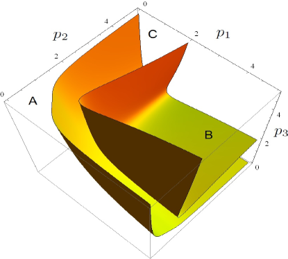
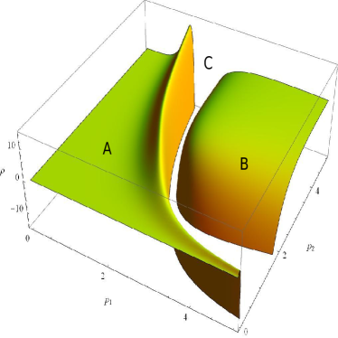
Figure 1: Left, zero surfaces of the maximum allowed density. Right, maximum allowed density vs. $p_{1}$ and $p_{2}$ where $p_{3}=p_{1}$. Both in Planck units.

Although the effective Hamiltonian without inverse triad correction Ed-BIX reduces to the effective Hamiltonian for closed FLRW model with less correction closed , because of the presence of the effects from the operators $\widehat{|p_{i}|^{-1/4}}$ and its positive powers in the curvature term of the Hamiltonian, this property no longer holds for the modified Hamiltonian Eq.(36) and the closed FLRW model effective Hamiltonian with inverse triad correction is not a reduction of this modified Hamiltonian.

IV.1 A different choice: Bianchi IX reduces to FLRW k=1

As we mentioned before, the Bianchi IX effective theory with inverse triad corrections does not reduce to the closed FLRW model. However, by keeping the effects of operator $\hat{A}$ and neglecting the other corrections in the gravitational part of the Hamiltonian constraint, one can construct a Bianchi IX effective theory which has some part of the inverse corrections and it does reduce to the closed FLRW model with inverse triad corrections. In this model, the Hamiltonian constraint is given by

$$\begin{split}\mathcal{H}_{eff}=&-\frac{V}{8\pi G\gamma^{2}\lambda^{2}}A(V)(\sin\bar{\mu}_{1}c_{1}\sin\bar{\mu}_{2}c_{2}+\sin\bar{\mu}_{1}c_{1}\sin\bar{\mu}_{3}c_{3}+\sin\bar{\mu}_{2}c_{2}\sin\bar{\mu}_{3}c_{3})\\ &+\frac{\sigma}{8\pi G\gamma^{2}\lambda}A(V)\left(\frac{p_{1}p_{2}}{p_{3}}\sin\bar{\mu}_{3}c_{3}+\frac{p_{2}p_{3}}{p_{1}}\sin\bar{\mu}_{1}c_{1}+\frac{p_{1}p_{3}}{p_{2}}\sin\bar{\mu}_{2}c_{2}\right)\\ &-\frac{\sigma^{2}(1+\gamma^{2})}{32\pi G\gamma^{2}}A(V)\left(2\frac{p_{1}^{3/2}}{\sqrt{p_{2}p_{3}}}+2\frac{p_{2}^{3/2}}{\sqrt{p_{1}p_{3}}}+2\frac{p_{3}^{3/2}}{\sqrt{p_{1}p_{2}}}-\frac{(p_{1}p_{2})^{3/2}}{p_{3}^{5/2}}-\frac{(p_{1}p_{3})^{3/2}}{p_{2}^{5/2}}-\frac{(p_{2}p_{3})^{3/2}}{p_{1}^{5/2}}\right)\\ &+U(\phi)V+\frac{1}{2V_{c}^{6}}p_{\phi}^{2}V^{2}h(V)^{6}\end{split}$$ (46)

$$\dot{p}_{1}=\frac{1}{\gamma\lambda}A(V)\cos\bar{\mu}_{1}c_{1}\left[p_{1}(\sin\bar{\mu}_{2}c_{2}+\sin\bar{\mu}_{3}c_{3})-\lambda\sigma\sqrt{\frac{p_{2}p_{3}}{p_{1}}}\right]$$ (47)

$$\begin{split}\dot{c_{1}}=&-\frac{1}{\gamma\lambda^{2}}\left(\frac{1}{2}\sqrt{\frac{p_{2}p_{3}}{p_{1}}}A(V)+A_{,p_{1}}V\right)\left(\sin\bar{\mu}_{1}c_{1}\sin\bar{\mu}_{2}c_{2}+\sin\bar{\mu}_{1}c_{1}\sin\bar{\mu}_{3}c_{3}+\sin\bar{\mu}_{2}c_{2}\sin\bar{\mu}_{3}c_{3}\right)\\ &-\frac{\sigma}{\lambda\gamma}\Bigg{(}\bigg{[}\frac{p_{2}p_{3}}{p_{1}^{2}}A(V)-\frac{p_{2}p_{3}}{p_{1}}A_{,p_{1}}\bigg{]}\sin\bar{\mu}_{1}c_{1}-\bigg{[}\frac{p_{3}}{p_{2}}A(V)+\frac{p_{1}p_{3}}{p_{2}}A_{,p_{1}}\bigg{]}\sin\bar{\mu}_{2}c_{2}\\ &-\bigg{[}\frac{p_{2}}{p_{3}}A(V)+\frac{p_{1}p_{2}}{p_{3}}A_{,p_{1}}\bigg{]}\sin\bar{\mu}_{3}c_{3}\Bigg{)}\\ &-A(V)\frac{c_{1}\cos\bar{\mu}_{1}c_{1}}{2\gamma\lambda}\left(-\frac{\lambda\sigma}{p_{1}}\sqrt{\frac{p_{2}p_{3}}{p_{1}}}+\sin\bar{\mu}_{2}c_{2}+\sin\bar{\mu}_{3}c_{3}\right)\\ &+A(V)\frac{c_{2}\cos\bar{\mu}_{2}c_{2}}{2\gamma\lambda\sqrt{p_{1}}}\left(-\lambda\sigma\sqrt{\frac{p_{3}}{p_{2}}}+\frac{p_{2}}{\sqrt{p_{1}}}\sin\bar{\mu}_{1}c_{1}+\frac{p_{2}}{\sqrt{p_{1}}}\sin\bar{\mu}_{3}c_{3}\right)\\ &+A(V)\frac{c_{3}\cos\bar{\mu}_{3}c_{3}}{2\gamma\lambda\sqrt{p_{1}}}\left(-\lambda\sigma\sqrt{\frac{p_{2}}{p_{3}}}+\frac{p_{3}}{\sqrt{p_{1}}}\sin\bar{\mu}_{1}c_{1}+\frac{p_{3}}{\sqrt{p_{1}}}\sin\bar{\mu}_{2}c_{2}\right)\\ &-A(V)\frac{\sigma^{2}(1+\gamma^{2})}{4\gamma}\left(\frac{5}{2}\frac{p_{2}^{3/2}p_{3}^{3/2}}{p_{1}^{7/2}}-\frac{1}{p_{1}^{3/2}\sqrt{p_{2}p_{3}}}(p_{2}^{2}+p_{3}^{2})-\frac{3\sqrt{p_{1}}}{2}(\frac{p_{2}^{3/2}}{p_{3}^{5/2}}+\frac{p_{3}^{3/2}}{p_{2}^{5/2}})+3\sqrt{\frac{p_{1}}{p_{2}p_{3}}}\right)\\ &+8\pi G\gamma\sqrt{\frac{p_{2}p_{3}}{p_{1}}}U(\phi)+\frac{4\pi G\gamma}{V_{c}^{6}}p_{\phi}^{2}h^{5}(V)\bigg{[}p_{2}p_{3}h(V)+6V^{2}h_{,p_{1}}\bigg{]}\end{split}$$ (48)

The expansion is

$$\begin{split}\theta=&\frac{1}{2\gamma\lambda}A(V)(\cos\bar{\mu}_{1}c_{1}\left[(\sin\bar{\mu}_{2}c_{2}+\sin\bar{\mu}_{3}c_{3})-\lambda\sigma\frac{1}{p_{1}}\sqrt{\frac{p_{2}p_{3}}{p_{1}}}\right]\\ &+\cos\bar{\mu}_{2}c_{2}\left[(\sin\bar{\mu}_{1}c_{1}+\sin\bar{\mu}_{3}c_{3})-\lambda\sigma\frac{1}{p_{2}}\sqrt{\frac{p_{1}p_{3}}{p_{2}}}\right]+\cos\bar{\mu}_{3}c_{3}\left[(\sin\bar{\mu}_{1}c_{1}+\sin\bar{\mu}_{2}c_{2})-\lambda\sigma\frac{1}{p_{3}}\sqrt{\frac{p_{1}p_{2}}{p_{3}}}\right])\end{split}$$ (49)

For large volume, the second term of $\dot{p}_{1}/p_{1}$ behaves like $\sqrt{p_{2}p_{3}}/p_{1}^{3/2}$ and in the limit of small volume behaves like $p_{2}p_{3}/p_{1}$. Since $p_{i}$’s can be small or large numbers, there is no bound for $\dot{p}_{1}/p_{1}$ and with similar arguments about unboundedness of $\dot{p}_{2}/p_{2}$ and $\dot{p}_{3}/p_{3}$, it can be proved that expansion is not bounded.

V discussion

This paper is the first in a series devoted to the study of the Bianchi IX model within LQC. In this contribution we introduced for the first time inverse corrections for Bianchi IX and explored some of its properties. In particular we have studied the effective theory that follows from the quantum theory and have considered the behaviour of several geometric scalars. This is important to study singularity resolution within LQC. Some of these questions are explored in the second paper of this series CM-BIX , where numerical solutions to the effective equations with a massless scalar field are studied.

In the study of the behaviour of expansion and shear for the effective theory, we have shown that these scalars are not absolutely bounded, which might be a signal that the quantization is problematic cs:unique . However, when one takes into account some energy conditions, one learns that the allowed region where solutions to the effective equations can be, becomes disconnected. There are two allowed regions and the solutions have to lie within one of them. The region where the would be singularity lies, and where large anisotropies are allowed, is disconnected from the region with large volume. Thus, any realistic universe that reaches large volume at recollapse can not reach that region, and it can, at most, have a finite number of oscillations. Thus, one might expect that loop quantum corrections to the dynamics have an important effect on the avoidance, not only of the singularity, but of the mixmaster behaviour that is so characteristic of the classical dynamics. This and other issues will be studied in more detail in the third paper of the series CKM-2 .

References

• (1) A. Ashtekar and P. Singh, “Loop Quantum Cosmology: A Status Report,” Class. Quant. Grav.  28 (2011) 213001 arXiv:1108.0893v2 [gr-qc]; I. Agullo and A. Corichi, “Loop Quantum Cosmology,” arXiv:1302.3833 [gr-qc].
• (2) A. Ashtekar, T. Pawlowski and P. Singh, “Quantum nature of the big bang: Improved dynamics,” Phys. Rev. D 74, 084003 (2006) arXiv:gr-qc/0607039.
• (3) A. Ashtekar, A. Corichi and P. Singh, “Robustness of key features of loop quantum cosmology,” Phys. Rev. D 77, 024046 (2008). arXiv:0710.3565 [gr-qc].
• (4) A. Corichi and E. Montoya, “On the Semiclassical Limit of Loop Quantum Cosmology,” Int. J. Mod. Phys. D 21, 1250076 (2012) [arXiv:1105.2804 [gr-qc]]; A. Corichi and E. Montoya, “Coherent semiclassical states for loop quantum cosmology,” Phys. Rev. D 84, 044021 (2011) [arXiv:1105.5081 [gr-qc]].
• (5) P. Diener, B. Gupt and P. Singh, “Numerical simulations of a loop quantum cosmos: robustness of the quantum bounce and the validity of effective dynamics,” Class. Quant. Grav.  31, 105015 (2014) [arXiv:1402.6613 [gr-qc]].
• (6) P. Singh, “Are loop quantum cosmos never singular?,” Class. Quant. Grav.  26, 125005 (2009) [arXiv:0901.2750 [gr-qc]].
• (7) A. Corichi and P. Singh, “Is loop quantization in cosmology unique?,” Phys. Rev.  D 78, 024034 (2008) arXiv:0805.0136 [gr-qc]; “A geometric perspective on singularity resolution and uniqueness in loop quantum cosmology,” Phys. Rev.  D 80, 044024 (2009) arXiv:0905.4949 [gr-qc].
• (8) L. Szulc, W. Kaminsk and J. Lewandowski, “Closed FRW model in Loop Quantum Cosmology,” Class. Quant. Grav. 24 (2007) 2621.A. Ashtekar, T. Pawlowski, P. Singh, and K. Vandersloot, “Loop quantum cosmology of k=1 FRW models,” Phys. Rev. D 75 (2007) 024035.
• (9) A. Corichi and A. Karami, “Loop quantum cosmology of k=1 FRW: A tale of two bounces”, Phys. Rev. D 84:044003 (2011), arXiv:1105.3724 [gr-qc].
• (10) A. Corichi and A. Karami, “Loop quantum cosmology of k = 1 FLRW: Effects of inverse volume corrections,” Class. Quant. Grav.  31, 035008 (2014) arXiv:1307.7189 [gr-qc].
• (11) P. Singh and F. Vidotto, “Exotic singularities and spatially curved Loop Quantum Cosmology,” Phys. Rev. D 83, 064027 (2011) [arXiv:1012.1307 [gr-qc]].
• (12) V. A. Belinskii, I. M. Khalatnikov, and E. M. Lifshitz, “Oscillatory approach to a singular point in relativistic cosmology”, Adv. Phys. 19, 525 (1970).
• (13) V. A. Belinskii, I. M. Khalatnikov, and E. M. Lifshitz, “A general solution of the Einstein equations with a time singularity”, Adv. Phys. 31, 639 (1982).
• (14) A. Ashtekar, A. Henderson and D. Sloan, “A Hamiltonian Formulation of the BKL Conjecture,” Phys. Rev.  D 83, 084024 (2011) arXiv:1102.3474 [gr-qc].
• (15) K. C. Jacobs, “Spatially homogeneous and euclidean cosmological models with shear,” Astrophys. J. 153 (1968) 661.
• (16) J. Wainwright, G. F. R. Ellis, Dynamical Systems in Cosmology, Cambridge University Press (1997).
• (17) T. Thiemann, “Quantum spin dynamics (QSD),” Class. Quant. Grav.  15, 839 (1998) [gr-qc/9606089].
• (18) A. Ashtekar, A. Corichi and J. A. Zapata, “Quantum theory of geometry III: Noncommutativity of Riemannian structures,” Class. Quant. Grav.  15, 2955 (1998) [gr-qc/9806041].
• (19) D. W. Chiou and K. Vandersloot, “The behavior of non-linear anisotropies in bouncing Bianchi I models of loop quantum cosmology,” Phys. Rev.  D 76, 084015 (2007) arXiv:0707.2548 [gr-qc]; D. W. Chiou, “Effective Dynamics, Big Bounces and Scaling Symmetry in Bianchi Type I Loop Quantum Cosmology,” Phys. Rev.  D 76, 124037 (2007). arXiv:0710.0416 [gr-qc].
• (20) Ashtekar, A. and Wilson-Ewing, E., “Loop quantum cosmology of Bianchi I models”, Phys. Rev. D, 79, 083535, (2009).
• (21) P. Singh, “Curvature invariants, geodesics and the strength of singularities in Bianchi-I loop quantum cosmology”, Phys.Rev., D85, 104011,(2012).
• (22) Ashtekar, A. and Wilson-Ewing, E., “Loop quantum cosmology of Bianchi type II models”, Phys. Rev. D, 80, 123532, (2009).
• (23) A. Corichi and E. Montoya, “Effective Dynamics in Bianchi Type II Loop Quantum Cosmology”, Phys. Rev. D, 85, 104052, (2012). arXiv:1201.4853; A. Corichi and E. Montoya, “Qualitative effective dynamics in Bianchi II loop quantum cosmology,” AIP Conf. Proc.  1473, 113 (2011).
• (24) Wilson-Ewing, E., “Loop quantum cosmology of Bianchi type IX models”, Phys. Rev. D, 82, 043508, (2010).
• (25) P. Singh and E. Wilson-Ewing, “Quantization ambiguities and bounds on geometric scalars in anisotropic loop quantum cosmology”, Class. Quant. Grav.  31 (2014) 035010, arXiv:1310.6728 [gr-qc].
• (26) B. Gupt and P. Singh, “Contrasting features of anisotropic loop quantum cosmologies: The Role of spatial curvature,” Phys. Rev. D 85, 044011 (2012) [arXiv:1109.6636 [gr-qc]].
• (27) A. Corichi and E. Montoya, “Loop quantum cosmology of Bianchi IX: Effective dynamics,” arXiv:1502.02342 [gr-qc].
• (28) A. Corichi, A. Karami and E. Montoya, in preparation (2016).
• (29) A. Corichi, A. Karami and E. Montoya, “Loop Quantum Cosmology: Anisotropy and singularity resolution,” Springer Proc. Phys.  157, 573 (2014). arXiv:1210.7248 [gr-qc].