On the Vortex Dynamics in Fractal Fourier Turbulence

Abstract

Incompressible, homogeneous and isotropic turbulence is studied by solving the Navier-Stokes equations on a reduced set of Fourier modes, belonging to a fractal set of dimension $D$. By tuning the fractal dimension parameter, we study the dynamical effects of Fourier decimation on the vortex stretching mechanism and on the statistics of the velocity and the velocity gradient tensor. In particular, we show that as we move from $D=3$ to $D\sim 2.8$, the statistics gradually turns into a purely Gaussian one. This result suggests that even a mild fractal mode reduction strongly depletes the stretching properties of the non-linear term of the Navier-Stokes equations and suppresses anomalous fluctuations.

1 Introduction

A distinctive feature of three-dimensional fully developed turbulent flows is the presence of bursty fluctuations in the velocity increment statistics over a wide range of scales, a phenomenon called intermittency frisch . The statistical signature of such fluctuations is the violation of the self-similar Kolmogorov theory in the inertial range of scales.
While Eulerian frisch ; Arneodo1996 ; Sreeni1997 and Lagrangian Mo2001 ; PoF2005 ; Xu2006 ; PRL2008 ; rev_toschi_bode observations leave no doubt about the existence of intermittency, a theoretical framework explaining its origin and its relation to the direct cascade of kinetic energy is still lacking. The question is fundamental frisch ; Kr71 ; Kr74 and practical since modeling relies on assumptions invoking scaling invariance and scale-by-scale energy budgets MK00 ; SreFa06 . During the formation of strong fluctuations, large spatial structures create thin vorticity layers or filaments under both the action of shearing and stretching. Vortex stretching is essentially a process of interaction of vorticity and strain and is an important mechanism for understanding both intermittency as well as energy cascade in a turbulent flow frisch ; T99 . Its role can be quantified in experiments and numerical simulations, while closure approximations K61 ; orszag77 as well as phenomenological models frisch for homogeneous and isotropic turbulence fail to account for vortex structures.
In this paper, we propose to further investigate the relation between intermittency and vortex stretching by a novel approach to three dimensional turbulence. This consists in numerically solving the Navier-Stokes equations on a multiscale sub-set of Fourier modes (also dubbed Fourier skeleton), belonging to a fractal set of dimension $D\leq 3$ frisch2012 ; LBBMT2015 . For $D=3$, the original problem is recovered. This implies that the velocity field is embedded in a three dimensional space, but effectively possesses a number of Fourier modes that grows slower as $D$ decreases: in particular, in the Fourier space the number degrees of freedom inside a sphere of radius $k$ goes as $\#_{dof}(k)\sim k^{D}$.
Attempts to study homogeneous and isotropic $D$-dimensional turbulence, with $2\leq D\leq 3$, are not new (see FF1978 ), and were mostly inspired by statistical mechanics approaches to hydrodynamics: the idea is to find non-integer dimensions where closures, compatible with Kolmogrov 1941 theory, can be satisfactorily used. Equilibrium statistical mechanics in relation to Galerkin-truncated, three-dimensional Euler equations has been also used to study three-dimensional turbulence (see pioneering works by Lee Lee and Hopf Hopf ). In particular, recent numerics brachet2005 ) of the Euler eq. with a large but finite number of Fourier modes has interestingly shown that in the relaxation towards the equilibrium spectrum, large-scale dynamics exhibits a Kolmogorov spectrum. This suggests that relevant features of the turbulent cascade can be studied in terms of the thermalization mechanism ray2015 .
In frisch2012 , the idea of Galerkin truncation was adopted to investigate, in two-dimensional turbulence, the link between the inverse energy cascade and quasi-equilibrium Gibbs states with Kolmogorov spectrum, when the dynamics is restricted on a fractal set with $D=4/3$ lvov . Finally, the idea of changing the ”effective dimension” between $D=2$ and $D=3$ has been explored within shell models of turbulence, by modifying the conserved quantities of the system GJY2002 .
More recently, in LBBMT2015 , fractally Fourier decimated Navier-Stokes equations were studied for the first time in the range $2.5\leq D\leq 3$. Two main results emerged: (i) average fluctuations are mildly affected by the decimation, since the kinetic energy spectrum exponent gets a correction linear in the codimension $3-D$, i.e. $E^{D}(k)\propto k^{-5/3+(3-D)}$; (ii) differently, large fluctuations are severely modified, since the probability density function (PDF) of the vorticity becomes almost Gaussian already at $D=2.8$.
Here, we study more extensively the velocity increment statistics, and the vortex streching mechanism, as quantified by the statistics of second and third order invariants of the velocity gradients tensor. We show that it is significantly changed as we move from $D=3$ to $D=2.5$, with the evidence of the intermittent behaviour almost vanishing even for a tiny decimation, i.e., for $D\simeq 2.98$. This leaves a distictive mark on the vorticity field: the filamentary structure at $D=3$ is replaced by a proliferation of small grains of vorticity populating all regions of the flow (as shown in Figure 1).
In Section 2, we describe the equations and numerical methods used to generate the dataset, as well the statistical approach adopted to analyse it. In Section 3, we first discuss few results about the statistical behaviour of velocity fluctuations and the spectral properties of Fourier decimated turbulence. Then, we focus on the small-scale statistics by analysing the velocity gradient tensor statistics. Finally we provide some conclusions in Section 4.

$D$	$3$	$3$	$2.999$	$2.99$	$2.99$	$2.98$	$2.98$	$2.8$	$2.8$	$2.5$	$2.5$
$N$	$1024$	$1024$	$1024$	$1024{\it(*)}$	$2048$	$1024$	$2048$	$1024$	$1024$	$1024$	$1024{\it(*)}$
$\nu$	$6.e-4$	$8.e-4$	$6.e-4$	$6.e-4$	$2.e-4$	$6.e-4$	$2.e-4$	$6.e-4$	$8.e-4$	$6.e-4$	$1.5e-4$
$M_{r}$	$100\%$	$100\%$	$99\%$	$93\%$	$92\%$	$87\%$	$85\%$	$25\%$	$25\%$	$3\%$	$3\%$
$\eta$	$0.75$	$0.95$	$0.75$	$0.95$	$0.70$	$0.75$	$0.70$	$0.40$	$0.90$	$0.65$	$0.2$
${\cal N}_{T}$	$10$	$10$	$10$	$11$	$10$	$11$	$7$	$10$	$10$	$10$	$10$

Table 1: Direct Numerical Simulation parameters. The fractal dimension $D$; the grid resolution per spatial direction $N$; the viscosity $\nu$; the percentage $M_{r}$ of Fourier modes that survives to the decimation action; Kolmogorov length scale $\eta$ in grid spacing units, where the grid spacing is $\Delta x=2\pi/N$; the number of steady state large-scale eddy-turnover-times collected for statistical analysis, ${\cal N}_{T}$. For all simulations, $L=2\pi$ is the size of the system. Runs labeled with an asterisk (*) have been performed with two different realisations of the fractal mask. Note that the reference wavenumber $k_{0}$ entering the definition of the probability, $h_{k}=(k/k0)^{D−3}$, is eual to 1.

2 Model Equations and Methods

2.1 The Navier-Stokes equations on a Fractal Fourier set

Let us define ${\bf v}({\bf x},t)$ and $\hat{{\bf u}}({\bf k},t)$ as the real and Fourier space representation of the velocity field in $D=3$, respectively. We then introduce a decimation operator ${\cal P}^{D}$ that acts on the velocity field as:

$${\bf v}^{D}({\bf x},t)={\cal P}^{D}{\bf v}({\bf x},t)=\sum_{{\bf k}\in{\cal Z}^{3}}e^{i{\bf k\cdot x}}\,\gamma_{\bf k}\hat{{\bf u}}({\bf k},t)\,.$$ (1)

Here ${\bf v}^{D}({\bf x},t)$ is the decimated velocity field.
In this equation $\gamma_{{\bf k}}$ represent random numbers that are quenched in time and are determined as :

$$\gamma_{\bf k}=\begin{cases}1,&\text{with probability}\ h_{k}\,,\\ 0,&\text{with probability}\ 1-h_{k},k\equiv|{\bf k}|\,.\end{cases}$$ (2)

The choice for the probability $h_{k}\propto(k/k_{0})^{D-3}$, with $0<D\leq 3$ and $k_{0}$ a reference wavenumber, ensures that the dynamics is isotropically decimated to a $D$-dimensional Fourier set. The factors $h_{k}$ are chosen independently and preserve Hermitian symmetry $\gamma_{k}=\gamma_{-k}$ so that ${\cal P}^{D}$ is self-adjoint as was described in frisch2012 . The Navier-Stokes equations for the decimated velocity field ${\bf v}^{D}({\bf x},t)$ are then defined as:

$$\partial_{t}{\bf v}^{D}={\cal P}^{D}N({\bf v}^{D},{\bf v}^{D})+\nu\,\nabla^{2}{\bf v}^{D}+{\bf F}^{D}\,.$$ (3)

Here $N({\bf v},{\bf v})=-{\bf v}\cdot{\bf{\nabla v}}+{\bf\nabla}p$ is the non-linear term of the NS equation. Equation  3 conserves both energy and helicity in the inviscid and unforced limit, exactly as in the original (non decimated) problem with $D=3$; ${\bf F}^{D}$ is the large-scale forcing, injecting kinetic energy in the system. The notation above, ${\cal P}^{D}N({\bf v}^{D},{\bf v}^{D})$, is to imply the fact that the non-linear term is projected, at every time iteration, on the quenched fractal set, so that its dynamical evolution remains on the same Fourier skeleton at all times. Similarly, the initial condition and the external forcing are defined on the same fractal set of Fourier modes.
In the sequel, for the sake of simplicity, we shortly refer to ${\bf v}({\bf x})$ and $\hat{{\bf v}}({\bf k})$ as the real and Fourier space representation of the solution of the decimated Navier-Stokes equations (3).

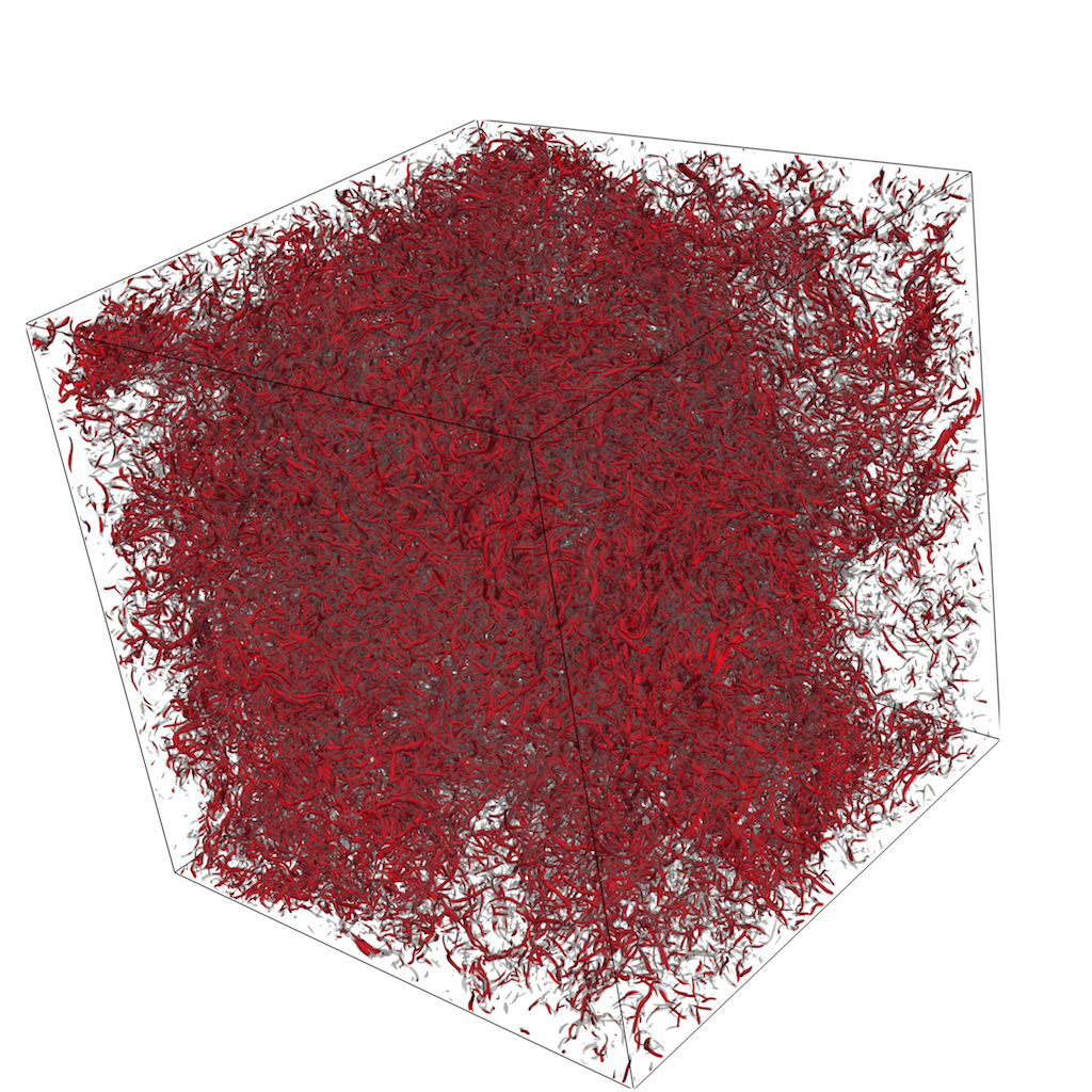
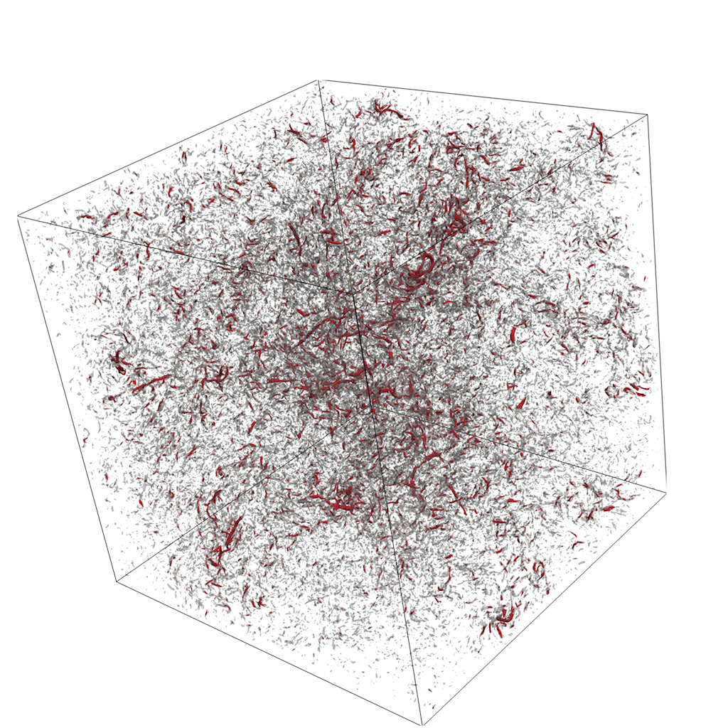
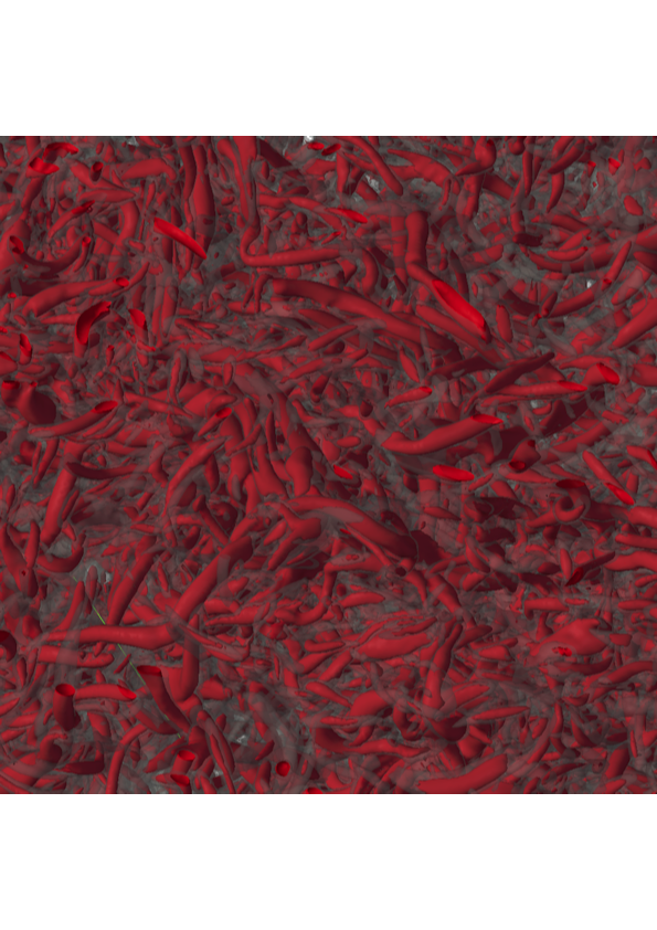
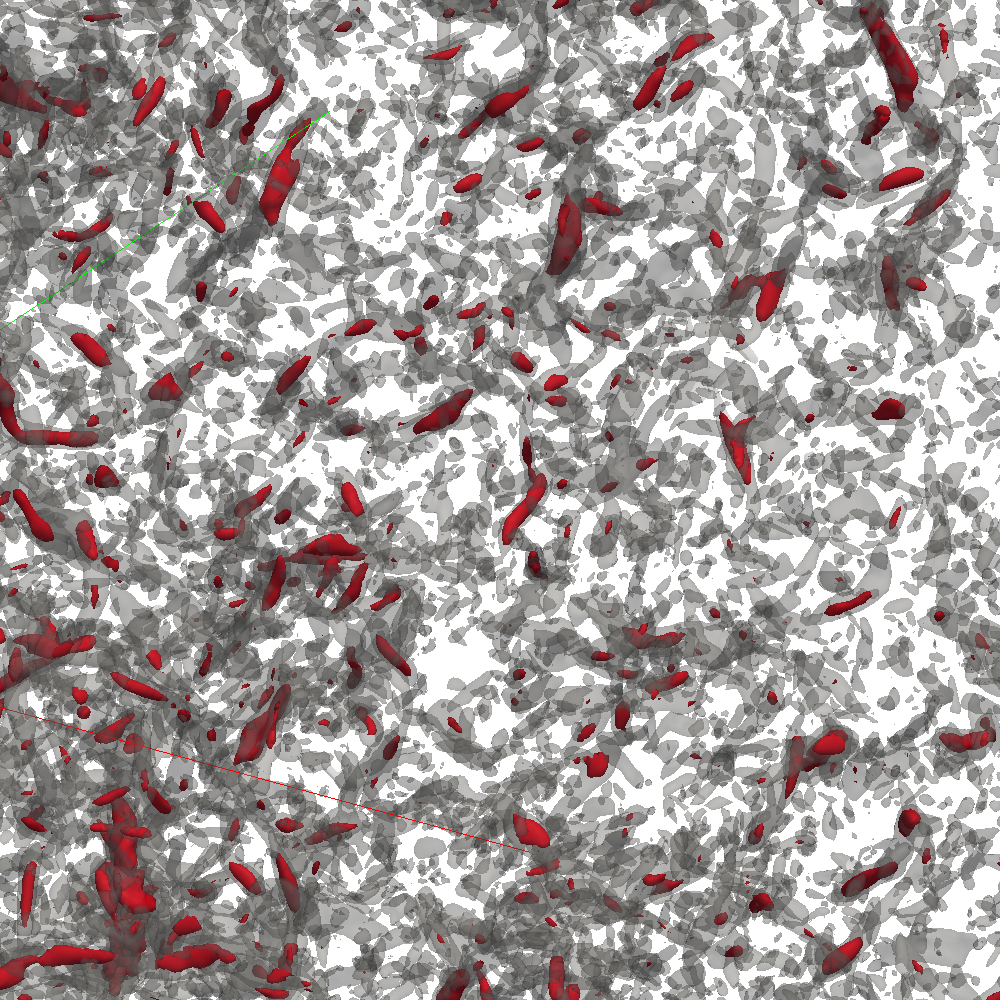
Figure 1: Plot of the most intense vortical structures. (top) A snapshot of the turbulent flow with $D=3$ (left) and with $D=2.98$ (right). Isosurfaces of the $Q$ invariant (see text) of the velocity gradient tensor are plotted: values $Q/Q_{rms}=1$ (grey) and $Q/Q_{rms}=2$ (red). (bottom) A zoom in the top snapshots highlights details of the small scales. Data refer to runs with $N=1024$.

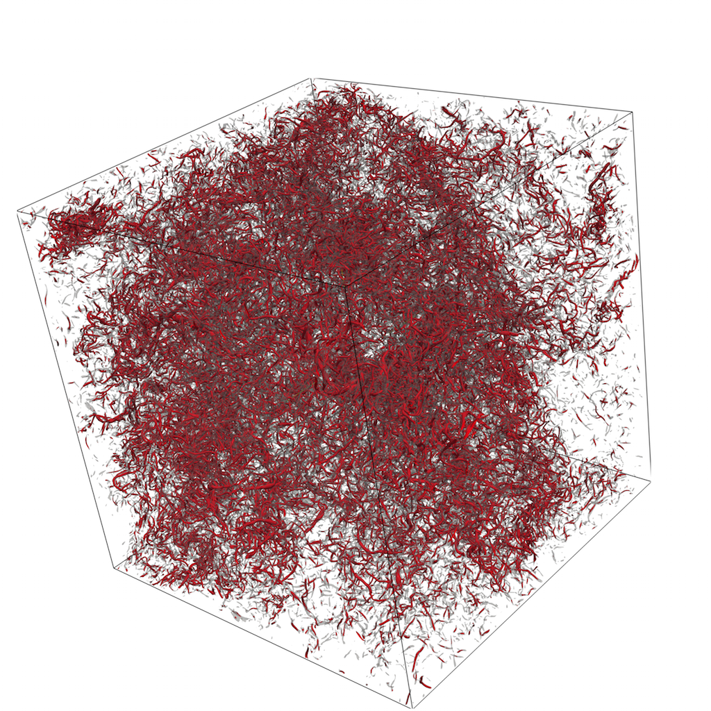
Figure 2: Isosurfaces of the $Q$ invariant as above. Here we show what is left of the turbulent flow with $D=3$ ($N=1024$), after applying the static mask with dimension $2.98$. The full volume on the left; a zoom highlighting small-scale features, on the right.

2.2 Direct Numerical Simulations Set-up

We solved equations (3) on a regular, periodic volume with $N=1024^{3}$ and $2048^{3}$ grid points, by adopting a standard pseudo-spectral approach fully dealiased with the two-thirds rule; time stepping is done with a second-order Adams-Bashforth scheme. A large-scale forcing ${\bf F}$ keeps the total kinetic energy constant in a range of shells, $0.7\leq|{\bf k}|<1.7$, leading to a statistically stationary, homogeneous and isotropic flow pope . For each run, we generated a mask, that is kept quenched throughout the numerical simulation. We performed several runs at changing the fractal dimension $2.5\leq D\leq 3$, the spatial resolution, the viscosity and also the realization of the fractal quenched mask. The case for $D=3$ is also referred as standard case. We summarise in Table1 the relevant parameters of the numerical experiments performed.
We mention that an a posteriori projection on a set of fractal dimension $D$ can also be obtained by applying, in Fourier space, the mask on snapshots of the velocity field which is solution of the original three-dimensional Navier-Stokes equations. This is a static fractal Fourier decimation, whose effect can be compared to that of the dynamical decimation, in the statistical analysis.

3 Results and Discussion

We start our analysis by considering a visualisation of the most intense vortical structures, revealing the effect of decimation on turbulent flows. In Figure 1, we plot isosurfaces of the $Q=Tr[{\bf A}^{2}]$ invariant of the velocity gradient tensor, $A_{ij}=\partial_{i}v_{j}$. The Q-criterion is based on the observation that

$$Q=\frac{1}{2}(\Omega_{ij}\Omega_{ij}-S_{ij}S_{ij});$$

where the vorticity tensor is $\Omega_{ij}=1/2(\partial_{i}v_{j}-\partial_{j}v_{i})$ and the rate-of-strain tensor is $S_{ij}=1/2(\partial_{i}v_{j}+\partial_{j}v_{i})$. Therefore, flow regions where $Q$ is positive identify positions where the strength of rotation overcomes strain. These are the best candidates to be considered as vortex iso-surfaces Dubief . From Figure 1, we see that the $D=3$ case shows a large number of structures of both large and small-scale vortex filaments. The decimated case with $D=2.98$ clearly differs because structures are smaller and less elongated, also they are much less abundant, indicating a less intermittent spatial distribution of structures. We stress that fractal decimation has non-trivial dynamical effect, which differs from the simple action of a vector projection in Fourier space. To make this immediately clear, we plot in Figure 2 the $Q$ isosurfaces obtained after applying the a posteriori, static mask of dimension $D=2.98$ on the $D=3$ turbulent velocity field. While the static decimation simply removes velocity fluctuations at specific wavenumbers, the dynamical action of the Fourier decimation provokes a complete reorganization of the flow structures.

Figure 3: (Main body) The lin-log plot of the probability density function of the spectral flux $P(\Pi(k))$, normalised to unitary area, for runs with different $D$; resolution is $N=1024$. (Inset) the comparison of the spectral fluxes obtained at the two resolutions, $N=1024$ and $N=2048$, and for different fractal dimensions $D$.

3.1 Velocity field statistics

We consider the statistics of mean turbulent fluctuations by analysing the spectral behaviour of the kinetic energy spectrum and energy flux, when the fractal dimension $D$ is varied.

Figure 4: Log-log plot of the compensated kinetic energy spectra, $E(k)\,k^{5/3-(3-D)}$, obtained at the two resolutions, $N=1024$ and $N=2048$, and for different fractal dimensions $D$. We only report those cases for which the linear correction to the exponent, due to the fractal decimation, is appreciable. At resolution $N=1024$, for $D=2.5$ label $m1$ and $m2$ indicate two sets of numerical simulations with different masks. At resolution $N=1024$, for $D=2.8$, label $\nu_{1}$ and $\nu_{2}$ indicate runs with different viscosities equal to $6.e-4$ and $8.e-4$, respectively: for these runs the masks are also different.

From the DNS data, the energy spectrum is measured by angular averages on Fourier-space unitary shells,

$$E^{D}(k)\equiv\sum_{k\leq|{\bf k}|\leq k+1}\langle v_{i}({\bf k})v_{i}({\bf k})^{*}\rangle\,,$$ (4)

where the asterisk is for complex conjugation. The energy flux $\Pi^{D}(k)$ through wavenumber $k$ due to the nonlinear transfer is measured as

$$\Pi^{D}(k)\equiv\sum_{|{\bf q}|<k}\sum_{{\bf p}}\langle{\bf v}^{*}(-{\bf q}-{\bf p})\cdot\left[{\bf q}\cdot({\bf v}({\bf q}){\bf v}({\bf p}))\right]\rangle\,.$$ (5)

As reported in LBBMT2015 , a dimensional argument can be built up to quantify possible modification of the exponent of the kinetic energy spectrum due to fractal decimation. It relies on two assumptions: (i) scaling invariance of the velocity fluctuations in the inertial range of scales; (ii) the existence of a constant (k-independent) spectral energy flux in the inertial range. We give the former for granted, since intermittency manifests only in terms of a tiny anomalous correction in the energy spectrum of three-dimensional turbulence IsGoKa09 .

Figure 5: (Main body) Log-log plot of the longitudinal second order structure function for different fractal dimensions $D$. Data are at resolution $N=1024$. (Inset) Log-lin plot of the local slopes in ESS of the 4th-order longitudinal (filled circles) and transverse (filled boxes) structure functions in terms of the second order one, versus the separation scale $r$. Color symbols are the same of the main body: lower curves are for $D=3$, middle curves for $D=2.99$ and upper curves for $D=2.98$.

As for the latter, we plot in the inset Figure 3, the kinetic energy flux $\Pi(k)$ through wavenumber $k$ for DNS with different fractal decimation $D$, and for both resolutions. It is clear that even in the presence of a strong reduction of degrees of freedom, an average constant flux in Fourier space is observed and a cascade of kinetic energy takes place.
We also quantify the fluctuations in the Fourier space energy transfer, by plotting in Figure 3 the probability density function of the spectral flux. The PDF is calculated measuring the fluctuations of $\Pi(k)$ for wave-numbers in a limited range $k\in[3:30]$, corresponding to the constant transfer region where the flux has a plateau. We can observe that the fluctuations of the spectral transfer tend to be of the same amplitude, when $D$ is changed. Only for the case of a very strong decimation with $D=2.5$, we notice the presence of slightly larger fluctuations due to the fact the number of triads in the dynamical process are less and less as $D$ increases.

Figure 6: Log-lin plot of the normalised drag reduction coefficient $f/f_{D=3}$ versus the dimension deficit $3-D$. Error bars are estimated from statistical fluctuations.

Figure 4 shows the compensated kinetic energy spectra, $E(k)k^{5/3-(3-D)}$: fractal decimation acts to make the spectrum shallower, and the correction is small, being linear in the dimension deficit $3-D$ LBBMT2015 . Such correction is clearly negligible for those runs at $D\in[2.98,3)$, but starts to be appreciable at $D=2.8$. At $D=7/3$ the spectrum would in principle become divergent at small wavenumbers. However at such fractal dimension, about less than $1\%$ of the modes would survive for the present resolutions, almost annihilating the role of the non-linear transfer and making the energy dissipation almost in a direct balance with the energy injection. We note that, recently, the Burgers equation decimated on a fractal Fourier set of dimension $D\leq 1$ was numerically studied BBFR2016 . Results obtained at fixed $D$ and for larger and larger values of the Reynolds number, suggest that Fourier decimation is a singular perturbation for the spectral scaling properties. Should this happen for the Navier-Stokes equations also, it is something to explore.
It is also important to notice that fractal Fourier decimation has a strong effect on the vortex stretching mechanism: this implies that the energy bottlenecks F1994 ; Lohse1995 ; Frisch2008 , generally observed at high Reynolds numbers in $D=3$ turbulence, might become less and less important for $D<3$.

We now consider the Fourier transform of the energy spectrum, giving the second order velocity longitudinal structure function $S^{(2)}_{L}\equiv\langle[({\bf v}({\bf x}+{\bf r})-{\bf v}(x))\cdot\hat{{\bf r}}]^{2}\rangle$. This is plotted in Figure 5. By decreasing the fractal dimension $D$, the curves become less and less steep approaching the Kolmogorov dimensional scaling $S^{(2)}_{L}\simeq(r/L)^{\zeta_{2}}$, linearly corrected by the dimension deficit $\zeta_{2}=2/3-(3-D)$. Note that the run at $D=2.5$ has a smaller kinematic viscosity, hence a larger kinetic energy.

Figure 7: Isosurfaces of the joint probability density function $P(Q^{*},R^{*})$, where $Q^{*}=Q/\langle Q^{2}\rangle^{1/2}$ and $R^{*}=R/\langle Q^{2}\rangle^{3/2}$. Isosurfaces are equispaced logarithmically. Note that when the fractal dimension $D$ is lowered, the range of fluctuations for the $Q-R$ variables is substantially modified, and become much smaller. The black line is the Viellefosse line $L\equiv 27/4R^{2}-Q^{3}=0$.

It is interesting to check how longitudinal and trasversal structure functions approach the dimensional scaling. Indeed it has been observed that, in statistically homogeneous and isotropic turbulence, longitudinal and trasversal structure functions do have different anomalous corrections PhysD2008 , contrary to what would be expected on the basis of symmetry arguments BifProc2005 . Whether this is an effect due to finite-Reynolds numbers or not remains an open issue. In the inset of Figure 5, we plot the local slopes of the longitudinal and transverse fourth order structure functions, by using the so-called extended self-similarity technique (ESS)ess (see also ray2010 for a recent discussion of the topic). To be more precise, we consider the ratio of the scaling exponent of the fourth order longitudinal (transverse) structure function to that of the second order longitudinal (transverse) one:

$$\frac{\zeta_{4}}{\zeta_{2}}(r)=\frac{d\log S^{(4)}_{L,T}(r)}{d\log S^{(2)}_{L,T}(r)}\,,$$ (6)

where the longitudinal structure functions are $S^{(n)}_{L}(r)\equiv\langle[\delta_{r}{{\bf v}}\cdot\hat{\bf r}]^{n}\rangle$ with $\delta_{r}{{\bf v}}={{\bf v}}({{\bf r}})-{{\bf v}}(0)$, and the purely transverse structure functions are $S^{(n)}_{T}(r)\equiv\langle[\delta_{r}v(\hat{{\bf r}}_{T})]^{n}\rangle$ and $\hat{{\bf r}}_{T}\cdot{\bf v}=0$. For $D=3$, the curve for the transverse structure function is well below that of the longitudinal one, hence the anomalous correction is larger for the former than for the latter Gotoh2002 ; Benzi2010 . When the fractal dimension is decreased, $D<3$, such difference also diminishes but the two curves remain separated even when approaching Gaussianity. This might suggest that such difference in the standard $D=3$ turbulence is not due to finite Reynolds effects but it is genuine, and different anomalous corrections characterize longitudinal and transverse structure functions.

A different way to quantify the effects of fractal decimation, beyond scaling properties, is to look at the ratio of the kinetic energy input to the resulting kinetic energy throughput in the turbulent flow. An adimensional measure can be defined as BCM2005

$$f_{d}\equiv\frac{F\,L}{\langle v\rangle^{2}}=\frac{2\epsilon L}{v^{3}_{rms}}\,$$ (7)

where $F$ quantifies the amplitude of the external forcing and $L$ is the large-scale of the flow; moreover from the definition of the energy input $\epsilon\equiv 1/2\langle{\bf F}\cdot{\bf v}\rangle$ we have the dimensional relation $F\simeq 2\epsilon/\langle v^{2}\rangle^{1/2}$. In this terms, $f_{d}$ is a drag coefficient which can be measured when the fractal dimension is varied. From the results plotted in Figure 6, it appears that fractal decimation reduces the drag in the flow with respect to the standard case with $D=3$. Moreover there is a Reynolds dependence: we observe a larger reduction for larger Reynolds numbers. This sort of drag reduction is accompanied, as we will see below, by a restructuring of the flow, since regions characterised by intense vortical stretching almost disappear as $D$ is decreased.

3.2 Velocity gradient tensor statistics

As discussed before, the vortex stretching mechanism can be quantified by measuring the statistical behaviour of the invariants of velocity gradient tensor ${\cal{\bf A}}_{ij}=\partial v_{i}/\partial x_{j}$ (for a detailed discussion, see CPC ; BMC ). The characteristic equation $det({\cal{\bf A}}-\lambda{\cal{\bf I}})=0$ can be written as:

$$\lambda^{3}+P\lambda^{2}+Q\lambda+R=0\,.$$ (8)

For an incompressible flow, of the three tensor invariants only two are different from zero: $Q=-1/2tr[{\cal{\bf A}}^{2}]$ and $R=-1/3tr[{\cal{\bf A}}^{3}]$.
From previous experimental Tao2002 ; Luthi2005 and numerical Martin1998 studies in three-dimensional homogeneous and isotropic turbulence, some general geometric features of the tensor have been highlighted. These are: the vorticity vector is preferentially aligned with the eigenvector associated to the intermediate eigenvalue of the strain-rate tensor ${\cal{\bf S}}$; there are two positive and one negative eigenvalues of the rate-of-strain, ${\cal{\bf S}}$, such that the associated local flow structure is an axisymmetric extension; the joint probability distribution of the two invariants, $P(Q,R)$, has a typical teardrop shape extending around the so-called zero-discriminant or Vieillefosse line $L\equiv 27/4R^{2}+Q^{3}=0$ viellefosse . The Viellefosse line divides the $Q-R$ plane in two different regions depending whether the velocity gradient tensor has three real eigenvalues with $L<0$, or two complex-conjugate and one real eigenvalues, with $L>0$. This means that $L>0$ is the region where vorticity is dominant; the region $L<0$ is strain-dominated region. The upper left region (with $L>0$, and one positive real eingenvalue and two complex-conjugates ones) is the statistical signature of the vortex stretching dominating the turbulent flow, while long right tail in the lower right side ($L<0$ and two positive and one negative real eingenvalues) is associated with intense elongational strain.
In the original $D=3$ problem, the temporal evolution of the velocity gradient tensor is also of particular interest beyond the geometrical properties. Indeed a set of exact equations viellefosse ; cantwell1992 , although not closed, can be derived taking the gradient of Navier-Stokes equations. By doing so, the equations for the Lagrangian evolution of the gradient tensor components is

$$d{\cal A}_{ij}/dt=-{\cal A}_{ik}{\cal A}_{kj}-\partial_{ij}p+\nu\partial^{2}{\cal A}_{ij}\,,$$ (9)

where $p$ is the pressure divided by the fluid density. The need of a closure comes from the fact that both the pressure hessian and the viscous terms are not simply known in terms of ${\bf A}$. Such a set of equations, which gives insight on the small-scale intermittency, has been largely investigated, and different model closures have been proposed viellefosse ; Girimaji1990 ; CPS1999 ; Chevillard2006 ; Chevillard2008 .
In the case of fractal Fourier Navier-Stokes equations, the situation is however different. Because of the presence of the decimation projector in the non-linear term, the structure of the equation of motion in terms of the material derivative is broken. Hence, any closure model based on the lagrangian evolution of the velocity gradient tensor is ruled out.
In Figure7, we plot the joint distribution of the velocity gradient tensor invariants, $P(Q,R)$ for data at $N=1024$, since the dataset is richer. As the fractal dimension $D$ decreases, the joint probability looses its asymmetric shape, and become more and more centered. Moreover extreme fluctuations becomes less and less important: tails are reduced in particular for what concerns the vortex stretching mechanism ($R<0$ and $Q>0$, with $L>0$) and the region around the Viellefosse tail $R=(-\frac{4}{27}Q^{3})^{1/2}$. On the other hand, small fluctuations for $Q$ and $R$ become more and more probable. At $D=2.8$, the PDF is close to the one of Gaussian variables VanderBos2002 ; CPS1999 , and the vortex stretching region is strongly depleted.

4 Conclusions

In this paper, we have further investigated the effect of random (but quenched in time) fractal Fourier decimation of the Navier-Stokes equations in the turbulent regime of direct cascade of energy. This is a recently introduced technique that allows to study modifications of the non-linear transfer and vortex stretching mechanisms, by varying the number of degrees of freedom with a single tuning parameter, i.e., the fractal set dimension $D$. Here we have focused on the range $D\in[2.5:3]$. For specific values of $D$, we have also explored the dependency on the Reynolds number and on the realization of the fractal mask. Results here presented do depend on the former, while they are insensitive to tha letter, within statistical accuracy. Note that at fixed fractal dimension $D$, in the limit of large Reynolds numbers, even a small dimension deficit $(3-D)<<1$ would result in an effective strong decimation at small scales, being $h_{k}\propto(k/k_{0})^{D-3}$ the probability associated to wavenumbers $k$. This suggests that the effect of fractal decimation is singular in the limit $D\rightarrow 3$.
Decimation does not alter the energy cascade of three-dimensional turbulence, meaning that the kinetic energy flux in Fourier space is independent of the wave-numbers in the inertial range of scales. Also, fluctuations of the energy flux stay almost unchanged except for $D=2.5$ where we observe a (mild) increase in the width of the PDF tails. We interpret this as a manifestation of the fact that at in such case a very small number of triads is able to drain the (same) large-scale energy towards small scales: the transfer hence becomes more difficult and bursty.
The second order moment of velocity increment statistics is weakly affected by fractal decimation, the correction in the kinetic energy spectrum exponent being linear in $3-D$. However small-scale statistics is drastically modified. By studying the velocity gradient tensor statistics, we have shown that the vortex stretching mechanism is very sentitive to fractal decimation: it is strogly depleted already for $D$ very close to three. At $D=2.8$, the statistical signature of vortex stretching and intense elongational strain disappear from the joint distribution $P(Q,R)$, which become Gaussian. This implies that high order structure functions of the velocity field scale dimensionally with the structure function of order two, whose exponent is possibly modified by the dimension deficit. Let us notice however that the statistics cannot follow an exact self-similar behaviour, because some correlation functions are anchored to the kinetic energy flux, in particular the third order longitudinal structure function must scale linearly.
From the results here discussed, many questions arise. Modifications in the triad-to-triad nonlinear energy transfer mechanism are to be further investigated.
As pointed out in Waleffe1992 , the energy transfer mechanism of individual triads might strongly depend on the helical contents of each interacting mode and on the triad shape, if this is local or non-local. Fractal Fourier decimation introduces a systematic change in the relative ratio of local to non-local triads, tending to deplete the presence of local Fourier interactions for high wavenumbers. Understanding if the restoration of a non-anomalous scaling, due to the disappearence of intermittency, and the depletion of the vortex stretching mechanism are due to this effect needs further analysis. Finally, let us comment on the fact that fractally decimated Navier-Stokes equations might be an interesting playground for more theoretical studies on finite-time singularities. Indeed, by reducing the number of degrees of freedom when lowering $D$, we observe that the dynamics tends to be less singular, since anoumalous fluctuations and events along the Viellefosse tail disappear: this suggests that solutions of the fractally decimated Navier-Stokes equations are more regular and hence a good candidate to assess the presence or not of a blow up at large Reynolds numbers constantin ; gallavotti .

References

- (1) U. Frisch, Turbulence, Cambridge University Press, Cambridge (1995).
- (2) A. Arnèodo at al., EPL 34, 411–416 (1996).
- (3) K. R. Sreenivasan and R. A. Antonia, Annu. Rev. Fluid Mech.29,435–472 (1997).
- (4) N. Mordant, P. Metz, O. Michel, and J.-F. Pinton, Phys. Rev. Lett.87, 214501 (2001).
- (5) L. Biferale, G. Boffetta, A. Celani, A. Lanotte, and F. Toschi, Phys. Fluids 17, 021701 (2005). Doi: 10.1063/1.1846771.
- (6) H. Xu et al., Phys. Rev. Lett.96, 024503 (2006).
- (7) A. Arnèodo at al, Phys. Rev. Lett.98, 254504 (2008).
- (8) F. Toschi and E. Bodenschatz, Annu. Rev. Fluid Mech. 41, 375–404 (2009).
- (9) R. H. Kraichnan, J. Fluid Mech. 47, 525–535 (1971).
- (10) R. H. Kraichnan, J. Fluid Mech. 62, 305–330 (1974).
- (11) C. Meneveau and J. Katz, Annu. Rev. Fluid Mech. 32, 1–32 (2000).
- (12) G. Falkovich and K.R. Sreenivasan, Phys. Today 59(4), 43 (2006).
- (13) A.Tsinober, in Turbulence Structure and Vortex Dynamics, Eds. J. C. R. Hunt and J. C. Vassilicos, Cambridge Univ. Press, Cambridge (2011).
- (14) R. H. Kraichnan, J. Math. Phys. 2, 124 (1961).
- (15) S. A. Orszag, Lectures on the Statistical Theory of Turbulence, in Fluid Dynamics, Les Houches 1973, eds. R. Balian and J. L. Peube, Gordon and Breach, New York.
- (16) U. Frisch, A. Pomyalov, I. Procaccia, and S. Sankar Ray, Phys. Rev. Lett. 108, 074501 (2012).
- (17) A.S. Lanotte, R. Benzi, L. Biferale, S.K. Malapaka, and F. Toshi, Phys. Rev. Lett. 115, 264502 (2015).
- (18) J. D. Fournier and U. Frisch, PHYS. REV A 17, 747 (1978).
- (19) T. D. Lee, Quart. J. Appl. Math. 10, 69 (1952).
- (20) E. Hopf, Commun. Pure Appl. Math. 3, 201 (1950).
- (21) C. Cichowlas, P. Bonaïti, F. Debbasch, and M.E. Brachet, Phys. Rev. Lett. 95, 264502 (2005)
- (22) S. S. Ray, Pramana 84(3), 395 (2015).
- (23) V. S. Lvov, A. Pomyalov, and I. Procaccia, Phys. Rev. Lett. 89, 064501 (2002).
- (24) P. Giuliani, M. H. Jensen, and V. Yakhot, Phys. Rev. E 65, 036305 (2002).
- (25) A. G. Lamorgese, D. A. Caughey, and S. B. Pope, Phys. Fluids 17, 015106 (2005).
- (26) Y. Dubief and F. Delcayre, Journal of Turbulence, 1, N11 (2000). DOI: 10.1088/1468-5248/1/1/011
- (27) T. Ishihara, T. Gotoh, Y. Kaneda, Annu. Rev. Fluid Mech. 41, 165 (2009).
- (28) L. Biferale, A. S. Lanotte, F. Toschi, Physica D 237, 1969–1975 (2008).
- (29) L. Biferale and I. Procaccia, Phys. Rep. 414, 43 (2005).
- (30) M. Buzzicotti, L. Biferale, U. Frisch, and S. S. Ra. ,Phys. Rev. E 93, 033109 (2016).
- (31) G. Falkovich, Phys. Fluids 6, 1411 (1994). doi: 10.1063/1.868255
- (32) D. Lohse and A. Müller-Groeling, Phys. Rev. Lett. 74, (10) (1995).
- (33) U. Frisch, S. Kurien, R. Pandit, W. Pauls, S. S. Ray, A. Wirth, and J.-Z. Zhu, Phys. Rev. Lett. 101, 144501 (2008).
- (34) R. Benzi, S. Ciliberto, R. Tripiccione, C. Baudet, F. Massaioli, S. Succi, Phys. Rev. E 48, R29 (1993).
- (35) S. Chakraborty, U. Frisch, and S. S. Ray, J. Fluid Mech. 649, 275– 285 (2010)
- (36) T. Gotoh, D. Fukayama, and T. Nakano, Phys. Fluids 14, 1065 (2002).
- (37) R. Benzi, L. Biferale, R. Fisher, D.Q. Lamb and F. Toschi Journ. Fluid Mech. 653, 221 (2010).
- (38) G. Boffetta, A. Celani, A. Mazzino, Phys. Rev. E 71, 036307 (2005).
- (39) M. S. Chong, A. E. Perry, and B. J. Cantwell, Phys. Fluids A 2, 765 (1990).
- (40) H.M. Blackburn, N.N. Mansour and B.J. Cantwell, J. Fluid Mech. 310, 269–92 (1996).
- (41) B. Tao, J. Katz and C. Meneveau, J. Fluid Mech.457, 35–78 (2002).
- (42) B. Luthi, A. Tsinober, and W. Kinzelbach, J. Fluid Mech. 528, 87 (2005).
- (43) J. Martín, A. Ooi, M. S. Chong and J. Soria, Phys. Fluids 10, 2336 (1998); http://dx.doi.org/10.1063/1.869752.
- (44) P. Viellefosse, Physica A 125, 150 (1984).
- (45) B. J. Cantwell, Phys. Fluids A 4, 782 (1992).
- (46) S.S. Girimaji and S. B. Pope, Phys. Fluids A 2, 242 (1990).
- (47) M. Chertkov, A. Pumir, and B. Shraiman, Phys. Fluids 11, 2394 (1999).
- (48) L. Chevillard and C. Meneveau, Phys. Rev. Lett. 97. 174501 (2006).
- (49) L. Chevillard, C. Meneveau, L. Biferale, and F. Toschi, Phys. Fluids 20, 101504 (2008).
- (50) F. van der Bos et al., Phys. Fluids 14, 2456 (2002).
- (51) F. Waleffe, Phys. Fluids A 4, 350 (1992). Doi: 10.1063/1.858309
- (52) P. Constantin, “Remarks on the Navier-Stokes equations”, in New Perspectives in Turbulence, 229-261. Ed. L. Sirovich, Springer Berlin (1991).
- (53) G. Gallavotti, “Some rigorous results about Navier-Stokes”, in Turbulence in spatially extended systems, Les Houches 1992, 45–74, eds. R. Benzi, C. Basdevant and S. Ciliberto, Nova Science, Commack, New York (1993).