Stability and Occurrence Rate Constraints on the Planetary Sculpting Hypothesis for “Transitional” Disks

Abstract

Transitional disks, protoplanetary disks with deep and wide central gaps, may be the result of planetary sculpting. By comparing numerical planet-opening-gap models with observed gaps, we find systems of 3–6 giant planets are needed in order to open gaps with the observed depths and widths. We explore the dynamical stability of such multi-planet systems using $N$-body simulations that incorporate prescriptions for gas effects. We find they can be stable over a typical disk lifetime, with the help of eccentricity damping from the residual gap gas that facilitates planets locking into mean motion resonances. However, in order to account for the occurrence rate of transitional disks, the planet sculpting scenario demands gap-opening-friendly disk conditions, in particular, a disk viscosity $\alpha\lesssim 0.001$. In addition, the demography of giant planets at $\sim 3-30$ AU separations, poorly constrained by current data, has to largely follow occurrence rates extrapolated outward from radial velocity surveys, not the lower occurrence rates extrapolated inward from direct imaging surveys. Even with the most optimistic occurrence rates, transitional disks cannot be a common phase that most gas disks experience at the end of their life, as popularly assumed, simply because there are not enough planets to open these gaps. Finally, as consequences of demanding almost all giant planets at large separations participate in transitional disk sculpting, the majority of such planets must form early and end up in a chain of mean motion resonances at the end of disk lifetime.

1. Introduction

Planets are born in protoplanetary disks. Planets can produce radial and azimuthal features in the disks observable in resolved images at various wavelengths (e.g., simulations by Fouchet et al., 2010; Pinilla et al., 2012; Gonzalez et al., 2012; de Juan Ovelar et al., 2013; Dong et al., 2015b; Juhász et al., 2015; Dong et al., 2015a; Pohl et al., 2015). Sculpting by planets is a leading hypothesis for the origin of transitional disks, protoplanetary disks with depleted inner cavities or gaps (see Espaillat et al. 2014 for a recent review; hereafter we will refer to the depleted inner regions as gaps although some may be complete cavities). The existence of transitional disks was first suggested by the distinctive dip at $\sim 1-10\micron$ in the spectral energy distributions (SED; Strom et al., 1989; Skrutskie et al., 1990; Calvet et al., 2002; Espaillat et al., 2007) of some young stars and subsequently confirmed in resolved observations in near-infrared (NIR) scattered light (e.g., Mayama et al., 2012; Muto et al., 2012; Hashimoto et al., 2012; Canovas et al., 2013; Garufi et al., 2013; Grady et al., 2013; Avenhaus et al., 2014; Tsukagoshi et al., 2014) and mm dust continuum and molecular line emission (e.g., Andrews et al., 2011; Casassus et al., 2013; Fukagawa et al., 2013; van der Marel et al., 2013; Pérez et al., 2014; Zhang et al., 2014).

The gaps in transitional disks are both deep and wide. In gas they typically extend several tens of AU (e.g., Zhang et al., 2014; van der Marel et al., 2015, 2016). Measuring their depths in gas has been more challenging, but recent ALMA observations have suggested that the gaps are depleted by at least a factor of 10–1000 (e.g., van der Marel et al., 2015; van Dishoeck et al., 2015; van der Marel et al., 2016). Non-dynamical mechanisms to open these gaps have been proposed, including photoevaporation (e.g., Clarke et al., 2001; Alexander et al., 2006; Owen et al., 2012; Rosotti et al., 2013), grain growth (e.g., Dullemond & Dominik, 2005; Birnstiel et al., 2012), and the magnetorotational instability (e.g., Chiang & Murray-Clay, 2007). However, all have major drawbacks and cannot explain at least a subset of protoplanetary disks (Espaillat et al., 2014).

In this study, we will focus on the planetary sculpting scenario, in which the inner hole is a common gap opened by multiple planets (Dodson-Robinson & Salyk, 2011; Zhu et al., 2011). Numerical simulations of the planetary sculpting scenario have reproduced all major observed aspects of transitional disks. Dong et al. (2015b) showed that the width and depth of planet-opened common gaps can match observations at both NIR and mm wavelengths. In particular, observations have systematically found bigger gap sizes in the mm continuum than in the gas or scattered light (e.g., Dong et al., 2012b; Hashimoto et al., 2015; Zhang et al., 2014; van der Marel et al., 2015). The planet-opening-gap scenario has successfully reproduced this feature by trapping the large dust at the pressure peak beyond the gas gap edge (Pinilla et al., 2012; Zhu et al., 2012; de Juan Ovelar et al., 2013). Millimeter observations have revealed large scale azimuthal asymmetries in a few systems, for which the mm dust ring is lopsided and most emission comes from one side (van der Marel et al., 2013; Casassus et al., 2013; Isella et al., 2013; Pérez et al., 2014). Vortex formation at the planet-induced gap edge has been proposed to explain these observations (e.g., Zhu & Stone, 2014; Lyra & Lin, 2013, but also see Mittal & Chiang 2015). Finally, accretion rate analysis also suggests the presence of giant planets inside the gaps to alter the accretion flow onto the stars (Najita et al., 2015).

Despite the success of the planet sculpting hypothesis in explaining observations of transitional disks, only a handful of companion candidates have been discovered in direct imaging observations of transitional disks (e.g., Huélamo et al. 2011; Biller et al. 2012; Kraus & Ireland 2012; Quanz et al. 2013; Brittain et al. 2014; Close et al. 2014; Reggiani et al. 2014). Direct imaging of planets is difficult due to the low contrast ratio between the brightness of planets and their host stars, and the proximity of the planets to the stars. In addition, most discovered companions are likely too far away from the outer gap edges to be solely responsible for the gap. So far the strongest direct evidence for the multi-planet sculpting scenario is the detection of three companions inside the wide gap in LkCa 15 (Sallum et al., 2015). If the gaps in the younger protostellar disk HL Tau (ALMA Partnership et al., 2015) are opened by sub-Jupiter mass planets (Dong et al., 2015b; Dipierro et al., 2015), it may be a transitional disk “embryo” that will develop a wide common gap once the planets grow larger. The HR 8799 system, home to at least 4 giant planets at tens of AU orbiting a 30 Myr old young star (Marois et al., 2008, 2010), may be a later stage in the post-gas-disk era. It remains an open question whether systems of massive giant planets are sufficiently common to account for the occurrence rate of transitional disks.

Furthermore, it is unclear whether the large masses and close spacings of planets required to open common gaps are stable over transitional disks’ $\sim$Myr lifetimes. Duffell & Dong (2015) showed that a common gap is shallower than the gap open by a single planet of the same mass and the material between the two planets’ gaps cannot be eroded away. Under typical disk conditions, a wide common gap with a depletion factor larger than 10 throughout the gap requires several massive planets with $q=M_{\rm p}/M_{\star}\gtrsim 2\times 10^{-3}$ (or $\sim$2$M_{\rm J}$ planets around a 1 $M_{\odot}$ star) spanning several to several tens of AU. The tension between close packing and stability has been explored for the HR 8799 system (Fabrycky & Murray-Clay, 2010) and the HL Tau protoplanetary disk (ALMA Partnership et al., 2015; Tamayo et al., 2015), which features a series of gaps that may be sculpted by $\sim$ Saturn mass planets (Dong et al., 2015b; Dipierro et al., 2015). Sallum et al. (2015) also suggested that the planets in LkCa 15’s gap have to be either less massive than $5M_{\rm J}$ or in 2:1 mean motion resonance in order for the system to be stable.

Here we assess the plausibility of the planetary sculpting hypothesis using constraints from stability and occurrence rates and explore the implications for the planetary systems’ subsequent evolution. We start by defining the properties of observed gaps in transitional disks in Section 2. In Section 3 we synthesize the requirements for configurations of multi-planet systems that are able to open gaps consistent with transitional disk observations. We then carry out $N$-body simulations in Section 4 to explore whether such configurations can be stable. In Section 5, we compare the properties of the multi-planet systems that can create transitional disks with current statistics on the occurrence rate of giant planets at large separations. A summary and discussion are presented in Section 6.

2. Observed properties of the gaps

Here we lay out the observed properties of gaps that planetary sculpting must account for. We focus primarily on the gaps opened in the gas (“gas gaps”) because the dynamics of dust is subject to dust-gas coupling in addition to disk-planet interactions.

2.1. Gap extent

High resolution and high sensitivity resolved molecular gas observations are needed to determine the gap sizes. van der Marel et al. (2015, 2016) performed such observations for 8 systems and found a typical gas gap extent of $\sim$15-45 AU. We will use 30 AU as the fiducial value in the models throughout the paper.

An important related quantity is the continuity of the gap, which constrains the spacing of the sculpting planets. The current image resolution does not rule out the possibility of undepleted narrow rings of material within the gap (e.g., between planets). However, because the total mass of gas in the gap is constrained (except the inner $\sim$ 1AU or so, see below), undepleted rings cannot compromise a significant portion of the gap extent.

2.2. Depth (depletion)

Here we parametrize the gas gap depletion as $\delta_{\rm gap}=\Sigma_{0}/\Sigma_{\rm gap}$, where $\Sigma_{\rm gap}$ is the gas surface density in the gap and $\Sigma_{0}$ is the undepleted value extrapolated from the outer disk. Observations use relatively rare species, such as ¹³CO and C¹⁸O, to infer the total gas abundance at a given location. To date, most studies have constrained only lower limits on $\delta_{\rm gap}$ (hereafter $\delta_{\rm gap,min}$). Getting robust constraints on $\Sigma_{\rm gap}$ has been difficult. The abundance of these rare species depends not only on the gas surface density but on the temperature conditions of the disk and chemical reactions with other species. Model degeneracies in the radial profile of the gas are also a challenge (e.g., Bruderer et al. 2014).

Recently $\delta_{\rm gap}$ (or $\delta_{\rm gap,min}$) has been measured in a few individual systems by combining the latest ALMA data with state of the art disk physical-chemical modeling tools. Bruderer et al. (2014) found that the IRS 48 system’s mm data is consistent with $\delta_{\rm gap}\sim 10$ inside 60 AU and $\delta_{\rm gap}\sim 100$ inside 20 AU. Perez et al. (2015) found that in the HD 142527 system, the gas inside the $\sim 100$ AU gap is depleted by $\delta_{\rm gap}\sim 50$. Using ALMA CO observations, van der Marel et al. (2015) determined $\delta_{\rm gap}\gtrsim 10$ for LkCa 15, $\delta_{\rm gap}\gtrsim 10^{4}$ for RXJ1615-3255, and $\delta_{\rm gap}\sim 10^{5}$ for J1604-2130; using ¹³CO and C¹⁸O observations, van der Marel et al. (2016) have recently pushed $\delta_{\rm gap}$ to $\sim 5000$ for SAO 206462; $\sim 100$ for SR 21; $\gtrsim 10^{4}$ for DoAr 44; and $\gtrsim 1000$ for IRS 48.

Alternatively, $\delta_{\rm gap}$ can be inferred from the gap depletion factor of the sub-$\micron$-sized grains – which are traced by scattered light imaging – because these fine grains are generally well-mixed with gas such that $\delta_{\rm gap}\approx\delta_{\rm fine\ grains}$. Dong et al. (2012a) found that the scattered light from the $\sim 70$ AU gap in PDS 70 is consistent with $\delta_{\rm fine\ grains}\sim 1000$.

All the estimations of $\delta_{\rm gap}$ described above generally assume that the gap is uniformly (i.e., azimuthally symmetrically) depleted from a fiducial profile (usually taking the form of $\Sigma\propto 1/r$ and sometimes including an exponential cut off at large radius) that describes the undepleted disk and that the gap edge is sharp. Azimuthal variations inside the gap, for example accretion streamers connecting the gap edge to the planets or the star (Casassus et al., 2013), may account for some remaining gas, though current data generally lack the needed angular resolution to resolve these structures.

The current observed $\delta_{\rm gap,min}$ span 10-1000, but we do not yet have a large enough sample to understand the selection effects. Below we will use $\delta_{\rm gap,min}=10$ as a conservative requirement for our planet-opened gaps and also assess our results for $\delta_{\rm gap,min}=100$ and 1000.

2.3. The inner disk

The gas depletion in the very inner part of the disk (i.e., $\sim$AU scales) is practically unconstrained based on current ALMA gas observations and chemical disk modeling. Interpreting mm gas emissions from the inner disk is difficult due to the challenge of chemical disk modeling with the high but uncertain temperatures close to the star. CO ro-vibrational emissions at 4.7$\micron$ indicate the existence of gas at $\sim$AU scale in at least some cases (e.g., Pontoppidan et al., 2008; Salyk et al., 2009); however the amount of gas is not well determined. In the analysis below, we will simply consider the gas surface density $\Sigma_{\rm gas}$ in the inner $\sim$AU scale disk as unconstrained.

2.4. Occurrence rate, $f_{\rm TD,observed}$

Studies of young clusters have revealed that on the order of 10% of protoplanetary disks are transitional disks with significant gap sizes. Based on analysis of Spitzer photometry, Luhman et al. (2010) found that the fraction of protoplanetary disks that are transitional disks, $f_{\rm TD,observed}$, is $\sim$13% (15/113) in Taurus, consistent with a number of other star forming regions at 2-10 Myr such as Chamaeleon I and IC 348. Muzerolle et al. (2010) found a similar $f_{\rm TD,observed}$ — $\sim$12% (51/417) — for a sample of 7 clusters. Note that these fractions are computed for samples of host stars with a range of properties, such as spectral type and age. Muzerolle et al. (2010) found $f_{\rm TD,observed}$ may depend on age and spectral type but the sample size is too small to robustly test correlations; Andrews et al. (2011) found $f_{\rm TD,observed}$ is higher around mm bright disks ($\sim 25\%$ for the upper quartile of the total mm flux distribution). It is not yet known whether this fraction primarily reflects nature ($\sim 10\%$ disks develop wide gaps) or nurture (most disks spend $\sim 10\%$ of their lifetime in the transitional phase). We will further explore the interpretation $f_{\rm TD,observed}$ in Section 5.

2.5. Summary

Based on the observed characteristics of transitional disks discussed above, we synthesize a set of properties for a typical transitional disk gap (illustrated in Figure 1), which we will use as fidicuial requirements in later explorations of planetary system configurations:

1. The gap is approximately continuous with no wide, interspersed un-depleted regions inside.

2. The depletion factor, $\delta_{\rm gap}$, is at least 10 (or 100, 1000) everywhere in the common gap, except in the poorly constrained inner disk ($<r_{\rm inner\ disk}$).

3. The typical size of the gas gap (i.e., its outer edge) is $r_{\rm gap}=30$ AU.

4. The size of the inner disk $r_{\rm inner\ disk}$, i.e., the inner edge of the gap, is no bigger than 3 AU, corresponding to 10% of the gap size.

3. Requirements for multi-planet systems to open deep and wide gaps

We investigate the requirements for multi-planet systems to open deep and wide gaps consistent with transitional disk observations. Then we construct a series of such systems for use in the dynamical studies in Section 4.

The profile of a gap opened by a single planet depends on the aspect ratio of the disk $h/r$; the parametrized disk viscosity $\alpha$ where the viscosity $\nu=\alpha hc_{s}$, $h$ is the scale height, and $c_{s}$ is the sound speed (Shakura & Sunyaev, 1973); and the mass of the planet $q$ (e.g., Fung et al., 2014; Duffell, 2015). We assume that both $h/r$ and $\alpha$ are constant in time and location. The properties of a common gap opened by multiple planets also depend on the total number and the separation of the planets (e.g., Duffell & Dong, 2015). In general, given a set of disk properties $h/r$ and $\alpha$, a multi-planet system must satisfy three requirements to open a common gap that resembles those observed:

1. The planets must be massive enough to carve out a deep gap.

2. The planets must be placed close enough together so that no wide, interspersed un-depleted regions exist.

3. The outermost planet has to be at the right location to account for the gap size, while the innermost planet has to be close enough to the star to extend the gap to $\sim$ 1 AU.

In the rest of this section, we will look at these requirements one by one. We assume that the planets’ eccentricities do not significantly change the gap width (e.g., Duffell & Chiang 2015 find that the eccentricity damps rapidly once it begins large enough for the planet to collide with the gap wall). For simplicity, we assume equal mass planets; our results could be extended by mixing and matching planets of different masses and their gaps. For example, a configuration in which planet mass decreases with semi-major axis may avoid Type II migration in a flared disk (Crida et al., 2009).

3.1. Planet masses

Fung et al. (2014) carried out extensive hydrodynamics simulations of gap opening in disks, and found that $\delta_{\rm gap,i}$, the depth of a gap opened by a single planet, can be described by a simple power law with $h/r$ and $\alpha$ (see also Duffell & MacFadyen 2013 and Kanagawa et al. 2015), segmented by the planet mass $q$. In the low mass planet regime $10^{-4}\lesssim\,q\lesssim\,5\times 10^{-3}$ (Eqn. 12 in Fung et al. 2014)

$$\delta_{\rm gap,i}^{-1}= \,0.14\left(\frac{q}{10^{-3}}\right)^{-2.16}\left(\frac{\alpha}{10^{-2}}\right)^{1.41}\left(\frac{h/r}{0.05}\right)^{6.61}\,,$$ (1)

and for higher planet masses $5\times 10^{-3}\lesssim\,q\lesssim\,10^{-2}$ (Eqn. 14 in Fung et al. 2014)

$$\delta_{\rm gap,i}^{-1}= \,4.7\times 10^{-3}\left(\frac{q}{5\times 10^{-3}}\right)^{-1.00}\left(\frac{\alpha}{10^{-2}}\right)^{1.26}\left(\frac{h/r}{0.05}\right)^{6.12}\,.$$ (2)

Duffell & Dong (2015) studied the profiles of gaps opened in multi-planet systems using hydrodynamics simulations. Low mass and/or widely separated planets open individual gaps well-characterized by the same scaling relation found in Fung et al. (2014). At fixed separations, individual gaps formally merge at a critical planet mass $q=q_{\rm crit}$, when the high density ($\Sigma_{0}$) ring structure between each pair of adjacent gaps is squeezed out and a common gap forms with a flat bottom (i.e., constant $\delta_{\rm gap}(r)$ in the core of the common gap). When $q$ increases above $q_{\rm crit}$, $\delta_{\rm gap}$ is a constant in between $q_{\rm crit}$ and $\sim$2 $q_{\rm crit}$, before increasing again at $q\gtrsim 2q_{\rm crit}$. Therefore Eqn. 1 and 2 yield the lowest planet mass, $q_{\rm gap}(\delta_{\rm gap,min}|\alpha,h/r)$, needed to open a common gap with multiple planets for a given $\delta_{\rm gap,min}$ at each [$\alpha$, $h/r$], which is same as the planet mass needed to open an individual gap with $\delta_{\rm gap,i}=\delta_{\rm gap,min}$ and [$\alpha$, $h/r$]. A computed $q_{\rm gap}(\delta_{\rm gap,min}|\alpha,h/r)$ is listed in Table 1 for various system parameters. All the planet masses exceed the viscous gap opening criteria for given $\alpha$ and $h/r$ (e.g., Eqn. 25, Kratter et al., 2010). The viscosity, $\alpha$, has been estimated to be on the order of 0.01 based on the median accretion rate of T Tauri stars (Hartmann et al., 1998). At 30 AU, in a disk around a typical Herbig Ae/Be star with a stellar mass 2.5 $M_{\odot}$, a stellar radius 2 $R_{\odot}$, and a photosphere temperature $10,000$ K, the midplane temperature $T_{\rm mid}$ is about 65 K and $h/r$ is about 0.06; while in a disk around a typical T Tauri star with 0.5 $M_{\odot}$, 2 $R_{\odot}$, and $4000$ K, $T_{\rm mid}\sim 30$ K and $h/r\sim 0.08$. We will choose $\alpha$ of 0.1, 0.01 and 0.001 and $h/r$ of 0.05 and 0.1 as representative values. Finally, we note that the gap opening timescale considered here is generally much shorter than the age of transitional disks. Fung et al. (2014, Fig. 5) showed that with $\alpha=0.001$, the gap opened by a $1M_{\rm J}$ planet reaches roughly its final state in a few thousand orbits, which is on the order of 0.1 Myr for the orbital periods considered here. The gap opening timescale is shorter for more massive planets and more viscous disks.

Observed lower limits on $\delta_{\rm gap}$ do not provide an upper limit on planet mass. We therefore turn to the outcomes of companion searches in transitional disks to set a meaningful upper limit. Recent near-IR interferometry (Pott et al., 2010), adaptive optics imaging (Cieza et al., 2012), and aperture masking observations (Kraus et al., 2011) have shown that the observed inner holes and gaps in transitional disks are rarely due to close stellar companions or brown dwarfs (Alexander et al., 2014), as typically these objects would have been detected. In contrast, planetary mass companions (i.e., objects with a mass lower than the deuterium burning limit $\sim$13$M_{\rm J}$) at tens of AU can be well hidden in current observations. Given these considerations, we limit our analysis to the planetary mass regime, $M_{\rm p}\lesssim 13M_{\rm J}$.

3.2. Planet separation

At a given mass, planets have to be located close enough together to open a common gap instead of individual gaps. Duffell & Dong (2015) found that when two neighboring gaps start to overlap, the overlapping region has an effective depletion factor

$$\delta_{\rm overlapping}(r)=\delta_{\rm gap,1}(r)\times\delta_{\rm gap,2}(r),$$ (3)

where $\delta_{\rm gap,1}(r)$ ($\delta_{\rm gap,2}(r)$) is the depletion factor at $r$ for an individual gap opened by planet 1 (2). Figure 2 shows two examples of the profile of a gap opened by two planets. This relation holds until $\delta_{\rm overlapping}(r)\approx\delta_{\rm gap,1}\approx\delta_{\rm gap,2}$, at which point the two gaps formally merge and are replaced by a common gap. Therefore, in order for two planets to open a common gap with $\delta_{\rm gap,min}$ throughout, the two gaps must join at $r_{0}$ where $\delta_{\rm gap,1}(r_{0})\approx\delta_{\rm gap,2}(r_{0})\approx\sqrt{\delta_{\rm gap,min}}$. The location $r_{0}$ defines the maximum separation between the two planets. A precondition $\delta_{\rm gap,1}(\delta_{\rm gap,2})\gtrsim\delta_{\rm gap,min}$ is also required, i.e., that each planet is able to open a gap with a depletion factor at least $\delta_{\rm gap,min}$ (i.e., the condition in Section 3.1).

3.3. Planet locations

Similar to $\delta_{\rm gap,i}$, the width of a gap induced by an individual planet, $\Delta_{\rm gap,i}$, depends on $\alpha$, $h/r$, $q$, and the definition of the gap edge. As described in Section 2.2, we focus on three illustrative values of $\delta_{\rm gap,min}$: 100, 100, and 1000. Respectively for the three values of $\delta_{\rm gap,min}$, we use planets with $q\geq q_{\rm gap}(10|\alpha,h/r)$, $q\geq q_{\rm gap}(100|\alpha,h/r)$, and $q\geq q_{\rm gap}(10|\alpha,h/r)$. Applying Eqn. 3, we define the edges of individual gaps as the location where $\delta_{\rm gap,i}(r)=$ 3, 10, and 30. The gap width, $\Delta_{\rm gap,i}$, is the distance between the two edges. We obtain $\Delta_{\rm gap,i}$ numerically using the gap profiles calculated by Fung et al. (2014) using the code PENGUIN (Fung, 2015). In general, $\Delta_{\rm gap,i}$ is a monotonically decreasing function of $\alpha$ and $h/r$, and a monotonically increasing function of $M_{\rm p}$ (see also Crida et al., 2006).

Finally, we construct maximally-spaced planetary systems that can open common gaps satisfying the conditions listed in Section 2.5 for a given set of $\delta_{\rm gap,min}$, $\alpha$, and $h/r$. Planets are placed so their gap edges just touch; therefore $\delta_{\rm gap}(r)$ reaches 10 (or 100, 1000) at the joint point between each pair of adjacent individual gaps, and $\delta_{\rm gap}(r)\geq 10$ (or 100, 1000) everywhere else in the common gap. The outermost planet, which maintains the outer edge of the common gap at $r_{\rm gap}=30$ AU, is designated as planet 1. Inner planets are designated with increasing numbers. We use a minimum number of planets in the sense that the inner gap edge maintained by the innermost planet ($r_{\rm inner\ disk}$) is inside 3 AU. Table 2 lists the parameters of all systems.

Opening a deep and wide common gap requires a system of 3–6 massive and closely-spaced planets. The separation between a pair of adjacent planets $i$ and $o$, $r_{o}-r_{i}$, in mutual Hill radius $R_{\rm H}=\frac{r_{i}+r_{o}}{2}\sqrt{\frac{2q}{3}}$ (the last column in Table 2) is generally in the range of 3–6. This kind of planetary systems may be dynamically unstable on time scale shorter than the typical lifetime of disks (e.g., Smith & Lissauer, 2009a), which is the subject to be addressed in the next section.

4. Stability analysis

In this section, we will show that without gas damping, many of the systems of planets closely-spaced and massive enough to open deep and wide gaps are unstable. However, damping forces from residual gap gas can stabilize the systems and drive them into mean motion resonances, which can further enhance the stability. We demonstrate these conclusions through $N$-body simulations that take into account both planet-planet interactions (Section 4.1) and various forms of gas damping forces (Section 4.2).

4.1. No gas damping

To explore the stability of the planetary systems constructed in Section 3, we carry out $N$-body simulations using mercury6 with the hybrid symplectic integrator (Chambers et al., 1996). In the first set of simulations presented in this subsection, we use purely $N$-body gravitational forces and neglect the effects of gas (i.e., planetary migration and eccentricity/inclination damping caused by planet-disk interactions are not included). For each multi-planet system in Table 2, we perform 10 $N$-body simulations for an initial assessment. All simulations are run for 27 Myr, much longer than the typical disk lifetime. In each trial, planets are assigned an initial eccentricity $e=0$; a mean anomaly, and longitude of ascending node drawn randomly between 0 to 360^∘; a semi-major axis drawn from a normal distribution with a median from Table 2 and a standard deviation 10% the gap width; and an inclination $i$ drawn from a normal distribution with median $0$ and standard deviation $0.01c_{s}/v_{\rm kep}$ rad, where $c_{s}=1.29{\rm km/s}\left(\frac{a}{\rm AU}\right)^{-1/4}$ is the sound speed and $v_{\rm kep}$ is the Keplerian velocity. If planets in any of the ten initial runs undergo instability, an additional set of 40 trials are carried out to more precisely determine the median unstable time scale $\tau_{\rm u}$ and the 1^st quartile unstable time scale $\tau_{\rm u,q}$ (i.e., when 25% of the runs become unstable). A system is considered unstable if a planet is ejected $(a>1000{\rm AU})$, a planet’s semi-major axis changes by more than 20% due to scattering , or two planets collide.

The outcomes of the $N$-body simulations are listed in Table 3. Less than half of systems are stable for at least 27 Myr without the aid of gas damping forces. Figure 3 shows an example of a system that remains stable for $>$ 27 Myr (one trial of system 3-10a in Table 2) and contains three $q=0.01$ planets. Figure 4 (left panel) shows a trial of system 5-2b (containing five $q=0.002$ planets) that goes unstable shortly after 0.1 Myr. The planets scatter and two are ejected within 1 Myr. As expected from studies of orbit crossing timescale vs. spacing (e.g., Chambers et al. 1996; Yoshinaga et al. 1999; Zhou et al. 2007; Smith & Lissauer 2009b), systems with closer spacings (in units of $R_{\rm H}$) between planets or more planets tend to be more unstable. About 1/3 to 1/2 of unstable systems feature collisions between planets and most feature ejections of one or more planets. Many systems are left with only one or two giant planets, even those that started out with six.

In terms of gap characteristics, systems constructed for disks with larger $\delta_{\rm gap,min}$, $\alpha$, or $h/r$ tend to be less stable. This is expected, because for a given $M_{\rm p}$, larger $\delta_{\rm gap,min}$, $\alpha$, or $h/r$ produces a smaller $\Delta_{\rm gap,i}$. Therefore to maintain a given common gap size a system requires more planets with tighter spacings and is thus less stable. Additionally, for a given $\delta_{\rm gap,min}$, $\alpha$, and $h/r$, systems composed of less massive planets tend to be less stable. This is because $\Delta_{\rm gap,i}$ often decreases faster with decreasing $M_{\rm p}$ than $R_{\rm H}$; therefore the distance between adjacent planet pair shrinks in units of $R_{\rm H}$ as $M_{\rm p}$ goes down (e.g., decreasing $rmh$ with $M_{\rm p}$ for configurations 3-10b, 4-5c, 5-2b, which all have $\delta_{\rm gap,min}=10$, $h/r=0.05$, $\alpha=0.01$). This trend is only marginal and does not hold in all cases. In addition, a system may need more planets to maintain the same common gap size as $\Delta_{\rm gap,i}$ decreases.

4.2. Effects of gas on stability

Although the gas inside the gap is depleted, the remaining gas can still affect the dynamics and stability of the multi-planet systems through disk-planet interactions. Disk-planet interactions can alter the planet’s eccentricity $e$ and inclination $i$ (typically damping them, e.g., Dunhill et al. 2013, but see also Tsang 2014; Tsang et al. 2014; Duffell & Chiang 2015), semi-major axis $a$ (migration), or orbital orientation angles — the longitude of periapse, $\varpi$, and the longitude of ascending node, $\Omega$ (precession). Gas damping and planetary migration can capture planets into mean motion resonance, and precession can alter the locations of the resonances. The possibility of resonant capture further motivates additional simulations that include the effects of gas because a resonant configuration can increase the stability timescale of a system, as explored for HR 8799 (Fabrycky & Murray-Clay, 2010), HL Tau (Tamayo et al., 2015), and LkCa 15 (Sallum et al., 2015).

We will first examine the effect of a non-zero $\dot{e}$ on the stability (Section 4.2.1) and resonance capture (Section 4.2.2), followed by the effects of non-zero $\dot{a}$, $\dot{\varpi}$ and $\dot{\Omega}$ (Section 4.2.3). We will conclude that if planets are responsible for the gaps, we expect to see many young planets in mean motion resonant configurations at the beginning of their post-gas-disk era evolution, and these configurations may persist for the older systems observable by non-direct imaging techniques (which we will discuss in Section 5.3 and Appendix B).

4.2.1 Non-zero $\dot{e}$ only

The strength of these effects depends on $\Sigma_{\rm gas}$ inside the gap, which is not well known. As discussed in Section 2.2, in many cases current gas observations can only put a lower limit of $\delta_{\rm gap,min}\sim 10$. Under this limit, the total gas mass within the gap is usually on the order of $M_{\rm J}$ or less (van der Marel et al., 2015), which is small compared with the combined mass of the planets (usually $\sim 3-40M_{\rm J}$, Table 2). If the planets’ self-stirring is dominated by close encounters (e.g., Goldreich et al. 2004), gas damping is expected to shut off for $\Sigma_{\rm gas}<\Sigma_{\rm planets}$, but gas damping can still be important for widely-spaced planets on low-eccentricity orbits. (See e.g., Section 2 of Dawson et al. 2015a for a discussion and Dawson et al. 2015b for examples.) This motivates us to explore the effects of gas eccentricity and inclination damping using simulations. In contrast, migration of planets that have opened gaps tends to be slow: type II migration may occur on a timescale comparable to the disk viscous timescale (Ward, 1997, but see also Duffell et al. 2014), and the type I migration timescale is longer than the eccentricity damping timescale by a factor of $(v_{\rm kep}/c_{s})^{2}$. We do not include migration in the simulations in this subsection.

To explore the effects of gas damping, we use a customized version of mercury6 containing gas-damping forces (Dawson et al. 2015b, which makes use user-defined velocities and accelerations described in Appendix A of Wolff et al. 2012). We adopt a gas surface density profile inside the gap of $\Sigma_{\rm gas}=\Sigma_{30}\left(\frac{a}{30\rm AU}\right)^{-3/2}$, with a fiducial normalization of $\Sigma_{30}=$ 1 g cm^-2 at the outer edge of the gap, the median value based on current ALMA transitional disk observations (van der Marel et al., 2015) and corresponding to a depletion factor of 10 relative to the minimum mass solar nebula. We run additional sets of simulations with $\Sigma_{30}=\{10,0.1,0.01,0.001,0.0001\}$ g cm^-2. Following Dawson et al. (2015b), we use three damping timescales, based on the regimes described in Papaloizou & Larwood (2000); Kominami & Ida (2002); Ford & Chiang (2007) and Rein (2012):

$$\tau=0.029\frac{{\rm g\ cm}^{-2}}{\Sigma_{30}}\left(\frac{a}{\rm AU}\right)^{2}\frac{M_{\odot}}{M_{\rm p}}{\rm yr}\times$$

$$1 ,v<c_{s}$$

$$\left(\frac{v}{c_{s}}\right)^{3} ,v>c_{s},i<c_{s}/v_{\rm kep}$$

$$\left(\frac{v}{c_{s}}\right)^{4} ,i>c_{s}/v_{\rm kep}$$

where $v=\sqrt{e^{2}+i^{2}}v_{\rm kep}$ and $v_{\rm kep}$ is the Keplerian velocity. We impose $\dot{e}/e=-1/\tau$ and $\dot{i}/i=-2/\tau$ (Kominami & Ida, 2002).

Damping stabilizes planetary systems. The left panel in Figure 4 shows the evolution of a five-planet system that was unstable without gas damping. With sufficient gas damping (right panel), eccentricities remain small and no scattering, collisions, or ejections occur. We show examples for four and six planet systems in Figures 5 and 6 respectively.

Next we assess the stability requirements for all the configurations developed in Section 3. First we consider the criterion that at least 50% of trials are stable, which we parametrize in terms of the minimum gas surface density normalization for 1 Myr stability $\Sigma_{30s,50\%}$. We list $\Sigma_{30s,50\%}$ for each system in Table 3. About half of configurations, including all the three planet configurations, are stable without gas damping. For other configurations, $\Sigma_{30s,50\%}$ ranges from 0.0001 g cm^-2 to 10 g cm^-2. Next we consider the stricter criterion that at least 90% of trials are stable (parametrized as $\Sigma_{30s,90\%}$). About 1/3 of systems meet this criterion without gas damping. For other configurations, $\Sigma_{30s,90\%}$ ranges from 0.0001 g cm^-2 to 10 g cm^-2.

Even without explicit migration forces imposed (by default we set $\dot{a}=0$ in our implementation of Wolff et al. 2012, Appendix A), planets’ semi-major axes can change as they planets repel each other. Figure 6, right panel shows an example of repulsion in a six planet system. The planets are originally spaced from 3.5 to 26 AU. After 1 Myr with gas damping imposed, they are spaced from 3.0 to 30 AU. The repulsion may be a manifestation of the resonant-repulsion proposed for driving Kepler super-Earths to period ratios wide of commensurability (e.g., Lithwick & Wu 2012). Here the dissipative force comes from gas instead of tides. The mechanism operates even when no explicit $\dot{a}$ is imposed (e.g., Lithwick & Wu 2012, Eqn. 22-23).

For many configurations, the repulsion is so strong with the fiducial value of $\Sigma_{30}=1$g cm^-2 that the planets cannot maintain a common gap for 1 Myr. These systems require a lower surface density, which we parametrize as $\Sigma_{30c}$, to avoid excessive repulsion (Table 3). About 1/3 of configurations remain compact (which we define as moving no further than one gap width apart) over 1 Myr with $\Sigma_{30c}=1$g cm^-2. Others require $\Sigma_{30c}\leq 0.1$g cm^-2 or $\Sigma_{30c}\leq 0.01$g cm^-2; these configurations tend to contain more massive planets.

For a few configurations (6-2, 4-10cd), too little gas means the system quickly goes unstable and too much gas means the planets repel each other excessively. The former value is $\Sigma_{30}=\{1,0.01,0.01\}$ g cm^-2 for configurations {6-2, 4-10c, 4-10d} respectively and the latter value respectively is $\Sigma_{30}=\{10,0.1,0.1\}$ g cm^-2. We did not explore whether an intermediate value would allow for stability without excessive repulsion but if so, the conditions would require fine-tuning.

Overall, the range of $\Sigma_{30}$ that stabilizes the system without excessively repelling the planets is consistent with the plausible range of gas densities in the gap. The undepleted gas surface density at 30 AU ranges from about 10–100 g cm^-2 in observed transitional disks, interpolating from the gas density in the outer region (van der Marel et al. 2015, Fig. 5). We multiply the 10–100 g cm^-2 range by the depletion factor at the bottom of the gap from the Fung et al. (2014) models (the last column in Table 3) and compare to various $\Sigma_{30}$. We caution $\Sigma_{30}$ from our simulations is correct only to an order of magnitude due to approximations in the coefficients of Eqn. 4.2.1. A handful of systems exhibit potential inconsistencies. For configurations 4-10a, 5-5ac, the $\Sigma_{30}\leq 0.01$ g cm^-2 required to avoid excessive repulsion is an order of magnitude or more lower than the expected density inside the gap. For configurations 6-2 and 6-1, the large amount gas necessary to stabilize the system is several orders of magnitude larger than the expected gas density inside the gap.

In addition, an alternative form of eccentricity damping can further solve several of the inconsistencies described above. In theory planet-disk interactions can excite eccentricities instead of damping them, but the excitation is limited. For example, Duffell & Chiang (2015) found that torques from a gas disk can excite a giant planet’s eccentricity up to $\sim c_{s}/v_{\rm kep}$, above which eccentricity damping dominates. We ran a new set of simulations for Configuration 5-2b in which we set the eccentricity damping to 0 when $v<c_{s}$. We found this damping to be insufficient to stabilize the system for $\Sigma_{30}=0.1$ g cm^-2 but sufficient for $\Sigma_{30}=1$ g cm^-2, which is still consistent with $\Sigma_{\rm gap}$ in Table 3. This damping still results in capture in mean motion resonances, which are discussed further below. For configurations 4-10a, 5-5ac, $\Sigma_{30}=0.1,1,1$ g cm^-2 respectively stabilizes the system while avoiding excess repulsion; this higher surface density is consistent with the expected surface density inside the gap.

Potentially gas outside the common gap could resist the resonant repulsion, but we do not expect this mechanism to be effective for configurations explored here. We expect the timescale to clear a new gap to be much less than the repulsion timescale so that the gap effectively moves with the planet, rather than the gas pushing the planet back toward the gap center. Furthermore, only a thin ring of gas with width on the order of the distance moved by the planet, typically a few AU, is expected to strongly interacts with the planet. The total mass in that gas ring is expected to be much smaller than the combined mass of the planets responsible for the repulsion. However, hydrodynamical simulations are necessary to fully explore the effect of the gas outside the common gap on resonant repulsion and the dependence on disk parameters. Because resonant repulsion only causes potential inconsistencies for a few configurations and the inconsistencies are solved by the alternative form of eccentricity damping, we leave such an exploration for future studies.

4.2.2 Eccentricity damping driven capture into mean motion resonance

Eccentricity damping drives the planets into mean motion resonances, defined as the libration of a resonant argument, $j_{1}\lambda_{o}+j_{2}\lambda_{i}+j_{3}\varpi_{o}+j_{4}\varpi_{i}+j_{5}\Omega_{o}+j_{6}\Omega_{i}$ where $\{j_{1},j_{2},j_{3},j_{4},j_{5},j_{5}\}$ is a set of integers that sums to 0. In the context of wide common gaps opened by multi-giant-planets, capture into resonances has been preliminarily shown in restricted parameter spaces with a small number of hydrodynamical simulations that included planetary sculpting of the gap, gravitational interactions among planets, and back reaction from the gas disk to the planets (e.g., Zhu et al., 2011).

In many of our simulations that include gas damping, the planetary systems end up configured in a chain of mean motion where each pair of adjacent planets are in mean motion resonance. As posited for Kepler super-Earths, the period ratios are wide of resonance due to dissipation. In Figure 7, we plot the resonant arguments of pairs of planets for the same system featured in Figure 4. The planets are captured into resonance on a $\sim$ 0.1 Myr timescale and then the libration amplitude grows. In column 4, row 1, the period ratio approaches 2.4 at 1 Myr yet the libration of the resonant argument persists. Libration occurs when the time derivative of the resonant argument, e.g., $2n_{o}+\dot{\xi_{o}}-n_{i}-\dot{\xi_{i}}-\dot{\varpi_{i}}$ where $n$ is the mean motion and $\xi$ is the mean longitude at epoch, is 0 (or oscillates about 0). Eccentricity damping produces a $\dot{\varpi_{i},\xi_{o},\xi_{i}}$ that allows $2n_{o}-n_{i}$ to deviate from 0, leading to non-commensurate period ratios.

We show more examples of resonant behavior in Appendix A and summarize the types of behavior in Table 4. For each configuration, we show an example where $\Sigma_{30}$ allows for stability, avoids excess resonant repulsion, and is consistent (to within an order of magnitude) with the expected gas density in the gap (Table 3). Here we will use the term libration to refer to both true libration where the amplitude is bounded and angles that spend most of their time bounded but technically circulate through all values. In Fig. 25 row 3, column 4 is an example of the former and column 1 of the latter. For every configuration (Table 4, column 3) gas damping drives one or more pairs into libration of the 2:1 resonance. Higher multiplicity configurations are more likely to have the 2:1 resonance librating for all pairs. Other resonances, such as the 3:2 mean motion resonance, librate for a subset of configurations (e.g., Fig. 31). In many of the higher multiplicity configurations, one or more three-body resonant argument librates, including the Laplace resonance (e.g., Fig. 26) and others (e.g., the 3:4:1 angle in Fig. 22 and the 3:5:2 angle in Fig. 30). However, we caution that even when an example configuration shown here includes libration of a three-body angle, other random versions of that configuration do not necessary include libration of the angle, so capture into a three-body resonance is not guaranteed. We find that the mean motion and three-body resonances generally persist after gas damping shuts off (Table 4, final column).

Many pairs exhibit libration of the separation of periapses $\varpi_{o}-\varpi_{i}$. Unlike libration of the 2:1 resonance, libration of $\varpi_{o}-\varpi_{i}$ is not necessarily a signature of dissipation, particularly for the more widely-spaced planets, because much of the parameter space can librate for hierarchical systems (e.g., Michtchenko & Malhotra 2004).

Finally, we note that although all configurations feature libration of a resonant argument, not all feature period commensurabilities (3-10cd, 4-2) and for many, a different resonant argument is librating than the commensurability. For example, the inner pair in 3-5 (Fig. 12) have a 4:1 period commensurability, but the 4:1 resonant arguments do not librate; instead, a 2:1 resonant argument librates. Many systems featuring libration of the 2:1 argument do not feature 2:1 commensurability. This poses a challenge for comparing to observations because the damped eccentricities are small (a few percent or less), making it difficult to measure $\varpi$ and hence determine whether resonant arguments are librating.

4.2.3 Non-zero $\dot{a}$, $\dot{\varpi}$ and $\dot{\Omega}$ in addition to $\dot{e}$

We run additional simulations with $\dot{a}$ (migration) and $\dot{\varpi}$ and $\dot{\Omega}$ (precession) imposed in addition to $\dot{e}$ but find the same qualitative behavior. Migration can enhance or undo resonant repulsion but requires fine tuning. For example, recall that in Configuration 4-10a, the system went unstable with too little gas but repelled each other excessively with too much gas. Migration can counteract the repulsion (Fig. 8). However, the migration rate ($\dot{a}/a$) must be positive for the innermost planet and negative for the other planets. We fine-tuned the migration timescale to 0.9 Myr for the outer three planets and 9 Myr for the inner planet. For either Type I or Type II migration, we generally expect the migration timescale to increase with semi-major axis, so these rates would require fine-tuning of the disk conditions to produce the required magnitude and direction of migration.

In principle, precession ($\dot{\varpi}$, $\dot{\Omega}$) caused by the undepleted outer disk can affect the stability of system. Primarily the outer disk would cause the planetary orbits to precess, which can stabilize them against their own planet-planet secular interactions. However, in practice the precession timescale is slow to make a difference: on a 1 Myr timescale, the systems are destabilized by resonant and synodic planet-planet interactions rather than secular planet-planet interactions. For example, without precession caused by an outer disk, a simulation in the 4-10d configuration with $\Sigma_{30}=0.01$ gcm^-2 went unstable on a timescale of 0.95 Myr and thus barely failed our stability criterion. Next we approximated the outer disk as a 10 Jupiter mass ring at 50 AU and added the precession to each orbit caused by this ring. The system goes unstable on a similar timescale (Fig. 9). On a much longer timescale than considered here, a remnant planetesimal disk could affect the system’s stability (e.g., Thommes et al. 2008; Moore & Quillen 2013), but this does not affect the requirements for the gas disk stage.

5. Comparison with the statistics of giant planets at large separations

In this section, we consider the occurrence rates of giant planets at large separations, i.e., those that could be the survivors of young planetary systems that sculpted transitional disks in the gas disk era. We compare their occurrence rates (Section 5.1) to the occurrence rate of transitional disks to determine whether there are enough giant planets to account for the occurrence rate of transitional disks (Section 5.2). Finally, we connect the initial conditions of the multi-planet systems at the beginning of the post-gas-disk era to the observed properties of these systems at older stages (Section 5.3).

As shown in Section 3 and 4, multiple giant planets with $q\sim 10^{-4}-10^{-2}$ separated by $\sim$3-6 $R_{\rm H}$ are necessary to open a common gap as seen in transitional disks and usually get locked into mean motion resonance and are stable for as long as the gas disk is around (a few Myr). Such configurations may go unstable sometime after the gas disk dissipates so we cannot assume that the resonant chains persist until today. Instead, we conservatively assume that systems with giant planets in a wide range of configurations today may have produced transitional disks early in their history.

Thoroughly following the evolution of systems similar to those we simulated in Section 4 for Gyr after the dissipation of the gas disk is beyond the scope of this paper. We explore the post gas-disk evolution briefly in Section 5.3 but mostly draw conclusions from the outcomes of the generically spaced multi-giant systems simulated by Jurić & Tremaine (2008). Jurić & Tremaine (2008) find that the final stable configurations for planets initially spaced by $\lesssim 8R_{\rm H}$ typically contain 2–3 planets (see also Chatterjee et al. 2008) and have final semi-major axes similar to their initial. We therefore synthesize the following necessary (but not sufficient) conditions for judging whether a planet could have been part of a common-gap-opening multi-planet system at its infancy: $q\geq q_{\rm gap}(\delta_{\rm gap,min}|\alpha,h/r)$, and 1 AU$\leq a\leq$50 AU. Below we will call the occurrence rate of such planets $f_{\rm p}(\delta_{\rm gap,min}|\alpha,h/r)$ (the fraction of stars with planets). Note that the specific choices of the minimum and maximum semi-major axis are not important, because the occurrence rate of giant planets outside the above semi-major axis range is low.

5.1. The occurrence rate of planets at large separations, $f_{\rm p}$

The occurrence rate of giant planets at tens of of AU is not well constrained by current observations. The best method to detect such planets is direct imaging. However, direct imaging observations are challenging due to the low planet/star contrast ratio at these separations, and the detection limit has only recently reached the planetary mass regime. So far, only a handful of planet candidates have been discovered roughly in the parameter space explored here (e.g., Marois et al., 2008; Lagrange et al., 2010; Marois et al., 2010; Kuzuhara et al., 2013; Rameau et al., 2013; Macintosh et al., 2015). Combining non-detections and a handful of detections (including both planets and brown dwarfs) from several direct imaging surveys containing a few hundred stars, Brandt et al. (2014) proposed a single power-law distribution as a function of $M_{\rm p}$ and $a$,

$$dN=0.057\%\times M_{\rm p}^{-0.65\pm 0.60}a^{-0.85\pm 0.39}dM_{\rm p}da,$$ (5)

to account for the data, and concluded that 1.7% (maximum likelihood) of stars host a 5-70 $M_{\rm J}$ companion between 10-100 AU, the most applicable range of the statistics.

On the other hand, $f_{\rm p}$ at smaller separations of up to a few AU has been well constrained based on the results of radial velocity (RV) surveys. Using 8 years of RV data, Cumming et al. (2008) fit a power law distribution of the planet occurrence rate as a function of $M_{\rm p}$ and $a$,

$$dN=0.74\%\times M_{\rm p}^{-1.31\pm 0.2}a^{-0.61\pm 0.15}dM_{\rm p}da,$$ (6)

and concluded that 7.5% of solar type stars have a $0.3<M_{\rm p}<10M_{\rm J}$ planet at $0.03<a<3$ AU. Long term radial velocity surveys are pushing to longer orbital periods. For example, Wittenmyer et al. (2016) find that the giant planet occurrence rate from 3–7 AU is consistent with an extrapolation of Cumming et al. (2008). Bryan et al. (2016) found that occurrence rate of long period, giant planetary companions to known planets declines beyond $\sim 3-10$ AU, but it is unclear whether the companions of shorter period planets have the same period distribution as the general population. Since these recent studies do not have a sufficiently large sample to estimate a power law that we can extrapolate to 30 AU, we use the power law from Cumming et al. (2008).

It is unclear to how large separations the $f_{\rm p}$ at small separations probed by the RV surveys can be extrapolated. This largely depends on whether widely separated giant planets are formed in the same way as giant planets as $\sim 1-5$ AU, in which case a smooth and homogeneous distribution across the disk is expected. Although there is a general consensus that giant planets in the RV sample are probably formed through the core accretion scenario (Pollack et al., 1996), the conditions in a protoplanetary disk far from the star may not support core accretion. Both observational (e.g., Brandt et al., 2014) and theoretical studies (e.g., Dodson-Robinson et al., 2009; Rice et al., 2015) have proposed that massive companions (including both giant planets and brown dwarfs) beyond $\sim 30$ AU may not be the long-period tail of the RV/core accretion samples. Instead, they may be formed through disk fragmentation (Boss, 1998; Rafikov, 2005; Kratter et al., 2010). Theoretical expectations for how $f_{\rm p}$ changes over a wide range of $a$ are uncertain at the moment.

Table 1 shows the expected percentage of (solar type) stars with planets, $f_{\rm p}$, using the Cumming et al. (2008) power law (Eqn. 6) for planets with $q_{\rm gap}(\delta_{\rm gap,min}|\alpha,h/r)<q<0.013$ at 1 AU$<a<50$ AU for each disk property combination [$\alpha,h/r$] and a minimum gap depletion factor $\delta_{\rm gap,min}$ (i.e., for the range of planet masses that would open deep enough caps for each set of disk properties). For comparison, we also list the corresponding $f_{\rm p}$ using the Brandt et al. (2014) power law (Equation 5). In general, $f_{\rm p}$ based on the direct imaging statistics is 5–10 times smaller than based on the RV statistics. We caution that neither Eqn. 5 nor 6 fully applies to our parameter space, which is too distant compared to the RV sample and too low mass compared to the direct imaging sample.

5.2. $f_{\rm p}$ $vs$ $f_{\rm TD,observed}$

In this section we compare the percentage of stars with giant planets that can open gaps, $f_{\rm p}$ (Section 5.1), to the percentage of proto-planetary disks that are transitional disks, $f_{\rm TD,observed}$ (Section 2.4).

The conventional interpretation of transitional disks, as suggested by the class name, is that they represent a transient inside-out disk clearing phase at the end of the primordial/full disk stage that almost all protoplanetary disks undergo. Under this interpretation, the occurrence rate of transitional disks $f_{\rm TD,observed}$ in a homogeneous disk sample across all ages is simply the ratio of the disk dispersal timescale $\tau_{\rm dispersal}$ to the disk life timescale $\tau_{\rm life}$: $f_{\rm TD,observed}\approx\tau_{\rm dispersal}/\tau_{\rm life}$. Thus, a small $f_{\rm TD,observed}$ ($\approx$10%) suggests that the clearing process is rapid. This interpretation dates back to Skrutskie et al. (1990), who concluded that $\tau_{\rm dispersal}\sim$0.3 Myr, 10% of $\tau_{\rm life}$ ($\sim$3 Myr), and has been adopted in the literature (e.g., Luhman et al. 2010; Koepferl et al. 2013).

However, a more generalized interpretation of $f_{\rm TD,observed}$ is as follows. Only a fraction of disks, $f_{\rm TD,intrinsic}$, ever go through a transitional disk phase, which lasts for $\tau_{\rm TD}$. The occurrence rate of transitional disks is determined by both factors, $f_{\rm TD,observed}\approx f_{\rm TD,intrinsic}\times\tau_{\rm TD}/\tau_{\rm life}$. The conventional interpretation represents one extreme: $f_{\rm TD,intrinsic}\approx 1$ and $\tau_{\rm TD}\approx\tau_{\rm dispersal}\approx f_{\rm TD,observed}\times\tau_{\rm life}$. In the other extreme, $\tau_{\rm TD}$ can be comparable to $\tau_{\rm life}$, and $f_{\rm TD,observed}\approx f_{\rm TD,intrinsic}$, meaning only on the order of 10% of disks ever go through a long-lasting transitional disk phase. This possibility was raised by Muzerolle et al. (2010, see also ), who noted that if transitional disks do not represent a universal phase of disk evolution, then the conventional clearing timescale estimate $\tau_{\rm dispersal}=f_{\rm TD,observed}\times\tau_{\rm life}$ may be an underestimate.

If we assume that the majority transitional disks are disks with deep and wide gaps opened by planetary mass companions, we require $f_{\rm p}\gtrsim f_{\rm TD,intrinsic}$ (and by definition $f_{\rm TD,intrinsic}\geq f_{\rm TD,observed}$), because otherwise there are not enough planets to open gaps. Comparing $f_{\rm TD,observed}$ (Section 2.4) with $f_{\rm p}$ (Section 5.1), the condition $f_{\rm p}\geq f_{\rm TD,observed}$ can only be satisfied under the most favorable interpretations:

1. The occurrence rate of giant planets throughout most of the 1–50 AU radius range must be greater or equal to an extrapolation of the RV planet distribution to wider separations, because the direct imaging planet distribution extrapolated to lower masses predicts far too few planets in this range.

2. The gap region must have disk conditions $h/r<0.1$ and $\alpha\lesssim 0.01$ ( $\alpha\lesssim 0.001$ if future observations determine $\delta_{\rm gap,min}$ is typically $\sim 1000$), because $f_{\rm p}$ with $h/r=0.1$ or $\alpha\gtrsim 0.01$ is too small (due to the large planet masses required).

3. The conventional interpretation, that $f_{\rm TD,intrinsic}\approx 1$ and $\tau_{\rm TD}\approx f_{\rm TD,observed}\times\tau_{\rm life}$, cannot hold, because giant planets at large separations are rare. $f_{\rm p}$ is only 23% or $\sim 2\times f_{\rm TD,observed}$ under the most favorable conditions in the disk parameter space explored here: $\delta_{\rm gap,min}=10$, $\alpha=0.001$, and $h/r=0.05$. Instead, only a small fraction of disks, $f_{\rm TD,intrinsic}$, can go through the transitional disk phase, which must last for a significant fraction of the disk lifetime, $\tau_{\rm TD}\approx\tau_{\rm life}(f_{\rm TD,observed}/f_{\rm TD,intrinsic})$, while $f_{\rm TD,observed}/f_{\rm TD,intrinsic}$ is close to unity. Meanwhile most, if not all, giant planets must participate in transitional disk sculpting process when they are in gaseous disks.

A prediction can be made based the above conclusions. Since most giant planets need to be at work in transitional disk sculpting, stars with more (fewer) giant planets should show a higher (lower) $f_{\rm TD,intrinsic}$ and $f_{\rm TD,observed}$ when they are in the gas disk era. Current data tentatively support this prediction in the case of stellar mass. Andrews et al. (2011) found while $f_{\rm TD,observed}\sim 10\%$ for their entire sample of 91 disks in Taurus and Ophiuchus star-forming regions, big holes preferentially exist in mm bright disks, indicating higher disk mass and higher mass of the central stars (Andrews et al., 2013). Montet et al. (2014) found the occurrence rate of giant planets ($1-13M_{\rm J}$) at $a<20$ AU around lower-mass stars ($M$ dwarfs) is lower $(6.5\pm 0.5\%)$ than around their higher mass counterparts, and Shvartzvald et al. (2016) found an occurrence rate of $5.0^{+4.0}_{-2.4}\%$ for Jupiters orbiting M-dwarfs in the $\sim$ 1.5–6 AU range. (See also consistent results for giant planets in much closer in orbits, Bowler et al. 2010; Johnson et al. 2010.) Lada et al. (2006) and Downes et al. (2015) find the fraction of stars with full (non-transitional) disks decreases with stellar mass, possibly because more massive stars are more likely to have giant planets to clear large cavities.

If future ALMA observations ascertain that the typical $\delta_{\rm gap,min}$ for transitional disk is 1000 or even higher, a tension will emerge (i.e., planets massive enough to open such deep gaps are not sufficiently common), as $f_{\rm p}$ decreases with increasing $\delta_{\rm gap,min}$. We will come back to a potential mitigation to this issue in Section 6.2. A final caveat is that the transitional disk statistics from which Luhman et al. (2010) estimate $f_{\rm TD,observed}$ are for stars with a median stellar mass of $\sim 0.7M_{\odot}$, whereas here we do not consider the stellar mass dependence of the giant planet occurrence rate.

5.3. Transitional disks as constraints on initial conditions

Here we discuss how transitional disks constrain the initial conditions for the post-gas evolution that establishes the architecture of planetary systems, and explore the 10 Gyr evolution of a single configuration as a case study. We also investigate the implications of the initial conditions established during the transitional disk stage for Koriski & Zucker (2011)’s statistical study of resonances vs. stellar age in Appendix B.

We have argued that the relative prevalence of transitional disks and rarity of giant planets means that most giant planet systems must have carved a transitional disk in their youth. Therefore the planet configurations that account for the observed characteristics of transitional disks (Section 3) must comprise the initial conditions for the subsequent, gas-free dynamical evolution. This subsequent evolution is thought to play a major role in establishing the observed eccentricity distribution (e.g., Jurić & Tremaine 2008) and spawning hot and warm Jupiters through subsequent tidal evolution from highly elliptical orbits (e.g., Rasio & Ford 1996; Nagasawa & Ida 2011; Beaugé & Nesvorný 2012; Dawson & Murray-Clay 2013). The initial conditions for this evolution have been a major source of uncertainty. For example, Jurić & Tremaine (2008) state that the “the theory is still too crude to allow” initial conditions “based on the predictions of planetary formation theory” and draw planets’ initial semi-major axes randomly from a log uniform distribution. Beaugé & Nesvorný (2012) take an “uncertain leap of faith” and place planets in chains of first order mean motion resonances, inspired by migration simulations that aim to account for resonances observed in exoplanet systems (e.g., Snellgrove et al. 2001) or necessary in the early Solar System (e.g., Morbidelli et al. 2007) in the Nice model . In the transitional disk sculpting scenario we have explored in this paper, the properties of transitional disks serve as a helpful check-point for the “initial” (i.e., post gas-disk) conditions of giant planet systems. As shown in Section 4, most of the suitable configurations feature a chain of planets in or near orbital resonances.

We showed in Section 4 that the resonant librations occurring in our simulations continue their libration if we remove gas damping and integrate for 1 Myr (Table 4). To get a sense for how long the resonant configurations can survive after the gas disk’s dissipation, we integrated ten versions of Configuration 5-2b with $\Sigma_{30}=0.1$ g/cm² for 1 Myr (Fig. 7 is an example) and then for 10 Gyr without gas. Of those ten, three went unstable during the gas disk stage, three went unstable throughout the star’s lifetime (at 63 Myr, 541 Myr, and 1.0 Gyr), and four remained stable for 10 Gyr. The seven systems that did not go unstable during the gas disk stage each feature between one and three (out of four) pairs within 10% of 2:1 commensurability (with the other pairs within 20% of commensurability). A detailed study of the post-gas stability timescales established by the configuration during gas disk stage is beyond the scope of this paper, but we preliminarily conclude that the resonant configurations sometimes survive to the present day but sometimes are disrupted on a wide range of timescales. Future studies could account for the range of gas disk lifetimes and the gradual dissipation of the gas disk, thoroughly determine the distribution of resonant disruption timescales, and focus on configurations that fulfill the more stringent constraints on $\delta_{\rm gap,min}$ expected from ongoing ALMA observations.

6. Summary and discussion

We investigated the hypothesis that transitional disks are common gaps opened by multiple giant planets. We first synthesized the properties of the extended gaps in transitional disks based on ALMA gas observations (Section 2) and defined the multi-planet systems that can account for these properties (Section 3). A series of minimally-packed planetary systems were constructed (Table 2), and their stability was explored using $N$-body simulations (Section 4, Table 3). We then compared the occurrence rate of transitional disks, $f_{\rm TD,observed}$, with the extrapolated occurrence of giant planets at large separations, $f_{\rm p}$ and considered the subsequent dynamical evolution of the systems beyond the gas disk era (Section 5). Our main conclusions are:

1. To open a wide and deep gas gap around a solar type star consistent with observations, a system of 3–6 giant planets is indeed. The minimum planet mass increases with increasing disk scale height $h/r$ and viscosity $\alpha$ (as gaps become more difficult open), and increasing gap depth (Table 1). The total number of planets inside a gap depends on the gap size: the planets must be placed close enough together to open a common gap. For given set of gap and disk properties, the less massive the planets, the larger the number and the closer the placement (Table 2).

2. In general, without the aid from the gas damping, systems with a smaller number of more massive planets tend to be dynamically stable for the typical disk lifetime, while systems with a larger number of less massive planets may be unstable. Eccentricity damping from the residual gas inside the gaps can help stabilize systems by locking planets into mean motion resonances, establishing a chain of pairs resembling the older HR 8799 system (Fabrycky & Murray-Clay, 2010). However, in some cases eccentricity damping induces resonant repulsion that can drive planets away from commensurate period ratios, resulting in planets that are technically in resonance but not easily identifiable as such.

3. The giant planet occurrence rate at wide separations $f_{\rm p}$ must equal or exceed the occurrence rate of transitional disks $f_{\rm TD,observed}\sim 10\%$ for the planet-opening-common-gap scenario to remain viable. This can only be satisfied under some of the most favorable conditions explored here, namely, $h/r<0.1$ and $\alpha<0.01$ in the gap regions; more importantly, the occurrence rate of giant planets at $\sim$1–50 AU has to largely follow the radial velocity statistics (Cumming et al., 2008), not the direct imaging statistics (Brandt et al., 2014). This situation may be significantly mitigated if the disk viscosity is lower than $10^{-3}$, enabling low mass planets to open gaps through non-linear wave damping processes (see discussion in Section 6.1).

4. The fact that $f_{\rm p}\sim 25\%\sim 2\times f_{\rm TD,observed}$ under the most favorable conditions here ($h/r=0.05$, $\alpha=0.001$, $\delta_{\rm gap,min}=10$) implies that transitional disks are not a universal, fast disk dispersal phase at the end of protoplanetary disks’ lifetimes, as assumed by most previous work dating back to Skrutskie et al. (1990). Instead, the rarity of giant planets at large separations requires (1) most (if not all) giant planets to be at work in transitional disk sculpting in gaseous disks, (2) the transitional disk phase to be long-lasting, with a timescale comparable to typical disk lifetime, and (3) that only a small fraction ($\sim 10\%$) of protoplanetary disks undergo this phase. If $f_{\rm TD,observed}$ increases with cluster age, the dependence reflects the time scale of giant planet formation instead of disk clearing.

5. The formation time scale for giant planets must be short (i.e., compared to the gas disk lifetime) so that they carve and maintain gaps for most of the disk lifetime. HL Tau, if its gaps are opened by giant planets, would be an example of fast planet formation; the system is believed to be $\lesssim 1$ Myr based on the youth of the Taurus cluster (Briceño et al., 2002).

6. As a consequence of the dynamical evolution of the multi-giant-planet systems inside the gaps, and the fact that most giant planets at large separations must participate in sculpting transitional disks in the gas disk era, most multi-giant systems have to be in mean motion resonances at the end of the gas disk era. The fraction of systems in resonance should decrease with time in the post gas disk era.

7. The properties of transitional disks serve as a helpful check-point for the “initial” (i.e., post gas-disk) conditions of giant planet systems. This subsequent evolution, for which the initial conditions have been a major source of uncertainty, is thought to play a major role in establishing the observed eccentricity distribution and spawning hot and warm Jupiters through subsequent tidal evolution from highly elliptical orbits (e.g., Rasio & Ford 1996; Nagasawa & Ida 2011; Beaugé & Nesvorný 2012; Dawson & Murray-Clay 2013).

We re-emphasize that these conclusions only hold if the planetary sculpting hypothesis is responsible for most transitional disks, a mechanism with footings in both theory and observations (Section 1), and in particular, supported by the recent detection of three companions inside LkCa 15’s wide gap (Sallum et al., 2015).

In drawing these conclusions, we made a couple assumptions that simplified the analysis without losing much generality. We assumed a single planet mass for each configuration and when comparing $f_{\rm p}$ to $f_{\rm TD,observed}$, we did not take into account the different distribution of stellar masses in the samples. The current limited sample sizes of transitional disks and giant planets at large separations do not permit a detailed $f_{\rm p}$–$f_{\rm TD,observed}$ comparison by subgroups.

6.1. Disk viscosity and low mass planets

The tension between $f_{\rm p}$ and $f_{\rm TD,observed}$ can be significantly mitigated if the disk viscosity is lower than $10^{-3}$. For a given $\delta_{\rm gap,min}$ and $h/r$, lower $\alpha$ leads to a lower gap opening planet mass limit and thus more planets potentially capable of opening gaps. At least at close separations, the planet occurrence rate increases with decreasing planet mass (Howard et al., 2010; Mayor et al., 2011). Limited by the availability of the large systematic sets of gap opening simulations used to constructed our multi-planet systems (Fung et al., 2014), we did not go below $\alpha=10^{-3}$ and $h/r=0.05$. However, while $h/r$ can hardly go any lower than 0.05, the tension between $f_{\rm p}$ and $f_{\rm TD,observed}$ suggests that $\alpha$, a quantity that is hard to measure observationally and whose nature is not well understood theoretically, may span lower values in reality. We will argue below that a lower $\alpha$ can be consistent with recent observational and theoretical work.

As discussed in Section 1, ALMA observations have found that the mm continuum ring in a few transitional disks is asymmetric (lopsided), with most of the emission coming from only one side of the disk (e.g., van der Marel et al., 2013; Casassus et al., 2013; Pérez et al., 2014). One interpretation is that these asymetric features result from vortex formation at the edge of planet-induced gaps, generated by the Rossby wave instability (e.g., Li et al., 2000; Lin & Papaloizou, 2010; Lin, 2012), and dust trapping in vortices (e.g., Lyra et al., 2009; Heng & Kenyon, 2010; Zhu et al., 2014; Zhu & Stone, 2014; Lyra & Lin, 2013). A key ingredient in this scenario is a low viscosity. As Zhu & Stone (2014) pointed out, $\alpha\lesssim 10^{-3}$ is required to form vortices at the gap edge.

Other observational evidence comes from ALMA gas disk observations. First, non-detections of non-thermal motions induced by disk turbulence in a few systems suggest low viscosity. For example, based on ALMA CO observations of HD 163296, Flaherty et al. (2015) determined that the level of turbulence in this disk is lower than $3\%$ of the local sound speed, which implies $\alpha<10^{-3}$. Second, through detailed modeling of the gas gap structures and comparing with simulations of gap opening, van der Marel et al. (2016) also proposed $\alpha\lesssim 10^{-3}$ inside the gap of a few transitional disks.

On the theory side, low $\alpha$ in protoplanetary disks has recently gained some footing. The Magnetorotational instability (MRI) has been put forward as a prime candidate to provide disk viscosity. The operation of the MRI requires the disk to be sufficiently ionized and well coupled to the magnetic field. In the part of the disk that these conditions are not satisfied, a deadzone with no MRI and low viscosity is expected (Gammie, 1996). Magnetohydrodynamics (MHD) simulations and chemical disk modeling have shown than non-ideal MHD effects, in particular ambipolar diffusion, can significantly suppress MRI in disks at tens of AU, resulting in very low viscosity equivalent to $\alpha<10^{-3}$ at the bulk of the disk (Bai, 2011a; Bai & Stone, 2011; Bai, 2011b; Perez-Becker & Chiang, 2011b, a; Simon et al., 2013; Turner et al., 2014; Bai, 2015).

The gap opening process in an extremely low viscosity environment with $\alpha<10^{-3}$ is different from the viscous disk case (i.e., the Fung et al. (2014) models used here), as the gap is now opened by nonlinear evolution, instead of the viscous damping, of waves. Nonlinear evolution of waves was explored by Goodman & Rafikov (2001) and Rafikov (2002), who predicted that even planets much less massive than the thermal mass, $M_{\rm th}=c_{\rm s}^{3}/G\Omega_{\rm p}$ (about Saturn mass at 15 AU), can open gaps. Their theory was later confirmed by numerical simulations of disk-planet interactions in (nearly) inviscid disks (Li et al., 2009; Muto et al., 2010; Dong et al., 2011b, a; Duffell & MacFadyen, 2013; Zhu et al., 2013). We note that gap opening by low mass planets in nearly inviscid disks can be slow; it has not yet been explored whether the timescale is consistent with observed disk lifetimes. Finally, if future observational and numerical studies demonstrate that disk viscosity is generally very low (e.g., $\alpha\lesssim 10^{-4}$), and this low viscosity enables Earth and super-Earth-like planets to participate in the transitional disk sculpting processes, and the abundance of such planets found by Kepler (e.g., Howard et al. 2012) extends to tens of AU, we caution that the conclusion made in Section 5.2 – namely the $\sim 10\%$ occurrence rate of transitional disks reflects nature not nurture – may be altered.

6.2. Connections to ongoing observations

In this paper we discussed gaps with $\delta_{\rm gap,min}=10$, a conservative limit set by most current observations, as well as $\delta_{\rm gap,min}=10$ and 100, more aggressive limits put forward by pioneering studies with the latest ALMA results (van der Marel et al., 2016). As additional attenae are commissioned for ALMA, future observations with finer angular resolution and better sensitivity may systematically push $\delta_{\rm gap}$ to as high as $\sim 10^{3}$. If such a large depletion is confirmed, even with the most gap-friendly disk properties in our models ($\alpha=0.001$ and $h/r=0.05$) and RV planet statistics at large separations, there may not be enough giant planets capable of opening such deep gaps to account for $f_{\rm TD,observed}$ (Table 1). Therefore the planetary sculpting hypothesis would only be viable for the ultra-low viscosity $\alpha<10^{-3}$ discussed in Section 6.1 and not considered in the configurations explored in the paper.

As we concluded most giant planets have to be at work in gap opening, stars with more (fewer) giant planets should show a higher (lower) $f_{\rm TD,intrinsic}$ and $f_{\rm TD,observed}$. This expected correlation is tentatively supported by the data for different stellar masses (Section 5.2). Future measurements of $f_{\rm TD,observed}$ and $f_{\rm p}$ for subgroups of stars can further test this prediction.

We concluded that most giant planets had to participate in gap opening when they were in protoplanetary disks and gas damping established stable resonant configurations. For some configurations (particular those with four or more massive planets), the period ratios are commensurate and the system could be identifiable as a resonant configuration. The young HR 8799, with all four planets likely in a chain of 2:1 resonances (Fabrycky & Murray-Clay, 2010), is an excellent example. For other configurations (particularly those with only three planets), we found resonant repulsion drives the planets away from recognizable commensurability. We found that each of the configurations we studied features libration of the 2:1 resonant argument and many feature libration of three-body resonances (e.g., Laplace). The resonance librations persist after gas damping shuts off but may be difficult to measure from observations because the eccentricities are small. After the protoplanetary disk phase, the fraction of multi-giant systems in resonance is expected to decrease over time (Section 5.3), a prediction that can be more robustly tested in the future with a sample planets whose host stars have well-determined ages that span multiple orders of magnitude.

The two major ongoing direct imaging surveys with VLT/SPHERE (Beuzit et al., 2008) and Gemini/GPI (Macintosh et al., 2008) are expected to establish much better statistics of giant planets at tens of AU from the star, resolving the question of whether giant planets are sufficiently common for planetary sculpting to be predominant cause of transitional disks.

Appendix A Plots of resonant behavior for additional configurations

Here we plot orbital elements and resonant arguments for additional systems including gas damping. The figures here (Fig. 12, 13, 14, 15, 16, 17, 18, 19, 20, 21, 22, 23, 24, 25, 26, 27, 28, 29, 30, 31) are analogous to Fig. 7 in the main text.

Appendix B Implications for the statistical study of resonances vs. stellar age in Koriski & Zucker (2011)

Several years ago, Koriski & Zucker (2011) reported a correlation between stellar chromospheric age (based on H and K emission lines) and orbital resonances. They found that systems containing detected giant planets with period ratios near 2:1 are younger (median age 4.08 Gyr) than those without (median age 6.23 Gyr). Using a permutation test, they found a 0.4% probability that such a difference would occur by chance. In order to believe this result is not due to chance, we need a viable alternative hypothesis that yields a higher probability for the age difference. Below we provide two such alternative hypotheses and make connections to the outcome of the dynamical processes studied in Section 4.

First we consider the hypothesis that initially a fraction $f_{\rm res,0}$ of giant planet systems begin in resonance and exponentially “decay” out of resonance on a characteristic timescale resonant disruption timescale $t_{\rm res}$. We compute the probability of stellar ages for resonant systems $\{t_{\star,\rm res}\}$, of which there are $N_{\rm res}=5$ in Koriski & Zucker (2011) sample, and non-resonant systems $\{t_{\star,\rm non-res}\}$, of which there are $N_{\rm non-res}=25$, as

$${\rm prob}=\prod_{i}^{N_{\rm res}}f_{\rm res,0}{\rm prob_{res}}(t_{\star,i})\prod_{j}^{N_{\rm non-res}}\left[1-f_{\rm res,0}{\rm prob_{res}}(t_{\star,j})\right],$$ (B1)

$${\rm prob_{res}}(t_{\star})=\exp\left(-t_{\star,\rm res}/t_{\rm res}\right).$$ (B2)

We contour the probability in Fig. 10. The maximum probability occurs for $f_{\rm res,0}=1$ and $t_{\rm res}=2.7$ Gyr and is about 22 times higher than the probability of $f_{\rm res,0}=5/30$ and $t_{\rm res}=\infty$ (i.e., such that systems are non-resonant by nature, not nurture, and the difference in age is due to chance).

To choose between the chance hypothesis as an explanation for the data and the hypothesis that all systems start out in resonance and are disrupted on a character 3 Gyr timescale, we also need to consider which is more likely a priori. Our Section 4 and  5 results allow us to weigh in. The Koriski & Zucker (2011) sample has smaller semi-major axes than the configurations studied here (e.g., their observed sample of 2:1 resonant pairs have a median $a=1.5$ AU for the outer planet, whereas our configuration 5-2b, which features 2:1 commensurabilities, has its innermost planet at 2.4 AU). However, the processes we study here may apply to planets at smaller semi-major axes, extending in to the Period Valley (e.g., Jones et al. 2003) at 0.8 AU. Their sample of 2:1 resonant planets have masses $\lesssim 3M_{J}$, similar to the masses in our configurations of planets with recognizable commensurabilities (Table 4).

We favor a high $f_{\rm res,0}$ because nearly all giant planets must participate in the transitional disk stage (Section 5.2) and the planetary systems that can account for observed transitional disk properties are often configured in resonant chains (Section 4). However, in our case study of long-term evolution (Section 5.3), we did not find a typical resonance disruption timescale of 3 Gyr; instead, we found the timescales spanned many orders of magnitude. Nonetheless, we do find that long resonance disruption timescales of $\sim$ Gyr are possible (Section 5.3), in contrast to other types of processes that would primarily operate on shorter timescales (e.g., interactions with a remnant planetesimal disk, Thommes et al. 2008; Moore & Quillen 2013).

Since our case studies leads us to expect a range of resonant disruption timescales spanning magnitude, we consider a third hypothesis that replaces Eqn. B2 with a truncated log-uniform distribution

$${\rm prob_{res}}(t_{\star})=\frac{1}{\log(\rm t_{res,max})-\log(1\rm Myr)}\int_{\log(1\rm Myr)}^{\log(\rm t_{res,max})}\exp\left[-t_{\star,\rm res}\exp(-x)\right]dx.$$ (B3)

We plot the results in Fig. 11. The maximum probability occurs for $f_{\rm res,0}=1$ and $t_{\rm res,max}=38$ Gyr and is about four times higher than the probability of $f_{\rm res,0}=5/30$ and $t_{\rm res,max}=\infty$ (i.e., such that the difference in age is due to chance).

Based on the assessment here, it is unclear whether the average younger ages stellar age of 2:1 resonant planets is due to chance or a manifestation of resonance disruption. The hypothesis that all systems begin in resonance and are disrupted on a timescale that happens to fall within to the (single order of magnitude) range of ages in the sample is best at explaining the age difference but unlikely a priori. An alternative hypothesis – that most planets start out in resonance but that resonances are disrupted on log uniform range of timescales – is more likely a priori from the results of our study but not a clear winner over random chance. To better study resonance disruption empirically, we need a sample with a wide (multiple orders of magnitude) range of stellar ages and reliable stellar age uncertainties.

Table 1Gap opening mass $q_{\rm gap}(\delta_{\rm gap,min}|\alpha,h/r)$ and planet extrapolated occurrence rates $f_{\rm p}$

. $\delta_{\rm gap,min}$ $h/r$ $\alpha$ $q_{\rm gap}(\delta_{\rm gap,min}|\alpha,h/r)$ $f_{\rm p}(\delta_{\rm gap,min}|\alpha,h/r)$ $f_{\rm p}(\delta_{\rm gap,min}|\alpha,h/r)$ ($10^{-3}$) RV-based distribution DI-based distribution 10 0.05 0.001 0.3 23.4% 1.6% 0.01 1.2 11.0% 1.2% 0.1 5.3 3.2% 0.6% 0.1 0.001 2.2 7.3% 1.0% 0.01 $>13$ 0.1 $>13$ 100 0.05 0.001 0.8 14.0% 1.4% 0.01 3.4 5.1% 0.8% 0.1 $>13$ 0.1 0.001 6.3 2.5% 0.5% 0.01 $>13$ 0.1 $>13$ 1000 0.05 0.001 2.2 7.3% 1.0% 0.01 9.9 0.9% 0.2% 0.1 $>13$ 0.1 0.001 $>13$ 0.01 $>13$ 0.1 $>13$

Table 2Planetary systems

	Name	$\delta_{\rm gap,min}$	$h/r$	$\alpha$	$q$	$r_{\rm gap}$	$r_{\rm inner\ disk}$	$r_{p1}$	$r_{p2}$	$r_{p3}$	$r_{p4}$	$r_{p5}$	$r_{p6}$	$r_{i}-r_{j}$
					($10^{-3}$)	(AU)	(AU)	(AU)	(AU)	(AU)	(AU)	(AU)	(AU)	($R_{\rm H}$)
1	3-10a	10	0.05	0.001	10	30	1.2	18.1	6.2	2.1				5.2
2	3-5				5	30	1.5	19.4	7.1	2.6				6.2
3	4-2				2	30	1.8	21.6	10.7	5.3	2.7			6.1
4	5-1				1	30	1.9	23.1	13.2	7.6	4.4	2.5		6.2
5	6-0.5				0.5	30	2.8	24.9	16.8	11.3	7.6	5.2	3.5	5.6
6	3-10b			0.01	10	30	1.6	18.5	6.9	2.6				4.8
7	4-5c				5	30	1.7	21.3	10.4	5.1	2.5			4.6
8	5-2b				2	30	2.9	23.9	15	9.4	5.9	3.7		4.2
9	4-10a			0.1	10	30	1.4	21	9.8	4.5	2.1			3.9
10	5-5a				5	30	1.9	22.9	13.2	7.5	4.3	2.5		3.6
11	3-10d		0.1	0.001	10	30	2.2	19	8	3.3				4.4
12	4-5b				5	30	1.7	20.7	10.1	4.9	2.4			4.6
13	3-10c	100	0.05	0.001	10	30	2.1	19.6	8.1	3.3				4.4
14	4-5a				5	30	1.6	21	10.1	4.8	2.3			4.7
15	5-2a				2	30	2.2	23.3	13.8	8.2	4.8	2.9		4.6
16	6-1				1	30	2.9	24.9	16.9	11.5	7.8	5.3	3.6	4.4
17	4-10b			0.01	10	30	1.5	20.9	9.8	4.6	2.2			3.9
18	5-5b				5	30	1.9	22.9	13.2	7.5	4.3	2.5		3.6
19	4-10c		0.1	0.001	10	30	1.8	20.6	10.2	5	2.5			3.6
20	5-5c				5	30	2	22.5	13.1	7.6	4.4	2.6		3.5
21	3-10e	1000	0.05	0.001	10	30	2.9	20.6	9.4	4.3				4.0
22	4-5d				5	30	2.5	22	11.8	6.3	3.4			4.0
23	6-2				2	30	2.2	24.2	15.7	10.2	6.6	4.3	2.8	3.8
24	4-10d			0.01	10	30	2.8	23.1	12.8	7.1	3.9			3.1

Table 3Stability

	Name	$\delta_{\rm gap,min}$	$h/r$	$\alpha$	$q$	$r_{i}-r_{j}$	$\tau_{\rm u}$	$\tau_{\rm u,q}$	$\Sigma_{30s,50\%}$	$\Sigma_{30s,90\%}$	$\Sigma_{30c}$	$\Sigma_{\rm gap}$
					($10^{-3}$)	($R_{\rm H}$)	(Myr)	(Myr)	g cm-2	g cm-2	g cm-2	g cm-2
1	3-10a	10	0.05	0.001	10	5.2	S	S	0	0	0.1	3–30 $\times 10^{-5}$
2	3-5				5	6.2	S	S	0	0	$>$1	4–40 $\times 10^{-4}$
3	4-2				2	6.1	S	S	0	0	$>$1	0.004–0.04
4	5-1				1	6.2	S	S	0	0	$>$1	0.02–0.2
5	6-0.5				0.5	5.6	S	4	0	0.0001	$>$1	0.2–2
6	3-10b			0.01	10	4.8	S	S	0	0	0.1	0.011–0.11
7	4-5c				5	4.6	S	4	0	0.001	0.1	0.03–0.3
8	5-2b				2	4.2	0.015	0.004	0.1	1	0.1	0.18–1.8
9	4-10a			0.1	10	3.9	0.05	0.006	0.0001	0.01	0.01	0.2–2
10	5-5a				5	3.6	0.07	0.02	0.01	0.01	0.01	0.9–9
11	3-10d		0.1	0.001	10	4.4	S	S	0	0	0.1	0.03–0.3
12	4-5b				5	4.6	S	S	0	0.0001	0.1	0.097–0.9
13	3-10c	100	0.05	0.001	10	4.4	S	S	0	0	0.1	4–40 $\times 10^{-5}$
14	4-5a				5	4.7	S	S	0	0	0.1	4–40 $\times 10^{-4}$
15	5-2a				2	4.6	3	0.8	0	0.0001	$>$1	0.004–0.04
16	6-1				1	4.4	0.04	0.008	1	1	$>1$	0.02–0.2
17	4-10b			0.01	10	3.9	0.04	0.006	0.001	0.1	0.01	0.011–0.11
18	5-5b				5	3.6	0.08	0.03	0.001	0.01	0.01	0.03–0.3
19	4-10c		0.1	0.001	10	3.6	0.02	0.003	0.1	0.1	0.01	0.03–0.3
20	5-5c				5	3.5	0.05	0.010	0.01	0.1	0.01	0.097–0.97
21	3-10e	1000	0.05	0.001	10	4.0	S	0.6	0	0.0001	0.1	4–40 $\times 10^{-5}$
22	4-5d				5	4.0	4	0.9	0	0.001	0.1	4–40 $\times 10^{-4}$
23	6-2				2	3.8	0.0013	0.0005	10	10	1	0.004–0.04
24	4-10d			0.01	10	3.1	0.004	0.002	0.1	0.1	0.01	0.011–0.11

Table 4Resonances

Name	$\Sigma_{30}$	Libration					Commensurate	Fig.
		2:1 $\varpi_{i}$	Other MMR	Three-body	$\Delta\varpi$	Post-gas
	g cm-2
3-5	0.01	Some	None	None	Some	All	Some	12
3-10a	0.001	Some	None	None	Some	All	Some	13
3-10b	0.01	Some	None	None	Some	All	None	14
3-10c	0.001	Some	None	None	Some	All	None	15
3-10d	0.01	Some	None	None	Some	All	Some	16
3-10e	0.1	Some	None	None	Some	All	Some	17
4-2	0.01	Some	None	None	Some	All	None	18
4-5a	0.001	Some	None	None	Some	All	Some	19
4-5b	0.01	Some	None	None	Some	Nonea	Some	20
4-5c	0.1	Some	None	None	Some	All	Some	21
4-5d	0.1	Some	None	All	Some	All	Some	22
4-10a	0.01	Some	None	Some	Some	Someb	None	23
4-10b	0.01	Some	None	None	Some	All	Some	24
5-1	0.1	All	None	None	None	All	Some	25
5-2a	0.01	Some	None	Some	Some	All	All	26
5-2b	0.1	Some	Some	Some	Some	All	All	7
5-5a	0.01	Some	None	Some	Some	All	Some	27
5-5b	0.01	All	None	Some	Some	All	Some	28
5-5c	0.01	All	None	Some	All	All	Some	29
6-0.5	1	Some	Some	Some	Some	All	All	30
6-1	1	All	Some	Some	Some	Nonec	All	31

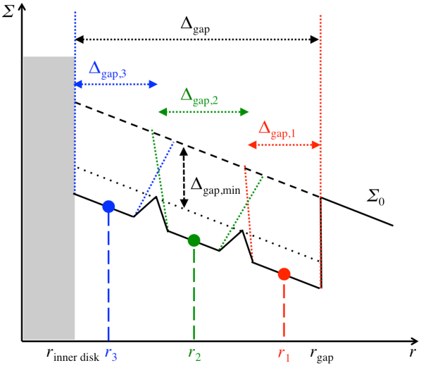
Figure 1.— Illustration of a common gap opened by 3 planets located at $r_{1}$, $r_{2}$, and $r_{3}$. $\Sigma_{0}$ (and its dashed line extension in the gap) indicates the original undepleted gas surface density. $\Delta_{\rm gap,1}$, $\Delta_{\rm gap,2}$, and $\Delta_{\rm gap,3}$ are the widths of the individual gaps opened by each planet if it were alone in the disk. $\delta_{\rm gap,min}$ is the minimum depletion factor inside the gap, which in the illustration is only reached at the joint edges of individual gaps, whereas most of the gap has a larger depletion factor. The shaded region marks the poorly constrained inner disk. See Section 2 for details.

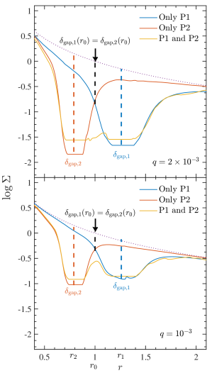
Figure 2.— The profiles of the individual gaps opened by a planet at $r_{\rm 1}$ (blue curves) or $r_{\rm 2}$ (red curves), and the profile of the common gap opened by both planets (yellow curves). Upper panel: individual gaps opened by two $q=2\times 10^{-3}$ planets just merge to form a (complete) common gap ($\delta_{\rm gap,1}(r_{0})=\delta_{\rm gap,2}(r_{0})\approx\sqrt{\delta_{\rm gap,1}}\approx\sqrt{\delta_{\rm gap,2}}$; $r_{0}\approx 1$). Bottom: two less massive planets with $q=10^{-3}$ at the same locations are unable to open a complete common gap ($\delta_{\rm gap,1}(r_{0})=\delta_{\rm gap,2}(r_{0})<\sqrt{\delta_{\rm gap,1}}\approx\sqrt{\delta_{\rm gap,2}}$). The black dotted line is the initial surface density profile (i.e., $\Sigma_{0}(r)$). The colored text boxes on the curves indicate the depletion factors of various gaps at certain locations, illustrated by the vertical dash lines of the same color.

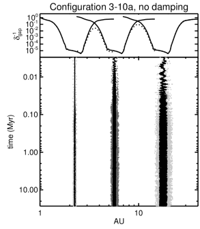
Figure 3.— The orbital evolution of system 3-10a in Table 2 without gas damping forces. The system is stable for at least 27 Myr. The top panel shows the depletion caused by planets’ gaps. The solid curves indicate individual gaps opened by each planet, while the dotted curve is the profile of the common gap calculated based on Equation 3. The bottom panel shows the temporal evolution of the semi-major axis $a$ (black) and periapse and apoapse (gray) of each planet.

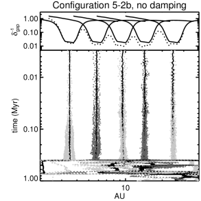
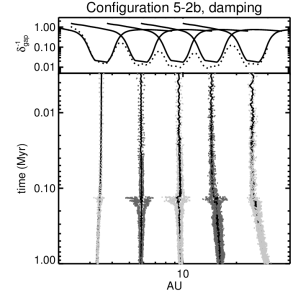
Figure 4.— The same as Figure 3, but for system 5-2b in Table 2, showing the cases when gas damping forces are not included (left; unstable) and included (right; stable). The gas gap density normalization on the right is $\Sigma_{30}=0.1$ g cm^-2.

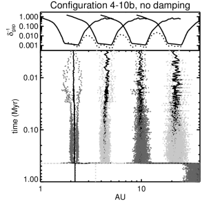
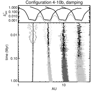
Figure 5.— The same as Figure 4, but for system 4-10b in Table 2. The gas gap density normalization on the right is $\Sigma_{30}=0.01$ g cm^-2.

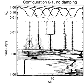
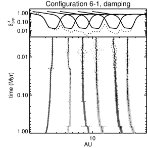
Figure 6.— The same as Figure 4, but for system 6-1 in Table 2. The gas gap density normalization on the right is $\Sigma_{30}=1$ g cm^-2.

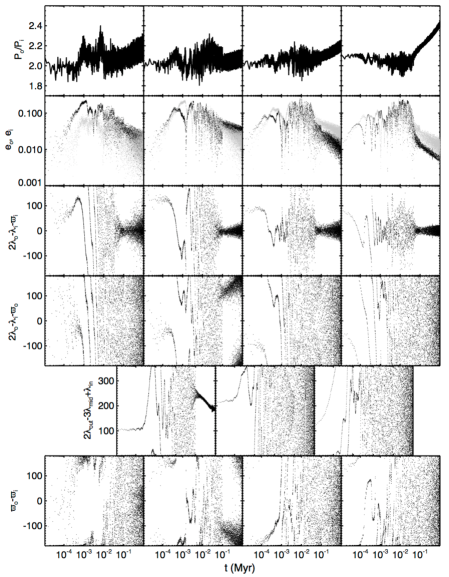
Figure 7.— Evolution of orbital elements for System 5-2b with gas damping included ($\Sigma_{30}=0.1$ g cm^-2; right panel in Figure 4). Row 1: period ratio of each adjacent pair of planets, from outer to inner. Row 2: eccentricity of outer planet (gray) and inner planet (black). Row 3: 2:1 mean motion resonant argument involving the longitude of periapse of the inner planet. Row 4: 2:1 mean motion resonant argument involving the longitude of periapse of the outer planet. Row 5: Three-body resonant argument (Laplace resonance). Row 6: Separation of adjacent planets’ longitude of periapses.

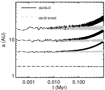
Figure 8.— The application of an $\dot{a}$ fine-tuned to each planet (gray) can counteract the effects of resonant repulsion (black,$\dot{a}$). The example shown is for Configuration 4-10a.

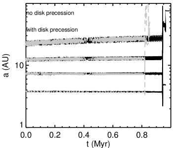
Figure 9.— Precession caused by an outer disk (approximately as a 10 Jupiter mass ring at 50 AU) does not significantly change the stability timescale. The example shown is for Configuration 4-10d with $\Sigma_{30}=0.01$g cm^-2.

Figure 10.— Probability contour of initial resonant fraction vs. disruption timescale (Eqn. B1 and B2) to account for the stellar ages and absence or presence of 2:1 commensurabilities in the Koriski & Zucker (2011) collection. The contours are for $[.01,.05,.2,.5,.9]$, normalized to the highest probability. The dashed line represents the present day 5/30 fraction of 2:1 commensurabilities in the collection.

Figure 11.— Probability contour of initial resonant fraction vs. maximum disruption timescale (Eqn. B1 and B3; the maximum disruption timescale is an upper cut-off for a log uniform distribution of disruption timescales) to account for the stellar ages and absence or presence of 2:1 commensurabilities in the Koriski & Zucker (2011) collection. The contours are for $[.01,.05,.2,.5,.9]$, normalized to the highest probability. The dashed line represents the present day 5/30 fraction of 2:1 commensurabilities in the collection.

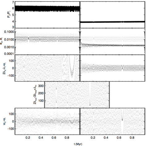
Figure 12.— Evolution of orbital elements for System 3-5 with gas damping included (Table 2; $\Sigma_{30}=0.01$ g cm^-2). Row 1: period ratio of each adjacent pair of planets, from outer to inner. Row 2: eccentricity of outer planet (gray) and inner planet (black). Row 3: 2:1 mean motion resonant argument involving the longitude of periapse of the inner planet. Row 4: Three-body resonant argument (Laplace resonance). Row 5: Separation of adjacent planets’ longitude of periapses.

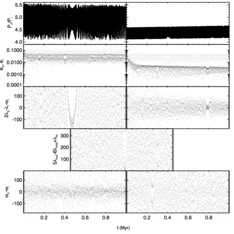
Figure 13.— Evolution of orbital elements for System 3-10a with gas damping included (Table 2; $\Sigma_{30}=0.001$ g cm^-2). Row 1: period ratio of each adjacent pair of planets, from outer to inner. Row 2: eccentricity of outer planet (gray) and inner planet (black). Row 3: 2:1 mean motion resonant argument involving the longitude of periapse of the inner planet. Row 4: Three-body resonant argument. Row 5: Separation of adjacent planets’ longitude of periapses.

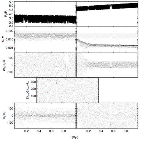
Figure 14.— Evolution of orbital elements for System 3-10b with gas damping included (Table 2; $\Sigma_{30}=0.01$ g cm^-2). Row 1: period ratio of each adjacent pair of planets, from outer to inner. Row 2: eccentricity of outer planet (gray) and inner planet (black). Row 3: 2:1 mean motion resonant argument involving the longitude of periapse of the inner planet. Row 4: Three-body resonant argument (Laplace resonance). Row 5: Separation of adjacent planets’ longitude of periapses.

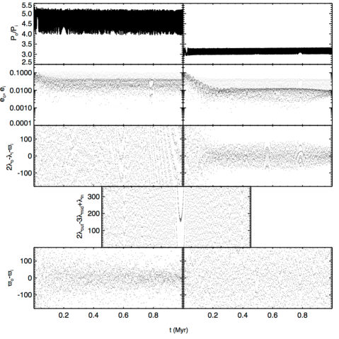
Figure 15.— Evolution of orbital elements for System 3-10c with gas damping included (Table 2; $\Sigma_{30}=0.001$ g cm^-2). Row 1: period ratio of each adjacent pair of planets, from outer to inner. Row 2: eccentricity of outer planet (gray) and inner planet (black). Row 3: 2:1 mean motion resonant argument involving the longitude of periapse of the inner planet. Row 4: Three-body resonant argument (Laplace resonance). Row 5: Separation of adjacent planets’ longitude of periapses.

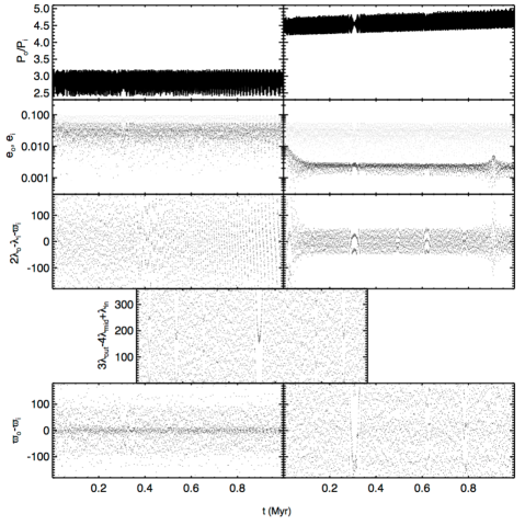
Figure 16.— Evolution of orbital elements for System 3-10d with gas damping included (Table 2; $\Sigma_{30}=0.01$ g cm^-2). Row 1: period ratio of each adjacent pair of planets, from outer to inner. Row 2: eccentricity of outer planet (gray) and inner planet (black). Row 3: 2:1 mean motion resonant argument involving the longitude of periapse of the inner planet.Row 4: Three-body resonant argument. Row 5: Separation of adjacent planets’ longitude of periapses.

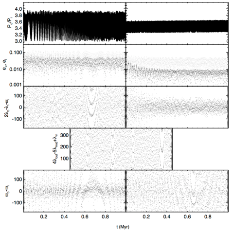
Figure 17.— Evolution of orbital elements for System 3-10e with gas damping included (Table 2; $\Sigma_{30}=0.1$ g cm^-2). Row 1: period ratio of each adjacent pair of planets, from outer to inner. Row 2: eccentricity of outer planet (gray) and inner planet (black). Row 3: 2:1 mean motion resonant argument involving the longitude of periapse of the inner planet. Row 4: Three-body resonant argument. Row 5: Separation of adjacent planets’ longitude of periapses.

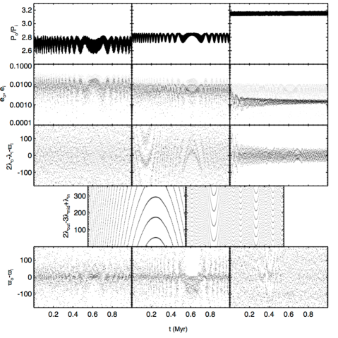
Figure 18.— Evolution of orbital elements for System 4-2 with gas damping included (Table 2; $\Sigma_{30}=0.01$ g cm^-2). Row 1: period ratio of each adjacent pair of planets, from outer to inner. Row 2: eccentricity of outer planet (gray) and inner planet (black). Row 3: 2:1 mean motion resonant argument involving the longitude of periapse of the inner planet. Row 4: Three-body resonant argument (Laplace resonance). Row 5: Separation of adjacent planets’ longitude of periapses.

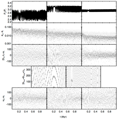
Figure 19.— Evolution of orbital elements for System 4-5a with gas damping included (Table 2; $\Sigma_{30}=0.001$ g cm^-2). Row 1: period ratio of each adjacent pair of planets, from outer to inner. Row 2: eccentricity of outer planet (gray) and inner planet (black). Row 3: 2:1 mean motion resonant argument involving the longitude of periapse of the inner planet. Row 4: Three-body resonant argument. Row 5: Separation of adjacent planets’ longitude of periapses.

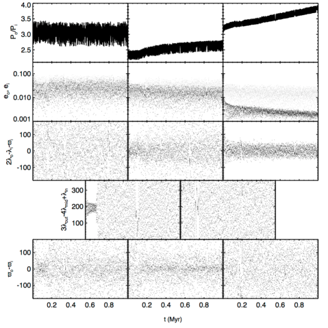
Figure 20.— Evolution of orbital elements for System 4-5b with gas damping included (Table 2; $\Sigma_{30}=0.01$ g cm^-2). Row 1: period ratio of each adjacent pair of planets, from outer to inner. Row 2: eccentricity of outer planet (gray) and inner planet (black). Row 3: 2:1 mean motion resonant argument involving the longitude of periapse of the inner planet. Row 4: Three-body resonant argument. Row 5: Separation of adjacent planets’ longitude of periapses.

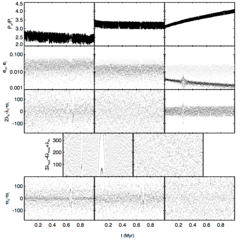
Figure 21.— Evolution of orbital elements for System 4-5c with gas damping included (Table 2; $\Sigma_{30}=0.1$ g cm^-2). Row 1: period ratio of each adjacent pair of planets, from outer to inner. Row 2: eccentricity of outer planet (gray) and inner planet (black). Row 3: 2:1 mean motion resonant argument involving the longitude of periapse of the inner planet. Row 4: Three-body resonant argument. Row 5: Separation of adjacent planets’ longitude of periapses.

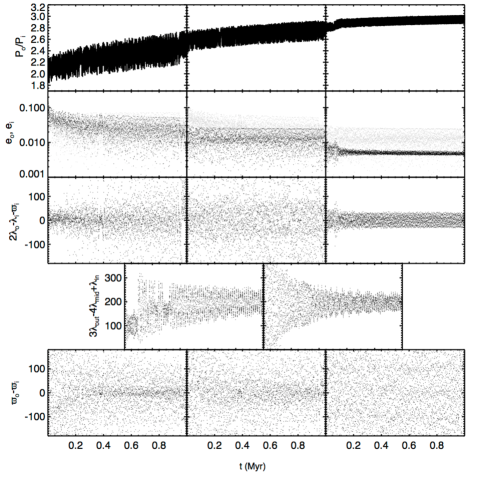
Figure 22.— Evolution of orbital elements for System 4-5d with gas damping included (Table 2; $\Sigma_{30}=0.1$ g cm^-2). Row 1: period ratio of each adjacent pair of planets, from outer to inner. Row 2: eccentricity of outer planet (gray) and inner planet (black). Row 3: 2:1 mean motion resonant argument involving the longitude of periapse of the inner planet. Row 4: Three-body resonant argument. Row 5: Separation of adjacent planets’ longitude of periapses.

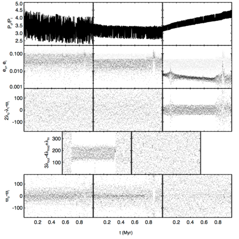
Figure 23.— Evolution of orbital elements for System 4-10a with gas damping included (Table 2; $\Sigma_{30}=0.01$ g cm^-2). Row 1: period ratio of each adjacent pair of planets, from outer to inner. Row 2: eccentricity of outer planet (gray) and inner planet (black). Row 3: 2:1 mean motion resonant argument involving the longitude of periapse of the inner planet. Row 4: Three-body resonant argument. Row 5: Separation of adjacent planets’ longitude of periapses.

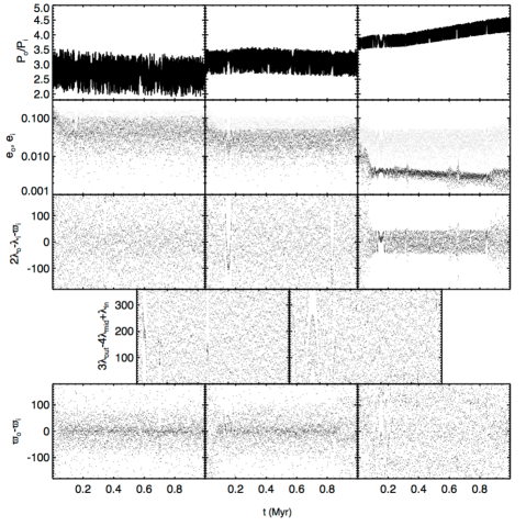
Figure 24.— Evolution of orbital elements for System 4-10b with gas damping included (Table 2; $\Sigma_{30}=0.01$ g cm^-2). Row 1: period ratio of each adjacent pair of planets, from outer to inner. Row 2: eccentricity of outer planet (gray) and inner planet (black). Row 3: 2:1 mean motion resonant argument involving the longitude of periapse of the inner planet. Row 4: Three-body resonant argument. Row 5: Separation of adjacent planets’ longitude of periapses.

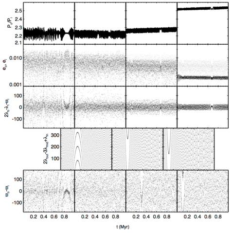
Figure 25.— Evolution of orbital elements for System 5-1 with gas damping included (Table 2; $\Sigma_{30}=0.1$ g cm^-2). Row 1: period ratio of each adjacent pair of planets, from outer to inner. Row 2: eccentricity of outer planet (gray) and inner planet (black). Row 3: 2:1 mean motion resonant argument involving the longitude of periapse of the inner planet. Row 4: Three-body resonant argument (Laplace resonance). Row 5: Separation of adjacent planets’ longitude of periapses.

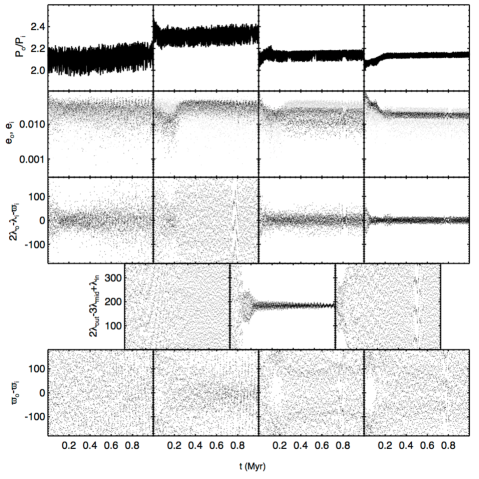
Figure 26.— Evolution of orbital elements for System 5-2a with gas damping included (Table 2; $\Sigma_{30}=0.01$ g cm^-2). Row 1: period ratio of each adjacent pair of planets, from outer to inner. Row 2: eccentricity of outer planet (gray) and inner planet (black). Row 3: 2:1 mean motion resonant argument involving the longitude of periapse of the inner planet. Row 4: Three-body resonant argument (Laplace resonance). Row 5: Separation of adjacent planets’ longitude of periapses.

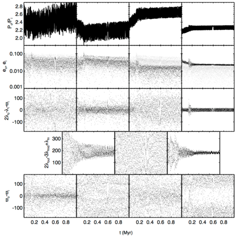
Figure 27.— Evolution of orbital elements for System 5-5a with gas damping included (Table 2; $\Sigma_{30}=0.01$ g cm^-2). Row 1: period ratio of each adjacent pair of planets, from outer to inner. Row 2: eccentricity of outer planet (gray) and inner planet (black). Row 3: 2:1 mean motion resonant argument involving the longitude of periapse of the inner planet. Row 4: Three-body resonant argument (Laplace resonance). Row 5: Separation of adjacent planets’ longitude of periapses.

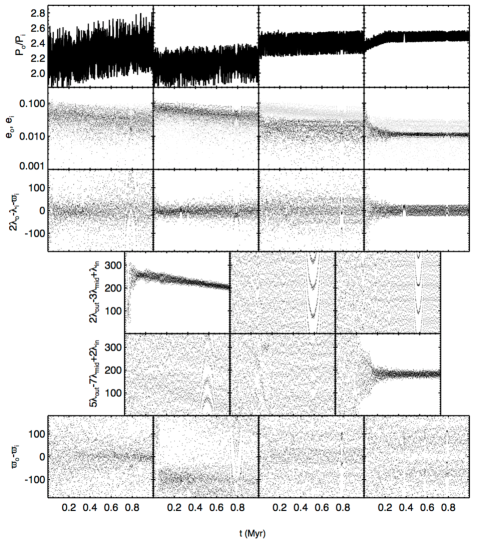
Figure 28.— Evolution of orbital elements for System 5-5b with gas damping included (Table 2; $\Sigma_{30}=0.01$ g cm^-2). Row 1: period ratio of each adjacent pair of planets, from outer to inner. Row 2: eccentricity of outer planet (gray) and inner planet (black). Row 3: 2:1 mean motion resonant argument involving the longitude of periapse of the inner planet. Row 4: Three-body resonant argument (Laplace resonance). Row 5: Separation of adjacent planets’ longitude of periapses.

Figure 29.— Evolution of orbital elements for System 5-5c with gas damping included (Table 2; $\Sigma_{30}=0.01$ g cm^-2). Row 1: period ratio of each adjacent pair of planets, from outer to inner. Row 2: eccentricity of outer planet (gray) and inner planet (black). Row 3: 2:1 mean motion resonant argument involving the longitude of periapse of the inner planet. Row 4: Three-body resonant argument (Laplace resonance). Row 5: Separation of adjacent planets’ longitude of periapses.

Figure 30.— Evolution of orbital elements for System 6-0.5 with gas damping included (Table 2; $\Sigma_{30}=1$ g cm^-2). Row 1: period ratio of each adjacent pair of planets, from outer to inner. Row 2: eccentricity of outer planet (gray) and inner planet (black). Row 3: 2:1 mean motion resonant argument involving the longitude of periapse of the inner planet. Row 4: 3:2 mean motion resonant argument involving the longitude of periapse of the inner planet. Row 5: Three-body resonant argument. Row 6: Separation of adjacent planets’ longitude of periapses.

Figure 31.— Evolution of orbital elements for System 6-1 with gas damping included (Table 2; $\Sigma_{30}=1$ g cm^-2). Row 1: period ratio of each adjacent pair of planets, from outer to inner. Row 2: eccentricity of outer planet (gray) and inner planet (black). Row 3: 2:1 mean motion resonant argument involving the longitude of periapse of the inner planet. Row 4: 3:2 mean motion resonant argument involving the longitude of periapse of the inner planet. Row 5: Three-body resonant argument. Row 6: Separation of adjacent planets’ longitude of periapses.

References

- Alexander et al. (2014) Alexander, R., Pascucci, I., Andrews, S., Armitage, P., & Cieza, L. 2014, Protostars and Planets VI, 475
- Alexander et al. (2006) Alexander, R. D., Clarke, C. J., & Pringle, J. E. 2006, MNRAS, 369, 229
- ALMA Partnership et al. (2015) ALMA Partnership, et al. 2015, ApJ, 808, L3
- Andrews et al. (2013) Andrews, S. M., Rosenfeld, K. A., Kraus, A. L., & Wilner, D. J. 2013, ApJ, 771, 129
- Andrews et al. (2011) Andrews, S. M., Wilner, D. J., Espaillat, C., Hughes, A. M., Dullemond, C. P., McClure, M. K., Qi, C., & Brown, J. M. 2011, ApJ, 732, 42
- Avenhaus et al. (2014) Avenhaus, H., Quanz, S. P., Schmid, H. M., Meyer, M. R., Garufi, A., Wolf, S., & Dominik, C. 2014, ApJ, 781, 87
- Bai (2011a) Bai, X.-N. 2011a, ApJ, 739, 50
- Bai (2011b) —. 2011b, ApJ, 739, 51
- Bai (2015) —. 2015, ApJ, 798, 84
- Bai & Stone (2011) Bai, X.-N., & Stone, J. M. 2011, ApJ, 736, 144
- Beaugé & Nesvorný (2012) Beaugé, C., & Nesvorný, D. 2012, ApJ, 751, 119
- Beuzit et al. (2008) Beuzit, J.-L., et al. 2008, in Society of Photo-Optical Instrumentation Engineers (SPIE) Conference Series, Vol. 7014, Society of Photo-Optical Instrumentation Engineers (SPIE) Conference Series
- Biller et al. (2012) Biller, B., et al. 2012, ApJ, 753, L38
- Birnstiel et al. (2012) Birnstiel, T., Andrews, S. M., & Ercolano, B. 2012, A&A, 544, A79
- Boss (1998) Boss, A. P. 1998, ApJ, 503, 923
- Bowler et al. (2010) Bowler, B. P., et al. 2010, ApJ, 709, 396
- Brandt et al. (2014) Brandt, T. D., et al. 2014, ApJ, 794, 159
- Briceño et al. (2002) Briceño, C., Luhman, K. L., Hartmann, L., Stauffer, J. R., & Kirkpatrick, J. D. 2002, ApJ, 580, 317
- Brittain et al. (2014) Brittain, S. D., Carr, J. S., Najita, J. R., Quanz, S. P., & Meyer, M. R. 2014, ApJ, 791, 136
- Bruderer et al. (2014) Bruderer, S., van der Marel, N., van Dishoeck, E. F., & van Kempen, T. A. 2014, A&A, 562, A26
- Bryan et al. (2016) Bryan, M. L., et al. 2016, ArXiv e-prints
- Calvet et al. (2002) Calvet, N., D’Alessio, P., Hartmann, L., Wilner, D., Walsh, A., & Sitko, M. 2002, ApJ, 568, 1008
- Canovas et al. (2013) Canovas, H., Ménard, F., Hales, A., Jordán, A., Schreiber, M. R., Casassus, S., Gledhill, T. M., & Pinte, C. 2013, A&A, 556, A123
- Casassus et al. (2013) Casassus, S., et al. 2013, Nature, 493, 191
- Chambers et al. (1996) Chambers, J. E., Wetherill, G. W., & Boss, A. P. 1996, Icarus, 119, 261
- Chatterjee et al. (2008) Chatterjee, S., Ford, E. B., Matsumura, S., & Rasio, F. A. 2008, ApJ, 686, 580
- Chiang & Murray-Clay (2007) Chiang, E., & Murray-Clay, R. 2007, Nature Physics, 3, 604
- Cieza et al. (2012) Cieza, L. A., Schreiber, M. R., Romero, G. A., Williams, J. P., Rebassa-Mansergas, A., & Merín, B. 2012, ApJ, 750, 157
- Clarke et al. (2001) Clarke, C. J., Gendrin, A., & Sotomayor, M. 2001, MNRAS, 328, 485
- Close et al. (2014) Close, L. M., et al. 2014, ApJ, 781, L30
- Crida et al. (2009) Crida, A., Masset, F., & Morbidelli, A. 2009, ApJ, 705, L148
- Crida et al. (2006) Crida, A., Morbidelli, A., & Masset, F. 2006, Icarus, 181, 587
- Cumming et al. (2008) Cumming, A., Butler, R. P., Marcy, G. W., Vogt, S. S., Wright, J. T., & Fischer, D. A. 2008, PASP, 120, 531
- Dawson et al. (2015a) Dawson, R. I., Chiang, E., & Lee, E. J. 2015a, ArXiv:1506.06867
- Dawson et al. (2015b) Dawson, R. I., Lee, E. J., & Chiang, E. 2015b, ArXiv e-prints
- Dawson & Murray-Clay (2013) Dawson, R. I., & Murray-Clay, R. A. 2013, ApJ, 767, L24
- de Juan Ovelar et al. (2013) de Juan Ovelar, M., Min, M., Dominik, C., Thalmann, C., Pinilla, P., Benisty, M., & Birnstiel, T. 2013, A&A, 560, A111
- Dipierro et al. (2015) Dipierro, G., Price, D., Laibe, G., Hirsh, K., Cerioli, A., & Lodato, G. 2015, MNRAS, 453, L73
- Dodson-Robinson & Salyk (2011) Dodson-Robinson, S. E., & Salyk, C. 2011, ApJ, 738, 131
- Dodson-Robinson et al. (2009) Dodson-Robinson, S. E., Veras, D., Ford, E. B., & Beichman, C. A. 2009, ApJ, 707, 79
- Dong et al. (2012a) Dong, R., et al. 2012a, ApJ, 760, 111
- Dong et al. (2012b) —. 2012b, ApJ, 750, 161
- Dong et al. (2011a) Dong, R., Rafikov, R. R., & Stone, J. M. 2011a, ApJ, 741, 57
- Dong et al. (2011b) Dong, R., Rafikov, R. R., Stone, J. M., & Petrovich, C. 2011b, ApJ, 741, 56
- Dong et al. (2015a) Dong, R., Zhu, Z., Rafikov, R. R., & Stone, J. M. 2015a, ApJ, 809, L5
- Dong et al. (2015b) Dong, R., Zhu, Z., & Whitney, B. 2015b, ApJ, 809, 93
- Downes et al. (2015) Downes, J. J., et al. 2015, MNRAS, 450, 3490
- Duffell (2015) Duffell, P. C. 2015, ApJ, 807, L11
- Duffell & Chiang (2015) Duffell, P. C., & Chiang, E. 2015, ApJ, 812, 94
- Duffell & Dong (2015) Duffell, P. C., & Dong, R. 2015, ApJ, 802, 42
- Duffell et al. (2014) Duffell, P. C., Haiman, Z., MacFadyen, A. I., D’Orazio, D. J., & Farris, B. D. 2014, ApJ, 792, L10
- Duffell & MacFadyen (2013) Duffell, P. C., & MacFadyen, A. I. 2013, ApJ, 769, 41
- Dullemond & Dominik (2005) Dullemond, C. P., & Dominik, C. 2005, A&A, 434, 971
- Dunhill et al. (2013) Dunhill, A. C., Alexander, R. D., & Armitage, P. J. 2013, MNRAS, 428, 3072
- Dürmann & Kley (2015) Dürmann, C., & Kley, W. 2015, A&A, 574, A52
- Espaillat et al. (2007) Espaillat, C., Calvet, N., D’Alessio, P., Hernández, J., Qi, C., Hartmann, L., Furlan, E., & Watson, D. M. 2007, ApJ, 670, L135
- Espaillat et al. (2014) Espaillat, C., et al. 2014, ArXiv e-prints
- Fabrycky & Murray-Clay (2010) Fabrycky, D. C., & Murray-Clay, R. A. 2010, ApJ, 710, 1408
- Flaherty et al. (2015) Flaherty, K. M., Hughes, A. M., Rosenfeld, K. A., Andrews, S. M., Chiang, E., Simon, J. B., Kerzner, S., & Wilner, D. J. 2015, ApJ, 813, 99
- Ford & Chiang (2007) Ford, E. B., & Chiang, E. I. 2007, ApJ, 661, 602
- Fouchet et al. (2010) Fouchet, L., Gonzalez, J.-F., & Maddison, S. T. 2010, A&A, 518, A16
- Fukagawa et al. (2013) Fukagawa, M., et al. 2013, PASJ, 65, L14
- Fung (2015) Fung, J. 2015, PhD thesis, University of Toronto, Canada
- Fung et al. (2014) Fung, J., Shi, J.-M., & Chiang, E. 2014, ApJ, 782, 88
- Gammie (1996) Gammie, C. F. 1996, ApJ, 457, 355
- Garufi et al. (2013) Garufi, A., et al. 2013, A&A, 560, A105
- Goldreich et al. (2004) Goldreich, P., Lithwick, Y., & Sari, R. 2004, ARA&A, 42, 549
- Gonzalez et al. (2012) Gonzalez, J.-F., Pinte, C., Maddison, S. T., Ménard, F., & Fouchet, L. 2012, A&A, 547, A58
- Goodman & Rafikov (2001) Goodman, J., & Rafikov, R. R. 2001, ApJ, 552, 793
- Grady et al. (2013) Grady, C. A., et al. 2013, ApJ, 762, 48
- Hartmann et al. (1998) Hartmann, L., Calvet, N., Gullbring, E., & D’Alessio, P. 1998, ApJ, 495, 385
- Hashimoto et al. (2012) Hashimoto, J., et al. 2012, ApJ, 758, L19
- Hashimoto et al. (2015) —. 2015, ApJ, 799, 43
- Heng & Kenyon (2010) Heng, K., & Kenyon, S. J. 2010, MNRAS, 408, 1476
- Howard et al. (2012) Howard, A. W., et al. 2012, ApJS, 201, 15
- Howard et al. (2010) —. 2010, Science, 330, 653
- Huélamo et al. (2011) Huélamo, N., Lacour, S., Tuthill, P., Ireland, M., Kraus, A., & Chauvin, G. 2011, A&A, 528, L7
- Isella et al. (2013) Isella, A., Pérez, L. M., Carpenter, J. M., Ricci, L., Andrews, S., & Rosenfeld, K. 2013, ApJ, 775, 30
- Johnson et al. (2010) Johnson, J. A., Aller, K. M., Howard, A. W., & Crepp, J. R. 2010, PASP, 122, 905
- Jones et al. (2003) Jones, H. R. A., Butler, R. P., Tinney, C. G., Marcy, G. W., Penny, A. J., McCarthy, C., & Carter, B. D. 2003, MNRAS, 341, 948
- Juhász et al. (2015) Juhász, A., Benisty, M., Pohl, A., Dullemond, C. P., Dominik, C., & Paardekooper, S.-J. 2015, MNRAS, 451, 1147
- Jurić & Tremaine (2008) Jurić, M., & Tremaine, S. 2008, ApJ, 686, 603
- Kanagawa et al. (2015) Kanagawa, K. D., Muto, T., Tanaka, H., Tanigawa, T., Takeuchi, T., Tsukagoshi, T., & Momose, M. 2015, ApJ, 806, L15
- Koepferl et al. (2013) Koepferl, C. M., Ercolano, B., Dale, J., Teixeira, P. S., Ratzka, T., & Spezzi, L. 2013, MNRAS, 428, 3327
- Kominami & Ida (2002) Kominami, J., & Ida, S. 2002, Icarus, 157, 43
- Koriski & Zucker (2011) Koriski, S., & Zucker, S. 2011, ApJ, 741, L23
- Kratter et al. (2010) Kratter, K. M., Murray-Clay, R. A., & Youdin, A. N. 2010, ApJ, 710, 1375
- Kraus & Ireland (2012) Kraus, A. L., & Ireland, M. J. 2012, ApJ, 745, 5
- Kraus et al. (2011) Kraus, A. L., Ireland, M. J., Martinache, F., & Hillenbrand, L. A. 2011, ApJ, 731, 8
- Kuzuhara et al. (2013) Kuzuhara, M., et al. 2013, ApJ, 774, 11
- Lada et al. (2006) Lada, C. J., et al. 2006, AJ, 131, 1574
- Lagrange et al. (2010) Lagrange, A.-M., et al. 2010, Science, 329, 57
- Li et al. (2000) Li, H., Finn, J. M., Lovelace, R. V. E., & Colgate, S. A. 2000, ApJ, 533, 1023
- Li et al. (2009) Li, H., Lubow, S. H., Li, S., & Lin, D. N. C. 2009, ApJ, 690, L52
- Lin (2012) Lin, M.-K. 2012, MNRAS, 426, 3211
- Lin & Papaloizou (2010) Lin, M.-K., & Papaloizou, J. C. B. 2010, MNRAS, 405, 1473
- Lithwick & Wu (2012) Lithwick, Y., & Wu, Y. 2012, ApJ, 756, L11
- Luhman et al. (2010) Luhman, K. L., Allen, P. R., Espaillat, C., Hartmann, L., & Calvet, N. 2010, ApJS, 186, 111
- Lyra et al. (2009) Lyra, W., Johansen, A., Klahr, H., & Piskunov, N. 2009, A&A, 493, 1125
- Lyra & Lin (2013) Lyra, W., & Lin, M.-K. 2013, ApJ, 775, 17
- Macintosh et al. (2015) Macintosh, B., et al. 2015, ArXiv e-prints
- Macintosh et al. (2008) Macintosh, B. A., et al. 2008, in Society of Photo-Optical Instrumentation Engineers (SPIE) Conference Series, Vol. 7015, Society of Photo-Optical Instrumentation Engineers (SPIE) Conference Series
- Marois et al. (2008) Marois, C., Macintosh, B., Barman, T., Zuckerman, B., Song, I., Patience, J., Lafrenière, D., & Doyon, R. 2008, Science, 322, 1348
- Marois et al. (2010) Marois, C., Zuckerman, B., Konopacky, Q. M., Macintosh, B., & Barman, T. 2010, Nature, 468, 1080
- Mayama et al. (2012) Mayama, S., et al. 2012, ApJ, 760, L26
- Mayor et al. (2011) Mayor, M., et al. 2011, ArXiv e-prints
- Michtchenko & Malhotra (2004) Michtchenko, T. A., & Malhotra, R. 2004, Icarus, 168, 237
- Mittal & Chiang (2015) Mittal, T., & Chiang, E. 2015, ApJ, 798, L25
- Montet et al. (2014) Montet, B. T., Crepp, J. R., Johnson, J. A., Howard, A. W., & Marcy, G. W. 2014, ApJ, 781, 28
- Moore & Quillen (2013) Moore, A., & Quillen, A. C. 2013, MNRAS, 430, 320
- Morbidelli et al. (2007) Morbidelli, A., Tsiganis, K., Crida, A., Levison, H. F., & Gomes, R. 2007, AJ, 134, 1790
- Muto et al. (2012) Muto, T., et al. 2012, ApJ, 748, L22
- Muto et al. (2010) Muto, T., Suzuki, T. K., & Inutsuka, S.-i. 2010, ApJ, 724, 448
- Muzerolle et al. (2010) Muzerolle, J., Allen, L. E., Megeath, S. T., Hernández, J., & Gutermuth, R. A. 2010, ApJ, 708, 1107
- Nagasawa & Ida (2011) Nagasawa, M., & Ida, S. 2011, ApJ, 742, 72
- Najita et al. (2015) Najita, J. R., Andrews, S. M., & Muzerolle, J. 2015, MNRAS, 450, 3559
- Owen & Clarke (2012) Owen, J. E., & Clarke, C. J. 2012, MNRAS, 426, L96
- Owen et al. (2012) Owen, J. E., Clarke, C. J., & Ercolano, B. 2012, MNRAS, 422, 1880
- Papaloizou & Larwood (2000) Papaloizou, J. C. B., & Larwood, J. D. 2000, MNRAS, 315, 823
- Pérez et al. (2014) Pérez, L. M., Isella, A., Carpenter, J. M., & Chandler, C. J. 2014, ApJ, 783, L13
- Perez et al. (2015) Perez, S., Casassus, S., Ménard, F., et al. 2015, ApJ, 798, 85
- Perez-Becker & Chiang (2011a) Perez-Becker, D., & Chiang, E. 2011a, ApJ, 735, 8
- Perez-Becker & Chiang (2011b) —. 2011b, ApJ, 727, 2
- Pinilla et al. (2012) Pinilla, P., Benisty, M., & Birnstiel, T. 2012, A&A, 545, A81
- Pohl et al. (2015) Pohl, A., Pinilla, P., Benisty, M., Ataiee, S., Juhász, A., Dullemond, C. P., Van Boekel, R., & Henning, T. 2015, MNRAS, 453, 1768
- Pollack et al. (1996) Pollack, J. B., Hubickyj, O., Bodenheimer, P., Lissauer, J. J., Podolak, M., & Greenzweig, Y. 1996, Icarus, 124, 62
- Pontoppidan et al. (2008) Pontoppidan, K. M., Blake, G. A., van Dishoeck, E. F., Smette, A., Ireland, M. J., & Brown, J. 2008, ApJ, 684, 1323
- Pott et al. (2010) Pott, J.-U., Perrin, M. D., Furlan, E., Ghez, A. M., Herbst, T. M., & Metchev, S. 2010, ApJ, 710, 265
- Quanz et al. (2013) Quanz, S. P., Amara, A., Meyer, M. R., Kenworthy, M. A., Kasper, M., & Girard, J. H. 2013, ApJ, 766, L1
- Rafikov (2002) Rafikov, R. R. 2002, ApJ, 569, 997
- Rafikov (2005) —. 2005, ApJ, 621, L69
- Rameau et al. (2013) Rameau, J., et al. 2013, ApJ, 772, L15
- Rasio & Ford (1996) Rasio, F. A., & Ford, E. B. 1996, Science, 274, 954
- Reggiani et al. (2014) Reggiani, M., et al. 2014, ApJ, 792, L23
- Rein (2012) Rein, H. 2012, MNRAS, 422, 3611
- Rice et al. (2015) Rice, K., Lopez, E., Forgan, D., & Biller, B. 2015, ArXiv e-prints
- Rosotti et al. (2013) Rosotti, G. P., Ercolano, B., Owen, J. E., & Armitage, P. J. 2013, MNRAS, 430, 1392
- Sallum et al. (2015) Sallum, S., et al. 2015, Nature, 527, 342
- Salyk et al. (2009) Salyk, C., Blake, G. A., Boogert, A. C. A., & Brown, J. M. 2009, ApJ, 699, 330
- Shakura & Sunyaev (1973) Shakura, N. I., & Sunyaev, R. A. 1973, A&A, 24, 337
- Shvartzvald et al. (2016) Shvartzvald, Y., et al. 2016, MNRAS, 457, 4089
- Simon et al. (2013) Simon, J. B., Bai, X.-N., Stone, J. M., Armitage, P. J., & Beckwith, K. 2013, ApJ, 764, 66
- Skrutskie et al. (1990) Skrutskie, M. F., Dutkevitch, D., Strom, S. E., Edwards, S., Strom, K. M., & Shure, M. A. 1990, AJ, 99, 1187
- Smith & Lissauer (2009a) Smith, A. W., & Lissauer, J. J. 2009a, Icarus, 201, 381
- Smith & Lissauer (2009b) —. 2009b, Icarus, 201, 381
- Snellgrove et al. (2001) Snellgrove, M. D., Papaloizou, J. C. B., & Nelson, R. P. 2001, A&A, 374, 1092
- Strom et al. (1989) Strom, K. M., Strom, S. E., Edwards, S., Cabrit, S., & Skrutskie, M. F. 1989, AJ, 97, 1451
- Tamayo et al. (2015) Tamayo, D., Triaud, A. H. M. J., Menou, K., & Rein, H. 2015, ArXiv e-prints
- Thommes et al. (2008) Thommes, E. W., Bryden, G., Wu, Y., & Rasio, F. A. 2008, ApJ, 675, 1538
- Tsang (2014) Tsang, D. 2014, ApJ, 782, 112
- Tsang et al. (2014) Tsang, D., Turner, N. J., & Cumming, A. 2014, ApJ, 782, 113
- Tsiganis et al. (2005) Tsiganis, K., Gomes, R., Morbidelli, A., & Levison, H. F. 2005, Nature, 435, 459
- Tsukagoshi et al. (2014) Tsukagoshi, T., et al. 2014, ApJ, 783, 90
- Turner et al. (2014) Turner, N. J., Fromang, S., Gammie, C., Klahr, H., Lesur, G., Wardle, M., & Bai, X.-N. 2014, Protostars and Planets VI, 411
- van der Marel et al. (2016) van der Marel, N., van Dishoeck, E. F., Bruderer, S., Andrews, S. M., Pontoppidan, K. M., Herczeg, G. J., van Kempen, T., & Miotello, A. 2016, A&A, 585, A58
- van der Marel et al. (2013) van der Marel, N., et al. 2013, Science, 340, 1199
- van der Marel et al. (2015) van der Marel, N., van Dishoeck, E. F., Bruderer, S., Pérez, L., & Isella, A. 2015, A&A, 579, A106
- van Dishoeck et al. (2015) van Dishoeck, E. F., van der Marel, N., Bruderer, S., & Pinilla, P. 2015, ArXiv e-prints
- Ward (1997) Ward, W. R. 1997, Icarus, 126, 261
- Wittenmyer et al. (2016) Wittenmyer, R. A., et al. 2016, ArXiv e-prints
- Wolff et al. (2012) Wolff, S., Dawson, R., & Murray-Clay, R. 2012, ApJ, 746, 171
- Yoshinaga et al. (1999) Yoshinaga, K., Kokubo, E., & Makino, J. 1999, Icarus, 139, 328
- Zhang et al. (2014) Zhang, K., Isella, A., Carpenter, J. M., & Blake, G. A. 2014, ApJ, 791, 42
- Zhou et al. (2007) Zhou, J.-L., Lin, D. N. C., & Sun, Y.-S. 2007, ApJ, 666, 423
- Zhu et al. (2012) Zhu, Z., Nelson, R. P., Dong, R., Espaillat, C., & Hartmann, L. 2012, ApJ, 755, 6
- Zhu et al. (2011) Zhu, Z., Nelson, R. P., Hartmann, L., Espaillat, C., & Calvet, N. 2011, ApJ, 729, 47
- Zhu & Stone (2014) Zhu, Z., & Stone, J. M. 2014, ApJ, 795, 53
- Zhu et al. (2013) Zhu, Z., Stone, J. M., & Rafikov, R. R. 2013, ApJ, 768, 143
- Zhu et al. (2014) Zhu, Z., Stone, J. M., Rafikov, R. R., & Bai, X.-n. 2014, ApJ, 785, 122