1 Introduction

Methods based on Markov chains play a critical role in statistical inference, where they form the basis of Markov chain Monte Carlo (MCMC) procedures for estimating intractable expectations [see, e.g., 9, 28]. In MCMC procedures, it is the stationary distribution of the Markov chain that typically encodes the information of interest. Thus, MCMC estimates are asymptotically exact, but their accuracy at finite times is limited by the convergence rate of the chain.

The usual measures of convergence rates of Markov chains—namely, the total variation mixing time or the absolute spectral gap of the transition matrix [21]—correspond to very strong notions of convergence and depend on global properties of the chain. Indeed, convergence of a Markov chain in total variation corresponds to uniform convergence of the expectations of all unit-bounded function to their equilibrium values. The resulting uniform bounds on the accuracy of expectations [4, 11, 18, 19, 20, 22, 27, 29] may be overly pessimistic—not indicative of the mixing times of specific expectations such as means and variances that are likely to be of interest in an inferential setting.

Another limitation of the uniform bounds is that they typically assume that the chain has arrived at the equilibrium distribution, at least approximately. Consequently, applying such bounds requires either assuming that the chain is started in equilibrium—impossible in practical applications of MCMC—or that the burn-in period is proportional to the mixing time of the chain, which is also unrealistic, if not impossible, in practical settings.

Given that the goal of MCMC is often to estimate specific expectations, as opposed to obtaining the stationary distribution, in the current paper we develop a function-specific notion of convergence with application to problems in Bayesian inference. We define a notion of “function-specific mixing time,” and we develop function-specific concentration bounds for Markov chains, as well as spectrum-based bounds on function-specific mixing times. We demonstrate the utility of both our overall framework and our particular concentration bounds by applying them to examples of MCMC-based data analysis from the literature and by using them to derive sharper confidence intervals and faster sequential testing procedures for MCMC.

1.1 Preliminaries

We focus on discrete time Markov chains on $d$ states given by a $d\times d$ transition matrix $P$ that satisfies the conditions of irreducibility, aperiodicity, and reversibility. These conditions guarantee the existence of a unique stationary distribution $\pi$. The issue is then to understand how quickly empirical averages of functions of the Markov chain, of the form $f:[d]\to[0,1]$, approach the stationary average, denoted by

$$\mu :\,=\mathbb{E}_{X\sim\pi}[f(X)].$$

The classical analysis of mixing defines convergence rate in terms of the total variation distance:

$$d_{\mathrm{TV}}\big{(}p,~{}q\big{)}=\sup_{f\colon\Omega\rightarrow[0,~{}1]}\Big{|}\mathbb{E}_{X\sim p}\big{[}f(X)\big{]}-\mathbb{E}_{Y\sim q}\big{[}f(Y)\big{]}\Big{|},$$ (1)

where the supremum ranges over all unit-bounded functions. The mixing time is then defined as the number of steps required to ensure that the chain is within total-variation distance $\delta$ of the stationary distribution—that is

$$T(\delta) :\,=\min\Big{\{}n\in\mathbb{N}\;\mid\;\max_{i\in[d]}d_{\mathrm{TV}}\big{(}\pi_{n}^{(i)},~{}\pi\big{)}\leq\delta\Big{\}},$$ (2)

where $\mathbb{N}=\{1,2,\ldots\}$ denotes the natural numbers, and $\pi_{n}^{(i)}$ is the distribution of the chain state $X_{n}$ given the starting state $X_{0}=i$.

Total variation is a worst-case measure of distance, and the resulting notion of mixing time can therefore be overly conservative when the Markov chain is being used to approximate the expectation of a fixed function, or expectations over some relatively limited class of functions. Accordingly, it is of interest to consider the following function-specific discrepancy measure:

Definition 1 ($f$-discrepancy).

For a given function $f$, the $f$-discrepancy is

$$d_{f}\big{(}p,~{}q\big{)}=\big{|}\mathbb{E}_{X\sim p}\big{[}f\big{(}X\big{)}\big{]}-\mathbb{E}_{Y\sim q}\big{[}f\big{(}Y\big{)}\big{]}\big{|}.$$ (3)

The $f$-discrepancy leads naturally to a function-specific notion of mixing time:

Definition 2 ($f$-mixing time).

For a given function $f$, the $f$-mixing time is

$$T_{f}\big{(}\delta\big{)}=\min\Big{\{}n\in\mathbb{N}\;\mid\;\max_{i\in[d]}d_{f}\big{(}\pi_{n}^{(i)},~{}\pi\big{)}\leq\delta\Big{\}}.$$ (4)

In the sequel, we also define function-specific notions of the spectral gap of a Markov chain, which can be used to bound the $f$-mixing time and to obtain function-specific concentration inequalities.

1.2 Related work

Mixing times are a classical topic of study in Markov chain theory, and there is a large collection of techniques for their analysis [see, e.g., 1, 6, 21, 23, 26, 30]. These tools and the results based on them, however, generally apply only to worst-case mixing times. Outside of specific examples [5, 7], relatively little is known about mixing with respect to individual functions or limited classes of functions. Similar limitations exist in studies of concentration of measure and studies of confidence intervals and other statistical functionals that depend on tail probability bounds. Existing bounds are generally uniform, or non-adaptive, and the rates that are reported include a factor that encodes the global mixing properties of the chain and does not adapt to the function [4, 11, 18, 19, 20, 22, 27, 29]. These factors, which do not appear in classic bounds for independent random variables, are generally either some variant of the spectral gap $\gamma$ of the transition matrix, or else a mixing time of the chain $T\big{(}\delta_{0}\big{)}$ for some absolute constant $\delta_{0}>0$. For example, the main theorem from [20] shows that for a function $f\colon[d]\rightarrow[0,~{}1]$ and a sample $X_{0}\sim\pi$ from the stationary distribution, we have

$$\mathbb{P}\big{(}\big{|}\frac{1}{N}\sum_{n=1}^{N}f\big{(}X_{n}\big{)}-\mu\big{|}\geq\epsilon\big{)}\leq 2\exp\Big{\{}-\frac{\gamma_{0}}{2\big{(}2-\gamma_{0}\big{)}}\cdot\epsilon^{2}N\Big{\}},$$ (5)

where the eigenvalues of $P$ are given in decreasing order as $1>\lambda_{2}(P)\geq\cdots\geq\lambda_{d}(P)$, and we denote the spectral gap of $P$ by

$$\gamma_{0}:\,=\min\big{\{}1-\lambda_{2}(P),~{}1\big{\}}.$$

The requirement that the chain start in equilibrium can be relaxed by adding a correction for the burn-in time [27]. Extensions of this and related bounds, including bounded-differences-type inequalities and generalizations to continuous Markov chains and non-Markov mixing processes have also appeared in the literature (e.g., [19, 29]).

The concentration result has an alternative formulation in terms of the mixing time instead of the spectral gap [4]. This version and its variants are weaker, since the mixing time can be lower bounded as

$$T\big{(}\delta\big{)}\geq\big{(}\frac{1}{\gamma_{\ast}}-1\big{)}\log\big{(}\frac{1}{2\delta}\big{)}\geq\big{(}\frac{1}{\gamma_{0}}-1\big{)}\log\big{(}\frac{1}{2\delta}\big{)},$$ (6)

where we denote the absolute spectral gap [21] by

$$\gamma_{\ast}:\,=\min\big{(}1-\lambda_{2},~{}1-\big{|}\lambda_{d}\big{|}\big{)}~{}\leq~{}\gamma_{0}.$$

In terms of the minimum probability $\pi_{\mathrm{min}}:\,=\min_{i}\pi_{i}$, the corresponding upper bound is an extra factor of $\log\big{(}\frac{1}{\pi_{\mathrm{min}}}\big{)}$ larger, which potentially leads to a significant gap between $\frac{1}{\gamma_{0}}$ and $T\big{(}\delta_{0}\big{)}$, even for a moderate constant such as $\delta_{0}=\frac{1}{8}$. Similar distinctions arise in our analysis, and we elaborate on them at the appropriate junctures.

1.3 Organization of the paper

In the remainder of the paper, we elaborate on these ideas and apply them to MCMC. In Section 2, we state some concentration guarantees based on function-specific mixing times, as well as some spectrum-based bounds on $f$-mixing times, and the spectrum-based Hoeffding bounds they imply. Section 3 is devoted to further development of these results in the context of several statistical models. More specifically, in Section 3.1, we show how our concentration guarantees can be used to derive confidence intervals that are superior to those based on uniform Hoeffding bounds and CLT-type bounds, whereas in Section 3.2, we analyze the consequences for sequential testing. In Section 4, we show that our mixing time and concentration bounds improve over the non-adaptive bounds in real examples of MCMC from the literature. Finally, the bulk of our proofs are given in Section 5, with some more technical aspects of the arguments deferred to the appendices.

2 Main results

We now present our main technical contributions, starting with a set of “master” Hoeffding bounds with exponents given in terms of $f$-mixing times. As we explain in Section 2.3, these mixing time bounds can be converted to spectral bounds bounding the $f$-mixing time in terms of the spectrum. (We give some techniques for the latter in Section 2.2).

Recall that we use $\mu:\,=\mathbb{E}_{\pi}[f]$ to denote the mean. Moreover, we follow standard conventions in setting

$$\lambda_{\ast}:\,=\max\big{\{}\lambda_{2}(P),~{}\big{|}\lambda_{d}(P)\big{|}\big{\}},\quad\mbox{and}\quad\lambda_{0}:\,=\max\big{\{}\lambda_{2}(P),~{}0\big{\}}.$$

so that the absolute spectral gap and the (truncated) spectral gap introduced earlier are given by $\gamma_{\ast}:\,=1-\lambda_{\ast},\quad\mbox{and}\quad\gamma_{0}:\,=1-\lambda_{0}.$ In Section 2.2, we define and analyze corresponding function-specific quantities, which we introduce as necessary.

2.1 Master Hoeffding bound

In this section, we present a master Hoeffding bound that provides concentration rates that depend on the mixing properties of the chain only through the $f$-mixing time $T_{f}$. The only hypotheses on burn-in time needed for the bounds to hold are that the chain has been run for at least $N\geq T_{f}$ steps—basically, so that thinning is possible—and that the chain was started from a distribution $\pi_{0}$ whose $f$-discrepancy distance from $\pi$ is small—so that the expectation of each $f\big{(}X_{n}\big{)}$ iterate is close to $\mu$—even if its total-variation discrepancy from $\pi$ is large. Note that the latter requirement imposes only a very mild restriction, since it can always be satisfied by first running the chain for a burn-in period of $T_{f}$ steps and then beginning to record samples.

Theorem 1.

Given any fixed $\epsilon>0$ such that $d_{f}\big{(}\pi_{0},~{}\pi\big{)}\leq\frac{\epsilon}{2}$ and $N\geq T_{f}\big{(}\frac{\epsilon}{2}\big{)}$, we have

$$\mathbb{P}\Big{[}\frac{1}{N}\sum_{n=1}^{N}f\big{(}X_{n}\big{)}\geq\mu+\epsilon\Big{]}\leq\exp\left\{-\frac{\epsilon^{2}N}{8T_{f}\big{(}\frac{\epsilon}{2}\big{)}}\right\}.$$ (7)

Compared to the bounds in earlier work [e.g., 20], the bound (7) has several distinguishing features. The primary difference is that the “effective” sample size

$$N_{\mathrm{eff}} :\,=\frac{N}{T_{f}(\epsilon/2)},$$ (8a)

is a function of $$f f$$, which can lead to significantly sharper bounds on the deviations of the empirical means than the earlier uniform bounds can deliver. Further, unlike the uniform results, we do not require that the chain has reached equilibrium, or even approximate equilibrium, in a total variation sense. Instead, the result applies provided that the chain has equilibrated only approximately, and only with respect to .

The reader might note that if one actually has access to a distribution $\pi_{0}$ that is $\epsilon/2$-close to $\pi$ in $f$-discrepancy, then an estimator of $\mu$ with tail bounds similar to those guaranteed by Theorem 1 can be obtained as follows: first, draw $N$ i.i.d. samples from $\pi_{0}$, and second, apply the usual Hoeffding inequality for i.i.d. variables. However, it is essential to realize that Theorem 1 does not require that such a $\pi_{0}$ be available to the practitioner. Instead, the theorem statement is meant to apply in the following way: suppose that—starting from any initial distribution—we run an algorithm for $N\geq T_{f}(\epsilon/2)$ steps, and then use the last of $N-T_{f}(\epsilon/2)$ samples to form an empirical average. Our concentration result then holds with an effective sample size of

$$N_{\mathrm{eff}}^{\mathrm{burnin}} :\,=\frac{N-T_{f}(\epsilon/2)}{T_{f}\left(\epsilon/2\right)}~{}=~{}\frac{N}{T_{f}\left(\epsilon/2\right)}-1.$$ (8b)

In other words, the result can be applied with an arbitrary initial $\pi_{0}$, and accounting for burn-in merely reduces the effective sample size by one. By contrast, such an interpretation does not actually hold for the original result of [20]: it requires an initial sample $X_{1}\sim\pi$, but such an exact sample is not attainable after any finite burn-in period.

The appearance of the function-specific mixing time $T_{f}$ in the bounds comes with both advantages and disadvantages. A notable disadvantage, shared with the mixing time versions of the uniform bounds, is that spectrum-based bounds on the mixing time (including our $f$-specific ones) introduce a $\log\big{(}\frac{1}{\pi_{\mathrm{min}}}\big{)}$ term that can be a significant source of looseness. On the other hand, obtaining rates in terms of mixing times comes with the advantage that any bound on the mixing time translates directly into a version of the concentration bound (with the mixing time replaced by its upper bound). Moreover, since the $\pi_{\mathrm{min}}^{-1}$ term is likely to be an artifact of the spectrum-based approach, and possibly even just of the proof method, it may be possible to turn the mixing time based bound into a stronger spectrum-based bound with a more sophisticated analysis. We go part of the way toward doing this, albeit without completely removing the $\pi_{\mathrm{min}}^{-1}$ term.

An analysis based on mixing time also has the virtue of better capturing the non-asymptotic behavior of the rate. Indeed, as a consequence of the link (6) between mixing and spectral graph (as well as matching upper bounds [21]), for any fixed function $f$, there exists a function-specific spectral-gap $\gamma_{f}>0$ such that

$$T_{f}\big{(}\frac{\epsilon}{2}\big{)}\approx\frac{1}{\gamma_{f}}\log\Big{(}\frac{1}{\epsilon}\Big{)}+O\big{(}1\big{)},\quad\mbox{for}\quad\epsilon\ll 1.$$ (8c)

These asymptotics can be used to turn our aforementioned theorem into a variant of the results of Léon and Perron [20], in which $\gamma_{0}$ is replaced by a value $\gamma_{f}$ that (under mild conditions) is at least as large as $\gamma_{0}$. However, as we explore in Section 4, such an asymptotic spectrum-based view loses a great deal of information needed to deal with practical cases, where often $\gamma_{f}=\gamma_{0}$ and yet $T_{f}(\delta)\ll T(\delta)$ even for very small values of $\delta>0$. For this reason, part of our work is devoted to deriving more fine-grained concentration inequalities that capture this non-asymptotic behavior.

By combining our definition (8a) of the effective sample size $N_{\mathrm{eff}}$ with the asymptotic expansion (8c), we arrive at an intuitive interpretation of Theorem 1: it dictates that the effective sample size scales as $N_{\mathrm{eff}}~{}\approx~{}\frac{\gamma_{f}N}{\log(1/\epsilon)}$ in terms of the function-specific gap $\gamma_{f}$ and tolerance $\epsilon$. This interpretation is backed by the Hoeffding bound derived in Corollary 1 and it is useful as a simple mental model of these bounds. On the other hand, interpreting the theorem this way effectively plugs in the asymptotic behavior of $T_{f}$ and does not account for the non-asymptotic properties of the mixing time; the latter may actually be more favorable and lead to substantially smaller effective sample sizes than the naive asymptotic interpretation predicts. From this perspective, the master bound has the advantage that any bound on $T_{f}$ that takes advantage of favorable non-asymptotics translates directly into a stronger version of the Hoeffding bound. We investigate these issues empirically in Section 4.

Based on the worst-case Markov Hoeffding bound (5), we might hope that the $T_{f}(\frac{\epsilon}{2})$ term in Theorem 1 is spurious and removable using improved techniques. Unfortunately, it is fundamental. This conclusion becomes less surprising if one notes that even if we start the chain in its stationary distribution and run it for $N<T_{f}(\epsilon)$ steps, it may still be the case that there is a large set $\Omega_{0}$ such that for $i\in\Omega_{0}$ and $1\leq n\leq N$,

$$\left|f(X_{n})-\mu\right|\gg\epsilon~{}~{}\text{a.s. if}~{}X_{0}=i.$$ (9)

This behavior is made possible by the fact that large positive and negative deviations associated with different values in $\Omega_{0}$ can cancel out to ensure that $\mathbb{E}\left[f\left(X_{n}\right)\right]=\mu$ marginally. However, the lower bound (9) guarantees that

$$\mathbb{P}\left(\frac{1}{N}\sum_{n=1}^{N}f\left(X_{n}\right)\geq\mu+\epsilon\right) \geq\sum_{i\in\Omega_{0}}\pi_{i}\cdot\mathbb{P}\left(\frac{1}{N}\sum_{n=1}^{N}f\left(X_{n}\right)\geq\mu+\epsilon~{}|~{}X_{0}=i\right)$$

$$\geq\pi\left(\Omega_{0}\right),$$

so that if $\pi\left(\Omega_{0}\right)\gg 0$, we have no hope of controlling the large deviation probability unless $N\gtrsim T_{f}\left(\epsilon\right)$. We make this intuitive argument precise in Section 2.5.

2.2 Bounds on $f$-mixing times

We generally do not have direct access either to the mixing time $T\big{(}\delta\big{)}$ or the $f$-mixing time $T_{f}\big{(}\delta\big{)}$. Fortunately, any bound on $T_{f}$ translates directly into a variant of the tail bound (7). Accordingly, this section is devoted to methods for bounding these quantities. Since mixing time bounds are equivalent to bounds on $d_{\mathrm{TV}}$ and $d_{f}$, we frame the results in terms of distances rather than times. These results can then be inverted in order to obtain mixing-time bounds in applications.

The simplest bound is simply a uniform bound on total variation distance, which also yields a bound on the $f$-discrepancy. In particular, if the chain is started with distribution $\pi_{0}$, then we have

$$d_{\mathrm{TV}}\big{(}\pi_{n},~{}\pi\big{)}\leq\frac{1}{\sqrt{\pi_{\mathrm{min}}}}\cdot\lambda_{\ast}^{n}\cdot d_{\mathrm{TV}}\big{(}\pi_{0},~{}\pi\big{)}.$$ (10)

In order to improve upon this bound, we need to develop function-specific notions of spectrum and spectral gaps. The simplest way to do this is simply to consider the (left) eigenvectors to which the function is not orthogonal and define a spectral gap restricted only to the corresponding eigenvectors.

Definition 3 ($f$-eigenvalues and spectral gaps).

For a function $f\colon[d]\rightarrow\mathbb{R}$, we define

$$J_{f} :\,=\Big{\{}j\in[d]\,\mid\,\lambda_{j}\neq 1~{}\text{and}~{}q_{j}^{T}f\neq 0\Big{\}},$$ (11a)

where $$q_{j} \lambda_{j}$$ denotes a left eigenvector associated with . Similarly, we define

$$\lambda_{f}=\max_{j\in J_{f}}\big{|}\lambda_{j}\big{|},\quad\mbox{and}\quad\gamma_{f}=1-\lambda_{f}.$$ (11b)

Using this notation, it is straightforward to show that if the chain is started with the distribution $\pi_{0}$, then

$$d_{f}\big{(}\pi_{n},~{}\pi\big{)}\leq\sqrt{\frac{\mathbb{E}_{\pi}\big{[}f^{2}\big{]}}{\pi_{\mathrm{min}}}}\cdot\lambda_{f}^{n}\cdot d_{f}\big{(}\pi_{0},~{}\pi\big{)}.$$ (12)

This bound, though useful in many cases, is also rather brittle: it requires $f$ to be exactly orthogonal to the eigenfunctions of the transition matrix. For example, a function $f_{0}$ with a good value of $\lambda_{f}$ can be perturbed by an arbitrarily small amount in a way that makes the resulting perturbed function $f_{1}$ have $\lambda_{f}=\lambda_{\ast}$. More broadly, the bound is of little value for functions with a small but nonzero inner product with the eigenfunctions corresponding to large eigenvalues (which is likely to occur in practice; cf. Section 4), or in scenarios where $f$ lacks symmetry (cf. the random function example in Section 2.4).

In order to address these issues, we now derive a more fine-grained bound on $d_{f}$. The basic idea is to split the lower $f$-spectrum $J_{f}$ into a “bad” piece $J$, whose eigenvalues are close to $1$ but whose eigenvectors are approximately orthogonal to $f$, and a “good” piece $J_{f}\setminus J$, whose eigenvalues are far from $1$ and which therefore do not require control on the inner products of their eigenvectors with $f$. More precisely, for a given set $J\subset J_{f}$, let us define

$$\Delta_{J}^{\ast}:\,=2\big{|}J\big{|}\times\max_{j\in J}\|h_{j}\|_{\infty}\times\max_{j\in J}\big{|}q_{j}^{T}f\big{|}, \qquad\lambda_{J}:\,=\max\Big{\{}\big{|}\lambda_{j}\big{|}\,\mid\,j\in J\Big{\}},\quad\mbox{and}$$

$$\lambda_{-J}:\,=\max\Big{\{}\big{|}\lambda_{j}\big{|}\;\mid\;j\in J_{f}\setminus J\Big{\}}.$$

We obtain the following bound, expressed in terms of $\lambda_{-J}$ and $\lambda_{J}$, which we generally expect to obey the relation $1-\lambda_{-J}\ll 1-\lambda_{J}$.

Lemma 1 (Sharper $f$-discrepancy bound).

Given $f\colon[d]\rightarrow[0,~{}1]$ and a subset $J\subset J_{f}$, we have

$$d_{f}\big{(}\pi_{n},~{}\pi\big{)} \leq\Delta^{\ast}_{J}\>\lambda_{J}^{n}\cdot d_{\mathrm{TV}}(\pi_{0},~{}\pi)+\sqrt{\frac{\mathbb{E}_{\pi}\big{[}f^{2}\big{]}}{\pi_{\mathrm{min}}}}\cdot\lambda_{-J}^{n}\,d_{f}(\pi_{0},~{}\pi).$$ (13)

The above bound, while easy to apply and comparatively easy to estimate, can be loose when the first term is a poor estimate of the part of the discrepancy that comes from the $J$ part of the spectrum. We can get a still sharper estimate by instead making use of the following vector quantity that more precisely summarizes the interactions between $f$ and $J$:

$$h_{J}\big{(}n\big{)}:\,=\sum_{j\in J}\big{(}q_{j}^{T}f\cdot\lambda_{j}^{n}\big{)}h_{j}.$$

This quantity leads to what we refer to as an oracle adaptive bound, because it uses the exact value of the part of the discrepancy coming from the $J$ eigenspaces, while using the same bound as above for the part of the discrepancy coming from $J_{f}\setminus J$.

Lemma 2 (Oracle $f$-discrepancy bound).

Given $f\colon[d]\rightarrow[0,~{}1]$ and a subset $J\subset J_{f}$, we have

$$d_{f}\big{(}\pi_{n},~{}\pi\big{)} \leq\big{|}\big{(}\pi_{0}-\pi\big{)}^{T}h_{J}\big{(}n\big{)}\big{|}+\sqrt{\frac{\mathbb{E}_{\pi}\big{[}f^{2}\big{]}}{\pi_{\mathrm{min}}}}\cdot\lambda_{-J}^{n}\cdot d_{f}\big{(}\pi_{0},~{}\pi\big{)}.$$ (14)

We emphasize that, although Lemma 2 is stated in terms of the initial distribution $\pi_{0}$, when we apply the bound in the real examples we consider, we replace all quantities that depend on $\pi_{0}$ by their worst cases values, in order to avoid dependence on initialization; this results in a $\|h_{J}\big{(}n\big{)}\|_{\infty}$ term instead of the dot product in the lemma.

2.3 Concentration bounds

The mixing time bounds from Section 2.2 allow us to translate the master Hoeffding bound into a weaker but more interpretable—and in some instances, more directly applicable—concentration bound. The first result we prove along these lines applies meaningfully only to functions $f$ whose absolute $f$-spectral gap $\gamma_{f}$ is larger than the absolute spectral gap $\gamma_{\ast}$. It is a direct consequence of the master Hoeffding bound and the simple spectral mixing bound (12), and it delivers the asymptotics in $N$ and $\epsilon$ promised in Section 2.1.

Corollary 1.

Given any $\epsilon>0$ such that $d_{f}\big{(}\pi_{0},~{}\pi\big{)}\leq\frac{\epsilon}{2}$ and $N\geq T_{f}\big{(}\frac{\epsilon}{2}\big{)}$, we have

$$\mathbb{P}\left[\frac{1}{N}\sum_{n=1}^{N}f(X_{n})\geq\mu+\epsilon\right] \leq\begin{cases}\exp\left(-\frac{\epsilon^{2}}{8}\>\frac{\gamma_{f}N}{\log\big{(}\frac{2}{\epsilon\sqrt{\pi_{\mathrm{min}}}}\big{)}}\right)&\text{ if }\epsilon\leq\frac{2\lambda_{f}}{\sqrt{\pi_{\mathrm{min}}}},\\ \exp\left(-\frac{\epsilon^{2}N}{8}\right)&\text{ otherwise.}\end{cases}$$

Deriving a Hoeffding bound using the sharper $f$-mixing bound given in Lemma 1 requires more care, both because of the added complexity of managing two terms in the bound and because one of those terms does not decay, meaning that the bound only holds for sufficiently large deviations $\epsilon>0$.

The following result represents one way of articulating the bound implied by Lemma 1; it leads to improvements over the previous two results when the contribution from the bad part of the spectrum $J$—that is, the part of the spectrum that brings $\gamma_{f}$ closer to $1$ than we would like—is negligible at the scale of interest. Recall that Lemma 1 expresses the contribution of $J$ via the quantity $\Delta_{J}^{\ast}$.

Corollary 2.

Given a triple of positive numbers $(\Delta,\Delta_{J},\Delta_{J}^{\ast})$ such that $\Delta_{J}\geq\Delta_{J}^{\ast}$ and $N\geq T_{f}\big{(}\Delta_{J}+\Delta\big{)}$, we have

$$\mathbb{P}\left[\frac{1}{N}\sum_{n=1}^{N}f\big{(}X_{n}\big{)}\geq\mu+2\left(\Delta_{J}+\Delta\right)\right] \leq\begin{cases}\exp\big{(}-\frac{\big{(}\Delta_{J}+\Delta\big{)}^{2}}{2}\>\frac{\big{(}1-\lambda_{-J}\big{)}N}{\log\big{(}\frac{1}{\Delta\sqrt{\pi_{\mathrm{min}}}}\big{)}}\big{)}\text{ if }\Delta\leq\frac{\lambda_{-J}}{\sqrt{\pi_{\mathrm{min}}}},\\ \exp\big{(}-\frac{\big{(}\Delta_{J}+\Delta\big{)}^{2}N}{2}\big{)}\text{ if }\Delta>\frac{\lambda_{-J}}{\sqrt{\pi_{\mathrm{min}}}}.\end{cases}$$ (15)

Similar arguments can be applied to combine the master Hoeffding bounds with the oracle $f$-mixing bound Lemma 2, but we omit the corresponding result for the sake of brevity. The proofs for both aforementioned corollaries are in Section 5.2.

2.4 Example: Lazy random walk on $C_{2d}$

In order to illustrate the mixing time and Hoeffding bounds from Section 2.2, we analyze their predictions for various classes of functions on the $2d$-cycle $C_{2d}$, identified with the integers modulo $2d$. In particular, consider the Markov chain corresponding to a lazy random walk on $C_{2d}$; it has transition matrix

$$P_{uv}=\begin{cases}\frac{1}{2}&~{}\text{if}~{}v=u,\\ \frac{1}{4}&~{}\text{if}~{}v=u+1\mod{2d},\\ \frac{1}{4}&~{}\text{if}~{}v=u-1\mod{2d},\\ 0&~{}\text{otherwise.}\end{cases}$$ (16)

It is easy to see that the chain is irreducible, aperiodic, and reversible, and its stationary distribution is uniform. It can be shown [21] that its mixing time scales proportionally to $d^{2}$. However, as we now show, several interesting classes of functions mix much faster, and in fact, a “typical” function, meaning a randomly chosen one, mixes much faster than the naive mixing bound would predict.

Parity function.

The epitome of a rapidly mixing function is the parity function:

$$f_{\mathrm{parity}}(u)):\,=\begin{cases}1&~{}\text{if}~{}u~{}\text{is odd},\\ 0&~{}\text{otherwise.}\end{cases}$$ (17)

It is easy to see that no matter what the choice of initial distribution $\pi_{0}$ is, we have $\mathbb{E}\big{[}f_{\mathrm{parity}}(X_{1})\big{]}=\frac{1}{2}$, and thus $f_{\mathrm{parity}}$ mixes in a single step.

Periodic functions.

A more general class of examples arises from considering the eigenfunctions of $P$, which are given by $g_{j}\big{(}u\big{)}=\cos\big{(}\frac{\pi ju}{d}\big{)}$; [see, e.g., 21]. We define a class of functions of varying regularity by setting

$$f_{j}=\frac{1+g_{j}}{2},\quad\mbox{for each $j=0,1,\ldots,d$.}$$

Here we have limited $j$ to $0\leq j\leq d$ because $f_{j}$ and $f_{2d-j}$ behave analogously. Note that the parity function $f_{\mathrm{parity}}$ corresponds to $f_{d}$.

Intuitively, one might expect that some of these functions mix well before $d^{2}$ steps have elapsed—both because the vectors $\{f_{j},\;j\neq 1\}$ are orthogonal to the non-top eigenvectors with eigenvalues close to $1$ and because as $j$ gets larger, the periods of $f_{j}$ become smaller and smaller, meaning that their global behavior can increasingly be well determined by looking at local snapshots, which can be seen in few steps.

Our mixing bounds allow us to make this intuition precise, and our Hoeffding bounds allow us to prove correspondingly improved concentration bounds for the estimation of $\mu=\mathbb{E}_{\pi}\big{[}f_{j}\big{]}=1/2$. Indeed, we have

$$\gamma_{f_{j}}=\frac{1-\cos\big{(}\frac{\pi j}{d}\big{)}}{2}\geq\begin{cases}\frac{\pi^{2}j^{2}}{24d^{2}}&\text{if}~{}j\leq\frac{d}{2},\\ \frac{1}{2}&\text{if}~{}\frac{d}{2}<j\leq d.\end{cases}$$ (18)

Consequently, equation (12) predicts that

$$T_{f_{j}}\big{(}\delta\big{)}\leq\tilde{T}_{f_{j}}\big{(}\delta\big{)}=\begin{cases}\frac{24}{\pi^{2}}\big{[}\frac{1}{2}\log 2d+\log\big{(}\frac{1}{\delta}\big{)}\big{]}\cdot\frac{d^{2}}{j^{2}}&~{}\text{if}~{}j\leq\frac{d}{2},\\ \log 2d+2\log\big{(}\frac{1}{\delta}\big{)}&~{}\text{if}~{}\frac{d}{2}<j\leq d,\end{cases}$$ (19)

where we have used the trivial bound $\mathbb{E}_{\pi}\big{[}f^{2}\big{]}\leq 1$ to simplify the inequalities. Note that this yields an improvement over $\asymp d^{2}$ for $j\gtrsim\log{d}$. Moreover, the bound (19) can itself be improved, since each $f_{j}$ is orthogonal to all eigenfunctions other than $\boldsymbol{1}$ and $g_{j}$, so that the $\log{d}$ factors can all be removed by a more carefully argued form of Lemma 1. It thus follows directly from the bound (18) that if we draw $N+\tilde{T}_{f_{j}}\big{(}\frac{\epsilon}{2}\big{)}$ samples, we obtain the tail bound

$$\mathbb{P}\Big{[}\frac{1}{N_{0}}\sum_{n=N_{\mathrm{b}}}^{N+N_{\mathrm{b}}}f_{j}\big{(}X_{n}\big{)}\geq\frac{1}{2}+\epsilon\Big{]} \leq\begin{cases}\exp\big{(}-\frac{3d^{2}}{\pi^{2}j^{2}}\cdot\frac{\epsilon^{2}N}{\log\big{(}2\sqrt{2d}/\epsilon\big{)}}\big{)}&~{}\text{if}~{}j\leq\frac{d}{2},\\ \exp\big{(}-\frac{\epsilon^{2}N}{16\log\big{(}2\sqrt{2d}/\epsilon\big{)}}\big{)}&~{}\frac{d}{2}<j\leq d,\end{cases}$$ (20)

where the burn-in time is given by $N_{\mathrm{b}}=\tilde{T}_{f_{j}}\big{(}\epsilon/2\big{)}$. Note again that the sharper analysis mentioned above would allow us to remove the $\log{2d}$ factors.

Random functions.

A more interesting example comes from considering a randomly chosen function $f\colon C_{2d}\rightarrow[0,~{}1]$. Indeed, suppose that the function values are sampled iid from some distribution $\nu$ on $[0,~{}1]$ whose mean $\mu^{\ast}$ is $1/2$:

$$\{f(u),~{}u\in C_{2d}\}~{}\overset{\text{iid}}{\sim}~{}\nu.$$ (21)

We can then show that for any fixed $\delta^{\ast}>0$, with high probability over the randomness of $f$, have

$$T_{f}(\delta) \lesssim\frac{d\log{d}\big{[}\log{d}+\log\big{(}\frac{1}{\delta}\big{)}\big{]}}{\delta^{2}},\qquad\mbox{for all $\delta\in(0,\delta^{\ast}]$.}$$ (22)

For $\delta\gg\frac{\log{d}}{\sqrt{d}}$, this scaling is an improvement over the global mixing time of order $d^{2}\log(1/\delta)$.

The core idea behind the proof of equation (22) is to apply Lemma 1 with

$$J_{\delta} :\,=\left\{j\in\mathbb{N}\cap[1,2d-1]\;\mid\;j\leq 4\delta\sqrt{\frac{d}{\log{d}}}~{}~{}\text{or}~{}~{}j\geq 2d-4\delta\sqrt{\frac{d}{\log{d}}}\right\}.$$ (23)

It can be shown that $\|h_{j}\|_{\infty}=1$ for all $0\leq j<2d$ and that with high probability over $f$, $|q_{j}^{T}f|\lesssim\sqrt{\frac{\log{d}}{d}}$ simultaneously for all $j\in J_{\delta}$, which suffices to reduce the first part of the sharper $f$-discrepancy bound to order $\delta$.

In order to estimate the rate of concentration, we proceed as follows. Taking $\delta=c_{0}\epsilon$ for a suitably chosen universal constant $c_{0}>0$, we show that $\Delta_{J}:\,=\frac{\epsilon}{4}\geq\Delta_{J}^{\ast}$. We can then set $\Delta=\frac{\epsilon}{4}$ and observe that with high probability over $f$, the deviation in Corollary 2 satisfies the bound $2\left(\Delta_{J}+\Delta\right)\leq\epsilon$. With $\delta$ as above, we have $1-\lambda_{-J}\geq\frac{c_{1}\epsilon^{2}}{d\log{d}}$ for another universal constant $c_{1}>0$. Thus, if we are given $N+T_{f}\big{(}\epsilon/2\big{)}$ samples for some $N\geq T_{f}\big{(}\frac{\epsilon}{2}\big{)}$, then we have

$$\mathbb{P}\left[\frac{1}{N}\sum_{n=T_{f}(\epsilon/2)}^{N+T_{f}(\epsilon/2)}f(X_{n})\geq\mu+\epsilon\right]\leq\exp\left\{-\frac{c_{2}\epsilon^{4}N}{d\log{d}\big{[}\log\big{(}\frac{4}{\epsilon}\big{)}+\log{2d}\big{]}}\right\},$$ (24)

for some $c_{2}>0$. Consequently, it suffices for the sample size to be lower bounded by

$$N\gtrsim\frac{d\log{d}\big{[}\log\big{(}1/\epsilon\big{)}+\log{d}\big{]}}{\epsilon^{4}},$$

in order to achieve an estimation accuracy of $\epsilon$. Notice that this requirement is an improvement over the $\frac{d^{2}}{\epsilon^{2}}$ from the uniform Hoeffding bound provided that $\epsilon\gg(\frac{\log^{2}{d}}{d})^{1/2}$. Proofs of all these claims can be found in Appendix B.

2.5 Lower bounds

Let us now make precise the intuitive argument set forth at the end of Section 2.1. The basic idea is to start with an arbitrary candidate function $\delta:\left(0,~{}1\right)\rightarrow\left(0,~{}1\right)$ such that $T_{f}\left(\frac{\epsilon}{2}\right)$ in the denominator of the function-specific Hoeffding bound (7) can be replaced by $T_{f}\left(\delta\left(\epsilon\right)\right)$ and show that if $\delta\left(\epsilon\right)\geq\epsilon$, the replacement is not actually possible. We prove this fact by constructing a Markov chain (which is independent of $\epsilon$) and a function (which depends on both $\epsilon$ and $\delta$) such that the Hoeffding bound is violated for the Markov chain-function pair for some value of $N$ (which in general depends on the chain and $\epsilon$).

As the following precise result shows, our lower bound continues to hold for an arbitrary constant in the exponent of the Hoeffding bound, meaning that Theorem 1 is optimal up to constants. We give the proof in Section 5.3.

Proposition 1.

For every constant $c_{1}>0$ and $\epsilon\in(0,1)$, there exists a Markov chain $P_{c_{1}}$, a number of steps $N=N(c_{1},\epsilon)$ and a function $f=f_{\epsilon}$ such that

$$\mathbb{P}_{\pi}\left(\left|\frac{1}{N}\sum_{n=1}^{N}f(X_{n})-\frac{1}{2}\right|\geq\epsilon\right)>2\cdot\exp\left(-\frac{c_{1}N\epsilon^{2}}{T_{f}\left(\delta(\epsilon)\right)}\right).$$ (25)

3 Statistical applications

We now consider how our results apply to Markov chain Monte Carlo (MCMC) in various statistical settings. Our investigation proceeds along three connected avenues. We begin by showing, in Section 3.1, how our concentration bounds can be used to provide confidence intervals for stationary expectations that avoid the over-optimism of pure CLT predictions without incurring the prohibitive penalty of the Berry-Esseen correction—or the global mixing rate penalty associated with spectral-gap-based confidence intervals. Then, in Section 3.2, we show how our results allow us to improve on recent sequential hypothesis testing methodologies for MCMC, again replacing the dependence on the spectral gap by a dependence on the $f$-mixing time. Later, in Section 4, we illustrate the practical significance of function-specific mixing properties by using our framework to analyze three real-world instances of MCMC, basing both the models and datasets chosen on real examples from the literature.

3.1 Confidence intervals for posterior expectations

In many applications, a point estimate of $\mathbb{E}_{\pi}\big{[}f\big{]}$ does not suffice; the uncertainty in the estimate must be quantified, for instance by providing $(1-\alpha)$ confidence intervals for some pre-specified constant $\alpha$. In this section, we discuss how improved concentration bounds can be used to obtain sharper confidence intervals. In all cases, we assume the Markov chain is started from some distribution $\pi_{0}$ that need not be the stationary distribution, meaning that the confidence intervals must account for the burn-in time required to get close to equilibrium.

We first consider a bound that is an immediate consequence of the uniform Hoeffding bound given by [20]. As one would expect, it gives contraction at the usual Hoeffding rate but with an effective sample size of $N_{\mathrm{eff}}\approx\gamma_{0}(N-T_{0})$, where $T_{0}$ is the tuneable burn-in parameter. Note that this means that no matter how small $T_{f}$ is compared to the global mixing time $T$, the effective size incurs the penalty for a global burn-in and the effective sample size is determined by the global spectral parameter $\gamma_{0}$. In order to make this precise, for a fixed burn-in level $\alpha_{0}\in(0,\alpha)$, define

$$\epsilon_{N}(\alpha,~{}\alpha_{0}) :\,=\sqrt{2\big{(}2-\gamma_{0}\big{)}}\cdot\sqrt{\frac{\log\big{(}2/\big{[}\alpha-\alpha_{0}\big{]}\big{)}}{\gamma_{0}\big{[}N-T\big{(}\alpha_{0}\big{)}\big{]}}}.$$ (26a)

Then the uniform Markov Hoeffding bound [20, Thm. 1] implies that the set

$$I^{\mathrm{unif}}_{N}\big{(}\alpha,~{}\alpha_{0}\big{)}=\left[\frac{1}{N-T\big{(}\alpha_{0}/2\big{)}}\sum_{n=T\big{(}\alpha_{0}/2\big{)}+1}^{N}f\big{(}X_{n}\big{)}\pm\epsilon_{N}\big{(}\alpha,~{}\alpha_{0}\big{)}\right]$$ (26b)

is a $1-\alpha$ confidence interval. Full details of the proof are given in Appendix C.1.

Moreover, given that we have a family of confidence intervals—one for each choice of $\alpha_{0}\in(0,\alpha)$—we can obtain the sharpest confidence interval by computing the infimum $\epsilon_{N}^{\ast}\big{(}\alpha\big{)}:\,=\inf\limits_{0<\alpha_{0}<\alpha}\epsilon_{N}\big{(}\alpha,~{}\alpha_{0}\big{)}$. Equation (26b) then implies that

$$I^{\mathrm{unif}}_{N}\big{(}\alpha\big{)}=\Big{[}\frac{1}{N-T\big{(}\alpha_{0}\big{)}}\sum_{n=T(\alpha_{0}/2)+1}^{N}f(X_{n})\pm\epsilon_{N}^{\ast}(\alpha)\Big{]}$$

is a $1-\alpha$ confidence interval for $\mu$.

We now consider one particular application of our Hoeffding bounds to confidence intervals, and find that the resulting interval adapts to the function, both in terms of burn-in time required, which now falls from a global mixing time to an $f$-specific mixing time, and in terms of rate, which falls from $\frac{1}{\gamma_{0}}$ to $T_{f}(\delta)$ for an appropriately chosen $\delta>0$. We first note that the one-sided tail bound of Theorem 1 can be written as $e^{-r_{N}(\epsilon)/8}$, where

$$r_{N}(\epsilon) :\,=\epsilon^{2}\left[\frac{N}{T_{f}\big{(}\frac{\epsilon}{2}\big{)}}-1\right].$$ (27)

If we wish for each tail to have probability mass that is at most $\alpha/2$, we need to choose $\epsilon>0$ so that $r_{N}\big{(}\epsilon\big{)}\geq 8\log\frac{2}{\alpha}$, and conversely any such $\epsilon$ corresponds to a valid two-sided $\big{(}1-\alpha\big{)}$ confidence interval. Let us summarize our conclusions:

Theorem 2.

For any width $\epsilon_{N}\in r_{N}^{-1}\big{(}\big{[}8\log\big{(}2/\alpha\big{)},~{}\infty\big{)}\big{)}$, the set

$$I^{\mathrm{func}}_{N} :\,=\left[\frac{1}{N-T_{f}\big{(}\frac{\epsilon}{2}\big{)}}\sum_{n=T_{f}\big{(}\frac{\epsilon}{2}\big{)}}^{N}f\big{(}X_{n}\big{)}\pm\epsilon_{N}\right]$$

is a $1-\alpha$ confidence interval for the mean $\mu=\mathbb{E}_{\pi}\big{[}f\big{]}$.

In order to make the result more amenable to interpretation, first note that for any $0<\eta<1$, we have

$$r_{N}\big{(}\epsilon\big{)}\geq\underbrace{\epsilon^{2}\left[\frac{N}{T_{f}\big{(}\frac{\eta}{2}\big{)}}-1\right]}_{r_{N,\eta}(\epsilon)}\quad\mbox{valid for all $\epsilon\geq\eta$.}$$ (28)

Consequently, whenever $r_{N,\eta}(\epsilon_{N})\geq 8\log\frac{2}{\alpha}$ and $\epsilon_{N}\geq\eta$, we are guaranteed that a symmetric interval of half-width $\epsilon_{N}$ is a valid $\big{(}1-\alpha\big{)}$-confidence interval. Summarizing more precisely, we have:

Corollary 3.

Fix $\eta>0$ and let

$$\epsilon_{N}=r_{N,\eta}^{-1}\big{(}8\log\frac{2}{\alpha}\big{)} =2\sqrt{2}\sqrt{\frac{T_{f}\big{(}\frac{\eta}{2}\big{)}\cdot\log\big{(}2/\alpha\big{)}}{N-T_{f}\big{(}\frac{\eta}{2}\big{)}}}.$$

If $N\geq T_{f}\big{(}\frac{\eta}{2}\big{)}$, then $I^{\mathrm{func}}_{N}$ is a $1-\alpha$ confidence interval for $\mu=\mathbb{E}_{\pi}\big{[}f\big{]}$.

Often, we do not have direct access to $T_{f}\big{(}\delta\big{)}$, but we can often obtain an upper bound $\tilde{T}_{f}\big{(}\delta\big{)}$ that is valid for all $\delta>0$. In Section 5.4, therefore, which contains the proofs for this section, we prove a strengthened form of Theorem 2 and its corollary in that setting.

A popular alternative strategy for building confidence intervals using MCMC depends on the Markov central limit theorem (e.g., [8, 17, 12, 28]). If the Markov CLT held exactly, it would lead to appealingly simple confidence intervals of width

$$\tilde{\epsilon}_{N}=\sigma_{f,\mathrm{asym}}\>\sqrt{\frac{\log(2/\alpha)}{N}},$$

where $\sigma_{f,\mathrm{asym}}^{2}:\,=\lim_{N\rightarrow\infty}\frac{1}{N}\mathrm{Var}_{X_{0}\sim\pi}\big{[}\sum_{n=1}^{N}f\big{(}X_{n}\big{)}\big{]}$ is the asymptotic variance of $f$.

Unfortunately, the CLT does not hold exactly, even after the burn-in period. The amount by which it fails to hold can be quantified using a Berry-Esseen bound for Markov chains, as we now discuss. Let us adopt the compact notation $\tilde{S}_{N}=\sum_{n=1}^{N}\big{[}f\big{(}X_{n}\big{)}-\mu\big{]}.$ We then have the bound [22]

$$\big{|}\mathbb{P}\big{(}\frac{\tilde{S}_{N}}{\sigma_{f,\mathrm{asym}}\sqrt{N}}\leq s\big{)}-\Phi\big{(}s\big{)}\big{|}\leq\frac{e^{-\gamma_{0}N}}{3\sqrt{\pi_{\mathrm{min}}}}+\frac{13}{\sigma_{f,\mathrm{asym}}\sqrt{\pi_{\mathrm{min}}}}\cdot\frac{1}{\gamma_{0}\sqrt{N}},$$ (29)

where $\Phi$ is the standard normal CDF. Note that this bound accounts for both the non-stationarity error and for non-normality error at stationarity. The former decays rapidly at the rate $e^{-\gamma_{0}N}$, while the latter decays far more slowly, at the rate $\frac{1}{\gamma_{0}\sqrt{N}}$.

While the bound (29) makes it possible to prove a corrected CLT confidence interval, the resulting bound has two significant drawbacks. The first is that it only holds for extremely large sample sizes, on the order of $\frac{1}{\pi_{\mathrm{min}}\gamma_{0}^{2}}$, compared to the order $\frac{\log\big{(}1/\pi_{\mathrm{min}}\big{)}}{\gamma_{0}}$ required by the uniform Hoeffding bound. The second, shared by the uniform Hoeffding bound, is that it is non-adaptive and therefore bottlenecked by the global mixing properties of the chain. For instance, if the sample size is bounded below as

$$N\geq\max\big{(}\frac{1}{\gamma_{0}}\log\big{(}\frac{2}{\sqrt{\pi_{\mathrm{min}}}\alpha}\big{)}~{},~{}\frac{1}{\gamma_{0}^{2}}\frac{6084}{\sigma_{f,\mathrm{asym}}^{2}\pi_{\mathrm{min}}\alpha^{2}}\big{)},$$

then both terms of equation (26b) are bounded by $1/6$, and the confidence intervals take the form

$$I^{\mathrm{BE}}_{N}=\left[\frac{1}{N}\sum_{n=1}^{N}f\big{(}X_{n}\big{)}\pm\sigma_{f,\mathrm{asym}}\sqrt{\frac{2\log\big{(}6/\alpha\big{)}}{N}}\right].$$ (30)

See Appendix C.2 for the justification of this claim.

It is important to note that the width of this confidence interval involves a hidden form of mixing penalty. Indeed, defining the variance $\sigma_{f}^{2}=\mathrm{Var}_{\pi}\big{[}f\big{(}X\big{)}\big{]}$ and $\rho_{f}:\,=\frac{\sigma_{f}^{2}}{\sigma_{f,\mathrm{asym}}^{2}}$, we can rewrite the width as

$$\epsilon_{N} =\sigma_{f}\sqrt{\frac{2\log\big{(}6/\alpha\big{)}}{\rho_{f}N}}.$$

Thus, for this bound, the quantity $\rho_{f}$ captures the penalty due to non-independence, playing the role of $\gamma_{0}$ and $\gamma_{f}$ in the other bounds. In this sense, the CLT bound adapts to the function $f$, but only when it applies, which is at a sample-size scale dictated by the global mixing properties of the chain (i.e., $\gamma_{0}$).

3.2 Sequential testing for MCMC

For some applications, full confidence intervals may be unnecessary; instead, a practitioner may merely want to know whether $\mu=\mathbb{E}_{\pi}[f]$ lies above or below some threshold $0<r<1$. In these cases, we would like to develop a procedure for distinguishing between the two possibilities, at a given tolerable level $0<\alpha<1$ of combined Type I and II error. The simplest approach is, of course, to choose $N$ so large that the $1-\alpha$ confidence interval built from $N$ MCMC samples lies entirely on one side of $r$, but it may be possible to do better by using a sequential test. This latter idea was recently investigated in Gyori and Paulin [15], and we consider the same problem settings that they did:

1. Testing with (known) indifference region, involving a choice between

   $$H_{0} \colon\mu\geq r+\delta$$

   $$H_{1} \colon\mu\leq r-\delta;$$

2. Testing with no indifference region—that is, the same as above but with $\delta=0$.

For the first setting (a), we always assume $0<\delta<\nu:\,=\min(\mu,1-\mu)$, and the algorithm is evaluated on its ability to correctly choose between $H_{0}$ and $H_{1}$ when one of them holds, but it incurs no penalty for either choice when $\mu$ falls in the indifference region $\big{(}r-\delta,~{}r+\delta\big{)}$. The error of a procedure $\mathcal{A}$ can thus be defined as

$$\mathrm{err}\big{(}\mathcal{A},~{}f\big{)}=\begin{cases}\mathbb{P}\big{(}\mathcal{A}\big{(}X_{1:\infty}\big{)}=H_{1}\big{)}&~{}\text{if}~{}\mu\in H_{0},\\ \mathbb{P}\big{(}\mathcal{A}\big{(}X_{1:\infty}\big{)}=H_{0}\big{)}&~{}\text{if}~{}\mu\in H_{1},\\ 0&~{}\text{otherwise.}\end{cases}$$

The rest of this subsection is organized as follows. For the first setting (a), we analyze a procedure $\mathcal{A}_{\mathrm{fixed}}$ that makes a decision after a fixed number $N:=N(\alpha)$ of samples. We also analyze a sequential procedure $\mathcal{A}_{\mathrm{seq}}$ that chooses whether to reject at a sequence $N_{0},\ldots,N_{k},\ldots$ of decision times. For the second, more challenging, setting (b), we analyze $\mathcal{A}_{\mathrm{hard}}$, which also rejects at a sequence of decision times. For both $\mathcal{A}_{\mathrm{seq}}$ and $\mathcal{A}_{\mathrm{hard}}$, we calculate the expected stopping times of the procedures.

As mentioned above, the simplest procedure $\mathcal{A}_{\mathrm{fixed}}$ would choose a fixed number $N$ of samples to be collected based on the target level $\alpha$. After collecting $N$ samples, it forms the empirical average $\hat{\mu}_{N}=\frac{1}{N}\sum_{n=1}^{N}f\big{(}X_{n}\big{)}$ and outputs $H_{0}$ if $\hat{\mu}_{N}\geq r+\delta$, $H_{1}$ if $\hat{\mu}_{N}\leq r-\delta$, and outputs a special indifference symbol, say $\mathrm{I}$, otherwise.

The sequential algorithm $\mathcal{A}_{\mathrm{seq}}$ makes decisions as to whether to output one of the hypotheses or continue testing at a fixed sequence of decision times, say $N_{k}$. These times are defined recursively by

$$N_{0} =\big{\lfloor}M\cdot\min\big{(}\frac{1}{r},~{}\frac{1}{1-r}\big{)}\big{\rfloor},$$ (31)

$$N_{k} =\big{\lfloor}N_{0}\big{(}1+\xi\big{)}^{k}\big{\rfloor},$$ (32)

where $M>0$ and $0<\xi<2/5$ are parameters of the algorithm. At each time $N_{k}$ for $k\geq 1$, the algorithm $\mathcal{A}_{\mathrm{seq}}$ checks if

$$\hat{\mu}_{N_{k}}\in\big{(}r-\frac{M}{N_{k}},r+\frac{M}{N_{k}}\big{)}.$$ (33)

If the empirical average lies in this interval, then the algorithm continues sampling; otherwise, it outputs $H_{0}$ or $H_{1}$ accordingly in the natural way.

For the sequential algorithm $\mathcal{A}_{\mathrm{hard}}$, let $N_{0}>0$ be chosen arbitrarily, and let $N_{k}$ be defined in terms of $N_{0}$ as in (32). It once again decides at each $N_{k}$ for $k\geq 1$ whether to output an answer or to continue sampling, depending on whether

$$\hat{\mu}_{N_{k}}\in\big{(}r-\epsilon_{k}\big{(}\alpha\big{)},~{}r+\epsilon_{k}\big{(}\alpha\big{)}\big{)}.$$

When this inclusion holds, the algorithm continues; when it doesn’t hold, the algorithm outputs $H_{0}$ or $H_{1}$ in the natural way. The following result is restricted to the stationary case; later in the section, we turn to the question of burn-in.

Theorem 3.

Assume that $\alpha\leq\frac{2}{5}$. For $\mathcal{A}_{\mathrm{fixed}},\mathcal{A}_{\mathrm{seq}},\mathcal{A}_{\mathrm{hard}}$ to all satisfy $\mathrm{err}\big{(}\mathcal{A},~{}f\big{)}~{}\leq~{}\alpha$, it suffices to (respectively) choose

$$N =\frac{2T_{f}\big{(}\delta\big{)}\log\big{(}\frac{1}{\alpha}\big{)}}{\delta^{2}},$$ (34)

$$M =\frac{8T_{f}\big{(}\frac{\delta}{2}\big{)}\log\big{(}\frac{2}{\sqrt{\alpha\xi}}\big{)}}{\delta},~{}\text{and}$$ (35)

$$\epsilon_{k}\big{(}\alpha\big{)} =\inf\Big{\{}\epsilon>0\colon\frac{\epsilon^{2}}{8T_{f}\big{(}\frac{\epsilon}{2}\big{)}}\geq\frac{\log\big{(}1/\alpha\big{)}+1+2\log{k}}{N_{k}}\Big{\}},$$ (36)

where we let $\inf\emptyset=\infty$.

Our results differ from those of [15] because the latter implicitly control the worst-case error of the algorithm

$$\mathrm{err}\big{(}\mathcal{A}\big{)}=\sup_{f\colon\Omega\rightarrow[0,~{}1]}\mathrm{err}\big{(}\mathcal{A},~{}f\big{)},$$

while our analysis controls $\mathrm{err}\big{(}\mathcal{A},~{}f\big{)}$ directly. The corresponding choices made in [15] are

$$N=\frac{\log(1/\alpha)}{\gamma_{0}\delta^{2}},M=\frac{\log(\frac{2}{\sqrt{\alpha\xi}})}{\gamma_{0}\delta},\text{ and }\epsilon_{k}(\alpha)=\sqrt{\frac{\log(1/\alpha)+1+2\log{k}}{\gamma_{0}N_{k}}}.$$

Hence, the $T_{f}$ parameter in our bounds plays the same role that $\frac{1}{\gamma_{0}}$ plays in their uniform bounds. As a result of this close correspondence, we easily see that our results improve on the uniform result for a fixed function $f$ whenever it converges to its stationary expectation faster than the chain itself converges— i.e., whenever $T_{f}\big{(}\delta\big{)}\leq\frac{1}{2\gamma_{0}}$.

The value of the above tests depends substantially on their sample size requirements. In setting (a), algorithm $\mathcal{A}_{\mathrm{seq}}$ is only valuable if it reduces the number of samples needed compared to $\mathcal{A}_{\mathrm{fixed}}$. In setting (b), algorithm $\mathcal{A}_{\mathrm{hard}}$ is valuable because of its ability to test between hypotheses separated only by a point, but its utility is limited if it takes too long to run. Therefore, we now turn to the question of bounding expected stopping times.

In order to o carry out the stopping time analysis, we introduce the true margin $\Delta=|r-\mu|$. First, let us introduce some useful notation. Let $N(\mathcal{A})$ be the number of sampled collected by $\mathcal{A}$. Given a margin schedule $\big{(}\epsilon_{k}\big{)}$, let

$$k_{0}^{\ast}\big{(}\epsilon_{1:\infty}\big{)}:\,=\min\big{\{}k\geq 1\colon\epsilon_{k}\leq\frac{\Delta}{2}\big{\}},\text{ and }N_{0}^{\ast}\big{(}\epsilon_{1:\infty}\big{)}:\,=N_{k_{0}^{\ast}\big{(}\epsilon_{1:\infty}\big{)}}.$$

We can bound the expected stopping times of $\mathcal{A}_{\mathrm{seq}},\mathcal{A}_{\mathrm{hard}}$ in terms of $\Delta$ as follows:

Theorem 4.

Assume either $H_{0}$ or $H_{1}$ holds. Then,

$$\mathbb{E}\big{[}N(\mathcal{A}_{\mathrm{seq}})\big{]} \leq\big{(}1+\xi\big{)}\big{[}\frac{M}{\Delta}+\frac{4}{\Delta}\sqrt{\frac{2T_{f}\big{(}\delta/2\big{)}M}{\Delta}+8T_{f}\big{(}\delta/2\big{)}}+1\big{]};$$ (37)

$$\mathbb{E}\big{[}N(\mathcal{A}_{\mathrm{hard}})\big{]} \leq\big{(}1+\xi\big{)}\big{(}N_{0}^{\ast}+1\big{)}+\frac{32\alpha T_{f}\big{(}\Delta/4\big{)}}{\Delta^{2}}.$$ (38)

With minor modifications to the proofs in [15], we can bound the expected stopping times of their procedures as

$$\mathbb{E}[N(\mathcal{A}_{\mathrm{seq}})] \leq(1+\xi)\Big{\{}\frac{M}{\Delta}+\frac{2}{\Delta}\sqrt{\frac{M}{\gamma_{0}\Delta}+\frac{4}{\gamma_{0}}}+1\Big{\}};$$

$$\mathbb{E}[N(\mathcal{A}_{\mathrm{hard}})] \leq(1+\xi)\big{(}N_{0}^{\ast}+1\big{)}+\frac{4\alpha}{\gamma_{0}\Delta^{2}}.$$

In order to see how the uniform and adaptive bounds compare, it is helpful to first note that, under either $H_{0}$ or $H_{1}$, we have the lower bound $\Delta\geq\delta$. Thus, the dominant term in the expectations in both cases is $(1+\xi)M/\Delta$. Consequently, the ratio between the expected stopping times is approximately equal to the ratio between the $M$ values—viz.,

$$\frac{M_{\mathrm{adapt}}}{M_{\mathrm{unif}}}\approx\gamma_{0}T_{f}\big{(}\delta/2\big{)}.$$ (39)

As a result, we should expect a significant improvement in terms of number of samples when the relaxation time $\frac{1}{\gamma_{0}}$ is significantly larger than the $f$-mixing time $T_{f}\big{(}\delta/2\big{)}$. Framed in absolute terms, we can write

$$\bar{N}_{\mathrm{unif}}(\mathcal{A}_{\mathrm{seq}})\approx\frac{\log\big{(}2/\sqrt{\alpha\xi}\big{)}}{\gamma_{0}\delta\Delta}\quad\mbox{and}\quad\bar{N}_{\mathrm{adapt}}(\mathcal{A}_{\mathrm{seq}})\approx\frac{T_{f}\big{(}\delta/2\big{)}\log\big{(}2/\sqrt{\alpha\xi}\big{)}}{\delta\Delta}.$$

Up to an additive term, the bound for $\mathcal{A}_{\mathrm{hard}}$ is also qualitatively similar to earlier ones, with $\frac{1}{\delta\Delta}$ replaced by $\frac{1}{\Delta^{2}}$.

4 Analyzing mixing in practice

We analyze several examples of MCMC-based Bayesian analysis from our theoretical perspective. These examples demonstrate that convergence in discrepancy can in practice occur much faster than suggested by naive mixing time bounds and that our bounds help narrow the gap between theoretical predictions and observed behavior.

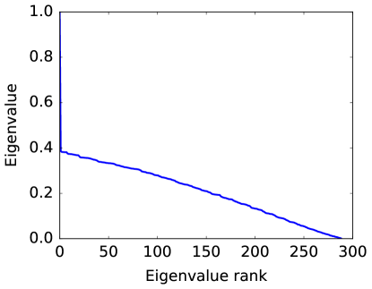
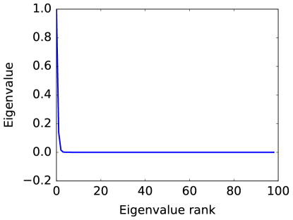
(a)	(b)

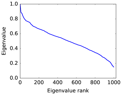
(c)

Figure 1: Spectra for three example chains: (a) Metropolis-Hastings for Bayesian logistic regression; (b) collapsed Gibbs sampler for missing data imputation; and (c) collapsed Gibbs sampler for a mixture model.

4.1 Bayesian logistic regression

Our first example is a Bayesian logistic regression problem introduced by Robert and Casella [28]. The data consists of $23$ observations of temperatures (in Fahrenheit, but normalized by dividing by $100$) and a corresponding binary outcome—failure $(y=1)$ or not $(y=0)$ of a certain component; the aim is to fit a logistic regressor, with parameters $\big{(}\alpha,~{}\beta\big{)}\in\mathbb{R}^{2}$, to the data, incorporating a prior and integrating over the model uncertainty to obtain future predictions. More explicitly, following the analysis in Gyori and Paulin [14], we consider the following model:

$$p\big{(}\alpha,~{}\beta~{}|~{}b\big{)} =\frac{1}{b}\cdot e^{\alpha}\exp\big{(}-e^{\alpha}/b\big{)}$$

$$p\big{(}y\,\mid\,\alpha,~{}\beta,~{}x\big{)} \propto\exp\big{(}\alpha+\beta x\big{)},$$

which corresponds to an exponential prior on $e^{\alpha}$, an improper uniform prior on $\beta$ and a logit link for prediction. As in Gyori and Paulin [14], we target the posterior by running a Metropolis-Hastings algorithm with a Gaussian proposal with covariance matrix $\Sigma~{}=~{}\begin{pmatrix}4&0\\ 0&10\end{pmatrix}.$ Unlike in their paper, however, we discretize the state space to facilitate exact analysis of the transition matrix and to make our theory directly applicable. The resulting state space is given by

$$\Omega=\Big{\{}\big{(}\hat{\alpha}\pm i\cdot\Delta,~{}\hat{\beta}\pm j\cdot\Delta\big{)}\,\mid\,0\leq i,~{}j\leq 8\Big{\}},$$

where $\Delta=0.1$ and $(\hat{\alpha},~{}\hat{\beta})$ is the MLE. This space has $d=17^{2}=289$ elements, resulting in a $289\times 289$ transition matrix that can easily be diagonalized.

Robert and Casella [28] analyze the probability of failure when the temperature $x$ is $$65\text{\,}\mathrm{\SIUnitSymbolDegree}$\mathrm{F}$; it is specified by the function

$$f_{65}\big{(}\alpha,~{}\beta\big{)}=\frac{\exp\big{(}\alpha+0.65\beta\big{)}}{1+\exp\big{(}\alpha+0.65\beta\big{)}}.$$

Note that this function fluctuates significantly under the posterior, as shown in Figure 2.

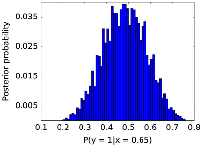
Figure 2: Distribution of $f_{65}$ values under the posterior. Despite the discretization and truncation to a square, it generally matches the one displayed in Figure 1.2 in Robert and Casella [28].

We find that this function also happens to exhibit rapid mixing. The discrepancy $d_{f_{65}}$, before entering an asymptotic regime in which it decays exponentially at a rate $1-\gamma^{\ast}\approx 0.386$, first drops from about $0.3$ to about $0.01$ in just $2$ iterations, compared to the predicted $10$ iterations from the naive bound $d_{f}\big{(}n\big{)}\leq d_{\mathrm{TV}}\big{(}n\big{)}\leq\frac{1}{\sqrt{\pi_{\mathrm{min}}}}\cdot\big{(}1-\gamma^{\ast}\big{)}^{n}.$ Figure 3 demonstrates this on a log scale, comparing the naive bound to a version of the bound in Lemmas 1 and 2. Note that the oracle $f$-discrepancy bound improves significantly over the uniform baseline, even though the non-oracle version does not. In this calculation, we took $J=\big{\{}2,\dots,140\big{\}}$ to include the top half of the spectrum excluding $1$ and computed $\ \|h_{j}\|_{\infty}$ directly from $P$ for $j\in J$ and likewise for $q_{j}^{T}f_{65}$. The oracle bound is given by Lemma 2. As shown in panel (b) of Figure 3, this decay is also faster than that of the total variation distance.

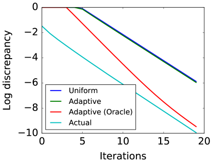
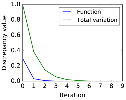
(a)	(b)

Figure 3: (a) Discrepancies (plotted on log-scale) for $f_{65}$ as a function of iteration number. The prediction of the naive bound is highly pessimistic; the $f$-discrepancy bound goes part of the way toward closing the gap and the oracle version of the $f$-discrepancy bound nearly completely closes the gap in the limit and also gets much closer to the right answer for small iteration numbers. (b) Comparison of the function discrepancy $d_{f_{65}}$ and the total variation discrepancy $d_{\mathrm{TV}}$. They both decay fairly quickly due to the large spectral gap, but the function discrepancy still falls much faster.

An important point is that the quality of the $f$-discrepancy bound depends significantly on the choice of $J$. In the limiting case where $J$ includes the whole spectrum below the top eigenvalue, the oracle bound becomes exact. Between that and $J=\emptyset$, the oracle bound becomes tighter and tighter, with the rate of tightening depending on how much power the function has in the higher versus lower eigenspaces. Figure 4 illustrates this for a few settings of $J$, showing that although for this function and this chain, a comparatively large $J$ is needed to get a tight bound, the oracle bound is substantially tighter than the uniform and non-oracle $f$-discrepancy bounds even for small $J$.

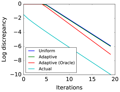
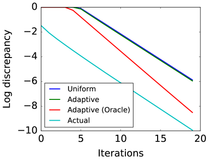
(a)	(b)
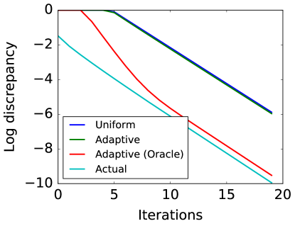
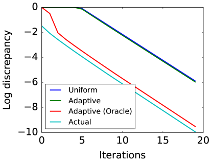
(c)	(d)

Figure 4: Comparisons of the uniform, non-oracle function-specific, and oracle function-specific bounds for various choices of $J$. In each case, $J=\{2,\dots,J_{\tiny{\mbox{max}}}\}$, with $J_{\tiny{\mbox{max}}}=50$ in panel (a), $J_{\tiny{\mbox{max}}}=100$ in panel (b), $J_{\tiny{\mbox{max}}}=200$ in panel (c), and $J_{\tiny{\mbox{max}}}=288$ in panel (d). The oracle bound becomes tight in the limit as $J_{\tiny{\mbox{max}}}$ goes to $d=289$, but it offers an improvement over the uniform bound across the board.

4.2 Bayesian analysis of clinical trials

The problem of missing data often necessitates Bayesian analysis, particularly in settings where uncertainty quantification is important, as in clinical trials. We illustrate how our framework would apply in this context by considering a clinical trials dataset [3, 14].

The dataset consists of $n=50$ patients, some of whom participated in a trial for a drug and exhibited early indicators ($Y_{i}$) of success/failure and final indicators ($X_{i}$) of success/failure. Among the 50 patients, both indicator values are available for $n_{X}=20$ patients; early indicators are available for $n_{Y}=20$ patients; and no indicators are available for $n_{0}=10$ patients. The analysis depends on the following parameterization:

$$\mathbb{P}\big{(}X_{i}=1~{}\mid~{}Y_{i}=0\big{)} =\gamma_{0},$$

$$\mathbb{P}\big{(}X_{i}=1~{}\mid~{}Y_{i}=1\big{)} =\gamma_{1},$$

$$\mathbb{P}\big{(}X_{i}=1~{}\mid~{}Y_{i}~{}\text{missing}\big{)} =p.$$

Note that, in contrast to what one might expect, $p$ is to be interpreted as the marginal probability that $X_{i}=1$, so that in actuality $p=\mathbb{P}\big{(}X_{i}=1\big{)}$ unconditionally; we keep the other notation, however, for the sake of consistency with past work [3, 14]. Conjugate uniform (i.e., $\mathrm{Be}\big{(}1,~{}1\big{)}$) priors are placed on all the model parameters.

The unknown variables include the parameter triple $\big{(}\gamma_{0},~{}\gamma_{1},~{}p\big{)}$ and the unobserved $X_{i}$ values for $n_{Y}+n_{0}=30$ patients, and the full sample space is therefore $\tilde{\Omega}=[0,~{}1]^{3}\times\big{\{}0,~{}1\big{\}}^{30}$. We cannot estimate the transition matrix for this chain, even with a discretization with as coarse a mesh as $\Delta=0.1$, since the number of states would be $d=10^{3}\times 2^{30}\sim 10^{12}$. We therefore make two changes to the original MCMC procedure. First, we collapse out the $X_{i}$ variables to bring the state space down to $[0,~{}1]^{3}$; while analytically collapsing out the discrete variables is impossible, we can estimate the transition probabilities for the collapsed chain analytically by sampling the $X_{i}$ variables conditional on the parameter values and forming a Monte Carlo estimate of the collapsed transition probabilities. Second, since the function of interest in the original work—namely, $f\big{(}\gamma_{0},~{}\gamma_{1},~{}p\big{)}=\boldsymbol{1}\big{(}p>0.5\big{)}$—depends only on $p$, we fix $\gamma_{0}$ and $\gamma_{1}$ to their MLE values and sample only $p$, restricted to the unit interval discretized with mesh $\Delta=0.01$.

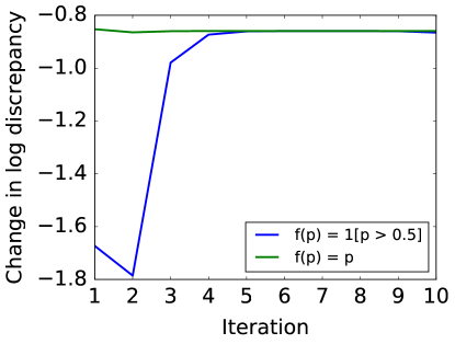
Figure 5: Change in log discrepancy for the two functions $f(p)=\boldsymbol{1}\big{(}p\geq 0.5\big{)}$ and $f(p)=p$ considered above. Whereas $f(p)=p$ always changes at the constant rate dictated by the spectral gap, the indicator discrepancy decays more quickly in the first few iterations.

As Figure 1 shows, eigenvalue decay occurs rapidly for this sampler, with $\gamma^{\ast}\approx 0.86$. Mixing thus occurs so quickly that none of the bounds—uniform or function-specific—get close to the truth, due to the presence of the constant terms (and specifically the large term $\frac{1}{\sqrt{\pi_{\mathrm{min}}}}\approx 2.14\times 10^{33}$). Nonetheless, this example still illustrates how in actual fact, the choice of target function can make a big difference in the number of iterations required for accurate estimation; indeed, if we consider the two functions

$$f_{1}(p):\,=\boldsymbol{1}\big{(}p>0.5\big{)},\quad\mbox{and}\quad f_{2}(p):\,=p,$$

we see in Figure 5 that the mixing behavior differs significantly between them: whereas the discrepancy for the second decays at the asymptotic exponential rate from the outset, the discrepancy for the first decreases faster (by about an order of magnitude) for the first few iterations, before reaching the asymptotic rate dictated by the spectral gap.

4.3 Collapsed Gibbs sampling for mixture models

Due to the ubiquity of clustering problems in applied statistics and machine learning, Bayesian inference for mixture models (and their generalizations) is a widespread application of MCMC [10, 13, 16, 24, 25]. We consider the mixture-of-Gaussians model, applying it to a subset of the schizophrenic reaction time data analyzed in Belin and Rubin [2]. The subset of the data we consider consists of $10$ measurements, with $5$ coming from healthy subjects and $5$ from subjects diagnosed with schizophrenia. Since our interest is in contexts where uncertainty is high, we chose the $5$ subjects from the healthy group whose reaction times were greatest and the $5$ subjects from the schizophrenic group whose reaction times were smallest. We considered a mixture with $K=2$ components, viz.:

$$\mu_{b} \sim\mathcal{N}\big{(}0,~{}\rho^{2}\big{)},~{}b=0,~{}1,$$

$$\omega \sim\mathrm{Be}\big{(}\alpha_{0},~{}\alpha_{1}\big{)}$$

$$Z_{i}~{}|~{}\omega \sim\mathrm{Bern}\big{(}\omega\big{)}$$

$$X_{i}~{}|~{}Z_{i}=b,~{}\mu \sim\mathcal{N}\big{(}\mu_{b},~{}\sigma^{2}\big{)}.$$

We chose relatively uninformative priors, setting $\alpha_{0}=\alpha_{1}=1$ and $\rho=237$. Increasing the value chosen in the original analysis [2], we set $\sigma\approx 70$; we found that this was necessary to prevent the posterior from being too highly concentrated, which would be an unrealistic setting for MCMC. We ran collapsed Gibbs on the indicator variables $Z_{i}$ by analytically integrating out $\omega$ and $\mu_{0:1}$.

As Figure 1 illustrates, the spectral gap for this chain is small—namely, $\gamma_{\ast}\approx 3.83\times 10^{-4}$—yet the eigenvalues fall off comparatively quickly after $\lambda_{2}$, opening up the possibility for improvement over the uniform $\gamma_{\ast}$-based bounds. In more detail, define

$$z^{\ast}_{b} :\,=\begin{pmatrix}b&b&b&b&b&1-b&1-b&1-b&1-b&1-b\end{pmatrix},$$

corresponding to the cluster assignments in which the patient and control groups are perfectly separated (with the control group being assigned label $b$). We can then define the indicator for exact recovery of the ground truth by

$$f(z)=\boldsymbol{1}\big{(}z\in\big{\{}z_{0}^{\ast},~{}z_{1}^{\ast}\big{\}}\big{)}.$$

As Figure 6 illustrates, convergence in terms of $f$-discrepancy occurs much faster than convergence in total variation, meaning that predictions of required burn-in times and sample size based on global metrics of convergence drastically overestimate the computational and statistical effort required to estimate the expectation of $f$ accurately using the collapsed Gibbs sampler. This behavior can be explained in terms of the interaction between the function $f$ and the eigenspaces of $P$. Although the pessimistic constants in the bounds from the uniform bound (10) and the non-oracle function-specific bound (Lemma 1) make their predictions overly conservative, the oracle version of the function-specific bound (Lemma 2) begins to make exact predictions after just a hundred iterations when applied with $J=\big{\{}1,\dots,25\big{\}}$; this corresponds to making exact predictions of $T_{f}\big{(}\delta\big{)}$ for $\delta\leq\delta_{0}\approx 0.01$, which is a realistic tolerance for estimation of $\mu$. Panel (b) of Figure 6 documents this by plotting the $f$-discrepancy oracle bound against the actual value of $d_{f}$ on a log scale.

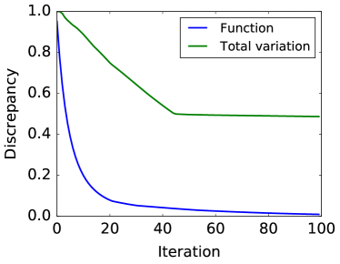
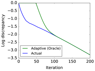
(a)	(b)

Figure 6: (a) Comparison of the $f$-discrepancy $d_{f}$ and the total variation discrepancy $d_{\mathrm{TV}}$ over the first $100$ iterations of MCMC. Clearly the function mixes much faster than the overall chain. (b) The predicted value of $\log{d_{f}}$ (according to the $f$-discrepancy oracle bound—Lemma 2) plotted against the true value. The predictions are close to sharp throughout and become sharp at around $100$ iterations.

Bound type	$T_{f}\big{(}0.01\big{)}$	$T_{f}\big{(}10^{-6}\big{)}$
Uniform	31,253	55,312
Function-Specific	25,374	49,434
Function-Specific (Oracle)	98	409
Actual	96	409

Table 1: Comparison of bounds on $T_{f}\big{(}\delta\big{)}$ for different values of $\delta$. The uniform bound corresponds to the bound $T_{f}\big{(}\delta\big{)}\leq T\big{(}\delta\big{)}$, the latter of which can be bounded by the total variation bound. The function-specific bounds correspond to Lemmas 1 and 2, respectively. Whereas the uniform and non-oracle $f$-discrepancy bounds make highly conservative predictions, the oracle $f$-discrepancy bound is nearly sharp even for $\delta$ as large as $0.01$.

The mixture setting also provides a good illustration of how the function-specific Hoeffding bounds can substantially improve on the uniform Hoeffding bound. In particular, let us compare the $T_{f}$-based Hoeffding bound (Theorem 1) to the uniform Hoeffding bound established by Léon and Perron [20]. At equilibrium, the penalty for non-independence in our bounds is $(2T_{f}(\epsilon/2))^{-1}$ compared to roughly $\gamma^{-1}_{\ast}$ in the uniform bound. Importantly, however, our concentration bound applies unchanged even when the chain has not equilibrated, provided it has approximately equilibrated with respect to $f$. As a consequence, our bound only requires a burn-in of $T_{f}(\epsilon/2)$, whereas the uniform Hoeffding bound does not directly apply for any finite burn-in. Table 1 illustrates the size of these burn-in times in practice. This issue can be addressed using the method of Paulin [27], but at the cost of a burn-in dependent penalty $d_{\mathrm{TV}}(T_{0})=\sup_{\pi_{0}}d_{\mathrm{TV}}(\pi_{n},~{}\pi)$:

$$\mathbb{P}\Big{[}\frac{1}{N-T_{0}}\sum_{n=T_{0}}^{N}f(X_{n})\geq\mu+\epsilon\Big{]}\leq d_{\mathrm{TV}}\big{(}T_{0}\big{)}+\exp\Big{\{}-\frac{\gamma_{0}}{2\big{(}1-\gamma_{0}\big{)}}\cdot\epsilon^{2}\big{[}N-T_{0}\big{]}\Big{\}},$$ (40)

where we have let $T_{0}$ denote the burn-in time. Note that a matching bound holds for the lower tail. For our experiments, we computed the tightest version of the bound (40), optimizing $T_{0}$ in the range $\big{[}0,~{}10^{5}\big{]}$ for each value of the deviation $\epsilon$. Even given this generosity toward the uniform bound, the function-specific bound still outperforms it substantially, as Figure 7 shows.

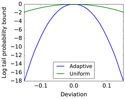
Figure 7: Comparison of the (log) tail probability bounds provided by the uniform Hoeffding bound due to [20] with one version of our function-specific Hoeffding bound (Theorem 1). Plots are based on $N=10^{6}$ iterations, and choosing the optimal burn-in for the uniform bound and a fixed burn-in of $409\geq T_{f}\big{(}10^{-6}\big{)}$ iterations for the function-specific bound. The function-specific bound improves over the uniform bound by orders of magnitude.

For the function-specific bound, we used the function-specific oracle bound (Lemma 2) to bound $T_{f}\big{(}\frac{\epsilon}{2}\big{)}$; this nearly coincides with the true value when $\epsilon\approx 0.01$ but deviates slightly for larger values of $\epsilon$.

5 Proofs of main results

This section is devoted to the proofs of the main results of this paper.

5.1 Proof of Theorem 1

We begin with the proof of the master Hoeffding bound from Theorem 1. At the heart of the proof is the following bound on the moment-generating function (MGF) for the sum of an appropriately thinned subsequence of the function values $\{f(X_{n})\}_{n=1}^{\infty}$. In particular, let us introduce the shorthand notation $\widetilde{X}_{m,t}:\,=X_{(m-1)T_{f}(\epsilon/2)+t}$ and $N_{0}:\,=N/T_{f}(\frac{\epsilon}{2})$. With this notation, we have the following auxiliary result:

Lemma 3 (Master MGF bound).

For any scalars $\beta\in\mathbb{R}$, $\epsilon\in(0,1)$, and integer $t\in\big{[}0,T_{f}(\frac{\epsilon}{2})\big{)}$, we have

$$\mathbb{E}\left[\exp\Big{(}\beta\sum_{m=1}^{N_{0}}f\big{(}\widetilde{X}_{m,t}\big{)}\Big{)}\right] \leq\exp\left\{\big{[}\frac{1}{2}\beta\epsilon+\beta\mu+\frac{1}{2}\beta^{2}\big{]}\cdot N_{0}\right\}.$$ (41)

See Section 5.1.1 for the proof of this claim. Recalling the definition of $\widetilde{X}_{m,t}$, we have

$$\mathbb{E}\left[e^{\alpha\sum_{n=1}^{N}f(X_{n})}\right] =\mathbb{E}\left[\exp\Big{\{}\alpha\sum_{t=1}^{T_{f}(\epsilon/2)}\sum_{m=1}^{N_{0}}f(\widetilde{X}_{m,t})\Big{\}}\right]$$

$$=\mathbb{E}\left[\exp\Big{\{}\alpha T_{f}(\epsilon/2)\big{[}\frac{1}{T_{f}(\epsilon/2)}\sum_{t=1}^{T_{f}(\epsilon/2)}\sum_{m=1}^{N_{0}}f(\widetilde{X}_{m,t})\big{]}\Big{\}}\right]$$

$$\leq\frac{1}{T_{f}\big{(}\epsilon/2\big{)}}\sum_{t=0}^{T_{f}\big{(}\epsilon/2\big{)}-1}\mathbb{E}\left[\exp\Big{\{}\alpha T_{f}\big{(}\epsilon/2\big{)}\sum_{m=1}^{N_{0}}f\big{(}\widetilde{X}_{m,t}\big{)}\Big{\}}\right],$$

where the last inequality follows from Jensen’s inequality, as applied to the exponential function. Applying Lemma 3 with $\beta=\alpha T_{f}\big{(}\epsilon/2\big{)}$, we conclude

$$\mathbb{E}\big{[}e^{\alpha\sum_{n=1}^{N}f(X_{n})}\big{]}\leq\exp\Big{\{}\big{[}\frac{1}{2}\alpha T_{f}\big{(}\frac{\epsilon}{2}\big{)}\epsilon+\alpha T_{f}\big{(}\frac{\epsilon}{2}\big{)}\mu+\frac{1}{2}\alpha^{2}T_{f}^{2}\big{(}\frac{\epsilon}{2}\big{)}\big{]}\cdot N_{0}\Big{\}},$$

valid for $\alpha>0$. By exponentiating and applying Markov’s inequality, it follows that

$$\mathbb{P}\left[\frac{1}{N}\sum_{n=1}^{N}f\big{(}X_{n}\big{)}\geq\mu+\epsilon\right] \leq e^{-\alpha(\mu+\epsilon)}\mathbb{E}\big{[}e^{\alpha\sum_{n=1}^{N}f(X_{n})}\big{]}$$

$$\leq\exp\left\{\frac{1}{2}\cdot\Big{[}-\alpha\>T_{f}(\frac{\epsilon}{2})\epsilon+\alpha^{2}\>T_{f}^{2}(\frac{\epsilon}{2})\Big{]}\>N_{0}(\frac{\epsilon}{2})\right\}.$$

The proof of Theorem 1 follows by taking $\alpha=\frac{\epsilon}{2T_{f}\left(\frac{\epsilon}{2}\right)}$ since

$$\mathbb{P}\left[\frac{1}{N}\sum_{n=1}^{N}f\big{(}X_{n}\big{)}\geq\mu+\epsilon\right] \leq\exp\left\{\frac{1}{2}\cdot\big{[}-\frac{\epsilon^{2}}{2}+\frac{\epsilon^{2}}{4}\big{]}\cdot N_{0}\right\}$$

$$\leq\exp\left\{-\frac{\epsilon^{2}N_{0}}{8}\right\}$$

$$=\exp\left\{-\frac{\epsilon^{2}N}{8T_{f}\big{(}\frac{\epsilon}{2}\big{)}}\right\}.$$

5.1.1 Proof of Lemma 3

For the purposes of the proof, fix $t$ and let $W_{m}=\tilde{X}_{m,t}$. For convenience, also define a dummy constant random variable $W_{0}:\,=0$. Now, by assumption, we have

$$\left|\mathbb{E}\left[f\left(W_{1}\right)\right]-\mu\right|\leq\frac{\epsilon}{2}~{}~{}\text{and}~{}~{}\left|\mathbb{E}\left[f\left(W_{m+1}\right)~{}|~{}W_{m}\right]-\mu\right|\leq\frac{\epsilon}{2}.$$

We therefore have the bound

$$\mathbb{E}\left[e^{\alpha\sum_{m}f\left(W_{m}\right)}\right] \leq\mathbb{E}\left[\prod_{m=1}^{N_{0}}e^{\alpha\left[f\left(W_{m}\right)-\mathbb{E}\left[f\left(W_{m}\right)~{}|~{}W_{m-1}\right]\right]}\right]\cdot e^{\alpha\mu N_{0}+\frac{\alpha\epsilon N_{0}}{2}}.$$ (42)

But now observe that the random variables $\Delta_{m}=f\left(W_{m}\right)-\mathbb{E}\left[f\left(W_{m}\right)~{}|~{}W_{m-1}\right]$ are deterministically bounded in $[-1,~{}1]$ and zero mean conditional on $W_{m-1}$. Moreover, by the Markovian property, this implies that the same is true conditional on $W_{<m}:\,=W_{0:\left(m-1\right)}$. It follows by standard MGF bounds that

$$\mathbb{E}\left[e^{\alpha\Delta_{m}}~{}|~{}W_{<m}\right]\leq e^{\frac{\alpha^{2}}{2}}.$$

Combining this bound with inequality (42), we conclude that

$$\mathbb{E}\left[e^{\alpha\sum_{m}f\left(W_{m}\right)}\right] \leq e^{\frac{\alpha^{2}}{2}\cdot N_{0}}\cdot e^{\alpha\mu N_{0}+\frac{\alpha\epsilon N_{0}}{2}},$$

as claimed.

5.2 Proofs of Corollaries 1 and 2

In this section, we prove the derived Hoeffing bounds stated in Corollaries 1 and 2.

5.2.1 Proof of Corollary 1

The proof is a direct application of Theorem 1. Indeed, it suffices to note that if $\epsilon\leq\frac{2\lambda_{f}}{\sqrt{\pi_{\mathrm{min}}}}$, then

$$T_{f}\big{(}\frac{\epsilon}{2}\big{)}\leq\frac{\log\big{(}\frac{2}{\epsilon\sqrt{\pi_{\mathrm{min}}}}\big{)}}{\log\big{(}\frac{1}{\lambda_{f}}\big{)}}=\frac{\log\big{(}\frac{2}{\epsilon}\big{)}+\frac{1}{2}\log\big{(}\frac{1}{\pi_{\mathrm{min}}}\big{)}}{\log\big{(}\frac{1}{\lambda_{f}}\big{)}},$$

which yields the first bound. Turning to the second bound, note that if $\epsilon>\frac{2\lambda_{f}}{\sqrt{\pi_{\mathrm{min}}}}$, then equation (12) implies that $T_{f}\big{(}\frac{\epsilon}{2}\big{)}=1$, which establishes the claim.

5.2.2 Proof of Corollary 2

The proof involves combining Theorem 1 with Lemma 1, using the setting $\epsilon=2\left(\Delta+\Delta_{J}\right)$. We begin by combining the bounds $\lambda_{J}\leq 1$, $d_{\mathrm{TV}}\left(\pi_{0},~{}\pi_{n}\right)\leq 1$, $d_{f}\left(\pi_{0},~{}\pi_{n}\right)\leq 1$, and $\mathbb{E}_{\pi}\left[f^{2}\right]\leq 1$ with the claim of Lemma 1 so as to find that

$$d_{f}\left(\pi_{0},~{}\pi_{n}\right) \leq\Delta_{J}^{\ast}+\frac{\lambda_{-J}^{n}}{\sqrt{\pi_{\mathrm{min}}}}\;\leq\;\Delta_{J}+\frac{\lambda_{-J}^{n}}{\sqrt{\pi_{\mathrm{min}}}}.$$

It follows that

$$T_{f}(\frac{\epsilon}{2}) =T_{f}\left(\Delta_{J}+\Delta\right)\leq\frac{\log\left(\frac{1}{\Delta}\right)+\frac{1}{2}\log\left(\frac{1}{\pi_{\mathrm{min}}}\right)}{\log(\frac{1}{\lambda_{-J}})}\qquad\mbox{whenever $\Delta\leq\frac{\lambda_{-J}}{\sqrt{\pi_{\mathrm{min}}}}$.}$$

Plugging into Theorem 1 now yields the first part of the bound. On the other hand, if $\Delta>\frac{\lambda_{-J}}{\sqrt{\pi_{\mathrm{min}}}}$, then Lemma 1 implies that $T_{f}\left(\Delta_{J}+\Delta\right)=1$, which proves the bound in the second case.

5.3 Proof of Proposition 1

In order to prove the lower bound in Proposition 1, we first require an auxiliary lemma:

Lemma 4.

Fix a function $\delta\colon\left(0,~{}1\right)\rightarrow\left(0,~{}1\right)$ with $\delta\left(\epsilon\right)>\epsilon$. For every constant $c_{0}\geq 1$, there exists a Markov chain $P_{c_{0}}$ and a function $f_{\epsilon}$ on it such that $\mu=\frac{1}{2}$, yet, for $N=c_{0}T_{f}\left(\delta\left(\epsilon\right)\right)$, and starting the chain from stationarity,

$$\mathbb{P}_{\pi}\left(\left|\frac{1}{N}\sum_{n=1}^{N}f_{\epsilon}\left(X_{n}\right)-\frac{1}{2}\right|\geq\epsilon\right)\geq\frac{1}{3}.$$

Using this lemma, let us now prove Proposition 1. Suppose that we make the choices

$$c_{0} :\,=\left\lceil\frac{\log 7}{c_{1}\epsilon^{2}}\right\rceil\geq 1,\quad\mbox{and}\quad N_{c_{1},\epsilon}:\,=c_{0}T_{f}\left(\epsilon\right),$$

in Lemma 4. Letting $P_{c_{0}}$ be the corresponding Markov chain and $f_{\epsilon}$ the function guaranteed by the lemma, we then have

$$\mathbb{P}_{\pi}\left(\left|\frac{1}{N_{c_{1},\epsilon}}\sum_{n=1}^{N_{c_{1},~{}\epsilon}}f_{\epsilon}\left(X_{n}\right)-\frac{1}{2}\right|\geq\epsilon\right) \geq\frac{1}{3}\;>\;\frac{2}{7}\;\geq\;2\cdot\exp\left(-\frac{c_{1}N_{c_{1},\epsilon}\epsilon^{2}}{T_{f}\left(\delta(\epsilon)\right)}\right).$$

Proof of Lemma 4:

It only remains to prove Lemma 4, which we do by constructing pathological function on a chain graph, and letting our Markov chain be the lazy random walk on this graph. For the proof, fix $\epsilon>0$, let $\delta=\delta\left(\epsilon\right)$ and let $T_{f}=T_{f}\left(\delta\right)$. Now choose an integer $d>0$ such that $d>2c_{0}$ and let the state space be $\Omega$ be the line graph with $2d$ elements with the standard lazy random walk defining $P$. We then set

$$f\left(i\right) =\begin{cases}\frac{1}{2}-\delta&~{}1\leq i\leq d,\\ \frac{1}{2}+\delta&~{}d+1\leq i\leq 2d.\end{cases}$$

It is then clear that $T_{f}=1$.

Define the bad event

$$\mathcal{E}=\left\{X_{1}\in\left[0,~{}\frac{d}{2}\right]\cup\left[\frac{3d}{2},~{}2d\right]\right\}.$$

When this occurs, we have

$$\left|\frac{1}{N^{\prime}}\sum_{n=1}^{N^{\prime}}f\left(X_{n}\right)-\frac{1}{2}\right|\geq\delta>\epsilon\qquad\mbox{with probability one},$$

for all $N^{\prime}<\frac{d}{2}$. Since $N=c_{0}<\frac{d}{2}$, we can set $N^{\prime}=N$.

On the other hand, under $\pi$, the probability of $\mathcal{E}$ is $\geq\frac{1}{3}$. (It is actually about $\frac{1}{2}$, but we want to ignore edge cases.) The claim follows immediately.

5.4 Proofs of confidence interval results

Here we provide the proof of the confidence interval corresponding to our bound (Theorem 2). Proofs of the claims (26b) and (30) can be found in Appendix C.

As discussed in Section 3.1, we actually prove a somewhat stronger form of Theorem 2, in order to guarantee that the confidence interval can be straightforwardly built using an upper bound $\tilde{T}_{f}$ on the $f$-mixing time rather than the true value. Setting $\tilde{T}_{f}=T_{f}$ recovers the original theorem.

Specifically, suppose $\tilde{T}_{f}\colon\mathbb{N}\rightarrow\mathbb{R}_{+}$ is an upper bound on $T_{f}$ and note that the corresponding tail bound becomes $e^{-\tilde{r}_{N}(\epsilon)/8}$, where

$$\tilde{r}_{N}(\epsilon)=\epsilon^{2}\left[\frac{N}{\tilde{T}_{f}\big{(}\frac{\epsilon}{2}\big{)}}-1\right].$$

This means that, just as before we wanted to make the rate $r_{N}$ in equation (27) at least as large as $8\log\frac{2}{\alpha}$, we now wish to do the same with $\tilde{r}_{N}$, which means choosing $\epsilon_{N}$ with $\tilde{r}_{N}\big{(}\epsilon_{N}\big{)}\geq 8\log\frac{2}{\alpha}$. We therefore have the following result.

Proposition 2.

For any width $\epsilon_{N}\in\tilde{r}_{N}^{-1}\big{(}\big{[}8\log\big{(}2/\alpha\big{)},~{}\infty\big{)}\big{)}$, the set

$$I^{\mathrm{func}}_{N}=\left[\frac{1}{N-T_{f}\big{(}\frac{\epsilon}{2}\big{)}}\sum_{n=\tilde{T}_{f}\big{(}\frac{\epsilon}{2}\big{)}}^{N}f\big{(}X_{n}\big{)}\pm\epsilon_{N}\right]$$

is a $1-\alpha$ confidence interval for $\mu=\mathbb{E}_{\pi}\big{[}f\big{]}$.

Proof.

For notational economy, let us introduce the shorthands $\tau_{f}(\epsilon)=T_{f}\big{(}\frac{\epsilon}{2}\big{)}$ and $\tilde{\tau}_{f}\big{(}\epsilon\big{)}=\tilde{T}_{f}\big{(}\frac{\epsilon}{2}\big{)}$. Theorem 1 then implies

$$\mathbb{P}\left[\frac{1}{N-\tilde{\tau}_{f}}\sum_{n=\tilde{\tau}_{f}}^{N}f\big{(}X_{n}\big{)}\geq\mu+\epsilon\right] \leq\exp\big{(}-\frac{N-\tau_{f}}{4\tau_{f}}\cdot\epsilon^{2}\big{)}$$

$$\leq\exp\big{(}-\frac{N-\tilde{\tau}_{f}}{4\tilde{\tau}_{f}}\cdot\epsilon^{2}\big{)}$$

$$=\exp\big{(}-\frac{\tilde{r}_{N}\big{(}\epsilon\big{)}}{4}\big{)}.$$

Setting $\epsilon=\epsilon_{N}$ yields

$$\mathbb{P}\left[\frac{1}{N-\tilde{\tau}_{f}}\sum_{n=\tilde{\tau}_{f}}^{N}f\big{(}X_{n}\big{)}\geq\mu+\epsilon_{N}\right] \leq\frac{\alpha}{2}.$$

The corresponding lower bound leads to an analogous bound on the lower tail. ∎

As we did with Corollary 3, we can derive a more concrete, though slightly weaker, form of this result that is more amenable to interpretation. We derive the corollary from the specialized bound by setting $\tilde{T}_{f}=T_{f}$.

To obtain this bound, define the following lower bound, in parallel with equation (28):

$$\tilde{r}_{N}\big{(}\epsilon\big{)}\geq\tilde{r}_{N,\eta}\big{(}\epsilon\big{)}:\,=\epsilon^{2}\big{[}\frac{N}{\tilde{T}_{f}\big{(}\frac{\eta}{2}\big{)}}-1\big{]},~{}\epsilon\geq\eta.$$

Since this is a lower bound, we see that whenever $\epsilon_{N}\geq\eta$ and $\tilde{r}_{N,\eta}\big{(}\epsilon_{N}\big{)}\geq 8\log\frac{2}{\alpha}$, $\epsilon_{N}$ is a valid half-width for a $\big{(}1-\alpha\big{)}$-confidence interval for the stationary mean centered at the empirical mean. More formally, we have the following:

Proposition 3.

Fix $\eta>0$ and let

$$\epsilon_{N}=\tilde{r}_{N,\eta}^{-1}\big{(}8\log\frac{2}{\alpha}\big{)} =2\sqrt{2}\sqrt{\frac{\tilde{T}_{f}\big{(}\frac{\eta}{2}\big{)}\cdot\log\big{(}2/\alpha\big{)}}{N-\tilde{T}_{f}\big{(}\frac{\eta}{2}\big{)}}}.$$

If $N\geq\tilde{T}_{f}\big{(}\frac{\eta}{2}\big{)}$, then $I^{\mathrm{func}}_{N}$ is a $1-\alpha$ confidence interval for $\mu=\mathbb{E}_{\pi}\big{[}f\big{]}$.

Proof.

By assumption, we have

$$\eta\leq\epsilon_{N}\big{(}\eta\big{)}=2\sqrt{\frac{\tilde{T}_{f}\big{(}\frac{\eta}{2}\big{)}\cdot\log\big{(}2/\alpha\big{)}}{N-\tilde{T}_{f}\big{(}\frac{\eta}{2}\big{)}}}.$$

This implies $\tilde{T}_{f}\big{(}\frac{\epsilon_{N}}{2}\big{)}\geq\tilde{T}_{f}\big{(}\frac{\eta}{2}\big{)}$, which yields

$$\tilde{r}_{N}\big{(}\epsilon_{N}\big{)}=\epsilon_{N}^{2}\big{[}\frac{N}{\tilde{T}_{f}\big{(}\frac{\epsilon_{N}}{2}\big{)}}-1\big{]}\geq\epsilon_{N}^{2}\big{[}\frac{N}{\tilde{T}_{f}\big{(}\frac{\eta}{2}\big{)}}-1\big{]}=8\log\big{(}2/\alpha\big{)}.$$

But now Proposition 2 applies, so that we are done. ∎

5.5 Proofs of sequential testing results

In this section, we collect various proofs associated with our analysis of the sequential testing problem.

5.5.1 Proof of Theorem 3 for $\mathcal{A}_{\mathrm{fixed}}$

We provide a detailed proof when $H_{1}$ is true, in which case we have $\mu\leq r-\delta$; the proof for the other case is analogous. When $H_{1}$ is true, we need to control the probability $\mathbb{P}\big{(}\mathcal{A}_{\mathrm{fixed}}\big{(}X_{1:N}\big{)}=H_{0}\big{)}$. In order to do so, note that Theorem 1 implies that

$$\mathbb{P}\big{(}\mathcal{A}_{\mathrm{fixed}}\big{(}X_{1:N}\big{)}=H_{0}\big{)} =\mathbb{P}\big{(}\frac{1}{N}\sum_{n=1}^{N}f\big{(}X_{n}\big{)}\geq r+\delta\big{)}$$

$$\leq\mathbb{P}\big{(}\frac{1}{N}\sum_{n=1}^{N}f\big{(}X_{n}\big{)}\geq\mu+2\delta\big{)}$$

$$\leq\exp\big{(}-\frac{\delta^{2}N}{2T_{f}\big{(}\delta\big{)}}\big{)}.$$

Setting $N=\frac{2T_{f}\left(\delta\right)\log\big{(}\frac{1}{\alpha}\big{)}}{\delta^{2}}$ yields the bound $\mathbb{P}\big{(}\mathcal{A}_{\mathrm{fixed}}\big{(}X_{1:N}\big{)}=H_{0}\big{)}\leq\alpha$, as claimed.

5.5.2 Proof of Theorem 3 for $\mathcal{A}_{\mathrm{seq}}$

The proof is nearly identical to that given by [15], with $T_{f}\big{(}\delta/2\big{)}$ replacing $\frac{1}{\gamma_{0}}$. We again assume that $H_{1}$ holds, so $\mu\leq r-\delta$. In this case, it is certainly true that

$$\mathrm{err}\big{(}\mathcal{A}_{\mathrm{seq}},~{}f\big{)} =\mathbb{P}\big{(}\exists k\colon\mathcal{A}_{\mathrm{seq}}\big{(}X_{1:N_{k}}\big{)}=H_{0}\big{)}$$

$$=\mathbb{P}\big{(}\exists k\colon\frac{1}{N_{k}}\sum_{n=1}^{N_{k}}f\big{(}X_{n}\big{)}\geq r+\frac{M}{N_{k}}\big{)}$$

$$\leq\sum_{k=1}^{\infty}\mathbb{P}\big{(}\frac{1}{N_{k}}\sum_{n=1}^{N_{k}}f\big{(}X_{n}\big{)}\geq r+\frac{M}{N_{k}}\big{)}.$$

It follows by Theorem 1, with $\epsilon_{k}=\delta+\frac{M}{N_{k}}$, that

$$\mathbb{P}\big{(}\frac{1}{N_{k}}\sum_{n=1}^{N_{k}}f\big{(}X_{n}\big{)}\geq r+\frac{M}{N_{k}}\big{)} \leq\mathbb{P}\big{(}\frac{1}{N_{k}}\sum_{n=1}^{N_{k}}f\big{(}X_{n}\big{)}\geq\mu+\delta+\frac{M}{N_{k}}\big{)}$$

$$\leq\exp\big{(}-\frac{\epsilon_{k}^{2}N_{k}}{8T_{f}\big{(}\frac{\epsilon_{k}}{2}\big{)}}\big{)}$$

$$\leq\exp\big{(}-\frac{\epsilon_{k}^{2}N_{k}}{8T_{f}\big{(}\frac{\delta}{2}\big{)}}\big{)}.$$

In order to simplify notation, for the remainder of the proof, we define $\tau:\,=4T_{f}(\delta/2)$, $\beta:\,=\frac{\sqrt{\alpha\xi}}{2}$, and $\zeta_{k}:\,=\frac{\delta^{2}N_{k}}{2\tau\log(1/\beta)}$. In terms of this notation, we have $M=\frac{2\tau\log(1/\beta)}{\delta}$, and hence that

$$\exp\big{(}-\frac{\epsilon_{k}^{2}N_{k}}{2\tau}\big{)} =\exp\big{(}-\frac{1}{2\tau}\cdot\big{(}\delta^{2}N_{k}+2\delta M+\frac{M^{2}}{N_{k}}\big{)}\big{)}$$

$$=\exp\big{(}-\big{[}\frac{\delta^{2}N_{k}}{2\tau}+\log\big{(}1/\beta\big{)}+\frac{2\tau\log^{2}\big{(}1/\beta\big{)}}{\delta^{2}N_{k}}\big{]}\big{)}$$

$$=\exp\big{(}-\log\big{(}1/\beta\big{)}\big{[}1+\zeta_{k}+\zeta_{k}^{-1}\big{]}\big{)}$$

$$=\beta\cdot\exp\big{(}-\log\big{(}1/\beta\big{)}\big{[}\zeta_{k}+\zeta_{k}^{-1}\big{]}\big{)}.$$

It follows that the error probability is at most

$$\beta\sum_{k=1}^{\infty}\exp\big{(}-\log\big{(}1/\beta\big{)}\big{[}\zeta_{k}+\zeta_{k}^{-1}\big{]}\big{)}.$$

We now finish the proof using two small technical lemmas, whose proofs we defer to Appendix D.

Lemma 5.

In the above notation, we have

$$\sum_{k=1}^{\infty}\exp\Big{\{}-\log(1/\beta)\big{[}\zeta_{k}+\zeta_{k}^{-1}\big{]}\Big{\}} \leq 4\sum_{\ell=0}^{\infty}\exp\Big{\{}-\log(1/\beta)\Big{[}\big{(}1+\xi\big{)}^{\ell}+\big{(}1+\xi\big{)}^{-\ell}\Big{]}\Big{\}}.$$

Lemma 6.

For any integer $c\geq 0$, we have

$$(1+\xi)^{\ell}+(1+\xi)^{-\ell} \geq 2(c+1)\quad\mbox{for all $\ell\in\Big{[}\frac{9c}{5\xi},\frac{9(c+1)}{5\xi}\Big{)}$.}$$

Using this bound, and grouping together terms in blocks of size $\frac{9}{5\xi}$, we find that the error is at most

$$4\sum_{\ell=0}^{\infty}\exp\big{(}-\log\big{(}1/\beta\big{)}\big{[}\big{(}1+\xi\big{)}^{\ell}+\big{(}1+\xi\big{)}^{-\ell}\big{]}\big{)} \leq\frac{36}{5\xi}\cdot\sum_{c=0}^{\infty}\beta^{2\big{(}c+1\big{)}}.$$

Since both $\alpha$ and $\xi$ are at most $\frac{2}{5}$, we have $\beta=\frac{\sqrt{\alpha\xi}}{2}\leq\frac{1}{5}$, and hence the error probability is bounded as

$$\frac{36\beta}{5\xi}\sum_{c=0}^{\infty}\beta^{2\big{(}c+1\big{)}}\leq\frac{36\beta^{3}}{5\xi\big{(}1-\beta^{2}\big{)}}\leq\frac{36\beta^{2}}{25\xi\big{(}1-\beta^{2}\big{)}}\leq\frac{3\beta^{2}}{2\xi}=\frac{3\alpha}{4}<\alpha.$$

5.5.3 Proof of Theorem 3 for $\mathcal{A}_{\mathrm{hard}}$

We may assume that $H_{1}$ holds, as the other case is analogous. Under $H_{1}$, letting $k_{0}$ be the smallest $k$ such that $\epsilon_{k}<\infty$, we have

$$\mathrm{err}(\mathcal{A}_{\mathrm{hard}},~{}f) \leq\sum_{k=k_{0}}^{\infty}\mathbb{P}\left(\hat{\mu}_{N_{k}}\geq r+\epsilon_{k}\right)\;\leq\;\sum_{k=k_{0}}^{\infty}\mathbb{P}(\hat{\mu}_{N_{k}}\geq\mu+2\epsilon_{k}).$$

By Theorem 1, and the definition of $\epsilon_{k}$, we thus have

$$\mathrm{err}\left(\mathcal{A}_{\mathrm{hard}},~{}f\right)\leq\sum_{k=k_{0}}^{\infty}\exp\left(-\frac{N_{k}\epsilon_{k}^{2}}{8T_{f}\left(\frac{\epsilon_{k}}{2}\right)}\right) \leq\frac{\alpha}{2}\sum_{k=k_{0}}^{\infty}\frac{1}{k^{2}}$$

$$=\frac{\pi^{2}}{12}\,\alpha\;<\;\alpha,$$

as claimed.

5.5.4 Proof of Theorem 4 for $\mathcal{A}_{\mathrm{seq}}$

We may assume $H_{1}$ holds; the other case is analogous. Note that

$$\mathbb{E}[N] \leq N_{1}+\sum_{k=1}^{\infty}\big{(}N_{k+1}-N_{k}\big{)}\mathbb{P}\big{(}N>N_{k}\big{)}$$

$$\leq N_{1}+\sum_{k=1}^{\infty}\big{(}N_{k+1}-N_{k}\big{)}\mathbb{P}\big{(}\frac{1}{N_{k}}\sum_{n=1}^{N_{k}}f\big{(}X_{n}\big{)}\in\big{(}r-\frac{M}{N_{k}},~{}r+\frac{M}{N_{k}}\big{)}\big{)}$$

$$\leq N_{1}+\sum_{k=1}^{\infty}\big{(}N_{k+1}-N_{k}\big{)}\mathbb{P}\big{(}\frac{1}{N_{k}}\sum_{n=1}^{N_{k}}f\big{(}X_{n}\big{)}>r-\frac{M}{N_{k}}\big{)}$$

$$=N_{1}+\sum_{k=1}^{\infty}\big{(}N_{k+1}-N_{k}\big{)}\mathbb{P}\big{(}\frac{1}{N_{k}}\sum_{n=1}^{N_{k}}f\big{(}X_{n}\big{)}>\mu+\Delta-\frac{M}{N_{k}}\big{)}$$

$$\leq N_{1}+\sum_{k=1}^{\infty}\big{(}N_{k+1}-N_{k}\big{)}\exp\left\{-\frac{\big{(}\Delta N_{k}-M\big{)}_{+}^{2}}{8T_{f}\big{(}\delta/2\big{)}N_{k}}\right\}.$$

Our proof depends on the following simple technical lemma, whose proof we defer to Appendix D.3.

Lemma 7.

Under the conditions of Theorem 4, we have

$$\sum_{k=1}^{\infty}\big{(}N_{k+1}-N_{k}\big{)}\exp\left\{-\frac{\big{(}\Delta N_{k}-M\big{)}_{+}^{2}}{8T_{f}\big{(}\delta/2\big{)}N_{k}}\right\} \leq\big{(}1+\xi\big{)}\big{[}1+\int_{N_{1}}^{\infty}h(s)\mathrm{d}s\big{]},$$ (43)

where $h(s):\,=\exp\Big{\{}-\frac{(\Delta s-M)_{+}^{2}}{8T_{f}(\delta/2)s}\Big{\}}$.

Given this lemma, we then follow the argument of Gyori and Paulin [15] in order to bound the integral. We have

$$\int_{N_{1}}^{\infty}h\big{(}s\big{)}\mathrm{d}s\leq\frac{4}{\Delta}\sqrt{\frac{2T_{f}\big{(}\delta/2\big{)}M}{\Delta}+8T_{f}\big{(}\delta/2\big{)}}.$$

To conclude, note that either $r\geq\Delta$ or $1-r\geq\Delta$, since $0<\mu<1$, so that $\min\big{(}\frac{1}{r},~{}\frac{1}{1-r}\big{)}\leq\frac{1}{\Delta}$. It follows that

$$N_{1}\leq\big{(}1+\xi\big{)}N_{0}\leq\frac{(1+\xi)M}{\Delta}.$$

Combining the bounds yields the desired result.

5.5.5 Proof of Theorem 4 for $\mathcal{A}_{\mathrm{hard}}$

For concreteness, we may assume $H_{1}$ holds, as the $H_{0}$ case is symmetric. We now have that

$$\mathbb{P}\left[N\geq N_{k}\right] \leq\mathbb{P}\left[\big{|}\frac{1}{N_{k}}\sum_{n=1}^{N_{k}}f\big{(}X_{n}\big{)}-r\big{|}\leq\epsilon_{k}\right]\;\leq\;\mathbb{P}\left[\frac{1}{N_{k}}\sum_{n=1}^{N_{k}}f\big{(}X_{n}\big{)}\geq\mu+\Delta-\epsilon_{k}\right].$$

For convenience, let us introduce the shorthand

$$T_{f,k}^{+} :\,=\begin{cases}T_{f}\big{(}\frac{\Delta-\epsilon_{k}}{2}\big{)}&~{}\text{if}~{}\epsilon_{k}\leq\Delta,\\ 1&~{}\text{otherwise}.\end{cases}$$

Applying the Hoeffding bound from Theorem 1, we then find that

$$\mathbb{P}\left[N\geq N_{k}\right] \leq\exp\left\{-\frac{N_{k}}{8T_{f,k}^{+}}\cdot\big{(}\Delta-\epsilon_{k}\big{)}_{+}^{2}\right\}.$$

Observe further that

$$\mathbb{E}[N] =N_{1}+\sum_{k=1}^{\infty}\big{(}N_{k+1}-N_{k}\big{)}\mathbb{P}\big{(}N>N_{k}\big{)}$$

$$\leq N_{k_{0}^{\ast}+1}+\sum_{k=k_{0}^{\ast}+1}^{\infty}\big{(}N_{k+1}-N_{k}\big{)}\mathbb{P}\big{(}N>N_{k}\big{)}$$

$$\leq\big{(}1+\xi\big{)}\big{(}N_{0}^{\ast}+1\big{)}+\sum_{k=k_{0}^{\ast}+1}^{\infty}\big{(}N_{k+1}-N_{k}\big{)}\mathbb{P}\big{(}N>N_{k}\big{)}.$$

Combining the pieces yields

$$\mathbb{E}[N] \leq\big{(}1+\xi\big{)}\big{(}N_{0}^{\ast}+1\big{)}+\sum_{k=k_{0}^{\ast}+1}^{\infty}\big{(}N_{k+1}-N_{k}\big{)}\exp\big{(}-\frac{N_{k}}{8T_{f,k}^{+}}\cdot\big{(}\Delta-\epsilon_{k}\big{)}_{+}^{2}\big{)}.$$ (44)

The crux of the proof is a bound on the infinite sum, which we pull out as a lemma for clarity.

Lemma 8.

The infinite sum (44) is upper bounded by

$$\sum_{k=k_{0}^{\ast}+1}^{\infty}\big{(}N_{k+1}-N_{k}\big{)}\exp\big{(}-\frac{N_{k}}{8T_{f,k}^{+}}\cdot\big{(}\Delta-\epsilon_{k}\big{)}_{+}^{2}\big{)}\leq\alpha\cdot\sum_{m=1}^{\infty}\exp\big{(}-m\cdot\frac{\Delta^{2}}{32T_{f}\big{(}\frac{\Delta}{4}\big{)}}\big{)}.$$

See Appendix D.4 for the proof of this claim.

Lemma 8 then implies that

$$\sum_{k=k_{0}^{\ast}+1}^{\infty}\big{(}N_{k+1}-N_{k}\big{)}\exp\big{(}-\frac{N_{k}}{T_{f}\big{(}\frac{\Delta}{4}\big{)}}\cdot\frac{\Delta^{2}}{32}\big{)} \leq\alpha\cdot\sum_{m=1}^{\infty}\exp\big{(}-m\cdot\frac{\Delta^{2}}{32T_{f}\big{(}\frac{\Delta}{4}\big{)}}\big{)}$$

$$=\frac{\alpha\exp\big{(}-\frac{\Delta^{2}}{32T_{f}\big{(}\frac{\Delta}{4}\big{)}}\big{)}}{1-\exp\big{(}\frac{\Delta^{2}}{32T_{f}\big{(}\frac{\Delta}{4}\big{)}}\big{)}}$$

$$\leq\frac{32\alpha T_{f}\big{(}\frac{\Delta}{4}\big{)}}{\Delta^{2}}.$$

The claim now follows from equation (44).

6 Discussion

A significant obstacle to successful application of statistical procedures based on Markov chains—especially MCMC—is the possibility of slow mixing. The usual formulation of mixing is in terms of convergence in a distribution-level metric, such as the total variation or Wasserstein distance. On the other hand, algorithms like MCMC are often used to estimate equilibrium expectations over a limited class of functions. For such uses, it is desirable to build a theory of mixing times with respect to these limited classes of functions and to provide convergence and concentration guarantees analogous to those available in the classical setting, and our paper has made some steps in this direction.

In particular, we introduced the $f$-mixing time of a function, and showed that it can be characterized by the interaction between the function and the eigenspaces of the transition operator. Using these tools, we proved that the empirical averages of a function $f$ concentrate around their equilibrium values at a rate characterized by the $f$-mixing time; in so doing, we replaced the worst-case dependence on the spectral gap of the chain, characteristic of previous Markov chain concentration bounds, by an adaptive dependence on the properties of the actual target function. Our methodology yields sharper confidence intervals, as well as better rates for sequential hypothesis tests in MCMC, and we have provided evidence that the predictions made by our theory are accurate in some real examples of MCMC and thus potentially of significant practical relevance.

Our investigation also suggests a number of further questions. Two important ones concern the continuous and non-reversible cases. Both arise frequently in statistical applications—for example, when sampling continuous parameters or when performing Gibbs sampling with systematic scan—and are therefore of considerable interest. As uniform Hoeffding bounds do exist for the continuous case and, more recently, have been established for the non-reversible case, we believe many of our conclusions should carry over to these settings, although somewhat different methods of analysis may be required.

Furthermore, in practical applications, it would be desirable to have methods for estimating or bounding the $f$-mixing time based on samples. It would also be interesting to study the $f$-mixing times of Markov chains that arise in probability theory, statistical physics, and applied statistics itself. While we have shown what can be done with spectral methods, the classical theory provides a much larger arsenal of techniques, some of which may generalize to yield sharper $f$-mixing time bounds. We leave these and other problems to future work.

Acknowledgments

The authors thank Alan Sly and Roberto Oliveira for helpful discussions about the lower bounds and the sharp function-specific Hoeffding bounds (respectively). This work was partially supported by NSF grant CIF-31712-23800, ONR-MURI grant DOD 002888, and AFOSR grant FA9550-14-1-0016. In addition, MR is supported by an NSF Graduate Research Fellowship and a Fannie and John Hertz Foundation Google Fellowship.

Appendix A Proofs for Section 2.2

In this section, we gather the proofs of the mixing time bounds from Section 2.2, namely equations (10) and (12) and Lemmas 1 and 2.

A.1 Proof of the bound (10)

Recall that

$$d_{f}(p,~{}q) =\sup_{f\colon[d]\rightarrow[0,~{}1]}\left|\mathbb{E}_{p}\big{[}f\big{(}X\big{)}\big{]}-\mathbb{E}_{q}\big{[}f(Y)\big{]}\right|.$$

It follows from equation (12) that

$$d_{\mathrm{TV}}\big{(}\pi_{n},~{}\pi\big{)} =\sup_{f\colon[d]\rightarrow[0,~{}1]}d_{f}\big{(}\pi_{n},~{}\pi\big{)}$$

$$\leq\sup_{f\colon[d]\rightarrow[0,~{}1]}\big{[}\frac{\lambda_{f}^{n}}{\sqrt{\pi_{\mathrm{min}}}}\cdot d_{f}\big{(}\pi_{0},~{}\pi\big{)}\big{]}$$

$$=\frac{1}{\sqrt{\pi_{\mathrm{min}}}}\cdot\lambda_{\ast}^{n}\cdot d_{\mathrm{TV}}\big{(}\pi_{0},~{}\pi\big{)},$$

as claimed.

A.2 Proof of equation (12)

Let $D=\mathrm{diag}\big{(}\sqrt{\pi}\big{)}$. Then the matrix $A=DPD^{-1}$ is symmetric and so has an eigendecomposition of the form $A=\gamma_{1}\gamma_{1}^{T}+\sum_{j=2}^{d}\lambda_{j}\gamma_{j}\gamma_{j}^{T}$. Using this decomposition, we have

$$P=\boldsymbol{1}\pi^{T}+\sum_{j=2}^{d}\lambda_{j}h_{j}q_{j}^{T},$$

where $h_{j}:\,=D^{-1}\gamma_{j}$ and $q_{j}:\,=D\gamma_{j}$. Note that the vectors $\{q_{j}\}_{j=2}^{d}$ correspond to the left eigenvectors associated with the eigenvalues $\{\lambda_{j}\}_{j=2}^{d}$.

Now, if we let $\pi_{0}$ be an arbitrary distribution over $[d]$, we have

$$d_{f}(\pi_{n},~{}\pi) =\big{|}\pi_{0}^{T}P^{n}f-\pi^{T}P^{n}f\big{|}\;\leq\;\big{|}(\pi_{0}-\pi)^{T}P^{n}f\big{|}.$$

Defining $P_{f}:\,=\boldsymbol{1}\pi^{T}+\sum_{j\in J_{f}}\lambda_{j}h_{j}q_{j}^{T}$, we have $P^{n}f=P_{f}^{n}f$. Moreover, if we define $\tilde{P}_{f}:\,=\sum_{j\in J_{f}}\lambda_{j}h_{j}q_{j}^{T}$, and correspondingly $\tilde{A}_{f}:\,=D\tilde{P}_{f}D^{-1}$, we then have the relation $\big{(}\pi_{0}-\pi\big{)}^{T}\tilde{P}_{f}=\big{(}\pi_{0}-\pi\big{)}^{T}P_{f}$. Consequently, by the definition of the operator norm and sub-multiplicativity, we have

$$d_{f}\big{(}\pi_{n},~{}\pi\big{)} \leq\big{|}\big{(}\pi_{0}-\pi\big{)}^{T}\tilde{P}_{f}^{n}f\big{|}$$

$$\leq|\!|\!|\tilde{A}_{f}|\!|\!|_{{\tiny{\mbox{op}}}}^{n}\|Df\|_{2}\big{\|}D^{-1}\big{(}\pi_{0}-\pi\big{)}\big{\|}_{2}$$

$$=\sqrt{\mathbb{E}_{\pi}\big{[}f^{2}\big{]}\cdot\sum_{i\in[d]}\frac{\big{(}\pi_{0,i}-\pi_{i}\big{)}^{2}}{\pi_{i}}}\cdot\lambda_{f}^{n}d_{f}\big{(}\pi_{0},~{}\pi\big{)}.$$

In order to complete the proof, let $Z\in\{0,~{}1\}^{d}$ denote the indicator vector $Z_{j}=\boldsymbol{1}\big{(}X_{0}=j\big{)}$. Observe that the function

$$r(z):\,=\sum_{i\in[d]}\frac{\big{(}z_{i}-\pi_{i}\big{)}^{2}}{\pi_{i}}$$

is convex in terms of $z$. Thus, Jensen’s inequality implies that

$$\mathbb{E}_{\pi_{0}}\big{[}r(Z)\big{]}\geq r\big{(}\mathbb{E}_{\pi_{0}}\big{[}Z\big{]}\big{)}=r\big{(}\pi_{0}\big{)}=\sum_{i\in[d]}\frac{\big{(}\pi_{0,i}-\pi_{i}\big{)}^{2}}{\pi_{i}}.$$

On the other hand, for any fixed value $X_{0}=j$, corresponding to $Z=e_{j}$, we have

$$r\big{(}z\big{)}=r\big{(}e_{j}\big{)}=\frac{\big{(}1-\pi_{j}\big{)}^{2}}{\pi_{j}}+\sum_{i\neq j}\pi_{i}=\frac{1-\pi_{j}}{\pi_{j}}\leq\frac{1}{\pi_{\mathrm{min}}}.$$

We deduce that $d_{f}(\pi_{n},~{}\pi)\leq\sqrt{\frac{\mathbb{E}_{\pi}[f^{2}]}{\pi_{\mathrm{min}}}}\cdot\lambda_{f}^{n}\cdot d_{f}(\pi_{0},~{}\pi)$, as claimed.

A.3 Proof of Lemma 1

We observe that

$$\big{|}(\pi_{0}-\pi)^{T}h_{J}(n)\big{|} \leq\|\pi_{0}-\pi\|_{1}\;\|h_{J}(n)\|_{\infty}$$

$$=2d_{\mathrm{TV}}\big{(}\pi_{0},~{}\pi\big{)}\;\|h_{J}(n)\|_{\infty}$$

$$\leq 2d_{\mathrm{TV}}\big{(}\pi_{0},~{}\pi\big{)}\;\Big{\{}\sum_{j\in J}\big{|}\lambda_{j}\big{|}^{n}\cdot\big{|}q_{j}^{T}f\big{|}\cdot\|h_{j}\|_{\infty}\Big{\}}$$

$$\leq 2d_{\mathrm{TV}}\big{(}\pi_{0},~{}\pi\big{)}\;\Big{\{}2\big{|}J\big{|}\cdot\max_{j\in J}\big{|}q_{j}^{T}f\big{|}\cdot\max_{j\in J}\|h_{j}\|_{\infty}\Big{\}},$$

as claimed.

A.4 Proof of Lemma 2

We proceed in a similar fashion as in the proof of equation (12). Begin with the identity proved there, viz.

$$d_{f}\big{(}\pi_{n},~{}\pi\big{)}=\big{|}(\pi_{0}-\pi)^{T}\tilde{P}_{f}^{n}f\big{|},$$

where $\tilde{P}_{f}=\sum_{j\in J_{f}}\lambda_{j}h_{j}q_{j}^{T}$. Now decompose $\tilde{P}_{f}$ further into

$$P_{J}=\sum_{j\in J}\lambda_{j}h_{j}q_{j}^{T}~{}~{}\text{and}~{}~{}P_{-J}=\sum_{j\in J_{f}\setminus J}\lambda_{j}h_{j}q_{j}^{T}.$$

Note also that $\tilde{P}_{f}^{n}=P_{J}^{n}+P_{-J}^{n}$. We thus find that

$$d_{f}(\pi_{n},~{}\pi) \leq\big{|}(\pi_{0}-\pi)^{T}P_{J}^{n}f\big{|}+\big{|}(\pi_{0}-\pi)^{T}P_{-J}^{n}f\big{|}.$$

Now observe that $P_{J}^{n}f=h_{J}(n)$, so $\big{|}(\pi_{0}-\pi)^{T}P_{J}^{n}f\big{|}=\big{|}(\pi_{0}-\pi)^{T}h_{J}(n)|$. On the other hand, the second term can be bounded using the argument from the proof of equation (12) to obtain

$$\big{|}(\pi_{0}-\pi)^{T}P_{-J}^{n}f\big{|}\leq\sqrt{\frac{\mathbb{E}_{\pi}\big{[}f^{2}\big{]}}{\pi_{\mathrm{min}}}}\cdot\lambda_{-J_{\delta}}^{n}\cdot d_{f}(\pi_{0},~{}\pi),$$

as claimed.

Appendix B Proofs for Section 2.4

In this section, we provide detailed proofs of the bound (24), as well as the other claims about the random function example on $C_{2d}$.

Proposition 4.

Let $f\colon[d]\rightarrow[0,~{}1]$ with $f(i)\sim\tau$ iid from some distribution on $[0,~{}1]$. There exists a universal constant $c_{0}>0$ such that with probability $\geq 1-\frac{\delta^{\ast}}{128\sqrt{d\log{d}}}$ over the randomness $f$, we have

$$T_{f}\big{(}\delta\big{)}\leq\frac{c_{0}d\log{d}\log{\frac{128d}{\delta}}}{\delta^{2}}\qquad\mbox{for all $0<\delta\leq\delta^{\ast}$.}$$

Proof.

We proceed by defining a “good event” $\mathcal{E}_{\delta}$, and then showing that the stated bound on $T_{f}(\delta)$ holds conditioned on this event. The final step is to show that $\mathbb{P}[\mathcal{E}_{\delta}]$ is suitably close to one, as claimed.

The event $\mathcal{E}_{\delta}$ is defined in terms of the interaction between $f$ and the eigenspaces of $P$ corresponding to eigenvalues close to $1$. More precisely, denote the indices of these eigenvalues by

$$J_{\delta} :\,=\Big{\{}j\in\{1,\ldots,2d-1\}\;\mid\;j\leq 4\delta\sqrt{\frac{d}{\log{d}}}~{}~{}\text{or}~{}~{}j\geq 2d-4\delta\sqrt{\frac{d}{\log{d}}}\Big{\}}.$$

The good event $\mathcal{E}_{\delta}$ occurs when $f$ has small inner product with all the corresponding eigenfunctions—that is

$$\mathcal{E}_{\delta} :\,=\Big{\{}\max_{j\in J_{\delta}}|q_{j}^{T}f|\leq 2\sqrt{\frac{10\log d}{d}}\Big{\}}.$$

Viewed as family of events indexed by $\delta$, these events form a decreasing sequence. (In particular, the associated sequence of sets $J_{\delta}$ is increasing in $\delta$, in that whenever $\delta\leq\delta^{\ast}$, we are guaranteed that $J_{\delta}\subset J_{\delta^{\ast}}$.)

Establishing the bound conditionally on $\mathcal{E}_{\delta}$:

We now exploit the spectral properties of the transition matrix to bound $T_{f}$ conditionally on the event $\mathcal{E}_{\delta}$. Recall that the lazy random walk on $C_{2d}$ has eigenvalues $\lambda_{j}=\frac{1}{2}\big{(}1+\cos(\frac{\pi j}{d})\big{)}$ for $j\in[d]$, with corresponding unit eigenvectors

$$v_{j}^{T}=\frac{1}{\sqrt{2d}}\begin{pmatrix}1&\omega_{j}&\cdots&\omega_{j}^{2d-1}\end{pmatrix},~{}~{}\omega_{j}\colon=e^{\frac{\pi ij}{d}}.$$

(See  [21] for details.) We note that this diagonalization allows us to write $P=\boldsymbol{1}\pi^{T}+\sum_{j=1}^{2d-1}\lambda_{j}h_{j}q_{j}^{T}$, where $h_{j}=\sqrt{2d}\cdot v_{j}$ and $q_{j}=\frac{v_{j}}{\sqrt{2d}}$, where we have used the fact that $\mathrm{diag}\big{(}\sqrt{\pi}\big{)}=\frac{1}{\sqrt{2d}}\cdot I$. Note that $\|h_{j}\|_{\infty}=1$.

Combining Lemma 1 with the bounds $\lambda_{J_{\delta}}\leq 1$, $\|h_{j}\|_{\infty}\leq 1$, and $\big{|}J_{\delta}\big{|}\leq 8\delta\sqrt{\frac{d}{\log{d}}}$, we find that

$$d_{f}(\pi_{n},~{}\pi) \leq 16\delta\sqrt{\frac{d}{\log{d}}}\cdot\max_{j\in J}\big{|}q_{j}^{T}f\big{|}+\sqrt{d}\cdot\lambda_{-J_{\delta}}^{n}.$$

Therefore, when the event $\mathcal{E}_{\delta}$ holds, we have

$$d_{f}(\pi_{n},~{}\pi) \leq 32\sqrt{10}\cdot\delta+\sqrt{d}\cdot\lambda_{-J_{\delta}}^{n}.$$ (45)

In order to conclude the argument, we use the fact that

$$\lambda_{-J_{\delta}}=\frac{1+\max_{j\in J_{f}\setminus J_{\delta}}\cos\big{(}\frac{\pi j}{d}\big{)}}{2}\leq\frac{1+\cos\big{(}\frac{\pi j_{0}}{d}\big{)}}{2},$$

where $j_{0}=4\delta\sqrt{\frac{d}{\log{d}}}$. On the other hand, we also have

$$\cos\big{(}\pi x\big{)}\leq 1-\frac{\pi^{2}x^{2}}{2}+\frac{\pi^{4}x^{4}}{24}\leq 1-\frac{\pi^{2}x^{2}}{12},\qquad\mbox{for all $|x|\leq 1$,}$$

which implies that

$$\lambda_{-J_{\delta}}\leq 1-\frac{2\pi^{2}\delta^{2}}{3d\log{d}}\leq\exp\big{(}-\frac{2\pi^{2}\delta^{2}}{3d\log{d}}\big{)}.$$

Together with equation (45), this bound implies that for $n\geq\frac{3d\log{d}\log{\frac{d}{\delta}}}{2\pi^{2}\delta^{2}}$, we have $\sqrt{d}\lambda_{-J_{\delta}}^{n}\leq\delta$, whence

$$d_{f}(\pi_{n},~{}\pi)\leq(32\sqrt{10}+1)\,\delta\leq 128\delta.$$

Replacing $\delta$ by $\frac{\delta}{128}$ throughout, we conclude that for

$$n\geq\frac{3\,(128)^{2}d\log{d}\log{\frac{128d}{\delta}}}{2\pi^{2}\delta^{2}}=\frac{3\cdot 2^{13}}{\pi^{2}}\cdot\frac{d\log{d}\log\frac{128d}{\delta}}{\delta^{2}},$$

we have $d_{f}(\pi_{n},~{}\pi)\leq\delta$ with probability at least $\mathbb{P}\left(\mathcal{E}_{\delta/128}\right)$.

Controlling the probability of $\mathcal{E}_{\delta}$:

It now suffices to prove $\mathbb{P}(\mathcal{E}_{\delta})\geq 1-\frac{\delta}{\sqrt{d\log{d}}}$, since this implies that $\mathbb{P}\left(\mathcal{E}_{\delta/128}\right)\geq 1-\frac{\delta}{128\sqrt{d\log{d}}}$, as required. In order to do so, observe that the vectors $\{q_{j}\}_{j=1}^{d}$ are rescaled versions of an orthonormal collection of eigenvectors, and hence

$$\mathbb{E}\big{[}q_{j}^{T}f\big{]}=\mathbb{E}_{\nu}\left[\mu\right]\cdot q_{j}^{T}\boldsymbol{1}=0.$$

We can write the inner product as $q_{j}^{T}f=A_{j}+iB_{j}$, where $(A_{j},B_{j})$ are a pair of real numbers. The triangle inequality then guarantees that $|q_{j}^{T}f|\leq|A_{j}|+|B_{j}|$, so that it suffices to control these two absolute values.

By definition, we have

$$A_{j}=\frac{1}{2d}\sum_{\ell=0}^{2d-1}f\big{(}\ell\big{)}\cdot\cos\big{(}\frac{\pi j\ell}{d}\big{)},$$

showing that it is the sum of sub-Gaussian random variables with parameters $\sigma_{\ell,j}^{2}=\cos^{2}\big{(}\frac{\pi j\ell}{d}\big{)}\leq 1$. Thus, the variable $A_{j}$ is sub-Gaussian with parameter at most $\sigma_{j}^{2}\leq\frac{1}{2d}$. A parallel argument applies to the scalar $B_{j}$, showing that it is also sub-Gaussian with parameter at most $\sigma_{j}^{2}$.

By the triangle inequality, we have $|q_{j}^{T}f|\leq|A_{j}|+|B_{j}|$, so it suffices to bound $\big{|}A_{j}\big{|}$ and $|B_{j}|$ separately. In order to do so, we use sub-Gaussianity to obtain

$$\mathbb{P}\big{(}\max_{j\in J}|A_{j}|\geq r\big{)} \leq|J|\cdot e^{-\frac{r^{2}}{2}}\leq 8\delta\sqrt{\frac{d}{\log{d}}}\cdot e^{-\frac{dr^{2}}{2}}.$$

With $r:\,=\sqrt{\frac{2\log{16d}}{d}}$, we have

$$\mathbb{P}\big{(}\max_{j\in J_{\delta}}\big{|}A_{j}\big{|}\geq\sqrt{\frac{2\log{16d}}{d}}\big{)}\leq\frac{\delta}{2\sqrt{d\log{d}}}.$$

Applying a similar argument to $B_{j}$ and taking a union bound, we find that

$$\mathbb{P}\big{(}\max_{j\in J_{\delta}}\big{|}q_{j}^{T}f\big{|}\geq 2\sqrt{\frac{2\log{16d}}{d}}\big{)}\leq\frac{\delta}{\sqrt{d\log{d}}}.$$

Since $2\sqrt{\frac{2\log{16d}}{d}}\leq 2\sqrt{\frac{10\log d}{d}}$ for $d\geq 2$, we deduce that

$$1-\mathbb{P}\left(\mathcal{E}_{\delta}\right)=\mathbb{P}\left(\max_{j\in J_{\delta}}\left|q_{j}^{T}f\right|\geq 2\sqrt{\frac{10\log d}{d}}\right)\leq\frac{\delta}{\sqrt{d\log{d}}},$$

as required. ∎ The concentration result now follows.

Proposition 5.

The random function $f$ on $C_{2d}$ defined in equation (21) satisfies the mixing time and tail bounds

$$T_{f}\big{(}\frac{\epsilon}{2}\big{)} \leq\frac{c_{0}d\log{d}\big{[}\log{d}+\log\big{(}\frac{1}{\epsilon^{2}}\big{)}\big{]}}{\epsilon^{2}},$$

and

$$\mathbb{P}\left[\frac{1}{N}\sum_{n=T_{f}\big{(}\epsilon/2\big{)}}^{N+T_{f}(\epsilon/2)}f\big{(}X_{n}\big{)}\geq\mu+\epsilon\right] \leq\exp\big{(}-\frac{c_{1}\epsilon^{4}N}{d\log{d}\big{[}\log(\frac{1}{\epsilon})+\log{d}\big{]}}\big{)}.$$

with probability at least $1-\frac{c_{2}\epsilon^{2}}{\sqrt{d\log{d}}}$ over the randomness of $f$ provided $\epsilon\geq c_{3}\big{(}\frac{\log{d}}{d}\big{)}^{1/2}$, where $c_{0},c_{1},c_{2},c_{3}>0$ are universal constants.

Proof.

We first note that from the proof of Proposition 4, we have the lower bound $1-\lambda_{-J_{\delta}}\geq\frac{c_{4}\delta^{2}}{d\log{d}}$, valid for all $\delta\in(0,1)$. The proof of the previous proposition guarantees that $\Delta_{J}^{\ast}\leq 32\sqrt{10}\delta$, so setting $\delta=\frac{\epsilon}{128\sqrt{10}}$ yields

$$\frac{\epsilon}{4}=32\sqrt{10}\delta\geq\Delta_{J}^{\ast},\quad\mbox{and}\quad 1-\lambda_{-J_{\delta}}\geq\frac{c_{4}^{\prime}\epsilon^{2}}{d\log{d}}.$$

Now, by Proposition 4, there is a universal constant $c_{5}>0$ such that, with probability at least $1-\frac{\delta}{128\sqrt{d\log d}}$, we have

$$T_{f}\big{(}\delta^{\prime}\big{)}\leq\frac{c_{5}d\log{d}\log{d/\delta^{\prime}}}{\big{(}\delta^{\prime}\big{)}^{2}}\qquad\mbox{for all $\delta^{\prime}\geq\delta$.}$$

In particular, we have

$$T_{f}\big{(}\frac{\epsilon}{2}\big{)}\leq\frac{c_{2}^{\prime}d\log{d}\log{d/\epsilon}}{\epsilon^{2}}$$

with this same probability. Thus, we have this bound on $T_{f}$ with the high probability claimed in the statement of the proposition.

We now finish by taking $\Delta=\frac{\epsilon}{4}$ in Corollary 2. Noting that $\Delta_{J}+\Delta=\frac{\epsilon}{2}$ and $1-\lambda_{-J}\geq\frac{c_{4}^{\prime}\epsilon^{2}}{d\log{d}}$ completes the proof. ∎

Appendix C Proofs for Section 3.1

We now prove correctness of the confidence intervals based on the uniform Hoeffding bound (5), and the Berry-Esseen bound (29).

C.1 Proof of claim (26b)

This claim follows directly from a modified uniform Hoeffding bound, due to [27]. In particular, for any integer $T_{0}\geq 0$, let $d_{\mathrm{TV}}(T_{0})=\sup_{\pi_{0}}d_{\mathrm{TV}}(\pi_{0}P^{T_{0}},~{}\pi)$ be the worst-case total variation distance from stationarity after $T_{0}$ steps. Using this notation, [27] shows that for any starting distribution $\pi_{0}$ and any bounded function $f\colon[d]\rightarrow[0,~{}1]$, we have

$$\mathbb{P}\big{(}\big{|}\frac{1}{N-T_{0}}\sum_{n=T_{0}+1}^{N}f\big{(}X_{n}\big{)}-\mu\big{|}\geq\epsilon\big{)}\leq 2\exp\big{(}-\frac{\gamma_{0}}{2\big{(}2-\gamma_{0}\big{)}}\cdot\epsilon^{2}N\big{)}+2d_{\mathrm{TV}}\big{(}T_{0}\big{)}.$$ (46)

We now use the bound (46) to prove our claim (26b). Recall that we have chosen $T_{0}$ so that $d_{\mathrm{TV}}\big{(}T_{0}\big{)}\leq\alpha_{0}/2$. Therefore, the bound (46) implies that

$$\mathbb{P}\left[\big{|}\frac{1}{N-T_{0}}\sum_{n=T_{0}+1}^{N}f(X_{n})-\mu\big{|}\geq\epsilon_{N}\right] \leq 2\exp\Big{\{}-\frac{\gamma_{0}}{2\big{(}2-\gamma_{0}\big{)}}\cdot\epsilon_{N}^{2}N\Big{\}}+\alpha_{0}$$

$$\leq 2\cdot\frac{\alpha-\alpha_{0}}{2}+\alpha_{0}=\alpha,$$

as required.

C.2 Proof of the claim (30)

We now use the result (29) to prove the claim (30).

By the lower bound on $N$, we have

$$\frac{e^{-\gamma_{0}N}}{3\sqrt{\pi_{\mathrm{min}}}}\leq\frac{\alpha}{6}~{}~{}\text{and}~{}~{}\frac{13}{\sigma_{f,\mathrm{asym}}\sqrt{\pi_{\mathrm{min}}}}\cdot\frac{1}{\gamma_{0}\sqrt{N}}\leq\frac{\alpha}{6}.$$

It follows from equation (29) that

$$\mathbb{P}\left[\frac{1}{\sigma_{f,\mathrm{asym}}N}\sum_{n=1}^{N}f\big{(}X_{n}\big{)}\geq\mu+\epsilon_{N}\right] \leq\Phi\big{(}\epsilon_{N}\sqrt{N}\big{)}+\frac{\alpha}{3}$$

$$\leq\exp\big{(}-\frac{N}{2}\cdot\epsilon_{N}^{2}\big{)}+\frac{\alpha}{3}$$

$$=\frac{\alpha}{2},$$

and since a matching bound holds for the lower tail, we get the desired result.

Appendix D Proofs for Section 5.5

In this section, we gather the proofs of Lemmas 5–8.

D.1 Proof of Lemma 5

Observe that the function

$$g(\zeta) :\,=\exp\Big{\{}-\log(1/\beta)\,(\zeta+\zeta^{-1})\Big{\}}$$

is increasing on $(0,~{}1]$ and decreasing on $[1,~{}\infty)$. Therefore, bringing $\zeta$ closer to $1$ can only increase the value of the function.

Now, for fixed $k\geq 1$, define

$$\ell_{k}:\,=\begin{cases}\min\big{\{}\ell\colon\big{(}1+\xi\big{)}^{\ell}\geq\zeta_{k}\big{\}}&~{}\text{if}~{}\zeta_{k}\leq 1,\\ \max\big{\{}\ell\colon\big{(}1+\xi\Big{)}^{\ell}\leq\zeta_{k}\big{\}}&~{}\text{otherwise.}\end{cases}$$

In words, the quantity $\ell_{k}$ is either the smallest integer such that $\big{(}1+\xi\big{)}^{\ell}$ is bigger than $\zeta_{k}$ (if $\zeta_{k}\leq 1$) or the largest integer such that $\big{(}1+\xi\big{)}^{\ell}$ is smaller than $\zeta_{k}$ (if $\zeta_{k}\geq 1$).

With this definition, we see that $\big{(}1+\xi\big{)}^{\ell_{k}}$ always lies between $\zeta_{k}$ and $1$, so that we are guaranteed that $g\big{(}\big{(}1+\xi\big{)}^{\ell_{k}}\big{)}\geq g\big{(}\zeta_{k}\big{)}$, and hence

$$\sum_{k=1}^{\infty}g\big{(}\zeta_{k}\big{)}\leq\sum_{k=1}^{\infty}g\big{(}(1+\xi)^{\ell_{k}}\big{)}.$$

Thus, it suffices to show that at most two distinct values of $k$ map to a single $\ell_{k}$. Indeed, when this mapping condition holds, we have

$$\sum_{k=1}^{\infty}g\big{(}\zeta_{k}\big{)}\leq 2\sum_{\ell=-\infty}^{\infty}g\big{(}\big{(}1+\xi\big{)}^{\ell}\big{)}\leq 4\sum_{\ell=0}^{\infty}g\big{(}\big{(}1+\xi\big{)}^{\ell}\big{)}.$$

In order to prove the stated mapping condition, note first that $\ell_{k}$ is clearly nondecreasing in $k$, so that we need to prove that $\ell_{k+2}>\ell_{k}$ for all $k\geq 1$. It is sufficent to show that $\zeta_{k+2}\geq\big{(}1+\xi\big{)}\zeta_{k}$, since this inequality implies that $\ell_{k+2}\geq\ell_{k}+1$.

We now exploit the fact that $\zeta_{k}=an_{k}$ for some absolute constant $a$, where $n_{k}=\lfloor n_{0}\big{(}1+\xi\big{)}^{k}\rfloor$. For this, let $b=n_{0}\big{(}1+\xi\big{)}^{k}$, so that $n_{k}=\lfloor b\rfloor$. Since $n_{k+1}>n_{k}$, we have $\big{(}1+\xi\big{)}b\geq\lfloor\big{(}1+\xi\big{)}b\rfloor\geq\lfloor b\rfloor+1$, and hence

$$\frac{n_{k+2}}{n_{k}}\;=\;\frac{\lfloor\big{(}1+\xi\big{)}^{2}b\rfloor}{\lfloor b\rfloor} \geq\frac{\big{(}1+\xi\big{)}^{2}b-1}{\lfloor b\rfloor}$$

$$\geq\frac{\big{(}1+\xi\big{)}\big{[}\lfloor b\rfloor+1\big{]}-1}{\lfloor b\rfloor}$$

$$\geq 1+\xi,$$

as required.

D.2 Proof of Lemma 6

When $c=0$ and $\ell=0$, we note that the claim obviously holds with equality. On the other hand, the left hand side is increasing in $\ell$, so that the $c=0$ case follows immediately.

Turning to the case $c>0$, we first note that it is equivalent to show that

$$(1+\xi)^{2\ell}-2(c+1)(1+\xi)^{\ell}+1\geq 0\qquad\mbox{for all $\ell\in(\frac{9c}{5\xi},\frac{9(c+1)}{5\xi})$.}$$

It suffices to show that $(1+\xi)^{\ell}$ is at least as large as the largest root of the the quadratic equation $z^{2}-2\big{(}c+1\big{)}z+1=0$. This largest root is given by

$$z^{*}=c+1+\sqrt{c\,(c+2)}\leq 2(c+1).$$

Consequently, it is enough to show that $\ell\geq\frac{\log{2\left(c+1\right)}}{\log(1+\xi)}$. Since $\frac{9c}{5\xi}$ is a lower bound on $\ell$, we need to verify that

$$\frac{9c}{5\xi}\geq\frac{\log{2\left(c+1\right)}}{\log(1+\xi)}.$$

In order to verify this claim, note first that since $\xi\leq\frac{2}{5}$, we have $\log(1+\xi)\geq\xi-\frac{1}{2}\xi^{2}\geq\frac{4}{5}\xi$, whence

$$\frac{\log{2\left(c+1\right)}}{\log(1+\xi)} \leq\frac{5\log{2\left(c+1\right)}}{4\xi}.$$

Differentiating the upper bound in $c$, we find that its derivative is

$$\frac{5}{4\left(c+1\right)\xi}\leq\frac{5}{8\xi}\leq\frac{9}{5\xi},$$

so it actually suffices to verify the claim for $c=1$, which can be done by checking numerically that $\frac{5\log{4}}{4}\leq\frac{9}{5}$.

D.3 Proof of Lemma 7

Our strategy is to split the infinite sum into two parts: one corresponding to the range of $s$ where $h$ is constant and equal to $1$ and the other to the range of $s$ where $h$ is decreasing. In terms of the $N_{k}$, these two parts are obtained by splitting the sum into terms with $k<k_{0}$ and $k\geq k_{0}$, where $k_{0}\geq 1$ is minimal such that $M\leq\Delta N_{k}$ for $k\geq k_{0}$.

For convenience in what follows, let us introduce the convenient shorthand

$$T_{k} :\,=\exp\big{(}-\frac{\big{(}\Delta N_{k}-M\big{)}_{+}^{2}}{2\tau_{f}\big{(}\delta/2\big{)}N_{k}}\big{)}.$$

Now, if $k_{0}=1$, we note that $h$ must then be decreasing for $s\geq N_{1}$, so that

$$\sum_{k=1}^{\infty}\big{(}N_{k+1}-N_{k}\big{)}T_{k}\leq\int_{N_{1}}^{\infty}h\big{(}s\big{)}\mathrm{d}s.$$

Otherwise, if $k_{0}>1$, we have

$$\sum_{k=k_{0}}^{\infty}\big{(}N_{k+1}-N_{k}\big{)}T_{k} \leq\int_{N_{k_{0}}}^{\infty}h\big{(}s\big{)}\mathrm{d}s.$$

For $k<k_{0}$, we have $T_{k}=1$, so that when $k<k_{0}-1$, we have

$$\big{(}N_{k+1}-N_{k}\big{)}\exp\big{(}-\frac{\big{(}\Delta N_{k}-M\big{)}_{+}^{2}}{2\tau_{f}\big{(}\delta/2\big{)}N_{k}}\big{)}=\int_{N_{k}}^{N_{k+1}}h\big{(}s\big{)}~{}\mathrm{d}s.$$

Thus

$$\sum_{k=1}^{k_{0}-1}\big{(}N_{k+1}-N_{k}\big{)}\exp\big{(}-\frac{\big{(}\Delta N_{k}-M\big{)}_{+}^{2}}{2\tau_{f}\big{(}\delta/2\big{)}N_{k}}\big{)}=\int_{N_{1}}^{N_{k_{0}-1}}h\big{(}s\big{)}\mathrm{d}s.$$

Note that this implies

$$\int_{N_{1}}^{\infty}\exp\big{(}-\frac{\big{(}\Delta s-M\big{)}_{+}^{2}}{2\tau_{f}\big{(}\delta/2\big{)}s}\big{)}~{}\mathrm{d}s\geq N_{k_{0}-1}.$$

Finally, we observe that $N_{k+1}\leq\big{(}1+\xi\big{)}N_{k}+1+\xi$, so that $N_{k_{0}}-N_{k_{0}-1}\leq\xi N_{k_{0}-1}+1+\xi$. Putting together the pieces, we have

$$\big{(}N_{k_{0}}-N_{k_{0}-1}\big{)}\exp\big{(}-\frac{\big{(}\Delta N_{k_{0}-1}-M\big{)}_{+}^{2}}{2\tau_{f}\big{(}\delta/2\big{)}N_{k_{0}-1}}\big{)}\leq 1+\xi+\xi\int_{N_{1}}^{\infty}\exp\big{(}-\frac{\big{(}\Delta s-M\big{)}_{+}^{2}}{2\tau_{f}\big{(}\delta/2\big{)}s}\big{)}~{}\mathrm{d}s,$$

and hence

$$\sum_{k=1}^{\infty}\big{(}N_{k+1}-N_{k}\big{)}\exp\big{(}-\frac{\big{(}\Delta N_{k}-M\big{)}_{+}^{2}}{2\tau_{f}\big{(}\delta/2\big{)}N_{k}}\big{)}\leq 1+\xi+\big{(}1+\xi\big{)}\int_{N_{1}}^{\infty}h\big{(}s\big{)}\mathrm{d}s.$$

D.4 Proof of Lemma 8

Observe that for $k>k_{0}^{\ast}$, we have $\Delta-\epsilon_{k}\geq\frac{\Delta}{2}$. It follows that for $k>k_{0}^{\ast}$, we have $T_{f,k}^{+}\leq T_{f}\big{(}\frac{\Delta}{4}\big{)}$. Thus, we can bound each term in the sum by

$$\big{(}N_{k+1}-N_{k}\big{)}\exp\big{(}-\frac{N_{k}}{8T_{f,k}^{+}}\cdot\big{(}\Delta-\epsilon_{k}\big{)}_{+}^{2}\big{)}\leq\underbrace{\big{(}N_{k+1}-N_{k}\big{)}\exp\big{(}-\frac{N_{k}}{T_{f}\big{(}\frac{\Delta}{4}\big{)}}\cdot\frac{\Delta^{2}}{32}\big{)}}_{F_{k}}.$$

Furthermore, the exponential in the definition of $F_{k}$ is a decreasing function of $N_{k}$, so we further bound the overall sum as

$$\sum_{k=k_{0}^{\ast}+1}^{\infty}F_{k} \leq\sum_{n=N_{0}^{\ast}+1}^{\infty}\exp\big{(}-n\cdot\frac{\Delta^{2}}{32T_{f}\big{(}\frac{\Delta}{4}\big{)}}\big{)}$$

$$=\exp\big{(}-N_{0}^{\ast}\cdot\frac{\Delta^{2}}{32T_{f}\big{(}\frac{\Delta}{4}\big{)}}\big{)}\times\sum_{m=1}^{\infty}\exp\big{(}-m\cdot\frac{\Delta^{2}}{32T_{f}\big{(}\frac{\Delta}{4}\big{)}}\big{)}$$

$$=\exp\big{(}-\frac{N_{0}^{\ast}}{8T_{f}\big{(}\frac{\big{(}\Delta/2\big{)}}{2}\big{)}}\cdot\big{(}\frac{\Delta}{2}\big{)}^{2}\big{)}\times\sum_{m=1}^{\infty}\exp\big{(}-m\cdot\frac{\Delta^{2}}{32T_{f}\big{(}\frac{\Delta}{4}\big{)}}\big{)}.$$

On the other hand, by the definition of $N_{0}^{\ast}$, $\epsilon_{k_{0}^{\ast}}\leq\frac{\Delta}{2}$, so

$$T_{f}\big{(}\frac{\big{(}\Delta/2\big{)}}{2}\big{)}\leq T_{f}\big{(}\frac{\epsilon_{k_{0}^{\ast}}}{2}\big{)}.$$

By the definition of $\epsilon_{k}$, however, we know that

$$\frac{\epsilon_{k}^{2}}{8T_{f}\big{(}\frac{\epsilon_{k}}{2}\big{)}}\geq\frac{\log\big{(}1/\alpha\big{)}+1+2\log{k}}{N_{k}}\geq\frac{\log\big{(}1/\alpha\big{)}}{N_{k}},$$

which implies that $(\Delta/2)^{2}N_{0}^{\ast}\geq\log\big{(}1/\alpha\big{)}\;8T_{f}\big{(}\frac{(\Delta/2)}{2}\big{)}$. Re-arranging yields the claim.

References

• Aldous and Diaconis [1986] David Aldous and Persi Diaconis. Shuffling cards and stopping times. American Mathematical Monthly, 93(5):333–348, 1986.
• Belin and Rubin [1995] Thomas R Belin and Donald B Rubin. The analysis of repeated-measures data on schizophrenic reaction times using mixture models. Statistics in Medicine, 14(8):747–768, 1995.
• Berry et al. [2010] Scott M Berry, Bradley P Carlin, J Jack Lee, and Peter Muller. Bayesian Adaptive Methods for Clinical Trials. CRC press, 2010.
• Chung et al. [2012] Kai-Min Chung, Henry Lam, Zhenming Liu, and Michael Mitzenmacher. Chernoff-hoeffding bounds for markov chains: Generalized and simplified. In 29th International Symposium on Theoretical Aspects of Computer Science, STACS 2012, February 29th - March 3rd, 2012, Paris, France, pages 124–135, 2012. doi: 10.4230/LIPIcs.STACS.2012.124. URL http://dx.doi.org/10.4230/LIPIcs.STACS.2012.124.
• Conger and Viswanath [2006] Mark Conger and Divakar Viswanath. Riffle shuffles of decks with repeated cards. The Annals of Probability, pages 804–819, 2006.
• Diaconis and Fill [1990] Persi Diaconis and James Allen Fill. Strong stationary times via a new form of duality. Ann. Probab., 18(4):1483–1522, 10 1990. doi: 10.1214/aop/1176990628. URL http://dx.doi.org/10.1214/aop/1176990628.
• Diaconis and Hough [2015] Persi Diaconis and Bob Hough. Random walk on unipotent matrix groups. arXiv preprint arXiv:1512.06304, 2015.
• Flegal et al. [2008] James M Flegal, Murali Haran, and Galin L Jones. Markov chain monte carlo: Can we trust the third significant figure? Statistical Science, 23(2):250–260, 2008.
• Gelman et al. [2013] Andrew Gelman, John B. Carlin, Hal S. Stern, David B. Dunson, Aki Vehtari, and Donald B. Rubin. Bayesian Data Analysis, Third Edition. Chapman and Hall/CRC, 2013.
• Ghahramani and Griffiths [2005] Zoubin Ghahramani and Thomas L Griffiths. Infinite latent feature models and the indian buffet process. In Advances in Neural Information Processing Systems, pages 475–482, 2005.
• Gillman [1998] David Gillman. A chernoff bound for random walks on expander graphs. SIAM Journal on Computing, 27(4):1203–1220, 1998.
• Glynn and Lim [2009] Peter W Glynn and Eunji Lim. Asymptotic validity of batch means steady-state confidence intervals. In Advancing the Frontiers of Simulation, pages 87–104. Springer, 2009.
• Griffiths and Steyvers [2004] Thomas L Griffiths and Mark Steyvers. Finding scientific topics. Proceedings of the National Academy of Sciences, 101(suppl 1):5228–5235, 2004.
• Gyori and Paulin [2012] Benjamin M Gyori and Daniel Paulin. Non-asymptotic confidence intervals for mcmc in practice. arXiv preprint arXiv:1212.2016, 2012.
• Gyori and Paulin [2015] Benjamin M. Gyori and Daniel Paulin. Hypothesis testing for markov chain monte carlo. Statistics and Computing, pages 1–12, July 2015. ISSN 0960-3174. doi: 10.1007/s11222-015-9594-1. URL http://dx.doi.org/10.1007/s11222-015-9594-1.
• Jain et al. [2007] Sonia Jain, Radford M Neal, et al. Splitting and merging components of a nonconjugate dirichlet process mixture model. Bayesian Analysis, 2(3):445–472, 2007.
• Jones and Hobert [2001] Galin L Jones and James P Hobert. Honest exploration of intractable probability distributions via markov chain monte carlo. Statistical Science, 16(4):312–334, 2001.
• Joulin et al. [2010] Aldéric Joulin, Yann Ollivier, et al. Curvature, concentration and error estimates for markov chain monte carlo. The Annals of Probability, 38(6):2418–2442, 2010.
• Kontorovich et al. [2014] Aryeh Kontorovich, Roi Weiss, et al. Uniform chernoff and dvoretzky-kiefer-wolfowitz-type inequalities for markov chains and related processes. Journal of Applied Probability, 51(4):1100–1113, 2014.
• Léon and Perron [2004] Carlos A. Léon and François Perron. Optimal hoeffding bounds for discrete reversible markov chains. Ann. Appl. Probab., 14(2):958–970, 05 2004. doi: 10.1214/105051604000000170.
• Levin et al. [2008] David A. Levin, Yuval Peres, and Elizabeth L. Wilmer. Markov Chains and Mixing Times. American Mathematical Society, 2008.
• Lezaud [2001] Pascal Lezaud. Chernoff and berry–esséen inequalities for markov processes. ESAIM: Probability and Statistics, 5:183–201, 2001.
• Meyn and Tweedie [2012] Sean P Meyn and Richard L Tweedie. Markov Chains and Stochastic Stability. Springer Science & Business Media, 2012.
• Mimno et al. [2012] David M. Mimno, Matthew D. Hoffman, and David M. Blei. Sparse stochastic inference for latent dirichlet allocation. In Proceedings of the 29th International Conference on Machine Learning, ICML 2012, Edinburgh, Scotland, UK, June 26 - July 1, 2012, 2012. URL http://icml.cc/discuss/2012/784.html.
• Neal [2000] Radford M Neal. Markov chain sampling methods for dirichlet process mixture models. Journal of computational and graphical statistics, 9(2):249–265, 2000.
• Ollivier [2009] Yann Ollivier. Ricci curvature of markov chains on metric spaces. Journal of Functional Analysis, 256(3):810–864, 2009.
• Paulin [2012] Daniel Paulin. Concentration inequalities for markov chains by marton couplings and spectral methods. arXiv preprint arXiv:1212.2015, 2012.
• Robert and Casella [2005] Christian P. Robert and George Casella. Monte Carlo Statistical Methods (Springer Texts in Statistics). Springer-Verlag New York, Inc., Secaucus, NJ, USA, 2005. ISBN 0387212396.
• Samson et al. [2000] Paul-Marie Samson et al. Concentration of measure inequalities for Markov chains and $\phi$-mixing processes. The Annals of Probability, 28(1):416–461, 2000.
• Sinclair [1992] Alistair Sinclair. Improved bounds for mixing rates of markov chains and multicommodity flow. Combinatorics, Probability, and Computing, 1(04):351–370, 1992.