Volumetric Survey Speed:
A Figure of Merit for Transient Surveys

Abstract

Time-domain surveys can exchange sky coverage for revisit frequency, complicating the comparison of their relative capabilities. By using different revisit intervals, a specific camera may execute surveys optimized for discovery of different classes of transient objects. We propose a new figure of merit, the instantaneous volumetric survey speed, for evaluating transient surveys. This metric defines the trade between cadence interval and snapshot survey volume and so provides a natural means of comparing survey capability. The related metric of areal survey speed imposes a constraint on the range of possible revisit times: we show that many modern time-domain surveys are limited by the amount of fresh sky available each night. We introduce the concept of “spectroscopic accessibility” and discuss its importance for transient science goals requiring followup observing. We present an extension of the control time algorithm for cases where multiple consecutive detections are required. Finally, we explore how survey speed and choice of cadence interval determine the detection rate of transients in the peak absolute magnitude–decay timescale phase space.

1 Introduction

Figures of merit provide a means of comparing and optimizing astronomical instruments and surveys. Good figures of merit encapsulate key capabilities, contain relatively few assumptions, and compute easily with readily accessible information.

For imaging surveys, the standard figure of merit is étendue: the product of a camera’s field of view $\Omega_{\rm fov}$ and the telescope’s collecting area $A$. When comparing sites of varying image quality, it is common to normalize the étendue by the square of the FWHM of the point spread function (e.g., Terebizh, 2011). Étendue is then proportional to the time needed to survey a large area of sky to a specified depth. Notably, it does not matter whether the depth is reached by a deep single exposure (as from an instrument with large collecting area but small field of view) or many shallower exposures (as from wide field cameras on smaller telescopes).

For time-domain astrophysics, however, the depth and temporal sequence of the exposures (their cadence) are critical to determine what phenomena are detectable and amenable to followup observations. A single deep exposure is clearly not equivalent to many shallower exposures when searching for supernovae, for instance. A new figure of merit is thus needed to compare the capabilities of surveys in detecting transient astrophysical events.

One challenge in formulating such a figure of merit is that a given instrument may execute surveys using a wide range of revisit times. For a fixed amount of total observing time, changing the time between revisits to each field also changes the sky area it is possible to cover in each cadence interval. This choice then determines the discovery rate that is possible for various types of transient events. For ease of comparison, however, we would like a figure of merit that is independent of the survey strategy implemented. We seek a metric derived from the fundamentals of the camera, telescope, and site that illuminates these trades.

Tonry (2011, T11) discussed these issues and proposed a capability metric derived from the information theory of signal-to-noise accumulation. It captures many of the relevant features, including the étendue, throughput efficiencies, exposure duty cycle, sky brightness, and pixel sampling.

Here we propose a new figure of merit for time-domain surveys, the instantaneous volumetric survey speed, that is motivated specifically by transient discovery. In Section 2, we define the figure of merit and discuss the issue of spectroscopic accessibility. In Section 3, we discuss how the related metric of areal survey rate determines the range of cadences achievable. In Section 4, we extend this methodology to compute transient detection rates.

We use cadence throughout the paper to mean generically the actual time sequence of exposures obtained by a survey, including weather losses and daylight for ground-based surveys. Survey cadences can thus be irregular or contain multiple timescales. Our analysis in this paper will focus on strictly regular cadences, in which each field in the survey area is repeatedly revisited at cadence intervals $\Delta t$. Thus a “one hour cadence” indicates that each field is visited throughout the night with separations of one hour, and then returned to on subsequent nights for further visits on that same temporal grid.

2 Speed

We define the instantaneous volumetric survey speed $\dot{V}_{M}$ as the comoving spatial volume in which an object of fiducial absolute magnitude $M$ may be detected in a single exposure with specified signal-to-noise ratio (SNR), divided by the total time per exposure (exposure time plus any readout and slew overheads):

$$\dot{V}_{M}=\frac{\Omega_{\rm fov}}{4\pi}\frac{V_{\rm c}(z_{\rm lim}(M,t_{\rm exp}))}{t_{\rm exp}+t_{\rm OH}}.$$ (1)

In this equation, $\Omega_{\rm fov}$ is the camera field of view, $t_{\rm exp}$ and $t_{\rm OH}$ are the exposure and overhead times, and $V_{\rm c}(z_{\rm lim})$ is the comoving volume as a function of the redshift of an object at the detection limit $z_{\rm lim}$. In turn, $z_{\rm lim}$ depends on the fiducial absolute magnitude $M$ and the limiting magnitude $m_{\rm lim}$ (and thus $t_{\rm exp}$). We use the k-correction of a source with constant spectral density per unit wavelength $f_{\lambda}$, $K=-2.5\log_{10}(1/(1+z))$ (Hogg, 1999). (Using an analytic k-correction simplifies the computations and enables generic comparisons. For true rate estimation, $K$-corrections for specific source classes should be used when possible.)

This metric implicitly incorporates many key parameters: the volume depends on the field of view of the camera and its limiting magnitude. The limiting magnitude in turn depends on the telescope aperture and image quality, filter bandpasses and throughputs, the local sky background, electronics read noise, pipeline efficiency, etc. The time per exposure depends on the configuration and performance of the readout electronics and telescope systems.

While we have cast this figure of merit in terms of detection of explosive transients, it is also relevant for studies of photometrically variable objects. If cosmological corrections are small because the volume probed is local (due to small $M$ and/or $m_{\rm lim}$), maximizing $\dot{V}_{M}$ also maximizes the SNR times the number of background-limited sources observed per unit time.

We can compare our figure of merit to the capability metric specified by T11. That metric is composed of fixed values including the camera field of view, telescope collecting area, telescope throughput, PSF, sky background, and duty cycle. It then relates these to a trade space of possible survey parameters, including the SNR at a given magnitude, the cadence interval, and the total sky area covered per cadence interval. However, we can compare the T11 survey metric to our instantaneous survey speed by evaluating the variable right hand side of Equation 9 of T11 for a single exposure:

$$\begin{split}{\rm FOM}&=\frac{{\rm SNR}^{2}\,\Omega_{\rm fov}}{t_{\rm exp}+t_{\rm OH}}10^{0.8m}\\ &\propto\frac{\Omega_{\rm fov}}{t_{\rm exp}+t_{\rm OH}}(10^{0.2m_{\rm lim}})^{4}\\ &\propto\frac{\Omega_{\rm fov}}{t_{\rm exp}+t_{\rm OH}}d^{4}\end{split}$$ (2)

for a Euclidean volume where $d=10^{0.2(m-M+5)}$ pc. In contrast, for non-cosmological events, $V_{\rm c}\propto d^{3}$, and thus

$$\dot{V}_{M}\propto\frac{\Omega_{\rm fov}}{t_{\rm exp}+t_{\rm OH}}d^{3}.$$ (3)

So our figure of merit for transient detection scales as the third power of distance probed, where the T11 capability metric derived from SNR accumulation scales as the fourth power of distance.

Interestingly, selecting $\dot{V}_{M}$ as the figure of merit implies that any specific camera has an optimal exposure time for discovering transient events. That optimum depends most strongly on the overhead time between exposures. Intuitively, exposure times that are short compared to the overhead are inefficient. Exposures that are too long increase the surveyed volume only through an increased single exposure depth ($V\propto t_{\rm exp}^{\frac{1}{4}}$), which is less effective than increasing the areal coverage of the snapshot ($V\propto t_{\rm exp}$). Given the presence of cosmological integrals, it is most convenient to find the optimum exposure time maximizing $\dot{V}_{M}$ using numerical methods. Figure 1 shows the dependence of $\dot{V}_{M}$ on $t_{\rm exp}$ and $t_{\rm OH}$ for a specific camera realization.

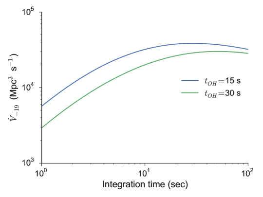
Figure 1: Dependence of $\dot{V}_{-19}$ on $t_{\rm exp}$ for ZTF (Bellm, 2014) for fiducial $t_{\rm OH}$ of 15 and 30 seconds. A longer overhead both decreases the maximum survey speed achievable and lengthens the optimum exposure time.

For definiteness, we use a fiducial value of $M=-19$ (characteristic of Type Ia supernovae) throughout this work. This choice creates some dependence on cosmology and assumed $k$-correction on the derived value of $\dot{V}_{M}$ for the deepest surveys. We use a cosmology with $h=0.704$, $\Omega_{m}=0.272$, $\Omega_{\Lambda}=0.728$ (Komatsu et al., 2011) as implemented in the package cosmolopy.

The total spatial volume surveyed in a cadence interval (a “snapshot”) is proportional to the number of transients in the snapshot. The figure of merit $\dot{V}_{M}$ thus describes the capability of a given observing system to trade the volume surveyed against revisit time. Maximizing $\dot{V}_{M}$ when designing a camera thus maximizes its ability to discover transients at any desired revisit time, subject to the constraints on cadence intervals that we will discuss in Section 3.

Not all transients are created equal, however. Full scientific exploitation of a detected transient typically requires additional photometric and spectroscopic followup. The feasibility of this followup depends strongly on the apparent magnitude of the transient. A survey discovering a smaller absolute number of transients may thus be more productive if those transients are brighter and can be observed with more readily available moderate-aperture followup telescopes.

Accordingly, we define a modified figure of merit, the spectroscopically-accessible volumetric survey speed:

$$\dot{V}_{M,m<s}=f_{\rm spec}(s)\dot{V}_{M},$$ (4)

where $f_{\rm spec}(s)$ is the fraction of the comoving volume producing transients with apparent magnitudes brighter than $s$. We choose $s$ based on the capability of the followup resources available: $s\approx 21$ is a reasonable limit for observations with 3–5 m telescopes, while $s\approx 23$ is reasonable for 8–10 m followup.

This scheme of defining $f_{\rm spec}$ with a sharp cutoff at apparent magnitude $s$ assumes our priority is to be capable of following up the faintest (presumably rare) transients. If instead we wish to obtain a large sample of transient spectra, it will be more useful to weight the comoving volume integral by the cost (in time) of followup as a function of apparent magnitude. This weighting will further emphasize the strengths of the wide, shallow surveys producing the most bright transients.

Because the sharp cutoff at apparent magnitude $s$ is conceptually simpler, we use it through the remainder of this work. We use $5\sigma$ limiting magnitudes throughout.

Table 1 lists instrument specifications and the resulting survey speeds for several major time-domain surveys. Figure 2 shows the impact of the limiting magnitude cut on $\dot{V}_{M}$ and on the optimal exposure time. Figure 3 shows the spatial volume surveyed as a function of transient brightness.

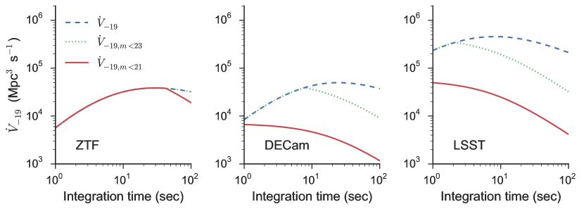
Figure 2: Variation in spectroscopically-accessible survey speed with exposure time for ZTF, DECam, and LSST. Solid red lines show the volume probed for transients brighter than 21^st mag ($\dot{V}_{-19,m<21}$), dotted green lines show $\dot{V}_{-19,m<23}$, and dashed blue lines show the total volumetric survey speed ($\dot{V}_{-19}$). Larger aperture telescopes may be less efficient at detecting bright transients even at short exposure times.

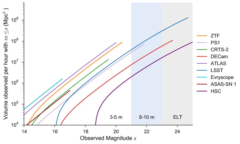
Figure 3: Spatial volume within which transients of absolute magnitude $-19$ may be detected in a one-hour survey snapshot versus the maximum apparent magnitude $s$ of the detection. Shaded regions indicate the telescope aperture necessary for spectroscopic followup.

Survey	$D$	$\Omega_{\rm fov}$	Etendue	Pixels	$t_{\rm exp}$	$t_{\rm OH}$	$m_{\rm lim}$	$\dot{\Omega}$	$N_{\rm obs}$	$\dot{V}_{-19}$	$f_{\rm spec}$
Camera	(m)	(deg2)	(m2 deg2)	(′′)	(sec)	(sec)		(deg2 hr-1)	(yr-1)	(Mpc3/s)
Evryscope	0.06(27$\times$)	8660	26.5	13.3	120	4	16.4	251419	19279	$1.1\text{\times}{10}^{04}$	1.00
ASAS-SN 1	0.14(4$\times$)	73	1.1	7.8	180	23	17	1294	99	$1.2\text{\times}{10}^{02}$	1.00
ATLAS	0.5(2$\times$)	60	11.8	1.9	30	8	20.0	5684	435	$2.3\text{\times}{10}^{04}$	1.00
CRTS	0.7	8.0	3.1	2.5	30	18	19.5	600	46	$1.4\text{\times}{10}^{03}$	1.00
CRTS-2	0.7	19.0	7.3	1.5	30	12	19.5	1628	124	$3.7\text{\times}{10}^{03}$	1.00
LSQ	1.0	8.7	6.8	0.9	60	40	20.5	313	24	$2.3\text{\times}{10}^{03}$	1.00
PTF	1.2	7.3	8.2	1.0	60	46	20.7	246	18	$2.3\text{\times}{10}^{03}$	1.00
Skymapper	1.3	5.7	7.5	0.5	110	20	21.6	157	12	$3.9\text{\times}{10}^{03}$	0.52
PS1 3$\pi$	1.8	7.0	17.8	0.3	30	10	21.8	630	48	$1.9\text{\times}{10}^{04}$	0.42
SST	2.9	6.0	39.6	0.9	1	6	20.7	3085	236	$2.7\text{\times}{10}^{04}$	1.00
MegaCam	3.6	1.0	10.2	0.2	300	40	22.8	10	0.8	$8.8\text{\times}{10}^{02}$	0.16
DECam	4.0	3.0	37.7	0.3	50	20	23.7	154	11	$2.9\text{\times}{10}^{04}$	0.07
HSC	8.2	1.7	89.8	0.2	60	20	24.6	76	5	$3.1\text{\times}{10}^{04}$	0.03
BlackGEM∗	0.6(4$\times$)	2(4$\times$)	11.3	0.6	30	5	20.7	822	63	$7.6\text{\times}{10}^{03}$	1.00
ZTF∗	1.2	47	53.1	1.0	30	15	20.4	3760	288	$2.5\text{\times}{10}^{04}$	1.00
LSST∗	6.7	9.6	319.5	0.2	30	11	24.7	842	64	$3.7\text{\times}{10}^{05}$	0.03

Table 1: Comparison of existing and planned wide-field optical survey cameras. For each camera we list telescope aperture ($D$), single-image field of view ($\Omega_{\rm fov}$), etendue, pixel scale, integration time ($t_{\rm exp}$), overhead per exposure ($t_{\rm OH}$), the $5\sigma$ single-exposure limiting magnitude in $r$ ($m_{\rm lim}$), the areal survey rate ($\dot{\Omega}$), the number of observations per field per year in a hypothetical uniform $3\pi$ survey averaging 6.5 hours per night observing time ($N_{\rm obs}$), the volume probed per unit exposure time for transients of absolute magnitude $-19$ ($\dot{V}_{-19}$), and the fraction of $\dot{V}_{-19}$ that is “spectroscopically accessible” ($m\leq 21$ mag; $f_{\rm spec}\equiv\dot{V}_{-19,m<21}/\dot{V}_{-19}$) Performance for future (^∗) surveys is estimated. BlackGEM values are for Phase 1 (4 telescopes); ASAS-SN values are for a single site. CRTS values are for the CSS telescope only. SST and LSST diameters are effective apertures. References: Evryscope: Law et al. (2015); ASAS-SN: Shappee et al. (2014), B. Shappee, priv. comm.; ATLAS: Tonry (2011, 2013), J. Tonry priv. comm.; CRTS: Drake et al. (2009); CRTS-2: A. Mahabal, priv. comm.; LSQ (La Silla QUEST): Rabinowitz et al. (2012); PTF: Law et al. (2009); Skymapper: Keller et al. (2007); PS1: Kaiser (2004), Morganson et al. (2012); SST: Freedman Woods et al. (2014), Ruprecht et al. (2014); MegaCam: Boulade et al. (2003), http://www.cfht.hawaii.edu/Instruments/Imaging/MegaPrime/quickinformation.html; DECam: DePoy et al. (2008), NOAO Data Handbook; HSC: Miyazaki et al. (2012), Tanaka et al. (2016), HSC E.T.C.; BlackGEM: http://astro.ru.nl/blackgem/; ZTF: Bellm (2014); LSST: LSST Science Collaboration (2009).

3 Cadence

In Section 2, we showed the effectiveness of wide, shallow surveys in detecting spectroscopically-accessible transients. However, the proportionality between $\dot{V}_{M}$ and the number of detected transients breaks down if a survey runs out of new sky to observe. For modern wide-field surveys, it is easily feasible to observe the entire visible sky in less than one night. We therefore must consider the relationship between a survey’s areal survey speed $\dot{\Omega}=\frac{\Omega_{\rm fov}}{t_{\rm exp}+t_{\rm OH}}$, its latitude $\phi$, and the possible cadences.

In this section, we consider an idealized and simplified transient survey. We assume that our survey operates in a single filter bandpass at a single site with no weather losses. While observing, we observe the largest snapshot area ($\Omega_{\rm snap}$) possible in the cadence interval ($\Delta t$) such that we can observe the entire footprint a second time in the second epoch. We assume a single exposure time (optimized for the cadence interval chosen if necessary) and a fixed overhead between exposures, implying roughly constant slews between each exposure. Finally, we limit our observations in the footprint to times when the fields are above a specified maximum airmass or zenith angle ($\zeta_{\rm max}$).

The trade space between survey snapshot area $\Omega_{\rm snap}$ and cadence interval $\Delta t$ has two limits. The first is when an instrument sits on a single field and takes exposures at a rate limited only by its readout time. In this case $\Omega_{\rm snap,min}=\Omega_{\rm fov}$ and $\Delta t_{\rm min}=t_{\rm OH}$. Surveys operating at this limit are usually driven by specialized science goals; they are best undertaken by instruments with extremely large fields of view (such as Pi of the Sky (Burd et al., 2005) or Evryscope (Law et al., 2014)) and/or fast readout time (EM-CCDs or CMOS).

The opposite limit is to maximize the snapshot volume, and hence use the longest cadence interval possible. The maximum revisit time ($\Delta t_{\rm max}$) is set by how long it takes a survey with areal survey speed $\dot{\Omega}$ to cover the entire visible sky area. The limit of the “available sky” thus depends on the observatory latitude, which determines the length of the night as well as the rotation rate of new sky into the observable region above $\zeta_{\rm max}$.

Calculating the limiting cadence interval $\Delta t_{\rm max}$ requires consideration of several cases. The sky area above the zenith angle cut $\zeta_{\rm max}$ at any given instant may be divided into a circumpolar region and a region that will rotate below $\zeta_{\rm max}$ eventually:

$$\Omega_{\rm inst}=\Omega_{\rm circ}+\Omega_{\rm r}=2\pi(1-\cos\zeta_{\rm max}).$$

(Depending on the latitude and $\zeta_{\rm max}$, there may be no circumpolar region or the entire sky may be circumpolar.) Since the circumpolar region stays above the zenith angle cut, the rate of change of this instantaneous sky is

$$\frac{d\Omega_{\rm inst}}{dt}=\frac{d\Omega_{\rm r}}{dt}$$

The rotation of sky into and out of $\Omega_{\rm r}$ is most easily calculated by integrating the areal rotation across the meridian. The total sky area passing above $\zeta_{\rm max}$ in one night is therefore

$$\Omega_{\rm night}=\Omega_{\rm inst}+\frac{d\Omega_{\rm r}}{dt}\Delta t_{\rm night}.$$

Figure 4 shows the dependence of the total sky available per night on observatory latitude.

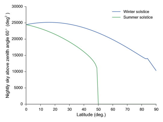
Figure 4: Unique sky area per night above $\zeta_{\rm max}=60^{\circ}$ as a function of observatory latitude. Night lengths are determined for 18^∘ twilight, and the limiting values at the summer and winter solstices are shown. The cusp near 84^∘ latitude is due to the transition to 24 hrs of $>18^{\circ}$ darkness.

The first case of limiting cadences to consider is for instruments capable of surveying the entire sky in less than a single night. These must have areal survey rates $\dot{\Omega}>\frac{d\Omega_{\rm r}}{dt}$: they must be able to survey the sky in the region above $\zeta_{\rm max}$ faster than it rotates out of the available field. In this case $\Omega_{\rm snap}=\Omega_{\rm inst}$: we choose a footprint such that at the end of the first epoch, the trailing edge has risen to $\zeta_{\rm max}$ to be observed and the leading edge of the footprint has just rotated down to $\zeta_{\rm max}$ to be observed in the second epoch. The limiting cadence interval is thus $\Delta t_{\rm max}=\Omega_{\rm inst}/\dot{\Omega}$. The remaining check is to ensure that $\Delta t_{\rm max}$ is less than half of the night length.

In cases where $\dot{\Omega}<\frac{d\Omega_{\rm r}}{dt}$ or it takes longer than half a night to survey $\Omega_{\rm inst}$, it will take more than one night to repeat observations of the available sky above $\zeta_{\rm max}$. For instruments with $\dot{\Omega}$ greater than $\frac{d\Omega_{\rm r}}{dt}$ scaled to the nightly sidereal rotation, the argument is identical to the sub-night case. We replace $\Omega_{\rm inst}$ by $\Omega_{\rm night}$ averaged over the cadence interval and restrict the observing time within $\Delta t$ to the times the sun is down. Given the dependence on night length, $\Omega_{\rm snap,max}$ and $\Delta t_{\rm max}$ are most conveniently found numerically.

Instruments with $\dot{\Omega}$ slower than the sidereal rotation of the footprint are unlikely to be used for time domain surveys, so we do not consider them further.

Figure 5 plots the areal survey speeds of several cameras against the footprint rotation rate $\frac{d\Omega_{\rm r}}{dt}$.

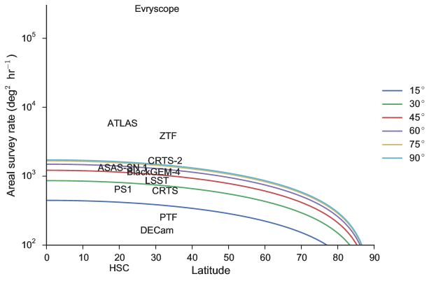
Figure 5: Areal survey rates ($\dot{\Omega}$, in deg² hr^-1) for specific surveys. Overplot colored lines are the rate of change of sky area above a given zenith angle cut $\zeta_{\rm max}$ as a function of latitude ($\frac{d\Omega_{\rm r}}{dt}$, in deg² hr^-1). Surveys above a given line can survey faster than the sky rotates within the footprint defined by $\zeta_{\rm max}$.

Figures 6 and 7 plot the snapshot volume against the cadence interval, with and without a cutoff on the transient limiting magnitude.

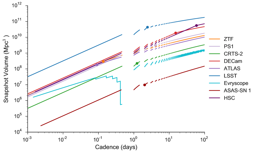
Figure 6: Total snapshot survey volume for $M=-19$ transients versus cadence interval for several surveys. Observations begin on the winter solstice. Filled circles indicate the cadence interval at which the survey runs out of available sky above an airmass of 2.5. Below this point the snapshot volume is simply the survey speed $\dot{V}_{M}$ times the available observing time. Above this point we increase the exposure time to reach longer cadence intervals, at cost of a slower rate of increase in the snapshot volume.

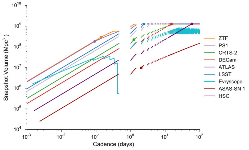
Figure 7: Same as Figure 6, but for spectroscopically-accessible volume only ($\dot{V}_{M,m<21}$): we consider only the volume in which we can detect transients of apparent magnitude brighter than $m=21$, appropriate for 3–5 m-class spectroscopic followup. ZTF and ATLAS will discover more bright transients at any chosen cadence interval than even LSST.

For some cameras, the longest sky-limited cadence interval $\Delta t_{\rm max}$ may be shorter than the transient timescale of interest. For example, superluminous supernovae (SLSN) may be visible for hundreds of days; two all-sky surveys with identical depths using a one day and a one week cadence would thus each discover SLSN at the same rate. Several modifications of our baseline survey are possible in this case. A first option is to maintain the higher cadence, achieving finer sampling of the lightcurve and hence improved characterization of the lightcurve shape. This may be scientifically valuable in many cases, although it does not increase the transient detection rate. A second option is to integrate for longer exposures than needed to maximize $\dot{V}_{M}$, as in the sky-limited case the “optimal” exposure time no longer maximizes the number of detected transients. However, with deeper exposures the additional transients discovered will be more challenging to follow up. Survey extensions are also possible: surveys in other filters or of other programs can productively fill time before beginning a new epoch.

4 Detection

The selection of a specific cadence interval $\Delta t$ sets the volume $V_{\rm snap}(M)$ within which transients of absolute magnitude $M$ may be detected. It also imposes a selection effect on the decay timescale of the transients detected. In particular, events which decay much more quickly than $\Delta t$ are unlikely to be detected.

Exact computation of detection rates requires detailed modeling of multi-color lightcurves, detection passbands, cosmological evolution of event rates, event-to-event variations, and more (e.g., Kessler et al., 2009). Our goal in this work is to provide a reasonable comparison of survey camera capability and broad cadence tradeoffs rather than a precise estimate of the rates of specific event types. Accordingly, we make several simplifying assumptions to enable analytic integrals. However, it is straightforward to extend this methodology to specific event classes by substituting appropriate lightcurve shapes, k-corrections, evolution of the rates with redshift, and extinction.

We calculate the yearly detection rate for transients of absolute magnitude $M$ and rest-frame effective decay timescale $\tau_{\rm eff}$ by integrating over the co-moving volume:

$$N(M,\tau_{\rm eff},m_{\rm lim},\Delta t)=\Omega_{\rm snap}\int_{0}^{z_{\rm lim}(M,m_{\rm lim})}\!\frac{\mathcal{R}(z)}{1+z}ct_{k}(M,m_{\rm lim},\tau_{\rm eff},z)\frac{dV}{dz}dz.$$ (5)

Here $\mathcal{R}(z)$ is the comoving volumetric rate (events Mpc^-3 yr^-1); we divide by (1+$z$) due to time dilation. The survey limiting magnitude determines the depth of the spatial cone probed, while the choice of cadence interval $\Delta t$ determines its angular extent $\Omega_{\rm snap}$.

We calculate the effect of observing cadence on the discovery rate using the control time $ct_{k}$. Here $k$ is the number of consecutive images in which we require a detection. If a given transient is detectable in the observer frame above $m_{\rm lim}$ for time $t_{\rm vis}$, given an array of separations $dt_{i}$ between $n$ consecutive images of a field, we define $r$ as the number of intervals where $dt_{i}<t_{\rm vis}$. Then the control time is defined by Zwicky (1942) as

$$ct_{1}(t_{\rm vis})=\sum_{1}^{r}dt_{i}+(n-r)t_{\rm vis}.$$ (6)

Using the control time in this manner counts even a single detection of an event above the limiting magnitude towards the total number of events discovered ($k=1$). In modern transient surveys it is common to require multiple detections of an event before triggering followup in order to avoid contamination by uncatalogued asteroids and image subtraction artifacts. We develop here an extension of the $ct_{1}$ algorithm for $k>1$ (Algorithm 1).

Algorithm 1 Algorithm for computing the control time $ct_{k}$ from $n$ observations with timestamps $t_{i}$, requiring $k>1$ consecutive observations within the visibility interval $t_{\rm vis}$.

begin

for $j:=0$ to $n-k$ do

     begin

     $dt_{j}=t_{j+k-1}-t_{j}$

     if $dt_{j}>t_{\rm vis}$ then

         $ct_{j}=0$

     else

         if $ct_{j-1}=0{~{}\rm\bf or~{}}j=0$ then

              $ct_{j}=t_{\rm vis}$

         else

              $ct_{j}=dt_{j}$

     end

$ct_{k}=\sum_{j=0}^{n-k}ct_{j}$

end.

We use a simple analytic approximation for the lightcurve shape to simplify the calculation of the control time. We assume that the transient rises and falls linearly in magnitude space with characteristic rest-frame timescales $\tau_{\rm rise}$ and $\tau_{\rm fall}$ days mag^-1. Accordingly, the source is visible in the observer frame for

$$t_{\rm vis}(M,m_{\rm lim},\tau_{\rm rise},\tau_{\rm fall}) =((M-m_{\rm lim})\tau_{\rm rise}+(M-m_{\rm lim})\tau_{\rm fall})(1+z)$$ (7)

$$\equiv(M-m_{\rm lim})\tau_{\rm eff}(1+z).$$ (8)

For many explosive transients, $\tau_{\rm fall}>>\tau_{\rm rise}$, so $\tau_{\rm eff}\approx\tau_{\rm fall}$.

Using these assumptions, we may now compute (idealized) detection rates for different surveys and cadences. We calculate the detection rates in a grid of transient peak magnitude $M$ and effective timescale $\tau_{\rm eff}$ (cf. Kasliwal, 2011). We use a constant fiducial volumetric rate density $\mathcal{R}(z)=3\times 10^{-5}$ events Mpc^-3 yr^-1, approximately the local SN Ia rate. As above, we use the k-correction of a hypothetical $f_{\lambda}$ standard.

For each cadence interval $\Delta t$, we create a grid of times for a one-year interval with spacing $\Delta t$. We mask all grid points between eighteen degree dawn and eighteen degree twilight and use the remainder as our observation times $t_{i}$ to compute the control time. As discussed in Section 3, when the desired cadence interval is longer than the time needed to survey the available sky above an airmass of 2.5 we increase the exposure time to compensate (cf. Figure 6).

Figure 8 shows the detection rate for PTF using a 1 day cadence in the phase space of transient peak magnitude and effective timescale. Comparing the predicted numbers of detections at timescales less than a day to the paucity of fast transients discovered to date (cf. LSST Science Collaboration, 2009; Kasliwal, 2011) emphasizes that any fast transients that exist must be rare, as current surveys already have some sensitivity to short-timescale events. We also could easily invert the calculation to determine the volumetric rate $\mathcal{R}(z)$ compatible with current nondetections.

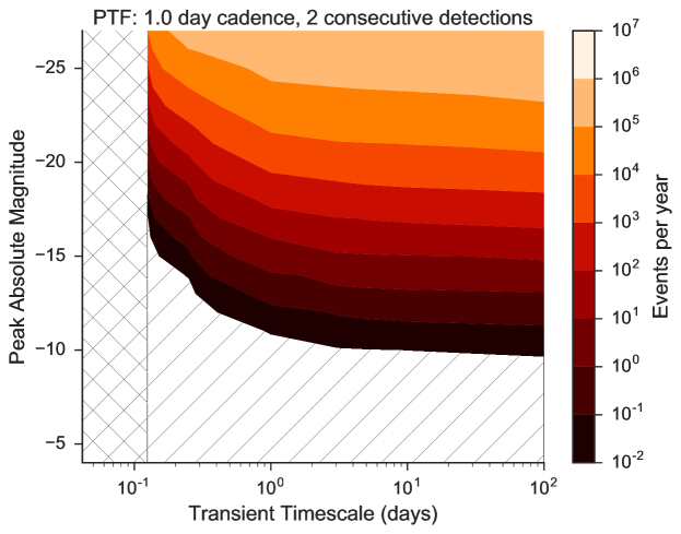
Figure 8: Number of transients detectable in at least two epochs by PTF using a strict 1 day cadence with no weather losses as a function of peak absolute magnitude and effective timescale $\tau_{\rm eff}$. Colors indicate the number of events detected per year assuming all transients occur at the local SN Ia rate. Transients in the hashed region are detected at a rate of less than one per century, while events in the crosshatched region cannot be detected twice by the specified cadence.

In Figure 9, we slice Figure 8 at the fiducial value of $M=-19$ mag and compare PTF 1 day and 1 hour cadences to ZTF at a 1 hour cadence. By increasing the raw survey speed relative to PTF, ZTF can break from the cadence–survey volume trade space defined by PTF and conduct a survey that is both wide area and high cadence. Such a survey is required to discover intrinsically rare, fast-decaying events such as gamma-ray burst afterglows.

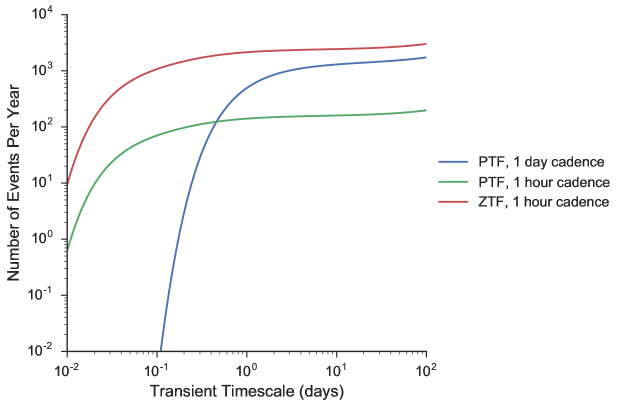
Figure 9: Comparison of the number of $M=-19$ transients detectable by PTF and ZTF as a function of cadence interval and effective timescale $\tau_{\rm eff}$. The requirement to detect the transient in at least two epochs leads to a sharp drop in the number of events detected below the cadence interval $\Delta t$. PTF can increase its sensitivity to (intrinsically rare) fast transients by observing at a 1 hour cadence rather 1 day cadence, but this decreases the number of slow transients it detects by an order of magnitude. Thanks to its much greater survey speed $\dot{V}_{-19}$, ZTF can discover more transients than PTF at all timescales $\tau_{\rm eff}$ even with a 1 hour cadence.

With the ability to estimate the transient detection rate as a function of cadence, it is then possible to choose a cadence interval to optimize the total number of detections for one or several source classes. Figures 10 and 11 show the dependence of the detection rate on the chosen survey cadence for decay rates $\tau_{\rm eff}=20$ and 1 days mag^-1.

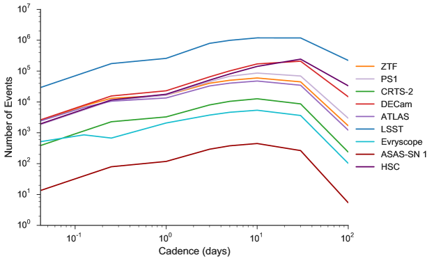
Figure 10: Number of $M=-19,\tau_{\rm eff}=20$ days mag^-1 transients detected in at least two epochs by various surveys as a function of cadence interval, assuming a constant volumetric rate equal to the local SN Ia rate. At short cadences ($\Delta t<<\tau_{\rm eff}$), high $\dot{\Omega}$ surveys like ZTF and ATLAS can discover comparable numbers of transients to deeper surveys like DECam and HSC. At long cadences ($\Delta t>>\tau_{\rm eff}$), the detection efficiency of all surveys declines because all but the brightest nearby events decay too quickly to be observed in a second epoch.

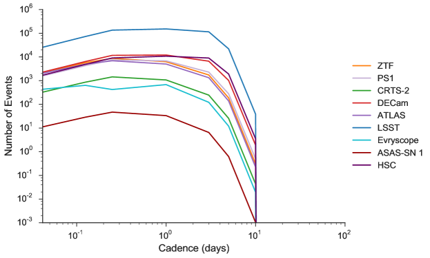
Figure 11: Number of $M=-19,\tau_{\rm eff}=1$ day mag^-1 transients detected in at least two epochs by various surveys.

5 Conclusion

To obtain useful comparisons of transient surveys, it is necessary to look beyond simple calculations of étendue. We have developed a new means of comparing current and near-term time-domain surveys: the instantaneous volumetric survey speed. This metric requires only readily-available information: the camera field of view, exposure and overhead times, and limiting magnitude. It captures the relationship between the cadence interval and the survey snapshot volume, which is related to the discovery rate. The volumetric survey speed is straightforward to interpret physically, and additionally it implies an optimal integration time.

A closely-related metric is the areal survey rate, which serves to bound the achievable cadences for a ground-based survey. Simply put, many modern time-domain surveys run out of fresh sky to survey, sometimes in a single night! Another practical concern is the brightness of the discovered transients—for science applications requiring spectroscopic followup, discovering many faint transients is often less valuable than a finding a few bright ones.

We have developed a basic analytic framework for estimating the detection rate of transients that evolve at different speeds. By assessing the influence of the survey parameters and the chosen survey cadence on the detection rate, one may optimize the survey cadence for the science of interest and compare to other surveys. A complete evaluation of detection rates for specific transient types will require analysis of actual simulated or realized pointing histories, with increased fidelity coming at the cost of additional complexity. LSST’s Metrics Analysis Framework (Jones et al., 2014) provides one such means of performing quantitative assessments of pointing histories.

Maximizing the transient detection rate does not alone optimize a survey design. In many cases, there is tension between the need for well-sampled transient lightcurves and the desire to maximize the discovery rate. Practical limits such as the availability of followup resources, theoretical or systematic limitations, or multiple scientific objectives may also apply. However, quantitative assessment of these tradeoffs and of the competitive landscape will strengthen the design of transient surveys.

References

- Bellm (2014) Bellm, E. 2014, in The Third Hot-wiring the Transient Universe Workshop, ed. P. R. Wozniak, M. J. Graham, A. A. Mahabal, & R. Seaman, 27
- Boulade et al. (2003) Boulade, O., Charlot, X., Abbon, P., et al. 2003, in Proc. SPIE, Vol. 4841, Instrument Design and Performance for Optical/Infrared Ground-based Telescopes, ed. M. Iye & A. F. M. Moorwood, 72
- Burd et al. (2005) Burd, A., Cwiok, M., Czyrkowski, H., et al. 2005, New A, 10, 409
- DePoy et al. (2008) DePoy, D. L., Abbott, T., Annis, J., et al. 2008, in Proc. SPIE, Vol. 7014, Ground-based and Airborne Instrumentation for Astronomy II, 70140E
- Drake et al. (2009) Drake, A. J., Djorgovski, S. G., Mahabal, A., et al. 2009, ApJ, 696, 870
- Freedman Woods et al. (2014) Freedman Woods, D., Lambour, R. L., Faccenda, W. J., et al. 2014, in Society of Photo-Optical Instrumentation Engineers (SPIE) Conference Series, Vol. 9149, Observatory Operations: Strategies, Processes, and Systems V, 91490S
- Hogg (1999) Hogg, D. W. 1999, ArXiv Astrophysics e-prints, astro-ph/9905116
- Jones et al. (2014) Jones, R. L., Yoachim, P., Chandrasekharan, S., et al. 2014, in Society of Photo-Optical Instrumentation Engineers (SPIE) Conference Series, Vol. 9149, Observatory Operations: Strategies, Processes, and Systems V, 91490B
- Kaiser (2004) Kaiser, N. 2004, in Society of Photo-Optical Instrumentation Engineers (SPIE) Conference Series, Vol. 5489, Society of Photo-Optical Instrumentation Engineers (SPIE) Conference Series, ed. J. M. Oschmann, Jr., 11
- Kasliwal (2011) Kasliwal, M. M. 2011, PhD thesis, California Institute of Technology
- Keller et al. (2007) Keller, S. C., Schmidt, B. P., Bessell, M. S., et al. 2007, PASA, 24, 1
- Kessler et al. (2009) Kessler, R., Bernstein, J. P., Cinabro, D., et al. 2009, PASP, 121, 1028
- Komatsu et al. (2011) Komatsu, E., Smith, K. M., Dunkley, J., et al. 2011, ApJS, 192, 18
- Law et al. (2014) Law, N. M., Fors, O., Wulfken, P., Ratzloff, J., & Kavanaugh, D. 2014, in Society of Photo-Optical Instrumentation Engineers (SPIE) Conference Series, Vol. 9145, Society of Photo-Optical Instrumentation Engineers (SPIE) Conference Series, 0
- Law et al. (2009) Law, N. M., Kulkarni, S. R., Dekany, R. G., et al. 2009, PASP, 121, 1395
- Law et al. (2015) Law, N. M., Fors, O., Ratzloff, J., et al. 2015, PASP, 127, 234
- LSST Science Collaboration (2009) LSST Science Collaboration. 2009, ArXiv e-prints, arXiv:0912.0201 [astro-ph.IM]
- Miyazaki et al. (2012) Miyazaki, S., Komiyama, Y., Nakaya, H., et al. 2012, in Proc. SPIE, Vol. 8446, Ground-based and Airborne Instrumentation for Astronomy IV, 84460Z
- Morganson et al. (2012) Morganson, E., De Rosa, G., Decarli, R., et al. 2012, AJ, 143, 142
- Rabinowitz et al. (2012) Rabinowitz, D., Schwamb, M. E., Hadjiyska, E., & Tourtellotte, S. 2012, AJ, 144, 140
- Ruprecht et al. (2014) Ruprecht, J. D., Stuart, J. S., Woods, D. F., & Shah, R. Y. 2014, Icarus, 239, 253
- Shappee et al. (2014) Shappee, B. J., Prieto, J. L., Grupe, D., et al. 2014, ApJ, 788, 48
- Tanaka et al. (2016) Tanaka, M., Tominaga, N., Morokuma, T., et al. 2016, ArXiv e-prints, arXiv:1601.03261 [astro-ph.HE]
- Terebizh (2011) Terebizh, V. Y. 2011, Astronomische Nachrichten, 332, 714
- Tonry (2011) Tonry, J. L. 2011, PASP, 123, 58
- Tonry (2013) —. 2013, Royal Society of London Philosophical Transactions Series A, 371, 20269
- Zwicky (1942) Zwicky, F. 1942, ApJ, 96, 28