The Goodness of Simultaneous Fits in ISIS

Abstract

In a previous work, we introduced a tool for analyzing multiple datasets simultaneously, which has been implemented into ISIS. This tool was used to fit many spectra of X-ray binaries. However, the large number of degrees of freedom and individual datasets raise an issue about a good measure for a simultaneous fit quality.

We present three ways to check the goodness of these fits: we investigate the goodness of each fit in all datasets, we define a combined goodness exploiting the logical structure of a simultaneous fit, and we stack the fit residuals of all datasets to detect weak features. These tools are applied to all RXTE-spectra from GRO 1008$-$57, revealing calibration features that are not detected significantly in any single spectrum. Stacking the residuals from the best-fit model for the Vela X-1 and XTE J1859+083 data evidences fluorescent emission lines that would have gone undetected otherwise.

1 Introduction

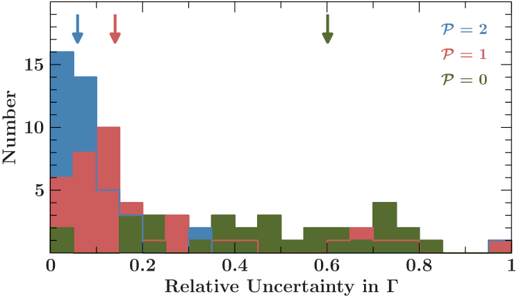
Figure 1: Distribution of the relative uncertainties (90% confidence level) of the power-law photon indices, $\Gamma$, in our study of all RXTE-observations of GRO J1008$-$57 [7]. Fitting all 43 observations separately results in the green histogram. As soon as we perform a simultaneous fit with $\mathcal{P}=1$ global continuum parameter the uncertainties decrease significantly as shown by the red histogram. Finally, using $\mathcal{P}=2$ global parameters (blue histogram) results in a median of ${\sim}6\%$ in the uncertainties (compare the arrows on top).

Nowadays, the still increasing computation speed and available memory allows us to analyze large datasets at the same time. Using X-ray spectra of accreting neutron stars as an example, we have shown in a previous paper [1, hereafter paper I] that loading and fitting the spectra simultaneously has several advantages compared to the “classical” way of X-ray data analysis, which is treating every observation individually. In particular, instead of fixing parameters to a mean value one can determine them by a joint fit to all datasets under consideration. Due to the reduced number of degrees of freedom the remaining parameters can be better constrained (see Fig. 1 as an example). Furthermore, parameters no longer need to be independent, but can be combined into functions. For instance, the slope of the spectra might be described as a function of flux with the coefficients of this function as fit-parameters.

The disadvantages of fitting many datasets simultaneously are, however, an increased runtime and a complex handling because of the large number of parameters. In paper I, we have introduced functions to facilitate this handling, which have been implemented into the Interactive Spectral Interpretation System (ISIS) [2]. While these functions are already available as part of the ISISscripts they are continuously updated and new features are implemented. One important question, which we raised in paper I, is about the goodness of a simultaneous fit as it is, e.g., calculated after the commonly used $\chi^{2}$-statistics, particularly the case where some datasets are not described well by the chosen model. Due to the potential large total number of datasets, the information about failed fits can be hidden in the applied fit-statistics. After we have given a reminder about the terminology of simultaneous fits in Section 1.1, we describe the problem of detecting failed fits in more detail in Section 2 and provide possible solutions. We will conclude this paper by applying these solutions to examples in Section 3.

1.1 Simultaneous Fits

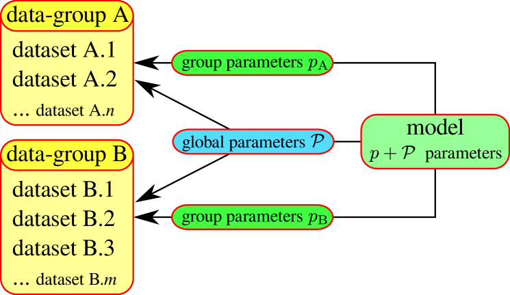
Figure 2: Terminology of simultaneous fits in ISIS, according to paper I. A data-group consists of simultaneously taken datasets, here data-group A has $n$ and B has $m$ datasets. A model with $p+\mathcal{P}$ parameters is fitted such that each data-group has its own set of $p_{i}$ parameters, called group parameters. The common $\mathcal{P}$ parameters between the groups are the so-called global parameters.

As we have described in paper I, a data-group contains all datasets which have been taken simultaneously in time or, in general, represent the same state of the observed object. In the example illustrated in Fig. 2 two data-groups, A and B, have been added to the simultaneous fit, containing $n$ and $m$ datasets, respectively. Thus, a dataset is labeled by the data-group it belongs to, e.g., B3 is the third dataset in the second data-group. After a model with $p$ parameters has been defined each of these data-groups is fitted by an individual set of parameters, called group parameters. Consequently, all datasets belonging to a specific data-group are described by the same parameter values. A specific group parameter can now be marked as a so-called global parameter. The value of the corresponding group parameters will now be tied to this global parameter, i.e, this parameter has a common value among all data-groups. Instead of tying group parameters together to a global value, a parameter function may be defined, to which the group parameters are set instead. This function takes, e.g., other parameters as input to calculate the value for each group parameter. In this case, correlations between model parameters, e.g, as predicted by theory can be implemented and fitted directly.

2 Goodness of a simultaneous fit

As an indicator for the goodness of a fit the analysis software used, e.g ISIS or XSPEC [3], usually displays the fit-statistics after the model has been fitted to the data. Here, we chose the $\chi^{2}$-statistics since the developed functions for a simultaneous fit have been first applied to accreting neutron stars. The high count rates satisfies the Gaussian approxmation of the uncertainties, which are actually Poisson distributed. In principle, however, the discussed issues and their solutions can be generalized for any kind of fit-statistics.

For each datapoint $k$ the difference between the $\mathrm{data}$ and the $\mathrm{model}$ is calculated and normalized by the measurement uncertainty, $\mathrm{error}$, of the data. The sum over all $n$ datapoints is called the $\chi$-square,

$$\chi^{2}=\sum_{k=1}^{n}\frac{(\mathrm{data}_{k}-\mathrm{model}_{k})^{2}}{\mathrm{error}_{k}^{2}}$$ (1)

and is displayed after a fit. Additionally, the sum is normalized to the total number of degrees of freedom, $n-p$ with the number of free fit-parameters $p$, since the $\chi^{2}$ increases with $n$. This normalized sum, called the reduced $\chi$-square,

$$\chi^{2}_{\mathrm{red}}=\frac{\chi^{2}}{n-p}$$ (2)

is also displayed. For Gaussian distributed data the expected value is $\chi^{2}_{\mathrm{red}}=1$ for a perfect fit of the chosen model. However, once the probability distribution is changed, e.g., when a spectrum has been rebinned, the expected value changes as well. Consequently, a reliable measure for the goodness of the fit has to be defined with some forethought.

The $\chi^{2}_{\mathrm{red}}$ threshold, for which a simultaneous fit is acceptable, strongly depends on the considered case. In particular, a few data-groups might not be described well by the chosen model, which would result in an unacceptable $\chi^{2}_{\mathrm{red}}$ when fitted individually. However, in case of a simultaneous fit, this information might be hidden in the classical definition of the $\chi^{2}_{\mathrm{red}}$ (Eq. 2). Let us consider $N$ data-groups and a model with $p$ group parameters and $\mathcal{P}$ global parameters. Then, the total $\chi^{2}_{\mathrm{red}}$ is

$$\chi^{2}_{\mathrm{red}}=\frac{\sum_{i=1}^{N}\chi^{2}_{i}}{\sum_{i=1}^{N}(n_{i}-p_{i})-\mathcal{P}}$$ (3)

with the number of degrees of freedom, $n_{i}-p_{i}$, and the $\chi^{2}_{i}$ for each data-group $i$ after Eq. 1. Now, we assume a failed fit with $\chi^{2}_{i}\sim 2$ for a particular $i$ to be present, while for the remaining data-groups $\chi^{2}_{i}\sim 1$. For $N\gtrsim 10$ the $\chi^{2}_{\mathrm{red}}$ after Eq. 3 is still near unity and, thus, suggests a successful simultaneous fit. In the following, we present three possibilities to investigate the goodness of a simultaneous fit more carefully.

2.1 Histogram of the goodness

A trivial but effective solution is to check the goodness of the fit for each data-group individually. Here, in the chosen case of the $\chi^{2}$-statistics, the $\chi^{2}_{\mathrm{red,i}}$ is calculated for each data-group, $i$, after

$$\chi^{2}_{\mathrm{red,i}}=\frac{\chi^{2}_{i}}{n_{i}-p_{i}}$$ (4)

where $n_{i}$ are the number of datapoints in the data-group, and $p_{i}$ is the number of free group parameters. Due to that the global parameters are not taken into account here, the $\chi^{2}_{\mathrm{red,i}}$ is, however, different to that performed by a single fit of the data-group.

In the case of a large number of data-groups, it is more convenient to sort the $\chi^{2}_{\mathrm{red,i}}$ into a histogram to help investigating the goodness of the fit to all data-groups. We have added such a histogram to the simultaneous fit functions as part of the ISISscripts. After a fit has been performed using the fit-functions fit_groups or fit_global (see paper I) this histogram is added to the default output of the fit-statistics. In this way, failed fits of specific data-groups can be identified by the user at first glance.

2.2 A combined goodness of the fit

Instead of a few failed fits to certain data-groups, one might ask if the chosen model fails in the global context of a simultaneous fit. To answer this question, a special goodness of the simultaneous fit is needed to take its logical structure into account. As explained in Section 1.1, a data-group represents a certain state of the observed object, e.g., the datasets where taken at the same time. Thus, the data-groups are statistically independent of each other. Calculating the goodness of the fit in a traditional way, which is the $\chi^{2}_{\mathrm{red}}$ after Eq. 3 in our case, does not, however, take this aspect into account. As a solution we propose to define a combined goodness of the fit calculating the weighted mean of the individual goodness of each data-group. In the case of $\chi^{2}$-statistics, a combined reduced $\chi^{2}$ is calculated by

$$\chi^{2}_{\mathrm{red,comb.}}=\frac{1}{N}\sum_{i=1}^{N}\frac{\chi_{i}^{2}}{n_{i}-p_{i}-\mu_{i}\mathcal{P}}$$ (5)

with $\chi_{i}^{2}$ computed after Eq. 1 for each data-group, $i$, and a weighting factor, $\mu_{i}$, for the number of global parameters, $\mathcal{P}$:

$$\mu_{i}\approx(n_{i}-p_{i})\times\sum_{j=1}^{N}\frac{1}{n_{j}-p_{j}}$$ (6)

Thus, $\mu_{i}$ normalizes the effect of data-group $i$ on the determination of the global parameters, $\mathcal{P}$, by its number of degrees of freedom relative to the total number of degrees of freedom of the simultaneous fit. Equation 6 is, however, an approximation only. A data-group might not be sensitive to a certain global parameter, e.g, if the spectra in this data-group do not cover the energy range necessary to determine the parameter.

A failed fit to a specific data-group, for example with a high individual $\chi^{2}_{\mathrm{red,i}}$, has a higher impact on the $\chi^{2}_{\mathrm{red,comb.}}$ (Eq. 5) than on the traditional $\chi^{2}_{\mathrm{red}}$ (Eq. 2). In general we expect $\chi^{2}_{\mathrm{red,comb.}}\geq\chi^{2}_{\mathrm{red}}$, even if all data-groups are fitted well. In the case of a good simultaneous fit (better than a certain threshold), a weak feature in the data might still be unnoticed, if it is not detected in any individual data-group. Such a feature can be investigated by stacking the residuals, as outlined in the following section.

We note, however, that Eq. 5 is the result of an empirical study. A more sophisticated goodness of a simultaneous fit should be based on a different type of fit-statistics suitable for a simultaneous analysis of many datasets, such as a Bayesian approach or a joint likelihood formalism similar to anderson2015a [4].

2.3 Stacked residuals

Once datasets can be technically stacked to achieve a higher signal-to-noise ratio, e.g., when spectra have the same energy grid and channel binning, further weak features might get visible. This is a common technique in astrophysics [see, e.g., 5, 6]. However, when stacked datasets are analyzed, differences in the individual datasets, like source intrinsic variability, can no longer be revealed.

In case of a simultaneous fit, the residuals of all data-groups can be stacked instead. The stacking dramatically increases the total exposure in each channel bin. Thus, the stacked residuals of all data-groups, $R(k)$, as a function of the energy bin, $k$, can be investigated to further verify the goodness of the simultaneous fit

$$R(k)=\sum_{i=1}^{N}\mathrm{data}_{i,k}-\mathrm{model}_{i,k}$$ (7)

This task can be achieved using, e.g, the plot_data function written by M. A. Nowak.

We can show that the combined reduced $\chi^{2}$ is effectively equal to the goodness of a fit of the stacked data in the first place. Assuming the same number of degrees of freedom, $n-p$, for each data-group, Eq. 5 gives

$$\chi^{2}_{\mathrm{red,comb.}}=\frac{1}{f}\sum_{i=1}^{N}\sum_{k=1}^{n}\frac{(\mathrm{data}_{i,k}-\mathrm{model}_{i,k})^{2}}{\mathrm{error}_{i,k}^{2}}$$ (8)

with $f=N(n-p-\mu\mathcal{P})$ and having used Eq. 1. Now, the summand no longer depends on $i$ or $k$ explicitly. Thus, the order of the sums in Eq. 8 may be switched. If we finally interpret $k$ as a spectral energy bin we end up with the goodness as a function of $k$:

$$\begin{split}\chi^{2}_{\mathrm{red,comb.}}(k)&\propto\sum_{i=1}^{N}\frac{(\mathrm{data}_{i,k}-\mathrm{model}_{i,k})^{2}}{\mathrm{error}_{i,k}^{2}}\\ &\propto\sum_{i=1}^{N}\mathrm{data}_{i,k}^{2}\end{split}$$ (9)

This means that all datasets of the simultaneous fit are first summed up for each energy bin in the combined reduced $\chi^{2}$. In contrast to stacking the data in the first place, however, source variability can still be taken into account during a simultaneous fit.

Note that once all data-groups have the same number of degrees of freedom, the $\chi^{2}_{\mathrm{red,comb.}}$ (Eq. 8) is equal to the classical $\chi^{2}_{\mathrm{red}}$ (Eq. 2). To further investigate the goodness of the simultaneous fit in such a case, the histogram of the goodness of all data-groups (see Sec. 2.1) and, if possible, the stacked residuals should be investigated.

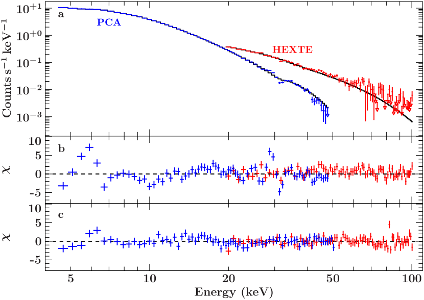
Figure 3: The stacked spectra (a) and stacked residuals of all individual data-groups (b) containing 43 RXTE-spectra of GRO J1008$-$57 (blue: PCA; red: HEXTE). Residual features are left in PCA, which are caused by calibration uncertainties. These features are not detected in that detail in the residuals of the single spectrum with the highest signal (c).

3 Examples

3.1 GRO J1008$-$57

The Be X-ray binary GRO J1008$-$57 was regularly monitored by RXTE during outbursts in 2007 December, 2005 February, and 2011 April with a few additional pointings by Suzaku and Swift. A detailed analysis of the spectra has been published in kuehnel2013a [7] and in paper I we have demonstrated, as an example, the advantages of a simultaneous fit based on these data (see also Fig. 1). The $\chi^{2}_{\mathrm{red}}$ of 1.10 with 3651 degrees of freedom (see Table 4 of Kühnel at al., 2013 kuehnel2013a [7]) calculated after Eq. 3 indicates a good fit of the underlying model to the data. Using the combined reduced $\chi^{2}$ defined in Eq. 5 we find, however, $\chi^{2}_{\mathrm{red,comb.}}=1.68$. The reason for this significant worsening of the goodness are calibration uncertainties in RXTE-PCA, which are visible in the stacked residuals of all 43 data-groups as shown in Fig. 3: the strong residuals below 7 keV are probably caused by insufficient modeling of the Xe L-edges, the absorption feature at 10 keV by the Be/Cu collimator, and the sharp features around 30 keV by the Xe K-edge [for a description of the PCA see 8]. These calibration issues have been detected in a combined analysis of the Crab pulsar by garcia2014a [9] as well. However, the calibration issues, which are responsible for the high $\chi^{2}_{\mathrm{red,comb.}}$, do not affect the continuum model of GRO J1008$-$57 because of their low significance in the individual data-groups. These calibrations features might have an influence, however, in data with a much higher signal-to-noise ratio than the datasets used here or once narrow features, such as emission lines, are studied.

3.2 Vela X-1

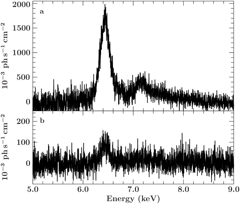
Figure 4: The iron line region of Vela X-1 can be nicely studied in this stacked residuals of all 88 XMM-Newton-spectra (a). The model includes the continuum shape only and, thus, does not take any fluorescent line emission into account. The residuals of the single spectrum with the highest signal show the K$\alpha$ emission line only (b). Note that the residual flux in this line is $\sim$15 times lower compared to the stacked residuals.

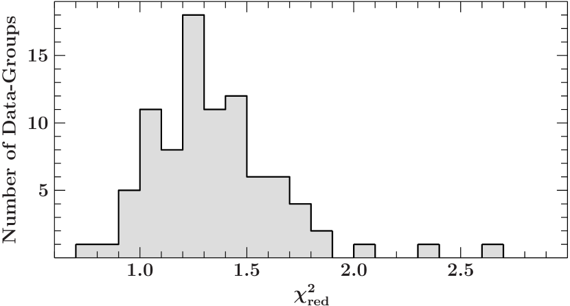
Figure 5: Example for a histogram of the goodness of the fits. Here, the distribution of the $\chi^{2}_{\mathrm{red}}$ of all individual data-groups of the 88 XMM-Newton-spectra of Vela X-1 are shown.

Another excellent example for a simultaneous fit was performed by martineznunez2014a [10]. These authors have analyzed 88 spectra recorded by XMM-Newton during a giant flare of Vela X-1. Although the continuum parameters were changing dramatically within the ${\sim}100$ ks observation a single model consisting of three absorbed power-laws is able to describe the data with a $\chi^{2}_{\mathrm{red}}=1.43$ with 9765 degrees of freedom [10]. Due to a global photon index for all power-laws and data-groups the absorption column densities and iron line fluxes could be constrained well.

Because every data-group is a single spectrum taken by the XMM-EPIC-PN camera and a common energy grid was used, the $\chi^{2}_{\mathrm{red,comb.}}$ equals the $\chi^{2}_{\mathrm{red}}$ here. Thus, it is preferred to calculate the stacked residuals of all data-groups according to Eq. 7. To demonstrate the advantage of this tool we have used the continuum model only, i.e. without any fluorescence line taken into account, and evaluated this model without any channel grouping to achieve the highest possible energy resolution. The resulting stacked residuals in the iron line region (5–9 keV) are shown in Fig. 4. The iron K$\alpha$ line at ${\sim}6.4$ keV and the K$\beta$ line at ${\sim}7.1$ keV are nicely resolved. The tail following the K$\beta$ line is probably caused by a slight mismatch of the continuum model with the data and requires a more detailed analysis. Note that the flux of this mismatch is a few $10^{-3}$ photons s^-1 cm^-2, which is detectable only in these stacked residuals featuring 100 ks exposure time and after the strong continuum variability on ks-timescales has been subtracted.

As a further demonstrative example, the histogram of the goodness of the fits of the 88 data-groups calculated after Eq. 4 is shown in Fig. 5. The median $\chi^{2}_{\mathrm{red}}$ is around 1.3, indicating that the model still could be improved slightly. Investigating the three outliers with $\chi^{2}_{\mathrm{red}}>2$ indeed proves that the residuals around in the iron line region are left, which are responsible for the high $\chi^{2}_{\mathrm{red}}$ and very similar to those shown in Fig. 4. There are no, however, extended residuals visible. Thus, the continuum parameters presented in martineznunez2014a [10] are still valid.

3.3 XTE J1859+083

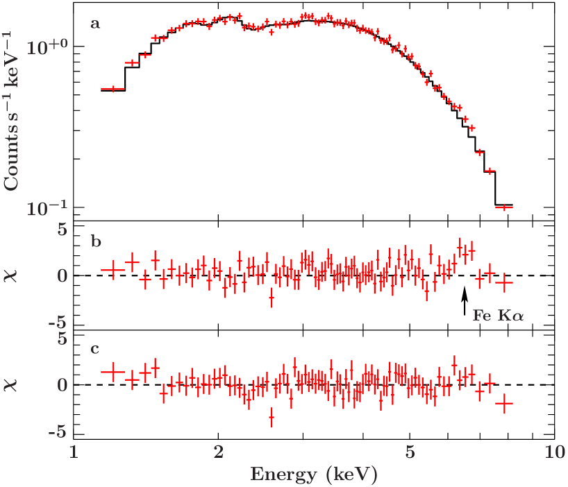
Figure 6: Seven stacked spectra of Swift-observations of XTE J1859+083 (a) and the residuals to the model (b). A weak iron K$\alpha$ emission line at 6.4 keV is visible, which is not detected in the residuals of any individual spectrum (c).

The last example shown in this work is the outburst of the transient pulsar XTE 1859+083 in 2015 April. This source was in quiescence since its bright outburst in 1996/1997 [11]. During the recent outburst several short observations by Swift were performed. A first analysis of these data in combination with INTEGRAL spectra reports an absorbed power-law shape of the source’s X-ray continuum [12]. We have extracted and analyzed seven Swift-XRT spectra and can confirm these findings. However, after examining the stacked residuals of all spectra an iron K$\alpha$ emission line at 6.4 keV shows up that has not been detected before (see Fig. 6). We define the equivalent width of this line as a global parameter and find a value of $60\pm 40$ eV (uncertainty is at the 90% confidence level, $\chi^{2}_{\mathrm{red,comb.}}=0.98$ with 585 degrees of freedom).

4 Summary

We have continued developing functions to handle simultaneous fits in ISIS, which we have introduced in paper I. In particular, we have concentrated on tools for checking the goodness of the fits to discover failed fits of individual data-groups or global discrepancies of the model. We propose to

• investigate the distribution of the goodness of fits to all individual data-groups

• calculate a combined goodness, here the $\bf\chi^{2}_{\mathrm{\bf red,comb.}}$, which takes the individual nature of each data-group into account

• look at the stacked residuals of all data-groups to reveal weak features

during a simultaneous fit in order to find the global best-fit. We have demonstrated the tremendous benefit of analyzing the stacked residuals by observations of three accreting neutron stars, in which we could identify weak features that had not been detected before.

- [1] M. Kühnel, S. Müller, I. Kreykenbohm, et al. Simultaneous Fits in ISIS on the Example of GRO J100857. Acta Pol 55:1–4, 2015.
- [2] J. C. Houck, L. A. Denicola. ISIS: An Interactive Spectral Interpretation System for High Resolution X-Xay Spectroscopy. In N. Manset, C. Veillet, D. Crabtree (eds.), Astronomical Data Analysis Software and Systems IX, vol. 216 of Astron. Soc. of the Pacific Conf. Series, p. 591. 2000.
- [3] K. A. Arnaud. XSPEC: The First Ten Years. In G. H. Jacoby, J. Barnes (eds.), Astronomical Data Analysis Software and Systems V, vol. 101 of Astron. Soc. of the Pacific Conf. Series, p. 17. 1996.
- [4] B. Anderson, J. Chiang, J. Cohen-Tanugi, et al. Using Likelihood for Combined Data Set Analysis. In Y. Fukazawa, Y. Tanaka, R. Itoh (eds.), Proceedings of the 5th Fermi Symposium, arXiv 1502.03081, 2015
- [5] C. Ricci, R. Walter, T. J.-L. Courvoisier, S. Paltani, Reflection in Seyfert galaxies and the unified model of AGN. A&A 532:A102, 2011.
- [6] E. Bulbul, M. Markevitch, A. Foster, et al. Detection of an Unidentified Emission Line in the Stacked X-Ray Spectrum of Galaxy Clusters. ApJ 789:13, 2014.
- [7] M. Kühnel, S. Müller, I. Kreykenbohm, et al. GRO J100857: an (almost) predictable transient X-ray binary. A&A 555:A95, 2013.
- [8] K. Jahoda, C. B. Markwardt, Y. Radeva, et al. Calibration of the Rossi X-Ray Timing Explorer Proportional Counter Array. ApJS 163:401–423, 2006.
- [9] J. A. García, J. E. McClintock, J. F. Steiner, et al. An Empirical Method for Improving the Quality of RXTE PCA Spectra. ApJ 794:73, 2014.
- [10] S. Martínez-Núñez, J. M. Torrejón, M. Kühnel, et al. The accretion environment in Vela X-1 during a flaring period using XMM-Newton. A&A 563:A70, 2014.
- [11] R. H. D. Corbet, J. J. M. in’t Zand, A. M. Levine, F. E. Marshall. Rossi X-Ray Timing Explorer and BeppoSAX Observations of the Transient X-Ray Pulsar XTE J1859+083. ApJ 695:30–35, 2009.
- [12] D. Malyshev, C. Ferrigno, D. Gotz. INTEGRAL measures the hard X-ray spectrum of the Be/X-ray binary XTE J1859+083. ATel 7425, 2015.