Exponential self-similar mixing by incompressible flows

Abstract.

We study the problem of the optimal mixing of a passive scalar under the action of an incompressible flow in two space dimensions. The scalar solves the continuity equation with a divergence-free velocity field, which satisfies a bound in the Sobolev space $W^{s,p}$, where $s\geq 0$ and $1\leq p\leq\infty$. The mixing properties are given in terms of a characteristic length scale, called the mixing scale. We consider two notions of mixing scale, one functional, expressed in terms of the homogeneous Sobolev norm $\dot{H}^{-1}$, the other geometric, related to rearrangements of sets. We study rates of decay in time of both scales under self-similar mixing. For the case $s=1$ and $1\leq p\leq\infty$ (including the case of Lipschitz continuous velocities, and the case of physical interest of enstrophy-constrained flows), we present examples of velocity fields and initial configurations for the scalar that saturate the exponential lower bound, established in previous works, on the time decay of both scales. We also present several consequences for the geometry of regular Lagrangian flows associated to Sobolev velocity fields.

1. Introduction

We study the problem of optimal mixing of scalar, passive tracers by incompressible flows. How well a quantity transported by a flow is mixed is an important problem in fluid mechanics and in many applied fields, for instance in atmospheric and oceanographic science, in biology, and in chemistry. In combustion, for example, fuel and air need to be well mixed for an efficient reaction to take place. In many situations, the interaction between the tracer and the flow can be neglected: mathematically, this results in the fact that the tracer solves a linear continuity equation with a given velocity field (see (1.2)). This problem is also a surprisingly rich source of questions in analysis, in particular relating partial differential equations and dynamical systems with geometric measure theory.

There is a well-established fluid mechanics literature concerning mixing and turbulence, especially with respect to statistical properties (see e.g. [12, 25] and references therein). It is known, in fact, that turbulent advection enhances mixing, which in turn can enhance diffusion and suppress concentration (see [18] for steady “relaxation enhancing” flows and [32] for an application to chemotaxis, for instance). Enhanced dissipation occurs also in Euler flows as an effect of inviscid Landau damping (see [9] and references therein). Mixing has also long been studied in the context of chaotic dynamics [7, 40, 36]. Indeed the decay to zero of the mixing scale defined in terms of negative Sobolev norms corresponds to ergodic mixing by the flow (as shown in [38]), and several well-known examples of discrete dynamical systems exhibit an exponential decay of correlations, which essentially means exponential mixing (however, these examples cannot be easily adapted to our context).

Recently there has been a renewed interest in quantifying the degree of mixing under an incompressible flow, and in producing examples that achieve optimal mixing. On the analytic side, progress has been possible in part due to the development of new tools to study transport and continuity equations under non-Lipschitz velocities [23, 5, 6], in particular quantitative estimates on regular Lagrangian flows [19]. On the applied and computational side, optimal mixing has been approached from the point of view of homogenization and control with more realistic models [35, 24]. Experiments have also been performed (see for example [26, 31, 30]).

1.1. The continuity equation.

We consider mixing in two space dimensions, as 2D is the first dimension with non-trivial, divergence-free fields and also for comparison with computational and experimental studies. Generally, dimension will not play a crucial role in what follows, except in setting scaling laws. However, it is technically more difficult to construct optimal mixers in two space dimensions, informally speaking for topological reasons. In fact, all our results can be extended to higher dimensions in a straightforward manner by making all quantities constant with respect to the additional independent variables. The divergence-free condition is a strong constraint that can be somewhat relaxed, but it is physically motivated in applications of mixing, and it is essential for the definition of the mixing scales we adopt. In fact, since we aim at producing examples of optimal mixing, the divergence-free condition is a more restrictive requirement that must be satisfied in our constructions.

We work on the two-dimensional torus $\mathbb{T}^{2}:=\mathbb{R}^{2}/\mathbb{Z}^{2}$ or on the plane $\mathbb{R}^{2}$. When considering the plane $\mathbb{R}^{2}$, both velocity fields and solutions eventually resulting from our constructions will be supported in a fixed compact set.

Given a divergence-free, time-dependent velocity field $u=u(t,x)$, we consider a scalar $\rho=\rho(t,x)\in L^{\infty}$ that is passively advected by $u$, i.e., a solution of the transport equation:

$$\partial_{t}\rho+u\cdot\nabla\rho=0.$$ (1.1)

Under the divergence-free assumption on the velocity $u$, the scalar $\rho$ is also a solution of the continuity equation:

$$\partial_{t}\rho+\mathop{\mathrm{div}}(u\rho)=0\,.$$ (1.2)

We prescribe an initial datum $\rho(0,\cdot)=\bar{\rho}$ at time $t=0$.

In the following we will always assume that the initial datum $\bar{\rho}$ has integral equal to $0$. Since the continuity equation (1.2) preserves the integral of the solution over the spatial domain along the time evolution, it follows that $\rho(t,\cdot)$ has zero integral for any time $t$. This fact is relevant when using negative Sobolev norms to measure mixing (see Definition 2.10, §2.1, and Remarks 2.2(i), 2.2(ii)).

1.2. Functional and geometric mixing scales.

In order to discuss the mixing properties of solutions to the continuity equation (1.2) we need to define a notion of mixing scale that can quantify the “level of mixedness” of the solution $\rho(t,\cdot)$ at time $t$. At least at a formal level, the continuity equation preserves all $L^{p}$ norms of the solution, which as a result are not a suitable measurement of mixing in our setting. Though, it is still possible for $\rho(t,\cdot)$ to converge to zero weakly. This is the mixing process we want to quantify and analyze in this paper.

We will employ and compare two notions of mixing scales that are considered in the literature. The first one is based on a negative Sobolev norm of the solution $\rho(t,\cdot)$, more precisely the norm in the homogeneous Sobolev space $\dot{H}^{-1}$ following [34] (see Definition 2.10 below, and see §2.1 for the definition of homogeneous Sobolev norms), and will be referred to as the functional mixing scale. In fact, it can be proven that the vanishing of the homogeneous negative Sobolev $\dot{H}^{-1}$ norm of $\rho(t,\cdot)$ is equivalent to the convergence of $\rho(t,\cdot)$ to $0$ weakly in $L^{2}$ (see for instance [34]). The use of negative norms to measure mixing was proposed in [39], where the equivalence between the decay of the $\dot{H}^{-1/2}$ norm and mixing in the ergodic sense was established. The second mixing scale arises from a conjecture of Bressan [15] on the cost of rearrangements of sets and brings in a connection with geometric measure theory. This second notion of scale is expresses in terms of how small the mean of the solution $\rho(t,\cdot)$ is on suitably small balls (see Definition 2.11 below), and it will be referred to as the geometric mixing scale. The two scales are related though generally not equivalent.

In the rest of this introduction, we informally denote any of the two mixing scales of the solution $\rho$ at time $t$ by $\mathrm{mix}\big{(}\rho(t,\cdot)\big{)}$.

Ideally, a flow that “mixes optimally” will achieve the largest decay rate in time for $\mathrm{mix}\big{(}\rho(t,\cdot)\big{)}$. How fast $\mathrm{mix}\big{(}\rho(t,\cdot)\big{)}$ can decay in time depends on properties of the flow. These, in turn, are in practice given in terms of constraints on certain quantities of physical interest, typically energy, enstrophy, and palenstrophy. These correspond respectively to uniform-in-time bounds on the $L^{2}$, $H^{1}$, and $H^{2}$ norms of the velocity field $u$.

1.3. Main results.

As described in detail in §1.5 below, it has been recently proven [19, 28, 42] that the (functional or geometric) mixing scale can decay at most exponentially in time:

$$\mathrm{mix}\big{(}\rho(t,\cdot)\big{)}\geq C\exp(-ct)\,,$$ (1.3)

if the velocity field satisfies a constraint on the Sobolev norm $W^{1,p}$ for some $1<p\leq\infty$, uniformly in time. Above, $C>0$ and $c>0$ are constant depending on the initial datum $\bar{\rho}$ and on the given bounds on the velocity field.

The primary goal of this work is to show the optimality of the bound (1.3) for all $1<p\leq\infty$, which was previously unknown (see however [45] and the brief description in §1.5 below). Our strongest result concerning the decay of the mixing scale can be stated as follows:

There exist a smooth, bounded, divergence-free velocity field $u$ which is Lipschitz uniformly in time, and a smooth, bounded, nontrivial solution $\rho$ of the continuity equation (1.2) such that the (functional or geometric) mixing scale of the solution decays exponentially in time:

$$\mathrm{mix}\big{(}\rho(t,\cdot)\big{)}\leq C\exp(-ct).$$ (1.4)

1.4. Remark.

1. It is very important to keep in mind the difference between the regularity allowed on the velocity field itself and the regularity spaces where the velocity satisfies bounds uniformly in time. In the above statement, describing our strongest result, the velocity field is smooth in space and time. However, the velocity is uniformly bounded in time only in the Sobolev spaces $W^{s,p}$ with $0\leq s\leq 1$ and $1\leq p\leq\infty$. If $s>1$, the velocity is bounded in $W^{s,p}$ on any finite time interval $[0,T]$, $0<T<\infty$, but the norm blows up when $t\to\infty$.

2. The construction that leads to the main result stated above also yields examples of regular velocity fields and smooth solutions exhibiting different rates of decay for the mixing scale which depend on the uniform-in-time bounds for the Sobolev norms of the velocity field. More precisely, if we ask that the velocity field is uniformly bounded in time in the Sobolev space $W^{s,p}$ for some $s\geq 0$ and some $1\leq p\leq\infty$, then we can construct examples such that:

   • If $s<1$, there exists a time $t^{*}$ such that $\mathrm{mix}\big{(}\rho(t^{*},\cdot)\big{)}=0$, that is, perfect mixing is achieved in finite time;

   • If $s=1$, the mixing scale decays exponentially, that is, (1.4) holds;

   • If $s>1$, the mixing scale decays polynomially, that is, there exists an exponent $\alpha=\alpha(s)>0$ such that $\mathrm{mix}\big{(}\rho(t,\cdot)\big{)}\leq Ct^{-\alpha}$.

Further remarks are detailed in §1.6 and §1.8 below. The results presented in this article were announced in [3].

Before making further observations on our results and techniques we make a digression about the past literature on this topic.

1.5. Past literature.

Mixing phenomena are studied in the literature under energetic constraints on the velocity field, that is, assuming that the velocity field is bounded with respect to some spatial norm, uniformly in time. This research area is related in a very natural way to the study of transport and continuity equations under non-Lipschitz velocities (see [6] for a recent survey). We survey key results in the literature on both areas (most of the results hold in any space dimension):

1. The velocity field $u$ is bounded in $W^{s,p}$ uniformly in time for some $s<1$ and $1\leq p\leq\infty$ (the case $s=0$, $p=2$, relevant for applications, is often referred to as energy-constrained flow). In this case, in general there is no uniqueness for the solution to the Cauchy problem for the continuity equation (1.2) (see [2, 1]). Hence, one can find a velocity field and a bounded solution which is non-zero at the initial time, but is identically zero at some later time. Therefore it is possible to have perfect mixing in finite time, as already observed in [34] and established in [37] for $s=0$, building on examples from [21, 15].

2. The velocity field $u$ is bounded in $W^{1,p}$ uniformly in time for some $1\leq p\leq\infty$ (the case $p=2$, relevant for applications, is often referred to as enstrophy-constrained flow). The theory in [23] guarantees uniqueness for the Cauchy problem (1.2), which in particular excludes perfect mixing in finite time. A quantification of the maximal decay rate for the mixing scale has been achieved thanks to the quantitative estimates for regular Lagrangian flows in [19]. In detail, for $p>1$, the theory in [19] provides an exponential lower bound on the geometric mixing scale (see (1.3)). The extension to the borderline case $p=1$ is still open (see, however, [13]). The same exponential lower bound (1.3) has been proved for the functional mixing scale in [28, 42]. See also  [33, 16] for further results on these bounds. More recently, in [14] the authors were able to prove regularity estimates for the solution of the continuity equation by studying the propagation of a weighted norm of the solution, without the assumption of bounded divergence on the velocity.

3. The theory in [5] provides uniqueness for the Cauchy problem (1.2) for velocity fields bounded in $BV$ uniformly in time (see also [11], in which the divergence-free assumption is replaced by the more general condition of near incompressibility). Again, uniqueness excludes perfect mixing in finite time. The validity of the bound (1.3) is still unknown in this context. However, in [15] it is observed that such an exponential decay of the geometric mixing scale can indeed be attained for velocity fields bounded in $BV$ uniformly in time. The same example works also for the functional mixing scale.

4. The velocity field $u$ is bounded in $W^{s,p}$ uniformly in time for some $s>1$ and $1\leq p\leq\infty$ (the case $s=2$ and $p=2$, relevant for applications, goes under the name of palenstrophy-constrained flow). In this case, Estimate (1.3) gives immediately an exponential lower bound for both mixing scales. However, it is still open whether such a bound is sharp or not. Numerical simulations, such as those in [37, 28], and heuristic arguments support the optimality of the exponential decay. (See also the discussion in §1.8.)

The constants $C$ and $c$ in (1.3) depend not only on the given bounds for the velocity field, but also on the initial datum $\bar{\rho}$ (not simply through its mixing scale). In fact, it is not clear that an estimate of the form

$$\mathrm{mix}\big{(}\rho(t,\cdot)\big{)}\geq C\,\mathrm{mix}(\bar{\rho})\exp(-ct),$$

with $C$ and $c$ constants depending only on the given bounds on the velocity field, can be achieved. It is then natural to ask whether it is possible to obtain bounds on the rate of decay with constants that only depend on the mixing scale of the initial datum, and not on its geometry. Unfortunately, direct PDE methods, such as energy estimate, do not seem to yield sharp bounds: for instance, they yield a Gaussian bound for palenstrophy-constrained flows, while the optimal bound is at least exponential (see [37]).

There are examples in the literature of enstrophy-constrained flows that saturate the exponential decay rate complementary to those presented in this work (§1.3). Yao and Zlatoš [45] utilize a cellular flow to obtain decay of the mixing scale for any bounded initial datum $\bar{\rho}$ (where the flow depends on $\bar{\rho}$), under a $W^{1,p}$ constraint on the velocity field for any $1\leq p\leq\infty$. The decay rate is optimal in the range $1<p<\bar{p}$ for some explicit $\bar{p}>2$. They also give an interesting result on “unmixing” a given configuration. (See also §1.8 for a comparison of our results with those from [45].)

Before these recent analytic results, numerical experiments were performed that supported an exponential rate of decay for $\mathrm{mix}\big{(}\rho(t,\cdot)\big{)}$ under an enstrophy constraint. For instance, a numerical scheme to compute an instantaneous optimizer was given in [34], and numerical tests performed for a sinusoidal initial configuration. A global optimizer was computed numerically in [38].

Our approach to finding optimal mixers is constructive and is essentially based on a self-similar scheme. We actually present two related, but distinct constructions: the first one, referred to as the self-similar construction, is simpler and self-similar in a strict sense. This first construction allows us to obtain only examples where the velocity field is neither smooth nor uniformly bounded in $W^{1,\infty}$. The second construction, which we refer to as the quasi-self-similar construction, is more involved and allows us to construct examples where the velocity is smooth, and uniformly bounded in $W^{1,\infty}$.

We do not claim that a self-similar evolution is more physical (however, see [41]) or preferred over other types. The only reason for choosing (quasi) self-similar constructions is that it makes the mixing scale of (some) solutions easier to estimate.

1.6. Self-similar construction.

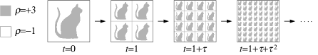
Figure 1. Example of self-similar evolution for a function $\rho$ taking only two values.

Briefly, the construction starts from a “basic move”, which is just a pair of a velocity field and a weak solution of the associated continuity equation (quite often the characteristic function of a set) and consists in combining infinitely many copies of this basic move, suitably rescaled in time and space, so to obtain a velocity field and a solution with the desired features (the reader can glimpse at the self-similar construction in Figure 1). More precisely, the construction is divided in three steps:

1. Scaling analysis (Section 3): we assume the existence of a basic move (velocity field and solution) defined for the times $0\leq t\leq 1$ with a certain regularity, and describe the self-similar construction that gives a new velocity field and solution defined for all times $t\geq 0$. We then analyze the decay of the mixing scale of this new solution and the behavior of the Sobolev norms of the new velocity field.

2. Geometric tools (Section 4): we establish a series of geometric lemmas that guarantee the existence of smooth, divergence-free velocity fields with the property that the associated flows deform smooth sets according to a prescribed evolution in time.

3. Construction of the basic move (Section 5): we use such geometric tools to construct the basic move we need in Step I. The solution is the characteristic function of a regular set that evolves smoothly for all times except finitely many singular times. The main technical point here is to deal with the possible singularities present.

We stress that the regularity of (and the bounds on) the velocity field and the regularity of the solution constructed in Step I above depend only on the regularity of (and the bounds on) the basic move. So far, using a strictly self-similar approach, we have only been able to construct a basic move with velocity of class $W^{1,p}$ with $p<\infty$.

1.7. Quasi-self-similar construction.

To construct examples of exponential decay of the mixing scale of the solution with a velocity field which is bounded in $W^{1,\infty}$ uniformly in time (as claimed in §1.3), we use a construction which is not exactly self-similar. The main difference is that we combine rescaled copies not of just one basic move, but of a (finite) family of basic moves. Using this more flexible setting we can actually construct velocity fields and solutions that are smooth in both space and time.

Of the three steps mentioned above, Step I is unchanged except that we assume the existence of a family of (smooth) basic moves (see Section 6). Step II consists of some improvements of the geometric lemmas established in Section 4 (see Section 7). Finally Step III consists as before of the construction of the basic moves (Section 8). In this second construction, the regularity of the velocity field does not depend just on the regularity of the basic moves, but also on the details of how the rescaled moves are glued together and on the overall combinatorial aspects of the construction (see for instance Figure 9).

Given that the basic moves are smooth and hence in $W^{s,p}$ for any $s\geq 0$ and $1\leq p\leq\infty$, the analysis in Step I can be performed for any such $s$ and $p$. However, the bounds on the Sobolev norms of the velocity field and the decay of the mixing scale depend on the specific rescaling of the basic moves.

It turns out that an exponential decay of the mixing scale of the solution can only be obtained with a uniform bound on the Sobolev norms of the velocity with $s=1$ (regardless of $p$). Vice versa, examples with a uniform bound on the Sobolev norms of the velocity with $s>1$ can only be obtained with a polynomial decay of the mixing scale of the solution (see the discussion in Remark 1.4(ii)). In particular, in our examples of palenstrophy-constrained velocity the mixing scale decays only at a polynomial rate rather than the expected exponential rate (recall §1.5(d)). Whether exponential rate can be obtained is open in this case.

1.8. Further remarks and open problems.

Our main result is a proof that the bound (1.3) is optimal. In order to do so, we construct one velocity field which is bounded in $W^{1,p}$ uniformly in time for any $1\leq p\leq\infty$, and one solution, the mixing scale of which decays exponentially. In fact, following the strategy described above, it is possible to construct a large class of initial data for which the mixing scale decays exponentially. However, it is unclear whether this is the case for every initial datum. The following questions about the existence of “universal mixers” are therefore natural.

1. Given any bounded initial datum $\bar{\rho}$, is there a velocity field, bounded in $W^{1,p}$ uniformly in time and possibly dependent on $\bar{\rho}$, such that $\mathrm{mix}\big{(}\rho(t,\cdot)\big{)}$ decays to zero?

2. If the answer to Question (a) is positive, does this velocity field drive the mixing scale of $\rho$ to zero exponentially in time? Since, in principle, answers to Question (a) may not be unique given $\bar{\rho}$, we are seeking at least one such velocity field.

3. Does there exist one velocity field, bounded in $W^{1,p}$ uniformly in time, such that $\mathrm{mix}\big{(}\rho(t,\cdot)\big{)}$ decays to zero for every bounded initial datum $\bar{\rho}$?

4. If the answer to Question (c) is positive, does this velocity field drive the mixing scale of $\rho$ to zero exponentially in time? The same comment about uniqueness in Question (b) applies here.

We observed in Remark 1.4(ii) that our construction provides an example of palenstrophy-constrained flow such that $\mathrm{mix}\big{(}\rho(t,\cdot)\big{)}$ decays polynomially in time. In fact, the self-similarity ansatz implies polynomial decay of $\mathrm{mix}\big{(}\rho(t,\cdot)\big{)}$ under the assumption that the velocity field is bounded in $W^{s,p}$ uniformly in time for some $s>1$. However, the numerical results mentioned in §1.5(d) support an exponential decay also for $s>1$, but the optimal bound is still unknown in this case. If the optimal decay were indeed exponential, we would then deduce that for $s>1$ self-similarity is too restrictive and only allows for sub-optimal decay rates. Such a result would be in stark contrast with the case $s=1$, for which the optimal decay rate can be achieved with a self-similar evolution. We therefore formulate the following important question:

1. Do a bounded initial datum $\bar{\rho}$ and a velocity field, which is bounded in $W^{s,p}$ uniformly in time for some $s>1$, exist such that $\mathrm{mix}\big{(}\rho(t,\cdot)\big{)}$ decays exponentially in time?

Such an example could not then be self-similar. In addition, the analysis in [20] implies that it cannot be realized with a “localized” flow: roughly speaking, once the solution has been mixed to a certain scale, it can be more convenient to let the flow act again at larger scales before reaching a lower mixing scale.

As mentioned in §1.5, examples of enstrophy-constrained flows that saturate the exponential decay rate (1.3) have been constructed in [45]. There, the authors utilize a cellular flow consisting of pseudo-rotations on a family of nested tilings of the square, and are able to obtain exponential mixing of every bounded initial datum $\bar{\rho}$ by means of a velocity field, which depends on $\bar{\rho}$ in general, bounded in $W^{1,p}$ uniformly in time in the range $1\leq p<\bar{p}$ for some $\bar{p}>2$. Therefore, this construction provides a partial answer to Question (b) above. Their nice geometric argument is based on a “stopping time” for the pseudo-rotation, which is determined by a clever application of the intermediate value theorem for continuous functions. Their construction also applies in the range $\bar{p}\leq p\leq\infty$, giving a mixing rate which is slightly slower than exponential, thus answering Question (a) above.

In comparison with [45], while we obtain exponential mixing of the solution in the full range $1\leq p\leq\infty$, including the Lipschitz case, our construction applies only to certain specific initial data. Our strategy has a geometric flavor and generates velocity fields and solutions that are smooth. This last fact is relevant for the full scaling analysis (recall Remark 1.4(ii)) and for the application to the study of the loss of regularity for continuity equations, which is addressed in the companion paper [4] (see §1.10 for a brief discussion). In addition, our examples provide an important insight into the geometrical properties of regular Lagrangian flows.

1.9. Geometry of regular Lagrangian flows.

When the velocity field is Lipschitz (as in the quasi-self-similar examples) then the associated flow is well-defined in the classical sense, and there is not much to add. However, when the velocity field has singularities and belongs only to some Sobolev class (as in the self-similar examples) then the flow is no longer well defined in the classical sense, and one should instead consider the notion of regular Lagrangian flow. We stress that the regular Lagrangian flow associated to our self-similar examples has the following additional properties:

• the associated regular Lagrangian flow does not preserve the property of a set of being connected;

• there exists a segment that is collapsed to a point and, subsequently, inflated back to a full segment in finite time under this regular Lagrangian flow;

• as a consequence, the trajectories of the velocity field (that is, the solutions of the associated ODE) which start at a point in this segment are non unique.

1.10. Loss of regularity for continuity equations.

Mixing leads to growth of positive Sobolev norms of the solution $\rho$, saturating the exponential growth which follows from the classical Grönwall inequality. Analytically, this result is a consequence of the preservation of the $L^{2}$-norm of the solution and of the exponential decay of the negative Sobolev norms in (1.4) by an interpolation argument.

In the companion paper [4], we present an example of a velocity field in $W^{1,p}$ for any $1\leq p<\infty$ that is regular except at a point and of a smooth $\bar{\rho}$, such that the corresponding solution of (1.2) leaves any Sobolev space $H^{s}$ with $s>0$ instantaneously for $t>0$. Extensions of this construction to non-Lipschitz fields with Sobolev regularity of order higher than $1$ are also possible.

Lack of propagation of $C^{0}$ and of $BV$ regularity for solutions of the continuity equation was already observed in [17]. More recently, in [29] it was observed that Sobolev regularity of order one does not transfer from a velocity field to its associated flow, using a different construction that exploits a randomization procedure on certain basic elements of the flow.

0. Acknowledgments.

The first and third authors acknowledge the hospitality of the Department of Mathematics and Computer Science at the University of Basel, where this work was started. Their stay was partially supported by the Swiss National Science Foundation grants 140232 and 156112. The visits of the second author to Pisa were supported by the University of Pisa PRA project “Metodi variazionali per problemi geometrici [Variational Methods for Geometric Problems]”. The second author was partially supported by the ERC Starting Grant 676675 FLIRT and third author by the US National Science Foundation grants DMS 1312727 and 1615457.

2. Preliminaries

Throughout the paper, we will make extensive use of homogeneous Sobolev spaces with real order of differentiability and of their properties. We present here their definition and main properties of interest for our work, namely those regarding scaling, interpolation, and embeddings. For a systematic exposition we refer the reader to [10, 8, 22, 27, 44]. In addition, in the last part of this section, we define the two notions of mixing scale that we will use in our work.

We limit our presentation to the two-dimensional case, however all definitions and results can be extended with obvious changes to the case of higher space dimensions. We work both on the plane $\mathbb{R}^{2}$ and on the two-dimensional flat torus $\mathbb{T}^{2}:=\mathbb{R}^{2}/\mathbb{Z}^{2}$. The Fourier transform of a tempered distribution $f$ on $\mathbb{R}^{2}$ is denoted by $\hat{f}(\xi)$; the Fourier coefficients of a distribution $f$ on $\mathbb{T}^{2}$ are denoted by $\hat{f}(k)$.

2.1. Homogeneous Sobolev spaces $\boldsymbol{\dot{H}^{s}}$.

For $s\in\mathbb{R}$, we say that a distribution $f$ on $\mathbb{T}^{2}$ belongs to the homogeneous Sobolev space $\dot{H}^{s}(\mathbb{T}^{2})$ if

$$\|f\|^{2}_{\dot{H}^{s}(\mathbb{T}^{2})}:=\sum_{k\in\mathbb{Z}^{2}}|k|^{2s}|\hat{f}(k)|^{2}<\infty\,.$$ (2.1)

We say that a tempered distribution $f$ on $\mathbb{R}^{2}$ belongs to the homogeneous Sobolev space $\dot{H}^{s}(\mathbb{R}^{2})$ if $\hat{f}\in L^{1}_{\rm loc}(\mathbb{R}^{2})$ and

$$\|f\|^{2}_{\dot{H}^{s}(\mathbb{R}^{2})}:=\int_{\mathbb{R}^{2}}|\xi|^{2s}|\hat{f}(\xi)|^{2}\,d\xi<\infty\,.$$ (2.2)

This definition is suitable for our purposes, though it is different from the standard definition, which requires the use of equivalence classes modulo polynomials (see e.g. [27, 44]).

We remark that homogeneous Sobolev spaces do not form a scale, due to the singularity of the multiplier at the origin in frequency space. In particular, it is generally not true that any square integrable function is automatically in $\dot{H}^{s}$, for $s<0$.

2.2. Remark.

1. From (2.1) we immediately recognize that, in order for a function $f\in L^{2}(\mathbb{T}^{2})$ to belong to some $\dot{H}^{s}(\mathbb{T}^{2})$ with $s<0$, it is necessary that $\hat{f}(0)=0$. This corresponds to the zero-integral condition $\int_{\mathbb{T}^{2}}f=0$. Conversely, let $f\in L^{2}(\mathbb{T}^{2})$ be a function with zero integral: since the sequence of its Fourier coefficients $\{\hat{f}(k)\}_{k\in\mathbb{Z}^{2}}$ belongs to $\ell^{2}$, we deduce that such a function necessarily belongs to $\dot{H}^{s}(\mathbb{T}^{2})$ for every $s\leq 0$.

2. Given a function $f\in L^{1}(\mathbb{R}^{2})$, its Fourier transform $\hat{f}$ is continuous. If ${s\leq-1}$ the singularity at $\xi=0$ in (2.2) is not integrable, unless $\hat{f}(0)=0$. This means that the condition $\int_{\mathbb{R}^{2}}f=0$ is a necessary condition for $f$ to belong to $\dot{H}^{s}(\mathbb{R}^{2})$ with $s\leq-1$.

3. Let $f\in L^{2}(\mathbb{R}^{2})$ have compact support and zero integral. Paley-Wiener theorem implies that the Fourier transform $\hat{f}$ is analytic. In particular, there is a constant $C>0$ for which $|\hat{f}(\xi)|=|\hat{f}(\xi)-\hat{f}(0)|\leq C|\xi|$ for any ${|\xi|\leq 1}$, therefore the singularity at $\xi=0$ in (2.2) is integrable for every ${s>-2}$. Since ${\hat{f}\in L^{2}(\mathbb{R}^{2})}$, we conclude that $f\in\dot{H}^{s}(\mathbb{R}^{2})$ for any $-2<s\leq 0$.

2.3. Homogeneous Sobolev spaces $\boldsymbol{\dot{W}^{s,p}}$.

In the particular case $s\geq 0$ we extend the definition in §2.1 to an arbitrary summability exponent $1<p<\infty$. We say that a distribution $f$ on $\mathbb{T}^{2}$ belongs to the homogeneous Sobolev space $\dot{W}^{s,p}(\mathbb{T}^{2})$ if

$$\sum_{k\in\mathbb{Z}^{2}}|k|^{s}\hat{f}(k)e^{ikx}\in L^{p}(\mathbb{T}^{2})\,,$$ (2.3)

and we let $\smash{\|f\|_{\dot{W}^{s,p}(\mathbb{T}^{2})}}$ be the $L^{p}(\mathbb{T}^{2})$ norm of the function in (2.3). We observe that this definition gives a seminorm and not a norm, in general.

We say that a tempered distribution $f$ on $\mathbb{R}^{2}$ belongs to the homogeneous Sobolev space $\dot{W}^{s,p}(\mathbb{R}^{2})$ if $\hat{f}\in L^{1}_{\rm loc}(\mathbb{R}^{2})$ and

$$\mathscr{F}^{-1}\big{(}|\xi|^{s}\hat{f}(\xi)\big{)}\in L^{p}(\mathbb{R}^{2})$$ (2.4)

where $\mathscr{F}^{-1}$ is the inverse of the Fourier transform, and we let $\smash{\|f\|_{\dot{W}^{s,p}(\mathbb{R}^{2})}}$ be the $L^{p}(\mathbb{R}^{2})$ norm of the function in (2.4).

The condition that $\smash{\hat{f}\in L^{1}_{\rm loc}(\mathbb{R}^{2})}$ guarantees that this quantity is a norm. We have the obvious identification $\dot{W}^{s,2}\equiv\dot{H}^{s}$.

In our work, homogeneous spaces will be used only to measure the “size” of given functions and velocity fields, which will be typically regular. We can avoid to give a rigorous and complete definition of these spaces, which again is based on equivalence of distributions modulo polynomials, as we can just rely on the seminorms defined above. (We refer to e.g. [27, 44] for a more detailed discussion of these spaces.)

2.4. Remark.

1. The non-homogeneous Sobolev spaces $H^{s}$ and $W^{s,p}$ are defined by replacing in (2.1), (2.2), (2.3), and (2.4) the $|k|$ and $|\xi|$ by the symbols $\langle k\rangle:=\sqrt{1+|k|^{2}}$ and $\langle\xi\rangle:=\sqrt{1+|\xi|^{2}}$, respectively. If $s\in\mathbb{N}$ then $H^{s}$ and $W^{s,p}$ coincide with the usual Sobolev spaces defined using weak derivatives.

2. In the case of the plane $\mathbb{R}^{2}$, if we consider functions that are supported in a fixed compact set then the homogeneous and the non-homogeneous norms are equivalent, and therefore the homogeneous and the non-homogeneous spaces coincide. In the case of the torus $\mathbb{T}^{2}$, the homogeneous and the non-homogeneous spaces always coincide. The non-homogeneous norm is equivalent to the sum of the homogeneous norm and the $L^{2}$ norm.

3. In contrast to the case of negative spaces (see Remarks 2.2(i), 2.2(ii)), it is not necessary for functions to have zero average to belong to $\dot{W}^{s,p}$ with $s\geq 0$.

4. Let $K$ be a compact set contained in the open square $\mathscr{Q}=(-1/2,1/2)^{2}$. Let $\sigma$ be the canonical projection of the plane $\mathbb{R}^{2}$ onto the torus $\mathbb{T}^{2}=\mathbb{R}^{2}/\mathbb{Z}^{2}$. The restriction of $\sigma$ to $(-1/2,1/2)^{2}$ is a diffeomorphism. A Sobolev function $f$ on $\mathbb{R}^{2}$ with support contained in $K$ can be identified with a Sobolev function $\tilde{f}$ on $\mathbb{T}^{2}$ via the formula $\tilde{f}=f\circ\sigma^{-1}$. It can be shown that, if $s\geq 0$ and $1<p<\infty$, then

   $$C^{-1}\|f\|_{\dot{W}^{s,p}(\mathbb{R}^{2})}\leq\|\tilde{f}\|_{\dot{W}^{s,p}(\mathbb{T}^{2})}\leq C\|f\|_{\dot{W}^{s,p}(\mathbb{R}^{2})}\,,$$

   where the constant $C$ depends on $s$, $p$, and on the compact set $K$ (see [43]).

2.5. Lipschitz-Hölder spaces.

For notational convenience, in this paper we denote by $\dot{W}^{s,\infty}(\mathbb{T}^{2})$ and $\dot{W}^{s,\infty}(\mathbb{R}^{2})$ the homogeneous Lipschitz-Hölder spaces defined as follows (we do not write explicitly the domain).

If $s$ is a positive integer, we say that a function $f$ belongs to $\dot{W}^{s,\infty}$ if $f\in C^{s-1}$ and there is a constant $C>0$ such that

$$|f^{(s-1)}(x)-f^{(s-1)}(y)|\leq C|x-y|\quad\text{for every $x$ and $y$.}$$ (2.5)

We let $\|f\|_{\dot{W}^{k,\infty}}$ be the minimal constant $C$ for which (2.5) holds.

If $s\geq 0$ is not an integer, we let $\lfloor s\rfloor$ be the largest integer smaller than $s$, and we say that a function $f$ belongs to $\dot{W}^{s,\infty}$ if $f\in C^{\lfloor s\rfloor}$ and there is a constant $C>0$ such that

$$|f^{(\lfloor s\rfloor)}(x)-f^{(\lfloor s\rfloor)}(y)|\leq C|x-y|^{s-\lfloor s\rfloor}\quad\text{for every $x$ and $y$.}$$ (2.6)

We let $\|f\|_{\dot{W}^{s,\infty}}$ be the minimal constant $C$ for which (2.6) holds.

2.6. Remark.

In two space dimensions, the Sobolev space $\dot{W}^{s,p}$ embeds in the Lipschitz space $\dot{W}^{1,\infty}$ if $s>1$ and $p>\frac{2}{s-1}$.

2.7. Scaling properties.

We will be frequently interested in the behavior of homogeneous Sobolev norms under rescaling. Given $\lambda>0$ and a function $f$, we set

$$f_{\lambda}(x):=f\left(\frac{x}{\lambda}\right)\,.$$ (2.7)

If $f$ is defined on the torus and $1/\lambda$ is an integer, then the function $f_{\lambda}$ in (2.7) is well defined on the torus and it holds

$$\|f_{\lambda}\|_{\dot{W}^{s,p}(\mathbb{T}^{2})}=\lambda^{-s}\,\|f\|_{\dot{W}^{s,p}(\mathbb{T}^{2})}\,.$$ (2.8)

If $f$ is defined on the plane, then the function $f_{\lambda}$ in (2.7) is well defined for any $\lambda>0$ and it holds

$$\|f_{\lambda}\|_{\dot{W}^{s,p}(\mathbb{R}^{2})}=\lambda^{\frac{2}{p}-s}\,\|f\|_{\dot{W}^{s,p}(\mathbb{R}^{2})}\,.$$ (2.9)

When $p=2$, both formulas (2.8) and (2.9) hold also for $s<0$.

2.8. Remark.

The difference between the exponents in formulas (2.8) and (2.9) is due to the fact that, in the case of the torus, we are not changing the period, hence the measure of the torus, when rescaling. In particular, the rescaling of a single bump on the plane remains a single bump, while on the torus $1/\lambda^{2}$ rescaled copies of the bump are produced.

2.9. Interpolation.

We will frequently rely on the following standard interpolation inequality. If $s_{1}<s<s_{2}$ and $s=\vartheta s_{1}+(1-\vartheta)s_{2}$, $\vartheta\in(0,1)$, then

$$\|f\|_{\dot{H}^{s}}\leq\|f\|_{\dot{H}^{s_{1}}}^{\vartheta}\|f\|_{\dot{H}^{s_{2}}}^{1-\vartheta}$$ (2.10)

and

$$\|f\|_{\dot{W}^{s,p}}\leq\|f\|_{\dot{W}^{s_{1},p}}^{\vartheta}\|f\|_{\dot{W}^{s_{2},p}}^{1-\vartheta}\,,$$ (2.11)

where both inequalities hold both with domain $\mathbb{T}^{2}$ and $\mathbb{R}^{2}$. The same holds in the case $p=\infty$ in the context of Lipschitz-Hölder spaces (recall §2.5) and can be proven with a simple direct argument.

We next introduce the two notions of mixing scale that will be employed in this paper to quantify the level of mixedness of the solution $\rho$. Both definitions can be given on the torus and on the plane, and will be stated for functions of space variables only with zero integral. In our framework, the mixing scales of the solution will of course depend on time, due to the fact that the solution is dependent on time.

2.10. Functional mixing scale [34, 39].

Assume that $\rho$ has zero integral. The functional mixing scale of $\rho$ is $\|\rho\|_{\dot{H}^{-1}}$.

2.11. Geometric mixing scale [15].

Assume that $\rho$ has zero integral. Given $0<\kappa<1$, the geometric mixing scale of $\rho$ is the infimum of all $\varepsilon>0$ such that, for every $x\in{\mathbb{T}}^{2}$, there holds

$$\frac{1}{\|\rho\|_{\infty}}\left|\mkern 12.0mu\hbox{\vrule height=4.0pt,depth=-3.2pt,width=5.0pt}\mkern-16.5mu\int_{B_{\varepsilon}(x)}\rho\,dy\right|\leq\kappa\,.$$ (2.12)

The parameter $\kappa$ is fixed and plays a minor role in the definition. Informally, in order for $\rho$ to have geometric mixing scale $\varepsilon$, the average of the solution on every ball of radius $\varepsilon$ is essentially zero. Alternatively, the property of having (approximately) zero average needs to be localizable to balls of radius $\varepsilon$.

2.12. Remark.

The geometric mixing scale has been originally introduced in [15] for solutions with value $\pm 1$: given $0<\tilde{\kappa}<1/2$, (2.12) is replaced by the requirement that

$$\tilde{\kappa}\leq\frac{|\{\rho=1\}\cap B_{\varepsilon}(x)|}{|B_{\varepsilon}(x)|}\leq 1-\tilde{\kappa}\,.$$ (2.13)

Informally, in order for $\rho$ to have geometric mixing scale $\varepsilon$, every ball of radius $\varepsilon$ contains a “substantial portion” of both level sets $\{\rho=1\}$ and $\{\rho=-1\}$. The more general definition we adopt (see Definition 2.11) has been introduced in [45] and it applies to every bounded solution $\rho$, without any constraint on its values. It is easily seen that (2.12) and (2.13) correspond if $\kappa=1-2\tilde{\kappa}$.

As previously mentioned, the two notions of mixing scale are not equivalent, though they are strongly related (we refer to [37, 46] for a further discussion on this point; see also Lemma 3.5).

3. Scaling analysis in a self-similar construction

A conceivable procedure for mixing consists of a self-similar evolution. Such a procedure, together with the related scaling analysis, has been presented in [3]. We work on the torus $\mathbb{T}^{2}$. We let $s\geq 0$ and $1\leq p\leq\infty$ be fixed and we make the following assumption.

3.1. Assumption: self-similar base element.

There exist a velocity field $u_{0}$ and a (not identically zero) solution $\rho_{0}$ to (1.2), both defined for $0\leq t\leq 1$ and $x\in\mathbb{T}^{2}$, such that:

1. $u_{0}$ is bounded, bounded in $\dot{W}^{s,p}({\mathbb{T}}^{2})$ uniformly in time, and divergence-free;

2. $\rho_{0}$ is bounded and has mean zero for all times;

3. there exists a positive constant $\lambda$, with $1/\lambda$ an integer greater or equal than $2$, such that

   $$\rho_{0}(1,x)=\rho_{0}\left(0,\frac{x}{\lambda}\right)\,.$$

An explicit example of a $u_{0}$ and a $\rho_{0}$ satisfying these assumption will be given in Section 5 for $s=1$ and arbitrary $1\leq p<\infty$. In fact, the range of indices for this example is slightly larger (see (5.1)). However, it is not evident to us how to construct an example that satisfies Assumption 3.1 outside the range in (5.1), in particular for the case $s=1$ and $p=\infty$. This limitation leads us to introduce the second geometric construction in §6.

For later use, we introduce the following definition.

3.2. Definition.

Given $\lambda>0$, with $1/\lambda$ an integer, we denote by $\mathcal{T}_{\lambda}$ the tiling of $\mathbb{T}^{2}$ consisting of $1/\lambda^{2}$ open squares of side-length $\lambda$ in $\mathbb{T}^{2}$ of the form

$$\left\{(x,y)\in{\mathbb{T}}^{2}\,:\,\text{$(k-1)\lambda<x<k\lambda$ and $(h-1)\lambda<y<h\lambda$}\right\}\,,$$

with $k,h=1,2,\ldots,1/\lambda$.

Denoting by $\mathscr{Q}$ the unit open square $(-1/2,1/2)^{2}\subset\mathbb{R}^{2}$, the tiling $\mathcal{T}_{\lambda}$ of $\mathscr{Q}$ is defined in a similar way. Given any square $Q\in\mathcal{T}_{\lambda}$, we denote by $r_{Q}$ its center, so that $Q=\lambda\mathscr{Q}+r_{Q}$.

3.3. A self-similar construction.

We begin by fixing a positive number $\tau$ (to be determined later). Under Assumption 3.1, for each integer $n=1,2,\ldots$ and for $t\in[0,\tau^{n}]$ we set

$$u_{n}(t,x):=\frac{\lambda^{n}}{\tau^{n}}\;u_{0}\left(\frac{t}{\tau^{n}},\frac{x}{\lambda^{n}}\right)\,,\quad\rho_{n}(t,x):=\rho_{0}\left(\frac{t}{\tau^{n}},\frac{x}{\lambda^{n}}\right)\,.$$

Then $\rho_{n}$ is a solution of (1.2) corresponding to the velocity field $u_{n}$. Moreover, because of Assumption 3.1(iii),

$$\rho_{n}(\tau^{n},x)=\rho_{n+1}(0,x)\,.$$ (3.1)

We now define $u$ and $\rho$ by concatenating the velocity fields $u_{0},u_{1},\ldots$ and the corresponding solutions $\rho_{0},\rho_{1},\ldots$. In detail, we let

$$u(t,x):=u_{n}(t-T_{n},x)\,,\quad\rho(t,x):=\rho_{n}(t-T_{n},x)$$

for $T_{n}\leq t<T_{n+1}$, and $n=1,2,\ldots$, where

$$T_{n}:=\sum_{i=0}^{n-1}\tau^{i}\quad\text{for $n=1,2,\ldots,\infty$.}$$

With this choice, $u$ and $\rho$ are defined for $0\leq t<T_{\infty}$. Moreover, it follows from Equation (3.1) that $\rho$ is a weak solution on $(0,T_{\infty})$ of the Cauchy problem for (1.2) with velocity field $u$ and initial condition $\bar{\rho}(x)=\rho_{0}(0,x)$.

Using (2.8), we compute

$$\left\|u_{n}(t,\cdot)\right\|_{\dot{W}^{s,p}(\mathbb{T}^{2})}=\left(\frac{\lambda^{1-s}}{\tau}\right)^{n}\left\|u_{0}\left(\frac{t}{\tau^{n}},\cdot\right)\right\|_{\dot{W}^{s,p}(\mathbb{T}^{2})}\,.$$ (3.2)

Next we choose

$$\tau=\lambda^{1-s}\,,$$

so that $u$ is bounded in $\dot{W}^{s,p}({\mathbb{T}}^{2})$ uniformly in time. Moreover,

$$\|\rho_{n}(t,\cdot)\|_{\dot{H}^{-1}(\mathbb{T}^{2})}=\lambda^{n}\left\|\rho_{0}\left(\frac{t}{\tau^{n}},\cdot\right)\right\|_{\dot{H}^{-1}(\mathbb{T}^{2})}\leq M\lambda^{n}\,,$$ (3.3)

where we have set

$$M:=\sup_{0\leq t\leq 1}\|\rho_{0}(t,\cdot)\|_{\dot{H}^{-1}(\mathbb{T}^{2})}\,.$$

Equivalently,

$$\|\rho(t,\cdot)\|_{\dot{H}^{-1}(\mathbb{T}^{2})}\leq M\lambda^{n}\quad\text{for $T_{n}\leq t<T_{n+1}$.}$$ (3.4)

We have three possible cases (recall that $s\geq 0$):

1. $s<1$, hence $\tau<1$: In this case, $T_{\infty}$ is finite and

   $$\|\rho(t,\cdot)\|_{\dot{H}^{-1}(\mathbb{T}^{2})}\to 0\,,$$

   as $t\to T_{\infty}$. That is, we have perfect mixing in finite time.

2. $s=1$, hence $\tau=1$. In this case, $T_{\infty}=\infty$, $T_{n}=n$, and the inequality $t<T_{n+1}$ in (3.4) becomes $t-1<n$. The estimate in (3.4) then yields the following exponential decay of the functional mixing scale:

   $$\|\rho(t,\cdot)\|_{\dot{H}^{-1}(\mathbb{T}^{2})}\leq M\lambda^{t-1}\,.$$

3. $s>1$, hence $\tau>1$. In this case $T_{\infty}=\infty$ and

   $$T_{n}=\frac{\tau^{n}-1}{\tau-1}=\frac{\lambda^{(1-s)n}-1}{\lambda^{1-s}-1}.$$

   By the same argument as above, (3.4) implies the following polynomial decay of the functional mixing scale:

   $$\|\rho(t,\cdot)\|_{\dot{H}^{-1}(\mathbb{T}^{2})}\leq M\frac{\left[1+t(\lambda^{1-s}-1)\right]^{-\frac{1}{s-1}}}{\lambda}\simeq C(M,\lambda,s)\,t^{-\frac{1}{s-1}}\,.$$

We formalize the above discussion in the following theorem.

3.4. Theorem.

Given $s\geq 0$ and $1\leq p\leq\infty$, under Assumption 3.1, there exist a bounded divergence-free velocity field $u$ and a weak solution $\rho$ of the Cauchy problem for (1.2), such that $u$ is bounded in $\dot{W}^{s,p}(\mathbb{T}^{2})$ uniformly in time and the functional mixing scale of $\rho$ exhibits the following behavior depending on $s$:

• case $s<1$: perfect mixing in finite time;

• case $s=1$: exponential decay;

• case $s>1$: polynomial decay.

In fact, all homogeneous negative Sobolev norms $\|\rho(t)\|_{\dot{H}^{-r}}$ (with $r>0$) would exhibit the same behavior, the only difference being in the constant for the exponential decay and the exponent for the polynomial decay, which depend on $r$. We observe that, in the case $s>1$, such self-similar scaling analysis does not match the exponential lower bound for the (geometric and functional) mixing scale, which is expected to be optimal (recall the discussion in §1.5(d)).

The following lemma shows that the geometric mixing scale exhibits the same behavior as the functional mixing scale, as established in Theorem 3.4 above.

3.5. Lemma.

Fix $n\in\mathbb{N}$, and let $\rho$ be a bounded function such that

$$\mkern 12.0mu\hbox{\vrule height=4.0pt,depth=-3.2pt,width=5.0pt}\mkern-16.5mu\int_{Q}\rho\,dy=0,$$ (3.5)

for every square $Q\in\mathcal{T}_{\lambda^{n}}$. Then the geometric mixing scale of $\rho$, introduced in Definition 2.11, is at most

$$\frac{4\sqrt{2}\,\lambda^{n}}{\kappa}\,.$$ (3.6)

• We fix an arbitrary ball $B_{\varepsilon}(x)$. Using (3.5) we can estimate

  $$\frac{1}{\|\rho\|_{\infty}}\left|\int_{B_{\varepsilon}(x)}\rho\,dy\right| \leq\frac{1}{\|\rho\|_{\infty}}\sum_{\begin{subarray}{c}Q\in\mathcal{T}_{\lambda^{n}}\\ \text{ $Q\cap\partial B_{\varepsilon}(x)\neq\varnothing$}\end{subarray}}\int_{Q}|\rho|\,dy$$

  $$\leq\frac{1}{\|\rho\|_{\infty}}\int_{B_{\varepsilon+\sqrt{2}\lambda^{n}}(x)\setminus B_{\varepsilon-\sqrt{2}\lambda^{n}}(x)}|\rho|\,dy$$

  $$\leq\pi\big{[}(\varepsilon+\sqrt{2}\lambda^{n})^{2}-(\varepsilon-\sqrt{2}\lambda^{n})^{2}\big{]}=4\sqrt{2}\pi\varepsilon\lambda^{n}\,,$$

  where the second inequality follows from elementary geometric considerations. Hence,

  $$\frac{1}{\|\rho\|_{\infty}}\left|\mkern 12.0mu\hbox{\vrule height=4.0pt,depth=-3.2pt,width=5.0pt}\mkern-16.5mu\int_{B_{\varepsilon}}\rho\,dx\right|\leq\frac{4\sqrt{2}\,\lambda^{n}}{\varepsilon}\,,$$

  and the right-hand side is less or equal than $\kappa$ for every $\varepsilon$ greater or equal than the quantity in (3.6). Therefore, from (2.12) the desired estimate on the geometric mixing scale follows. ∎

3.6. Regularity in time.

Under Assumption 3.1, the self-similar construction described above ensures Sobolev regularity of the velocity field with respect to the space variable, uniformly in time. No regularity with respect to the time variable is provided.

However, in all examples presented in this paper, the velocity field is smooth in space and piecewise smooth in time. If the velocity field is smooth in time on two adjacent time intervals, and if it can be smoothly extended to the closure of each of them, then the discontinuity across the interface of the two intervals can be eliminated by a suitable reparametrization of time. More precisely, we replace in each time interval $u$ and $\rho$ by

$$\tilde{u}(t,x):=\eta^{\prime}(t)\,u\big{(}\eta(t),x\big{)}\,,\quad\tilde{\rho}(t,x):=\rho\big{(}\eta(t),x\big{)}\,,$$

where in each interval the smooth function $\eta$ is chosen to be increasing, surjective, and constant in a small (left or right) neighborhood of each endpoint of the interval. It is immediate to check that $\tilde{\rho}$ solves the Cauchy problem for (1.2) with velocity field $\tilde{u}$, that $\tilde{u}$ is smooth on the union of the closures of the two time intervals, and that the value of the solution at the endpoints of both intervals has not changed.

We remark that the argument above does not apply in case the velocity field lacks a smooth extension to the closure of the time intervals. In this case the time discontinuity cannot be eliminated. This is indeed the case for the example presented in Section 5. The time singularity cannot be avoided there, given that the topological properties of smooth sets are not preserved along the time evolution realized in that example.

4. First geometric construction

In this section, we establish a geometric lemma that is at the core of the construction of optimal mixers in our work. More precisely, in Proposition 4.5 below, we show that, given a regular set $E$ in the plane that evolves smoothly in time, we can construct a smooth, divergence-free velocity field $u$ such that the characteristic function of $E$ solves the continuity equation (1.2) associated to $u$.

We begin by introducing some notation. Given a vector $v=(v_{1},v_{2})\in\mathbb{R}^{2}$, we denote by $v^{\perp}$ the vector obtained by rotating $v$ counter clockwise by $90^{\circ}$, that is,

$$v^{\perp}:=(-v_{2},v_{1})\,.$$

Given a set $E$ in $\mathbb{R}^{2}$ and a point $x\in\mathbb{R}^{2}$, we denote the distance of $x$ from $E$ by $\mathrm{dist}(x,E)$, namely:

$$\mathrm{dist}(x,E):=\inf\big{\{}|x-y|\,\mid\,y\in E\big{\}}.$$

If there exists exactly one point $y\in E$ where such infimum is attained, this point will be called the projection of $x$ onto $E$ and denoted by $p_{E}(x)$. For every $r>0$, we shall also denote the open $r$-neighborhood of $E$ by $B(E,r)$:

$$B(E,r):=\big{\{}x\in\mathbb{R}^{2}\,:\ \mathrm{dist}(x,E)<r\big{\}}\,.$$

We discuss next various notions of paths, which will be needed for the geometric construction. We consider only two kinds of paths.

4.1. Paths and curves.

A closed path is a continuous map $\gamma=\gamma(s)$ from the circle, which we identify with the one-dimensional torus $\mathbb{T}^{1}:=\mathbb{R}/\mathbb{Z}$, to the plane $\mathbb{R}^{2}$. We require that $\gamma$ is injective, of class $C^{1}$, and satisfies $\dot{\gamma}(s)\neq 0$ for all $s\in\mathbb{T}^{1}$. A closed (oriented) curve is the image $\Gamma=\gamma(\mathbb{T}^{1})$ of a closed path $\gamma$.

A proper path is a continuous map $\gamma=\gamma(s)$ from the the real line $\mathbb{R}$ to the plane $\mathbb{R}^{2}$ which is proper, that is, $|\gamma(s)|$ tends to $+\infty$ as $s\to\pm\infty$. As before, we require that $\gamma$ is injective, of class $C^{1}$, and satisfies $\dot{\gamma}(s)\neq 0$ for all $s\in\mathbb{R}$. A proper (oriented) curve is the image $\Gamma=\gamma(\mathbb{R})$ of a proper path $\gamma$.

When it is not necessary to distinguish between closed and proper paths (or curves), we will simply refer to them as a path (or a curve), and denote the parametrization domain, which is either $\mathbb{T}^{1}$ or $\mathbb{R}$, by the letter $J$. As usual, the regularity of a curve $\Gamma$ refers to the regularity of the parametrization $\gamma$.

Let $\Gamma$ be a curve parametrized by $\gamma$. A sub-arc of $\Gamma$ is any set of the form $\gamma(J^{\prime})$ where $J^{\prime}$ is an interval contained in $J$; a sub-arc is proper if it is strictly contained in $\Gamma$.

The unit tangent vector $\tau(x)$ and the unit normal vector $\eta(x)$ at a point $x=\gamma(s)$ in $\Gamma$ are given by 

$$\tau:=\dot{\gamma}/|\dot{\gamma}|\,,\quad\eta:=-\tau^{\perp}=-\dot{\gamma}^{\perp}/|\dot{\gamma}|\,.$$

In particular if $|\dot{\gamma}(s)|$ is equal to the constant $\ell$ for all $s$ then $\tau=\dot{\gamma}/\ell$, $\eta=-\dot{\gamma}^{\perp}/\ell$, and the curvature $\kappa(x)$ of $\Gamma$ at the point $x=\gamma(s)$ satisfies the equation

$$-\kappa\,\eta=\ddot{\gamma}/\ell^{2}\,.$$

The tubular radius of $\Gamma$ is the largest $r\geq 0$ such that the map $\Psi$ given by 

$$\Psi:(s,y)\mapsto\gamma(s)+y\,\eta(s)$$ (4.1)

is injective on $J\times(-r,r)$.

If $\Gamma$ is of class $C^{2}$ then the tubular radius is smaller than the curvature radius $1/|\kappa(x)|$ for every $x\in\Gamma$.

If $\Gamma$ is of class $C^{k}$ with $k\geq 2$ and the tubular radius $r$ is strictly positive, the map $\Psi$ is a diffeomorphism of class $C^{k-1}$ from $J\times(-r,r)$ to the tubular neighborhood $B(\Gamma,r)$, the projection $p_{\Gamma}(x)$ is well-defined for every point ${x=\Psi(s,y)}$ in $B(\Gamma,r)$ and agrees with $\gamma(s)$.

If $\Gamma$ is closed and of class $C^{2}$, then the tubular radius is strictly positive.

4.2. Time-dependent paths and curves.

Throughout the paper, we often consider paths and curves that depend on time. In this case, $\gamma$ is a map from the product $I\times J$ to the plane $\mathbb{R}^{2}$, where $I$ is a time interval (which could be open, closed, or neither), and $\Gamma$ is a map that assigns a curve $\Gamma(t)$ in $\mathbb{R}^{2}$ to every $t\in I$. The regularity of these paths and curves is then intended as the regularity of $\gamma$ in both variables.

In what follows, we reserve the letter $t$ for the time variable in $I$ and the letter $s$ for the parametrization variable in $J$. Correspondingly, we write $\partial_{t}\gamma$ for the partial derivative with respect to $t$ and $\dot{\gamma}$ for the partial derivative with respect to $s$.

The normal velocity $v_{\mathrm{n}}=v_{\mathrm{n}}(t,x)$ of $\Gamma$ at time $t$ and at the point $x=\gamma(t,s)$ is the normal component of the vector $\partial_{t}\gamma(t,s)$, that is,

$$v_{\mathrm{n}}:=\partial_{t}\gamma\cdot\eta\,.$$

We note that the normal velocity does not change under strictly increasing reparametrizations of $\gamma$ in the variable $s$.

4.3. Time-dependent domains.

A time-dependent domain is a map $E$ that assigns an open subset $E(t)$ of $\mathbb{R}^{2}$ to every time $t$ in the interval $I$. We say that $E$ is of class $C^{k}$, if there exist finitely many time-dependent curves $\Gamma_{i}$, parametrized by paths $\gamma_{i}:I\times J_{i}\to\mathbb{R}^{2}$ of class $C^{k}$, such that for every $t\in I$ the boundary $\partial E(t)$ can be written as disjoint union of the curves $\Gamma_{i}(t)$.

We also require that each parametrization is counter-clockwise, which means that the normal vector $\eta$ defined in §4.1 agrees with the outer normal to the boundary $\partial E(t)$ at every time $t$ and at every point $x=\gamma_{i}(t,s)$. Thus the normal velocity $v_{\mathrm{n}}$ defined in §4.2 agrees with the outer normal velocity of $\partial E(t)$.

4.4. Compatible velocity fields.

Let $u$ be a time-dependent velocity field on $\mathbb{R}^{2}$ of class $C^{1}$. We say that $u$ is compatible with a time-dependent curve $\Gamma$ if, for every time $t$ and every point $x\in\Gamma(t)$, the normal velocity $v_{\mathrm{n}}$ of $\Gamma$ agrees with the normal component of $u$, that is

$$v_{\mathrm{n}}=u\cdot\eta\,.$$ (4.2)

Accordingly, we say that $u$ is compatible with a time-dependent domain $E$ of class $C^{1}$ if the normal component of $u$ agrees with the outer normal velocity $v_{\mathrm{n}}$ of $E$ at every time $t$ and at every point $x\in\partial E(t)$.

Given $t_{0}\in I$, we let $\{\Phi(t,\cdot):\,t\in I\}$ be the flow associated to $u$ with initial time $t_{0}$, which means that each $\Phi(t,\cdot)$ is an homeomorphism from $\mathbb{R}^{2}$ into $\mathbb{R}^{2}$, and that for every $x_{0}\in\mathbb{R}^{2}$ the map $t\mapsto\Phi(t,x_{0})$ solves the ordinary differential equation $\dot{x}=u(t,x)$ with initial condition $x(t_{0})=x_{0}$. Then the compatibility of $u$ and $\Gamma$ implies that $\Gamma(t)=\Phi(t,\Gamma(t_{0}))$ for every $t\in I$. Similarly, the compatibility of $u$ and $E$ implies that $\partial E(t)=\Phi(t,\partial E(t_{0}))$, and consequently that

$$E(t)=\Phi(t,E(t_{0}))\quad\text{for every $t\in I$.}$$

It is well-known that this last identity is equivalent to the fact that the characteristic function $\rho(t,x):=1_{E(t)}(x)$ is a weak solution of the transport equation (1.1) and, hence, of the continuity equation (1.2).

In the rest of this section, we address the following question: given a time-dependent curve $\Gamma$ or a time-dependent domain $E$, characterize under which conditions there exists a compatible, divergence-free velocity field $u$.

We begin with a general result, which we then specialize according to our specific needs. The proof of this result is postponed until the end of this section.

4.5. Proposition.

Let $\Gamma$ be a time-dependent curve of class $C^{k}$, $k\geq 2$, in $\mathbb{R}^{2}$ on the time interval $I$, and let $\bar{r}:I\to(0,+\infty)$ be a continuous function. Assume that, for every $t\in I$, the normal velocity $v_{\mathrm{n}}(t,\cdot)$ has compact support  and satisfies

$$\int_{\Gamma(t)}v_{\mathrm{n}}(t,x)\,d\sigma(x)=0\,.$$ (4.3)

Then there exists a divergence-free velocity field $u:I\times\mathbb{R}^{2}\to\mathbb{R}^{2}$ of class $C^{k-2}$ that is compatible with $\Gamma$ and such that the support of $u(t,\cdot)$ is contained in ${B(\Gamma(t),\bar{r}(t))}$ for every $t\in I$.

If, in addition, for every $t\in I$ the support of $v_{\mathrm{n}}(t,\cdot)$ is contained in a compact, proper sub-arc $G(t)$ of $\Gamma(t)$, which depends continuously in $t$, then $u$ can be chosen in such a way that the support of $u(t,\cdot)$ is contained in ${B(G(t),\bar{r}(t))}$ for every $t\in I$.

4.6. Remark.

1. If $\Gamma$ is closed, Assumption (4.3) is necessary, in the sense that it is satisfied by every time-dependent closed path $\Gamma$ compatible with a divergence-free velocity field $u$. Indeed, for a fixed $t\in I$, we let $E(t)$ be the bounded open set with boundary $\Gamma(t)$, and we denote by $\eta_{E(t)}$ the outer normal to $\partial E(t)$. Then the divergence theorem yields

   $$\int_{\Gamma(t)}v_{\mathrm{n}}\,d\sigma=\pm\int_{\partial E(t)}u\cdot\eta_{E(t)}\,d\sigma=\pm\int_{E(t)}\mathop{\mathrm{div}}u\,dx=0\,,$$

   where the sign $\pm$ depends on whether the normal to $\Gamma(t)$ agrees with $\eta_{E(t)}$ or with $-\eta_{E(t)}$.

2. A modification of the previous argument shows that Assumption (4.3) is necessary if $\Gamma$ is proper and both $v_{\mathrm{n}}$ and $u$ have compact support. However, if we do not require that $u$ has compact support, then we can drop both the assumption that $v_{\mathrm{n}}$ has compact support and (4.3).

3. If $\Gamma$ is a closed curve and agrees with the boundary of a bounded, time-dependent domain $E$, then it is well-known that

   $$\int_{\Gamma(t)}v_{\mathrm{n}}\,d\sigma=\frac{d}{dt}|E(t)|\quad\text{for every $t\in I$.}$$

   Thus Assumption (4.3) is equivalent to say that the area of $E(t)$ is constant in $t$.

4. Proposition 4.5 can be generalized to higher dimensions, for instance to time-dependent surfaces with codimension one in $\mathbb{R}^{n}$, but such extensions require quite different proofs.

We consider now the special case of a curve that evolves homothetically in time. We begin with a definition and a few remarks.

4.7. Homothetic curves.

We say that a time-dependent curve $\Gamma$ on the time interval $I$ is homothetic in time if it can be represented as

$$\Gamma(t)=\lambda(t)\,\bar{\Gamma}=\big{\{}\lambda(t)\,x\,:\ x\in\bar{\Gamma}\big{\}},$$ (4.4)

for some fixed curve $\bar{\Gamma}$ and some function $\lambda:I\to(0,+\infty)$.

Let $\bar{\gamma}:J\to\mathbb{R}^{2}$ be a path that parametrizes $\bar{\Gamma}$. Then the time-dependent path $\gamma:I\times J\to\mathbb{R}^{2}$ given by

$$\gamma(t,s):=\lambda(t)\,\bar{\gamma}(s)$$ (4.5)

is a parametrization of $\Gamma$. Hence $\Gamma$ is of class $C^{k}$, when $\bar{\Gamma}$ and $\lambda$ are of class $C^{k}$.

Let $\bar{\eta}$ be the normal to $\bar{\Gamma}$ and let $\bar{v}:\bar{\Gamma}\to\mathbb{R}$ be the function defined by

$$\bar{v}(x):=x\cdot\bar{\eta}(x)\,.$$ (4.6)

A simple computation starting from (4.5) shows that the normal vector and the normal velocity of $\Gamma$ (at $t\in I$ and $x\in\Gamma(t)$) are given by

$$\eta(t,x)=\bar{\eta}\big{(}x/\lambda(t)\big{)}\,,\quad v_{\mathrm{n}}(t,x)=\lambda^{\prime}(t)\,\bar{v}\big{(}x/\lambda(t)\big{)}\,.$$ (4.7)

Finally, let $\bar{u}$ be any autonomous velocity field on $\mathbb{R}^{2}$ such that

$$\bar{u}(x)\cdot\bar{\eta}(x)=\bar{v}(x)$$ (4.8)

for every $x\in\bar{\Gamma}$. Then, using (4.7) one readily checks that the time-dependent velocity field $u:I\times\mathbb{R}^{2}\to\mathbb{R}^{2}$ defined by

$$u(t,x):=\lambda^{\prime}(t)\,\bar{u}\big{(}x/\lambda(t)\big{)}$$ (4.9)

is compatible with the time-dependent curve $\Gamma$.

The next result specializes the statement of Proposition 4.5 to the case of homothetic curves.

4.8. Proposition.

Let the function $\lambda:I\to(0,+\infty)$ and the proper curve $\bar{\Gamma}$, both of class $C^{k}$, $k\geq 2$, define a homothetic curve $\Gamma$ as in (4.4). Let $\bar{r}$ denote a given positive number. Assume that there exists a compact sub-arc $\bar{G}$ of $\bar{\Gamma}$ that contains the support of the function $\bar{v}$ defined in (4.6). Assume, in addition, that

$$\int_{\bar{\Gamma}}\bar{v}\,d\sigma=0\,.$$ (4.10)

Then the following statements hold:

1. there exists an autonomous velocity field $\bar{u}$ on $\mathbb{R}^{2}$ of class $C^{k-2}$ which satisfies (4.8), is divergence-free, and its support is contained in $B(\bar{G},\bar{r})$;

2. if $u$ is the time-dependent velocity field defined in (4.9), then $u$ is of class $C^{k-2}$, divergence-free, and compatible with $\Gamma$, and the support of $u(t,\cdot)$ is contained in $B(\lambda(t)\,\bar{G},\lambda(t)\,\bar{r})$ for every $t\in I$.

4.9. Remark.

1. The formula for the normal velocity in (4.7) shows that assumption (4.10) in Proposition 4.8 plays the role of assumption (4.3) in Proposition 4.5.

2. Proposition 4.8 does not apply to closed curves, because condition (4.10) is never verified if $\bar{\Gamma}$ is closed. Let indeed $E$ be the bounded open set with boundary $\bar{\Gamma}$; then the divergence theorem yields

   $$\int_{\bar{\Gamma}}\bar{v}\,d\sigma=\int_{\partial E}x\cdot\bar{\eta}(x)\,d\sigma(x)=\pm\int_{E}\mathop{\mathrm{div}}(x)\,dx=\pm 2|E|\neq 0\,,$$

   where the sign $\pm$ depends on whether $\bar{\eta}$ is the inner or the outer normal of $E$.

3. It is easy to check that the function $\bar{v}$ has compact support if and only if the curve $\bar{\Gamma}$ agrees out of some ball $B=B(0,r)$ with two half-lines $L_{-},L_{+}$ starting from the origin. If in addition $\bar{\Gamma}$ is the boundary of an open set $E$ and we denote by $T$ the open set delimited by the half-lines $L_{-},L_{+}$ which agrees with $E$ outside $B$ (see Figure 2), then

   $$\int_{\bar{\Gamma}}\bar{v}\,d\sigma=\pm 2\big{(}|E\setminus T|-|T\setminus E|\big{)}\,.$$

   In particular assumption (4.10) is equivalent to saying that $E\setminus T$ and $T\setminus E$ have the same area.

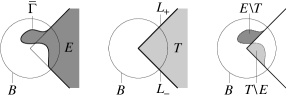
Figure 2.

The rest of this section is devoted to the proofs of Propositions 4.5 and 4.8. The key step is contained in Lemma 4.11 below.

4.10. Potential of a velocity field.

Let $u:\mathbb{R}^{2}\to\mathbb{R}^{2}$ be a continuous velocity field and let $\varphi:\mathbb{R}^{2}\to\mathbb{R}$ be a function of class $C^{1}$. We say that $\varphi$ is a potential for $u$ if

$$u=\nabla^{\perp}\varphi\,,$$

where $\nabla^{\perp}:=(-\partial_{2},\partial_{1})$. Note that $u$ admits a potential if and only if it is divergence-free. In the fluid dynamics literature, such $\varphi$ is called a stream function for the flow generated by $u$.

4.11. Lemma.

Let $\Gamma$ be a given curve, $v$ be a given function on $\Gamma$, both of class $C^{k}$ with $k\geq 2$, and $\bar{r}$ a positive number. Assume that the support of $v$ is contained in a compact (not necessarily proper) sub-arc $G$ of $\Gamma$ and that

$$\int_{\Gamma}v\,d\sigma=0\,.$$ (4.11)

Then there exists a divergence-free, autonomous velocity field $u$ on $\mathbb{R}^{2}$ of class $C^{k-2}$, such that the normal component of $u$ on $\Gamma$, that is, $u\cdot\eta$, agrees with $v$ and such that the support of $u$ is contained in $B(G,\bar{r})$.

• We describe the proof in the case $J=\mathbb{R}$ (recall that $J$ is the domain of the parametrization of the curve $\Gamma$); the case $J=\mathbb{T}^{1}$ requires few straightforward modifications. In view of §4.10, it suffices to find a potential $\varphi:\mathbb{R}^{2}\to\mathbb{R}$ of class $C^{k-1}$ with support contained in $B(G,\bar{r})$, such that

  $$\partial_{\tau}\varphi=v\quad\text{on $\Gamma$,}$$ (4.12)

  where $\tau$ is the tangent vector to $\Gamma$, and then take $u:=-\nabla^{\perp}\varphi$.

  Let $\gamma:\mathbb{R}\to\mathbb{R}^{2}$ be a parametrization of $\Gamma$. For the construction of $\varphi$ we choose:

  • a point $x_{0}=\gamma(s_{0})\in\Gamma$ and, if $G$ is a proper sub-arc of $\Gamma$, we further require that $x_{0}$ does not belong to $G$;

  • a smooth function $g:\mathbb{R}\to\mathbb{R}$ with support contained in $[-1/2,1/2]$ such that $g(0)=1$;

  • a number $r\in(0,\bar{r}]$ strictly smaller than the tubular radius of $\Gamma$.

  Next, we consider the diffeomorphism $\Psi:\mathbb{R}\times(-r,r)\to B(\Gamma,r)$ defined in (4.1), and for every $x=\Psi(s,y)\in B(\Gamma,r)$ we set

  $$\varphi(x)=\varphi(\Psi(s,y)):=g(y/r)\,\int_{s_{0}}^{s}v(\gamma(s^{\prime}))\,|\dot{\gamma}(s^{\prime})|\,ds^{\prime}\,.$$ (4.13)

If $x$ belongs to $\Gamma$, then $x=\gamma(s)=\Psi(s,0)$. Therefore, $\varphi(x)$ is the integral of $v$ along the (oriented) sub-arc of $\Gamma$ starting from $x_{0}$ and ending at $x$, so that the restriction of $\varphi$ to $\Gamma$ is a primitive of $v$ and satisfies (4.12).

Now, Formula (4.13) shows that $\varphi\circ\Psi$ is a function of class $C^{k}$ on $\mathbb{R}\times(-r,r)$ with support contained in $\mathbb{R}\times[-r/2,r/2]$. Since $\Psi$ is a diffeomorphism of class $C^{k-1}$ and maps $\mathbb{R}\times[-r/2,r/2]$ into the closure of $B(\Gamma,r/2)$, we deduce that $\varphi$ is a function of class $C^{k-1}$ on $B(\Gamma,r)$ with support contained in the closure of $B(\Gamma,r/2)$. We complete the construction extending $\varphi$ by $0$ to the complement of this neighborhood in $\mathbb{R}^{2}$.

It remains to check that the support of $\varphi$ is contained in $B(G,\bar{r})$. When ${G=\Gamma}$, this follows from the fact that the support of $\varphi$ is contained in the closure of $B(\Gamma,r/2)$, which in turn is contained in $B(\Gamma,\bar{r})$. When $G=\gamma([s_{1},s_{2}])$ is instead a proper sub-arc of $\Gamma$, we have that:

• $v(\gamma(s))=0$ for $s\notin[s_{1},s_{2}]$ by assumption;

• $s_{0}\notin[s_{1},s_{2}]$ by the choice of $x_{0}$;

• Condition (4.11) can be re-written as $\int_{s_{1}}^{s_{2}}v(\gamma(s^{\prime}))\,|\dot{\gamma}(s^{\prime})|\,ds^{\prime}=0$.

Putting together these facts and recalling the choice of $g$, one easily shows that ${\varphi(\Psi(s,y))=0}$, if $s\notin[s_{1},s_{2}]$ or $y\notin[-r/2,r/2]$, and then

$$\mathrm{supp}(\varphi)\subset\Psi\big{(}[s_{1},s_{2}]\times[-r/2,r/2]\big{)}\subset B(G,\bar{r})\,.\qed$$

• Statement (i) follows from Lemma 4.11, while statement (ii) is an immediate consequence of (i) and §4.7. ∎

• For every $t\in I$, we use Lemma 4.11 to construct a divergence-free velocity field $u(t,\cdot)$ of class $C^{k-2}$, which satisfies the compatibility condition (4.2) at time $t$, and the support of which is contained in $B(G(t),\bar{r}(t))$.

  However, this construction gives only that $u$ is of class $C^{k-2}$ in the variable $x$. To show that $u$ can be taken of class $C^{k-2}$ in $t$ and $x$, we re-examine the proof of Lemma 4.11. The key point in that proof is the regularity of class $C^{k-1}$ in the variables $t,s,y$ of the right-hand side of formula (4.13), which in our specific case is given by

  $$g(y/r(t))\,\int_{s_{0}(t)}^{s}v_{\mathrm{n}}(t,\gamma(t,s^{\prime}))\,|\dot{\gamma}(t,s^{\prime})|\,ds^{\prime}\,.$$

  It is clear that this expression has the required regularity provided that we choose $r(t)$ and $s_{0}(t)$ at least of class $C^{k-1}$ in $t$.

  Since both $\bar{r}(t)$ and the tubular radius of $\Gamma(t)$ are continuous, strictly positive functions of $t$, it is always possible to choose $r(t)$ smaller than both, strictly positive, and smooth in $t$.

  If we only require that the support of $u$ is contained in $B(\Gamma(t),\bar{r}(t))$, we can take $s_{0}(t)$ constant in $t$. If we require that the support of $u$ is contained in ${B(G(t),\bar{r}(t))}$, then we can again choose $s_{0}(t)$ smooth in $t$, but the existence of such a choice is more delicate, and relies on the fact that $G(t)$ is a proper sub-arc for all $t\in I$. ∎

5. First example: pinching

In this section we verify Assumption 3.1 for $s=1$ and for every $1\leq p<\infty$. In fact, we obtain slightly more. We construct a velocity field $u_{0}$ and a solution $\rho_{0}$ of the continuity equation (1.2) on $\mathbb{R}^{2}$, both compactly supported in the open unit square $\mathscr{Q}$, where the velocity has Sobolev regularity $W^{s,p}$, and we do so for each $s$ and $p$ such that $W^{s,p}$ does not embed continuously in the Lipschitz class, that is,

$$s<1 p\leq\infty s\geq 1 p<\frac{2}{s-1}$$ and , or and . (5.1)

This first construction exploits topological changes to the evolution of a certain sets and, therefore, cannot be realized with a Lipschitz velocity field.

More precisely, we give an example of $u_{0}$ and $\rho_{0}$, both defined for $0\leq t\leq 1$, such that:

1. $u_{0}$ is a time-dependent, bounded, and divergence-free velocity field on $\mathbb{R}^{2}$, which is compactly supported on the open unit square $\mathscr{Q}$. The field $u_{0}$ is smooth in both variables $t$ and $x$ for $t\neq k/8$, $k=1,\dots,7$, and bounded in $\dot{W}^{s,p}(\mathbb{R}^{2})$ uniformly in $t$ for $s$ and $p$ in the range (5.1);

2. $\rho_{0}$ is of the form $\rho_{0}(t,\cdot)=1_{E(t)}-\pi/16$, where $E(t)$ is a time-dependent domain in $\mathbb{R}^{2}$ defined for $0\leq t\leq 1$, with the property that its closure is contained in $\mathscr{Q}$ and its area equals $\pi/16$ (thus $\rho_{0}(t,\cdot)$ has average zero). The set $E(t)$ is continuous in $t$, and smooth for $t\neq k/8$, $k=1,\dots,7$;

3. $E(0)$ is the disk with center $0$ and radius $1/4$, while $E(1)$ is the union of the four disks with centers $(\pm 1/4,\pm 1/4)$ and radius $1/8$.

Since $u_{0}$ and $\rho_{0}$ have compact support in the open square $\mathscr{Q}$, we can canonically identify them with fields and functions defined on the torus $\mathbb{T}^{2}$. Remark 2.4(iv) ensures that $u_{0}$ is then bounded in $\dot{W}^{s,p}(\mathbb{T}^{2})$ for the same $s$ and $p$.

Therefore, Assumption 3.1 is satisfied for $s$ and $p$ in the range (5.1), in particular for $s=1$ and for every $1\leq p<\infty$.

Specifically, we construct a time-dependent domain $E$, satisfying the conditions listed above, and a velocity field $u_{0}$ defined for $t\neq k/8$, $k=1,\dots,7$, which is smooth and compatible with $E$. As a consequence, the characteristic function $1_{E(t)}$ is a weak solution of the continuity equation (1.2) in the open time intervals $((k-1)/8,k/8)$, $k=1,\dots,8$. The fact that it is also a solution on the time interval $[0,1]$ is ensured by the continuity in $t$. The set $E(t)$ for $t=k/8$ with $k=0,\dots,4$ and $t=1$ is described in Figure 3.

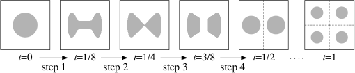
Figure 3. The set $E(t)$ for $t=k/8$ with $k=0,\dots,4$ and $t=1$.

To describe this construction in more details, we denote by $B$ the open disk with center $0$ and radius $1/4$, and by $T$ the cone in $\mathbb{R}^{2}$ such that $|x_{2}|<|x_{1}|$. Next, for $t=1/8$, $t=1/4$, and $t=3/8$ we choose a smooth set $E(t)$ shaped as in Figure 3 making sure that

1. $E(t)$ is symmetric with respect to both axes;

2. $E(t)$ has area $\pi/16$;

3. $E(t)\setminus B$ is the same set at the times $t$ chosen above (i.e., $t=1/8$, $t=1/4$, and $t=3/8$);

4. $(E(1/8)\setminus T)\cap B$ and $(T\setminus E(1/8))\cap B$ have the same area.

In the rest of this section we describe the construction of $E(t)$ and $u_{0}(t,\cdot)$ for $t$ in the time intervals $[0,1/8]$ (Step 1 in Figure 3) and $(1/8,1/4)$ (Step 2 in Figure 3). The construction in the remaining time intervals (steps) is similar, and is omitted.

Step 1: construction of $E(t)$ and $u_{0}(t,\cdot)$ for $0\leq t\leq 1/8$. Since the sets $E(0)$ and $E(1/8)$ are both smooth and have area $\pi/16$, we can clearly find a time-dependent $E(t)$ for $0<t<1/8$ that deforms $E(0)$ to $E(1/8)$ such that $E(t)$ has constant area $\pi/16$ and such that the map $t\mapsto E(t)$ is smooth on $[0,1/8]$. Then, by Proposition 4.5 we can find a smooth velocity field $u_{0}:[0,1/8]\times\mathbb{R}^{2}\to\mathbb{R}^{2}$ that is divergence-free and compatible with $E$. Moreover, since $\partial E(t)$ is contained in $\mathscr{Q}$, we can assume that the support of $u_{0}$ is contained in $\mathscr{Q}$ for all $t$. In particular all positive Sobolev norms of $u_{0}(t,\cdot)$ are uniformly bounded in $t$.

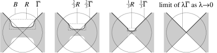
Figure 4. The curve $\smash{\overline{\Gamma}}$, the homothetic copies $\lambda\,\smash{\overline{\Gamma}}$ with $\lambda=2/3$, $\lambda=1/3$, and their limit as $\lambda\to 0$. The circle is centered at $0$ and has radius $1/4$. The set $E(t)$ is in gray.

Step 2: construction of $E(t)$ and $u_{0}(t,\cdot)$ for $1/8<t<1/4$. Let $\smash{\overline{\Gamma}}$ be the proper curve drawn in Figure 4. More precisely, $\smash{\overline{\Gamma}}$ is defined outside $B$ by the equation $x_{2}=|x_{1}|$, and agrees in $B$ with the connected component of the boundary $\partial E(1/8)\cap B$ that lies in the upper half plane.

We pick a smooth decreasing function $\lambda$ on $[1/8,1/4)$ such that $\lambda(1/8)=1$ and $\lambda(t)$ tends to $0$ as $t\to 1/4$. The function $\lambda$ will be explicitly defined later in order to satisfy further requirements.

Then we select the sets $E(t)$, $1/8<t<1/4$, satisfying the following requirements in addition to preserving area and smoothness in time:

1. $E(t)$ agrees with $E(1/8)$ outside $B$;

2. $\partial E(t)\cap B$ has two connected components, which are symmetric with respect to both axes, and the component that lies in the upper half plane agrees with $\lambda(t)\,\smash{\overline{\Gamma}}$ in $B$ (the set $E(t)$ is drawn in gray in Figure 4 for $\lambda(t)=1$, $\lambda(t)=2/3$, and $\lambda(t)=1/3$).

By Remark 4.9(iii), Property (g) above implies that the curve $\smash{\overline{\Gamma}}$ satisfies (4.10) and, therefore, we can apply Proposition 4.8(ii), to obtain a smooth, divergence-free velocity field $w:[1/8,1/4)\times\mathbb{R}^{2}\to\mathbb{R}^{2}$ that is compatible with the homothetic curve $\lambda(t)\,\smash{\overline{\Gamma}}$. Moreover, $w(t,\cdot)$ is compactly supported in the upper half-plane $\mathbb{R}\times(0,+\infty)$ for all $t$ (specifically, we can require that the support is contained in the dashed rectangle $R$ in Figure 4).

Finally, we take $u_{0}:[1/8,1/4)\times\mathbb{R}^{2}\to\mathbb{R}^{2}$ equal to $w$ in the upper half-plane, and we extend it to the lower half-plane by reflection. In this way, $u_{0}$ is still smooth and compactly supported, and by Property (i) above it is compatible with the time-dependent domain $E$ inside the ball $B$. On the other hand, $u_{0}$ vanishes outside the ball $B$ and, therefore, is compatible with the set $E\setminus B$, which is constant in time (recall again Property (g)). In conclusion, $u_{0}$ is compatible with $E$.

It remains to choose $\lambda$ so that $u_{0}(t,\cdot)$ is bounded in $\dot{W}^{s,p}(\mathbb{R}^{2})$ uniformly in $t\in[1/8,1/4)$ for every $s,p$ as in (5.1).To this end, we recall that by Proposition 4.8(ii), the field $u_{0}$ can be written in the form

$$u_{0}(t,x)=\lambda^{\prime}(t)\,\bar{u}\big{(}x/\lambda(t)\big{)},$$

where $\bar{u}:\mathbb{R}^{2}\to\mathbb{R}^{2}$ is smooth and compactly supported. Therefore, using (2.9), for every $t$ we have

$$\|u_{0}(t,\cdot)\|_{\dot{W}^{s,p}(\mathbb{R}^{2})}=|\lambda^{\prime}(t)|\,|\lambda(t)|^{2/p-s}\|\bar{u}\|_{\dot{W}^{s,p}(\mathbb{R}^{2})}\,.$$

Now, a simple computation shows that $u_{0}(t,\cdot)$ is bounded in $\dot{W}^{s,p}(\mathbb{R}^{2})$ uniformly in time for all $s$ and $p$ as in (5.1) if we take

$$\lambda(t):=\exp\Big{(}2-\frac{1}{1-4t}\Big{)}\,.$$

In particular $u_{0}$ is a bounded function in both space and time.

5.1. Remark.

1. The flow of the (non-Lipschitz) velocity field $u_{0}$ changes the topology of sets: the ball at time $t=0$ is transformed into two balls at time ${t=1/2}$.

2. Using symmetry considerations, it is possible to check that the flow of $u_{0}$ compresses a vertical segment to a point, namely the origin (the center of the circle in Figure 4), from time $t=1/8$ to time $t=1/4$. Similarly, the flow of $u_{0}$ expands a point, the origin, to a horizontal segment from time $t=1/4$ to time $t=3/8$.

3. In particular, non-uniqueness holds for the characteristic curves of the velocity field $u_{0}$ starting at any point laying on the vertical segment referenced in point (ii) above at time $t=1/8$.

6. Scaling analysis in a quasi-self-similar construction

As already noted, any velocity field with properties similar to those of the field constructed in Section 5 cannot have Lipschitz regularity, since sets evolved in time by the associated flow do not preserve their connectivity. Indeed, it is not evident how to build an example that satisfies Assumption 3.1 in the case when $s=1$ and $p=\infty$. In this section, we address this case by replacing the (exactly) self-similar scheme of Section 3 with a quasi-self-similar scheme. That is, instead of replicating rescaled copies of one basic element at each step of the evolution (as in §3.3), we consider a finite family of basic elements, which are rescaled and rearranged at each step of the evolution according to a certain combinatorial pattern.

For the quasi-self-similar scheme, we work on the full plane $\mathbb{R}^{2}$. We implement this construction and produce a concrete example in Section 8.

Given $s>0$ and $1\leq p\leq\infty$, Assumption 3.1 is replaced by the assumption below, where we denote by $\lceil s\rceil$ the smallest integer greater or equal than $s$. We recall that $\dot{W}^{s,\infty}$ is the Lipschitz-Hölder space defined in §2.5.

6.1. Assumption: basic family.

There exists an integer $N$ such that, for $j=1,\ldots,N$, there are velocity fields $u_{j}$ and corresponding (not identically zero) solutions $\rho_{j}$ to (1.2), all defined for $0\leq t\leq 1$ and $x\in\mathbb{R}^{2}$, satisfying:

1. each velocity field $u_{j}$ is bounded, divergence-free, tangent to the boundary of the square $\mathscr{Q}$, and bounded in $\dot{W}^{\lceil s\rceil,p}(\mathbb{R}^{2})$ uniformly in time;

2. each solution $\rho_{j}$ is a bounded function and has zero average on $\mathscr{Q}$ for all times;

3. there exists a positive constant $\lambda$, with $1/\lambda$ an integer greater or equal than $2$, such that each function $\rho_{j}(1,\cdot)$ agrees on each square of the tiling $\mathcal{T}_{\lambda}$ (introduced in Definition 3.2) with one of the functions $\rho_{i}(0,\cdot)$ with $1\leq i\leq N$ after rescaling and a possible translation, that is, for each $Q\in\mathcal{T}_{\lambda}$ and for all $x\in Q$,

   $$\rho_{j}(1,x)=\rho_{i(j,Q)}\left(0,\frac{x-r_{Q}}{\lambda}\right)\,,$$

   for a suitable $i=i(j,Q)\in\{1,\ldots,N\}$ and for some point $r_{Q}=r_{Q}(j)$.

We remark that we do not assume that the supports of $u_{j}$ and $\rho_{j}$ are contained in the closure of $\mathscr{Q}$.

6.2. Quasi-self-similar construction.

Under Assumption 6.1, we now define inductively a quasi-self-similar scheme that will be used to give our second, Lipschitz-continuous, example of optimal mixer.

Initial step. We start by choosing a positive constant $\bar{\lambda}$, with $1/\bar{\lambda}$ an integer greater or equal than $1$. We define the evolution for $0\leq t\leq 1$ by patching together velocity fields and solutions on the tiling $\mathcal{T}_{\bar{\lambda}}$ of $\mathscr{Q}$.

For every $Q\in\mathcal{T}_{\bar{\lambda}}$, we select an index $\bar{\jmath}(Q)\in\{1,\ldots,N\}$ and we set for $x\in Q$ and $0\leq t\leq 1$:

$$u(t,x):=\bar{\lambda}\,u_{\bar{\jmath}(Q)}\left(t,\frac{x-r_{Q}}{\bar{\lambda}}\right)\,,\quad\rho(t,x):=\rho_{\bar{\jmath}(Q)}\left(t,\frac{x-r_{Q}}{\bar{\lambda}}\right)\,.$$ (6.1)

For $x\not\in\mathscr{Q}$, we set both $u$ and $\rho$ equal to zero.

We stress that, in this step (as well as in the iterative step below), the resulting field is divergence-free, but it does not necessarily have Sobolev regularity, since the derivative may jump at the boundary of the patch. In what follows, we will temporarily assume the needed regularity (see Assumption 6.3 below), and show afterwards that it is, in fact, fulfilled for the specific example in Section 8.

Since by construction the velocity field $u$ in (6.1) is tangent to the boundary of all the tiles in $\mathcal{T}_{\bar{\lambda}}$, it follows that, for $0<t\leq 1$, the function $\rho$ in (6.1) is a weak solution of the continuity equation with velocity field $u$ globally in $\mathbb{R}^{2}$. We also note that, by Assumption 6.1(iii), the solution at time $1$, $\rho(1,\cdot)$, agrees on each element of the tiling $\mathcal{T}_{\bar{\lambda}}$ with one of the functions $\rho_{i}(0,\cdot)$ after rescaling and possible translation.

Iterative step. For a given positive parameter $\tau$ (to be chosen later), we define

$$T_{n}:=\sum_{i=0}^{n-1}\tau^{i}\quad\text{for $n=1,2,\ldots,\infty$.}$$

We next inductively assume that $u$ and $\rho$ have been defined for $0\leq t\leq T_{n}$, in such a way that on each square of the tiling $\mathcal{T}_{\bar{\lambda}\lambda^{n}}$ the function $\rho(T_{n},\cdot)$ agrees with a rescaled translation of one of the functions $\rho_{i}(0,\cdot)$. We then show how to define $u$ and $\rho$ for $T_{n}<t\leq T_{n+1}$.

We consider a square $Q\in\mathcal{T}_{\bar{\lambda}\lambda^{n}}$. By the inductive assumption, there exists an index $j=j(n,Q)$ such that

$$\rho(T_{n},x)=\rho_{j}\left(0,\frac{x-r_{Q}}{\bar{\lambda}\lambda^{n}}\right)\quad\text{for $x\in Q$.}$$ (6.2)

Accordingly, for $x\in Q$ and $T_{n}<t\leq T_{n+1}$ we define

$$u(t,x):=\frac{\bar{\lambda}\lambda^{n}}{\tau^{n}}u_{j}\left(\frac{t-T_{n}}{\tau^{n}},\frac{x-r_{Q}}{\bar{\lambda}\lambda^{n}}\right)\,,\quad\rho(t,x):=\rho_{j}\left(\frac{t-T_{n}}{\tau^{n}},\frac{x-r_{Q}}{\bar{\lambda}\lambda^{n}}\right)\,.$$ (6.3)

As before, for $x\not\in\mathscr{Q}$ we set both $u$ and $\rho$ equal to zero. By the same argument as in the initial step, we have that, for $T_{n}<t\leq T_{n+1}$, the function $\rho$ in (6.3) is a weak solution of the continuity equation with velocity field $u$ globally in $\mathbb{R}^{2}$.

Again by Assumption 6.1(iii), on each square of the tiling $\mathcal{T}_{\bar{\lambda}\lambda^{n+1}}$ the function $\rho(T_{n+1},\cdot)$ agrees with a rescaled translation of one of the functions $\rho_{i}(0,\cdot)$. This concludes the inductive procedure, which gives a velocity field $u$ and a weak solution $\rho$ of (1.2) defined for a.e. $x\in\mathbb{R}^{2}$ and for all $0\leq t<T_{\infty}$.

We now make a further assumption on the velocity field $u$ obtained by the quasi-self-similar scheme that we have described. One drawback of our construction is, in fact, that we do not a priori control the behavior of derivatives of the field at the boundary of each patch. We are therefore forced at this stage to make a further assumption on $u$, concerning its regularity.

6.3. Assumption: regularity of the patching.

The velocity field $u(t,\cdot)$ belongs to $\dot{W}^{\lceil s\rceil,p}(\mathbb{R}^{2})$ for all $0\leq t<T_{\infty}$.

A few remarks on this delicate point are in order.

6.4. Remark.

1. The fact that Assumptions 6.1 and 6.3 entail regularity of order $\lceil s\rceil$ (rather than $s$) is technical and due to the fact that the norm in a Sobolev space with integer order is local, a property that we will exploit in the proof of Lemma 6.5.

2. Assumption 6.3 is, in fact, the key structural condition to ensure that a quasi-self-similar construction yields velocity fields with the required regularity, as already observed above. It is indeed easy to construct families of velocity fields and solutions that satisfy Assumption 6.1, but not Assumption 6.3.

3. In the relevant case $s=1$ and $p=\infty$, i.e., in the Lipschitz case, Assumption 6.3 is equivalent to assume that $u$ has a continuous representative on $\mathbb{R}^{2}$. In fact, it is sufficient to assume the continuity of $u$ across the boundary of adjacent squares in each tiling.

We stress that in Assumption 6.3, we do not require the Sobolev norm of $u$ to be bounded uniformly with respect to time. The uniformity of the Sobolev bounds in time is then guaranteed by the following lemma.

6.5. Lemma.

Let $\tau=\lambda^{1-s}$. Under Assumptions 6.1 and 6.3, the velocity field $u$ constructed by the quasi-self-similar procedure in §6.2 is divergence-free and is bounded in $\dot{W}^{s,p}(\mathbb{R}^{2})$ uniformly in time.

• First of all, since each velocity field $u_{j}$ is divergence-free in $\mathscr{Q}$ and tangent to the boundary $\partial\mathscr{Q}$, it follows that $u$ is globally divergence-free. It remains to prove the bound on the $\dot{W}^{s,p}(\mathbb{R}^{2})$ norm.

  Step 1: the case $s=k$ an integer. Let $T_{n}<t\leq T_{n+1}$ for some $n\in\mathbb{N}$. Then $u(t,\cdot)$ is defined as in (6.3) for some function $j=j(n,Q)$. Assumption 6.3 guarantees that the $\dot{W}^{k,p}(\mathbb{R}^{2})$ norm of $u(t,\cdot)$ is finite, therefore we only need to estimate the sum of the $\dot{W}^{k,p}$ norms of the restriction of $u(t,\cdot)$ to the squares $Q$ in $\mathcal{T}_{\bar{\lambda}\lambda^{n}}$:

  $$\|u(t,\cdot)\|_{\dot{W}^{k,p}(\mathbb{R}^{2})}^{p} =\int_{\mathscr{Q}}|\nabla^{k}u(t,x)|^{p}\,dx$$

  $$=\sum_{Q\in\mathcal{T}_{\bar{\lambda}\lambda^{n}}}\int_{Q}\left|\nabla^{k}\left(\frac{\bar{\lambda}\lambda^{n}}{\tau^{n}}\,u_{j}\left(\frac{t-T_{n}}{\tau^{n}},\frac{x-r_{Q}}{\bar{\lambda}\lambda^{n}}\right)\right)\right|^{p}\,dx$$

  $$=\sum_{Q\in\mathcal{T}_{\bar{\lambda}\lambda^{n}}}\int_{Q}\left|\frac{\bar{\lambda}\lambda^{n}}{\tau^{n}\bar{\lambda}^{k}\lambda^{kn}}\left(\nabla^{k}u_{j}\right)\left(\frac{t-T_{n}}{\tau^{n}},\frac{x-r_{Q}}{\bar{\lambda}\lambda^{n}}\right)\right|^{p}\,dx$$

  $$=\left(\frac{\lambda^{1-k}}{\tau}\right)^{pn}\bar{\lambda}^{p(1-k)}\sum_{Q\in\mathcal{T}_{\bar{\lambda}\lambda^{n}}}\int_{\mathscr{Q}}\left|\left(\nabla^{k}u_{j}\right)\left(\frac{t-T_{n}}{\tau^{n}},y\right)\right|^{p}(\bar{\lambda}\lambda^{n})^{2}\,dy$$

  $$\leq\left(\frac{\lambda^{1-k}}{\tau}\right)^{pn}\bar{\lambda}^{p(1-k)}\max_{1\leq j\leq N}\sup_{0\leq r\leq 1}\|u_{j}(r,\cdot)\|_{\dot{W}^{k,p}(\mathbb{R}^{2})}^{p}\,.$$

  The computation for $p=\infty$ is similar and gives

  $$\|u(t,\cdot)\|_{\dot{W}^{k,\infty}(\mathbb{R}^{2})}\leq\left(\frac{\lambda^{1-k}}{\tau}\right)^{n}\bar{\lambda}^{(1-k)}\max_{1\leq j\leq N}\sup_{0\leq r\leq 1}\|u_{j}(r,\cdot)\|_{\dot{W}^{k,\infty}(\mathbb{R}^{2})}\,.$$

  The fact that $\tau=\lambda^{1-s}$ gives the desired bound and concludes the proof for $s=k$ integer.

  Step 2: the general case $s\geq 0$ and real. We rely on the previous step and we use (2.11) with $s_{1}=0$, $s_{2}=\lceil s\rceil$ and $\vartheta=1-s/\lceil s\rceil$, obtaining

  $$\|u(t,\cdot)\|_{\dot{W}^{s,p}(\mathbb{R}^{2})} \leq\|u(t,\cdot)\|^{\vartheta}_{L^{p}(\mathbb{R}^{2})}\,\|u(t,\cdot)\|^{1-\vartheta}_{\dot{W}^{\lceil s\rceil,p}(\mathbb{R}^{2})}$$

  $$\leq\left(\frac{\lambda}{\tau}\right)^{\vartheta n}\bar{\lambda}^{\vartheta}\left(\frac{\lambda^{1-\lceil s\rceil}}{\tau}\right)^{(1-\vartheta)n}\bar{\lambda}^{(1-\lceil s\rceil)(1-\vartheta)}\,M_{s,p}$$

  $$=\left(\frac{\lambda^{1-s}}{\tau}\right)^{n}\bar{\lambda}^{1-s}\,M_{s,p}\,,$$

  where

  $$M_{s,p}:=\max_{1\leq j\leq N}\sup_{0\leq t\leq 1}\left[\|u_{j}(t,\cdot)\|_{L^{p}(\mathbb{R}^{2})}+\|u_{j}(t,\cdot)\|_{\dot{W}^{\lceil s\rceil,p}(\mathbb{R}^{2})}\right]\,,$$

  Above we have used the estimate in Step 1 for $k=0$ and $k=\lceil s\rceil$.

  Again, the choice $\tau=\lambda^{1-s}$ allows to conclude. ∎

6.6. Decay of the functional mixing scale.

We now analyze the behavior in time of negative Sobolev norms of the solution $\rho$ constructed in §6.2. For ${T_{n}\leq t<T_{n+1}}$ we have

$$\rho(t,x)=\sum_{Q\in\mathcal{T}_{\bar{\lambda}\lambda^{n}}}\rho_{j}\left(\frac{t-T_{n}}{\tau^{n}},\frac{x-r_{Q}}{\bar{\lambda}\lambda^{n}}\right)\,1_{Q}(x)\quad\text{for $x\in\mathbb{R}^{2}$,}$$

for a suitable $j=j(n,Q)$. For any $r>0$, Equation (2.9) implies that

$$\|\rho(t,\cdot)\|_{\dot{H}^{-r}(\mathbb{R}^{2})} \leq\sum_{Q\in\mathcal{T}_{\bar{\lambda}\lambda^{n}}}\left\|\rho_{j}\left(\frac{t-T_{n}}{\tau^{n}},\frac{x-r_{Q}}{\bar{\lambda}\lambda^{n}}\right)\,1_{Q}(x)\right\|_{\dot{H}^{-r}(\mathbb{R}^{2})}$$

$$=\sum_{Q\in\mathcal{T}_{\bar{\lambda}\lambda^{n}}}\bar{\lambda}^{1+r}\lambda^{n(1+r)}\left\|\rho_{j}\left(\frac{t-T_{n}}{\tau^{n}},\cdot\right)\,1_{\mathscr{Q}}\right\|_{\dot{H}^{-r}(\mathbb{R}^{2})}$$

$$\leq\frac{\bar{\lambda}^{1+r}\lambda^{n(1+r)}}{\bar{\lambda}^{2}\lambda^{2n}}M_{r}=\bar{\lambda}^{r-1}\big{(}\lambda^{r-1}\big{)}^{n}M_{r}\,,$$ (6.4)

with $M_{r}$ defined (for all $r\geq 0$) as

$$M_{r}:=\max_{j=1,\ldots,N}\sup_{0\leq t\leq 1}\|\rho_{j}(t,\cdot)\,1_{\mathscr{Q}}\|_{\dot{H}^{-r}(\mathbb{R}^{2})}\,.$$ (6.5)

Since each $\rho_{j}$ is bounded and has zero average on $\mathscr{Q}$, Remark 2.2(iii) implies that $M_{r}$ is finite for $0\leq r<2$.

Estimate (6.4) gives the correct decay of the homogeneous norms $\dot{H}^{-r}(\mathbb{R}^{2})$ for all $1<r<2$, since in this case $\lambda^{r-1}<1$ and $M_{r}<\infty$. In order to prove the decay of the homogeneous norm $\dot{H}^{-1}(\mathbb{R}^{2})$ we need an interpolation argument. Using (2.10) we find that, for $1<r<2$,

$$\|\rho(t,\cdot)\|_{\dot{H}^{-1}(\mathbb{R}^{2})}\leq\|\rho(t,\cdot)\|^{1/r}_{\dot{H}^{-r}(\mathbb{R}^{2})}\|\rho(t,\cdot)\|^{1-1/r}_{L^{2}(\mathbb{R}^{2})}\,.$$

Together with (6.4), this estimates gives, for $T_{n}\leq t<T_{n+1}$,

$$\|\rho(t,\cdot)\|_{\dot{H}^{-1}(\mathbb{R}^{2})}\leq\bar{\lambda}^{1-1/r}M_{0}^{1-1/r}M_{r}^{1/r}\big{(}\lambda^{1-1/r}\big{)}^{n}\,.$$ (6.6)

Setting

$$c_{r}:=1-1/r>0\,,\quad C_{r}:=\bar{\lambda}^{1-1/r}M_{0}^{1-1/r}M_{r}^{1/r}>0\,,$$

we obtain from (6.6) that, for $T_{n}\leq t<T_{n+1}$,

$$\|\rho(t,\cdot)\|_{\dot{H}^{-1}(\mathbb{R}^{2})}\leq C_{r}\big{(}\lambda^{c_{r}}\big{)}^{n}\,.$$ (6.7)

In particular, choosing $r=3/2$ yields

$$\|\rho(t,\cdot)\|_{\dot{H}^{-1}(\mathbb{R}^{2})}\leq\bar{\lambda}^{1/3}M^{1/3}_{0}M^{2/3}_{3/2}\;\big{(}\lambda^{1/3}\big{)}^{n}\quad\text{for $T_{n}\leq t<T_{n+1}$.}$$ (6.8)

Estimates (6.7) and (6.8) above correspond to (3.4) in §3.3. Therefore, arguing as in the final step of the proof of Theorem 3.4, we obtain the following result.

6.7. Theorem.

Given $s>0$ and $1\leq p\leq\infty$, under Assumptions 6.1 and 6.3, there exist a bounded, divergence-free velocity field $u$ and a solution $\rho$ of the Cauchy problem for (1.2) in $\mathbb{R}^{2}$, such that $u$ is bounded in $\dot{W}^{s,p}(\mathbb{R}^{2})$ uniformly in time, $u$ and $\rho$ are supported in $\mathscr{Q}$ for all times, and the functional mixing scale of $\rho$ exhibits the following behavior:

• case $s<1$: perfect mixing in finite time;

• case $s=1$: exponential decay;

• case $s>1$: polynomial decay.

6.8. Remark.

1. Thanks to Lemma 3.5 we can deduce that the geometric mixing scale of $\rho(t,\cdot)$ exhibits the same behavior as the functional mixing scale.

2. In view of Remark 2.4(iv), the fact that the velocity field and the solution are supported in $\mathscr{Q}$ implies the validity of Theorem 6.7 on the torus $\mathbb{T}^{2}$.

3. For later use (in the companion paper [4]), we make here and in (iv) below some additional observations. In the case $s=1$, every $\dot{H}^{-r}$ norm of $\rho$ decays exponentially in time for $0<r<2$. Moreover,if $M_{\tilde{r}}$ (defined in (6.5)) is finite for some $\tilde{r}\geq 2$, then the $\dot{H}^{-r}$ norm of $\rho$ decays exponentially in time for $0<r<\tilde{r}$.

4. In Section 8 we will verify Assumptions 6.1 and 6.3 for any $s$ and $p$ and construct a velocity field $u$ and a solution $\rho$ that are actually smooth in both time and space. As a consequence of Theorem 6.7, this velocity field is bounded in $\dot{W}^{1,p}(\mathbb{R}^{2})$ uniformly in time and the functional mixing scale of $\rho$ decays exponentially. Additionally, this velocity field satisfies

   $$\|u(t,\cdot)\|_{\dot{W}^{r,p}(\mathbb{R}^{2})}\leq C_{r}\left(\lambda^{1-r}\right)^{t}\,,$$

   for any real number $r\geq 0$. The estimate above follows from the proof of Lemma 6.5 (recalling that in this case $\tau=1$). In particular, the Sobolev norms of $u$ of order higher than one grow exponentially in time, while the Sobolev norms of order lower than one decay exponentially in time.

5. Finally, a reparametrization of the time variable in the example constructed in Section 8 gives a bounded, compactly supported, divergence-free velocity field $u$ such that $u(t,\cdot)\in{\rm Lip}(\mathbb{R}^{2})$ for almost every $0\leq t\leq 1$, and such that the Cauchy problem for the continuity equation associated to this velocity field admits non-unique solutions. Indeed, its Lipschitz norm blows up as $t\downarrow 0$ in such a way that the velocity field fails to belong to $L^{1}([0,1];{\rm Lip}(\mathbb{R}^{2}))$. This example improves on the result in [21] in the $BV$ case (see also [15], [37]).

7. Second geometric construction

In this section we describe another geometric construction of divergence-free velocity fields $u$ together with (non-trivial) solutions $\rho$ of the continuity equation (1.2). The main improvement obtained by this approach is that we construct solutions that are smooth. For paths and curves we follow the notation introduced in Section 4.

We begin with a simple remark. Let $I$ be an open time interval and $D$ an open subset of $\mathbb{R}^{2}$, and let $\{\Phi(t,\cdot):\,t\in I\}$ be an area-preserving flow on $D$ of class $C^{k}$ with $k\geq 2$. In other words, $\Phi:I\times D\to\mathbb{R}^{2}$ is a map of class $C^{k}$ such that, for every $t\in I$, $\Phi(t,\cdot)$ is diffeomorphism from $D$ onto an open set $\Omega(t)$, which satisfies

$$J\Phi(t,z):=\det(\nabla\Phi(t,z))=1.$$

We denote by $\Omega$ the (open) set of all points $(t,x)$ with $t\in I$ and $x\in\Omega(t)$. is then well known that the velocity field $w:\Omega\to\mathbb{R}^{2}$ defined by

$$w(t,x):=\partial_{t}\Phi(t,z)\quad\text{with }x=\Phi(t,z)$$ (7.1)

is of class $C^{k-1}$ and divergence-free.

Moreover, given a bounded function $\bar{\rho}$ on $D$, the function $\rho:\Omega\to\mathbb{R}$ obtained by transporting $\bar{\rho}$ with the flow $\Phi$, that is,

$$\rho(t,x):=\bar{\rho}(z)\quad\text{with }x=\Phi(t,z)\,,$$

is a weak solution of the transport equation (1.1) (which agrees with the continuity equation (1.2), since the velocity is divergence-free).

In the next proposition, we extend this result in order to obtain a velocity field and a solution defined on $I\times\mathbb{R}^{2}$, rather than on $\Omega$.

7.1. Proposition.

Let $D$ be a simply-connected domain in $\mathbb{R}^{2}$, and let $\Phi$ be an area-preserving flow on $D$ of class $C^{k}$, $k\geq 2$. Let $D^{\prime}$ be a closed subset of $D$. Then there exists a divergence-free velocity field $u:I\times\mathbb{R}^{2}\to\mathbb{R}^{2}$ of class $C^{k-1}$ such that

$$u(t,x)=w(t,x)=\partial_{t}\Phi(t,z),\quad\text{if $x=\Phi(t,z)$ for some $z\in D^{\prime}$.}$$ (7.2)

Given $\bar{\rho}:D^{\prime}\to\mathbb{R}$ bounded, the function $\rho:I\times\mathbb{R}^{2}\to\mathbb{R}$ defined by

$$\rho(t,x):=\begin{cases}\bar{\rho}(z)&\text{if $x=\Phi(t,z)$ for some $z\in D^{\prime}$,}\\ 0&\text{otherwise,}\end{cases}$$ (7.3)

is a weak solution of the continuity equation (1.2).

7.2. Remark.

The assumption that $D$ is simply connected can be weakened, but not entirely removed. Indeed, take $D:=\mathbb{R}^{2}\setminus\{0\}$ and let $\{\Phi(t,\cdot):\,t\geq 0\}$ be the flow on $D$ associated with the (autonomous) velocity field $w(x):=x/|x|^{2}$. Since $w$ is divergence-free on $D$, the flow is area preserving. Consider now a curve $\Gamma$ that winds around the origin once counterclockwise. Then the flux through $\Gamma$ of any divergence-free velocity field $u$ defined on $\mathbb{R}^{2}$ must be $0$, while the flux of $w$ is $2\pi$, since the distributional divergence of $w$ on $\mathbb{R}^{2}$ is $2\pi\,\delta_{0}$, where $\delta_{0}$ is the Dirac mass at the origin. This simple example shows that (7.2) cannot hold, if $\Phi(t,D^{\prime})$ contains such a curve $\Gamma$ for some time $t$.

Informally, $u$ is obtained by truncating $w$ on $D^{\prime}$ and extending by zero. The difficulty in doing so is ensuring the divergence-free condition. As customary to circumvent this problem, we truncate instead a potential of $w$. We let $w$ be given by (7.1), and choose a potential $\phi$ for $w$. We then multiply this potential by a suitable cut-off function, which agrees with $1$ on $D^{\prime}$, and define $u$ as the velocity associated to the new potential, which is automatically divergence-free. We now present the proof in detail.

• We begin by selecting a smooth cut-off function $g:\mathbb{R}^{2}\to[0,1]$ that agrees with $1$ on a open neighborhood of $D^{\prime}$ and has support contained in $D$. We choose a point $z_{0}\in D$, which will be used to normalize the potential. Since $D$ is simply connected, $\Omega(t)$ is simply connected for every $t\in I$, and consequently the divergence-free velocity field $w(t,\cdot)$ admits a unique potential $\phi(t,\cdot)$ in the sense of §4.10 that satisfies the normalization condition

  $$\phi(t,x_{0}(t))=0,\quad\text{where}\quad x_{0}(t):=\Phi(t,z_{0})\,.$$ (7.4)

  We then define the truncated potential $\varphi(t,\cdot):\mathbb{R}^{2}\to\mathbb{R}$ by

  $$\varphi(t,x):=\begin{cases}\phi(t,x)\,g(z)&\text{if $x=\Phi(t,z)$ for some $z\in D$, }\\ 0&\text{otherwise,}\end{cases}$$ (7.5)

  and finally take $u:=\nabla^{\perp}\varphi$.

  Since $\Phi$ is of class $C^{k}$, both $w$ and $\phi$ are of class $C^{k-1}$ in both variables, and $\phi$ is of class $C^{k}$ in $x$. Clearly the same holds for $\varphi$, which in turn implies that $u$ is of class $C^{k-1}$. Moreover, $\varphi$ agrees by construction with $\phi$ on an open neighborhood $U$ of the set of all points $\Phi(t,z)$ with $t\in I$, $z\in D^{\prime}$, and therefore $u$ agrees with $w$ on $U$. In particular, (7.2) holds.

  Next, we observe that $\rho$ is obtained by transporting $\bar{\rho}$ with the flow $\Phi$, and hence it solves the continuity equation $\partial_{t}\rho+\mathop{\mathrm{div}}(w\rho)=0$ on $\Omega$. On the other hand, $u$ and $v$ agree on $U$, which contains the support of $\rho$, and therefore $\rho$ solves the continuity equation $\partial_{t}\rho+\mathop{\mathrm{div}}(u\rho)=0$ in $\mathbb{R}^{2}$ as well. ∎

Let $\Gamma$ be a curve in the plane. In the next lemma, we modify the definition of the parametrization $\Psi$ of the tubular neighborhood $B(\Gamma,r)$ given in (4.1), in order to obtain an area-preserving map.

7.3. Lemma.

Let $\Gamma$ be a proper curve parametrized by a path $\gamma:\mathbb{R}\to\mathbb{R}^{2}$ of class $C^{k}$ with $k\geq 3$, such that $|\dot{\gamma}(\cdot)|=\ell$ for some constant $\ell$ and the tubular radius $\bar{r}$ of $\Gamma$ is strictly positive. Let $r$ be a positive number such that $r\leq\ell\bar{r}/2$ and let $\Phi:\mathbb{R}\times(-r,r)\to\mathbb{R}^{2}$ be the map defined by

$$\Phi(s,y):=\gamma(s)+\alpha(s,y/\ell)\,\eta(s)\quad\text{with}\quad\alpha(s,y^{\prime}):=\frac{2y^{\prime}}{1+\sqrt{1-2y^{\prime}\kappa(s)}}\,.$$ (7.6)

Then $\gamma(\cdot)=\Phi(\cdot,0)$ and $\Phi$ is an area-preserving diffeomorphism of class $C^{k-2}$, the image of which is contained in the tubular neighborhood $B(\Gamma,2r/\ell)$ and contains $B(\Gamma,r/(2\ell))$.

• Using the assumption on $r$ and the fact that the tubular radius $\bar{r}$ is no larger than the curvature radius $1/|\kappa|$ of the curve, it follows that $r\leq\ell/(2|\kappa|)$, which implies that $\Phi$ is well defined on $\mathbb{R}\times(-r,r)$.

  We observe that $\alpha$ is a function of class $C^{k-2}$ because $\kappa$ is of class $C^{k-2}$, and that

  $$\Phi(s,y)=\Psi\big{(}s,\alpha(s,y/\ell)\big{)}\quad\text{for every $s,y$,}$$ (7.7)

  where $\Psi$ is defined in (4.1). Since $\Psi$ is a diffeomorphism of class $C^{k-1}$ on $\mathbb{R}\times(-\bar{r},\bar{r})$ and the function $y\mapsto\alpha(s,y/\ell)$ has strictly positive derivative for every $s$ and maps $(-r,r)$ into $(-\bar{r},\bar{r})$, $\Phi$ is a diffeomorphism of class $C^{k-2}$.

  The fact that $\Phi$ is area-preserving, that is, $J\Phi=1$ everywhere, can be verified by a direct computation. For this purpose, it is convenient to write the gradient of $\Phi$ at $(s,y)$ using the canonical basis of $\mathbb{R}^{2}$ for the domain, and the orthonormal basis $\tau(s),\eta(s)$, associated to the foliation of the tubular neighborhood induced by $\Gamma$, for the codomain. This choice gives that

  $$\nabla\Phi(s,y)=\begin{pmatrix}\ell(1+\kappa\,\alpha)&0\\ \partial_{s}\alpha&\frac{1}{\ell}\partial_{y^{\prime}}\alpha\end{pmatrix}\,,$$

  where $\kappa=\kappa(s)$ and $\alpha=\alpha(s,y/\ell)$.

  Finally, the fact that the image of $\Phi$ is contained in $B(\Gamma,2r/\ell)$ and contains $B(\Gamma,r/(2\ell))$ follows from Formula (7.7) and the estimate $r/(2\ell)\leq\alpha\leq 2r/\ell$. ∎

In the next subsections, we associate a velocity field $u$ and a solution $\rho$ of the continuity equation (1.2) to a given time-dependent proper curve $\Gamma$. This construction will provide the building blocks for the example described in the next section.

7.4. Velocity field associated to a time-dependent curve.

Let $\Gamma$ be a time-dependent curve parametrized by a path $\gamma:I\times\mathbb{R}\to\mathbb{R}^{2}$ of class $C^{k}$ with $k\geq 3$. Let $r$ be a positive number such that

1. $|\dot{\gamma}(t,\cdot)|$ is equal to some $\ell(t)>0$ for every $t\in I$;

2. $2r/\ell(t)$ is smaller or equal than the tubular radius of $\Gamma(t)$ for every $t\in I$.

For every $t\in I$ we let $\Phi(t,\cdot)$ be the diffeomorphism on $D:=\mathbb{R}\times(-r,r)$ defined by (7.6), and take the velocity field $u:I\times\mathbb{R}^{2}\to\mathbb{R}^{2}$ as in Proposition 7.1, having set $D^{\prime}:=\mathbb{R}\times[-r/2,r/2]$.

A close inspection of the proof of Proposition 7.1 shows that the construction of $u$ depends on the choice of the point $z_{0}$ in $\mathbb{R}\times(-r,r)$, used in the normalization condition (7.4), and on the choice of the cut-off function $g$. For the construction at hand, we choose:

1. $z_{0}:=(0,0)$;

2. $g(s,y):=\bar{g}(y/r)$, where $\bar{g}:\mathbb{R}\to[0,1]$ is a fixed smooth function that is even, takes value $1$ in a neighborhood of $[-1/2,1/2]$, and its support is contained in $(-1,1)$.

7.5. Canonical solution associated to a time-dependent curve.

We fix an even bounded function $\bar{\rho}:[-1/2,1/2]\to\mathbb{R}$ with zero integral over space and let ${\rho:I\times\mathbb{R}^{2}\to\mathbb{R}}$ be the solution of the continuity equation (1.2) obtained by replacing the function $\bar{\rho}(z)$ in formula (7.3) with $\bar{\rho}(y/r)$, that is,

$$\rho(t,x):=\begin{cases}\bar{\rho}(y/r)&\text{if $x=\Phi(t,s,y)$ for some $s\in\mathbb{R}$, $y\in[-r/2,r/2]$,}\\ 0&\text{otherwise.}\end{cases}$$ (7.8)

7.6. Remark.

1. The velocity field $u$ constructed above is uniquely determined by the choice of the parametrization $\gamma$, the number $r$, and the function $\bar{g}$. Since $\bar{g}$ is fixed for the rest of the paper, the relevant parameters are therefore $\gamma$ and $r$.

2. The solution $\rho$ depends only on purely geometric quantities, and not on the choice of the parametrization $\gamma$. More precisely, using formulas (7.6) and (7.8) one readily checks that the value $\rho(t,x)$ is zero if $\mathrm{dist}(x,\Gamma(t))>r/\ell(t)$, and otherwise it depends on:

   • $r$, $t$, and $\ell(t)$;

   • the distance $\mathrm{dist}(x,\Gamma(t))$;

   • the curvature of $\Gamma(t)$ at the projection of $x$ on $\Gamma(t)$.

3. By construction, for every $t\in I$, the velocity field $u(t,\cdot)$ is supported in $\Phi(t,\mathbb{R}\times(-r,r))$, which is contained in $B(\Gamma(t),2r/\ell(t))$, while $\rho(t,\cdot)$ is supported in $\Phi(t,\mathbb{R}\times(-r/2,r/2))$, which is contained in $B(\Gamma(t),r/\ell(t))$ (cf. Lemma 7.3).

4. It follows from Formula (7.8) that the solution $\rho(t,\cdot)$ has zero integral over space, since the initial data $\bar{\rho}$ is assumed to have the same property and the change of variable $\Phi$ is area preserving. This property will be used in Section 8.

We suppose now that we are given two time-dependent curves $\Gamma$ and $\smash{\widetilde{\Gamma}}$, and we let $u,\tilde{u}$ and $\rho,\tilde{\rho}$ be, respectively, the corresponding velocity fields and solutions constructed in §7.4 and §7.5. In the next section, we will exploit a kind of localization principle, stating that, if $\Gamma$ and $\smash{\widetilde{\Gamma}}$ agree in a neighborhood of some point $x_{0}$, then $u$, $\tilde{u}$ and $\rho$, $\tilde{\rho}$ also agree in a neighborhood of $x_{0}$.

In Lemma 7.8 we give a precise statement of this principle, specifically designed for the applications described in the next section.

We first introduce some additional notation.

7.7. Centered sub-arcs and curved rectangles.

Let $\Gamma$ be a curve parametrized by a path $\gamma$ such that $|\dot{\gamma}(\cdot)|=\ell$ constant, and let $x_{0}=\gamma(s_{0})$ be a point on $\Gamma$. For a given $\delta>0$, we denote by $I(\Gamma,x_{0},\delta)$ the (centered) sub-arc given by all $x\in\Gamma$ such that their geodesic distance from $x_{0}$ is strictly less than $\delta$. That is,

$$I(\Gamma,x_{0},\delta):=\gamma\big{(}(s_{0}-\delta/\ell,s_{0}+\delta/\ell)\big{)}\,.$$

Moreover, given a $\delta^{\prime}>0$ that is no larger than the tubular radius of $\Gamma$, we denote by $R(\Gamma,x_{0},\delta,\delta^{\prime})$ the (open, centered) curved rectangle given by all $x\in\mathbb{R}^{2}$ such that their distance from $\Gamma$ is strictly less than $\delta^{\prime}$ and their projection on $\Gamma$ belongs to $I(\Gamma,x_{0},\delta)$. That is,

$$R(\Gamma,x_{0},\delta,\delta^{\prime}):=\Psi\big{(}(s_{0}-\delta/\ell,s_{0}+\delta/\ell)\times(-\delta^{\prime},\delta^{\prime})\big{)}\,,$$

where again $\Psi$ is defined in (4.1).

7.8. Lemma.

Let $\Gamma$ and $\smash{\widetilde{\Gamma}}$ be two time-dependent, proper curves of class $C^{k}$ with $k\geq 3$, parametrized by $\gamma,\tilde{\gamma}:I\times\mathbb{R}\to\mathbb{R}^{2}$, respectively. Assume that (a) and (b) in §7.4 are verified by $\gamma$ and $\tilde{\gamma}$ with the same $\ell:I\to(0,+\infty)$ and the same $r>0$. Let $u,\tilde{u}$ be defined as in §7.4 and $\rho,\tilde{\rho}$ be defined as in §7.5. Assume in addition that there exist $\delta>0$ and $s_{0}\in\mathbb{R}$ such that, for every $t\in I$,

1. $\gamma(t,s_{0})=\tilde{\gamma}(t,0)=:x_{0}(t)$;

2. the sub-arcs $I\big{(}\Gamma(t),x_{0}(t),\delta\big{)}$ and $I\big{(}\smash{\widetilde{\Gamma}}(t),x_{0}(t),\delta\big{)}$ coincide and have the same orientation;

3. denoting by $v_{\mathrm{n}}$ the normal velocity of $\Gamma$, we have

   $$\int\limits_{\gamma(t,[0,s_{0}])}\hskip-5.0ptv_{\mathrm{n}}(t,x)\,d\sigma(x)=0\,.$$

Then $u(t,x)=\tilde{u}(t,x)$ and $\rho(t,x)=\tilde{\rho}(t,x)$ for every $t\in I$ and every $x$ in the curved rectangle $R(t):=R\big{(}\Gamma(t),x_{0}(t),\delta,2r/\ell(t)\big{)}$.

The proof is not difficult, but we must revisit the entire construction of $u$ and $\rho$, which is divided between §7.4, §7.5, and the proofs of Proposition 7.1 and Lemma 7.3.

• We fix $t\in I$. Using that (a) and (b) are assumed verified, and the fact that $\gamma(t,\cdot)$ and $\tilde{\gamma}(t,\cdot)$ have the same parametrization speed $\ell(t)$, we obtain that

  $$\gamma(t,s+s_{0})=\tilde{\gamma}(t,s),\quad\text{when $|s|\leq\delta/\ell$.}$$

  From this identity, it readily follows that the flows $\Phi$ and $\smash{\widetilde{\Phi}}$ defined by (7.6) satisfy

  $$\Phi(t,s+s_{0},y)=\smash{\widetilde{\Phi}}(t,s,y),\quad\text{when $|s|\leq\delta/\ell$, $|y|<r$,}$$ (7.9)

  which implies that the velocity fields $w$ and $\smash{\widetilde{w}}$ defined by (7.1) satisfy

  $$w(t,x)=\smash{\widetilde{w}}(t,x),\quad\text{when $x\in U(t)$,}$$ (7.10)

  where

  $$U(t):=\big{\{}\smash{\widetilde{\Phi}}(t,s,y)\,:\ |s|\leq\delta/\ell\,,\ |y|<r\big{\}}\,.$$

  We let now $\phi(t,\cdot)$ and $\smash{\widetilde{\phi}}(t,\cdot)$ be the potentials of $w(t,\cdot)$ and $\smash{\widetilde{w}}(t,\cdot)$, respectively, constructed in the proof of Proposition 7.1. We claim that

  $$\phi(t,x)=\smash{\widetilde{\phi}}(t,x)\quad\text{when $x\in U(t)$.}$$ (7.11)

  Since the corresponding fields agree on $U$ and $U$ is connected, it suffices to show that these potentials agree at one point in $U$. We will show that they both vanish at $x_{0}(t)$. Indeed, formula (7.4), Assumption (c) in §7.4, and the identities $\Phi(t,0,0)=\gamma(t,0)$ and $\smash{\widetilde{\Phi}}(t,0,0)=\tilde{\gamma}(t,0)$ yield

  $$\phi\big{(}t,\gamma(t,0)\big{)}=\smash{\widetilde{\phi}}\big{(}t,\tilde{\gamma}(t,0)\big{)}=0\,.$$

  Since $\tilde{\gamma}(t,0)=x_{0}(t)$, it follows that

  $$\tilde{\phi}(t,x_{0}(t))=0\,.$$

  Finally, since $x_{0}(t)=\gamma(t,s_{0})$, taking into account again (c) and the identity $v_{\mathrm{n}}=w\cdot\eta$, we obtain

  $$\phi(t,x_{0}(t))=\phi(t,\gamma(t,s_{0})) =\phi(t,\gamma(t,s_{0}))-\phi(t,\gamma(t,0))$$

  $$=\int\limits_{\gamma(t,[0,s_{0}])}w\cdot\eta\,d\sigma=\int\limits_{\gamma(t,[0,s_{0}])}v_{\mathrm{n}}\,d\sigma=0\,.$$

  The proof of (7.11) is complete.

  The rest of the proof is straightforward. From (7.11) and the choice of the cut-off function $g$ (see (d) in §7.4), we have that the truncated potentials $\varphi(t,\cdot)$ and $\tilde{\varphi}(t,\cdot)$, defined by (7.5), agree on $U(t)$. Furthermore, one can show that both potentials vanish on $R(t)\setminus U(t)$, and therefore they agree on the whole $R(t)$, which implies that the corresponding velocity fields $u(t,\cdot)$ and $\tilde{u}(t,\cdot)$ agree on $R(t)$.

  It remains to show that

  $$\rho(t,x)=\tilde{\rho}(t,x)\quad\text{when $x\in R(t)$,}$$ (7.12)

  but this fact follows from Remark 7.6(ii). ∎

8. Second example: Peano snake

In this final section, we verify Assumptions 6.1 and 6.3 for any $s$ and $p$ and construct a specific example of quasi-self-similar evolution. By doing so, we validate the assumptions of Theorem 6.7. In particular, we establish the existence of a bounded, divergence-free velocity field supported in the unit square, which is Lipschitz continuous uniformly in time, and the existence of a solution of the continuity equation (1.2) with the property that its functional and geometric mixing scales decay exponentially in time. We call this example the “Peano snake”, since the construction is reminiscent of the iterative construction of the Peano curve (cf. Figure 6).

The velocity field and the solution that we construct are smooth in both time and space (see Remark 8.9). However, any Sobolev norm of order higher than one is not bounded uniformly in time.

We proceed as follows. In §8.1, we first describe the combinatorial structure of our example. Using the tools provided in Section 7, we then prove in §8.5, §8.6, and §8.7 that the construction of a basic family verifying Assumptions 6.1 and 6.3 can be reduced to the construction of two time-dependent, proper curves satisfying a certain number of geometric conditions. These conditions are given in §8.2 and §8.3. Finally in §8.10, §8.11, and §8.12, we present the actual construction of the two curves.

8.1. Combinatorial structure.

We begin by illustrating the combinatorial structure of this quasi-self-similar example. The complete construction is rather complex and the purpose of this subsection is to provide a graphical representation of the solution for the first two steps in the iteration, in order to help the reader visualize our construction. We omit all details that are not needed for this purpose.

The starting point is a basic family (in the sense of Assumption 6.1) consisting of six pairs of velocity fields $u_{j}$ and solutions $\rho_{j}$. At this stage, we do not directly define $u_{j}$ and $\rho_{j}$, rather we describe the supports of the solutions $\rho_{j}$, which we denote by $E_{j}$. In fact, we describe the sets $E_{j}$ only for $j=1,2$ and only at the initial time $t=0$ and at the final time $t=1$ (Figure 5). The sets $E_{j}$ for $j=3,\dots,6$ are obtained by means of appropriate rotations.

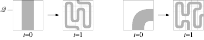
Figure 5. An example of basic family for a quasi-self-similar construction: the sets in gray are the supports $E_{j}$ of the solutions $\rho_{j}$ for $j=1$ (left) and $j=2$ (right) and at times $t=0$ and $t=1$.

As depicted in Figure 5, at time $t=0$ the sets $E_{1}$ and $E_{2}$ are, respectively, a straight strip (Figure 5, left) and a bent strip (Figure 5, right), while at time $t=1$ they are composed by $25$ rotated and translated copies of the two basic elements, scaled by a factor $\lambda=1/5$.

To obtain the velocity $u$ and solution $\rho$, we implement the construction in §6.2 with $\bar{\lambda}=1/2$. In the first step of the construction, we must choose a pair $(u_{j},\rho_{j})$ from the basic family for every square in the tiling $\mathcal{T}_{1/2}$. Our choice is such that at time $t=0$ the corresponding sets $E_{j}$ are all bent strips, and are patched together to create the (almost round) annulus shown in Figure 6, left.

This annulus is the support of the initial data $\bar{\rho}$. Using Figure 5 we can draw the support of the solution $\rho$ at time $t=T_{1}=1$ (Figure 6, middle), then at time $t=T_{2}=1+\tau$ (Figure 6, right), and so on.

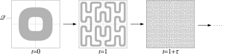
Figure 6. Initial choice of the four basic elements and further steps in the quasi-self-similar evolution: the grayed set is the support of the solution at each step.

While Figures 5 and 6 give an accurate illustration of the combinatorial structure of the example that will be presented in full detail in the rest of this section, a rigorous justification of the example requires a careful analysis, as we need to produce a smooth solution $\rho$ that is transported by a smooth, divergence-free velocity field $u$.

8.2. Conditions on the basic curves.

The fundamental ingredient of our construction will be two time-dependent proper curves $\Gamma_{1}(t)$ and $\Gamma_{2}(t)$, corresponding to the two sets $E_{1}$ and $E_{2}$ described in §8.1, with parametrizations $\gamma_{1}$, $\gamma_{2}:[0,1]\times\mathbb{R}\to\mathbb{R}^{2}$ of class $C^{\infty}$, such that, for every $t\in[0,1]$:

1. $\gamma_{1}(t,0)=\gamma_{2}(t,0)=(0,-1/2)$, $\gamma_{1}(t,1)=(0,1/2)$, and $\gamma_{2}(t,1)=(1/2,0)$;

2. there exists a constant $\delta>0$ such that outside the square $(1-\delta)\mathscr{Q}$, homothetic to $\mathscr{Q}$, each of the curves $\Gamma_{1}(t)$ and $\Gamma_{2}(t)$ agrees with two unbounded half-lines, orthogonal to $\partial\mathscr{Q}$ and passing through the points defined in (a);

3. $|\dot{\gamma}_{1}(t,s)|=|\dot{\gamma}_{2}(t,s)|=:\ell(t)$ for every $s\in\mathbb{R}$, and in particular the intersections of the curves $\Gamma_{1}(t)$ and $\Gamma_{2}(t)$ with $\mathscr{Q}$ have length $\ell(t)$;

4. denoting by $v_{\mathrm{n}}^{1}$ and $v_{\mathrm{n}}^{2}$, the normal velocity of $\Gamma_{1}$ and $\Gamma_{2}$, respectively, then

   $$\int\limits_{\gamma_{1}(t,[0,1])}v_{\mathrm{n}}^{1}(t,x)\,d\sigma(x)=\int\limits_{\gamma_{2}(t,[0,1])}v_{\mathrm{n}}^{2}(t,x)\,d\sigma(x)=0\,;$$

5. for every square $Q$ in the tiling $\mathcal{T}_{1/5}$ of $\mathscr{Q}$, the sub-arc $\Gamma_{1}(1)\cap Q$ can be written as a translated, rescaled, and possibly rotated copy of $\Gamma_{1}(0)\cap\mathscr{Q}$ or $\Gamma_{2}(0)\cap\mathscr{Q}$; the same holds for $\Gamma_{2}(1)\cap Q$.

8.3. Simplified geometric conditions.

In this paragraph we replace some of the conditions in §8.2 by purely geometric ones, that is, conditions that are written in terms of the curves $\Gamma_{1}$ and $\Gamma_{2}$ and do not involve the parametrizations $\gamma_{1}$ and $\gamma_{2}$. In §8.10, §8.11, and §8.12, we will then be able to give the curves $\Gamma_{1}$ and $\Gamma_{2}$ without describing explicitly the parametrizations $\gamma_{1}$ and $\gamma_{2}$.

More precisely, we consider the following alternative conditions, in which we denote by $\ell_{1}(t)$ and $\ell_{2}(t)$ the length of the intersection of the curve $\Gamma_{1}(t)$ and $\Gamma_{2}(t)$ with $\mathscr{Q}$, respectively:

1. $\ell_{1}(0)=\ell_{2}(0)$;

1. the derivatives in $t$ of the functions $\ell_{1}(t)$ and $\ell_{2}(t)$ are strictly positive;

1. the area of both connected components of $\mathscr{Q}\setminus\Gamma_{1}(t)$ equals $1/2$, and the same holds for the area of the two connected components of $\mathscr{Q}\setminus\Gamma_{2}(t)$.

We claim that Conditions (b), (c’), (c”), (d’), and (e) imply Conditions (a)-(e) in §8.2. First of all, (a) follows from (b) by choosing suitable parametrizations $\gamma_{1}(t,\cdot)$ and $\gamma_{2}(t,\cdot)$. Next, we modify such parametrizations in such a way that $|\dot{\gamma}_{1}(t,\cdot)|$ and $|\dot{\gamma}_{2}(t,\cdot)|$ are constant for all $t$. This fact, together with (a), entails that $|\dot{\gamma}_{1}(t,s)|=\ell_{1}(t)$ and $|\dot{\gamma}_{2}(t,s)|=\ell_{2}(t)$. Condition (c’), together with condition (e), implies that $\ell_{1}(1)=\ell_{2}(1)=5\ell_{1}(0)$. Then condition (c”) implies that with a change of variable in $t$ we can achieve $\ell_{1}(t)=\ell_{2}(t)=:\ell(t)$ for all $t$, that is, condition (c) holds. Finally (d) and (d’) are equivalent by Remark 4.6(iii).

8.4. A preliminary example.

Two curves satisfying some, but unfortunately not all, of the conditions in §8.2 are depicted in Figure 7 (to be compared with Figure 5). In this figure we can see the evolution of $\Gamma_{1}$ starting from a straight segment $\Gamma_{1}(0)$ inside $\mathscr{Q}$, and the evolution of $\Gamma_{2}$ starting from a (slightly modified) quarter of circle $\Gamma_{2}(0)$ inside $\mathscr{Q}$. Note that both $\Gamma_{1}(1)$ and $\Gamma_{2}(1)$ can be written as unions of $25$ copies of the segment $\Gamma_{1}(0)$ or of the (modified) quarter of circle $\Gamma_{2}(0)$ which are scaled by a factor $1/5$ and suitably rotated and translated.

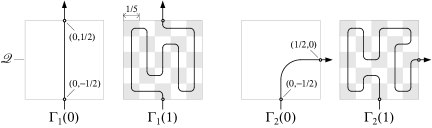
Figure 7. Example of curves satisfying (a), (b), and (e) in §8.2.

From the geometry of $\Gamma_{1}$ and $\Gamma_{2}$ as shown in Figure 7, it follows that these curves satisfy Conditions (a), (b), and (e) (which is the most relevant). However, Condition (c) fails at $t=0$ and $t=1$, while Condition (d) depends on the parametrization and cannot be directly verified from the picture. Moreover, these curves do not satisfy some of the alternative conditions either, namely Conditions (c’) and (d’), while Condition (c”) could be in principle satisfied, at least for some choice of the curves for $0<t<1$.

In §8.10, §8.11, and §8.12 we construct an example of basic curves satisfying the conditions in §8.2 and §8.3. That construction is a modification of the present example (cf. Figure 9) and is significantly more complex.

In the next subsections, we assume the existence of two basic curves $\Gamma_{1}$ and $\Gamma_{2}$ as in §8.2 and §8.3. We then use the results in Section 7 to construct some associated velocity fields $u_{1}$ and $u_{2}$, and solutions $\rho_{1}$ and $\rho_{2}$ that satisfy Assumption 6.1. Next, we obtain the velocity field $u$ and the solution $\rho$ by implementing the iterative procedure in §6.2, according to the combinatorial structure in §8.1. Afterwards, we verify that $u$ satisfies Assumption 6.3. Lastly, we establish additional regularity properties of $u$ and $\rho$.

8.5. Construction of $\boldsymbol{u_{i}}$ and $\boldsymbol{\rho_{i}}$.

We choose a small $r>0$ such that:

• $r<\min\{\frac{1}{2}r_{1}(t)\ell(t),\,\frac{1}{2}r_{2}(t)\ell(t)\}$ for every $t\in[0,1]$, where $r_{1}(t)$ and $r_{2}(t)$ are the tubular radii of $\Gamma_{1}(t)$ and $\Gamma_{2}(t)$, respectively, and $\ell(t)$ is as in §8.2(c);

• $B(\Gamma_{1}(t),2r)\subset\mathscr{Q}$ and $B(\Gamma_{2}(t),2r)\subset\mathscr{Q}$ for every $t\in[0,1]$.

Such an $r$ exists due to the smoothness of $\Gamma_{1}$ and $\Gamma_{2}$, and Condition (b) in §8.2.

Then we follow the steps described in §7.4 and §7.5 to obtain the associated time-dependent divergence-free velocity fields $u_{1}$ and $u_{2}$ of class $C^{\infty}$, and the corresponding smooth solutions $\rho_{1}$ and $\rho_{2}$. One readily checks that:

1. $u_{1}(t,\cdot)$ and $\rho_{1}(t,\cdot)$ are supported in $B(\Gamma_{1}(t),2r/\ell(t))$, while $u_{2}(t,\cdot)$ and $\rho_{2}(t,\cdot)$ are supported in $B(\Gamma_{2}(t),2r/\ell(t))$;

2. in particular, the supports of $u_{1}(t,\cdot)$ and $\rho_{1}(t,\cdot)$ intersect $\partial\mathscr{Q}$ inside the segments $(-\frac{2r}{\ell(t)},\frac{2r}{\ell(t)})\times\{-\frac{1}{2}\}$ and $(-\frac{2r}{\ell(t)},\frac{2r}{\ell(t)})\times\{\frac{1}{2}\}$, while the supports of $u_{2}(t,\cdot)$ and $\rho_{2}(t,\cdot)$ intersect $\partial\mathscr{Q}$ inside the segments $(-\frac{2r}{\ell(t)},\frac{2r}{\ell(t)})\times\{-\frac{1}{2}\}$ and $\{\frac{1}{2}\}\times(-\frac{2r}{\ell(t)},\frac{2r}{\ell(t)})$;

3. $u_{1}(t,\cdot)$ and $u_{2}(t,\cdot)$ are tangent to the boundary $\partial\mathscr{Q}$.

As a matter of fact, Properties (a) and (b) above follow at once from Remark 7.6(iii).

Next we show that $u_{1}$ is tangent to the segment $(-\frac{2r}{\ell(t)},\frac{2r}{\ell(t)})\times\{\frac{1}{2}\}$.

(The rest of Property (c) above can be proved in a similar way.)

We consider the vertical line $\tilde{\Gamma}(t)$ with parametrization $\tilde{\gamma}(t,s)=(0,\frac{1}{2}+s\ell(t))$ and let $\tilde{u}$ be the velocity field associated to $\tilde{\Gamma}$ as in §7.4. We now apply Lemma 7.8 to $\tilde{\Gamma}$ and $\Gamma_{1}$ with $s_{0}=1$ and $x_{0}(t)=(0,\frac{1}{2})$, and we obtain that, for any $t\in[0,1]$, the velocity field $\tilde{u}(t,\cdot)$ coincides with $u_{1}(t,\cdot)$ in the rectangle

$$\textstyle R\big{(}\Gamma_{1}(t),(0,\frac{1}{2}),\delta,\frac{2r}{\ell(t)}\big{)}=\big{(}-\frac{2r}{\ell(t)},\frac{2r}{\ell(t)}\big{)}\times\big{(}\frac{1}{2}-\delta,\frac{1}{2}+\delta\big{)}\,.$$

It is, therefore, sufficient to show that $\tilde{u}(t,\cdot)$ is tangent to $\big{(}-\frac{2r}{\ell(t)},\frac{2r}{\ell(t)}\big{)}\times\{\frac{1}{2}\}$ for any $t\in[0,1]$. This property follows from the fact that the diffeomorphism $\tilde{\Phi}$ in (7.6), associated to $\tilde{\Gamma}$, has the form

$$\tilde{\Phi}(t,y)=\left(\frac{y}{\ell(t)}\,,\,\frac{1}{2}+s\ell(t)\right)\,,$$

and from the construction in §7.4.

8.6. Verification of Assumption 6.1 for $\boldsymbol{u_{i}}$ and $\boldsymbol{\rho_{i}}$.

First, we recall that the velocity fields $u_{1}$ and $u_{2}$ are smooth and tangent to the boundary $\partial\mathscr{Q}$, and in particular satisfy Assumption 6.1(i), while Assumption 6.1(ii) follows from Remark 7.6(iv). Assumption 6.1(iii) can be obtained by combining the fact that the solutions $\rho_{1}$ and $\rho_{2}$ can be described in purely geometric terms (see Remark 7.6(ii)) and the quasi-self-similarity of the curves $\Gamma_{1}$ and $\Gamma_{2}$ in Condition (e) in §8.2.

8.7. Verification of Assumption 6.3 for $\boldsymbol{u}$.

We first observe that, according to the general scheme for a quasi-self similar construction (see §6.2) and to the specific combinatorial structure of our example (see §8.1), for $T_{n}<t\leq T_{n+1}$ and on each of the tiles in $\mathcal{T}_{1/(2\cdot 5^{n})}$, the velocity field $u$ agrees with one of the velocity fields $u_{1}$ and $u_{2}$ constructed in §8.5 after a rescaling, a translation and possible rotation.

We next check that $u$ is smooth on the entire plane $\mathbb{R}^{2}$. This result will imply Assumption 6.3 for any $s$ and $p$. The regularity in the interior of each square of the tiling $\mathcal{T}_{1/(2\cdot 5^{n})}$ follows from the regularity of $u_{1}$ and $u_{2}$. We are, therefore, left with checking the regularity across the boundary of $\mathscr{Q}$ and at the interface between each pair of squares in the tiling.

The combinatorial structure in §8.1 guarantees that, at every time, the rotated and rescaled translations of the curves $\Gamma_{1}$ and $\Gamma_{2}$ never intersect the boundary of $\mathscr{Q}$. Indeed, they always intersect the boundary of a tile that is adjacent to another tile, but never at the boundary of $\mathscr{Q}$. Together with Property (b) in §8.5, this observation implies that the velocity field $u$ vanishes in a neighborhood of the boundary of $\mathscr{Q}$, and therefore is regular there.

It remains to prove the regularity of $u$ at the interface $\Sigma$ between two adjacent squares $Q^{\prime}$ and $Q^{\prime\prime}$ of $\mathcal{T}_{1/(2\cdot 5^{n})}$. We call $\Gamma^{\prime}$ and $\Gamma^{\prime\prime}$ the rotated and rescaled translations of the curves $\Gamma_{1}$ and/or $\Gamma_{2}$ which lie inside $Q^{\prime}$ and $Q^{\prime\prime}$, respectively (see Figure 8). We have two possibilities: either the curves $\Gamma^{\prime}$ and $\Gamma^{\prime\prime}$ do not intersect the interface $\Sigma$, or at least one of them does. In the first case $u$ is zero in a neighborhood of $\Sigma$ (again from Property (b) in §8.5), and therefore there is nothing to prove. In the second case, the combinatorial structure in §8.1 guarantees that both $\Gamma^{\prime}$ and $\Gamma^{\prime\prime}$ intersect $\Sigma$ at its mid point, which we denote by $\tilde{x}$.

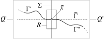
Figure 8.  

Without loss of generality, we can always assume that the segment $\Sigma$ is vertical, as in Figure 8. Then we denote by $\widetilde{\Gamma}$ the horizontal straight line passing through the mid point $\tilde{x}$ of $\Sigma$, parametrized by $\tilde{\gamma}(s):=\tilde{x}+(s,0)$, and by $\tilde{u}$ the (autonomous) velocity field associated to the parametrization $\tilde{\gamma}$ and the positive number $r/5^{n}$ as in §7.4, where $r$ is chosen in §8.5. Moreover, we denote by $R$ the open rectangle centered at $\tilde{x}$ with width $2\delta/5^{n}$ and height $4r$ (see Figure 8 again).

We note that, by construction, the velocity field $u$ agrees in $Q^{\prime}$ (up to a rotation, a translations and rescaling) with one of the basic velocity fields $u_{1}$ and $u_{2}$, and therefore it agrees with the velocity field associated to the parametrization of $\Gamma^{\prime}$ and the number $r/5^{n}$ as in §7.4. Then Condition (d) in §8.2 shows that we can apply Lemma 7.8 and obtain that $u$ and $\tilde{u}$ agree in $R\cap\bar{Q}^{\prime}$. Since the same argument applies to the square $Q^{\prime\prime}$, we have that $u$ and $\tilde{u}$ agree on the whole rectangle $R$. Hence, $u$ is smooth as the restriction of $\tilde{u}$ to $R$.

We conclude the proof of the smoothness of $u$ (across the interface $\Sigma$) by noticing that, again by construction, $u$ vanishes in a neighborhood of the complement in $\Sigma$ of the vertical segment centered at $\tilde{x}$ with height $2r/5^{n}$.

8.8. Regularity in space of $\boldsymbol{\rho}$.

The same procedure just described in §8.7 can be applied to the solution $\rho$, which is therefore smooth on the whole $\mathbb{R}^{2}$ for each time $t$.

8.9. Regularity in time of $\boldsymbol{u}$ and $\boldsymbol{\rho}$.

In §8.7 and §8.8 we have shown that $u$ and $\rho$ are smooth with respect to space. Moreover, they are also smooth in time in each time interval $[T_{n},T_{n+1}]$. This property follows from the regularity with respect to time of the basic curves $\Gamma_{1}(t)$ and $\Gamma_{2}(t)$. We observe that $u$ and $\rho$ may fail to be more regular than continuous in time at $t=T_{n}$. However, we can apply the procedure described in §3.6 to obtain a new velocity field and a new solution that are smooth on $\mathbb{R}^{2}\times[0,T_{\infty})$.

What remains to be done is constructing two time-dependent curves $\Gamma_{1},\Gamma_{2}$ on the time interval $I=[0,1]$ that satisfy Conditions (b), (c’), (c”), (d’), and (e) in §8.2 and §8.3 (and, therefore, also all Conditions (a)-(e)).

Due to the complexity that a rigorous construction would entail, we only give a precise description of the initial states $\Gamma_{1}(0)$, $\Gamma_{2}(0)$, and of the final states $\Gamma_{1}(1)$, $\Gamma_{2}(1)$ (see Figure 9) and sketch some of the intermediate states (see Figures 10, 11, and 12).

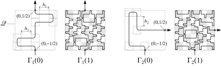
Figure 9. The curves $\Gamma_{1}$ and $\Gamma_{2}$ for $t=0$ and $t=1$.

8.10. Construction of $\boldsymbol{\Gamma_{1}}$ and $\boldsymbol{\Gamma_{2}}$ for $\boldsymbol{t=0,\,t=1}$.

We take $\Gamma_{1}$ and $\Gamma_{2}$ at the initial time $t=0$ and at the final time $t=1$ as in Figure 9. Note that the curves $\Gamma_{1}(0)$ and $\Gamma_{2}(0)$ have been obtained by modifying the curves described in Figure 7 (which, we recall, do not satisfy (c’) and (d’) in §8.3). We specify that:

• all the small squares drawn in the first and third picture in Figure 9 have side-length $1/5$;

• outside these small squares the curves $\Gamma_{1}(0)$ and $\Gamma_{2}(0)$ consists of segments and half-lines;

• the intersections of $\Gamma_{1}(0)$ and $\Gamma_{2}(0)$ with the small squares agree up to reflections, rotations, translations, and scaling by a factor $1/5$ with a fixed curve $\Gamma_{0}$ in the unit square $\mathscr{Q}$; the curve $\Gamma_{0}$ is a “modified quarter of circle” such as, for example, the intersection of the curve $\Gamma_{2}(0)$ in Figure 7 with the unit square $\mathscr{Q}$;

• the parameters $h_{1}$ and $h_{2}$ used in the construction are chosen so that $\Gamma_{1}(0)$ and $\Gamma_{2}(0)$ satisfy  (c’) and (d’) in §8.3; in fact, we first choose $h_{2}$ so that $\Gamma_{2}(0)$ satisfies the equal-area requirement of Condition (d’) (we note that $\Gamma_{1}(0)$ will satisfy this last condition independently of the choice of $h_{1}$ for symmetry reasons), and then we choose $h_{1}$ so that $\Gamma_{1}(0)$ and $\Gamma_{2}(0)$ have the same length in $\mathscr{Q}$, that is, (c’) holds;

• finally, both $\Gamma_{1}(1)$ and $\Gamma_{2}(1)$ consist of $25$ copies of $\Gamma_{1}(0)$ and $\Gamma_{2}(0)$, rotated, reflected, translated, and scaled by a factor $1/5$; thus Condition (e) is met.

8.11. Construction of $\boldsymbol{\Gamma_{1}(t)}$ for $\boldsymbol{0<t<1}$.

The transition from the curve $\Gamma_{1}(0)$ to the curve $\Gamma_{1}(1)$ is given in Figure 10.

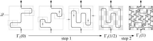
Figure 10. The evolution of $\Gamma_{1}$ from $t=0$ to $t=1$ in two steps.

More precisely, we specify that:

• the small squares drawn in the fourth picture have side-length $1/5$, and within each of these squares, $\Gamma_{1}(1/2)$ agrees with one of the modified quarter circles used in §8.10;

• the first step is actually divided in two parts: first, we only move the small squares vertically and create the “kinks” that appear in the second square in Figure 10, then we keep elongating these kinks with a vertical motion, but we also add an horizontal motion (as indicated by the arrows) so that, by time $t=1/2$, the small squares are inside the big one;

• in the second step, we modify $\Gamma_{1}(1/2)$ within each square of $\mathcal{T}_{1/5}$ using one of “moves” described in Figure 11;

  

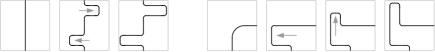
  Figure 11. Details of the moves used in the second step of the evolution of $\Gamma_{1}$.

• it is clear that $\Gamma_{1}$ satisfies (c”), that is, $\ell_{1}(t)$ is increasing in $t$ for $0\leq t\leq 1$, provided that the horizontal and vertical motions employed in the first step are suitably synchronized;

• $\Gamma_{1}$ satisfies the equal-area requirement, Condition  (d’), during the first step because of the symmetry of the evolution;

• $\Gamma_{1}$ satisfies the equal-area requirement, Condition (d’), also during the second step: we remark indeed that every move of the first type in Figure 11 preserves the equal-area condition, while the moves of the second type can be coupled so that to each move that increases the area of one connected component of $\mathscr{Q}\setminus\Gamma_{1}(t)$ (in some square of $\mathcal{T}_{1/5}$) corresponds a move that decreases the area of that component (in another square) by the same amount.

8.12. Construction of $\boldsymbol{\Gamma_{2}(t)}$ for $\boldsymbol{0<t<1}$.

The transition from the curve $\Gamma_{2}(0)$ to the curve $\Gamma_{2}(1)$ is described in Figure 12.

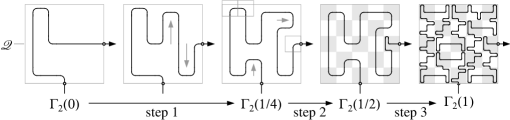
Figure 12. The evolution of $\Gamma_{2}$ from $t=0$ to $t=1$ in three steps.

More precisely, we specify that:

• the small squares drawn in the third picture have side-length $1/5$, and within each of these squares $\Gamma_{2}(1/4)$ agrees with one of the “modified quarter circles” used in §8.10;

• it is clear that  (c”) is satisfied during the entire evolution;

• the equal-area requirement (d’) is satisfied during the first step of this evolution for reasons of symmetry;

• most of $\Gamma_{2}$ is kept fixed by the evolution in the second step, except the part contained in the two squares in the top-left corner of $\mathscr{Q}$, which moves downward, and the part contained in the middle square on the right side, which evolves according to the second move in Figure 11; the equal-area requirement (d’) is satisfied at time $t=1/2$, and is satisfied also for the intermediate times $1/4<t<1/2$, provided that these two moves are suitably synchronized by a change of time for one of the two basic moves;

• in the third step, we modify $\Gamma_{2}(1/2)$ within each square in $\mathcal{T}_{1/5}$ (except the middle square on in the right side of $\mathscr{Q}$) using one of the moves described in Figure 11; note that this step satisfies the equal-area requirement (d’) for the same reasons as in the last step of the evolution of $\Gamma_{1}$.

References

- [1] G. Alberti, S. Bianchini, and G. Crippa. Structure of level sets and Sard-type properties of Lipschitz maps. Ann. Sc. Norm. Super. Pisa Cl. Sci. (5), 12(4):863–902, 2013.
- [2] G. Alberti, S. Bianchini, and G. Crippa. A uniqueness result for the continuity equation in two dimensions. J. Eur. Math. Soc. (JEMS), 16(2):201–234, 2014.
- [3] G. Alberti, G. Crippa, and A. L. Mazzucato. Exponential self-similar mixing and loss of regularity for continuity equations. C. R. Math. Acad. Sci. Paris, 352(11):901–906, 2014.
- [4] G. Alberti, G. Crippa, and A. L. Mazzucato. Loss of regularity for continuity equations with non-Lipschitz velocity. 2018. Preprint. arXiv:1802.02081.
- [5] L. Ambrosio. Transport equation and Cauchy problem for BV vector fields. Invent. Math., 158(2):227–260, 2004.
- [6] L. Ambrosio and G. Crippa. Continuity equations and ODE flows with non-smooth velocity. Proc. Roy. Soc. Edinburgh Sect. A, 144(6):1191–1244, 2014.
- [7] H. Aref. Stirring by chaotic advection. J. Fluid Mech., 143:1–21, 1984.
- [8] H. Bahouri, J.-Y. Chemin, and R. Danchin. Fourier analysis and nonlinear partial differential equations. Grundlehren der Mathematischen Wissenschaften, 343. Springer-Verlag, Berlin-Heidelberg, 2011.
- [9] J. Bedrossian, N. Masmoudi, and V. Vicol. Enhanced dissipation and inviscid damping in the inviscid limit of the Navier-Stokes equations near the two dimensional Couette flow. Arch. Ration. Mech. Anal., 219(3):1087–1159, 2016.
- [10] J. Bergh and J. Löfström. Interpolation spaces. An introduction. Grundlehren der Mathematischen Wissenschaften, 223. Springer-Verlag, Berlin-Heidelberg, 1976.
- [11] S. Bianchini and P. Bonicatto. A uniqueness result for the decomposition of vector fields in . 2017. Preprint SISSA.
- [12] G. Boffetta, A. Celani, M. Cencini, G. Lacorata, and A. Vulpiani. Nonasymptotic properties of transport and mixing. Chaos, 10(1):50–60, 2000.
- [13] F. Bouchut and G. Crippa. Lagrangian flows for vector fields with gradient given by a singular integral. J. Hyperbolic Differ. Equ., 10(2):235–282, 2013.
- [14] D. Bresch and P.-E. Jabin. Global existence of weak solutions for compresssible Navier–Stokes equations: Thermodynamically unstable pressure and anisotropic viscous stress tensor. Ann. of Math., 188:577–684, 2018.
- [15] A. Bressan. A lemma and a conjecture on the cost of rearrangements. Rend. Sem. Mat. Univ. Padova, 110:97–102, 2003.
- [16] E. Brué and Q.-H. Nguyen. Sharp regularity estimates for solutions of the continuity equation drifted by Sobolev vector fields. 2018. Preprint. arXiv:1806.03466.
- [17] F. Colombini, T. Luo, and J. Rauch. Nearly Lipschitzean divergence-free transport propagates neither continuity nor BV regularity. Commun. Math. Sci., 2(2):207–212, 2004.
- [18] P. Constantin, A. Kiselev, L. Ryzhik, and A. Zlatoš. Diffusion and mixing in fluid flow. Ann. of Math. (2), 168(2):643–674, 2008.
- [19] G. Crippa and C. De Lellis. Estimates and regularity results for the DiPerna-Lions flow. J. Reine Angew. Math., 616:15–46, 2008.
- [20] G. Crippa and C. Schulze. Cellular mixing with bounded palenstrophy. Math. Models Methods Appl. Sci., 27(12):2297–2320, 2017.
- [21] N. Depauw. Non unicité des solutions bornées pour un champ de vecteurs BV en dehors d’un hyperplan. C. R. Math. Acad. Sci. Paris, 337(4):249–252, 2003.
- [22] E. Di Nezza, G. Palatucci, and E. Valdinoci. Hitchhiker’s guide to the fractional Sobolev spaces. Bull. Sci. Math., 136(5):521–573, 2012.
- [23] R. J. DiPerna and P.-L. Lions. Ordinary differential equations, transport theory and Sobolev spaces. Invent. Math., 98(3):511–547, 1989.
- [24] D. P. G. Foures, C. P. Caulfield, and P. J. Schmid. Optimal mixing in two-dimensional plane Poiseuille flow at finite Péclet number. J. Fluid Mech., 748:241–277, 2014.
- [25] T. Gotoh and T. Watanabe. Scalar flux in a uniform mean scalar gradient in homogeneous isotropic steady turbulence. Phys. D, 241(3):141–148, 2012.
- [26] E. Gouillart, O. Dauchot, J.-L. Thiffeault, and S. Roux. Open-flow mixing: Experimental evidence for strange eigenmodes. Phys. Fluids, 21(2):023603, 2009.
- [27] L. Grafakos. Modern Fourier analysis. Graduate Texts in Mathematics, 250. Springer-Verlag, New York, third edition, 2014.
- [28] G. Iyer, A. Kiselev, and X. Xu. Lower bounds on the mix norm of passive scalars advected by incompressible enstrophy-constrained flows. Nonlinearity, 27(5):973–985, 2014.
- [29] P.-E. Jabin. Critical non-Sobolev regularity for continuity equations with rough velocity fields. J. Differential Equations, 260(5):4739–4757, 2016.
- [30] M.-C. Jullien. Dispersion of passive tracers in the direct enstrophy cascade: Experimental observations. Phys. Fluids, 15(8):2228–2237, 2003.
- [31] M.-C. Jullien, P. Castiglione, and P. Tabeling. Experimental observation of Batchelor dispersion of passive tracers. Phys. Rev. Lett., 85(17):3636–3639, 2000.
- [32] A. Kiselev and X. Xu. Suppression of chemotactic explosion by mixing. Arch. Ration. Mech. Anal., 222(2):1077–1112, 2016.
- [33] F. Léger. A new approach to bounds on mixing. Math. Models Methods Appl. Sci., 2018. In press.
- [34] Z. Lin, J.-L. Thiffeault, and C. R. Doering. Optimal stirring strategies for passive scalar mixing. J. Fluid Mech., 675:465–476, 2011.
- [35] W. Liu. Mixing enhancement by optimal flow advection. SIAM J. Control Optim., 47(2):624–638, 2008.
- [36] C. Liverani. On contact Anosov flows. Ann. of Math. (2), 159(3):1275–1312, 2004.
- [37] E. Lunasin, Z. Lin, A. Novikov, A. L. Mazzucato, and C. R. Doering. Optimal mixing and optimal stirring for fixed energy, fixed power, or fixed palenstrophy flows. J. Math. Phys., 53(11):115611, 2012.
- [38] G. Mathew, I. Mezić, S. Grivopoulos, U. Vaidya, and L. Petzold. Optimal control of mixing in Stokes fluid flows. J. Fluid Mech., 580:261–281, 2007.
- [39] G. Mathew, I. Mezic, and L. Petzold. A multiscale measure for mixing. Phys. D, 211(1-2):23–46, 2005.
- [40] J. M. Ottino. The kinematics of mixing: stretching, chaos, and transport. Cambridge Texts in Applied Mathematics. Cambridge University Press, Cambridge, 1989.
- [41] D. Rothstein, E. Henry, and J. P. Gollub. Persistent patterns in transient chaotic fluid mixing. Nature, 401(6755):770–772, 1999.
- [42] C. Seis. Maximal mixing by incompressible fluid flows. Nonlinearity, 26(12):3279–3289, 2013.
- [43] M. Taylor. Equivalence of Euclidean and toral Sobolev norms. Private communication, 2016.
- [44] H. Triebel. Theory of function spaces. Monographs in Mathematics, 78. Birkhäuser Verlag, Basel, 1983.
- [45] Y. Yao and A. Zlatoš. Mixing and un-mixing by incompressible flows. J. Eur. Math. Soc. (JEMS), 19(7):1911–1948, 2017.
- [46] C. Zillinger. On geometric and analytic mixing scales: comparability and convergence rates for transport problems. 2018. Preprint. arXiv:1804.11299.