Nonequilibrium Kinetics of One-Dimensional Bose Gases

Abstract

We study cold dilute gases made of bosonic atoms, showing that in the mean-field one-dimensional regime they support stable out-of-equilibrium states. Starting from the 3D Boltzmann-Vlasov equation with contact interaction, we derive an effective 1D Landau-Vlasov equation under the condition of a strong transverse harmonic confinement. We investigate the existence of out-of-equilibrium states, obtaining stability criteria similar to those of classical plasmas.

1 Introduction

Bose [1] and Fermi degeneracy [2] were achieved some years ago in experiments with ultracold alkali-metal atoms, based on laser-cooling and magneto-optical trapping. These experiments have opened the way to the investigation and manipulation of novel states of atomic matter, like the Bose-Einstein condensate [3] and the superfluid Fermi gas in the BCS-BEC crossover [4]. Simple but reliable theoretical tools for the study of these systems in the collisional regime are the hydrodynamic equations [3, 5]. Nevertheless, to correctly reproduce dynamical properties of atomic gases in the mean-field collisionless regime [6, 7], or in the crossover from collisionless to collisional regime [8], one needs the Boltzmann-Vlasov equation [9, 10, 11, 12]. Indeed, the Boltzmann-Vlasov equation is believed to be the correct equation to investigate the kinetics of a generic quantum gas made of out-of-condensate atoms [13]. For dilute and cold atomic gases the mean-field potential of the Boltzmann-Vlasov equation [9, 10, 11] is proportional to the s-wave scattering length of the inter-atomic interaction and to the local density of the gas [6, 13]. In the mean-field collisionless regime, where the interaction time between atoms is much larger than the characteristic period of the analyzed phenomenon, one can safely neglect the collisional integral of the Boltzmann-Vlasov equation getting the Landau-Vlasov equation, also called Hartree-Vlasov equation [9].

The collisionless regime is strongly enhanced for a bosonic gas in a quasi one-dimensional (1D) configuration. A 3D system is said quasi-1D when the single-particle axial energy is much smaller than the energy of the transverse confinement. Quasi-1D systems are nowadays routinely engineered with ultracold atoms in optical potentials, with harmonic transverse confinement energies much larger than the gas temperature or chemical potential [14]. Remarkably, in a strictly 1D system of identical particles no thermalization may possibly occur [15]; such a behavior has been observed with cold bosonic atoms trapped in a 1D optical lattice [16]. Indeed, particles completely exchange their energy in 1D binary elastic collisions, so, if they are indistinguishable, no sensible outcome is produced by such collisions. For 1D bosonic gases the collisionless Vlasov equation can be safely used under the condition $\lambda_{dB}\ll d\ll l_{c}$ [15], where $\lambda_{dB}=(2\pi\hbar)/\sqrt{2\pi mk_{B}T}$ is the de Broglie wavelength with $T$ the absolute temperature, $d=1/\rho$ is the average distance between particles with $\rho$ the 1D local density, and $l_{c}=\hbar/\sqrt{mg\rho}$ is the correlation length with $g\rho$ the 1D mean-field potential and $g$ the 1D effective interaction strength of the inter-atomic potential. It is well know that in a 1D bosonic system Bose-Einstein condensation is forbidden but quasi-condensation is possible [3, 9]; these inequalities ensure that the 1D bosonic gas does not contain a quasi-condensate (the classical description is applicable) and that it does not acquire the fermionic properties characteristic of the Tonks-Girardeau gas [15].

In this paper we consider the consequences of a strong confinement in the transverse plane and, assuming $\lambda_{dB}\ll d\ll l_{c}$, we derive an effective 1D Landau-Vlasov equation from its 3D analog. The resulting 1D equation is similar to the 3D starting one, except for the renormalization of the inter-atomic coupling constant by the square of the characteristic length of the transverse confinement. Stimulated by the recent activity on momentum-space engineering for gaseous Bose-Einstein condensates [17], we then apply methods from plasma physics to prove the existence and stability of out-of-equilibrium states for cold bosonic atoms. Specifically, we analyze small fluctuations around stationary solutions of the 1D Landau-Vlasov equation. For fermions, it is well known that zero-sound oscillations describe the perturbations of the Landau-Vlasov equation around the equilibrium Fermi-Dirac distribution [9]. Following the analysis developed by Penrose [18] and Gardner [19] in plasma physics, our investigation generalizes to out-of-equilibrium 1D bosons the original zero-sound Landau result. We also give the dispersion relation for modes associated to broad classes of nonequilibrium solutions of the Landau-Vlasov equation. Finally, we generalize the Penrose criterion of instability to double-peaked distributions of cold bosonic atoms. Although standard in plasma physics, our results points out that cold one-dimensional bosonic gases offer another experimental playground in which the above phenomenology may be investigated.

2 Landau-Vlasov equation and its dimensional reduction

In the absence of Bose-Einstein condensation, cold and dilute gases made of bosonic alkali-metal atoms of mass $m$ are well described by the Boltzmann-Vlasov equation [9, 10, 11, 12]

$$\left[{\partial\over\partial t}+{{\bf p}\over m}\cdot\nabla_{\mathbf{r}}-\nabla_{\mathbf{r}}\big{(}U_{ext}+U_{mf}\big{)}\cdot\nabla_{\bf p}\right]F=I_{coll}[F]\;,$$ (1)

where $F({\bf r},{\bf p},t)$ is the single-particle phase-space distribution. Here,

$$U_{ext}({\bf r})=V(x)+W({\bf r}_{\bot})$$ (2)

is the external trapping potential, due to a generic potential $V(x)$ in the axial direction $x$ and to a harmonic potential

$$W({\bf r}_{\bot})={m\omega_{\bot}^{2}\over 2}(y^{2}+z^{2})$$ (3)

with frequency $\omega_{\bot}$ in the transverse direction ${\bf r}_{\bot}=(y,z)$;

$$U_{mf}({\bf r},t)=\gamma\ n({\bf r},t)$$ (4)

is the mean-field potential due to the inter-atomic interaction, with

$$\gamma={8\pi\hbar^{2}\over m}a_{s}$$ (5)

the interaction strength and $a_{s}$ the s-wave scattering length of the interaction between dilute bosonic atoms [3, 15]. Nonlinerarities in the left-hand side of Eq. (1) arise from the 3D local density $n({\bf r},t)$, which is obtained from the phase-space distribution $F({\bf r},{\bf p},t)$ as

$$n({\bf r},t)=\int d^{3}{\bf p}\ F({\bf r},{\bf p},t)\;;$$ (6)

a further spatial integration gives the total number $N$ of atoms:

$$N=\int d^{3}{\bf r}\ n({\bf r},t)\;.$$ (7)

The mean-field potential $U_{mf}({\bf r},t)$, which is linear in $a_{s}$, affects the streaming part of the Boltzmann kinetic equation, while the collision integral $I_{coll}[F]$, which is quadratic in the scattering length $a_{s}$, describes dissipative processes [6]. The collisional integral can be treated within a general formulation [20] or, more simply, within the relaxation-time approximation [6, 21, 22]

$$I_{coll}[F]\simeq-{1\over\tau}\left[F({\bf r},{\bf p},t)-F_{eq}({\bf r},{\bf p})\right]\;,$$ (8)

where $\tau$ is the relaxation time related to the average time between collisions, and $F_{eq}({\bf r},{\bf p})$ is the global equilibrium distribution. By definition, in the mean-field collisionless regime the collisional integral can be neglected: in this case, the phenomenon under investigation has a characteristic time much smaller than the relaxation time [9].

We shall work in this collisionless regime and the 3D Boltzmann-Vlasov equation (1) becomes the so-called 3D Landau-Vlasov (or Hartree-Vlasov) equation [23, 24]:

$$\left[{\partial\over\partial t}+{{\bf p}\over m}\cdot\nabla_{\mathbf{r}}-\nabla_{\mathbf{r}}\big{(}V(x)+W({\bf r}_{\bot})+\gamma\ n({\bf r},t)\big{)}\cdot\nabla_{\bf p}\right]F=0\;.$$ (9)

A further simplification is achieved assuming that the atomic sample is under a very strong transverse confinement due to a large frequency $\omega_{\bot}$ of the trapping harmonic potential [3, 14]. Consistently, we suppose that the transverse energy of the confinement is much larger than the average axial kinetic energy of atoms. Namely,

$$\hbar\omega_{\bot}\gg{\langle p^{2}\rangle\over 2m}\;.$$ (10)

In such a way the 3D system is constrained to occupy the transverse ground state, which is described by a Gaussian probability density of spatial width $a_{\bot}=\sqrt{\hbar/(m\omega_{\bot})}$, thus becoming practically one-dimensional (quasi-1D) [7, 25]. We set

$$F({\bf r},{\bf p},t)=f(x,p,t)\ f_{\bot}({\bf r}_{\bot},{\bf p}_{\bot})\;,$$ (11)

where $f(x,p,t)$ is the time-dependent axial distribution function and $f_{\bot}({\bf r}_{\bot},{\bf p}_{\bot})=f_{\bot}(y,z,p_{y},p_{z})$ is the transverse distribution function, defined as

$$f_{\bot}({\bf r}_{\bot},{\bf p}_{\bot})={1\over\pi^{2}\hbar^{2}}\ \exp{\left(-{{p_{\bot}^{2}\over 2m}+W_{\bot}({\bf r}_{\bot})\over{\hbar\omega_{\bot}\over 2}}\right)}\;$$ (12)

and such that

$$n_{\bot}({\bf r}_{\bot})=\int d^{2}{\bf p}_{\bot}f_{\bot}({\bf r}_{\bot},{\bf p}_{\bot})={1\over\pi a_{\bot}^{2}}\exp{\left(-{(y^{2}+z^{2})\over a_{\bot}^{2}}\right)}\;.$$ (13)

Inserting Eq. (11) into Eq. (9) and taking into account Eqs. (12) and (13), after integration over $y$, $p_{y}$, $z$, $p_{z}$ we are left with the 1D Landau-Vlasov equation

$$\left({\partial\over\partial t}+{p\over m}{\partial\over\partial x}-{\partial\over\partial x}\big{(}V(x)+g\rho(x,t)\big{)}{\partial\over\partial p}\right)f=0\;,$$ (14)

where

$$\rho(x,t)=\int dp\ f(x,p,t)$$ (15)

is the axial local density and

$$g={\gamma}\ \int d^{2}{\bf r}_{\bot}\ n_{\bot}({\bf r}_{\bot})^{2}=\frac{\gamma}{2\pi a_{\bot}^{2}}={4\hbar^{2}a_{s}\over m\,a_{\bot}^{2}}$$ (16)

is the renormalized 1D interaction strength. Notice also that $f(x,p,t)$ is normalized to the total number $N$ of atoms, namely

$$N=\int dx\,dp\ f(x,p,t)\;.$$ (17)

In summary, Eq. (14) is fully reliable for a 1D bosonic gas of cold atoms under two conditions:

$${4\pi\hbar^{2}\rho^{2}\over\langle p^{2}\rangle}\ll 1\;,$$ (18)

ensuring that the 1D Bose gas is not in the quasi-condensate regime, and

$${mg\over\hbar^{2}\rho}={4a_{s}\over\rho\,a_{\bot}^{2}}\ll 1\;,$$ (19)

which implies that the 1D Bose gas is not in the Tonks-Girardeau regime [15]. We remind that a more general derivation of the 1D kinetic equation, valid for a Bose gas characterized by both a quasi-condensate and a thermal component [12], is provided in Ref. [26].

A remark about the possibility of fulfilling conditions (10), (18), (19) in experiments like those reported in Refs. [3, 14, 15] is in order. One can consider an axially uniform gas of alkali-metal atoms with linear density $\rho=N/L$. Typical experimental numbers are $N\simeq 10^{2}$, $a_{s}/a_{\bot}\simeq 10^{-4}$, $L/a_{\bot}\simeq 10^{4}$, so that Eq. (19) is satisfied with ${4a_{s}/(\rho\,a_{\bot}^{2})}\simeq 10^{-2}$. With these experimental values, we have $2\pi N^{2}\left({a_{\bot}/L}\right)^{2}\simeq 10^{-2}$. Thus, even conditions (10) and (18), which can be rewritten as

$$2\pi N^{2}\left({a_{\bot}\over L}\right)^{2}\ll{{\langle p^{2}\rangle\over 2m}\over\hbar\omega_{\bot}}\ll 1\;,$$ (20)

are fulfilled with the choice

$$\langle p^{2}\rangle/(2m)\simeq 10^{-1}\hbar\omega_{\bot}\;,$$ (21)

a reasonable request in experimental setups. For the important parameters $N$ and $\frac{a_{s}}{a_{\perp}}$ Eqs. (10), (18), (19) set the ranges $10\leq N\leq 5\cdot 10^{2}$ and $10^{-4}\leq\frac{a_{s}}{a_{\bot}}\leq 5\cdot 10^{-2}$.

3 Stationary states

In this section we further simplify our analysis by dropping the axial confinement, $V(x)=0$. The absence of an external axial potential is clearly a simplification. However, it is possible to experimentally produce 1D configurations of ultracold atoms without axial confinement by using a 1D ring geometry with a large radius [16] or, alternatively, by adopting a straight axial 1D configuration with two high barriers at the edges [27]. Consequently, the 1D Landau-Vlasov equation becomes

$$\left({\partial\over\partial t}+{p\over m}{\partial\over\partial x}-g\int d{\tilde{p}}{\partial f(x,{\tilde{p}},t)\over\partial x}\ {\partial\over\partial p}\right)f(x,p,t)=0\;.$$ (22)

Formally, any stationary and spatially uniform phase-space distribution $f_{0}(p)$ satisfies Eq. (22), but of course the mere existence of a solution does not implies its stability. In general it is not required for $f_{0}(p)$ to coincide with the thermal equilibrium distribution; the subject of our investigations is instead the dynamical stability of experimentally-engineered (out-of-equilibrium) $f_{0}(p)$’s.

Let $f_{0}(p)$ be a general spatially uniform 1D distribution function; we can set

$$f(x,p,t)=f_{0}(p)+\delta f(x,p,t)\;,$$ (23)

where $\delta f$ is considered a small perturbation around the stationary solution. At linear order, $\delta f$ satisfies

$$\left({\partial\over\partial t}+{p\over m}{\partial\over\partial x}\right)\delta f(x,p,t)-g{\partial f_{0}(p)\over\partial p}\int d{\tilde{p}}\;{\partial\,{\delta f}(x,{\tilde{p}},t)\over\partial x}=0\;.$$ (24)

Following Landau’s steps in plasma theory, the stability of $f_{0}$ can be assessed by considering the initial-value problem [28, 29]

$$\frac{\partial\delta f}{\partial t}+\frac{p}{m}\frac{\partial\delta f}{\partial x}-g\int d\tilde{p}\frac{\partial\delta f}{\partial x}(x,\tilde{p},t)\frac{\partial f_{0}}{\partial p}(p)=\delta f_{0}\;\delta(t)\;,$$ (25)

with the prescription $\delta f(x,p,t)=0$ for $t<0$. Indeed, the Dirac $\delta$-function in time brings the system to the perturbed initial state $f=f_{0}+\delta f$, characterized by $\delta f(x,p,0)=\delta f_{0}(x,p)$. The time evolution of the perturbation determines whether $f_{0}$ is stable ($\delta f$ damps away), unstable ($\delta f$ grows up), or marginally stable (the amplitude of $\delta f$ remains constant).

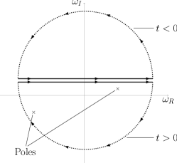
Figure 1: Integration path $\Gamma_{\omega}$ for $t\lessgtr 0$.

This initial-value problem is most easily addressed through a generalized Fourier-transform pair, involving a complex frequency $\omega=\omega_{R}+\mathrm{i}\omega_{I}$:

$$\delta\tilde{f}(k,p,\omega)=\int dx\,dt\;\delta{f}(x,p,t)\,\mathrm{e}^{-\mathrm{i}(kx-\omega t)};\,$$ (26)

$$\delta f(x,p,t)=\int_{\Gamma_{\omega}}dk\,d\omega\;\delta\tilde{f}(k,p,\omega)\,\mathrm{e}^{\mathrm{i}(kx-\omega t)}\;.$$ (27)

In order to satisfy the causality requirement ($\delta f=0$ for $t<0$), the integration path $\Gamma_{\omega}$ in the complex $\omega$-plane can be chosen as a straight line parallel to the real axis, lying above all singularities of $\delta\tilde{f}$. At $\omega_{R}=\pm\infty$, such a path can be closed by the portion of a circular line of infinite radius in the upper (lower) $\omega$-plane for $t<0$ ($t>0$) (see Fig. 1). By virtue of the residues theorem one thus sees that, among all possible modes, those that determine the time evolution of the perturbation are related to the poles of $\delta\tilde{f}$ in the complex $\omega$-plane.

In view of Eq. (25), $\delta\tilde{f}$ satisfies

$$\bigg{(}-\omega+\frac{p}{m}k\bigg{)}\delta\tilde{f}-gk\int d\tilde{p}\;\delta\tilde{f}(k,\tilde{p},\omega)\frac{\partial f_{0}(p)}{\partial p}=\frac{\delta\tilde{f}_{0}}{2\pi i}$$ (28)

or

$$\delta\tilde{f}(k,p,\omega)=\frac{1}{2\pi ik}\frac{\delta\tilde{f}_{0}(k,p)}{\big{(}\frac{p}{m}-\frac{\omega}{k}\big{)}}+\frac{g\frac{\partial f_{0}(p)}{\partial p}}{\big{(}\frac{p}{m}-\frac{\omega}{k}\big{)}}\int d\tilde{p}\;\delta\tilde{f}(k,\tilde{p},\omega)\;.$$ (29)

Integrating over $p$ we get

$$\int dp\;\delta\tilde{f}(k,p,\omega)=-\frac{i}{2\pi k\,\epsilon(k,\omega)}\int dp\;\delta\tilde{f}_{0}\bigg{(}\frac{p}{m}-\frac{\omega}{k}\bigg{)}^{-1}\;,$$ (30)

with

$$\epsilon(k,\omega)=1-g\int dp\,\frac{\partial f_{0}(p)}{\partial p}\bigg{(}\frac{p}{m}-\frac{\omega}{k}\bigg{)}^{-1}\;.$$ (31)

For non-pathological choices of the initial perturbation $\delta f_{0}$, the integral at the r.h.s. of Eq. (30) is well defined by appropriate choices of the integration path (see below). According to Eq. (30), the singular behavior of $\delta\tilde{f}$ is then characterized by the dispersion relation

$$\epsilon(k,\omega)=0\;,$$ (32)

which identifies the poles of $\delta\tilde{f}$.

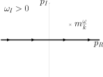
(a)

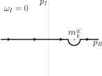
(b)

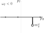
(c)

Figure 2: Integration paths in the complex $p$-plane for the analytical extension of $\epsilon(k,\omega)$.

In analogy with plasma physics, $\epsilon(k,\omega)$ can be viewed as a dielectric function. In many-body physics it is called susceptibility or response function. Since the integration path $\Gamma_{\omega}$ is originally defined as a straight line lying above all singularities, the dielectric function is well defined for sufficiently large positive $\omega_{I}$. In such a case, the integral at the r.h.s. of Eq. (31) lies on the real $p$-axis, below the pole at $m\omega/k$. In order to close the integration path $\Gamma_{\omega}$ in the lower $\omega$-plane, to evaluate the time evolution of the perturbation for $t>0$, we must correspondingly extend analytically $\epsilon$ from the upper to the lower $\omega$-plane. Complex analysis guarantees that the analytical extension is achieved by deforming the integration path on the real $p$-axis in such a way that it encircles the singularity at $m\omega/k$ from below (see Fig. 2). If $\omega_{I}=0$ such a detour contributes for half the residue at the pole; whereas if $\omega_{I}<0$ the contribution amounts to the full residue.

In summary, depending on the sign of $\omega_{I}$ we get three different explicit dispersion relation $\epsilon(k,\omega)=0$ [18, 19]:

$$1 - g\int_{-\infty}^{+\infty}dp\;{{f_{0}^{\prime}}(p)\over p/m-\omega/k}=0\quad\mbox{for}\;\omega_{I}>0\;,$$ (33)

$$1 - g\;\mathcal{P}\int_{-\infty}^{+\infty}dp\;{{f_{0}^{\prime}}(p)\over p/m-\omega/k}-\pi i\,g\,f_{0}^{\prime}(m\omega/k)=0\quad\mbox{for}\;\omega_{I}=0\;,$$ (34)

$$1 - g\int_{-\infty}^{+\infty}dp\;{{f_{0}^{\prime}}(p)\over p/m-\omega/k}-2\pi i\,g\,f_{0}^{\prime}(m\omega/k)=0\quad\mbox{for}\;\omega_{I}<0\;,$$ (35)

where $f_{0}^{\prime}(p)\equiv\partial f_{0}(p)/\partial p$, and the symbol $\mathcal{P}$ indicates the principal part of the integral. A solution of the dispersion relation with $\omega_{I}>0$ ($\omega_{I}<0$) corresponds to an exponentially growing (damping) mode. A solution with $\omega_{I}=0$ defines a mode of constant amplitude. As a consequence, the stability of $f_{0}$ is determined by the sign of the imaginary part of the solution of the dispersion relation with the largest $\omega_{I}$.

We remark that these relations are similar to the ones derived for plasmas from the Vlasov-Poisson equation [23, 24]: in that case an additional factor $k^{-1}$ appears in the integrand. In our case, the equation $\epsilon(k,\omega)=0$ shows instead that the dispersion relation between $\omega$ and $k$ is linear and gives implicitly the (complex) phase velocity of the mode,

$$c=\frac{\omega}{k},$$ (36)

as a function of the stationary solution $f_{0}(p)$ and of the parameters $m$ and $g$. It is also worth to point out that if one aims at discussing cases of singular distributions $f_{0}$ containing Dirac-deltas or step functions as in some of the below examples, results can be straightforwardly obtained without employing complex analysis.

3.1 Zero-sound for 1D bosons

As a simple application, let us consider the stationary Fermi-Dirac-like distribution

$$f_{0}(p)=\Theta\left({p_{F}^{2}\over 2m}-{p^{2}\over 2m}\right)\;,$$ (37)

where $\Theta(x)$ is the step function and $p_{F}=\pi\hbar N/L$ is the 1D Fermi-like linear momentum fixed by the normalization (17), with $L$ the length of the axial domain. Under the condition $p_{F}\neq mc$ assuring $f_{0}^{\prime}(mc)=0$, it is straightforward to extract from Eqs. (33), (34), (35) the same result for the phase velocity of the perturbations:

$$c=\pm v_{F}\,\sqrt{1+{2g\over v_{F}}}\;,$$ (38)

where $v_{F}=p_{F}/m$ is the Fermi-like velocity. This formula gives nothing else than the familiar zero-sound velocity of a 1D Fermi gas [9, 10]. Hence, zero-sound measurements can also be performed for 1D bosons in the mean-field collisionless regime by tuning, for example, a stationary Fermi-like distribution of their momenta (37). The two signs ($\pm$) simply mean that the perturbation is characterized by two waves which propagate along the $x$ axis in opposite directions. Equation (38) furthermore tells that such bosonic Fermi-Dirac-like distribution is stable only for $g\geq-v_{F}/2$. We have thus shown that engineering the initial distribution of atomic bosons one gets the typical collisionless dynamics of a Fermi gas around its equilibrium configuration.

3.2 Stability of single-peak distributions and Landau damping

For single-peak distributions $f_{0}(p)$ one can state the following theorem, closely related to the analogous one developed by Penrose [18] and Gardner [19] for the Poisson-Vlasov equations of plasma physics [28, 29].

Theorem. If the spatially uniform initial condition $f_{0}(p)$ has a single maximum and $g>0$, then $f_{0}(p)$ is linearly stable.

Proof.

Let us assume that the contrary is true, namely $c=\omega/k=c_{R}+\mathrm{i}c_{I}$ with $c_{I}>0$. We can rewrite Eq. (33) as

$$1-g\int_{-\infty}^{+\infty}dp\ {(p/m-c_{R}+ic_{I})f_{0}^{\prime}(p)\over(p/m-c_{R})^{2}+c_{I}^{2}}=0\;.$$ (39)

This complex equation can be splitted into two real equations:

$$D_{R}(c_{R},c_{I})\equiv 1-g\int dp\ {(p/m-c_{R})f_{0}^{\prime}(p)\over(p/m-c_{R})^{2}+c_{I}^{2}}=0\;,$$ (40)

$$D_{I}(c_{R},c_{I})\equiv-g\int dp\ {c_{I}\;f_{0}^{\prime}(p)\over(p/m-c_{R})^{2}+c_{I}^{2}}=0\;.$$ (41)

Since $D_{R}(c_{R},c_{I})=0$ and $D_{I}(c_{R},c_{I})=0$, one has also

$$D_{R}(c_{R},c_{I})+{p_{0}/m-c_{R}\over c_{I}}D_{I}(c_{R},c_{I})=0\;,$$ (42)

where we choose $p_{0}$ as the single maximum of the $f_{0}$, satisfying in particular $f_{0}^{\prime}(p_{0})=0$. Equation (42) casts into

$$1+g\int dp\ {(p_{0}/m-p/m)f_{0}^{\prime}(p)\over(p/m-c_{R})^{2}+c_{I}^{2}}=0\;.$$ (43)

In view of the single maximum at $p=p_{0}$,

$$(p_{0}/m-p/m)f_{0}^{\prime}(p)\geq 0\quad\forall p\in(-\infty,+\infty)\;.$$ (44)

This means that the integrand in Eq. (43) is non-negative for all values of $p$. Consequently, for $g>0$ Eq. (43) cannot be satisfied. This proves that our original assumption $c_{I}>0$ ($\omega_{I}>0)$ cannot be correct and that $f_{0}$ is at least marginally stable. ∎

Another situation typical of plasma physics which can be generalized to cold bosonic gases is that of weakly damped waves (or weakly unstable modes), i.e cases with $|\omega_{I}|\ll\omega_{R}$ [28]. ¿From a physical point of view, this amounts to situations in which the amplitude of the perturbations varies little in a time period. Because of the assumption $|\omega_{I}|\ll|\omega_{R}|$, a Taylor expansion of the dielectric function around the real value $\omega_{R}$ leads to

$$\epsilon(k,\omega) = \epsilon(k,\omega_{R}+i\omega_{I})$$

$$\simeq \epsilon(k,\omega_{R})+i\omega_{I}\frac{\partial\epsilon}{\partial\omega_{R}}(k,\omega_{R})\;$$

$$= \epsilon_{R}(k,\omega_{R})+i\epsilon_{I}(k,\omega_{R})+\omega_{I}\bigg{[}i\frac{\partial\epsilon_{R}}{\partial\omega_{R}}(k,\omega_{R})-\frac{\partial\epsilon_{I}}{\partial\omega_{R}}(k,\omega_{R})\bigg{]}.$$

Since $\omega_{I}$ is small, we may still make use of the dispersion relation in the form of Eq. (34), namely

$$\epsilon(k,\omega)=1-g\mathcal{P}\int dp\;\frac{\partial f_{0}(p)}{\partial p}\bigg{(}\frac{p}{m}-\frac{\omega}{k}\bigg{)}^{-1}-i\pi g\frac{\partial f_{0}}{\partial p}\bigg{|}_{p=\frac{m\omega}{k}}\;.$$

Comparing Eq. (34) and Eq. (3.2) we get

$$\epsilon(k,\omega) \simeq 1-g\mathcal{P}\int dp\;\frac{\partial f_{0}}{\partial p}(p)\bigg{(}\frac{p}{m}-\frac{\omega_{R}}{k}\bigg{)}^{-1}-i\pi g\frac{\partial f_{0}}{\partial p}(p)\bigg{|}_{p=\frac{m\omega_{R}}{k}}\;+$$ (46)

$$+\;i\omega_{I}\frac{\partial}{\partial\omega_{R}}\bigg{[}-g\mathcal{P}\int dp\;\frac{\partial f_{0}}{\partial p}(p)\bigg{(}\frac{p}{m}-\frac{\omega_{R}}{k}\bigg{)}^{-1}\bigg{]}+$$

$$+\omega_{I}\frac{\partial}{\partial\omega_{R}}\bigg{[}\pi g\frac{\partial f_{0}}{\partial p}(p)\bigg{|}_{p=\frac{m\omega_{R}}{k}}\bigg{]}\;.$$

To lowest order in $\omega_{I}/\omega_{R}$, we can neglect the last term of the sum in the real part of the dielectric function. The dispersion relation $\epsilon(k,\omega)=0$ gives then two separate equations: for the real part we have

$$1-g\mathcal{P}\int dp\,\frac{\partial f_{0}}{\partial p}(p)\bigg{(}\frac{p}{m}-\frac{\omega_{R}}{k}\bigg{)}^{-1}=0\;;$$ (47)

and for the imaginary one

$$\omega_{I}=-\frac{\pi\frac{\partial f_{0}}{\partial p}\big{(}\frac{m\omega_{R}}{k}\big{)}}{\frac{\partial}{\partial\omega_{R}}\bigg{[}\mathcal{P}\int dp\,\frac{\partial f_{0}}{\partial p}(p)\big{(}\frac{p}{m}-\frac{\omega}{k}\big{)}^{-1}\bigg{]}\bigg{|}_{\omega_{I}=0}}\;.$$ (48)

A simple exemplification of the above theorem and an explicit calculation of the damping rate may be given in terms of the stationary Maxwell-Boltzmann distribution

$$f_{0}(p)=\rho\ {1\over\sqrt{\pi}\overline{p}}e^{-p^{2}/\overline{p}^{2}}\;,$$ (49)

where $\rho=N/L$ is fixed by Eq. (17), with $L$ the length of the axial domain and $\overline{p}$ the characteristic width of the distribution. Under the condition $\overline{p}\ll\sqrt{mg\rho}$ it is not difficult to obtain, by Eq.(47), the real part of the velocity $c_{R}=\omega_{R}/k$ as

$$c_{R}=\pm\sqrt{{g\rho\over m}\left(1+{3\over 2}{\overline{p}^{2}\over mg\rho}\right)}\;,$$ (50)

while, in view of Eq.(48), the imaginary part $c_{I}=\omega_{I}/k$ reads

$$c_{I}=-\sqrt{\pi}\,e^{-3/2}\,{mg^{2}\rho^{2}\over\overline{p}^{3}}\,e^{-mg\rho/\overline{p}^{2}}\;.$$ (51)

This is a meaningful result: the negative sign of $c_{I}$ corresponds to Landau damping, the typical non-collisional phenomenon of wave-particle interaction; in the present case the wave is not an electrostatic [24], but a matter one.

In the limit of vanishing $\overline{p}$, the distribution (49) becomes a Dirac delta function

$$f_{0}(p)=\rho\ \delta\left(p\right)\;,$$ (52)

while the velocity becomes real and given by

$$c=\pm\sqrt{g\rho\over m}\;.$$ (53)

Namely, the zero-sound velocity associated to a strongly localized peak.

3.3 Two-stream instability

We eventually address another interesting situation in which a spatially uniform distribution may not be stable, namely a case with a double-peak $f_{0}(p)$. Arguably, in the simplest case of this kind $f_{0}(p)$ is a linear combination of two Dirac delta,

$$f_{0}(p)=\frac{\rho}{2}\left[\delta(p-p_{0})+\delta(p+p_{0})\right]\;,$$ (54)

representing two streams of particles propagating with the same velocity in opposite directions. By considering the dispersion relation, Eq. (32), for such distribution with $c=\omega/k\neq p_{0}/m$, we obtain

$$c^{2}_{\pm}=\frac{1}{m^{2}}\left(p_{0}^{2}+\frac{1}{2}gm\rho\pm\frac{1}{2}\sqrt{8mg\rho p_{0}^{2}+m^{2}g^{2}\rho^{2}}\right)\;.$$ (55)

Each choice of the $\pm$ sign gives two roots for $c$. If $c^{2}>0$ the two roots are real and, since $k\in\mathbb{R}$, this gives $\omega=\omega_{R}=\pm k\sqrt{c^{2}}$. This is for instance the case of the solution $c^{2}_{+}=\frac{1}{m^{2}}\left(p_{0}^{2}+\frac{1}{2}mg\rho+\frac{1}{2}\sqrt{8mg\rho p_{0}^{2}+m^{2}g^{2}\rho^{2}}\right)$ (with $g>0$). Such a solution describes a circumstance in which $f_{0}$ is marginally stable, the perturbations maintaining constant amplitude and propagating at a velocity

$$c=\pm\sqrt{\frac{1}{m^{2}}\left(p_{0}^{2}+\frac{1}{2}mg\rho+\frac{1}{2}\sqrt{8mg\rho p_{0}^{2}+m^{2}g^{2}\rho^{2}}\right)}\;.$$ (56)

A perhaps more intriguing phenomenology is related to the solution $c^{2}_{-}$, which may turn negative for some values of the parameters. With $c^{2}_{-}<0$ the two roots for $c=\omega/k$ are purely imaginary, equal in magnitude, and opposite in sign. For each given $k$, the positive imaginary root thus characterizes a perturbation exponentially growing in time at a rate $|c_{-}|$. The instability condition $c^{2}_{-}<0$ corresponds to the interval

$$-\sqrt{mg\rho}<p_{0}<\sqrt{mg\rho}\;.$$ (57)

Under these premises, the maximum growth rate $|c_{ins}^{max}|$ is found by maximizing

$$c^{2}_{-}(p_{0})=\frac{1}{m^{2}}\left(p_{0}^{2}+\frac{1}{2}mg\rho-\frac{1}{2}\sqrt{8mg\rho p_{0}^{2}+m^{2}g^{2}\rho^{2}}\right)\;,$$ (58)

and is achieved for $p_{0}=\frac{1}{4}\sqrt{6mg\rho}$ with

$$|c_{ins}^{max}|=\sqrt{\frac{g\rho}{8m}}\;.$$ (59)

More general two-stream instability conditions are given by the following theorem, generalizing the Penrose criterion of plasma physics [18, 28, 29] to cold bosonic gases.

Theorem. If the spatially uniform initial condition $f_{0}(p)$ has two local maxima, a local minumum at $p=p_{min}$, and $g>0$, then $f_{0}(p)$ is unstable under the condition

$$\mathcal{P}\int_{-\infty}^{+\infty}dp\frac{f_{0}(p)-f_{0}(p_{min})}{(p-p_{min})^{2}}>\frac{1}{g\ m}\;.$$ (60)

Proof.

The instability of $f_{0}$ corresponds to the existence of zeros of $\epsilon(k,\omega)$ with a positive imaginary part. If $\epsilon(k,\omega)$ has no poles in the upper $\omega$-plane, the number of such zeros can be computed through the integral

$$\frac{1}{2\pi i}\int_{\Gamma_{\omega}}d\omega\;\frac{1}{\epsilon(k,\omega)}\frac{\partial\epsilon}{\partial\omega}(k,\omega)\;,$$ (61)

where the contour $\Gamma_{\omega}$ runs along the real $\omega$-axis and is then closed counterclockwise by a semicircle of infinite radius in the upper half-plane. The contour $\Gamma_{\omega}$ in the $\omega$-plane maps to a contour $\Gamma_{\epsilon}$ in the $\epsilon$-plane obtained by evaluating $\epsilon(k,\omega)$ at every point of $\Gamma_{\omega}$. The distribution $f_{0}$ is unstable if and only if $\Gamma_{\epsilon}$ encloses the origin. In the present case of two-peak $f_{0}$ this is possible only if the real part of $\epsilon$ evaluated in correspondence of $\omega=\omega_{min}\equiv k\,p_{min}/m$ is negative. An integration by part then leads to the fact that a necessary and sufficient condition for the instability of $f_{0}$ is given by Eq. (60). ∎

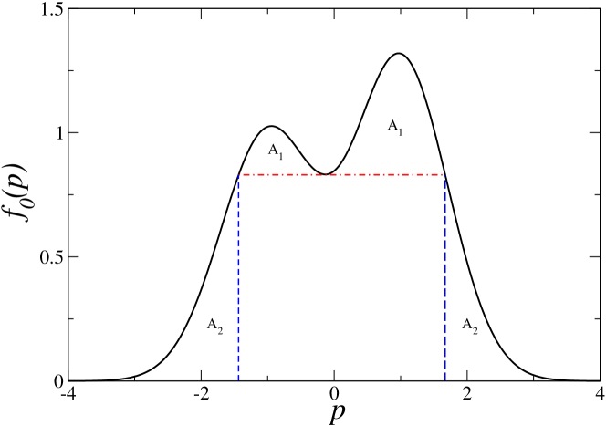
Figure 3: Initial distribution $f_{0}(p)$ with two peaks. Here the local minimum is at $p_{min}=0$. The configuration is unstable if $A_{1}/A_{2}>1/(gm)$, where $A_{1}$ is the area between the portion of $f_{0}(p)$ containing the two maxima and the horizontal dot-dashed line, and $A_{2}$ is the area of the “external” regions delimited by the rest of $f_{0}(p)$, the two vertical dashed lines, and the horizontal axis.

The instability criterion in Eq. (60) has an interesting graphical visualization [28]. Consider the plot $f_{0}(p)$ of Fig. 3 and an horizontal line passing through $f_{0}(p_{min})$. Further consider the vertical segments between the $p$-axis and the intersection points of the horizontal line with $f_{0}(p)$. These vertical lines identify two “external” regions. The left one is delimited by $f(p)$, the portion of $p$-axis including $p=-\infty$, and the left vertical line. Analogously, the right one is delimited by $f(p)$, the portion of $p$-axis including $p=+\infty$, and the right vertical line. The criterion in Eq. (60) means that the area between $f(p)$ and the horizontal line must outweight of at least a factor $1/gm$ the area of the “external” regions. In other words, the dip at the minimum of $f_{0}$ must be sufficiently deep.

At latter, it is pertinent to observe that distributions with two distinct momentum components are now frequently realized with ultracold atoms by means of two-photon Raman and Bragg transitions [31]. Indeed, by adjusting the angle and the frequency difference of the two laser beams driving the transition, each of the two peaks of the imparted momentum can be calibrated within the range $[-1,1]\times 2\hbar k_{L}$, where $\pm\hbar k_{L}$ are the momenta of the laser photons.

4 Axial confinement

Neglecting the axial potential is an assumption that may hinder important dynamical effects (see, e.g., Ref. [32] for a discussion within the context of plasmas). Since most of the experiments are carried out in the presence of an external potential $V(x)$, it is indeed interesting to study numerically the stability of nonequilibrium distributions for given profiles of $V(x)$.

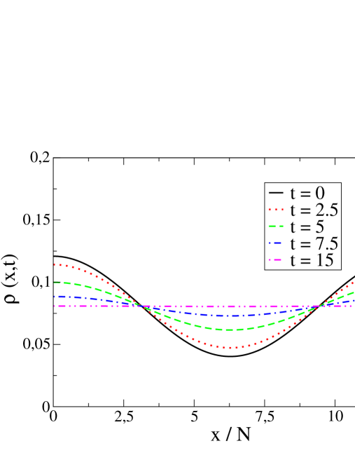
Figure 4: Vlasov time-evolution of the 1D bosonic density profile $\rho(x,t)$. In the simulation units the initial condition is given by Eqs. (49), (62), with $\rho=0.084$, $N=100$, $\overline{p}=0.71$, $\alpha=0.2$, $k=0.5$, $L=12.6\cdot 10^{2}$, and $p_{max}=3$. The interaction strength is fixed at $g=0.1$. The phase space $(x,p)$ has been discretized by a 2D grid of lattice spacing $\Delta x=0.036$ and $\Delta p=0.012$, whereas for the integration time we have chosen $\Delta t=0.005$. Curves correspond to increasing values of time $t$. As time passes by, the initial perturbation is damped out and a stable uniform spatial density is reached.

To integrate numerically Eq. (22) we adopt a semi-Lagrangian scheme with cubic spline interpolation method [30], adapted to the 1D Landau-Vlasov equation for cold bosonic atoms. In order to check the validity of the numerical implementation as well as to compare the relevant time scales of the problem we first analyze the occurrence and time behavior of Landau damping in absence of an axial confinement ($V(x)=0$). In particular we consider the time evolution of the initially perturbed stationary state $f_{0}$:

$$f(x,p,0)=f_{0}(p)[1+\alpha\cos(kx)],\quad x\in[0,L],\;p\in[-p_{max},p_{max}].$$ (62)

where $f_{0}$ is given by Eq. (49).

In order to compare the simulation results with experiments we apply the following procedure. Let us call, respectively, $\mathrm{u_{L}}$, $\mathrm{u_{T}}$, $\mathrm{u_{M}}$ the length, time, and mass units employed in our simulations. The relation between these units and the physical ones can be obtained by equating the values of $\rho(x,t)$, $g$, $\overline{p}$ of the simulations with their typical experimental counterparts, and solving in $\mathrm{u_{L}}$, $\mathrm{u_{T}}$, $\mathrm{u_{M}}$ the resulting system of equations. If we consider reasonable experimental numbers as $N\simeq 100$, $a_{\perp}\simeq 10^{4}a_{s}$ with $a_{s}\simeq 10^{-10}$ m, we get $\rho(x,t)\simeq 10^{4}$ m^-1. Furthermore, taking a Li atom of mass $m\simeq 9\cdot 10^{-27}\;{\rm kg}$, we have $g\simeq 5\cdot 10^{-41}\;{\rm kg\;m^{3}\;s^{-2}}$. Finally, adopting Eq. (21), $\overline{p}\simeq 4\cdot 10^{-29}\;{\rm kg\;m\;s^{-1}}$. Correspondingly, we thus find $1\;\mathrm{u_{L}}=8.4\cdot 10^{-6}\;{\rm m}$, $1\;\mathrm{u_{T}}=0.2\;{\rm s}$, $1\;\mathrm{u_{M}}=3\cdot 10^{-27}\;{\rm kg}$.

In Figure 4 we show the density profile $\rho(x,t)$ taken at different time steps. As expected by the considerations given in section 3, the initial perturbation damps down to a spatially uniform density profile with a damping time $\tau_{D}\simeq 10\;\mathrm{u_{T}}=2\;\mathrm{s}$. Nowadays, experimental duration time of the order of seconds are indeed at reach.

Although collisions are effectless in strictly 1D configurations, they still provide a thermalization mechanism to quasi-1D systems. It is then interesting to compare the typical collision time with the the Landau damping time $\tau_{D}$. The collision time $\tau_{c}$ can be estimated as [21]

$$\tau_{c}\simeq\frac{1}{n\sigma\overline{v}},$$ (63)

where $\overline{v}=\overline{p}/m$ is the characteristic velocity of the particles, and $\sigma=8\pi a_{s}^{2}$ is the cross-section. For our quasi-1D setup we may take $n=\rho/(2\pi a_{\bot}^{2})$ with $\rho=N/L$, and $\tau_{c}$ then reads $\tau_{c}=1/(4\rho(a_{s}/a_{\bot})^{2}\overline{p}/m)$. Adopting this time natural units with $\hbar=m=1$, from Eq. (16) one finds $a_{s}^{2}=g^{2}a_{\bot}^{4}/16$ and consequently $\tau_{c}=4/(\rho g^{2}L^{2}\overline{p}(a_{\bot}/L)^{2})$. By using the values in the caption of Fig. 4 we then obtain $\tau_{c}\simeq 7\cdot 10^{3}\,(L/a_{\bot})^{2}$. We notice that the collisional time is proportional to the $L/a_{\perp}$; in order to obtain realistic quasi-1D configurations, this ratio has to be engineered such that $L/a_{\perp}\simeq 10$ or more. If we impose that this ratio is $10$, then the collision time is $\tau\simeq 10^{5}$, four orders of magnitude larger than the damping time $\tau_{D}$.

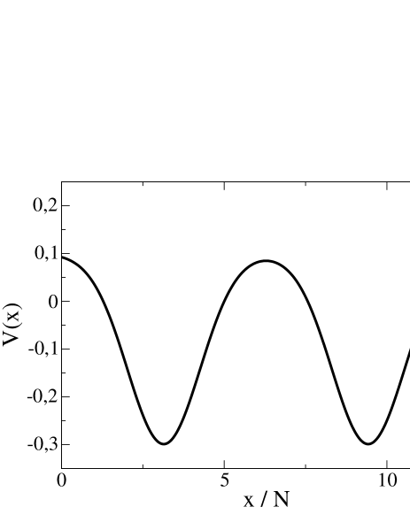
Figure 5: The axial potential defined in Eq. (64) for $s=1.58$, $x_{0}=L/4$, $x_{1}=3L/4$, $N=100$, and system size $L=12.6\cdot 10^{2}$.

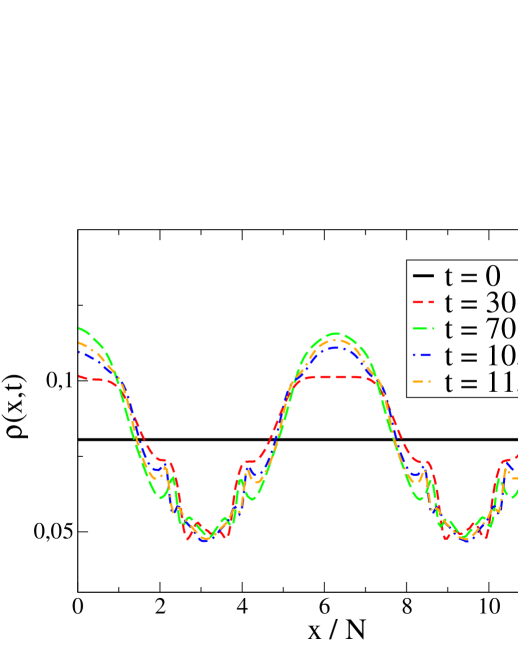
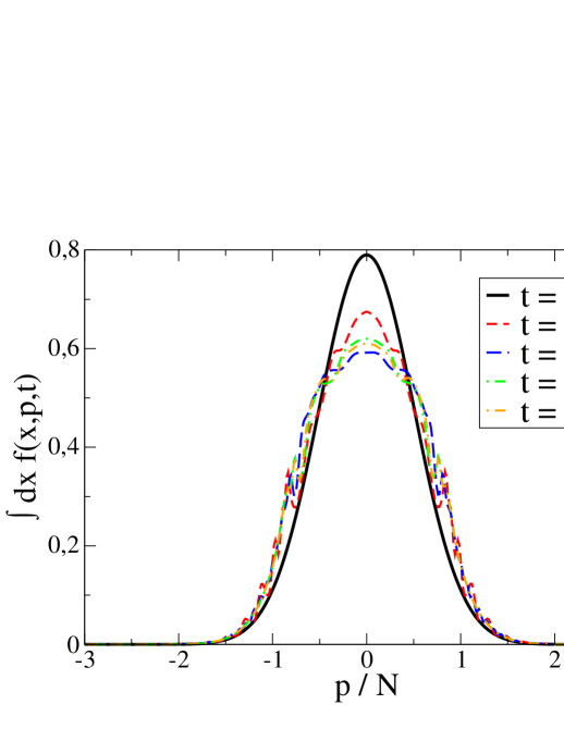
Figure 6: Vlasov time-evolution in the presence of the external potential $V(x)$ in Fig. 5. In the simulation units, the initial 1D distribution (see solid and thicker curves in both panels) is set to be uniform along $x$ with density $\rho=0.084$ (top panel) and Gaussian in the momenta space as in Eq. (49) with $\overline{p}=0.71$ and $p_{max}=3$ (bottom panel). As in Figure 4, $N=100$, $g=0.1$, $\Delta x=0.036$, $\Delta p=0.012$ and $\Delta t=0.005$. In both panels the dashed curves refer to the density $\rho(x,t)$ and the reduced probability distribution $\int f(x,p,t)dx$ profiles taken at different times. Note that, as $t$ increases, the curves tend to stabilize around a non-Gaussian shape.

We now consider the system in the presence of a symmetric external axial potential of double-well shape:

$$V(x)=-\frac{1}{\sqrt{2\pi}}\left[e^{-\frac{(x-x_{0})^{2}}{s^{2}}}+e^{-\frac{(x-x_{1})^{2}}{s^{2}}}\right]$$ (64)

(see Fig. 5). The effect of this potential on an initially uniform spatial profile and momenta distribution as in Eq. (49) is reported in Fig. 6: it is readily seen that Landau damping provide a relaxation mechanism alternative to collisions which drives the system to a stationary state reproducing the double-well shape of the potential. This implies that the switch on of a potential acts as a perturbation which interacts with the gas atoms in a sort of wave-particle energy exchange, similarly to the standard interpretation of Landau damping.

5 Conclusions

Within a mean-field collisionless regime, we have shown that stable out-of-equilibrium states can be produced with 1D Bose gases made of cold alkali-metal atoms. This prediction is based on the analysis of the effective 1D Landau-Vlasov equation derived from the 3D Boltzmann equation under the condition of a strong transverse confinement. By investigating the linearized 1D Landau-Vlasov equation, we have obtained theorems addressing the stability of such out-of-equilibrium solutions. Emphasizing analogies with plasma physics, we have been able to point out the existence of a variegate phenomenology also applicable to experimental design for cold 1D bosonic gases. Results include zero-sound transmission for bosonic species, Landau damping, and two-stream instability. On longer time scales controlled by the length-to-width ratio of the quasi-1D configuration, residual correlations and many-atom collisional effects are expected to erase such phenomena as a side effect of the approach to equilibrium. Finally, as a simple but meaningful example, we have shown that switching on suddenly an external double-well potential $V(x)$ the atomic cloud goes towards a new out-of-equilibrium stationary configuration. Similar configurations, obtained with different external potentials $V(x)$ and initial conditions, are presently under investigation.

Acknowledgments. The authors thank David Guery-Odelin, Francesco Minardi, Roberto Onofrio, Flavio Toigo for useful suggestions and acknowledge Ministero Istruzione Universita Ricerca (PRIN project 2010LLKJBX) for partial support.

References

References

- [1] M.H. Anderson, J.R. Ensher, M.R. Matthews, C.E. Wieman, and E.A. Cornell, Science 269, 198 (1995).
- [2] B. DeMarco and D. Jin, Science 285, 1703 (1999).
- [3] F. Dalfovo, S. Giorgini, L. P. Pitaevskii, and S. Stringari, Rev. Mod. Phys. 71, 463 (1999).
- [4] S. Giorgini, L. P. Pitaevskii, and S. Stringari, Rev. Mod. Phys. 80, 1215 (2008).
- [5] S.K. Adhikari and L. Salasnich, New J. Phys. 11, 023011 (2009).
- [6] P. Pedri, D. Guery-Odelin, and S. Stringari, Phys. Rev. A 68, 043608 (2003).
- [7] G. Mazzarella, L. Salasnich, and F. Toigo, Phys. Rev. A 79, 023615 (2009).
- [8] Z. Akdeniz, P. Vignolo, and M.P. Tosi, Phys. Lett. A 311, 246 (2003); P. Capuzzi, P. Vignolo, F. Federici, and M.P. Tosi, J. Phys. B: At. Mol. Opt. Phys. 39, S25 (2006).
- [9] L. Landau and L. Lifshitz, Course in Theoretical Physics, Vol. 9, Statistical Physics - Part 2 (Pergamon, New York, 1959).
- [10] D. Pines and P. Noziers, The Theory of Quantum Liquids, Vol I, Normal Fermi Liquids (W.A. Benjamin, New York, 1966).
- [11] L.P. Kadanoff and G. Baym, Quantum Statistical Mechanics (Benjamin, New York, 1962).
- [12] E. Zaremba, T. Nikuni, and A. Griffin, J. Low Temp. Phys. 116, 277 (1999).
- [13] A. Griffin, T. Nikuni, and E. Zaremba, Bose-Condended Gases at Finite Temperature (Cambridge Univ. Press, Cambridge, 2009).
- [14] T. Langen, Non-equilibrium Dynamics of One-Dimensional Bose Gases (Springer, Cham, 2015).
- [15] D. Guery-Odelin, Phys. Rev. A 66, 033613 (2002).
- [16] T. Kinoshita, T.R. Wenger, and D.S. Weiss, Nature 440, 900 (2006).
- [17] L. Deng, E.W. Hagley, J. Denschlag, J.E. Simsarin, M. Edwards, C.W. Clark, K. Helmerson, S.L. Rolston, and W.D. Phillips, Phys. Rev. Lett 83, 5407 (1999); M. Edwards, B. Benton, J. Heward, C.W. Clark, Phys. Rev. A 82, 063613 (2010); W. Xiong, X. Yue, Z. Wong, X. Zhou, and X. Chen, Phys. Rev. A 84, 043616 (2011).
- [18] O. Penrose, Phys. Fluids 3, 258 (1960).
- [19] C.S. Gardner, Phys. Fluids 6, 839 (1963).
- [20] S. Gupta, Z. Hadzibabic, J.R. Anglin, and W. Ketterle, Phys. Rev. Lett. 92, 100401 (2004).
- [21] K. Huang, Statistical Mechanics (Wiley, New York, 1984).
- [22] A. Antoniazzi, F. Califano, D. Fanelli, and S. Ruffo, Phys. Rev. Lett. 98, 150602 (2007); A. Antoniazzi, D. Fanelli, S. Ruffo, Y. Yamaguchi, Phys. Rev. Lett. 99, 040601 (2007).
- [23] A. Vlasov, J. Phys. U.S.S.R. 9, 25 (1945).
- [24] L. Landau, J. Phys. U.S.S.R. 10, 25 (1946).
- [25] L. Salasnich and F. Toigo, J. Low Temp. Phys. 150, 643 (2008).
- [26] E. Arahata and T. Nikuni, J. Low Temp. Phys. 171, 369 (2013).
- [27] K.E. Strecker, G.B. Partridge1, A.G. Truscott, and R.G. Hulet, Nature 417, 150 (2002).
- [28] P.A. Sturrock, Plasma Physics: An Introduction to the Theory of Astrophysical, Geophysical and Laboratory Plasmas (Cambridge University Press, 1994).
- [29] D.R. Nicholson, Introduction to Plasma Theory (Wiley, New York, 1983).
- [30] C.Z Cheng and G. Knorr, J. Comp. Phys. 22, 350 (1976).
- [31] M. Weidemüller and C Zimmermann (Eds.), Interactions in Ultracold Gases: From Atoms to Molecules (Wiley, Weinheim, 2003).
- [32] A. Jackson, M. Raether, Phys. Fluids 9, 1257 (1966).