The tempered discrete Linnik distribution

LUCIO BARABESI
Department of Economics & Statistics, University of Siena, Italy  CAROLINA BECATTI
Department of Economics & Statistics, University of Siena, Italy  MARZIA MARCHESELLI
Department of Economics & Statistics, University of Siena, Italy

ABSTRACT. A tempered version of the discrete Linnik distribution is introduced in order to obtain integer-valued distribution families connected to stable laws. The proposal constitutes a generalization of the well-known Poisson-Tweedie law, which is actually a tempered discrete stable law. The features of the new tempered discrete Linnik distribution are explored by providing a series of identities in law - which describe its genesis in terms of mixture and compound Poisson law, as well as in terms of mixture discrete stable law. A manageable expression of the corresponding probability function is also provided and several special cases are analysed.

Key words: Lévy-Khintchine representation; Positive Stable distribution; Discrete Stable distribution; Mixture Poisson distribution; Compound Poisson distribution.

MSC 2010 Primary 62E10, secondary 62E15.

1. Introduction In recent years, heavy-tailed models - in primis, stable distributions - have been used in a variety of fields, such as statistical physics, mathematical finance and financial econometrics (see e.g. Rachev et al., 2011, and references therein). However, these models may be partially appropriate to provide a good fit to data, since their tails are too “fat” to describe empirical distributions, as remarked by Klebanov and& Slámová (2015). In order to overcome this drawback, the so-called “tempered” versions of heavy-tailed distributions have been successfully introduced (see e.g. Rosínski, 2007). Indeed, tempering allows for models that are similar to original distributions in some central region, even if possess lighter - i.e. tempered - tails. Klebanov & Slámová (2015) have suitably discussed these issues and have suggested various tempering techniques - emphasizing that tempering is not necessarily unambiguous.

In the framework of integer-valued laws, the Poisson-Tweedie is a well-known tempered distribution introduced independently by Gerber (1991) and Hougaard et al. (1997). This law is de facto the tempered counterpart of the Discrete Stable law originally suggested by Steutel & van Harn (1979). The Poisson-Tweedie distribution encompasses classical families (such as the Poisson), as well as large families (such as the Generalized Poisson Inverse Gaussian and the Poisson-Pascal). Hence, this law may be very useful for modelling data arising in a plethora of frameworks - for example, clinical experiments (Hougaard, Lee & Whitmore, 1997), environmental studies (El-Shaarawi, Zhu & Joe, 2011) and scientometric analysis (Baccini, Barabesi & Stracqualursi, 2016).

Christoph & Schreiber (1998) emphasize that the Discrete Stable distribution may be seen as the special case - for the limiting value of a parameter - of the so-called Discrete Linnik distribution introduced by Devroye (1993) and Pakes (1995). Therefore, the Discrete Linnik distribution is more flexible than the Discrete Stable distribution and it could be very useful to achieve its tempered version. In the present paper, we preliminarily explore in detail the method - roughly outlined by Barabesi & Pratelli (2014a) - for obtaining integer-valued families of distributions linked to stable and tempered stable laws. On the basis of these findings, after revising some properties of the Discrete Linnik distribution, we introduce its tempered counterpart. The new Tempered Discrete Linnik is analysed thoroughly and its properties are given. In particular, some stochastic representations for this law are obtained and the corresponding probability function is achieved as a manageable finite sum.

The paper is organized as follows. In Sections 2 and 3, we revise and expand the issues suggested by Barabesi & Pratelli (2014a) for introducing families of distributions connected to stable and tempered stable laws, respectively. In Section 4, we survey the main features of the Discrete Linnik distribution. Section 5 contains our proposal for the new Tempered Discrete Linnik distribution, while in Section 6 we consider its main properties. Finally, some conclusions are given in Section 7.

2. Integer-valued distribution families linked to stable laws Barabesi & Pratelli (2014a) have suggested an approach - based on the definition of subordinator - for devising integer-valued distribution families as mixtures of stable laws, as well as tempered stable laws. In order to describe and to develop at length their proposal, we first consider the absolutely-continuous Positive Stable random variable (r.v.) - say $X_{PS}$ - with Laplace transform given by

$$L_{X_{PS}}(t)=\exp(-\lambda t^{\gamma})\text{ , Re}(t)>0,$$ (1)

where $(\gamma,\lambda)\in]0,1]\times\mathbb{R}^{+}$ and $\mathbb{R}^{+}=]0,\infty[$ (see e.g. Zolotarev, 1986, p.114). As is well known, $\gamma$ is the so-called characteristic exponent - i.e. a “tail” index - while $\lambda$ is actually a scale parameter. In order to emphasize the dependence on $\gamma$ and $\lambda$, we eventually adopt the notation $X_{PS}:=X_{PS}(\gamma,\lambda)$.

We have also to introduce the integer-valued counterpart of the Positive Stable r.v., i.e. the Discrete Stable r.v. $X_{DS}$ proposed by Steutel & van Harn (1979) with probability generating function (p.g.f.) given by

$$g_{X_{DS}}(s)=\exp(-\lambda(1-s)^{\gamma})\text{ , }s\in[0,1],$$ (2)

where in turn $(\gamma,\lambda)\in]0,1]\times\mathbb{R}^{+}$. For a survey of the properties of this distribution, see e.g. Marcheselli, Barabesi & Baccini (2008). Similarly to the Positive Stable r.v., we also write $X_{DS}:=X_{DS}(\gamma,\lambda)$. The parameter $\gamma$ is again a “tail” index, while $\lambda$ is a “scale” parameter.

In order to clarify the meaning of the scale parameter for the Discrete Stable law, we remind the “thinning” operator $\odot$ introduced by Steutel & van Harn (1979). If $X$ is an integer-valued r.v., the dot product $\alpha\odot X$ is defined as

$$\alpha\odot X=\sum_{i=1}^{X}Z_{i}\text{ ,}$$

where the $Z_{i}$’s are copies of Bernoulli r.v’s of parameter $\alpha\in[0,1]$ independent of $X$. Obviously, the p.g.f. of $\alpha\odot X$ is given by $g_{\alpha\odot X}(s)=g_{X}(1-\alpha+\alpha s)$, where $g_{X}$ is the p.g.f. of $X$. The dot product is also defined for $\alpha>1$, whenever $g_{\alpha\odot X}$ is a proper p.g.f. (see Christoph & Schreiber, 2001). Hence, $\lambda$ is a “scale” parameter for the Discrete Stable law in the sense that

$$X_{DS}(\gamma,\lambda)\overset{\mathcal{L}}{=}\lambda^{1/\gamma}\odot X_{DS}(\gamma,1).$$

Let $\nu$ be a measure on $\mathbb{R}^{+}$ in such a way that $\int\min(1,x)\nu($d$x)<\infty$. From the Lévy-Khintchine representation (see e.g. Sato, 1999, p.197) there exists a positive r.v. $Y$ with Laplace transform given by

$$L_{Y}(t)=\exp(-\eta\psi(t))\text{ , Re}(t)>0\text{ ,}$$

where $\eta\in\mathbb{R}^{+}$ and $\psi(t)=\int(1-\exp(-tx))\nu($d$x)$. Moreover, let $X_{P}:=X_{P}(\lambda)$ represent a Poisson r.v. with parameter $\lambda$, i.e. the p.g.f. of $X_{P}(\lambda)$ is given by $g_{X_{P}}(s)=\exp(-\lambda(1-s))$ with $s\in[0,1]$. Hence, if the r.v.’s $X_{P}$ and $Y$ are independent, the Mixture Poisson r.v.

$$X_{MP}\overset{\mathcal{L}}{=}X_{P}(Y)$$

displays the p.g.f. given by

$$g_{X_{MP}}(s)=L_{Y}(1-s)=\exp(-\eta\psi(1-s))\text{ , }s\in[0,1].$$ (3)

The Discrete Stable r.v. $X_{DS}(\gamma,\lambda)$ is obtained from expression (3) when a stable subordinator is actually considered, i.e. $\nu($d$x)/$d$x\propto x^{-\gamma-1}I_{\mathbb{R}^{+}}(x)$ with $\gamma\in]0,1[$ and where $I_{B}$ represents the indicator function of the set $B$. Indeed, since the expression of $\nu$ gives rise to $\psi(t)\propto t^{\gamma}$, the p.g.f. (2) promptly follows from expression (3) with $\eta=\lambda$ and $\psi(t)=t^{\gamma}$. Moreover, since $g_{X_{DS}}(s)=L_{X_{PS}}(1-s)$, it follows that $Y\overset{\mathcal{L}}{=}X_{PS}(\gamma,\lambda)$ and

$$X_{DS}(\gamma,\lambda)\overset{\mathcal{L}}{=}X_{P}(X_{PS}(\gamma,\lambda)),$$ (4)

which is actually equivalent to the identity in distribution emphasized by Devroye (1993, Theorem in Section 1). On the basis of expression (4), a general “scale” mixture of Discrete Stable r.v.’s, say $X_{MDS}$, with a mixturing absolutely-continuous positive r.v. $V$ having Laplace transform $L_{V}$, may be achieved by considering the identity in distribution

$$X_{MDS}\overset{\mathcal{L}}{=}X_{DS}(\gamma,V)\overset{\mathcal{L}}{=}X_{P}(X_{PS}(\gamma,V)),$$ (5)

where the r.v.’s involved in the right-hand side are independent. Obviously, (4) is achieved from (5) by assuming a degenerate distribution for $V$, i.e. $P(V=\lambda)=1$. In addition, expression (5) may be also seen as the stochastic “scaling” of the Discrete stable law in terms of the operator $\odot$, i.e.

$$X_{MDS}\overset{\mathcal{L}}{=}V^{1/\gamma}\odot X_{DS}(\gamma,1)\overset{\mathcal{L}}{=}V^{1/\gamma}\odot X_{P}(X_{PS}(\gamma,1))\,.$$

Moreover, from (5), it is apparent that the p.g.f. of the r.v. $X_{MDS}$ turns out to be

$$g_{X_{MDS}}(s)=L_{V}((1-s)^{\gamma})\text{ , }s\in[0,1].$$ (6)

Hence, families of mixture of Discrete Stable r.v.’s can be generated on the basis of (5) and (6) by suitably selecting the r.v. $V$.

We conclude with a final remark on the p.g.f. (6). Let $X_{S}$ be a Sibuya r.v. (as named by Devroye, 1993) with p.g.f.

$$g_{X_{S}}(s)=1-(1-s)^{\gamma}\text{ , }s\in[0,1],$$

where $\gamma\in]0,1]$ (for a recent survey of this law, see Huillet, 2016). Indeed, the Sibuya distribution is a special case of the (shifted) Negative Binomial Beta distribution introduced by Sibuya (1979) with parameters given by $1$, $\gamma$ and $(1-\gamma)$. In the following, the Sibuya r.v. is also denoted by $X_{S}:=X_{S}(\gamma)$. Therefore, expression (6) may be also interestingly reformulated as

$$g_{X_{MDS}}(s)=L_{V}(1-g_{X_{S}}(s))\text{ , }s\in[0,1].$$ (7)

Thus, if $L_{V}$ displays a suitable structure, expression (7) eventually gives rise to a representation of the r.v. $X_{MDS}$ in terms of a compound r.v. with a compounding Sibuya r.v. As a quite easy example, the r.v. $X_{DS}$ may be also expressed as a compound Poisson r.v. as

$$g_{X_{DS}}(s)=\exp(-\lambda(1-g_{X_{S}}(s)))\text{ , }s\in[0,1],$$

and hence

$$X_{DS}(\gamma,\lambda)\overset{\mathcal{L}}{=}\sum_{i=1}^{Z}W_{i},$$

where $Z\overset{\mathcal{L}}{=}X_{P}(\lambda)$ and the $W_{i}$’s are i.i.d. r.v.’s such that $W_{i}\overset{\mathcal{L}}{=}X_{S}(\gamma)$ - which are in turn independent of $Z$.

3. Integer-valued distribution families linked to tempered stable laws First, for subsequent use, we provide some issues on the so-called Tweedie distribution (for a recent survey of this law, see Barabesi et al., 2016). The Tweedie distribution is actually a Tempered Positive Stable distribution introduced by Hougaard (1986). Hence, for this reason, in the following we denote the Tweedie r.v. as $X_{TPS}$. With a slight change in the parameterization proposed by Hougaard (1986), the Laplace transform of the r.v. $X_{TPS}$ is given by

$$L_{X_{TPS}}(t)=\exp(\text{sgn}(\gamma)\lambda(\theta^{\gamma}-(\theta+t)^{\gamma}))\text{ , Re}(t)>0,$$ (8)

where $(\gamma,\lambda,\theta)\in\{]-\infty,1]\times\mathbb{R}^{+}\times\mathbb{R}^{+}\}\cup\{]0,1]\times\mathbb{R}^{+}\times\{0\}\}$. The formulation proposed in expression (8) is convenient, since it avoids to define the Laplace transform for analytical continuity for $\gamma=0$ as in the case of the parameterization considered by Hougaard (1986). Moreover, it is worth noting that $\theta$ is actually the “tempering” parameter. This is at once apparent for $\gamma\in]0,1]$ from the following identity

$$L_{X_{TPS}}(t)=\frac{L_{X_{PS}}(\theta+t)}{L_{X_{PS}}(\theta)},$$

which reveals the exponential “nature” of the tempering. By following the usual route, we also write $X_{TPS}:=X_{TPS}(\gamma,\lambda,\theta)$. Obviously, for $\gamma\in]0,1]$ it holds

$$X_{TPS}(\gamma,\lambda,0)\overset{\mathcal{L}}{=}X_{PS}(\gamma,\lambda).$$

It should be strongly remarked that the tempering extends the range of parameter values (with respect to the Positive Stable distribution) for the parameter $\gamma$ - which may assume negative values, even if $\theta$ must be strictly positive in such a case. This is an interesting feature, since for $\gamma\in\mathbb{R}^{-}$ where $\mathbb{R}^{-}=]-\infty,0[$, it is immediate to reformulate the r.v. $X_{TPS}$ as a compound Poisson of Gamma r.v.’s (see e.g. Barabesi et al., 2016). More precisely, let the r.v. $X_{G}:=X_{G}(\lambda,\delta)$ be distributed according to a Gamma law with corresponding Laplace transform given by $L_{X_{G}}(t)=(1+\lambda t)^{-\delta}$ with Re$(t)>0$ and $(\lambda,\delta)\in\mathbb{R}^{+}\times\mathbb{R}^{+}$ (obviously, $\lambda$ is the scale parameter and $\delta$ is the shape parameter). Hence, on the basis of (8) and owing to the reproductive property of the Gamma distribution with respect to the shape parameter, the following identity in distribution holds for $\gamma\in\mathbb{R}^{-}$

$$X_{TPS}(\gamma,\lambda,\theta)\overset{\mathcal{L}}{=}X_{G}(1/\theta,-\gamma X_{P}(\lambda\theta^{\gamma})).$$ (9)

Hence, in this case the r.v. $X_{TPS}$ displays a mixed distribution, given by a convex combination of a Dirac distribution (with mass at zero) and an absolutely-continuous distribution (a very useful property for modelling data with an excess of zeroes, see Barabesi et al., 2016).

In order to extend the issues of Section 2, we introduce a tempered stable subordinator, i.e.

$$\nu(dx)/dx\propto\exp(-\theta x)x^{-\gamma-1}I_{\mathbb{R}^{+}}(x),$$

where $(\gamma,\theta)\in\{]-\infty,1[\times\mathbb{R}^{+}\}\cup\{]0,1[\times\{0\}\}$. In such a case, on the basis of (3) the so-called Poisson-Tweedie distribution - which is actually a Tempered Discrete Stable distribution - is achieved (for more about the Poisson-Tweedie law, see Baccini, Barabesi & Stracqualursi, 2016, and El-Shaarawi, Zhu & Joe, 2011). Indeed, if $X_{TDS}$ denotes a Tempered Discrete Stable r.v., since the expression of $\nu$ provides $\psi(t)\propto(\theta+t)^{\gamma}-\theta^{\gamma}$, from (3) with $\eta=\lambda$ and $\psi(t)=(\theta+t)^{\gamma}-\theta^{\gamma}$ the following p.g.f. is obtained

$$g_{X_{TDS}}(s)=\exp(\text{sgn}(\gamma)\lambda(\theta^{\gamma}-(\theta+1-s)^{\gamma}))\text{ , }s\in[0,1].$$

Hence - as expected - it holds $g_{X_{TDS}}(s)=L_{X_{TPS}}(1-s)$. However, in order to be consistent with the existing literature and for practical convenience, we prefer to reparameterize the previous p.g.f. by assuming that $\gamma=a$, $\lambda=bc^{a}$ and $\theta=1/c-1$, in such a way that

$$g_{X_{TDS}}(s)=\exp(\text{sgn}(a)b((1-c)^{a}-(1-cs)^{a})),s\in[0,1],$$ (10)

where $(a,b,c)\in\{]-\infty,0]\times\mathbb{R}^{+}\times[0,1[\}\cup\{]0,1]\times\mathbb{R}^{+}\times[0,1]\}$. The p.g.f. (10) is provided as a slight modification of the formulation suggested by El-Shaarawi et al. (2011). Indeed, the parameterization considered in (10) avoids to define the p.g.f. for analytical continuity for $a=0$. In this special case, $X_{TDS}$ degenerates at $0$, i.e. $P(X_{TDS}=0)=1$. As usual, we write $X_{TDS}:=X_{TDS}(a,b,c)$.

It is worth noting that $c$ actually represents the “tempering” parameter. Indeed, for $a\in]0,1]$ and by considering the r.v. $X_{DS}(a,b)$, the following identity

$$L_{X_{TDS}}(t)=\frac{g_{X_{DS}}(cs)}{g_{X_{DS}}(c)}$$

emphasizes the geometric “nature” of the tempering. In addition, it straightforwardly holds $X_{DS}(a,b)\overset{\mathcal{L}}{=}X_{TDS}(a,b,1)$ for $a\in]0,1]$. In turn, similarly to the Tweedie distribution, tempering extends the range of parameter values (with respect to the Discrete Stable distribution) for the parameter $a$ - which may assume negative values, even if $c$ must be strictly less than unity in such a case. Finally, from (3) with $Y\overset{\mathcal{L}}{=}X_{TPS}(a,bc^{a},1/c-1)$, it holds

$$X_{TDS}(a,b,c)\overset{\mathcal{L}}{=}X_{P}(X_{TPS}(a,bc^{a},1/c-1)),$$ (11)

which actually constitutes the identity in distribution remarked by Hougaard et al. (1997) and which generalizes expression (4).

On the basis of expression (11), it is at once apparent that a general “scale” mixture of Tempered Discrete Stable r.v.’s, say $X_{MTDS}$, with a mixturing absolutely-continuous positive r.v. $V$ having Laplace transform $L_{V}$, may be achieved by considering the identity in distribution - which generalizes (5) - given by

$$X_{MTDS}\overset{\mathcal{L}}{=}X_{TDS}(a,V,c)\overset{\mathcal{L}}{=}X_{P}(X_{TPS}(a,c^{a}V,1/c-1)),$$ (12)

where the r.v.’s involved in the right-hand side are independent. Obviously, (11) is achieved from (12) by assuming a degenerate distribution for $V$, i.e. $P(V=b)=1$. Moreover, the corresponding p.g.f. turns out to be

$$g_{X_{MTDS}}(s)=L_{V}(\text{sgn}(a)((1-cs)^{a}-(1-c)^{a}))\text{ , }s\in[0,1].$$ (13)

Hence, families of mixture of Tempered Discrete Stable r.v.’s can be generated by means of (12) - and accordingly (13) - by suitably selecting the r.v.$\,V$. In order to reformulate (13) similarly to (7) when $a\in]0,1]$, let $X_{GDS}:=X_{GDS}(\gamma,\tau)$ be the Geometric Down-weighting Sibuya r.v. (introduced by Zhu & Joe, 2009) with the p.g.f.

$$g_{X_{GDS}}(s)=1-g_{X_{S}}(\tau)+g_{X_{S}}(\tau s)=1+(1-\tau)^{\gamma}-(1-\tau s)^{\gamma},$$

where $(\gamma,\tau)\in]0,1]\times]0,1]$. Hence, by considering the Geometric Down-weighting Sibuya r.v. $X_{GDS}(a,c)$, for $a\in]0,1]$ expression (13) may be also interestingly rewritten as

$$g_{X_{MTDS}}(s)=L_{V}(1-g_{X_{GDS}}(s))\text{ , }s\in[0,1].$$ (14)

Moreover, let $X_{NB}:=X_{NB}(\pi,\delta)$ be a Negative Binomial r.v. with p.g.f. given by

$$g_{X_{NB}}(s)=\left(\frac{1-\pi}{1-\pi s}\right)^{\delta}=(1+\lambda(1-s))^{-\delta},s\in[0,1],$$

where $(\pi,\delta)\in]0,1[\times\mathbb{R}^{+}$, while $\lambda=\pi/(1-\pi)\in\mathbb{R}^{+}$. Thus, when $a\in\mathbb{R}^{-}$ and by considering the Negative Binomial r.v. $X_{NB}(c,-a)$, expression (13) may be also rewritten as

$$g_{X_{MTDS}}(s)=L_{V}((1-c)^{a}(1-g_{X_{NB}}(s)))\text{ , }s\in[0,1].$$ (15)

Therefore, if $L_{V}$ displays a suitable structure, expression (14) and (15) eventually gives rise to a representation of the r.v. $X_{MDS}$ in terms of a compound r.v. with compounding Sibuya and Negative Binomial r.v.’s, respectively.

4. Some remarks on the genesis and properties of the discrete Linnik distribution By following the formulation adopted by Christoph & Schreiber (1998), the p.g.f. of the r.v. $X_{DL}$ distributed according to the Discrete Linnik law is given by

$$g_{X_{DL}}(s)=(1+\lambda(1-s)^{\gamma}/\delta)^{-\delta}\text{ , }s\in[0,1],$$ (16)

where $(\gamma,\lambda,\delta)\in]0,1]\times\mathbb{R}^{+}\times\mathbb{R}^{+}$. For a detailed description of the main features of the law, see Christoph & Schreiber (1998, 2001). It is apparent that the p.g.f. of the Discrete Stable r.v. $X_{DS}$ is achieved as $\delta\rightarrow\infty$. In addition, it should be remarked that the Discrete Linnik law is defined for some negative $\delta$ in such a way that $\lambda\leq|\delta|(1-\gamma)$ and, in this case, the distribution is also named Generalized Sibuya (Huillet, 2016). However, the results of this Section are mainly given for positive $\delta$. Thus, it is apparent that the Discrete Linnik law is very flexible and may encompass a large variety of distribution families ranging from light-tailed laws (e.g. the Binomial law for suitable $\lambda$ and negative integer $\delta$ when $\gamma=1$) to heavy-tailed laws (e.g. the Discrete Mittag-Leffler law for $\delta=1$).

In order to emphasize the dependence on the parameters, we also adopt the notation $X_{DL}:=X_{DL}(\gamma,\lambda,\delta)$. It should be remarked that the parameter $\gamma$ is in turn a “tail” index and $\lambda$ is a “scale” parameter, while $\delta$ is a shape parameter. Indeed, $\lambda$ is a “scale” parameter for the Discrete Linnik law in the sense that

$$X_{DL}(\gamma,\lambda,\delta)\overset{\mathcal{L}}{=}\lambda^{1/\gamma}\odot X_{DL}(\gamma,1,\delta).$$

For $\delta\in\mathbb{R}^{+}$ and on the basis of the remarks provided in Section 2, it is promptly proven that the Discrete Linnik r.v. is a “scale” mixture of Discrete Stable r.v.’s obtained by selecting $V\overset{\mathcal{L}}{=}X_{G}(\lambda/\delta,\delta)$ in (5). In this case, the p.g.f. (16) is obtained by means of (6), while from (5) it also holds

$$X_{DL}(\gamma,\lambda,\delta)\overset{\mathcal{L}}{=}X_{DS}(\gamma,X_{G}(\lambda/\delta,\delta))\overset{\mathcal{L}}{=}X_{P}(X_{PS}(\gamma,X_{G}(\lambda/\delta,\delta))),$$ (17)

which is actually similar to the identity in distribution obtained by Devroye (1993, Section 2). A further remark is in order, since expression (17) may be also rephrased in terms of the absolutely-continuous Positive Linnik r.v. $X_{PL}:=X_{PL}(\gamma,\lambda,\delta)$ with Laplace transform given by

$$L_{X_{PL}}(t)=(1+\lambda t^{\gamma}/\delta)^{-\delta}\text{ , Re}(t)>0,$$

where $(\gamma,\lambda,\delta)\in]0,1]\times\mathbb{R}^{+}\times\mathbb{R}^{+}$ - according to the formulation provided by Christoph & Schreiber (2001). The absolutely-continuous Positive Linnik has been introduced by Pakes (1995) after that Linnik (1962, p.67) had identified its symmetric version in a simple case. Obviously, the Laplace transform (1) of the Positive Stable r.v. $X_{PS}(\gamma,\lambda)$ is achieved as $\delta\rightarrow\infty$. For more details on the Positive Linnik distribution, see e.g. Jose et al. (2010). Since it easily proven that

$$X_{PL}(\gamma,\lambda,\delta)\overset{\mathcal{L}}{=}X_{PS}(\gamma,X_{G}(\lambda/\delta,\delta)),$$

where the r.v.’s involved in the right-hand side are independent, by means of expression (17) it promptly follows that

$$X_{DL}(\gamma,\lambda,\delta)\overset{\mathcal{L}}{=}X_{P}(X_{PL}(\gamma,\lambda,\delta)),$$ (18)

which actually generalizes (4). Indeed, expression (4) is recovered from expression (18) as $\delta\rightarrow\infty$. Finally, we remark that the identity in distribution (17) is very suitable for random variate generation. Indeed, many generators for Poisson and Gamma variates are available in statistical literature, while Positive Stable variates are readily obtained by means of the well-known Kanter’s representation (Kanter, 1975). A similar remark applies to identity (4).

For $\delta\in\mathbb{R}^{+}$, the r.v. $X_{DL}$ may be also expressed as a compound Negative Binomial r.v. with a compounding Sibuya r.v. Indeed, from expression (7) with $V\overset{\mathcal{L}}{=}X_{G}(\lambda/\delta,\delta)$, it follows that

$$g_{X_{DL}}(s)=(1+\lambda(1-g_{X_{S}}(s))/\delta)^{-\delta}\text{ , }s\in[0,1]\text{ ,}$$

and hence

$$X_{DL}(\gamma,\lambda,\delta)\overset{\mathcal{L}}{=}\sum_{i=1}^{Z}W_{i},$$

where $Z\overset{\mathcal{L}}{=}X_{NB}(\lambda/(\delta+\lambda),\delta)$ and the $W_{i}$’s are i.i.d. r.v.’s such that $W_{i}\overset{\mathcal{L}}{=}X_{S}(\gamma)$ - which are in turn independent of $Z$.

5. The tempered discrete Linnik distribution On the basis of the issues discussed in Sections 2, 3 and 4, we are ready to introduce a tempered version of the Discrete Linnik distribution. Indeed, in a complete parallelism with Section 4, the Tempered Discrete Linnik r.v. may be given as a “scale” mixture of the Tempered Discrete Stable r.v.’s by selecting $V\overset{\mathcal{L}}{=}X_{G}(bd,1/d)$ in (12). In this case, if the Tempered Discrete Linnik r.v. is denoted by $X_{TDL}$, from expression (13) the corresponding p.g.f. turns out to be

$$g_{X_{TDL}}(s)=(1+\text{sgn}(a)bd((1-cs)^{a}-(1-c)^{a}))^{-1/d}\text{ , }s\in[0,1],$$ (19)

with $(a,b,c,d)\kern-2.84526pt\in\kern-2.84526pt\{]-\infty,0]\times\mathbb{R}^{+}\times[0,1[\times\mathbb{R}^{+}\}\cup\{]0,1]\times\mathbb{R}^{+}\times[0,1]\times\mathbb{R}^{+}\}.$ Several comments on the parameterization are in order. First, similarly to the Discrete Linnik law, the Tempered Discrete Linnik law is also defined for some negative $\delta$ - a distribution that could be named Tempered Generalized Sibuya by extending the definition by Huillet (2016) - even if we mainly deal with positive $d$. Secondly, the adopted formulation allows to achieve the Poisson-Tweedie distribution as $d$ approaches zero - and this could be preferable with respect to a limit at infinity. Moreover, for $a=0$ the r.v. $X_{TDL}$ degenerates at $0$. Thus, the p.g.f. (19) seems a natural generalization of the p.d.f. (10). As usual, we also adopt the notation $X_{TDL}:=X_{TDL}(a,b,c,d)$. Obviously, it promptly holds $X_{DL}(a,b,d)\overset{\mathcal{L}}{=}X_{TDL}(a,b,1,d)$ for $a\in]0,1]$. Analogously to the Poisson-Tweedie distribution, it is worth noting that tempering extends the range of parameter values for the parameter $a$ with respect to the Discrete Linnik distribution.

For $d\in\mathbb{R}^{+}$, similarly to (11) and by means of (12), the following identity in distribution holds

$$X_{TDL}(a,b,c,d) \overset{\mathcal{L}}{=}X_{TDS}(a,X_{G}(bd,1/d),c))$$ (20)

$$\overset{\mathcal{L}}{=}X_{P}(X_{TPS}(a,X_{G}(bdc^{a},1/d),1/c-1)$$

which actually generalizes (17). We remark that the identity (20) is suitable for random variate generation, if Tempered Positive Stable variates are available. Such a generation is straightforward on the basis of (9) if $a\in\mathbb{R}^{-}$, since in this case

$$X_{TDL}(a,b,c,d)\overset{\mathcal{L}}{=}X_{P}(X_{G}(c/(1-c),-aX_{P}(X_{G}(bd(1-c)^{a},1/d)))).$$ (21)

In contrast, for $a\in]0,1]$ the algorithms proposed by Barabesi et al. (2016) and Devroye (2009) for the generation of Tempered Positive Stable variates may be considered. In any case, Barabesi & Pratelli (2014b, 2015) have suggested algorithms based on a rejection method linked to the p.g.f., which may be suitable for the direct generation of Tempered Discrete Linnik variates. Actually, Baccini, Barabesi & Stracqualursi (2016) have introduced a similar proposal for the Tempered Discrete Stable law.

It should be remarked that - on the basis of (3) - an absolutely-continuous Tempered Positive Linnik r.v. $X_{TPL}:=X_{TPL}(\gamma,\lambda,\theta,\delta)$ may be given with Laplace transform given by

$$L_{X_{TPL}}(t)=(1+\text{sgn}(\gamma)\lambda((\theta+t)^{\gamma}-\theta^{\gamma})/\delta)^{-\delta}\text{ , Re}(t)>0,$$

where $(\gamma,\lambda,\theta,\delta)\kern-2.84526pt\in\kern-2.84526pt\{]-\infty,1]\times\mathbb{R}^{+}\times\mathbb{R}^{+}\times\mathbb{R}^{+}\}\cup\{]0,1]\times\mathbb{R}^{+}\times\{0\}\times\mathbb{R}^{+}\}$. In turn, the Laplace transform (8) of the Tempered Positive Stable r.v. $X_{TPS}(\gamma,\lambda)$ is achieved as $\delta\rightarrow\infty$. Since it holds that

$$X_{TPL}(\gamma,\lambda,\theta,\delta)\overset{\mathcal{L}}{=}X_{TPS}(\gamma,X_{G}(\lambda/\delta,\delta),\theta),$$

where the r.v.’s involved in the right-hand side are independent, from expression (20) it promptly follows that

$$X_{TDL}(a,b,c,d)\overset{\mathcal{L}}{=}X_{P}(X_{TPL}(a,b,c,1/d)),$$

which actually generalizes (18).

For $d\in\mathbb{R}^{+}$, on the basis of (14) and (15), the r.v. $X_{TDL}$ may be also expressed as a compound distribution. Indeed, when $a\in]0,1]$ from (14) it holds

$$g_{X_{TDL}}(s)=(1+bd(1-g_{X_{GDS}}(s)))^{-1/d},s\in[0,1],$$

and hence

$$X_{TDL}(a,b,c,d)\overset{\mathcal{L}}{=}\sum_{i=1}^{Z}W_{i},$$ (22)

where $Z\overset{\mathcal{L}}{=}X_{NB}(bd/(1+bd),1/d)$ and the $W_{i}$’s are i.i.d. r.v.’s such that $W_{i}\overset{\mathcal{L}}{=}X_{GDS}(a,c)$ - which are in turn independent of $Z$. Moreover, when $a\in\mathbb{R}^{-}$ expression (15) may be rewritten as

$$g_{X_{TDL}}(s)=(1+bd(1-c)^{a}(1-g_{X_{NB}}(s)))^{-1/d},s\in[0,1],$$

and hence (22) holds with $Z\overset{\mathcal{L}}{=}X_{NB}(bd(1-c)^{a}/(1+bd(1-c)^{a}),1/d)$ and the $W_{i}$’s are i.i.d. r.v.’s such that $W_{i}\overset{\mathcal{L}}{=}X_{NB}(c,-a)$ - which are in turn independent of $Z$. Owing to the reproductive property of the Negative Binomial law, expression (22) also provides

$$X_{TDL}(a,b,c,d)\overset{\mathcal{L}}{=}X_{NB}(c,-aX_{NB}(bd(1-c)^{a}/(1+bd(1-c)^{a}),1/d)).$$ (23)

It is worth remarking that identities (21) and (23) are straightforwardly equivalent since $X_{NB}(\pi,\delta)\overset{\mathcal{L}}{=}X_{P}(X_{G}(\pi/(1-\pi),\delta))$.

6.Further features of the tempered discrete Linnik distribution First, in order to obtain a closed form for the probability function (p.f.) of the Tempered Discrete Linnik r.v., we provide a general result on the p.f. of r.v.’s displaying a general type of p.g.f. - which encompasses (13) as special case. Indeed, let us suppose that the r.v. $X$ has p.g.f. given by

$$g_{X}(s)=\varphi(\alpha+\beta(1-\phi s)^{\gamma})\text{ , }s\in[0,1],$$

where $\gamma$, $\alpha$, $\beta$ and $\phi$ are real constants, in such a way that $\phi\in[0,1]$. If $\varphi$ is analytic in a neighbourhood of $(\alpha+\beta)$, it follows that

$$P(X=k) =\frac{1}{k!}\frac{d^{k}}{ds^{k}}\left.\varphi(\alpha+\beta+\beta((1-\phi s)^{\gamma}-1)\right|_{s=0}$$

$$=\frac{1}{k!}\,\sum_{m=0}^{k}\frac{\beta^{m}}{m!}\frac{d^{m}}{ds^{m}}\left.\varphi(s)\right|_{s=\alpha+\beta}\,\frac{d^{k}}{ds^{k}}\left.((1-\phi s)^{\gamma}-1)^{m}\right|_{s=0}$$

$$=\frac{1}{k!}\,\sum_{m=0}^{k}\frac{\beta^{m}}{m!}\frac{d^{m}}{ds^{m}}\left.\varphi(s)\right|_{s=\alpha+\beta}\,\sum_{j=0}^{m}(-1)^{m-j}\binom{m}{j}\frac{d^{k}}{ds^{k}}\left.(1-\phi s)^{j\gamma}\right|_{s=0}$$

$$=(-\phi)^{k}\,\sum_{m=0}^{k}\frac{(-\beta)^{m}}{m!}\frac{d^{m}}{ds^{m}}\left.\varphi(s)\right|_{s=\alpha+\beta}\,C_{\gamma,m}(k),$$

where

$$C_{\gamma,m}(k)=\sum_{j=0}^{m}(-1)^{j}\binom{m}{j}\binom{\gamma j}{k}.$$

Thus, the p.d.f. of $X$ may be achieved as a finite sum. This result is very useful for obtaining the p.f. of the r.v. $X_{TDL}$ by setting $\varphi(x)=x^{-1/d}$ and the values $\gamma=a$, $\alpha=1-$sgn$(a)bd(1-c)^{a}$,$\,\beta=$sgn$(a)bd$ and $\phi=c$, i.e.

$$P(X_{TDL}=k)=(-c)^{k}\sum_{m=0}^{k}\binom{-1/d}{m}\frac{(-\text{sgn}(a)bd)^{m}}{(1+\text{sgn}(a)bd(1-(1-c)^{a}))^{m+1/d}}\,C_{a,m}(k)\text{ \ \ }$$ (24)

for $k\in\mathbb{N}$. Similarly, the p.f. of Tempered Discrete Stable r.v. is achieved by setting $\varphi(x)=\exp(x)$ and the values $\gamma=a$, $\alpha=$sgn$(a)b(1-c)^{a}$,$\,\beta=-$sgn$(a)b$ and $\phi=c$, i.e.

$$P(X_{TDS}=k)=\exp(-\text{sgn}(a)b(1-(1-c)^{a}))(-c)^{k}\sum_{m=0}^{k}\frac{(\text{sgn}(a)b)^{m}}{m!}\,C_{a,m}(k)$$ (25)

for $k\in\mathbb{N}$. It is worth remarking that (25) is a ctually equivalent to the expression provided by Baccini, Barabesi & Stracqualursi (2016).

On the basis of these findings, a series of comments on some particular values of the parameters of the Tempered Discrete Linnik distribution for $d\in\mathbb{R}^{+}$ are worthwhile. Indeed, when $a=1$, expression (19) provides $X_{TDL}(1,b,c,d)\overset{\mathcal{L}}{=}X_{NB}(bcd/(1+bcd),1/d)$ and hence the r.v. $X_{P}(bc)$ is obtained as $d\rightarrow 0$. It should be noticed that the Negative Binomial is also achieved when $a\in]0,1]$ and $bd(1-c)^{a}=1$. Moreover, for $a=0$, the r.v. $X_{TDL}(0,b,c,d)$ has a degenerate distribution at zero, as previously remarked. In addition, for $d=1$ a tempered version of the Discrete Mittag-Leffler is achieved.

For $a=1/2$, the Tempered Discrete Linnik law is actually a generalization of the Poisson Inverse Gaussian law (for a discussion of this law, see e.g. Johnson et al., 2005, p.484), which is obtained as $d\rightarrow 0$. Thus, this new distribution could be suitably named Negative Binomial Inverse Gaussian. Moreover, in this special case expression (24) remarkably reduce to a single sum, since

$$C_{1/2,m}(k)=(-1)^{k}\,\frac{2^{-2k+m}m}{2k-m}\binom{2k-m}{k}$$

for $k\in\mathbb{N}^{+}$, while $C_{1/2,m}(0)=1$. In addition, since it holds

$$C_{1/2,m}(k+1)=-\frac{2k-m}{4(2k-m+2)}\,C_{1/2,m}(k),$$

the probabilities in (24) may be sequentially evaluated - so that the actual computational burden is small.

When $a=-1$, the Tempered Discrete Linnik is in turn a generalization of the Polyá-Aeppli law (for more about this distribution, see e.g. Johnson et al., 2005, p.410), which is obtained as $d\rightarrow 0$. In this case also, expression (24) and (25) remarkably reduce to a single sum, since

$$C_{-1,m}(k)=(-1)^{k+m}\binom{k-1}{m-1}$$

for $k\in\mathbb{N}^{+}$, while $C_{-1,m}(0)=1$. Similarly to the case $a=1/2$, the probabilities in (24) may be sequentially evaluated, since it holds

$$C_{-1,m}(k+1)=-\frac{m}{k}\,C_{-1,m}(k).$$

As to the main descriptive indexes, on the basis of (19) and after tedious algebra, it follows that the expectation and the variance of the r.v. $X_{TDL}$ are respectively given by

$$\mu={\rm E}[X_{TDL}]=\text{sgn}(a)abc(1-c)^{a-1}$$

and

$$\sigma^{2}={\rm Var}[X_{TDL}]=d\mu^{2}+\frac{(1-ac)\mu}{1-c}.$$

It is worth noting that $\mu$ does not depend on the parameter $d$ - i.e., the Tempered Discrete Linnik r.v. and the Poisson-Tweedie r.v. actually display the same expectation. However, since the dispersion index is given by

$$D=\frac{\sigma^{2}}{\mu}=d\mu+\frac{1-ac}{1-c},$$

the Poisson-Tweedie distribution may solely display over-dispersion (since $D\geq 1$ when $d=0$), while the Tempered Discrete Linnik distribution may accommodate for under-dispersion (for some admissible values $d\,<\,0$), as well as for over-dispersion (when $d>0$). Hence, the Tempered Discrete Linnik law substantially extend the range of the dispersion index with respect to the Poisson-Tweedie law.

After further tedious algebra, it also follows

$$m_{3}={\rm E}[(X_{TDL}-\mu)^{3}]=\frac{\sigma^{4}}{\mu}+d\mu\sigma^{2}+\frac{c(1-a)\mu}{(1-c)^{2}}$$

and

$$m_{4}={\rm E}[(X_{TDL}-\mu)^{4}]=3(2d+1)\sigma^{4}+\frac{(4c(1-a)+(1-ac)^{2})\sigma^{2}}{(1-c)^{2}}+\frac{c^{2}(1-a^{2})\mu}{(1-c)^{3}},$$

from which the skewness and kurtosis indexes may be promptly expressed as

$$\alpha_{3}=\frac{m_{3}}{\sigma^{3}}=\frac{D}{\sigma}+\frac{d\sigma}{D}+\frac{c(1-a)}{(1-c)^{2}\sigma D}$$

and

$$\alpha_{4}=\frac{m_{4}}{\sigma^{4}}=3(2d+1)+\frac{4c(1-a)+(1-ac)^{2}}{(1-c)^{2}\sigma^{2}}+\frac{c^{2}(1-a^{2})}{(1-c)^{3}\sigma^{2}D}.$$

On the basis of these expressions, we just provide a sketch of the flexibility of the Tempered Discrete Linnik distribution in Figures 1-3. Indeed, these Figures display the parametric plot of $(\alpha_{3},\alpha_{4})$ as $c$ and $d$ vary (for fixed $a$ and $b$) and it is apparent that the Tempered Discrete Linnik distribution may cover an extended region in the $(\alpha_{3},\alpha_{4})$-plane.

Figure 1 about here

Figure 2 about here

Figure 3 about here

Figure 4 about here

7. ConclusionsWe have proposed a tempered version of the Discrete Linnik law. The new distribution is introduced on the basis of several stochastic mixture and compound representations, which strongly justify its genesis. The Tempered Discrete Linnik law encompasses many well-known distributions as special cases and displays appealing probabilistic features. In addition, we provide a manageable form for the corresponding probability function, which may enhance the practical adoption of the Tempered Discrete Linnik law as a statistical model for many different types of dataset.

Acknowledgements The authors would like to thank Prof. Luca Pratelli for many useful advices.

Lucio Barabesi, Dipartimento di Economia Politica e Statistica, P.zza S.Francesco 7, 53100 Siena, Italy.
E-mail: lucio.barabesi@unisi.it

Carolina Becatti, IMT School for advanced studies, Piazza S.Francesco, 19, 55100 Lucca.
E-mail: carolina.becatti@imtlucca.it

Marzia Marcheselli, Dipartimento di Economia Politica e Statistica, P.zza S.Francesco 7, 53100 Siena, Italy.
E-mail: marzia.marcheselli@unisi.it

Figure 1: Parametric plot of $(\alpha_{3},\alpha_{4})$ for $a=1/4$, $b=1$ and $c\in[3/10,7/10]$, $d\in[-1,3]$.

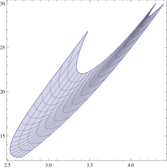
Figure 2: Parametric plot of $(\alpha_{3},\alpha_{4})$ for $a=1/2$, $b=1$ and $c\in[3/10,7/10]$, $d\in[-1,3]$.

Figure 3: Parametric plot of $(\alpha_{3},\alpha_{4})$ for $a=3/4$, $b=1$ and $c\in[3/10,7/10]$, $d\in[-1,3]$.

Figure 4: Parametric plot of $(\alpha_{3},\alpha_{4})$ for $a=-1$, $b=1$ and $c\in[1/10,9/10]$, $d\in[0,3]$.

References

- [1] Baccini, A., Barabesi, L., & Stracqualursi, L.(2016). Random variate generation and connected computational issues for the Poisson-Tweedie distribution. Computational Statistics, in press, DOI: 10.1007/s00180-015-0623-5.
- [2] Barabesi, L., Cerasa, A., Perrotta, D., & Cerioli, A. (2016). Modelling international trade data with the Tweedie distribution for anti-fraud purposes. European Journal of Operational Research, in press.
- [3] Barabesi, L., & Pratelli, L. (2014a). Discussion of “On simulation and properties of the Stable law” by L. Devroye and L. James, Statistical Methods and Applications 23, 345–351.
- [4] Barabesi, L., & Pratelli, L. (2014b). A note on a universal random variate generator for integer-valued random variables. Statistics and Computing 24, 589–596.
- [5] Barabesi, L., & Pratelli, L. (2015). Universal methods for generating random variables with a given characteristic function. Journal of Statistical Computation and Simulation 85, 1679–1691.
- [6] Christoph, G., & Schreiber, K. (1998). The generalized Linnik distributions, in Advances in Stochastic Models for Reliability, Quality and Safety (W. Kahle, E. von Collani, J. Franz and U. Jensen, eds.), Birkhuser, Boston, 3-18.
- [7] Christoph, G., & Schreiber, K. (2001). Positive Linnik and discrete Linnik distributions, in Asymptotic Methods in Probability and Statistics with Applications (N. Balakrishnan, I.A. Ibragimov and V.B. Nevzorov, eds.), Birkhuser, Boston, 3–17.
- [8] Devroye, L. (1993). A triptych of discrete distribution related to the stable law. Statistics and Probability Letters 18, 349–351.
- [9] Devroye, L. (2009). Random variate generation for exponentially and polynomially tilted stable distributions. ACM Transactions on Modeling and Computer Simulation 19, Article 18.
- [10] El-Shaarawi, A.H., Zhu, R., & Joe, H. (2011). Modelling species abundance using the Poisson-Tweedie family. Environmetrics 22, 152–164.
- [11] Gerber, H.U. (1991). From the generalized gamma to the generalized negative binomial distribution. Insurance: Mathematics and Economics 10, 303–309.
- [12] Hougaard, P. (1986). Survival models for heterogeneous populations derived from stable distributions. Biometrika 73, 387–396.
- [13] Hougaard, P., Lee, M.T., & Whitmore, G.A. (1997). Analysis of overdispersed count data by mixtures of Poisson variables and Poisson processes. Biometrics 53, 1225–1238.
- [14] Huillet, T.E. (2016). On Mittag-Leffler distributions and related stochastic processes. Journal of Computational and Applied Mathematics 296, 181–211.
- [15] Johnson, N.L., Kemp, A.W., & Kotz, S. (2005). Univariate Discrete Distributions, 3rd edn. Wiley, New York.
- [16] Jose, K.K., Uma, P., Lekshmi, V.S., & Haubold, H.J. (2010). Generalized Mittag-Leffler distributions and processes for applications in astrophysics and time series modeling, in Proceedings of the Third UN/ESA/NASA Workshop on the International Heliophysical Year 2007 and Basic Space Science, H.J. Haubold and A.M. Mathai (eds.), Springer, New York.
- [17] Kanter, M. (1975). Stable densities under change of scale and total variation inequalities, Annals of Probability 3, 697–707.
- [18] Klebanov, L.B. & Slámová, L. (2015). Tempered distributions: does universal tempering procedure exist?, arXiv:1505.02068v1[math.PR].
- [19] Linnik, Y.V. (1962). Linear forms and statistical criteria II. Translations in Mathematical Statistics and Probability 3, American Mathematical Society, Providence, 41–90.
- [20] Marcheselli, M., Baccini, A., & Barabesi, L. (2008). Parameter estimation for the discrete stable family. Communications in Statistics - Theory and Methods 37, 815–830.
- [21] Pakes, A.G. (1995). Characterization of discrete laws via mixed sums and Markov branching processes. Stochastic Processes and their Applications 55, 285–300.
- [22] Rachev, S.T., Kim, Y.S., Bianchi, M.L., & Fabozzi, F.J. (2011). Financial Models with Lévy Processes and Volatility Clustering, Wiley, New York.
- [23] Rosínski, J. (2007). Tempering stable processes. Stochastic Processes and Their Applications 117, 677–707.
- [24] Sato, K. (1999). Lévy Processes and Infinitely Divisible Distributions, Cambridge University Press, Cambridge.
- [25] xSibuya, M. (1979). Generalized hypergeometric, digamma and trigamma distributions. Annals of the Institute of Statistical Mathematics 31, 373–390.
- [26] Steutel, F.W., & van Harn, K. (1979). Discrete analogues of self-decomposability and stability, Annals of Probability 7, 893–899.
- [27] Zhu, R., & Joe, H. (2009). Modelling heavy-tailed count data using a generalized Poisson-inverse Gaussian family. Statistics & Probability Letters 79, 1695–1703.
- [28] Zolotarev, V.M. (1986). One-dimensional Stable Distributions. Translations of Mathematical Monographs 65, American Mathematical Society, Providence.