UFIFT-QG-16-02 , CCTP-2016-05

CCQCN-2016-142 , ITCP-IPP 2016/06

The Effect of Features on the Functional Form of the Scalar Power Spectrum

D. J. Brooker^1∗, N. C. Tsamis^2⋆ and R. P. Woodard^1†

¹ Department of Physics, University of Florida,
Gainesville, FL 32611, UNITED STATES

² Institute of Theoretical Physics & Computational Physics,
Department of Physics, University of Crete,
GR-710 03 Heraklion, HELLAS

ABSTRACT

We study how the scalar power spectrum of single-scalar inflation depends functionally on models with features which have been proposed to explain anomalies in the data. We exploit a new formalism based on evolving the norm-squared of the scalar mode functions, rather than the mode functions themselves.

PACS numbers: 04.50.Kd, 95.35.+d, 98.62.-g

^∗ e-mail: djbrooker@ufl.edu

^⋆ e-mail: tsamis@physics.uoc.gr

^† e-mail: woodard@phys.ufl.edu

1 Introduction

It would be difficult to over-emphasize the importance of primordial perturbations predicted by inflation [1, 2]. These are not only the first detectable quantum gravitational phenomena ever identified [3, 4, 5], they also provide the initial conditions for structure formation in the standard model of cosmology [6, 7, 8]. It is therefore frustrating, and even somewhat embarrassing, that exact results are unavailable for any realistic model of inflation, even at tree order, and even when one knows the model.

For definiteness, let us assume that inflation is described by general relativity minimally coupled to some scalar potential model,

$$\mathcal{L}=\frac{R\sqrt{-g}}{16\pi G}-\frac{1}{2}\partial_{\mu}\varphi\partial_{\nu}\varphi g^{\mu\nu}\sqrt{-g}-V(\varphi)\sqrt{-g}\;.$$ (1)

At tree order the tensor and scalar power spectra, $\Delta^{2}_{h}(k)$ and $\Delta^{2}_{\mathcal{R}}(k)$, are known in terms of the constant amplitudes approached by their mode functions, $u(t,k)$ and $v(t,k)$, after the first horizon crossing time $t_{k}$ [9],

$$\Delta^{2}_{h}(k) = \frac{k^{3}}{2\pi^{2}}\times 32\pi G\times 2\times\Bigl{|}u(t,k)\Bigr{|}^{2}_{t\gg t_{k}}\approx\frac{16GH^{2}(t_{k})}{\pi}\;,$$ (2)

$$\Delta^{2}_{\mathcal{R}}(k) = \frac{k^{3}}{2\pi^{2}}\times 4\pi G\times\Bigl{|}v(t,k)\Bigr{|}^{2}_{t\gg t_{k}}\approx\frac{GH^{2}(t_{k})}{\pi\epsilon(t_{k})}\;,$$ (3)

where $k=H(t_{k})a(t_{k})$. The problem is that we do not have exact solutions for the mode functions for realistic models of inflation, so their asymptotic values must be computed numerically. The functional forms standing to the right of expressions (2) and (3) are only the leading WKB approximations.

We use the Hubble representation [10], which is based on knowing the scale factor $a(t)$, and hence also the Hubble parameter $H(t)$ and the first slow roll parameter $\epsilon(t)$,

$$ds^{2}=-dt^{2}+a^{2}(t)d\vec{x}\!\cdot\!d\vec{x}\quad\Longrightarrow\quad H(t)\equiv\frac{\dot{a}}{a}\quad,\quad\epsilon(t)\equiv-\frac{\dot{H}}{H^{2}}\;.$$ (4)

The evolution equation, Wronskian and asymptotically early form of the tensor mode functions $u(t,k)$ are [9],

$$\ddot{u}+3H\dot{u}+\frac{k^{2}}{a^{2}}u=0\;,\;u\dot{u}^{*}\!-\!\dot{u}u^{*}=\frac{i}{a^{3}}\;,\;u(t,k)\longrightarrow\frac{\exp[-ik\int_{t_{i}}^{t}\frac{dt^{\prime}}{a(t^{\prime})}]}{\sqrt{2ka^{2}(t)}}\;.$$ (5)

The analogous relations for the scalar mode functions $v(t,k)$ are [9],

$$\ddot{v}+\Bigl{(}3H+\frac{\dot{\epsilon}}{\epsilon}\Bigr{)}\dot{v}+\frac{k^{2}}{a^{2}}v=0\;,\;v\dot{v}^{*}\!-\dot{v}v^{*}=\frac{i}{\epsilon a^{3}}\;,\;v(t,k)\longrightarrow\frac{\exp[-ik\int_{t_{i}}^{t}\frac{dt^{\prime}}{a(t^{\prime})}]}{\sqrt{2k\epsilon(t)a^{2}(t)}}\;.$$ (6)

Relations (2-3) imply that $u(t,k)$ and $v(t,k)$ approach constants after $k^{2}/a^{2}$ becomes negligible. But the only exact solutions are for $\epsilon(t)=\epsilon_{0}$,

$$u_{0}(t,k;\epsilon_{0}) \equiv \sqrt{\frac{\pi}{4(1\!-\!\epsilon_{0})H(t)a^{3}(t)}}\;H^{(1)}_{\nu_{0}}\Bigl{(}\frac{k}{(1\!-\!\epsilon_{0})H(t)a(t)}\Bigr{)}\;,\qquad$$ (7)

$$v_{0}(t,k;\epsilon_{0}) \equiv \frac{u_{0}(t,k;\epsilon_{0})}{\sqrt{\epsilon_{0}}}\qquad,\qquad\nu_{0}\equiv\frac{1}{2}\Bigl{(}\frac{3\!-\!\epsilon_{0}}{1\!-\!\epsilon_{0}}\Bigr{)}\;.$$ (8)

It is by now quite clear that no constant value of $\epsilon(t)$ is consistent with the data [16].

Although numerical methods must employed, that does not mean the best strategy is to evolve $u(t,k)$ and $v(t,k)$, or that one should abandon the goal of deriving good analytic approximations which are valid for an arbitrary inflationary geometry. We have developed a formalism for evolving the norm-squares, $M(t,k)\equiv|u(t,k)|^{2}$ and $\mathcal{N}(t,k)\equiv|v(t,k)|^{2}$, which avoids the need to keep track of the rapidly changing and irrelevant phases [17]. We have also shown that factoring out the instantaneously constant $\epsilon$ solution $u_{0}(t,k;\epsilon(t))$, and making a judicious choice of variables, gives rise to a wonderfully accurate analytic approximation for the tensor power spectrum [18, 19]. The purpose of this paper is to do the same for the scalar power spectrum.

A major issue we wish to resolve is which of the two possible approaches gives the best analytic approximation for the scalar power spectrum:

1. Exploiting the functional relation between the scalar and tensor mode functions [20, 17]; or

2. Factoring out the instantaneously constant $\epsilon(t)$ solution as we did for the tensor power spectrum [18].

In section 2 we describe these two strategies. Section 3 examines them numerically, and Section 4 discusses the results.

2 Different Strategies for Computing $\Delta^{2}_{\mathcal{R}}(k)$

Previous work has shown how relations (5-6) can be used to derive equations for the norm-squares $M(t,k)\equiv|u(t,k)|^{2}$ and $\mathcal{N}(t,k)\equiv|v(t,k)|^{2}$ [17],

$$\ddot{M}+3H\dot{M}+\frac{2k^{2}}{a^{2}}M=\frac{(\dot{M}^{2}\!+\!\frac{1}{a^{6}})}{2M} M(t,k)\longrightarrow\frac{1}{2ka^{2}(t)}\;,$$ , (9)

$$\ddot{\mathcal{N}}+\Bigl{(}3H\!+\!\frac{\dot{\epsilon}}{\epsilon}\Bigr{)}\dot{\mathcal{N}}\!+\!\frac{2k^{2}}{a^{2}}\,\mathcal{N}=\frac{(\dot{\mathcal{N}}^{2}\!+\!\frac{1}{\epsilon^{2}a^{6}})}{2\mathcal{N}} \mathcal{N}(t,k)\longrightarrow\frac{1}{2k\epsilon(t)a^{2}(t)}\;.\qquad$$ , (10)

These equations are much more efficient than (5-6) for computing the power spectra because there is no need to keep track of the irrelevant phase. (The improvement is roughly quadratic [18].) The purpose of this section is to explain the two possible strategies for further improvement in computing $\mathcal{N}(t,k)$: either by transforming $M(t,k)$ or by factoring out the instantantenously constant $\epsilon$ solution.

2.1 Transforming from Tensor to Scalar

It is important to emphasize that we are not thinking about the numerical values of the power spectra for some specific model but rather about how the power spectra depend functionally on an arbitrary inflationary expansion history $a(t)$. We use square brackets to denote this functional dependence,

$$M[a](t,k)\qquad,\qquad\mathcal{N}[a](t,k)\;.$$ (11)

It is easy to check that the tensor mode relations (5) become those of the scalar (6) under a simultaneous redefinition of “time” and of the expansion history [20, 17],

$$d\widetilde{t}\equiv\sqrt{\epsilon(t)}\,dt\qquad,\qquad\widetilde{a}(\widetilde{t})\equiv\sqrt{\epsilon(t)}\,a(t)\;.$$ (12)

The functional relation between $M$ and $\mathcal{N}$ is therefore,

$$\mathcal{N}[a](t,k)=M[\widetilde{a}](\widetilde{t},k)\;.$$ (13)

We have a good functional approximation for how the tensor power spectrum depends on a general inflationary expansion history [18]. So one might try computing $\mathcal{N}[a](t,k)$ by applying (13) to this approximate form.

In practice one would never actually solve (12) for $\widetilde{a}(\widetilde{t})$. The two geometrical quantities needed for our expression of $M[\widetilde{a}](\widetilde{t},k)$ are the Hubble parameter $\widetilde{H}(\widetilde{t})$ and the first slow roll parameter $\widetilde{\epsilon}(\widetilde{t})$. It is better to express them as functions of the untransformed time $t$, using the geometrical parameters of the original expansion history. For example, the transformed Hubble parameter is,

$$\widetilde{H}(\widetilde{t})\equiv\frac{1}{\sqrt{\epsilon(t)}}\frac{d}{dt}\ln\Bigl{[}\sqrt{\epsilon(t)}\,a(t)\Bigr{]}=\frac{H(t)}{\sqrt{\epsilon(t)}}\Bigl{[}1\!+\!\frac{\dot{\epsilon}(t)}{2\epsilon(t)H(t)}\Bigr{]}\;.$$ (14)

The corresponding transformed first slow roll parameter is,

$$\widetilde{\epsilon}(\widetilde{t})\equiv\frac{1}{\sqrt{\epsilon}}\frac{d}{dt}\Bigl{[}\frac{\sqrt{\epsilon}}{H\!+\!\frac{\dot{\epsilon}}{2\epsilon}}\Bigr{]}=\frac{\epsilon\!+\!\frac{\dot{\epsilon}}{2\epsilon H}\!+\!3(\frac{\dot{\epsilon}}{2\epsilon H})^{2}\!-\!\frac{\ddot{\epsilon}}{2\epsilon H^{2}}}{[1\!+\!\frac{\dot{\epsilon}}{2\epsilon H}]^{2}}\;.$$ (15)

Our form for $M[a](t,k)$ also requires the first and second derivatives of the transformed slow roll parameter, which can be computed by substituting expression (15) in,

$$\frac{d\widetilde{\epsilon}(d\widetilde{t})}{d\widetilde{t}}=\frac{1}{\sqrt{\epsilon(t)}}\frac{d\widetilde{\epsilon}(\widetilde{t})}{dt}\qquad,\qquad\frac{d^{2}\widetilde{\epsilon}(\widetilde{t})}{d\widetilde{t}^{2}}=\frac{1}{\sqrt{\epsilon(t)}}\frac{d}{dt}\Biggl{[}\frac{1}{\sqrt{\epsilon(t)}}\frac{d\widetilde{\epsilon}(\widetilde{t})}{dt}\Biggr{]}\;.$$ (16)

These expressions obviously involve third and fourth derivatives of $\epsilon(t)$.

Of course relation (13) is exact, so applying it to an exact result for $M[a](t,k)$ must recover $\mathcal{N}[a](t,k)$. However, what we actually have is a good approximate form for $M[a](t,k)$ [18], and our approximations for the $a(t)$ expansion history might not be so good for $\widetilde{a}(\widetilde{t})$. In particular, there are plausible models (we will study one in section 3) for which $\epsilon(t)$ is small but its first derivative can become large enough to make the factors of $[1+\frac{\dot{\epsilon}}{2\epsilon H}]$ in expressions (14-15) pass through zero. So one can see how an accurate approximation for $M[a](t,k)$ might lead to very inaccurate results for $\mathcal{N}[a](t,k)$ using relation (13).

2.2 Factoring Out $\mathcal{N}_{0}(t,k)\equiv|v_{0}(t,k,\epsilon(t))|^{2}$

A different strategy is to parallel the derivation for $M[a](t,k)$ [18]. Our technique in that case was to factor out the instantaneously constant $\epsilon(t)$ solution,

$$M(t,k)\equiv M_{0}(t,k)\!\times\!\Delta M(t,k)\qquad,\qquad M_{0}(t,k)\equiv\Bigl{|}u_{0}\Bigl{(}t,k;\epsilon(t)\Bigr{)}\Bigr{|}^{2}\;,$$ (17)

where $u_{0}(t,k;\epsilon_{0})$ is the known solution (7) for $\epsilon(t)=\epsilon_{0}$. Substituting (17) in (9) and dividing by $M(t,k)$ leads to an evolution equation for the residual $\Delta M(t,k)$,

$$\frac{\Delta\ddot{M}}{\Delta M}-\frac{1}{2}\Bigl{(}\frac{\Delta\dot{M}}{\Delta M}\Bigr{)}^{2}+\Bigl{(}3H\!+\!\frac{\dot{M}_{0}}{M_{0}}\Bigr{)}\frac{\Delta\dot{M}}{\Delta M}-\frac{1}{2a^{6}M_{0}^{2}}\Bigl{(}\frac{1}{\Delta M^{2}}\!-\!1\Bigr{)}$$ (18)

$$\hskip 113.81102pt=\frac{1}{2a^{6}M_{0}^{2}}-\frac{2k^{2}}{a^{2}}-\Bigl{[}\frac{\ddot{M}_{0}}{M_{0}}\!-\!\frac{1}{2}\Bigl{(}\frac{\dot{M}_{0}}{M_{0}}\Bigr{)}^{2}\!+\!3H\frac{\dot{M}_{0}}{M_{0}}\Bigr{]}\;.\qquad$$

One can show that the right hand side of (18) vanishes for constant $\epsilon(t)$ [18]. The next step is to convert from co-moving time $t$ to the number of e-foldings from the beginning of inflation, $n\equiv\ln[a(t)/a_{i}]$. Denoting derivatives with respect to $n$ by a prime and dividing by $H^{2}$ gives,

$$\frac{\Delta M^{\prime\prime}}{\Delta M}-\frac{1}{2}\Bigl{(}\frac{\Delta M^{\prime}}{\Delta M}\Bigr{)}^{2}+\Bigl{(}3\!-\!\epsilon\!+\!\frac{M^{\prime}_{0}}{M_{0}}\Bigr{)}\frac{\Delta M^{\prime}}{\Delta M}-\frac{1}{2H^{2}a^{6}M_{0}^{2}}\Bigl{(}\frac{1}{\Delta M^{2}}\!-\!1\Bigr{)}$$ (19)

$$\hskip 71.13188pt=\frac{1}{2H^{2}a^{6}M_{0}^{2}}-\frac{2k^{2}}{H^{2}a^{2}}-\Bigl{[}\frac{M^{\prime\prime}_{0}}{M_{0}}\!-\!\frac{1}{2}\Bigl{(}\frac{M^{\prime}_{0}}{M_{0}}\Bigr{)}^{2}\!+\!(3\!-\!\epsilon)\frac{M^{\prime}_{0}}{M_{0}}\Bigr{]}\;.\qquad$$

The many ratios in (19) suggests a change of dependent variable to $\Delta M(t,k)=\exp[-\frac{1}{2}h(n,k)]$, which implies,

$$h^{\prime\prime}-\frac{1}{4}(h^{\prime})^{2}+\Bigl{(}3\!-\!\epsilon\!+\!\frac{M^{\prime}_{0}}{M_{0}}\Bigr{)}h^{\prime}+\frac{1}{H^{2}a^{6}M_{0}^{2}}\Bigl{(}e^{h}\!-\!1\Bigr{)}=S(n,k)$$ (20)

$$\hskip 71.13188pt\equiv\frac{4k^{2}}{H^{2}a^{2}}-\frac{1}{H^{2}a^{6}M_{0}^{2}}+2\Bigl{[}\frac{M^{\prime\prime}_{0}}{M_{0}}\!-\!\frac{1}{2}\Bigl{(}\frac{M^{\prime}_{0}}{M_{0}}\Bigr{)}^{2}\!+\!(3\!-\!\epsilon)\frac{M^{\prime}_{0}}{M_{0}}\Bigr{]}\;.\qquad$$

Relation (20) is exact, but it can be easily converted to a successive approximation scheme that gives $h(n,k)$ for a general expansion history. It is useful to first take note of the relation which exists between the “frequency” and “friction” terms in (20),

$$\frac{1}{H(t)a^{3}(t)M_{0}(t,k)}\equiv\omega(n,k)\qquad\Longrightarrow\qquad 3-\epsilon+\frac{M_{0}^{\prime}}{M_{0}}=-\frac{\omega^{\prime}}{\omega}\;.$$ (21)

Now move the terms nonlinear in $h(n,k)$ from the left side of (20) to the right side,

$$h^{\prime\prime}-\frac{\omega^{\prime}}{\omega}h^{\prime}+\omega^{2}h=S(n,k)+\frac{1}{4}{h^{\prime}}^{2}+\omega^{2}\Bigl{[}1\!+\!h\!-\!e^{h}\Bigr{]}\;.$$ (22)

The left hand side of (22) is a linear differential operator acting on $h(n,k)$, whose retarded Green’s function can be written down for a general expansion history [18],

$$G(n;n^{\prime})=\frac{\theta(n\!-\!n^{\prime})}{\omega(n^{\prime},k)}\,\sin\Biggl{[}\int_{n^{\prime}}^{n}\!\!\!\!dn^{\prime\prime}\omega(n^{\prime\prime},k)\Biggr{]}\;.$$ (23)

Because $M_{0}(t,k)$ recovers the full asymptotic early time form (9), the initial conditions for $h(n,k)$ are $h(0,k)=0=h^{\prime}(0,k)$. We can use the Green’s function to express the solution to equation (22) as a series $h=h_{1}+h_{2}+\dots$ in powers of the source. The first two terms are,

$$h_{1}(n,k) = \int_{0}^{n}\!\!dn^{\prime}G(n;n^{\prime})S(n^{\prime},k)\;,$$ (24)

$$h_{2}(n,k) = \int_{0}^{n}\!\!dn^{\prime}G(n;n^{\prime})\Biggl{[}\frac{1}{4}{h_{1}^{\prime}}^{2}(n^{\prime},k)-\frac{1}{2}\omega^{2}(n^{\prime},k)h_{1}^{2}(n^{\prime},k)\Biggr{]}\;.$$ (25)

Note that the series expansion gives $h(n,k)$ as a functional of the expansion history, for a general inflationary $a(t)$. Our previous study [18] has shown that this expansion is about twice as convergent as the generalized slow roll expansion [21, 22]. Equation (22) also provides a powerful way of understanding the behavior of $h(n,k)$ as a damped, driven oscillator. The frequency term $\omega(n,k)$ in (21) is huge until just a few e-foldings before horizon crossing and then decays to zero exponentially, while the friction term is always of order one.

The review we have just presented of the tensor analysis is very relevant because the instantaneously constant $\epsilon(t)$ solution for the scalar is closely related to its tensor cousin,

$$\mathcal{N}_{0}(t,k)\equiv\Bigl{|}v_{0}\Bigl{(}t,k;\epsilon(t)\Bigr{)}\Bigr{|}^{2}=\frac{M_{0}(t,k)}{\epsilon(t)}\;.$$ (26)

If one factors this term out,

$$\mathcal{N}(t,k)\equiv\frac{M_{0}(t,k)}{\epsilon(t)}\!\times\!\Delta\mathcal{N}(t,k)\;,$$ (27)

and then divides (10) by $N(t,k)$, the resulting equation for $\Delta\mathcal{N}(t,k)$ is almost identical to (18),

$$\frac{\Delta\ddot{\mathcal{N}}}{\Delta\mathcal{N}}-\frac{1}{2}\Bigl{(}\frac{\Delta\dot{\mathcal{N}}}{\Delta\mathcal{N}}\Bigr{)}^{2}+\Bigl{(}3H\!+\!\frac{\dot{M}_{0}}{M_{0}}\Bigr{)}\frac{\Delta\dot{\mathcal{N}}}{\Delta\mathcal{N}}-\frac{1}{2a^{6}M_{0}^{2}}\Bigl{(}\frac{1}{\Delta\mathcal{N}^{2}}\!-\!1\Bigr{)}$$ (28)

$$=\frac{1}{2a^{6}M_{0}^{2}}-\frac{2k^{2}}{a^{2}}-\Bigl{[}\frac{\ddot{M}_{0}}{M_{0}}\!-\!\frac{1}{2}\Bigl{(}\frac{\dot{M}_{0}}{M_{0}}\Bigr{)}^{2}\!+\!3H\frac{\dot{M}_{0}}{M_{0}}\Bigr{]}+\frac{\ddot{\epsilon}}{\epsilon}-\frac{1}{2}\Bigl{(}\frac{\dot{\epsilon}}{\epsilon}\Bigr{)}^{2}+3H\frac{\dot{\epsilon}}{\epsilon}\;.\qquad$$

This means we can immediately read off the result of changing the independent variable to $n\equiv\ln[a(t)/a_{i}]$ and the dependent variable to $g(n,k)\equiv-2\ln[\Delta\mathcal{N}(t,k)]$,

$$g^{\prime\prime}-\frac{\omega^{\prime}}{\omega}g^{\prime}+\omega^{2}g=S(n,k)+\Delta S(n)+\frac{1}{4}{g^{\prime}}^{2}+\omega^{2}\Bigl{[}1\!+\!g\!-\!e^{g}\Bigr{]}\;.$$ (29)

Only the extra (and $k$-independent) source $\Delta S(n)$ distinguishes the scalar equation (29) from its tensor counterpart (22),

$$\Delta S(n)=-2\Biggl{[}\frac{\epsilon^{\prime\prime}}{\epsilon}-\frac{1}{2}\Bigl{(}\frac{\epsilon^{\prime}}{\epsilon}\Bigr{)}^{2}+(3\!-\!\epsilon)\frac{\epsilon^{\prime}}{\epsilon}\Biggr{]}\;.$$ (30)

It is useful to express $\Delta S(n)=\Delta S_{1}(n)+\Delta S_{2}(n)$ as the sum of a total derivative and a negative-definite term,

$$\Delta S_{1}\equiv-2\partial_{n}\Bigl{[}\partial_{n}\ln(\epsilon)\!+\!3\ln(\epsilon)\!-\!\epsilon\Bigr{]}\quad,\quad\Delta S_{2}\equiv-\Bigl{[}\partial_{n}\ln(\epsilon)\Bigr{]}^{2}\;.$$ (31)

Although $\Delta S_{1}$ is typically larger, the net impulse comes entirely from $\Delta S_{2}$.

In addition to the derivation, we can also read off the scalar asymptotic analysis from the tensor case. At early times, before horizon crossing, the frequency, friction and source take the forms [18],

$$\omega(n,k) \longrightarrow \frac{2k}{Ha}+O\Bigl{(}\frac{Ha}{k}\Bigr{)}\;,$$ (32)

$$-\frac{\omega^{\prime}(n,k)}{\omega(n,k)} \longrightarrow 1-\epsilon+O\Bigl{(}\frac{H^{2}a^{2}}{k^{2}}\Bigr{)}\;,$$ (33)

$$S(n,k) \longrightarrow -\Bigl{[}\epsilon^{\prime\prime}+(9\!-\!7\epsilon)\epsilon^{\prime}\Bigr{]}\Bigl{(}\frac{Ha}{k}\Bigr{)}^{2}+O\Bigl{(}\frac{H^{4}a^{4}}{k^{4}}\Bigr{)}\;.$$ (34)

Hence derivatives of $g(n,k)$ are irrelevant with respect to the restoring force, and the tensor source is irrelevant with respect to the extra scalar part (30),

$${\rm Early\ Times:}\quad g(n,k)=\Delta S(n)\!\times\!\Bigl{(}\frac{Ha}{2k}\Bigr{)}^{2}+O\Bigl{(}\frac{H^{4}a^{4}}{k^{4}}\Bigr{)}\;.$$ (35)

At late times, after horizon crossing, the continuing evolution of $\epsilon(t)$ causes $\mathcal{N}_{0}(t,k)$ to evolve slightly in a way that must be cancelled by continuing evolution in $g(n,k)$ in order for $\mathcal{N}(t,k)$ to approach a constant. This behavior can be described by the function $F(n,k)$ defined as [18],

$$F(n,k)\equiv\ln\Bigl{[}\frac{2(1\!-\!\epsilon)Ha}{k}\Bigr{]}+\psi\Bigl{(}\frac{1}{2}\!+\!\frac{1}{1\!-\!\epsilon}\Bigr{)}-1\;.$$ (36)

The late time forms for the frequency, friction and source are [18],

$$\omega(n,k) \longrightarrow \frac{\pi}{\Gamma(\frac{1}{2}\!+\!\frac{1}{1-\epsilon})}\Bigl{(}\frac{2k}{Ha}\Bigr{)}\Bigl{[}\frac{k}{2(1\!-\!\epsilon)Ha}\Bigr{]}^{\frac{2}{1-\epsilon}}+O\Bigl{[}\Bigl{(}\frac{k}{Ha}\Bigr{)}^{3+\frac{2}{1-\epsilon}}\Bigr{]}\;,$$ (37)

$$-\frac{\omega^{\prime}(n,k)}{\omega(n,k)} \longrightarrow \frac{2\epsilon^{\prime}F}{(1\!-\!\epsilon)^{2}}+3-\epsilon+O\Bigl{(}\frac{k^{2}}{H^{2}a^{2}}\Bigr{)}\;,$$ (38)

$$S(n,k) \longrightarrow \frac{4\epsilon^{\prime\prime}F}{(1\!-\!\epsilon)^{2}}+\frac{4\epsilon^{\prime}}{1\!-\!\epsilon}\Bigr{[}\Bigl{(}\frac{3\!-\!\epsilon}{1\!-\!\epsilon}\Bigr{)}F\!+\!1\Bigr{]}$$ (39)

$$\hskip 14.22636pt+\frac{4{\epsilon^{\prime}}^{2}}{(1\!-\!\epsilon)^{3}}\Bigl{[}\frac{F^{2}}{1\!-\!\epsilon}\!+\!2F\!-\!1\!+\!\frac{\psi(\frac{1}{2}\!+\!\frac{1}{1-\epsilon})}{1\!-\!\epsilon}\Bigr{]}+O\Bigl{(}\frac{k^{2}}{H^{2}a^{2}}\Bigr{)}\;.\qquad$$

This means the restoring force is irrelevant. Although the extra scalar source (30) does not grow, neither does it fall off, so it contributes a term to the late time behavior of $g(n,k)$, in addition to those already implied by the known form of $h(n,k)$ [18],

$${\rm Late\ Times:}\quad g(n,k)=2\ln\Biggl{[}\Bigl{(}\frac{a(t)}{a(t_{k})}\Bigr{)}^{\frac{2\epsilon(t)}{1-\epsilon(t)}}\Bigl{(}\frac{H(t)}{H(t_{k})}\Bigr{)}^{\frac{2}{1-\epsilon(t)}}\frac{C(\epsilon(t))}{C(\epsilon(t_{k})}\frac{\epsilon(t_{k})}{\epsilon(t)}\Biggr{]}$$ (40)

$$\hskip 213.39566pt-2\ln\Bigl{[}\mathcal{S}(k)\Bigr{]}+O\Bigl{(}\frac{k^{2}}{H^{2}a^{2}}\Bigr{)}\;.\qquad$$

For small $\epsilon(t)$ this extra term is enough to give $g(n,k)$ a downward slope,

$${\rm Late\ Times:}\quad g^{\prime}(n,k)=-\frac{2\epsilon^{\prime}}{\epsilon}+\frac{4\epsilon^{\prime}F}{(1\!-\!\epsilon)^{2}}+O\Bigl{(}\frac{k^{2}}{H^{2}a^{2}}\Bigr{)}\;.$$ (41)

The functions $C(\epsilon)$ and $\mathcal{S}(k)$ which appear in expression (40) show up as well in the scalar power spectrum,

$$\Delta^{2}_{\mathcal{R}}(k)=\frac{GH^{2}(t_{k})}{\pi\epsilon(t_{k})}\!\times\!C\Bigl{(}\epsilon(t_{k})\Bigr{)}\!\times\!\mathcal{S}(k)\;.$$ (42)

$C(\epsilon)$ gives all local corrections (that is, evaluated at $t=t_{k}$) to the leading slow roll approximation on the right of (3),

$$C(\epsilon)\equiv\frac{1}{\pi}\Gamma^{2}\Bigl{(}\frac{1}{2}\!+\!\frac{1}{1\!-\!\epsilon}\Bigr{)}\Bigl{[}2(1\!-\!\epsilon)\Bigr{]}^{\frac{2}{1-\epsilon}}\;.$$ (43)

The quantity $\mathcal{S}(k)$ represents the nonlocal part of the power spectrum, the need for which has long been recognized [23]. It is determined by evolving $g(n,k)$ to late times — either numerically or analytically — and then comparing with expression (40). The analytic series expansion $g=g_{1}+g_{2}+\dots$, can be developed from (29) the same way we did for the tensor case. Its first two terms are,

$$g_{1}(n,k) = \int_{0}^{n}\!\!dn^{\prime}G(n;n^{\prime})\Bigl{[}S(n^{\prime},k)+\Delta S(n)\Bigr{]}\;,$$ (44)

$$g_{2}(n,k) = \int_{0}^{n}\!\!dn^{\prime}G(n;n^{\prime})\Biggl{[}\frac{1}{4}{g_{1}^{\prime}}^{2}(n^{\prime},k)-\frac{1}{2}\omega^{2}(n^{\prime},k)g_{1}^{2}(n^{\prime},k)\Biggr{]}\;.$$ (45)

Examination of the nonlinear terms on the right hand side of equation (29) shows that the linear approximation $g(n,k)\approx g_{1}(n,k)$ can only fail under two conditions:

1. If $g^{\prime}(n,k)$ becomes order one or larger; or

2. If $g(n,k)$ becomes order one or larger during the few e-folding around horizon crossing when $\omega(n,k)$ is also of order one.

Because $g(n,k)$ is negligible before horizon crossing, the second possibility is difficult to realize, but we will see that the presence of a feature can cause the first to occur.

3 Comparing Analytic and Numerical Results

The purpose of this section is to use our formalism to study models with features. We shall mostly focus on a class of “step” models [24] whose parameters were fit to explain peculiarities in WMAP data [25]. The section accordingly begins with a review of this model. Then we contrast exact numerical simulation of its scalar power spectrum with our linearized approximation and with an improvement based on correcting the source. The evolution of a series of nine different modes is studied to develop a qualitative understanding of the “ringing” phenomenon. The section closes with a brief examination of other models with features.

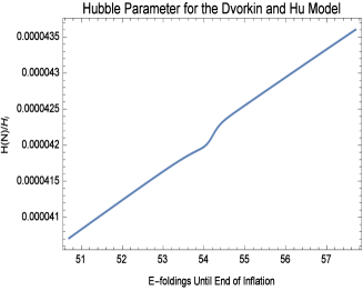
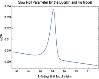
Figure 1: Graphs of the Hubble parameter and the first slow roll parameter as functions of the number of e-foldings $N\equiv n_{\rm end}-n$ until the end of inflation for the step model of section 3.1. Note that early times (large $N$) are at the right and late times (small $N$) are at the left.

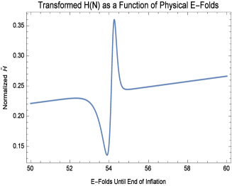
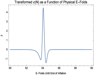
Figure 2: Graphs of the Hubble parameter $\widetilde{H}(\widetilde{t})$ (14) and the transformed first slow roll parameter $\widetilde{\epsilon}(\widetilde{t})$ (15) for the impulse model of section 3.4. These are the geometrical parameters which would be used to compute the scalar power spectrum by transforming the tensor power spectrum according to relation (13). Both graphs are expressed as functions of the number of (untransformed) e-foldings $N\equiv n_{\rm end}-n$ until the end of inflation.

3.1 The Step Model

In 2001 Adams, Cresswell and Easther proposed a generic model whose potential is quadratic with a multiplicative step of variable location, height and width [24],

$$V(\varphi)=\frac{1}{2}m^{2}\varphi^{2}\Bigl{[}1+c\tanh\Bigl{(}\frac{\varphi\!-\!b}{d}\Bigr{)}\Bigr{]}\;.$$ (46)

Features in the range $20\lesssim\ell\lesssim 40$ of the WMAP 3-year data [26, 27] were fitted to give the following maximum likelihood values for the parameters $b$, $c$, $d$ and $m$ [25],

$$b=\frac{14.668}{\sqrt{8\pi G}}\qquad \qquad c=1.505\!\times\!10^{-3}\;,$$ , (47)

$$d=\frac{0.02705}{\sqrt{8\pi G}}\qquad \qquad m=\frac{7.126\!\times\!10^{-6}}{\sqrt{8\pi G}}\;.$$ , (48)

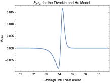
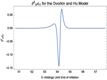
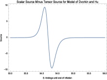
Figure 3: Graphs of $\epsilon^{\prime}$ (left), $\epsilon^{\prime\prime}$ (middle), and the extra source $\Delta S(n)$ (right) defined in equation (30) for the step model of section 3.1. In each case the functions are expressed in terms of the number of e-foldings $N\equiv n_{\rm end}-n$ until the end of inflation.

In numerically evolving this model it is best to convert to dimensionless fields and potentials,

$$\psi(n)\equiv\sqrt{8\pi G}\,\varphi(t)\qquad,\qquad U(\psi)\equiv(8\pi G)^{2}V(\varphi)\;.$$ (49)

When we also convert from co-moving time $t$ to the number of e-foldings $n\equiv\ln[a(t)/a_{i}]$, the exact scalar equation becomes,

$$\psi^{\prime\prime}+\Bigl{(}3\!-\!\frac{1}{2}{\psi^{\prime}}^{2}\Bigr{)}\psi^{\prime}+\Bigl{(}3\!-\!\frac{1}{2}{\psi^{\prime}}^{2}\Bigr{)}\frac{U^{\prime}(\psi)}{U(\psi)}=0\;.$$ (50)

The Hubble parameter and first slow roll parameter follow from $\psi(n)$ through the exact relations,

$$8\pi GH^{2}=\frac{U(\psi)}{3\!-\!\frac{1}{2}{\psi^{\prime}}^{2}}\qquad,\qquad\epsilon=\frac{1}{2}{\psi^{\prime}}^{2}\;.$$ (51)

Figure 1 shows these as functions of the number of e-foldings from the end of inflation $N\equiv n_{\rm end}-n$. Note that there is only a slight bump in the Hubble parameter, and that the first slow roll parameter remains small even though the feature does enhance it by as much as 50% over the single e-folding in the range $53.7\lesssim N\lesssim 54.7$.

Figure 2 shows transformed geometrical parameters (14-15) that would be used to obtain the scalar power spectrum by exploiting the transformation (13) from the tensor power. Note that the transformed Hubble parameter changes by almost a factor of three within a single e-folding, as the model oscillations from normal acceleration $0\leq\widetilde{\epsilon}<1$ to super-acceleration $\widetilde{\epsilon}<0$ and even deceleration $1<\widetilde{\epsilon}$. Our linearized approximation for the tensor power spectrum is very good [18], but it breaks down for such wild fluctuations. Thus we conclude that the strategy laid out in section 2.2 is better.

Figure 3 shows the first two derivatives of $\epsilon$ with respect to $n$, along with the extra scalar source $\Delta S(n)$ defined in equation (30). All functions are again displayed in terms of the number of e-foldings until the end of inflation $N\equiv n_{\rm end}-n$. A number of things are worth noting. First, the smallness of $|\partial_{n}\epsilon|<0.017$ and of $|\partial_{n}^{2}\epsilon|<0.15$ means that the tensor source $S(n,k)$ is negligible with respect to the scalar part $\Delta S(n)$ (30), whose magnitude can reach almost 10. Second, the fact that $\epsilon^{\prime\prime}$ has almost ten times the magnitude of $\epsilon^{\prime}$ means that, of the source’s two parts (31), the first one $\Delta S_{1}(n)$ totally dominates the second one $\Delta S_{2}(n)$. This is significant because $\Delta S_{1}(n)$ is a total derivative, which contributes zero net impulse after the feature has passed, whereas $\Delta S_{2}$ contributes a net negative impulse. We will see in section 4 that features for which $\Delta S_{1}(n)$ and $\Delta S_{2}(n)$ are comparable induce a qualitatively different response in $g(n,k)$ and $\Delta^{2}_{\mathcal{R}}(k)$.

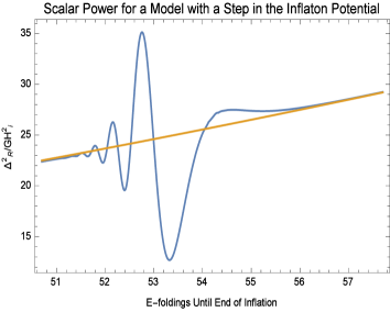
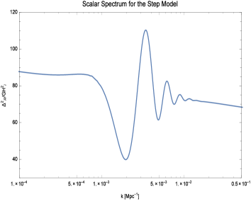
Figure 4: The left hand graph represents $\Delta^{2}_{\mathcal{R}}(k)/GH^{2}_{i}$ versus $N_{k}$, the number of e-foldings from first horizon crossing until the end of inflation. The yellow curve represents the $m^{2}\phi^{2}$ model while the blue curve shows the step model of section 3.1. The right hand graph also gives $\Delta^{2}_{\mathcal{R}}(k)/GH^{2}_{i}$, but plotted as a function of the wave number $k$.

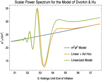
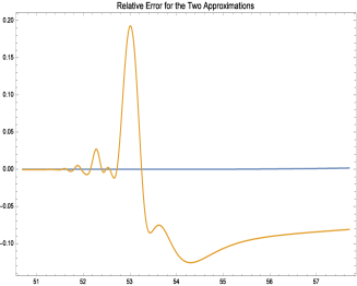
Figure 5: The left hand graph shows the linearized approximation (green) and the modified source (yellow) for the step model of section 3.1. The right hand graph shows the fractional error of our linearized approximation (yellow) and the modified source (blue).

3.2 Exact Results versus Approximations

We numerically evolved $g(n,k)$ using the exact equation (29) for the step model of section 3.1. Then the $n$-independent constant $\mathcal{S}(k)$ was inferred by comparing the late time form with expression (40), and was used in (42) to compute the scalar power spectrum. Figure 4 shows the result as a function of the number of e-foldings $N_{k}$ from the end of inflation that horizon crossing takes place. Also shown is the result for the simple quadratic potential, without the feature. Five oscillations around the nominal $m^{2}\varphi^{2}$ model are visible. They begin with a small rise in the power, beginning about an e-folding before the onset of the feature. This is followed by a much larger decrease (to as low as 50% of the $m^{2}\varphi^{2}$ amplitude), starting in the midpoint of the feature and extending about half an e-folding beyond. Each subsequent fluctuation is smaller, with the frequency of oscillation also decreasing. The ringing persists for about two e-foldings after the feature has passed.

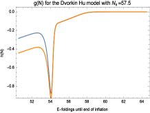
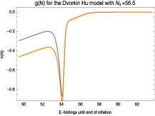
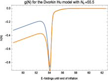
Figure 6: Graphs of our linearized approximation $g(n,k)\approx g_{1}(n,k)$ (yellow) versus the full result (in blue) for the step model of section 3.1 at very early horizon crossing times. Shown are $N_{k}=57.5$ (left), $N_{k}=56.5$ (middle) and $N_{k}=55.5$ (right). After horizon crossing the full $g(n,k)$ assumes a downward sloping decline which the feature temporarily disturbs and also introduces a further, and incorrect, downward offset.

Understanding the ringing merits a sub-section of its own, but let us first consider the accuracy of the linearized approximation $g(n,k)\approx g_{1}(n,k)$ defined in expression (44). Figure 5 displays the linearized approximation, as well as its fractional error. All of the oscillations are present, at about the right places, and the 20% maximum error is about what Dvorkin and Hu found using a second order generalized slow roll expansion based on the mode functions [22]. Also shown in Figure 5 is the effect of including a simplified form of $g_{2}(n,k)$ in which only the asymptotic form (41) for $g^{\prime}(n,k)$ is used in expression (45). This might be termed the “1.5 order approximation”, and it is so good that one’s eye cannot distinguish it from the exact curve.

One disturbing thing of the linearized approximation is the systematic enhancement of the power spectrum for modes which experience horizon crossing before the feature. This can be clearly seen in Figure 5. The fact that this problem disappears from the 1.5 order approximation signals its origin from the feature causing $g^{\prime}(n,k)$ to become significant. Figure 6 shows what is going on with the full $g(n,k)$ for three modes which experience horizon crossing before the onset of the feature. After horizon crossing, and before the feature, these modes have settled into the asymptotic form predicted by expression (41), with the slight downward slope caused by the continuing growth of $\epsilon$ in the $m^{2}\varphi^{2}$ model. Then the feature induces a rapid fall and rise of $g(n,k)$, which makes the $\frac{1}{4}{g^{\prime}}^{2}$ term on the right hand side of (29) impart a positive impulse to $g(n,k)$. Neglecting this term — which the linearized approximation does — results in $g_{1}(n,k)$ being more negative than $g(n,k)$, and hence in the power spectrum of the linearized model having a greater amplitude than it should.

3.3 Understanding the Ringing

Figure 4 of the scalar power spectrum for the step model displays four striking properties we seek to understand:

1. As the time of horizon crossing is made later, the power is alternatively enhanced or suppressed, with respect to the $m^{2}\varphi^{2}$ model on which the feature was imposed, with progressively decreasing amplitude;

2. As the time of horizon crossing is made later, the period of oscillation decreases, significantly for early horizon crossings, but only slightly for late horizon crossings;

3. Modes which experience horizon crossing near the end of the feature and just afterwards show a large suppression of power; and

4. Modes which experience horizon crossing before the onset of the feature show a slight enhancement.

Of course the value of the power spectrum for a given wave number $k$ depends on the asymptotic form of $g(n,k)$, through relations (40) and (42). However, what asymptotic form is reached depends on the previous evolution, and we can understand that evolution by thinking about $g(n,k)$ as a damped, driven oscillator whose restoring force is huge before horizon crossing and then rapidly drops away while friction persists.

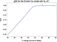
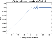
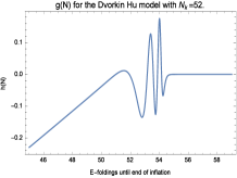
Figure 7: Graphs of $g(n,k)$ for the step model of section 3.1 for horizon crossing times after the end of the feature. Shown are the evolutions (early to the right and late to the left) for horizon crossings at $N_{k}=51.0$ (left), $N_{k}=51.5$ (middle) and $N_{k}=52.0$ (right).

The driving force consists principally of $\Delta S(n)$, which acts between $53.7\lesssim N\lesssim 54.7$. Much depends on when horizon crossing occurs with respect to that interval. Figure 7 displays $g(n,k)$ for three values of $N_{k}$ which occur after the feature. In this case the restoring force is huge during the lifetime of the feature, so $g(n,k)$ tracks the driving force according to relation (35). For the latest horizon crossing ($N_{k}=51.0$) there is only this single oscillation. However, when horizon comes at $N_{k}=51.5$, the restoring force has declined and we begin to see subsequent oscillations which result from the oscillator responding to the net negative impulse imparted by $\Delta S_{2}(n)=-[\epsilon^{\prime}/\epsilon]^{2}$. These oscillations stop slightly before horizon crossing because the restoring force is no longer present. By $N_{k}=52.0$ the restoring force is correspondingly smaller during the lifetime of the feature, which makes the amplitude of fluctuation larger. However, there is less time before the restoring force dies away, so there are fewer fluctuations. One can also note that the period of oscillation increases.

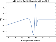
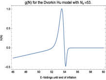
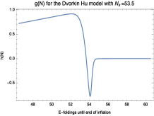
Figure 8: Graphs of $g(n,k)$ for the step model of section 3.1 for horizon crossing times shortly after the end of the feature (at $N\approx 53.7$. Shown are the evolutions (early to the right and late to the left) for horizon crossings at $N_{k}=52.5$ (left), $N_{k}=53.0$ (middle) and $N_{k}=53.5$ (right).

All of these trends are continued for the sequence of evolutions shown in Figure 8 for modes which experience horizon crossing shortly after the end of the feature. For these modes the restoring force is smaller during the lifetime of the feature, which makes for fluctuations of larger amplitude. However, the restoring force also disappears sooner, which makes for fewer oscillations. The case of $N_{k}=52.5$ shows two troughs and one peak, while $N_{k}=53.0$ has one trough and one peak, and $N_{k}=53.5$ has only a single trough.

A little reflection reveals that we have the explanation for the first property of Figure 4. The value of the power spectrum for any $k$ depends on the asymptotic form (40) reached by $g(n,k)$. At fixed $k$, this asymptotic form is determined by where $g(n,k)$ is in the sequence of oscillations caused by the feature, when the restoring force turns off. For some values of $k$ that point comes when $g(n,k)$ is in a trough, for other values of $k$ the restoring force turns off when $g(n,k)$ is at a peak. That is why there are fluctuations. The amplitude of fluctuation becomes smaller for later horizon crossing because the restoring force at the time of the feature is correspondingly larger.

The second property, concerning the period of oscillation, has a more complicated explanation associated with the nonlinear terms in equation (29) for $g(n,k)$. The actual restoring force is $\omega^{2}[e^{g}-1]$, so positive values of $g(n,k)$ increase it, with respect to the linear approximation, while negative values of $g(n,k)$ decrease it. The system tends to spend a little less time on upward fluctuations, and a little more on downwards ones, with the net effect a lengthening of the period for one full oscillation. One can see from Figure 8 that the amplitude of $g(n,k)$ becomes large enough to make the oscillator significantly anharmonic. The later horizon crossing times of Figure 7 never reach such large amplitudes, which is why the period of fluctuations on Figure 4 decreases as $N_{k}$ becomes smaller.

Property 3, the large enhancement for modes which experience horizon crossing near the end of the feature, is shown by the final graph on Figure 8. For $N_{k}=53.5$ the restoring force is of order one just a little after the feature has ended. The restoring force turns off just as the system is rebounding, whereupon it continues to drift upwards until stopped by friction. Positive $g(n,k)$ means $\Delta\mathcal{N}(t,k)=\exp[-\frac{1}{2}g(n,k)]$ is decreased, so the power should be reduced, which is what one sees on Figure 4.

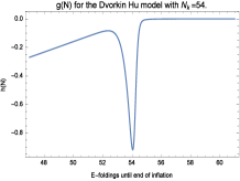
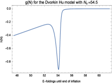
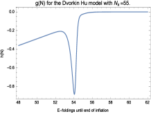
Figure 9: Graphs of $g(n,k)$ for the step model of section 3.1 for horizon crossing times during and slightly before the onset of the feature. Shown are the evolutions (early to the right and late to the left) for horizon crossings at $N_{k}=54.0$ (left), $N_{k}=54.5$ (middle) and $N_{k}=55.0$ (right).

Figure 9 shows three modes whose horizon crossing times occur during and slightly before the feature. For these modes the restoring force is nearly absent during the lifetime of the feature so what one sees is the effect of the driving force on a massless particle with friction. The driving force $\Delta S(n)$ (30) is depicted on the right hand side of Figure 3. Without friction it would first push $g(n,k)$ negative and then pull it back up. With friction, and the small negative impulse imparted by $\Delta S_{2}(n)$ (31), one can see that $g(n,k)$ will not quite reach equilibrium, and this is reflected in Figure 9. The result is to make $g(n,k)$ more negative than it would have been without the feature, which increases $\Delta\mathcal{N}(t,k)=\exp[-\frac{1}{2}g(n,k)]$. The net effect on the power spectrum is decreased because these modes come during the lifetime of the feature. One can see from Figure 1 that the factor of $1/\epsilon(t_{k})$ in (42) is decreased. That is why the peak on the right of Figure 4 is shallow.

3.4 The Impulse Model

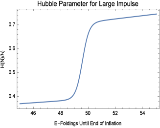
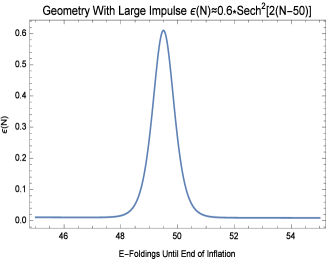
Figure 10: Graphs of the Hubble parameter and the first slow roll parameter as functions of the number of e-foldings $N\equiv n_{\rm end}-n$ until the end of inflation for the impulse model of section 3.4. Note that the passage of the feature causes a large reduction in the Hubble parameter.

Recall that the extra scalar source (30) can be decomposed into two parts (31): a total derivative $\Delta S_{1}(n)$ and a negative-definite part $\Delta S_{2}(n)$ which contributes the net impulse. is negative-definite. The step model typifies features for which $|\Delta S_{1}(n)|\gg|\Delta S_{2}(n)|$, and the response we saw in sections 3.2 and 3.3 is generic. It is difficult to make $\Delta S_{2}(n)$ dominate $\Delta S_{1}(n)$ for very long, but there is another class of features for which the two terms are comparable, and this class shows a very different response.

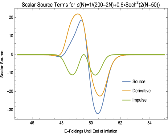
Figure 11: Graphs of the scalar source for the model (52-53) of section 3.4. Shown are $\Delta S(n)$ (blue), $\Delta S_{1}(n)$ (orange) and $\Delta S_{2}(n)$ (green).

One can make $\Delta S_{1}(n)$ and $\Delta S_{2}(n)$ comparable by causing the peak value of $\epsilon$ at the feature to be much larger than the background on which it is imposed. As an example, consider the model defined by,

$$\epsilon(n)=\frac{1}{200\!-\!2n}+\frac{3}{5}\,{\rm sech}^{2}\Bigl{[}2(n\!-\!50)\Bigr{]}\;.$$ (52)

The associated Hubble parameter is,

$$H(n)=H_{i}\sqrt{1\!-\!\frac{n}{100}}\,\exp\Biggl{[}-\frac{3}{10}\!-\!\frac{3}{10}\tanh\Bigl{[}2(n\!-\!50)\Bigr{]}\Biggr{]}\;.$$ (53)

Figure 10 displays (52-53). Note that the feature effectively persists from $N\equiv n_{\rm end}-n\simeq 51.5$ to $N\simeq 48.0$, so it is much broader than the step model. Note also that the passage of the feature reduces $H^{2}$ by about a factor of two, whereas the step model of section 3.1 shows hardly any change. Figure 11 displays $\Delta S(n)$ and its two parts. Note that the magnitude of $\Delta S_{2}$ is only a factor of two smaller than that of $\Delta S_{1}$, whereas the magnitudes differ by a factor of ten for the step model.

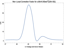
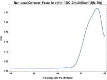
Figure 12: The left hand graph shows $\Delta^{2}_{\mathcal{R}}(k)/GH_{i}^{2}$ for the impulse model of section 3.4. The middle and right hand graphs show the nonlocal factor $\mathcal{S}(k)$ for this model. All graphs are displayed as function of $N_{k}$, the number of e-foldings between horizon crossing and the end of inflation.

Figure 12 shows the scalar power spectrum for the impulse model. Also displayed is the nonlocal factor $\mathcal{S}(k)$ from our representation (42). Recall that $\mathcal{S}(k)$ is the part of the power spectrum which is not attributable to local changes of the geometry at the time of horizon crossing. The feature is so big in this model that the largest fluctuation of $\Delta^{2}_{\mathcal{R}}(k)$ derives from changes in the leading slow roll approximation, $GH^{2}(t_{k})/\pi\epsilon(t_{k})$. That is what suppresses the power so much in the range $49.0\lesssim N_{k}\lesssim 50.5$. However, there are also quite large effects from $\mathcal{S}(k)$, including the big bump in the region $48.5\lesssim N_{k}\lesssim 49.5$ and the smaller bump in the range $50.0\lesssim N_{k}\lesssim 50.7$. The feature of this model is so broad that much of its impulse is dissipated during the feature, and subsequent ringing is less than for the step model.

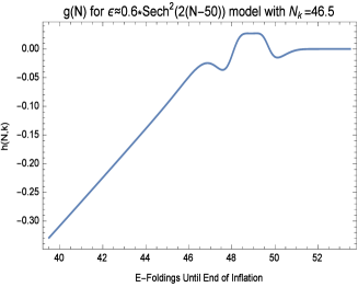
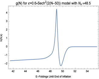
Figure 13: Graphs of $g(n,k)$ for the impulse model of section 3.4 for two modes which experience horizon crossing after (on the right) and near the end of (on the left) the feature. Both curves are displayed as functions of $N\equiv n_{\rm end}-n$, the number of e-foldings until the end of inflation.

Figure 13 shows the evolution of $g(n,k)$ for two modes which experience horizon crossing after, and near the end of, the feature. In the first case ($N_{k}=46.5$) the restoring force is still significant during the feature, which suppresses the response. It is worthwhile comparing this evolution with that depicted on the far right of Figure 7 for a mode which experiences horizon crossing about the same number of e-foldings after the feature of the step model. Although $g(n,k)$ is quite different during the feature — because the sources are different — the subsequent evolution is quite similar. For the second of the Figure 13 graphs ($N_{k}=48.5$) the initial, downward push from the source is suppressed by the still significant restoring force, but the final, upward push is unsuppressed as the restoring force dissipates. The large values of $g(n,k)$ mean that nonlinear effects are significant.

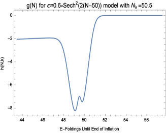
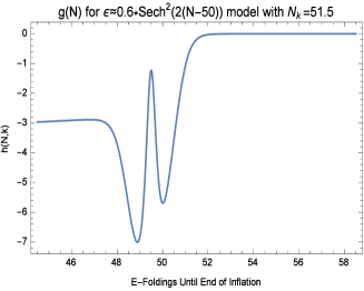
Figure 14: Graphs of $g(n,k)$ for the impulse model of section 3.4 for two modes which experience horizon crossing during the passage of the feature. Both curves are displayed as functions of $N\equiv n_{\rm end}-n$, the number of e-foldings until the end of inflation.

Figure 14 shows $g(n,k)$ for two modes which experience horizon crossing during the first part of the feature. In both cases $g(n,k)$ is pushed in the negative direction due to the net negative impulse which is imparted by $\Delta S_{2}(n)$. Because the feature of the impulse model is so much larger than that of the step model, both of these modes are pushed into the nonlinear regime. In both cases, one can note rebounds at $N=49.5$, corresponding to where $\Delta S_{2}(n)$ vanishes. For the earlier horizon crossing ($N_{k}=51.5$) this rebound is quite prominent, presumably because the restoring force is small.

4 Epilogue

Our goal is to understand how the scalar and tensor power spectra depend functionally on the expansion history of inflation. That is, we wish to express them as functionals of $a(t)$ for a general inflationary expansion history. A previous study [18] developed such a representation for the tensor power spectrum based on first deriving an evolution equation (9) for the norm-squared of the tensor mode function [17], then factoring out the instantaneously constant $\epsilon$ solution (17), and finally recognizing that the exact equation (22) for the residual factor has a series solution based on an explicit Green’s function (23). This expansion is so good that only the first term (24) is needed for normal models [18].

The goal of this paper was to develop a functional representation for the scalar power spectrum. Two competing strategies were described in section 2: either exploit the exact functional relation (13) between the tensor and scalar power spectra, or else parallel the tensor analysis by factoring out the instantaneously constant $\epsilon$ solution. Of course the transformation (13) is exact, and would be effective if used on the exact tensor power spectrum. However, our numerical studies of section 3 show that it does not give accurate results when used on our linearized approximation. The reason is that the presence of even small features in the original expansion history induces wild behavior in the transformed geometry required to employ relation (13). From Figure 2 one can see that even models which have been fitted to real data [25] cause the transformed geometry to oscillate between normal acceleration ($0\leq\widetilde{\epsilon}<1$ to deceleration ($1<\widetilde{\epsilon}$) and even super-acceleration ($\widetilde{\epsilon}<0$). Although our analytic approximation for the tensor power spectrum is very good [18], it breaks down for such violent fluctuations.

The more effective strategy is factoring out the instantaneously constant $\epsilon$ solution as described in section 2.2. One surprise is that the final evolution equation (29) differs from its tensor cousin (22) only by the addition of a few terms (30). In particular, the Green’s function (23) is identical, and the series solution (44-45) differs only by the inclusion of this extra source in the first term. This allowed us to largely read off the asymptotic behaviors (35) and (40) from our previous tensor study [18].

$\Delta^{2}_{\mathcal{R}}(k)$ takes the form (42) of a leading slow roll approximation, times a function (43) of the slow roll parameter at horizon crossing, times a nonlocal functional $\mathcal{S}(k)$ which depends upon times before and after horizon crossing. One computes this last factor by solving for the residual $g(n,k)$ — either numerically from (29), or else by using our series expansion (44-45) — then comparing with the late time asymptotic form (40).

It is useful to think about the scalar residual $g(n,k)$ as a damped, driven oscillator in the same way we previously developed for the tensor residual $h(n,k)$ [18]. Comparison of the tensor equation (22) with its scalar cousin (29) reveals that both residuals experience the same restoring force and the same friction, and both oscillators are disrupted by the same nonlinear terms. The initial restoring force is exponentially huge, becomes of order one at horizon crossing, and dies away after that with exponential swiftness. In contrast, the friction term is always of order one. This means that the driving force can only become effective a few e-foldings before horizon crossing. If it gives the system a sufficiently large kick during that time, there will be a series of oscillations of decreasing frequency as the restoring force dies away and friction damps the motion. However, it is important to understand that the power spectra do not directly reflect these oscillations, only their effect on the asymptotic amplitudes of the mode functions.

The only difference between the scalar equation (29) and the tensor one (22) is the presence of an extra driving force $\Delta S(n)$ for the scalar. Both the tensor driving force $S(n,k)$ and the extra scalar part $\Delta S(n)$ are proportional to the first and second derivatives of the first slow roll parameter $\epsilon$. However, $\Delta S(n)$ tends to be much larger because it involves factors of $1/\epsilon$ which $S(n,k)$ lacks. This means that the scalar response to a feature is much larger than the tensor response. It also comes sooner because $S(n,k)$ is negligible before horizon crossing, which is not necessarily true for $\Delta S(n)$.

Two classes of models differ by the relation between the two parts (31) of the scalar source (30). For the step model of section 3.1 the magnitude of $\Delta S_{1}(n)$ is about ten times that of $\Delta S_{2}(n)$, whereas the two parts are comparable, and the feature is much broader, for the impulse model of section 3.4. The resulting, very different, power spectra are shown for the step model in Figure 4 and for the impulse model in Figure 12.

Although the power spectra depend only on the norm-squared of the mode functions, other quantities depend upon the phase, such as non-Gaussianities and the propagators for the $h_{ij}$ and $\zeta$ fields. We might define the full tensor and scalar mode functions as,

$$u(t,k)\equiv\sqrt{M(t,k)}\!\times\!e^{-i\theta(t,k)}\qquad,\qquad v(t,k)\equiv\sqrt{\mathcal{N}(t,k)}\!\times\!e^{-i\phi(t,k)}\;.$$ (54)

Our work so far has been to develop good analytic expressions for $M(t,k)$ and $\mathcal{N}(t,k)$, but it is simple to use the Wronskians to express the phases in terms of the magnitudes,

$$u\dot{u}^{*}-\dot{u}u^{*}=\frac{i}{a^{3}}\qquad \Longrightarrow \qquad\dot{\theta}(t,k)=\frac{1}{2a^{3}(t)M(t,k)}\;,$$ (55)

$$v\dot{v}^{*}-\dot{v}v^{*}=\frac{i}{\epsilon a^{3}}\qquad \Longrightarrow \qquad\dot{\phi}(t,k)=\frac{1}{2\epsilon(t)a^{3}(t)\mathcal{N}(t,k)}\;.$$ (56)

Expressions (55-56) mean that no extra work is needed to obtain the full mode functions. They also explain the early time expansions for $M(t,k)$ and $\mathcal{N}(t,k)$ are local (for example, equation (35)) while the phases are not (for example, the right hand sides of equations (5-6)). And they limit the degree of nonlocality — in addition the that which may be present in the magnitudes — to just a single integral. That is especially important for the products of mode functions at different times which enter both the propagator and the tree order non-Gaussianity,

$$u(t,k)u^{*}(t^{\prime},k) = \sqrt{M(t,k)M(t^{\prime},k)}\,\exp\Bigl{[}-i\!\!\int_{t^{\prime}}^{t}\!\!\frac{dt^{\prime\prime}}{2a^{3}(t^{\prime\prime})M(t^{\prime\prime},k)}\Bigr{]}\;,$$ (57)

$$v(t,k)v^{*}(t^{\prime},k) = \sqrt{\mathcal{N}(t,k)\mathcal{N}(t^{\prime},k)}\,\exp\Bigl{[}-i\!\!\int_{t^{\prime}}^{t}\!\!\frac{dt^{\prime\prime}}{2\epsilon(t^{\prime\prime})a^{3}(t^{\prime\prime})\mathcal{N}(t^{\prime\prime},k)}\Bigr{]}\;.\qquad$$ (58)

Finally, we return to a question about the $\zeta$ propagator $i\Delta(t_{1},\vec{x}_{1};t_{2},\vec{x}_{2})$ which was raised in our tensor study [18]. One can tell from the case of constant $\epsilon(t)$ that this propagator must contain a factor of “$1/\epsilon$”. However, it has never been clear at what time, or times, that factor should be evaluated. In particular, might it come from from some time far to the past of $t_{1}$ and $t_{2}$, when $\epsilon(t)$ was much smaller than either $\epsilon(t_{1})$ or $\epsilon(t_{2})$? For the sake of simplicity let us assume $t_{1}>t_{2}$, in which case the $\zeta$ propagator is,

$$i\Delta(t_{1},\vec{x}_{1};t_{2},\vec{x}_{2})=\int\!\!\frac{dk}{k}\frac{\sin(k\Delta x)}{k\Delta x}\!\times\!\frac{k^{3}}{2\pi^{2}}\,v(t_{1},k)v^{*}(t_{2},k)\;,$$ (59)

where $\Delta x\equiv\|\vec{x}_{1}-\vec{x}_{2}\|$. For sub-horizon wave numbers $k>H(t)a(t)$ our analysis shows that the amplitude of the full mode function $v(t,k)$ closely tracks that of the instantaneously constant $\epsilon$ solution $v_{0}(t,k;\epsilon(t))$ (8). Expression (35) also shows that even the corrections to $v_{0}(t,k;\epsilon(t))$ are both exponentially suppressed and local for sub-horizon modes. Memories of earlier times only begin to have an effect a few e-foldings before horizon crossing.

Super-horizon modes behave quite differently. Their amplitudes freeze into to the values they held near the time of first horizon crossing,

$$k\ll H(t_{2})a(t_{2})\quad\Longrightarrow\quad\frac{k^{3}}{2\pi^{2}}v(t_{1},k)v^{*}(t_{2},k)\approx\frac{H^{2}(t_{k})}{4\pi^{2}\epsilon(t_{k})}\!\times\!C\Bigl{(}\epsilon(t_{k})\Bigr{)}\!\times\!\mathcal{S}(k)\;.$$ (60)

Of course the propagator (59) consists of a sum over all modes, so the super-horizon modes can indeed depend upon times far in the past of either $t_{1}$ or $t_{2}$, when $\epsilon(t_{k})$ was smaller and $H(t_{k})$ was larger. Because $C(\epsilon)$ is a monotonically decreasing function of $\epsilon$, smaller $\epsilon(t_{k})$ makes this factor closer to its maximum value of one [18]. Our analysis shows that the nonlocal factor $\mathcal{S}(k)$ can indeed be significant if the model possesses a feature, but the effect will be limited to only a few e-foldings of the horizon crossing time.

Acknowledgements

This work was partially supported by the European Union’s Seventh Framework Programme (FP7-REGPOT-2012-2013-1) under grant agreement number 316165; by the European Union’s Horizon 2020 Programme under grant agreement 669288-SM-GRAV-ERC-2014-ADG; by a travel grant from the University of Florida International Center, College of Liberal Arts and Sciences, Graduate School and Office of the Provost; by NSF grant PHY-1506513; and by the UF’s Institute for Fundamental Theory. One of us (NCT) would like to thank AEI at the University of Bern for its hospitality while this work was partially completed.

References

- [1] A. A. Starobinsky, JETP Lett. 30, 682 (1979) [Pisma Zh. Eksp. Teor. Fiz. 30, 719 (1979)].
- [2] V. F. Mukhanov and G. V. Chibisov, JETP Lett. 33, 532 (1981) [Pisma Zh. Eksp. Teor. Fiz. 33, 549 (1981)].
- [3] R. P. Woodard, Rept. Prog. Phys. 72, 126002 (2009) doi:10.1088/0034-4885/72/12/126002 [arXiv:0907.4238 [gr-qc]].
- [4] A. Ashoorioon, P. S. Bhupal Dev and A. Mazumdar, Mod. Phys. Lett. A 29, no. 30, 1450163 (2014) doi:10.1142/S0217732314501636 [arXiv:1211.4678 [hep-th]].
- [5] L. M. Krauss and F. Wilczek, Phys. Rev. D 89, no. 4, 047501 (2014) doi:10.1103/PhysRevD.89.047501 [arXiv:1309.5343 [hep-th]].
- [6] V. F. Mukhanov, H. A. Feldman and R. H. Brandenberger, Phys. Rept. 215, 203 (1992). doi:10.1016/0370-1573(92)90044-Z
- [7] A. R. Liddle and D. H. Lyth, Phys. Rept. 231, 1 (1993) doi:10.1016/0370-1573(93)90114-S [astro-ph/9303019].
- [8] S. Dodelson, Amsterdam, Netherlands: Academic Pr. (2003) 440 p
- [9] R. P. Woodard, Int. J. Mod. Phys. D 23, no. 09, 1430020 (2014) doi:10.1142/S0218271814300201 [arXiv:1407.4748 [gr-qc]].
- [10] A. R. Liddle, P. Parsons and J. D. Barrow, Phys. Rev. D 50, 7222 (1994) doi:10.1103/PhysRevD.50.7222 [astro-ph/9408015].
- [11] N. C. Tsamis and R. P. Woodard, Annals Phys. 267, 145 (1998) doi:10.1006/aphy.1998.5816 [hep-ph/9712331].
- [12] T. D. Saini, S. Raychaudhury, V. Sahni and A. A. Starobinsky, Phys. Rev. Lett. 85, 1162 (2000) doi:10.1103/PhysRevLett.85.1162 [astro-ph/9910231].
- [13] S. Capozziello, S. Nojiri and S. D. Odintsov, Phys. Lett. B 634, 93 (2006) doi:10.1016/j.physletb.2006.01.065 [hep-th/0512118].
- [14] R. P. Woodard, Lect. Notes Phys. 720, 403 (2007) doi:10.1007/978-3-540-71013-4_14 [astro-ph/0601672].
- [15] Z. K. Guo, N. Ohta and Y. Z. Zhang, Mod. Phys. Lett. A 22, 883 (2007) doi:10.1142/S0217732307022839 [astro-ph/0603109].
- [16] P. A. R. Ade et al. [Planck Collaboration], arXiv:1502.02114 [astro-ph.CO].
- [17] M. G. Romania, N. C. Tsamis and R. P. Woodard, JCAP 1208, 029 (2012) doi:10.1088/1475-7516/2012/08/029 [arXiv:1207.3227 [astro-ph.CO]].
- [18] D. J. Brooker, N. C. Tsamis and R. P. Woodard, Phys. Rev. D 93, no. 4, 043503 (2016) doi:10.1103/PhysRevD.93.043503 [arXiv:1507.07452 [astro-ph.CO]].
- [19] D. J. Brooker, N. C. Tsamis and R. P. Woodard, arXiv:1603.06399 [astro-ph.CO].
- [20] N. C. Tsamis and R. P. Woodard, Class. Quant. Grav. 21, 93 (2003) doi:10.1088/0264-9381/21/1/007 [astro-ph/0306602].
- [21] E. D. Stewart, Phys. Rev. D 65, 103508 (2002) doi:10.1103/PhysRevD.65.103508 [astro-ph/0110322].
- [22] C. Dvorkin and W. Hu, Phys. Rev. D 81, 023518 (2010) doi:10.1103/PhysRevD.81.023518 [arXiv:0910.2237 [astro-ph.CO]].
- [23] L. M. Wang, V. F. Mukhanov and P. J. Steinhardt, Phys. Lett. B 414, 18 (1997) doi:10.1016/S0370-2693(97)01166-0 [astro-ph/9709032].
- [24] J. A. Adams, B. Cresswell and R. Easther, Phys. Rev. D 64, 123514 (2001) doi:10.1103/PhysRevD.64.123514 [astro-ph/0102236].
- [25] M. J. Mortonson, C. Dvorkin, H. V. Peiris and W. Hu, Phys. Rev. D 79, 103519 (2009) doi:10.1103/PhysRevD.79.103519 [arXiv:0903.4920 [astro-ph.CO]].
- [26] L. Covi, J. Hamann, A. Melchiorri, A. Slosar and I. Sorbera, Phys. Rev. D 74, 083509 (2006) doi:10.1103/PhysRevD.74.083509 [astro-ph/0606452].
- [27] J. Hamann, L. Covi, A. Melchiorri and A. Slosar, Phys. Rev. D 76, 023503 (2007) doi:10.1103/PhysRevD.76.023503 [astro-ph/0701380].