Transport of Correlations in a Harmonic Chain

Abstract

We study the propagation of different types of correlations through a quantum bus formed by a chain of coupled harmonic oscillators. This includes steering, entanglement, mutual information, quantum discord and Bell-like nonlocality. The whole system consists of the quantum bus (propagation medium) and other quantum harmonic oscillators (sources and receivers of quantum correlations) weakly coupled to the chain. We are particularly interested in using the point of view of transport to spot distinctive features displayed by different kinds of correlations. We found, for instance, that there are fundamental differences in the way steering and discord propagate, depending on the way they are defined with respect to the parties involved in the initial correlated state. We analyzed both the closed and open system dynamics as well as the role played by thermal excitations in the propagation of the correlations.

I Introduction

A direct consequence of the inherent probabilistic nature of measurement outputs and state superposition of the quantum world is the existence of correlations that can not be explained through a classical description. Although most of these correlations have been well studied gisin ; horodeckis ; amico ; jones ; ollivier ; henderson ; groisman ; wiseman , their features in the problem of transport are yet not fully explored in the literature, except for a few exceptional cases plenio2004 ; plenio2005 . It is still missing, however, a comparative study dedicated to contrast the way different correlations are transported in a chain of coupled quantum systems. The present work is dedicated to this matter. This kind of study recognizes that a fundamental requisite to perform quantum communication is precisely the ability to move information/correlations around quantum systems, and tries to use this paradigm to compare different correlations as propagation is involved.

The propagation of entanglement through harmonic networks is one of the few examples which are well explored in the literature in plenio2004 ; plenio2005 . Notably, in plenio2005 a useful scheme for high efficiency entanglement propagation, under unitary dynamics (closed system), is developed for a linear chain. The proposed method consists of minimal adjustments of frequencies and coupling constants to boost the efficiency. The result is that the chain is transformed in a quantum bus able to distribute entanglement among quantum systems coupled to it. To understand this result, a simple yet accurate model obtained using the rotating wave approximation (RWA) is employed. In nicacio4 , symplectic tools are used to generalize this approach and to arrive at an effective and accurate simple description suitable for arbitrary topologies (beyond linear chains) and open system dynamics (interaction with environment).

The main goal of our present work is to apply the system described in plenio2005 to the study of transport of different quantum correlations, not only entanglement. We are interested, for instance, in how an intrinsically asymmetric correlation such as quantum steering propagates. It is well known that given a state of a composed system $A\otimes B$, steering $AB$ may be different than steering $BA$ jones ; wiseman . How does this difference show up in a propagation problem? For our knowledge, it is the first time steering is studied under this perspective. Additionally, we do not restrict our investigation to entanglement and steering as we also include propagation of discord ollivier ; henderson , mutual information henderson ; groisman and Bell-like nonlocality jones ; wiseman ; gisin to end up with a broad view of the propagations of quantum correlations using a quantum bus. We also include the action of thermal baths to mimic the effects of losses during the transmission of the correlations. For that, we apply the method developed in nicacio4 to arrive at an effective description of the system dynamics which allowed us to obtain physically relevant analytical expressions to explain the main features of the propagation problem. Numerical solutions of the exact equations of motion are also always employed to support the validity of the analytical treatment.

The question of how such different types of correlation propagate in a chain of coupled quantum systems is by itself a question of theoretical relevance. However, it goes beyond that since moving correlations around in large systems seems to be relevant to the successful use of quantum information in practical terms. Today, we see an unprecedented level of control over nano- and mesoscopic systems where such an ability to propagate correlations may be required in near future. In this scope, the harmonic movement of interacting nanoelectromechanical oscillators buks and systems consisting of dipole-dipole interacting trapped ions bermudez are illustrative examples.

This article is organized as follows. In Sec. II, we describe the physical setup used in this work. This includes the quantum bus plenio2005 , used to establish correlations among external oscillators attached to it, and the procedure put forward in nicacio4 to treat the open system case. In Sec.  III, we review the concepts that motivate the definition of the different correlations used in this work and particularize them to the bipartite Gaussian-state scenario. The propagation phenomenon itself and the comparison between entanglement and steering are given in Sec.IV, while Sec. V discussed discord and mutual information. Section VI is devoted to the propagation of Bell-like nonlocality. We end the work with final remarks summarizing the main results and discussing possible generalizations.

II The System and Its Dynamics

The physical system considered in this work is depicted in Fig. 1. Our aim is to describe the transfer of correlations, originally present in the state of noninteracting oscillators $c$ and $b$, to oscillators $c$ and $a$ throughout the $N$-oscillator chain. Notice that $c$ is totally decoupled from the chain, such that the latter works really as just a distributor of the part of correlation which comes originally from $b$.

Figure 1: (Color Online) Schematic representation of the system. It consists of a chain with $N$-coupled harmonic oscillators, where the $\alpha^{\text{\text@underline{th}}}$ and $\beta^{\text{\text@underline{th}}}$ oscillators are also coupled to oscillators $a$ and $b$, respectively. Coupling constants $\kappa$ and $\epsilon$ refer to Hooke-type interactions. Oscillator $c$ is decoupled from the chain but initially correlated to oscillator $b$. Thermal baths (not shown) are coupled to each oscillator.

The temporal evolution of the global system will be governed by a Lindblad master equation (LME) for the density operator $\hat{\rho}$:

$$\frac{d\hat{\rho}}{dt}=\frac{i}{\hbar}[\hat{\rho},\hat{H}]+\mathcal{L}(\hat{\rho}),$$ (1)

where $\hat{H}$ is the Hamiltonian of the system and $\mathcal{L}$ is the Lindblad generator accounting for the environment-system interaction. For the chain in Fig. 1, we write $\hat{H}=\hat{H}_{0}+\hat{H}_{I}$, and also $\hat{H}_{0}=\hat{H}_{N}+\hat{H}_{\rm E}$, where

$$\hat{H}_{N}=\frac{\omega}{2}\sum_{k=1}^{N}(\hat{q}_{k}^{2}+\hat{p}_{k}^{2})+\frac{\kappa}{4}\sum_{k=1}^{N-1}(\hat{q}_{k+1}-\hat{q}_{k})^{2}$$ (2)

is the Hamiltonian of the $N$-oscillator chain,

$$\hat{H}_{\rm E}=\sum_{k=a,b,c}\frac{\Omega_{k}}{2}(\hat{\sf q}_{k}^{2}+\hat{\sf p}_{k}^{2})$$ (3)

is the free Hamiltonian of the external oscillators, and the interaction with the chain is governed by

$$\hat{H}_{\rm I}=\frac{\epsilon}{4}(\hat{q}_{\alpha}-\hat{\sf q}_{a})^{2}+\frac{\epsilon}{4}(\hat{q}_{\beta}-\hat{\sf q}_{b})^{2}.$$ (4)

The nonunitary part of the dynamics, resulting from the unavoidable incapacity of perfect system isolation, is modeled here through a Lindblad generator originating from interaction with local thermal baths, i.e.,

$$\mathcal{L}(\hat{\rho})= -\frac{1}{2}\zeta({\bar{n}}_{\rm th}+1)\sum_{k}\!\!\left(\{\hat{A}_{k}^{\dagger}\hat{A}_{k},\hat{\rho}\}-2\hat{A}_{k}\hat{\rho}\hat{A}_{k}^{\dagger}\right)$$ (5)

$$-\frac{1}{2}\zeta\,{\bar{n}}_{\rm th}\sum_{k}\!\!\left(\{\hat{A}_{k}\hat{A}_{k}^{\dagger},\hat{\rho}\}-2\hat{A}_{k}^{\dagger}\hat{\rho}\hat{A}_{k}\right),$$

where $\hat{A}_{k}:=(\hat{q}_{k}+i\hat{p}_{k})/\sqrt{2\hbar}$ $(k=a,b,c,1,2,...,N)$ are the annihilation operators, $\zeta\geq 0$ is a bath-oscillator coupling constant, and ${\bar{n}}_{\rm th}$ is a thermal occupation number. These two parameters are taken to be the same for all oscillators without loss of generality for the purposes of our work.

As stated before, we want to investigate how quantum correlations, originally present in the state of noninteracting oscillators $c$ and $b$, are redistributed by the $N$-oscillator chain to oscillators $c$ and $a$. These correlations will be retrieved from state of the subsystem $[ac]$, obtained from the global density matrix $\hat{\rho}(t)$ by tracing out the remaining $N+1$ oscillators. Since the Hamiltonian and the Lindblad operators are, respectively, quadratic and linear in the position and momentum operators, initial Gaussian states will evolve to Gaussian states. In this case, there is a general recipe which allows one to write a formal solution for the evolved covariance matrix nicacio4 ; nicacio , and from that, the density matrix $\hat{\rho}(t)$ can be obtained. However, in practice, the story is a bit more intricate. Despite the well-known form of the solution, its use requires the exponentiation of $(2N+6)\times(2N+6)$ matrices nicacio4 . This becomes impractical as soon as the number of oscillators in the chain becomes moderately high. Having this in mind, one is usually driven to employ methods that effectively reduce the size of the problem such as the one developed in nicacio4 . In what follows, we give a brief description of this method applied to the system depicted in Fig. 1.

The starting point is to find the eigenfrequencies of the Hamiltonian $\hat{H}_{N}$ in (2), denoted here as $\varsigma_{k}$ for $k=1,...,N$. By setting the frequencies of the external oscillators $\Omega_{k}$ in (3) equal to any of the eigenfrequencies of the chain, for instance, by taking $\Omega_{a,b,c}=\varsigma_{m}$ for a fixed $m$ ($1\leq m\leq N$), a RWA is applied to (1), leading to a simplified Lindblad equation involving just the subsystem $(a,b,c,m)$. This will be an accurate description as long as the external oscillators are weakly coupled to the chain $\epsilon\ll\kappa,\varsigma_{k}$. The effective density matrix for this reduced problem will be called $\check{\rho}$, and its evolution in the interaction picture, with respect to $\hat{H}_{0}$, is governed by

$$\frac{d\check{\rho}}{dt}=\frac{i}{\hbar}[\check{\rho},\check{H}]+\mathcal{\check{L}}(\check{\rho})+\mathcal{\check{L}}^{\prime}(\check{\rho}),$$ (6)

with the effective Hamiltonian

$$\check{H}=\frac{\hbar\epsilon\omega}{4{\varsigma_{m}}}\left(\boldsymbol{O}_{\!m\alpha}^{2}+\boldsymbol{O}_{\!m\beta}^{2}\right)\hat{a}_{m}^{\dagger}\hat{a}_{m}+\frac{\hbar\epsilon}{4}(\hat{A}^{\dagger}_{a}\hat{A}_{a}+\hat{A}^{\dagger}_{b}\hat{A}_{b})$$ (7)

$$-\frac{\hbar\epsilon\sqrt{\omega}}{4\sqrt{\varsigma_{m}}}\left[\boldsymbol{O}_{\!m\alpha}(\hat{a}_{m}\hat{A}_{a}^{{\dagger}}+\hat{a}_{m}^{{\dagger}}\hat{A}_{a})+\boldsymbol{O}_{\!m\beta}(\hat{a}_{m}\hat{A}_{b}^{{\dagger}}+\hat{a}_{m}^{{\dagger}}\hat{A}_{b})\right],$$

where $\hat{A}_{k}:=(\hat{\sf q}_{k}+i\hat{\sf p}_{k})/\sqrt{2\hbar}\,\,(k=a,b,c$) are the annihilation operators for the external oscillators, $\hat{a}_{m}:=(\hat{Q}_{m}+i\hat{P}_{m})/\sqrt{2\hbar}$ is the annihilation operator associated with the position and momentum operators of the $m^{\text{\text@underline{th}}}$ normal mode of the chain (it is not equal to $\hat{A}_{m}$), and

$${\varsigma}_{k}=\sqrt{\omega(\omega+\kappa)-\omega\kappa\cos\frac{(k-1)\,\pi}{N}}\,\,\,\,\,\,(k=1,...,N)$$ (8)

are the eigenfrequencies of the normal modes. Also, the matrix ${\boldsymbol{O}}$ arises from the diagonalization of the potential part of Hamiltonian (2), and it is given by nicacio4

$${\boldsymbol{O}}_{\!jk}=\sqrt{\frac{2-\delta_{j1}}{N}}\,\cos\frac{(j-1)(2k-1)\,\pi}{2N}.$$ (9)

For the nonunitary part of the dynamics, the generator $\mathcal{\check{L}}(\check{\rho})$ is found to be nicacio4

$$\mathcal{\check{L}}^{\prime}(\check{\rho})= -\frac{1}{2}\zeta({\bar{n}}_{\rm th}+1)\left(\{{\hat{a}}_{m}^{{}^{\prime}{\dagger}}\hat{a}^{\prime}_{m},\hat{\rho}\}-2\hat{a}^{\prime}_{m}\hat{\rho}{\hat{a}}_{m}^{{}^{\prime}{\dagger}}\right)$$ (10)

$$-\frac{1}{2}\zeta\,{\bar{n}}_{\rm th}\left(\{\hat{a}^{\prime}_{m}{\hat{a}}_{m}^{{}^{\prime}{\dagger}},\hat{\rho}\}-2{\hat{a}}_{m}^{{}^{\prime}{\dagger}}\hat{\rho}\hat{a}^{\prime}_{m}\right),$$

where

$$\hat{a}^{\prime}_{m}:=\sqrt{\frac{\varsigma_{m}}{\omega}}\frac{(\hat{a}_{m}+\hat{a}_{m}^{\dagger})}{2}+\sqrt{\frac{\omega}{\varsigma_{m}}}\frac{(\hat{a}_{m}-\hat{a}_{m}^{\dagger})}{2}$$ (11)

is a squeezed annihilation operator related to $\hat{a}_{m}$.

Finally, defining the collective vector

$$\hat{x}:=(\hat{\sf q}_{a},\hat{\sf q}_{b},\hat{\sf q}_{c},\hat{Q}_{m},\hat{\sf p}_{a},\hat{\sf p}_{b},\hat{\sf p}_{c},\hat{P}_{m}),$$ (12)

we write the elements of the covariance matrix (CM) $\mathbf{V}$ of the system as

$$\mathbf{V}_{\!jk}(t)=\frac{1}{2}{\rm Tr}\left[\left\{\hat{x}_{j}-\langle\hat{x}_{j}\rangle_{t},\hat{x}_{k}-\langle\hat{x}_{k}\rangle_{t}\right\}_{+}\check{\rho}(t)\right],$$ (13)

where $\hat{x}_{j}$ is the $j^{\text{\text@underline{th}}}$ component of $\hat{x}$ and its mean value is $\langle\hat{x}_{j}\rangle_{t}:={\rm Tr}[\hat{x}_{j}\check{\rho}(t)]$. With the help of Eq. (6), one can show that nicacio

$$\frac{d}{dt}\mathbf{V}={\bf\Gamma}\mathbf{V}+\mathbf{V}{\bf\Gamma}^{\top}+{\bf D},$$ (14)

with

$${\bf\Gamma} :=-\frac{\zeta}{2}\mathsf{I}_{8}+\begin{pmatrix}{\bf 0}_{4}&\bf H\\ -\bf H&{\bf 0}_{4}&\end{pmatrix},$$ (15)

$${\bf D} :=\hbar\zeta({\bar{n}}_{\rm th}+\frac{1}{2})\left(\mathsf{I}_{3}\oplus\frac{\zeta_{m}}{\omega}\oplus\mathsf{I}_{3}\oplus\frac{\omega}{\zeta_{m}}\right),$$

where $\mathsf{I}_{n}$ and ${\bf 0}_{n}$ are, respectively, the $n\times n$ identity and zero matrices, and

$$\!\!\!\!{\mathbf{H}}:=\!\left(\!\!\begin{array}[]{cccc}\frac{\epsilon}{4}&0&0&-\frac{\epsilon\sqrt{\omega}}{4\sqrt{\varsigma_{m}}}\boldsymbol{O}_{\!m\alpha}\\ 0&\frac{\epsilon}{4}&0&-\frac{\epsilon\sqrt{\omega}}{4\sqrt{\varsigma_{m}}}\boldsymbol{O}_{\!m\beta}\\ 0&0&0&0\\ -\frac{\epsilon\sqrt{\omega}}{4\sqrt{\varsigma_{m}}}\boldsymbol{O}_{\!m\alpha}&-\frac{\epsilon\sqrt{\omega}}{4\sqrt{\varsigma_{m}}}\boldsymbol{O}_{\!m\beta}&0&\frac{\epsilon\omega(\boldsymbol{O}_{\!m\alpha}^{2}+\boldsymbol{O}_{\!m\beta}^{2})}{4\varsigma_{m}}\\ \end{array}\!\!\right)\!.$$ (16)

By integrating Eq. (14), one finds

$${\bf V}(t)={\rm e}^{-\zeta t}{\mathsf{E}}_{t}\,{\bf V}\!_{0}\,{\mathsf{E}}^{\top}_{t}+\frac{1}{\zeta}\left(1-{\rm e}^{-\zeta t}\right){\bf D}.$$ (17)

Note that $\mathsf{E}_{t}\in{\rm Sp}(8,\mathbb{R})\cap{\rm O}(8)$, and its matrix elements are shown in the Appendix. The simplicity of the effective dynamics given by Eq. (17) will enable us to obtain simple analytical results for the correlations. This is very important because with analytical expressions much of the physics becomes apparent, something impractical or even impossible to do with the exact solution of the original many-body problem. To gain critical insight into the validity of the simplified description, from which we draw physical conclusions, we will always present the numerical result obtained by solving the exact problem, i.e., the propagation of the CM using the whole set of $N+3$ oscillators.

III Quantum Correlations

For pure bipartite quantum states, all correlations are associated with the ability to violate Bell inequalities, i.e., a deviation from local realism, caused by the presence of entanglement gisin . For mixed states, the situation is much more involved. For example, entanglement is required to violate Bell inequalities, but not all entangled states lead to such a violation bellmix . In the same way, although pure-state entanglement guarantees quantum teleportation, the same does not occur with entangled mixed states belltele . In order to deal with all these subtleties, the characterization of quantum correlations in mixed states usually employs the point of view of resource theory, in which correlations are seen, for instance, as resources for local transformation of states task . In this paper, we want to understand how different correlations propagate through coupled harmonic oscillators. In addition to Bell-like nonlocalities and entanglement, already mentioned, we will also investigate mutual information, discord, and steering.

Consider the (column) vector $\hat{\sf x}:=(\hat{q}_{u},\hat{p}_{u},\hat{q}_{v},\hat{p}_{v})^{\dagger}$, composed by the position operators and the canonical conjugate momenta of two oscillators labeled $u$ and $v$. The Wigner function can be defined in terms of the mean value of the displaced parity operator grossmann ; royer ; ozorio , $\hat{R}_{\xi}:=\hat{T}_{\xi}\hat{R}_{0}\hat{T}_{\xi}^{\dagger}$, evaluated at the phase-space point $\xi=(\xi^{u}_{q},\xi^{u}_{p},\xi^{v}_{q},\xi^{v}_{p})\in\mathbb{R}^{4}$,

$$W(\xi):=\frac{1}{(\pi\hbar)^{2}}{\text{Tr}}\left[\hat{R}_{\xi}\hat{\rho}_{[uv]}\right],$$ (18)

where $\hat{T}_{\xi}^{\dagger}$ is the Heisenberg translation operator and $\hat{R}_{0}$ is the parity operator at the origin of the phase space. For Gaussian states, with null first moments of position and momentum, such as the ones used in this work, Eq. (18) leads to

$$W(\xi)=\frac{\exp[-\frac{1}{\hbar}\xi^{\!\top}\,{\overline{\mathbf{V}}_{\![uv]}}^{\!\!-1}\xi]}{(\pi\hbar)^{2}\sqrt{\det\overline{\mathbf{V}}_{\![uv]}}},$$ (19)

where

$${\overline{\mathbf{V}}}_{\![uv]}:=\left(\begin{array}[]{cc}{\bf C}^{[u]}&{\bf C}^{[uv]}\\ {\bf C}^{[vu]}&{\bf C}^{[v]}\end{array}\right)$$ (20)

is a $4\times 4$ matrix in which ${\bf C}^{[u]}:={\bf C}^{[uu]}$ and

$$\!\!{\bf C}^{[uv]}\!:=\!\frac{1}{\hbar}\left(\!\begin{array}[]{cc}{\rm Tr}[\{\hat{q}_{u},\hat{q}_{v}\}_{\!{}_{+}}\hat{\rho}_{[uv]}]&{\rm Tr}[\{\hat{q}_{u},\hat{p}_{v}\}_{\!{}_{+}}\hat{\rho}_{[uv]}]\\ {\rm Tr}[\{\hat{p}_{u},\hat{q}_{u}\}_{\!{}_{+}}\hat{\rho}_{[uv]}]&{\rm Tr}[\{\hat{p}_{u},\hat{p}_{v}\}_{\!{}_{+}}\hat{\rho}_{[uv]}]\end{array}\!\right).$$ (21)

Note the position-momentum reordering of the vector $\hat{\sf x}$ with respect to Eq. (12). Note also that the true CM of the system $[uv]$, like the one defined in (13), should be $\frac{\hbar}{2}{\overline{\mathbf{V}}}_{\![uv]}$. Again, we remember that the first moments are null for all times in the problem considered here. Finally, before presenting the measures of correlations used in this work, in a suitable form for Gaussian states, it is convenient to present the local symplectic invariants $\mathcal{I}_{uv}$ and $\mathcal{I}_{u}$, defined as simon

$$\mathcal{I}_{uv}:=\det{\bf C}^{[uv]}=\mathcal{I}_{vu},\,\,\,\mathcal{I}_{u}:=\det{\bf C}^{[u]}.$$ (22)

The mutual information (MI) is widely used to quantify the total correlation (quantum and classical) in a state. This is because mutual information quantifies how far the joint probability for random variables deviate from the product of the marginals ollivier . In this way, a state with null mutual information is not correlated in any way. For Gaussian bipartite states, the mutual information $M_{uv}$ is given by serafini

$$M_{uv}=h(\sqrt{I_{u}})+h(\sqrt{I_{v}})-h(\sigma^{+}_{\!uv})-h(\sigma^{-}_{\!uv}),$$ (23)

where

$$h(x):=\frac{1}{2}(x+1)\,{\rm ln}\frac{x+1}{2}-\frac{1}{2}(x-1)\,{\rm ln}\frac{x-1}{2},$$ (24)

and $\sigma^{\pm}_{\!uv}$ are the symplectic eigenvalues of ${\overline{\mathbf{V}}}_{\![uv]}$ given by serafini

$$\sigma^{\pm}_{\!uv}=\sqrt{\frac{\Delta_{uv}}{2}\pm\frac{1}{2}\sqrt{\Delta_{uv}^{2}-4\det{\overline{\mathbf{V}}}_{\![uv]}}},$$ (25)

with $\Delta_{uv}:=\mathcal{I}_{u}+\mathcal{I}_{v}+2\mathcal{I}_{uv}$.

From the difference between two classically equivalent definitions of the mutual information emerges the concept of quantum discord ollivier ; henderson . This correlation shows up with the existence of noncommuting observables in quantum mechanics, and it can be present even in nonentangled states. For pure states, both the mutual information and the discord are measures of entanglement per se. Operationally, discord can be seen as a figure of merit datta for characterizing the resources needed for the computational protocol DQC1 knill . Not only that, discord was proved also to be a prerequisite for the success of entanglement distribution through exchange of a carrier mauro_d . In the bipartite Gaussian-state scenario, one can employ the so-called Gaussian quantum discord (GQD), which reads giorda ; pirandola

$$D_{\overrightarrow{uv}}=M_{uv}-h(\sqrt{I_{u}})+h\left(\!\!\frac{\sqrt{\mathcal{I}_{u}}+2\sqrt{\mathcal{I}_{u}\mathcal{I}_{v}}+2\mathcal{I}_{uv}}{1+2\sqrt{\mathcal{I}_{v}}}\!\!\right),$$ (26)

which measures the acquired information about the subsystem $u$ when measurements are performed on $v$. Note that, in general, $D_{\overrightarrow{uv}}\neq D_{\overleftarrow{uv}}:=D_{\overrightarrow{vu}}$.

The measure of entanglement considered here is the Logarithmic Negativity, which is based on the Peres-Horodecki criteria. For the bipartite Gaussian state in Eq. (19), it reads

$$E_{uv}=-\min\left[{\rm ln}\,\tilde{\sigma}^{-}_{\!uv},0\right],$$ (27)

where $\tilde{\sigma}^{-}_{\!uv}$ is the smallest symplectic eigenvalue of the matrix $\mathsf{T}_{\!\rm p}{\overline{\mathbf{V}}}_{\![uv]}\mathsf{T}_{\!\rm p}$, with $\mathsf{T}_{\!\rm p}:={\rm Diag}(1,1,1,-1)$. Alternatively, $\tilde{\sigma}^{-}_{\!uv}$ is obtained from (25) replacing $\mathcal{I}_{uv}\to-\mathcal{I}_{uv}$, i.e., replacing $\Delta_{uv}$ by $\tilde{\Delta}_{uv}:=\mathcal{I}_{u}+\mathcal{I}_{v}-2\mathcal{I}_{uv}$.

The ability to change the reduced state of part of a composed system by acting on another part of that same system is a kind of correlation usually called Quantum Steering (QS) wiseman . If, by allowing local measurements and classical communication, one part of the system is able to convince the other part that they share an entangled state, one says the state is steerable. Operationally, this power of persuasion is translated into a way of providing security in a one-sided quantum key distribution protocol branciard . Unlike entanglement, but very much like GQD, steering is not a symmetric correlation. In other word, two parts of the same system always share the same amount of entanglement while, in general, they share different amounts of steering, which is quantified as kogias

$$S_{\overrightarrow{uv}}=\frac{1}{2}\max\left[{\rm ln}\,\mathcal{I}_{u}-{\rm ln}\,{\det{\overline{\mathbf{V}}}_{\![uv]}},0\right]$$ (28)

for the two-mode Gaussian state in (19). Changing the roles of $j$ and $k$, the extension $S_{\overleftarrow{jk}}:=S_{\overrightarrow{kj}}$ measures the steering in the other direction.

Finally, we want to investigate correlations which allow quantum mechanics to violate local realism. Given the dichotomic nature of the displaced parity operator grossmann ; ozorio , which has the spectrum $\{+1,-1\}$, it turns out to be possible to construct a Bell-CSCH inequality based on measurements of its eigenvalues bellparity . By writing $\hat{R}_{\xi}=\hat{R}_{\xi^{u}}\hat{R}_{\xi^{v}}$, where $\xi^{u}:=(\xi^{u}_{q},\xi^{u}_{p})$ and $\xi^{v}:=(\xi^{v}_{q},\xi^{v}_{p})$, we define the “Bell operator” bellparity

$${\hat{B}}:=\hat{R}_{\xi^{u}}\hat{R}_{\xi^{v}}+\hat{R}_{\xi^{u}}\hat{R}_{\xi^{\prime v}}+\hat{R}_{\xi^{\prime u}}\hat{R}_{\xi^{v}}-\hat{R}_{\xi^{\prime u}}\hat{R}_{\xi^{\prime v}}.$$ (29)

A violation of local realism occurs when the state $\hat{\rho}$ of a bipartite system is such that $|{\rm Tr}({\hat{B}}\hat{\rho})|>2$. Using (19) and the locality of the parity operator, $W(\xi)=W(\xi^{u},\xi^{v})={\rm Tr}(\hat{R}_{\xi^{u}}\hat{R}_{\xi^{v}}\hat{\rho}_{[uv]})/(\pi\hbar)^{2}$ is the two mode Wigner function of a bipartite Gaussian state. Explicitly,

$$\langle\hat{B}\rangle =(\pi\hbar)^{2}W(\xi^{u},\xi^{v})+(\pi\hbar)^{2}W(\xi^{u},\xi^{\prime v})$$ (30)

$$+(\pi\hbar)^{2}W(\xi^{\prime u},\xi^{v})-(\pi\hbar)^{2}W(\xi^{\prime u},\xi^{\prime v}).$$

This expression is a function of eight real parameters, which makes maximization of $B$ a hard problem, in general. What is usually done, is to limit the problem to a subset of the phase space. A possible choice, used in this work, is $\xi^{u}=\xi^{v}=(0,0)$ and $\xi^{\prime u}=-\xi^{\prime v}=(\theta,0)$. The problem is then reduced to the search of $\theta$ that maximizes $\langle\hat{B}\rangle$, i.e., we investigate Bell nonlocality through

$$\bar{B}_{uv}=\underset{\{\theta\in\mathbb{R}\}}{\max}{|\langle\hat{B}\rangle|},$$ (31)

which signalizes a legitimate quantum correlation as soon as it exceeds a value of 2. With this, we finish our “bestiary” of correlation measures.

Before going to the results, it is worth remarking that the set of steerable states is a subset of the entangled states and that the set of nonlocal Bell states is a subset of the steerable states jones .

IV Transport of Entanglement and Steering

We begin our study by considering all oscillators, except $c$ and $b$, in the product state of local vacuum states. In this way, there are no correlations at all between these oscillators. On the other hand, we will be considering that, initially, the oscillators $c$ and $b$ are prepared in a two-mode thermal squeezed state (TMTSS) marian . The CM in Eq. (13) for this initial global state reads

$${\bf V}_{\!0}=\frac{\hbar}{2}\left(\begin{array}[]{cccc}1&0&0&0\\ 0&s&w&0\\ 0&w&y&0\\ 0&0&0&1\end{array}\right)\oplus\frac{\hbar}{2}\left(\begin{array}[]{cccc}1&0&0&0\\ 0&s&-w&0\\ 0&-w&y&0\\ 0&0&0&1\end{array}\right)$$ (32)

with

$$s :=2\bar{n}_{c}\sinh^{2}\frac{r}{2}+\cosh r,$$ (33)

$$y :=2\bar{n}_{c}\cosh^{2}\frac{r}{2}+\cosh r,$$

$$w :=(\bar{n}_{c}+1)\sinh r,$$

where $r\geq 0$ is the squeezing parameter and $\bar{n}_{c}\geq 0$ is the mean number of thermal excitations in oscillator $c$. By simply collecting the elements corresponding to the subsystems of interest ($[ab]$, $[ac]$, etc.), one can use ${\bf V}_{\!0}$ to construct $\overline{{\bf V}}_{\![uv]}$ as defined in (20).

In this section, we will present our results concerning propagation of steering and entanglement. In order to characterize these properties in the initial state of the system, we use Eqs. (22) and (32) to obtain the invariants

$$\mathcal{I}_{b}=[(1+\bar{n}_{c})\cosh r-\bar{n}_{c}]^{2},$$

$$\mathcal{I}_{bc}=-(\bar{n}_{c}+1)^{2}\sinh^{2}r,$$

$$\mathcal{I}_{c}=[(1+\bar{n}_{c})\cosh r+\bar{n}_{c}]^{2}.$$ (34)

In addition to the fact that $\det\overline{{\bf V}}_{\![bc]}=(2\bar{n}_{c}+1)^{2}$, the use of these invariants to evaluate Eqs. (27) and (28) leads to

$$E_{bc}^{t=0} = \max\left[0,-{\rm ln}\,{\tilde{\sigma}^{-}_{\!bc}}\right],$$

$$S_{\overrightarrow{\overleftarrow{bc}}}^{t=0} = \max\left[0,{\rm ln}\left|\frac{\bar{n}_{c}\mp(1+\bar{n}_{c})\cosh r}{1+2\bar{n}_{c}}\right|\right],$$ (35)

respectively, where

$$\!\!\!\!\!\!\!\!\!({\tilde{\sigma}^{-}_{\!bc}})^{2}=2(\bar{n}_{c}+1)^{2}\cosh^{2}r-(2\bar{n}_{c}+1)$$

$$-2(\bar{n}_{c}+1)\cosh r\sqrt{(\bar{n}_{c}+1)^{2}\cosh^{2}r-(2\bar{n}_{c}+1)}.$$ (36)

The initial state of $\hat{\rho}_{bc}$ is entangled for $r>0$ and any value of ${\bar{n}}_{c}$, since ${\tilde{\sigma}^{-}_{\!bc}}<1$ marian .

IV.1 Unitary Evolution

The temporal evolution governed by Eq. (1) will mix, distribute, and rearrange the initial correlations of the pair $[bc]$. Considering the ideal unitary case, i.e., in the absence of reservoirs, the effective model of the evolution of an initial state with CM ${\bf V}_{\!0}$, governed by Eq. (17) with $\zeta=0$, becomes

$${\bf V}(t)=\mathsf{E}_{t}\,{\bf V}\!_{0}\,\mathsf{E}_{t}^{\top}.$$ (37)

Using the matrix elements of $\mathsf{E}_{t}$ shown in the Appendix, one obtains for the pair $[ac]$

$$\det\overline{{\bf V}}_{\![ac]} = \left[2\bar{n}_{c}+1-(\bar{n}_{c}+1)(\cosh r-1)(2F-1)\right]^{2}\!,$$

$$\mathcal{I}_{a} = \left[1+2(\bar{n}_{c}+1)(\cosh r-1)F\right]^{2},$$

$$\mathcal{I}_{c} = [\bar{n}_{c}+(\bar{n}_{c}+1)\cosh r]^{2},$$

$$\mathcal{I}_{ac} = -2(\bar{n}_{c}+1)^{2}F\sinh^{2}r,$$ (38)

where $F=F(t)$ is defined in (LABEL:auxfunc) and it only depends on the properties of the chain through (8) and (9). Analogously, for the pair $[bc]$, one finds

$$\det\overline{{\bf V}}_{\![bc]} = \left\{(2\bar{n}_{c}+1)G+2[\bar{n}_{c}+(\bar{n}_{c}+1)\cosh r]H\right.$$

$$\left.-\,2(\bar{n}_{c}+1)(\cosh r-1)I\right\}^{2},$$

$$\mathcal{I}_{b} = \left\{[\bar{n}_{c}-(\bar{n}_{c}+1)\cosh r]G-2H\right.$$

$$\left.-2(\bar{n}_{c}+1)(\cosh r-1)I\right\}^{2},$$

$$\mathcal{I}_{bc} = -(\bar{n}_{c}+1)^{2}(G+2I)\sinh^{2}r,$$ (39)

where $G,H,I$ are defined in (LABEL:auxfunc) to depend only on the chain properties through (8) and (9). From these three equations, only $I=I(t)$ is time dependent. With all these in hand, we can perform an analytical investigation of the correlations defined in Eqs. (27) and (28).

We start by having a look at the critical points of the entanglement and steering as functions of time. From Eq. (25), it is possible to show that a critical point $t_{\star}$ of $\tilde{\sigma}^{-}_{\!uv}$ obeys

$$\left.\left[\frac{d}{dt}\det{\overline{{\bf V}}_{\![uv]}}+\left(\tilde{\sigma}^{-}_{\!uv}\right)^{2}\frac{d}{dt}\tilde{\Delta}_{uv}\right]\right|_{t=t_{\star}}=0;$$ (40)

i.e., the simultaneous critical point of $\det{\overline{{\bf V}}_{\![uv]}}$ and $\tilde{\Delta}_{uv}$ gives the solution for $d\tilde{\sigma}^{-}_{\!uv}/dt=0$. Moreover, it is easy to check that the critical points of $\det\overline{{\bf V}}_{\![ac]}$ and $\Delta_{ac}$ coincide with those of the function $F$ in (LABEL:auxfunc), and that they are solutions of the transcendental equation

$$\sin\left(\chi\tau\right)=\sin\tau+\sin[(\chi-1)\tau]$$ (41)

for $\chi=\frac{\omega}{\varsigma_{m}}{\boldsymbol{O}}_{m\alpha}^{2}+\frac{\omega}{\varsigma_{m}}{\boldsymbol{O}}_{m\beta}^{2}+1$, and $\tau=\frac{\epsilon t}{4}$. The critical points do not depend on the initial state (32) in any way. As a matter of fact, they depend only on the structure of the chain which is contained in the diagonalizing matrix $\boldsymbol{O}$.

The dependence on the initial state enters when we evaluate the correlations at the specific critical times. For instance, the entanglement measure in Eq. (27), when evaluated at a critical point, reads

$$E_{ac}^{t=t_{\star}}=\frac{1}{2}{\rm ln}\frac{(1+\bar{n}_{c})\sinh^{2}r}{\cosh r-1}-\frac{1}{4}{\rm ln}\left.\left[\det\overline{{\bf V}}_{\![ac]}\right]\right|_{t=t_{\star}}.$$ (42)

A similar analysis can be done to the pair $[bc]$, but it should take into account the time dependence of the function $I$, which has the fixed points determined by solutions of

$$\left(\frac{{\boldsymbol{O}}_{m\beta}}{{\boldsymbol{O}}_{m\alpha}}\right)^{2}\sin\left(\chi\tau\right)=-\sin\tau-\sin[(\chi-1)\tau].$$ (43)

For “direct” $S_{\overrightarrow{uv}}$ and “reverse” $S_{\overleftarrow{uv}}$ in (28), it is not difficult to demonstrate that the critical points are once again given by Eqs. (41) and (43), which are, respectively, the critical points of $\mathcal{I}_{a}$ and $\mathcal{I}_{b}$. From these, we can conclude that the positions of the maxima are the same in the entanglement and steering dynamics. This will be clear in the plots shown later in this paper.

IV.1.1 Initial Pure States

In order to make sure that the treatment using the effective description (6), from which analytical treatment is possible, indeed produces trustful results, we will also present numerical solutions obtained by solving the global dynamics (1). The latter will be referred to as the exact solution, but one should understand that this is so only in the sense of a numerical approach. The problem (1) is not, in general, amenable to exact analytical treatment.

For the unitary case, the results for the effective model come from the use of Eqs. (IV.1) and (IV.1). We start our study by taking $\bar{n}_{c}=0$, such that the global initial state (32) is pure and, according to Eq. (IV), one finds $E_{bc}^{t=0}=r$. All other pairs of oscillators are initially not entangled. As time passes, the initial entanglement in $[bc]$ is progressively transferred to the pair $[ac]$ and back plenio2005 , as seen from Fig. 2. “Direct” and “reverse” steerings are shown in Figs. 3 and 4, respectively. It is worth noticing that zero entanglement implies zero steering in any direction, while zero steering does not necessarily imply zero entanglement. This is because the set of steerable states is a subset of the set of entangled states jones .

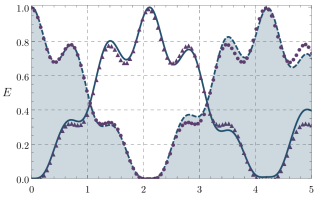
Figure 2: (Color Online) Unitary dynamics of entanglement as a function of dimensionless time $\omega t$. The dashed curve plus shading and the solid line correspond to the exact time evolution of $E_{bc}$ and $E_{ac}$, respectively. Circles and triangles are, respectively, $E_{bc}$ and $E_{ac}$ evaluated within the effective model. The chain consists of $N=10$ oscillators, and the chosen system parameters are $\kappa/\omega=20$, $\alpha=N$, $\beta=1$, $\epsilon/\omega=0.03$, $\Omega/\omega=1$. With this choice, there is resonance with the mode $m=1$, i.e., $\varsigma_{1}=\Omega=\omega$. For the initial state, we choose $r=1$ and $\bar{n}_{c}=0$.

For the parameters used to produce the plots in Fig. 2, the initial entanglement in $[bc]$ is practically fully transferred to the pair $[ac]$. Such highly efficient transfer is observed in Figs. 3 and 4 for steering as well. However, an interesting situation now arises. Although the initial “direct” and “reverse” steerings are equal when $\bar{n}_{c}=0$, see Eq. (IV), their dynamics are interestingly different. In our simulations, the ‘reverse” steering dynamics is closer to entanglement dynamics than the “direct” counterpart. One can see, for instance, that $S_{\overleftarrow{ac}}$ behaves much more like $E_{ac}$ than $S_{\overrightarrow{ac}}$. The same is true for the pair $[bc]$. Furthermore, the “direct” steering $S_{\overrightarrow{bc}}$ suffers sudden death and sudden rebirth (see Fig. 3), while neither the “reverse” steering $S_{\overleftarrow{bc}}$ nor entanglement does so, see Figs. 2 and 4.

Finally, it is interesting to notice that the transfer of “direct” steering shown in Fig. 3 is also abrupt or sudden. The correlation $S_{\overrightarrow{bc}}$ is allowed to arise only after the sudden death of $S_{\overrightarrow{bc}}$. Not only that, there are finite time intervals in which both steerings are null.

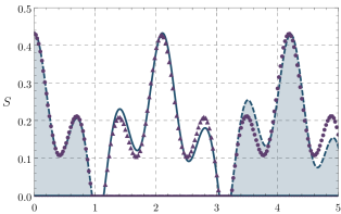
Figure 3: (Color Online) Unitary dynamics of “direct” steering as a function of dimensionless time $\omega t$. The parameters are the same as those in Fig. 2. The dashed curve plus shading and the solid line correspond to the exact time evolution of $S_{\overrightarrow{bc}}$ and $S_{\overrightarrow{ac}}$, respectively. Circles and triangles are, respectively, $S_{\overrightarrow{bc}}$ and $S_{\overrightarrow{ac}}$ evaluated within the effective model.

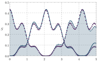
Figure 4: (Color Online) Unitary dynamics of “reverse” steering as a function of dimensionless time $\omega t$. The parameters are the same as those in Fig. 2. The dashed plus shading and the solid line correspond to the exact time evolution of $S_{\overleftarrow{bc}}$ and $S_{\overleftarrow{ac}}$, respectively. Circles and triangles are, respectively, $S_{\overleftarrow{bc}}$ and $S_{\overleftarrow{ac}}$ evaluated within the effective model.

IV.1.2 Initial Mixed States

According to Eq. (IV), we know that an increase in the thermal occupation number $\bar{n}_{c}$ in oscillator $c$ must degrade the total entanglement initially present in the system. This is clearly seen from Fig. 5 by comparing it to Fig. 2. In general, the entanglement dynamics stays qualitatively similar to the unitary case, including the high efficiency. This has been numerically investigated for a broad range of $r$ and $\bar{n}_{c}$. We found that the efficiency of the transport is practically perfect for $0\leq r\leq 5$ and $0\leq\bar{n}_{c}\leq 50$, at the critical point $\omega t_{\star}=2094.4$ [calculated using Eq. (41) with $N=10$, $\alpha=1$, $\beta=10$, and $m=1$]. As mentioned, the critical point is also the maximum of the function $F$ defined in Eq. (LABEL:auxfunc). These numerical results suggest that the maximum value in (42) is exactly equal to $E_{bc}^{t=0}$, but we have not managed to prove it.

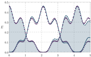
Figure 5: (Color Online) Unitary dynamics of entanglement as a function of dimensionless time $\omega t$. The dashed curve plus shading and the solid line correspond to the exact time evolution of the $E_{bc}$ and $E_{ac}$, respectively. Circles and triangles are, respectively, $E_{bc}$ and $E_{ac}$ evaluated within the effective model. For the initial state, we chose $r=1$ and $\bar{n}_{c}=10$, and the other parameters are the same as in Fig. 2.

On the other hand, the steering presents a richer dynamics due to the possibility of non equivalence between the “direct” and “reverse” cases. This is already manifested in the initial state since, according to Eq. (IV), $S_{\overrightarrow{bc}}^{t=0}=0$ for $r\leq r_{\rm c}={\operatorname{arccosh}}[(3\bar{n}_{c}+1)/(\bar{n}_{c}+1)]$, while $S_{\overleftarrow{bc}}^{t=0}$ is non null. It is remarkable that the “direct” steering is not created dynamically, i.e., $S_{\overrightarrow{ac}}^{t}=0\,\,\,\forall t$, as we could numerically conclude. In other words, there was no “transmutation between species” of steering. In Fig. 6, we show that the “reverse” initial steering, $S_{\overleftarrow{bc}}^{t=0}\neq 0$, is totally transferred to the pair $[ac]$. It is important to report that for values of $r$ greater than the critical value $r_{\rm c}$, the “reverse” steering does not undergo deaths and rebirths similar to Fig. 6, while the “direct” steering (not shown) does.

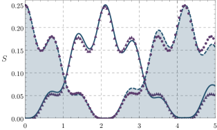
Figure 6: (Color Online) Unitary dynamics of “reverse” steering as a function of dimensionless time $\omega t$. The physical situation is the same as in Fig. 5. The dashed curve plus shading and the solid line correspond to the exact time evolution of $S_{\overleftarrow{bc}}$ and $S_{\overleftarrow{ac}}$, respectively. Circles and triangles are, respectively, $S_{\overleftarrow{bc}}$ and $S_{\overleftarrow{ac}}$ evaluated within the effective model.

From (28) and (IV.1), it is easy to show that the “direct” steering $S_{\overrightarrow{ac}}$ is zero provided

$$F\leq\frac{1}{4}+\frac{{\bar{n}}_{c}}{2({\bar{n}}_{c}+1)(\cosh r-1)}.$$ (44)

The equality is observed when there is sudden death or rebirth of $S_{\overrightarrow{ac}}$. In spite of the fact that the LHS of (44) is a highly transcendental function, it does not depend on the details of the initial state, i.e., $r$ and $\bar{n}_{c}$, and it can, in principle, be numerically solved. For the parameters used in Fig. 3, the use of Eq. (44) allows one to predict that $S_{\overrightarrow{ac}}$ will be non-null in the interval $1143.1\leq\omega t\leq 3045.8$. The condition for the nullity of the “direct steering” $S_{\overrightarrow{bc}}$ can be obtained in a similar way, but it is much more involved since it involves the functions $G$, $H$, and $I$. However, it can be handled, and we applied it to find that $S_{\overrightarrow{bc}}$ will vanish in the interval $951.3\leq\omega t\leq 3237.5$. This is in complete agreement with the plots shown in Fig. 3.

The next natural step is to include thermal excitations in the other oscillators as well. For this, let us consider the CM (13)

$$\!\!{\bf V}^{\prime}_{\!0}\!=\!\hbar(\bar{n}+\tfrac{1}{2})\!\left[\!\left(\!\begin{array}[]{cccc}1&0&0&0\\ 0&s&w&0\\ 0&w&s&0\\ 0&0&0&1\end{array}\!\right)\!\oplus\!\left(\!\begin{array}[]{cccc}1&0&0&0\\ 0&s&-w&0\\ 0&-w&s&0\\ 0&0&0&1\end{array}\!\!\right)\right],$$ (45)

where $s:=\cosh r$, $w:=\sinh r$, $r\geq 0$ is the squeezing parameter, and $\bar{n}\geq 0$ is the mean number of thermal photons of each oscillator. The initial entanglement and steering now read

$$E_{bc}^{t=0} = \max[0,r-{\rm ln}(2\bar{n}+1)],$$

$$S_{\overrightarrow{bc}}^{t=0} = S_{\overleftarrow{bc}}^{t=0}=\max\left[0,{\rm ln}\left(\frac{\cosh r}{2\bar{n}+1}\right)\right],$$ (46)

from which it follows that the state of $b$ and $c$ will be entangled only when marian

$$r>{\rm ln}[(2\bar{n}+1)].$$ (47)

By the same token, that state will be steerable only when $r>\operatorname{arccosh}(2\bar{n}+1)$. Note that ${\bf V}^{\prime}_{\!0}=(2\bar{n}+1){\bf V}_{\!0}|_{\bar{n}_{c}=0}$, with ${\bf V}_{\!0}$ in Eq. (32), such that the application of Eq. (27) results in

$$\!\!\!\!E_{uv}({\bf V}^{\prime}_{\!0})=\max\left[0,E_{uv}({\bf V}_{\!0}|_{\bar{n}_{c}=0})-{\rm ln}(2\bar{n}+1)\right].$$ (48)

From Eq. (28),

$$S_{\overrightarrow{\overleftarrow{uv}}}({\bf V}^{\prime}_{\!0})=\max\left[0,S_{\overrightarrow{\overleftarrow{uv}}}({\bf V}_{\!0}|_{\bar{n}_{c}=0})-{\rm ln}(2\bar{n}+1)\right].$$ (49)

The immediate conclusion is that the presence of the thermal excitations reduces uniformly both the initial entanglement and steering by a factor of ${\rm ln}(2\bar{n}+1)$ when compared to the pure state ${\bf V}_{\!0}|_{\bar{n}_{c}=0}$. The evolution of these two quantities is presented in Figs. 2, 3, and 4. From these, a finite $\bar{n}$ indeed affects the total correlations available to propagate, but the transfer process itself remains very efficient. The explanation relies on the fact that all time dependence is still contained only in the functions $F$ and $I$, which do not depend on $r$ or $\bar{n}$. Given that there are no qualitative differences from the previous simulations, we do not show plots for this case.

IV.2 Interaction with the Environment

To take into account the influence of the environment on the transport of correlations, the dynamics of the CM will now be described by Eq. (17) in the effective model and by Eqs. (1) and (5) in the exact model. The analysis of Eq. (17) reveals that the influence of the initial state, through ${\mathbf{V}}_{0}$, is progressively attenuated with characteristic time $\zeta^{-1}$. In other words, the reservoirs progressively erase the initial correlations in the system. This can be seen from the asymptotic state,

$$\!\!\!\lim_{t\to\infty}\check{\bf V}(t)=\frac{1}{\zeta}\check{\bf D}=\hbar(\bar{n}_{\rm th}+\tfrac{1}{2})\!\left(\!\mathsf{I}_{3}\oplus\frac{\zeta_{m}}{\omega}\oplus\mathsf{I}_{3}\oplus\frac{\omega}{\zeta_{m}}\!\right),$$ (50)

which is completely uncorrelated.

In Figs. 7 and 8, we plot the dynamical behavior of logarithmic negativity and steering, respectively. It is clear that both are progressively destroyed, as predicted by Eq. (50).

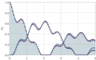
Figure 7: (Color Online) Open system dynamics of entanglement as a function of dimensionless time $\omega t$. The dashed curve plus shading and the solid line correspond to the exact time evolution of $E_{bc}$ and $E_{ac}$, respectively. Circles and triangles are, respectively, $E_{bc}$ and $E_{ac}$ evaluated within the effective model. The parameters are the same as in Fig. 2, except for the new ones that concern interaction with the reservoirs. They are chosen here to be $\bar{n}_{\rm th}=0.1$ and $\zeta/\omega=10^{-4}$.

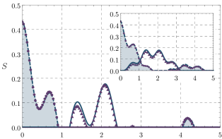
Figure 8: (Color Online) Open system dynamics of “direct” steering as a function of dimensionless time $\omega t$. The parameters are the same as those in Fig. 7. The dashed curve plus shading and the solid line correspond to the exact time evolution of $S_{\overleftarrow{bc}}$ and $S_{\overleftarrow{ac}}$, respectively. Circles and triangles are, respectively, $S_{\overleftarrow{bc}}$ and $S_{\overleftarrow{ac}}$ evaluated within the effective model. Inset: The same for “reverse” steering. The dashed curve plus shading and the solid line correspond to the exact time evolution of $S_{\overrightarrow{bc}}$ and $S_{\overrightarrow{ac}}$, respectively. Circles and triangles are, respectively, $S_{\overrightarrow{bc}}$ and $S_{\overrightarrow{ac}}$ evaluated within the effective model.

V Mutual Information and Quantum Discord

We now analyze the propagation of mutual information and quantum discord initially present in the pair $[bc]$. Let us start once again by considering an initial state in which the pair $[bc]$ is found in a TMTSS, while the remaining oscillators are prepared in a product of local vacuum states. In the sequence, we will consider thermal excitations in all oscillators, and we will also discuss the effect of thermal reservoirs.

For the unitary evolution, and CM given by Eq. (32), we can use the local invariants in Eq. (IV) to calculate the initial amount of mutual information and discord, using Eqs. (23) and (26), respectively. These will be propagated to the pair $[ac]$. The dynamics of these correlations is presented in Fig. 9. It is interesting to see that, just like steering, these correlations have the same critical points and the efficiency of propagation as entanglement, see Fig. 2. Also, in spite of the fact that discord too is asymmetric with respect to the parties, there is no qualitative difference in their behavior like for steering (compare Figs. 3 and 4). Indeed, both kinds of discord behave much like the entanglement with no sudden death or rebirth. Note also that when the mutual information vanishes, the other correlations do as well, while the converse is not true. This corroborates the fact that mutual information contains both classical and quantum correlations.

By heating oscillator $c$, the initial mutual information, unlike entanglement, increases with $\bar{n}_{c}$. This is a result of the dependence on $\bar{n}_{c}$ which is found in Eq. (IV). Interesting enough, while “direct” discord diminished with the increase of $\bar{n}_{c}$, the “reverse” discord did the opposite, compare Figs. 9 and Fig. 10. Consequently, some quantumness is benefited by the increase of $\bar{n}_{c}$. One can also notice from Fig. 10 that the efficiency of transport was not affected by thermal excitations initially present in oscillator $c$.

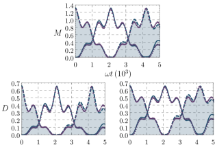
Figure 9: (Color Online) Unitary dynamics of Mutual Information and Quantum Discord as a function of dimensionless time $\omega t$. The parameters are the same as those of Fig. 2. Top: The dashed curve plus shading and the solid line correspond to the exact time evolution of $M_{bc}$ and $M_{ac}$, respectively. Bottom Left: The dashed curve plus shading and the solid line correspond to the exact time evolution of “direct” discords $D_{\overrightarrow{bc}}$ and $D_{\overrightarrow{ac}}$, respectively. Bottom Right: The dashed curve plus shading and the solid line correspond to the exact time evolution of “reverse” discords $D_{\overleftarrow{bc}}$ and $D_{\overleftarrow{ac}}$, respectively. For all plots, circles and triangles are the respective effective models.

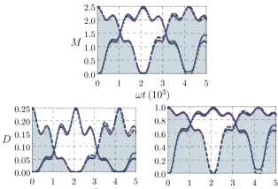
Figure 10: (Color Online) Unitary dynamics of Mutual Information and Quantum Discord as a function of dimensionless time $\omega t$. The physical situation is the same as in Fig. 5. The description of the curves is as in Fig. 9.

Now we consider thermal excitations in all oscillators, just like at the end of Sec. IV.1.2. The effective model uses the initial CM defined in Eq. (45), and we found

$$\mathcal{I}_{b} = \mathcal{I}_{c}=(2\bar{n}+1)^{2}\cosh^{2}r,$$

$$\mathcal{I}_{bc} = -(2\bar{n}+1)^{2}\sinh^{2}r,$$ (51)

which are used to calculate the initial mutual information and discord in the pair $[bc]$. The evolution of these correlations is plotted in Fig. 11, where one can see that the available mutual information and discord (both directions) decreased with $\bar{n}$ (compare to Fig. 9). It is interesting to notice that the initial state is symmetric with respect to discord; that is, at $t=0$ we have $D_{\overrightarrow{bc}}=D_{\overleftarrow{bc}}$. This happens because, for the initial state characterized by Eq. (45), one finds $\mathcal{I}_{b}=\mathcal{I}_{c}$. However, as time passes, this symmetry is dynamically lost. For the regime considered here and in spite of the presence of thermal excitations, the high efficiency of the propagation of mutual information and discord is preserved, just like what happened to entanglement and steering.

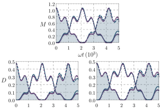
Figure 11: (Color Online) Unitary dynamics of Mutual Information and Quantum Discord as a function of dimensionless time $\omega t$. The description of the curves is as in Fig. 9, and the frequencies and coupling constants are the same as in Fig. 2. All oscillators start in local thermal states with mean occupation number $\bar{n}=10$, except for the pair $[bc]$, which is in a TMTSS with $r=1$ and the same number of thermal excitations as the other oscillators. The initial state for the effective model has the CM in Eq. (45) with $r=1$ and $\bar{n}=10$.

If we let the chain interact with environmental thermal baths, the time evolution of the CM is given by Eq. (17). Basically, our simulations (not shown) indicated that mutual information and discord behaved very much like the entanglement, as already shown in Fig. 7. To be more specific, they dynamically decrease with a time scale of $\zeta^{-1}$ until completely vanishing in the asymptotic limit, see Eq. (50). For this reason, we chose not to show plots for this case.

In all situations analyzed so far, the propagation of correlations took place in a scenario where entanglement was always present. However, it is possible to consider initial states in which there is no entanglement but there are other forms of quantum or classical correlations present. We are interested in exploring this problem now, i.e., we want to investigate propagation of these other-than-entanglement correlations in a situation with no entanglement. For this aim, we consider the initial state with the CM given by Eq. (45), with the choice $r<{\rm ln}[(2\bar{n}+1)]$, see Eq. (47). As one can see in Fig. 12, transport is still equally efficient, even in the absence of entanglement.

Figure 12: (Color Online) Unitary dynamics of Mutual Information and Quantum Discord as a function of dimensionless time $\omega t$. The physical situation is the same as in Fig. 11, except for the initial state of the pair $[bc]$, which is now separable. The initial CM used in the effective model is given by Eq. (45) with $r=1/2$ and $\bar{n}=10$.

VI Propagation of Bell Correlations

We now focus on the propagation of Bell-like correlations. As previously discussed, they are related to the idea of violation of local realism. To be more specific, we employ Eq. (31) as a quantifier of this type of correlation. At this point, one must have in mind that no violation of one form of the Bell inequality does not necessarily exclude violation of local realism in other configurations, i.e., other inequalities built with results from different measurements. For the purposes of this paper, it is enough to investigate propagation of only one type of Bell-like correlation, which is the one quantified by Eq. (31).

We consider the case of unitary evolution (already discussed) and two initial preparations. In one case, the state is pure, and in the other there are thermal excitations in oscillator $c$ (mixed state). These preparations have also been previously considered, e.g., in Figs. 2 and 5, respectively. The dynamics is shown in Fig. 13. Note that violation for the pair $[ac]$ is attained around $\omega t=2\times 10^{3}$ for the pure-state case (left panel). Just like before, this kind of correlation is also efficiently transmitted through the chain. It is worthwhile to notice that, during the violation, the state is both entangled and steerable, see Figs. 2, 3 and 4. This is expected from the well-known hierarchy discussed earlier and presented in jones . By increasing the thermal energy in oscillator $c$, it comes to a point at which the correlations are not enough to violate local realism. This is shown in the right panel of Fig. 13. It is interesting to see that the setup still works efficiently to propagate the correlations.

The interaction with thermal baths does not bring much new physics for the propagation of this kind of correlation. As before, it is progressively destroyed on a time scale $\zeta^{-1}$. This destructive effect is expected, giving the fact that $\bar{B}_{uv}$ depends on Wigner functions, whose deleterious impact, as consequence of the action of thermal baths, is well known.

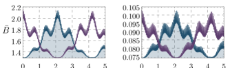
Figure 13: (Color Online) Unitary dynamics of Bell correlations as a function of dimensionless time $\omega t$. The curve without shading is the exact time evolution of $\bar{B}_{ac}$, while the curve with the shading is the exact time evolution of the $\bar{B}_{bc}$. We avoided the comparison with the effective model due to the presence of very small oscillations, which makes visualization problematic. Left: Unitary pure-state evolution as in Fig. 2. Right: Unitary mixed-state evolution as in Fig. 5.

Final Remarks

We provided a detailed study of the problem of propagation of correlations through a system of coupled harmonic oscillators. We considered propagation in the closed system scenario as well as in the presence of heat reservoirs. In addition, we studied the effect of having initially pure or mixed entangled states or even non entangled mixed states with non-null discord. The presence of thermal excitations in the system was also investigated. We chose a particular configuration to this study which is well known to be reducible to a three-body system. This allowed us to provide analytical results that were useful for understanding the rich behavior found in the propagation of different correlations. We could, for instance, spot fundamental differences in the dynamical behavior of steering and discord, which are quantities that can be defined in non equivalent ways in the same bipartite system.

It is important to remark that we performed simulations for a variety of chain lengths $N$ (smaller or bigger than the one considered here) and the same qualitative behavior was found. Of course, $N$ cannot be deliberately increased since this brings the chain spectrum to a continuum what spoils the transfer considerably. This was previously shown in the context of entanglement in plenio2005 . To the best of our knowledge, this is the first work to bring together entanglement, steering, mutual information, discord, and Bell-type correlations to a comparative study from the important point of view of quantum transport. We hope this work can motivate further investigation in other setups, such as the ones found in coupled quantum electrodynamic systems, in which two-level systems can couple with harmonic oscillators, forming polarons. Another possibility is to use more intricate topologies of coupled systems using the general simplification approach presented in nicacio4 . It would be interesting to study the propagation of discord and steering in these different scenarios to see whether or not the asymmetry, present in the definition of these correlations, can also be pinpointed in those physical systems.

Appendix

The symplectic matrix $\mathsf{E}_{t}$ in (17) is written as

$${\mathsf{E}}_{t}=\left(\begin{array}[]{rl}\mathbf{C}&\mathbf{S}\\ -\mathbf{S}&\mathbf{C}\end{array}\right),$$ (A-1)

with the matrices $\mathbf{C}:=\cos({\bf H}t)$ and $\mathbf{S}:=\sin({\bf H}t)$ for ${\bf H}$ in Eq. (16). Explicitly, their elements are

$${\mathbf{C}}_{11} = \frac{\omega}{\varsigma_{m}}\frac{\boldsymbol{O}_{\!m\alpha}^{2}[(\chi-1)\,+\,\cos(\chi\tau)]\,+\,\chi\,\boldsymbol{O}_{\!m\beta}^{2}\cos\tau}{(\chi-1)\chi},$$

$${\mathbf{C}}_{12} = \frac{\omega}{\varsigma_{m}}\frac{\boldsymbol{O}_{\!m\alpha}\boldsymbol{O}_{\!m\beta}[(\chi-1)\,-\,\chi\cos\tau\,+\,\cos(\chi\tau)]}{(\chi-1)\chi},$$

$${\mathbf{C}}_{21} = {\mathbf{C}}_{12},$$

$${\mathbf{C}}_{14} = 2\sqrt{\frac{\omega}{\varsigma_{m}}}\frac{{\boldsymbol{O}}_{m\alpha}}{\chi}\sin^{2}\left(\frac{\chi\tau}{2}\right),$$

$${\mathbf{C}}_{22} = \frac{\omega}{\varsigma_{m}}\frac{\chi\,\boldsymbol{O}_{\!m\alpha}^{2}\cos\tau\,+\,\boldsymbol{O}_{\!m\beta}^{2}[(\chi-1)\,+\,\cos(\chi\tau)]}{(\chi-1)\chi},$$

$${\mathbf{C}}_{24} = {\mathbf{C}}_{42}=2\sqrt{\frac{\omega}{\varsigma_{m}}}\frac{\boldsymbol{O}_{\!m\beta}}{\chi}\sin^{2}\left(\frac{\chi\tau}{2}\right),$$

$${\mathbf{C}}_{13} = {\mathbf{C}}_{31}={\mathbf{C}}_{23}={\mathbf{C}}_{32}={\mathbf{C}}_{34}={\mathbf{C}}_{43}=0,$$

$${\mathbf{C}}_{33} = 1,$$

$${\mathbf{C}}_{44} = \frac{1+(\chi-1)\cos(\chi\tau)}{\chi}$$ (A-2)

and

$${\mathbf{S}}_{11} = \frac{\omega}{\varsigma_{m}}\frac{\boldsymbol{O}_{\!m\alpha}^{2}\sin(\chi\tau)\,+\,\chi\boldsymbol{O}_{\!m\beta}^{2}\sin\tau}{(\chi-1)\chi},$$

$${\mathbf{S}}_{12} = {\mathbf{S}}_{21}=\frac{\omega}{\varsigma_{m}}\frac{\boldsymbol{O}_{\!m\alpha}\boldsymbol{O}_{\!m\beta}[\sin(\chi\tau)-\chi\sin\tau]}{(\chi-1)\chi},$$

$${\mathbf{S}}_{13} = {\mathbf{S}}_{31}={\mathbf{S}}_{23}={\mathbf{S}}_{32}={\mathbf{S}}_{33}={\mathbf{S}}_{34}={\mathbf{S}}_{43}=0,$$

$${\mathbf{S}}_{14} = {\mathbf{S}}_{41}=-\sqrt{\frac{\omega}{\varsigma_{m}}}\frac{\boldsymbol{O}_{\!m\alpha}}{\chi}\sin(\chi\tau),$$

$${\mathbf{S}}_{22} = \frac{\omega}{\varsigma_{m}}\frac{\boldsymbol{O}_{\!m\alpha}^{2}\chi\sin\tau\,+\,\boldsymbol{O}_{\!m\beta}^{2}\sin(\chi\tau)}{(\chi-1)\chi},$$

$${\mathbf{S}}_{24} = {\mathbf{S}}_{42}=-\sqrt{\frac{\omega}{\varsigma_{m}}}\frac{\boldsymbol{O}_{\!m\beta}}{\chi}\sin(\chi\tau),$$

$${\mathbf{S}}_{44} = \frac{\chi-1}{\chi}\sin(\chi\tau),$$ (A-3)

where we have defined

$$\tau:=\epsilon t/4,\,\,\,\chi:=\frac{\omega}{\varsigma_{m}}\boldsymbol{O}_{\!m\alpha}^{2}+\frac{\omega}{\varsigma_{m}}\boldsymbol{O}_{\!m\beta}^{2}+1.$$ (A-4)

The functions appearing in Eqs. (IV.1) and (IV.1) are

$$F := \frac{\omega^{2}}{\varsigma_{m}^{2}}\frac{\boldsymbol{O}_{\!m\alpha}^{2}{\boldsymbol{O}}_{m\beta}^{2}}{\chi(\chi-1)}\left[\tfrac{\chi-\cos[(\chi-1)\tau]}{(\chi-1)}+\tfrac{\cos(\chi\tau)-1}{\chi}-{\cos\tau}\right],$$

$$G := \frac{\omega^{2}}{\varsigma_{m}^{2}}\frac{\boldsymbol{O}_{m\alpha}^{4}}{(\chi-1)^{2}}+\frac{\omega^{2}}{\varsigma_{m}^{2}}\frac{\boldsymbol{O}_{m\beta}^{4}(\chi^{2}-2\chi+2)}{\chi^{2}(\chi-1)^{2}},$$

$$H := \frac{\omega}{\varsigma_{m}}\frac{\boldsymbol{O}_{m\beta}^{2}}{\chi^{2}}+\frac{\omega^{2}}{\varsigma_{m}^{2}}\frac{\boldsymbol{O}_{m\alpha}^{2}\boldsymbol{O}_{m\beta}^{2}(\chi^{2}-\chi+1)}{\chi^{2}(\chi-1)^{2}},$$

$$I := \frac{\omega^{2}}{\varsigma_{m}^{2}}\frac{{\boldsymbol{O}}_{m\alpha}^{2}{\boldsymbol{O}}_{m\beta}^{2}}{\chi(\chi-1)}\!\left[\tfrac{\cos[(\chi-1)\tau]}{(\chi-1)}+\frac{{\boldsymbol{O}}_{m\beta}^{2}}{{\boldsymbol{O}}_{m\alpha}^{2}}\tfrac{\cos[\chi\tau]}{\chi}+{\cos\tau}\right].$$

References

- (1) R. Horodecki, P. Horodecki, M. Horodecki & K. Horodecki, Quantum entanglement, Rev. Mod. Phys. 81, 865 (2009), arXiv:quant-ph/0702225v2.
- (2) N. Gisin, Bell’s inequality holds for all non-product states, Phys. Lett. A 154, 201 (1991).
- (3) S.J. Jones, H.M. Wiseman & A.C. Doherty, Entanglement, Einstein - Podolsky - Rosen correlations, Bell nonlocality, and Steering, Phys. Rev. A 76, 052116 (2007), arXiv:quant-ph/0709.0390v2.
- (4) H.M. Wiseman, S.J. Jones & A.C. Doherty, Steering, Entanglement, Nonlocality, and the Einstein - Podolsky - Rosen Paradox, Phys. Rev. Lett. 98, 140402 (2007), arXiv:quant-ph/0612147v3.
- (5) H. Ollivier & W.H. Zurek, Quantum Discord: A Measure of the Quantumness of Correlations, Phys. Rev. Lett. 88, 017901 (2001), arXiv:quant-ph/0105072v3.
- (6) L. Henderson & V. Vedral, Classical, quantum and total correlations, J. Phys. A 34, 6899 (2001), arXiv:quant-ph/0105028v1.
- (7) B. Groisman, S. Popescu & A. Winter, Quantum, classical, and total amount of correlations in a quantum state, Phys. Rev. A 72, 032317 (2005), arXiv:quant-ph/0410091.
- (8) L. Amico, R. Fazio, A. Osterloh & V. Vedral, Entanglement in many-body systems, Rev.Mod.Phys. 80, 517 (2008), arXiv:quant-ph/0703044v3.
- (9) M.B. Plenio, J. Hartley & J. Eisert, Dynamics and manipulation of entanglement in coupled harmonic systems with many degrees of freedom, New J. Phys. 6, 36 (2004), arXiv:quant-ph/0402004v2.
- (10) M. Plenio & F.L. Semião, High efficiency transfer of quantum information and multiparticle entanglement generation in translation-invariant quantum chains, New J. Phys. 7, 73 (2005), arXiv:quant-ph/0407034v2.
- (11) F. Nicacio & F.L. Semião, Coupled Harmonic Systems as Quantum Buses in Thermal Environments, arXiv:quant-ph/ 1601.07528v1.
- (12) E. Buks & M.L. Roukes, Electrically tunable collective response in a coupled micromechanical array, J. Microelectromech. Syst. 11, 802 (2002).
- (13) A. Bermudez, T. Schaetz & D. Porras, Synthetic Gauge Fields for Vibrational Excitations of Trapped Ions, Phys. Rev. Lett 107,150501 (2011), arXiv:quant-ph/1104.4734v2.
- (14) F. Nicacio, R.N.P. Maia, F. Toscano & R.O. Vallejos, Phase space structure of generalized Gaussian cat states, Phys. Lett. A 374, 4385 (2010), arXiv:quant-ph/1002.2248v1 [quant-ph].
- (15) R.F. Werner, Quantum states with Einstein-Podolsky-Rosen correlations admitting a hidden-variable model, Phys. Rev. A 40, 4277 (1989).
- (16) P.P. Munhoz, J.A. Roversi, A. Vidiella-Barranco & F.L. Semião, Spontaneous emission and teleportation in cavity QED, J. Phys. B: At. Mol. Opt. Phys. 38, 3875 (2005), arXiv:quant-ph/0504159.
- (17) C.H. Bennett, D.P. DiVincenzo, J.A. Smolin & W.K. Wootters, Mixed-state entanglement and quantum error correction, Phys. Rev. A 54, 3824 (1996), arXiv:quant-ph/9604024.
- (18) A. Grossmann, Parity operator and quantization of -functions, Comm. Math. Phys. 48, 191 (1976), Project Euclid 1103899886.
- (19) A. Royer, Wigner functions as the expectation value of a parity operator, Phys. Rev. A 15, 449 (1977).
- (20) A.M. Ozorio de Almeida, The Weyl representation in classical and quantum mechanics, Phys. Rep. 295, 265 (1998).
- (21) R. Simon, Peres-Horodecki Separability Criterion for Continuous Variable Systems, Phys. Rev. Lett. 84, 2726 (2000), arXiv:quant-ph/9909044v1.
- (22) A. Serafini, F. Illuminati, and S.D. Siena, Symplectic invariants, entropic measures and correlations of Gaussian states, J. Phys. B 37, L21 (2004), arXiv:quant-ph/0307073v4.
- (23) A. Datta, A. Shaji & C.M. Caves, Quantum discord and the power of one qubit, Phys. Rev. Lett. 100, 050502 (2008), arXiv:quant-ph/0709.0548v1.
- (24) E. Knill & R. Laflamme, Power of One Bit of Quantum Information, Phys. Rev. Lett. 81, 5672 (1998), arXiv:quant-ph/9802037v1.
- (25) T.K. Chuan, J. Maillard, K. Modi, T. Paterek, M. Paternostro & M. Piani, Quantum discord bounds the amount of distributed entanglement, Phys. Rev. Lett. 109, 070501 (2012), arXiv:1203.1268v3.
- (26) P. Giorda & M.G.A. Paris, Gaussian quantum discord, Phys. Rev. Lett. 105, 020503 (2010), arXiv:1003.3207v2[quant-ph].
- (27) S. Pirandola, G. Spedalieri, S.L. Braunstein, N.J. Cerf & S. Lloyd, Optimality of Gaussian Discord, Phys. Rev. Lett. 113, 140405 (2014), arXiv:quant-ph/1309.2215v3 .
- (28) C. Branciard, E.G. Cavalcanti, S.P. Walborn, V. Scarani & H.M. Wiseman, One-sided Device-Independent Quantum Key Distribution: Security, feasibility, and the connection with steering, Phys. Rev. A 85, 010301(R) (2012), arXiv:1109.1435v3.
- (29) I. Kogias, A.R. Lee, S. Ragy & G. Adesso, Quantification of Gaussian quantum steering, Phys. Rev. Lett. 114, 060403 (2015), arXiv:quant-ph/1410.1637v3.
- (30) K. Banaszek & K. Wódkiewicz, Testing Quantum Nonlocality in Phase Space, Phys. Rev. Lett. 82, 2009 (1999), arXiv:quant-ph/9806068; K. Wódkiewicz, Nonlocality of the Schrödinger cat, N. J. Phys. 2, 21 (2000); A.M. Ozorio de Almeida & O. Brodier, Parity Measurements, Decoherence and Spiky Wigner Functions, J. Phys. A: Math. Gen. 37 L249, (2004), arXiv:quant-ph/0312098.
- (31) P. Marian, T.A. Marian & H. Scutaru, Bures distance as a measure of entanglement for two-mode squeezed thermal states, Phys. Rev. A 68, 062309 (2003).