The evolution in the stellar mass of Brightest Cluster Galaxies over the past 10 billion years

Abstract

Using a sample of 98 galaxy clusters recently imaged in the near infra-red with the ESO NTT, WIYN and WHT telescopes, supplemented with 33 clusters from the ESO archive, we measure how the stellar mass of the most massive galaxies in the universe, namely Brightest Cluster Galaxies (BCG), increases with time. Most of the BCGs in this new sample lie in the redshift range $0.2<z<0.6$, which has been noted in recent works to mark an epoch over which the growth in the stellar mass of BCGs stalls. From this sample of 132 clusters, we create a subsample of 102 systems that includes only those clusters that have estimates of the cluster mass. We combine the BCGs in this subsample with BCGs from the literature, and find that the growth in stellar mass of BCGs from 10 billion years ago to the present epoch is broadly consistent with recent semi-analytic and semi-empirical models. As in other recent studies, tentative evidence indicates that the stellar mass growth rate of BCGs may be slowing in the past 3.5 billion years. Further work in collecting larger samples, and in better comparing observations with theory using mock images is required if a more detailed comparison between the models and the data is to be made.

1 Introduction

Brightest Cluster Galaxies (BCGs) are the brightest and most massive galaxies in the universe. They form within galaxy clusters, and generally lie near the bottom of the cluster gravitational potential well. They have unique properties, including extended light profiles, and they are brighter than the cluster luminosity function leads us to expect (Loh & Strauss, 2006; von der Linden et al., 2007; Shen et al., 2013). These properties differentiate them from other elliptical galaxies.

Most BCGs can be readily identified in observations as a result of their brightness and dominance within a galaxy cluster. Additionally, N-body simulations can be carried out to create mock galaxy clusters, which also contain readily-identifiable BCGs. These observed and simulated BCGs can be directly compared, and this allows us to test models that describe the growth of these BCGs - a task that is difficult to do with galaxies in general as a result of the large variety of different types of galaxies, with varying formation histories.

Initially, there was considerable disagreement between the models and the observations, with models predicting a factor of three increase in the stellar mass of BCGs between $z=1$ and today (De Lucia & Blaizot, 2007, hereafter referred to as DLB07), and observations showing little growth over the same redshift interval (see Stott et al., 2010, for example). While more recent models (Tonini et al., 2012; Shankar et al., 2014, 2015) and observations (Lin et al., 2013; Lidman et al., 2012) are now in better agreement with one another with both predicting or showing a doubling of the stellar mass since $z\sim 1$, there is still some disagreement as to when this growth occurs. In the semi-empirical model of Shankar et al. (2015), the stellar mass of BCGs continues to increase to the present day. However, in the semi-analytic model of Tonini et al. (2012), the growth appears to stall after $z\sim 0.4$. There is some observational support for the second model. Lin et al. (2013) find that most of of the growth since $z\sim 1.5$ occurs in the redshift range $0.5<z<1.5$. Similarly, Oliva-Altamirano et al. (2014) find no significant growth in the range $0.09<z<0.27$, and Inagaki et al. (2014), who explores the redshifts range $0.2<z<0.4$, find an increase of between 2 and 14%. In contrast to these results, Bai et al. (2014) find an increase of 50% between $z=0.5$ and $z=0.1$, and Zhang et al. (2015) find an increase of 35% between $z=1$ and the present day.

The aim of this study is to make a more detailed measurement of the growth of BCGs using new data that covers the redshift interval over which the growth appears to stall. The paper is outlined as follows. §2 describes the data used and the steps used to process them, and §3 outlines how the stellar masses of the BCGs and clusters within the sample were determined. The analysis of the data is carried out in §4, and the discussion and conclusions are presented in §5 and §6 respectively. Throughout this paper we use Vega magnitudes, and assume a $\Lambda$CDM cosmology with $\Omega_{M}=0.3$, $\Omega_{\Lambda}=0.7$ and $H_{0}=70\text{\ km\ s}^{-1}\text{\ Mpc}^{-1}$.

2 Data

We utilise a sample of 98 newly imaged galaxy clusters from the RELICS survey within this study. The data were collected during 6 observing runs on three instruments over a period spanning from October 2013 to March 2015. The instruments utilised were the SofI camera on the New Technology Telescope at the ESO La Silla Observatory in Chile (Moorwood, Cudy & Lidman, 1998), WHIRC on the WIYN telescope at the Kitt Peak National Observatory (Miexner et al., 2010) and LIRIS on the William Herschel Telescope in La Palma, Spain. The observing runs are summarised in Table 1.

Table 1: Observing runs

Instrument	Telescope	Dates
WHIRC	WIYN	2013 October 11-14
LIRIS	WHT	2014 December 12-14
SofI	NTT	2014 January 18-21
LIRIS	WHT	2014 October 3-4
SofI	NTT	2014 December 5-8
LIRIS	WHT	2015 March 6-8

RELICS uses massive clusters from the SPT (Carlstrom et al., 2011), ACT (Swetz et al., 2011), MACS (Ebeling, Edge & Henry, 2001) and C1G (Buddendiek et al., 2015) cluster catalogues as gravitational telescopes to search for lensed compact early-type galaxies (also know as red nuggets). Many of the clusters within the RELICS survey are drawn from the “Weighting the Giants” Survey (von der Linden et al., 2014), which has provided deep Subaru imaging of a selection of MACS clusters, in addition to a sample of Abell clusters. Clusters in the MACS sample (Ebeling et al., 2010) are X-ray selected, whereas the clusters in the SPT/ACT samples (Staniszewski et al., 2009; Williamson et al., 2011; Marriage et al., 2011; Hasselfield et al., 2013) have been discovered through the Sunyaev-Zel’Dovich effect. Clusters in the C1G cluster catalogue were selected from a joint search of ROSAT all sky survey and data-release 8 of the Sloan Digital Sky Survey. RELICS clusters are massive, and have a median mass of $10^{15}M_{\odot}$.

This sample was then augmented by carrying out a search of the ESO archives of the SofI instrument. These data were obtained from September 1998 to February 2012, and this search resulted in an additional 31 clusters being added to the sample.

The clusters are all imaged in the Ks-band, with typical exposure times of $\sim 2700$s, which result in 5-$\sigma$ depths of 19.5 mag. These observations are all deeper than what is necessary for the analysis of BCGs, as they were designed to detect background galaxies gravitationally lensed by the cluster. At the redshift range of the sample, BCGs have Ks-band magnitudes of 12-17 mag, and therefore each BCG is detected with a minimum signal-to-noise ratio of 50.

Table 2: Observational summary
(see https://github.com/SabineBellstedt/Bellstedt2016—Table-2-Observational-Summary for full table)
Redshift Sources:
(1) Mantz et al. (2010) (2) Mann & Ebeling (2012) (3) Menanteau et al. (2013) (4) Kristian, Sandage & Westphal (1978) (5) Gioia et al. (1998) (6) Ebeling et al. (2007) (7) Abell, Corwin & Olowin (1989) (8) SDSS, DR8 (9) Menanteau et al. (2010) (10) Werner et al. (2007) (11) Jones et al. (2009) (12) NASA Astrophysical Database (13) van Weeren et al. (2012) (14) Williamson et al. (2011) (15) Story et al. (2011) (16) Aganim et al. (2012) (17) Sifón et al. (2013) (18) Ebeling et al. (2010) (19) Applegate et al. (2014) (20) Ruel et al. (2014) (21) Buddendiek et al. (2015) (22) Wen & Han (2013) (23) Piffaretti et al. et al. (2011) (24) Vanderlinde et al. (2010) (25) von der Linden et al. (2014) (26) Sifón et al. (2013) (27) Brodwin et al. (2010)

Cluster	RA	Dec	$z_{spec}$	$z_{phot}$	z Source	Instrument/Telescope	Exposure Time
	J2000	J2000					[s]
SPT-CL-J0000-5748	00:01:00.04	-57:48:20.7	0.702	…	(20)	NTT/SofI	2700
MACS-J0011.7-1523	00:11:42.80	-15:23:18.34	0.379	…	(18)	WHT/LIRIS	2700
MACS-J0014.3-3022	00:14:15.82	-30:22:14.4	0.308	…	(1)	SofI/NTT	12000
MACS-J0014.3-3022	00:14:17.26	-30:22:34.8	0.308	…	(1)	SofI/NTT	12000
ACT-CL-J0014.9-0057	00:14:54.00	+00:57:10.1	0.533	…	(7)	NTT/SofI	2700

Table 3: Instrument summary

Instrument	Telescope	Pixel Scale	FoV	Detector
		[”]	[’]
SofI	NTT	0.288	4.9	$1024\times 1024$ Rockwell Hawaii HgCdTe
WHIRC	WIYN	0.099	3.7	$2048\times 2048$ Raytheon Virgo HgCdTe
LIRIS	WHT	0.251	4.3	$1024\times 1204$ Hawaii HgCdTe

2.1 Data Reduction

The procedures used in the reduction of the data are standard, and largely follow the steps as outlined by Lidman et al. (2008). Briefly, the pedestal in the images was removed using dark frames, pixels were normalised using dome flats and the sky was removed using a moving median stack of the science data, using our own python scripts and tasks in IRAF.

Zero points were determined by using stars from the 2MASS point source catalogue (Skrutskie et al., 2006). Typically, between 4 and 30 stars were present in each image, and only unsaturated stars with high quality measurements were selected to measure the zero point.

For data taken with LIRIS, we first had to unscramble the image pixels in the FITS header. There was also a residual shade pattern in the sky subtracted images. This was removed by subtracting the median of the data along detector rows. A similar technique was used to remove the crosstalk from bright stars in SofI images.

2.2 Data Analysis

To estimate the magnitudes of galaxies in each cluster, we run SExtractor (Bertin & Arnouts, 1996) on each image, and use MAG_AUTO as a measure of the magnitude. MAG_AUTO is a Kron-like magnitude (Kron, 1980) with an elliptical aperture.

Since the galaxy clusters within the sample were selected to be massive, most of the clusters have a large BCG. The BCG in each cluster was identified visually as the largest, brightest galaxy in the cluster. BCGs are typically in the centre with extended galaxy haloes, unlike their surrounding galaxies. We verified the visual BCG selection by ensuring that these were the galaxies which were indeed the brightest as measured by MAG_AUTO. In some clusters, there appear to be two BCGs of comparable brightness, such as the cluster MACS J0014.3-3022. In such cases, both BCGs were included in the sample.

There are a small number of cases in which the BCGs were not clearly identifiable, usually because of foreground contamination, these clusters are excluded from analysis. The excluded clusters are Abell 521, ACT-CL J0018.2-0022, ACT-CL J0228.5+0030, ACT-CL J0301.1-0110, ACT-CL J0250.1+0008, MACS J2243.3-0935, RX J1132+00 and SPT-CL J0615-5746.

2.3 Additional Samples

To augment the sample used throughout this paper, we include the sample used by Lidman et al. (2012, hereafter L12). This sample includes 103 BCGs presented by Stott et al. (2008) over the redshift range $0.04\leq z\leq 0.83$, 20 BCGs by Stott et al. (2010) over the higher redshift range of $0.81\leq z\leq 1.46$ and 5 BCGs from Collins et al. (2009) over the redshift range $1.22\leq z\leq 1.46$. The study by L12 produced two new BCG samples referred to as the CNOC1 (Yee, Ellingson & Carlberg, 1996) and SpARCS samples. The SpARCS sample includes 12 BCGs spanning the redshift interval $0.867\leq z\leq 1.630$, and the CNOC1 sample has 15 BCGs over the lower redshift range $0.193\leq z\leq 0.547$.

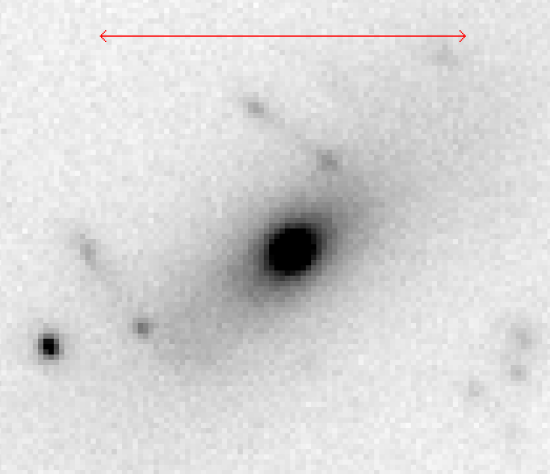
Figure 1: A SofI image in the Ks band of the BCG in the cluster Abell 1553. North is pointing up and east to the left, and the arrow has a length of 20”, which at the cluster redshift of $z=0.165$ corresponds to a distance of 57 kpc. The extended light profile of this BCG is clearly seen in many of the BCGs in our sample. Of particular note in this BCG are the lens-like features offset from the centre of the BCG.

The photometric errors determined by SExtractor tend to underestimate the true error as correlated signal in the pixels is not taken into account. Some of the clusters imaged in the new set of data had previously been analysed by L12. These clusters are; Abell 1204, Abell 1553, Abell 1835, Abell 2390, Abell 68, MACS J0025.4-1222 and MACS J0454.10-0300. We use these clusters to provide a more reliable measure of the errors. The median of the absolute difference in Ks-band magnitude of the BCGs in these images is 0.22 mag, which we have used as the magnitude error of the BCGs in our sample.

2.4 Systematic drifts in the photometry

Throughout this paper we use MAG_AUTO from SExtractor to estimate magnitudes, which are then used to derive masses. In essence, it is an aperture magnitude, so by definition, it does not measure the total magnitude of a galaxy. The amount of flux missed depends on the intrinsic light profile of the galaxy and the seeing. On simulated galaxies, L12 finds that MAG_AUTO misses between 18% and 35% of the flux. Our results are not affected if the amount of flux missed is independent of redshift. However, this assumption may not be true, as the profile of BCGs and therefore the amount of flux lost may change with redshift.

Table 4: Testing the difference between photometric magnitudes produced by MAG_AUTO and GALFIT to eliminate the presence of a measurement bias.

Redshift	Number of	MAG_AUTO -	Scatter
range	clusters	GALFIT
0.00-0.25	10	0.52	0.37
0.25-0.40	5	0.44	0.17
0.40-0.80	10	0.57	0.33
0.00-0.80	25	0.54	0.33

In order to see if this is a large effect, we tried an alternative approach in computing the magnitude of the BCGs in our sample. Following L12, we ran version 3.0.4 of GALFIT on a subsample of BCGs. For this test, we used the BCGs that were observed with SofI and we split the BCGs into three redshift bins. The bin boundaries are the same as those used later in the analysis, i.e. $0<z<0.25$, $0.25<z<0.4$, and $0.4<z<0.8$. We then compared GALFIT magnitudes with MAG_AUTO. The difference between the two is large, with the GALFIT value being on average 0.54 mag brighter than the MAG_AUTO magnitude with a scatter of 0.33 mag when using all 25 BGCs. This is very similar to the difference reported in L12, although our sample is a factor of three larger. When split into the three redshift bins, there is no significant change in the average difference between the three redshift bins.

While this test is not definitive (as any systematic drift may affect MAG_AUTO and GALFIT equally), it is suggestive that the deviations from the models identified in Section 4.2 do not result from systematic uncertainties in the photometry.

3 Determining Stellar Masses

3.1 BCG Stellar Masses

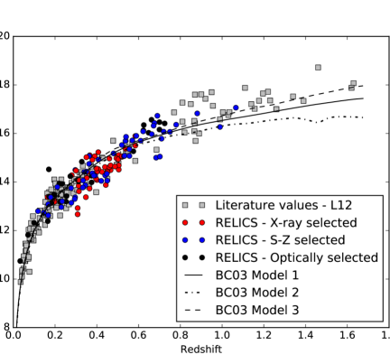
Figure 2: The observer-frame Ks-band magnitude of BCGs as a function of redshift. The data from this paper have been colour coded based on the selection method of the host cluster: X-ray selected clusters have been coloured in red, Sunyaev-Zel’dovich effect selected clusters have been coloured in blue, and the rest have been coloured in black. The stellar population model indicated as BC03 Model 1 is that from Lidman et al. (2012), with $z_{f}=5$, $\tau=0.9$ and a metallicity split 60/40 between solar and 2.5 times solar, as outlined in the text. Other BC03 single burst models are indicated on the plot: BC03 Model 2 has $z_{f}=2$, and BC03 Model 3 has $z_{f}=5$. These models have been normalised so that they agree with the low redshift sample. Note how most of the BCGs above $z\sim 1$ lie above the model.

The stellar masses of BCGs were determined using the method developed in L12, in which the observed Ks-band magnitude is converted into a mass using stellar population synthesis models. In choosing the model, L12 used the J-Ks colour of BCGs over the redshift range $0<z<1.5$ as a constraint. From their comparison, it was determined that the best-fitting stellar population model was a Bruzual & Charlot (2003) model with a Chabrier IMF (Chabrier, 2003), a formation redshift of $z_{f}=5$, a star formation rate e-folding time of 0.9 Gyr and a composite metallically that is split 60/40 between solar and a metallicity that is two and half times solar. Since a large portion of the sample of this paper is in common with the sample of L12, we use this model in our analysis. In converting from luminosity to mass, we assume that the mass-to-light ratios of the BCGs are independent of stellar mass.

Since $\sim 6\%$ of the clusters within the sample do not yet have spectroscopic redshifts, the corresponding masses for the BCGs could not be calculated. Therefore, these clusters were not considered further in this paper.

The observed Ks-band magnitudes of the full sample are plotted against redshift in Figure 2. The new sample of this study is shown as red, blue and black circles, and can be seen to augment the previously sparsely populated region of the plot in the redshift range $0.4<z<0.8$.

In addition to the model described above, we plot two other models to display the effect of modifying the model. Both models, labelled as Model 2 and Model 3 in Figure 2 are single burst models. Model 2 has a formation redshift of $z=2$ and has solar metallicity. Model 3 has a formation redshifts of $z=5$ and has metallicity that is two and half times solar. Since neither model is capable of describing the observed J-Ks colour (see Figure 2 in L12), we do not consider these models further in this paper.

There are some preliminary observations that can be made from Figure 2. The main one is that the BCGs at $z>0.8$ (made up of the samples by Stott et al. (2010), Collins et al. (2009) and the SpARCS sample) tend to lie above the stellar population model. Within the redshift interval $0.6<z<0.8$, this trend ends. For the new sample of this paper, the opposite effect is noticed. While the effect is not so strong as for the high-z BCGs, the new BCGs are more likely to fall below the model than above, indicating that they are more massive than the model suggests. What is important to note however, is that larger clusters tend to host larger BCGs, and therefore it is not possible to make judgements about the growth of BGCs without accounting for their corresponding cluster masses. This is discussed further in the next section. Another observation to be noted is that X-ray selected clusters tend to host brighter BCGs. As will become clear in the next section, this occurs because the X-ray selected clusters in our sample are, on average, more massive than clusters selected by other means.

3.2 Cluster Halo Masses

Before the magnitude offsets seen in Figure 2 can be interpreted as an indication of BCG stellar mass growth, it is important to note that the clusters observed in our sample are particularly massive. As larger clusters generally tend to host larger BCGs (for example Edge, 1991; Burke, Collins & Mann, 2000; Brough et al., 2008; Whiley et al., 2008; Stott et al., 2012) it is unsurprising that the BCGs of this sample are brighter than the stellar population model in Figure 2. In order to reduce the likelihood of sustaining a large systematic error in our final calculation of BCG growth, it is important to account for the masses of the host clusters.

Cluster masses for the new sample were calculated using a number of methods. For clusters with published estimates of the X-ray luminosity (Henry et al., 1992; Ebeling et al., 1998; Menanteau et al., 2010; Mantz et al., 2010; Piffaretti et al. et al., 2011; Mann & Ebeling, 2012; Menanteau et al., 2013), we applied the $L_{X}-M$ relation from Vikhlinin et al. (2009) to calculate the corresponding $M_{500}$ mass.

$$\begin{split}\ln L_{X}&=(47.392\pm 0.085)+(1.61\pm 0.14)\ln M_{500}\\ &+(1.850\pm 0.42)\ln E(z)-0.39\ln\left(\frac{h}{0.72}\right)\\ &\pm(0.396\pm 0.039)\end{split}$$ (1)

If an X-ray temperature is available for the cluster (Ebeling et al., 2007; Mahdavi et al., 2013), then we apply the $T_{X}-M$ scaling relation from Mantz et al. (2010) to calculate the corresponding $M_{500}$ mass.

$$\begin{split}\log_{10}\left(\frac{kT}{keV}\right)&=(0.88\pm 0.03)+\\ (0.49\pm 0.04)\log_{10}&\left(\frac{E(z)M_{500}}{10^{15}M_{\odot}}\right)\pm(0.056\pm 0.008)\end{split}$$ (2)

In both equations 1 and 2, $E(z)$ represents the normalised Hubble parameter, given by $E(z)=H(z)/H_{0}$. For some clusters, estimates of $M_{500}$ were already available. In such cases, we use the these masses, and note the mass proxy that was used to compute these masses in Column 10 of Table 8.

In order to judge whether the proxy used can have a systematic effect on the calculated cluster masses, we make comparisons for the calculated cluster masses for all clusters for which we have information from multiple proxies. We measure the mean ratios between cluster masses measured using different methods, and note that these ratios are each consistent with one (see Table 5). Using these ratios, we rescale each mass to be consistent with the mass calculated with X-ray luminosities. We have run our analysis with these scaled masses in addition to the original masses, and find no difference in our final results. We are therefore confident that we have not introduced any additional biases as a result of using multiple mass proxies listed in the literature.

Table 5: Mean ratios between cluster masses measured using different methods.

Mass Proxy 1	Mass Proxy 2	Mean Ratio
		Proxy 1 / Proxy 2
S-Z parameter	X-ray luminosity	$0.82\pm 0.48$
X-ray temperature	X-ray luminosity	$1.25\pm 0.53$
Gas mass	X-ray luminosity	$1.43\pm 0.45$
Gas mass	X-ray temperature	$1.16\pm 0.44$

We then convert from $M_{500}$ to $M_{200}$ by assuming that the cluster mass profile follows a Navarro-Frenk-White profile (Navarro, Frenk & White, 1997), and then apply the mass conversion method outlined in Appendix C of Hu & Kravtsov (2003). Throughout this conversion, we assume a constant concentration parameter of $c=5$. We have carried out our analysis with altered concentration parameter values, including a lower value of $c=4$ and a relation with mass and redshift (Duffy et al., 2008):

$$c=11.93\left(\frac{M}{2\times 10^{12}}\right)^{-0.09}(1+z)^{-0.99}$$ (3)

Since the effect of this on the cluster masses of our sample was negligible, we use $c=5$ throughout the study.

Of the clusters that make up the new sample, cluster mass data were only available for 106 of the clusters. Since the consideration of the influence of the host cluster mass is imperative to the final calculation of BCG growth, the remaining $\sim 30$ clusters for which cluster mass data could not be calculated were omitted from all further calculations.

Table 6: Data summary

Property	Number available
	in new sample
Clusters imaged	132
Clusters with redshifts	124
Clusters with two BCGs	11
Clusters with reliable mass calculations	102

Four clusters from Menanteau et al. (2013) have published X-ray luminosity uncertainties that exceed 100%, and we therefore did not include these clusters in our analysis. The excluded clusters were ACT-CL-J0218.2-0041, ACT-CL-J2050.5-0055, ACT-CL-J2302.5+0002 and ACT-CL-J0219+0022. This leaves us with a sample of 102 clusters for which we have reliable mass measurements.

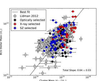
Figure 3: The correlation between the mass of the BCG, and the mass of the cluster at the time at which it was observed. Note that all cluster masses are measured as $M_{200}$.

The correlation between BCG stellar mass and the mass of the host cluster is shown in Figure 3. The positive correlation between the two variables is quite clear - a power law fit to the relation of the form ${M}_{\bf BCG}=\beta{M}_{\bf Cluster}^{\alpha}$ results in a best fit index of $\alpha=0.64\pm 0.03$, similar to that found by Lidman et al. (2012). For the BCGs from the RELICS sample, we have coloured the points based on the selection method of the host clusters. Here one sees that the X-ray selected clusters tend to be larger, and therefore also host larger BCGs, while SZ selected clusters are smaller, with smaller BCGs. Interestingly, the optically selected clusters seem to host smaller BCGs for the given cluster mass.

4 Analysis

Our method of computing the stellar mass growth of BCGs involves comparing the median mass of BCGs in low- and high-redshift samples. The positive correlation between BCG and cluster mass, as shown in Figure 3, highlights the need to account for cluster mass when making a measurement of the mass differences of BCGs in different redshift intervals.

4.1 Accounting for Cluster Masses

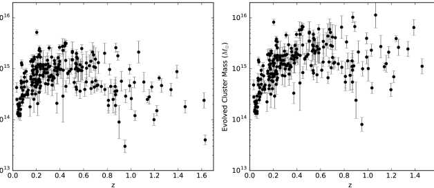
Figure 4: The distribution of cluster masses as a function of redshift. Left: Masses at the epoch the clusters were observed. Right: Masses by the present day ($z=0$). A number of selection effects are visible in these plots. The most massive clusters are under-represented at lower redshifts. Similarly, the least massive clusters are under-represented at high redshifts.

To make an unbiased comparison of the stellar mass of BCGs over different redshift intervals, we follow the procedure outlined in L12. To guarantee that BCGs originating from like-sized clusters are compared with each other, we ensure that during any comparison between BCGs in different redshift bins, the two samples have matching cluster mass distributions. Because clusters observed at high redshift will grow in mass over time, it is necessary that the samples are matched based on their evolved cluster masses, rather than simply those measured at the cluster redshift. To achieve this, L12 first computed the mass each cluster would have by today using the fitting formulae in Fakhouri, Ma & Boylan-Kolchin (2010). The effect this has on the masses is evident from the comparison of the left- and right-hand panels in Figure 4.

After defining two redshift intervals over which to measure the growth of the BCGs, two matched samples are produced by randomly selecting clusters from each of the two intervals without replacement until the cluster mass histograms of the two samples match. The median BCG mass in each sample is then compared. The error in the mass ratio is estimated by repeating the resampling 100 times.

The approach only compares one redshift interval with another interval and not all intervals simultaneously. Unfortunately, there are not enough clusters in the sample to match the cluster mass distributions in all four redshift intervals simultaneously, so we are forced to compare them in pairs. We therefore select one redshift interval as a reference bin (marked in black in Figures 5 and 6), and calculate the growth relative to this point for each of the other bins individually.

Inevitably, some clusters will be rejected if they are over-represented in one redshift interval compared to the other. The bin size selected to match these histograms needs to be small enough to match the overall cluster mass distributions, but large enough so that the rejection of clusters was not unnecessarily large. We applied a bin size of $4\times 10^{14}M_{\odot}$.

4.2 BCG Growth Calculation

Four redshift intervals are considered in our analysis: $0.00<z<0.25$, $0.25<z<0.40$, $0.40<z<0.80$ and $0.80<z<1.60$. We do two comparisons: One using the $0.00<z<0.25$ redshift bin as the comparison point, and another using the $0.25<z<0.40$ redshift bin as the comparison point. This allows us to scale the results at two separate redshifts for easier comparison with models. We present the results of this analysis in Table 7, and in Figures 5 and 6.

4.2.1 The first scaling

Here we scale our data to the low-redshift, $0.0<z<0.25$ bin. The results are shown in the left-hand plots of Figures 5 and 6. In each panel of the graph, the data have been scaled so that the comparison point lies on the model. While the agreement between the data and the DLB07 model is poorer, the agreement between the data, excluding the intermediate-redshift, $0.25<z<0.40$ bin, and the Tonini et al. (2012) model is better. In this model, the BCG accretes stellar mass earlier than in DLB07. The data is also in better agreement with both the observational data from Marchesini et al. (2014) and the semi-empirical model from Shankar et al. (2015).

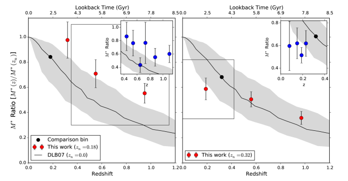
Figure 5: The evolution in BCG stellar mass as a function of redshift normalised to one at $z=0$. The DLB07 model is shown as the solid line and our results are shown as the red, blue and black circles. Red points represent the ratio between the stellar mass of BCGs in these bins and the stellar mass of BCGs in the reference bin (black circles). The left plot shows the results for the first scaling, using a reference bin with mean redshift $z=0.18$, whereas the right plot shows the results for the second scaling with a reference bin with mean redshift $z=0.32$. The grey area shows the error range of the model to which our data has been compared. The points of this work have been rescaled so that the black point lies on the DLB07 model. It is apparent that within each of the scalings, the data disagrees with the model at different redshift intervals. In the low-z scaling, the data above $z=0.2$ all sits above the model. Once the data is scaled to the mid-z interval however, the data above $z=0.2$ agree with the model, however the low-z range lies below the model. As a check that this trend does not simply result from our binning selection, we re-run our analysis for smaller bins in both the high-z and low-z region, and display these results as the blue points in the insets of the left and right plots respectively. Although the errors are larger, it is clear that the trends are the same.

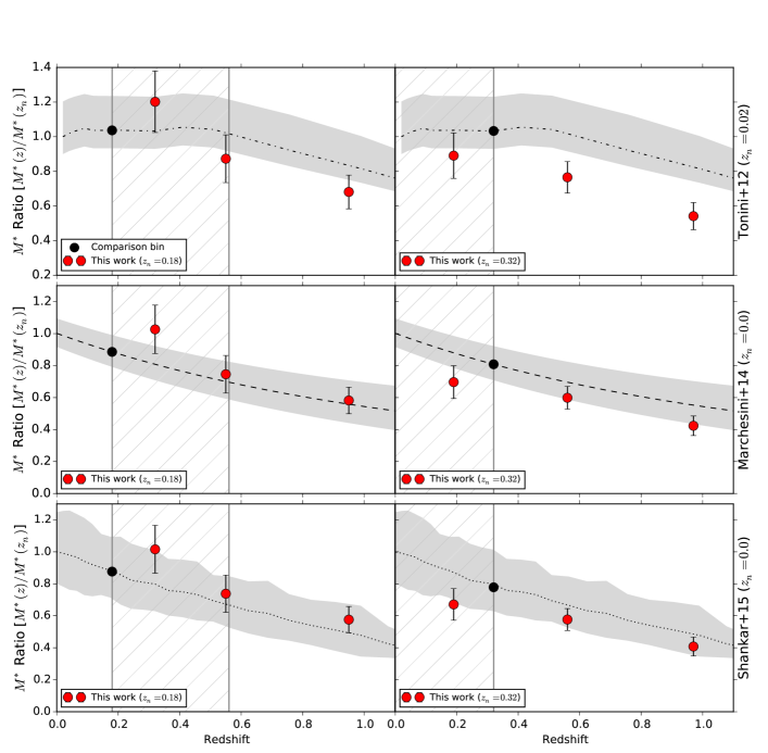
Figure 6: The evolving stellar mass of BCGs with redshift, presented as the ratio of the $M_{BCG}^{*}$ at redshift $z$ with the $M_{BCG}^{*}$ at the comparison redshift $z_{n}$. The red points indicate the stellar mass ratio of the BCGs in their redshift bin, as compared with the comparison bin (black point). In the left column, the ratios are calculated with a low-redshift comparison bin, whereas the ratios in the right column are calculated with a medium-redshift comparison bin. The results have been scaled such that the comparison bin lies on the model (or on the data, in the case of the data from Marchesini et al. (2014)) to which the data are being compared. By changing point at which the difference in stellar mass is calculated, it can be seen that the deviation between data and model may be occurring at either low or medium redshifts, as indicated by the hatched regions. From the top row to the bottom, the three addaitional datasets to which the data are being compared are the simulations model of Tonini et al. (2012); the observational results of Marchesini et al. (2014); and the semi-empirical model of Shankar et al. (2015).

4.2.2 The second scaling

Here we scale our data to the intermediate-redshift, $0.25<z<0.40$ bin. The motivation here is to see if the growth of BCGs stalls at lower redshifts. We first plot this on top of the predictions made by the DLB07 model, as shown in Figure 5.

Although the data match the model very well at higher redshifts, it is clear that the low-redshift point lies below the prediction of the model. We test the robustness of our results around $z\sim 0.2$ by splitting the low redshift bin into four smaller bins, and compare the masses to the intermediate redshift bin. While this causes an increase in the errors of these points due to the smaller sample size of each bin, it is clear to see from the blue points in the inset of the right panel in Figure 5 that the mass of the BCGs in the lower redshift range are consistently lower than what the DLB07 model predicts. This perhaps indicates that the point at which we tie the observations with the model is anomalously high, as there is not a smooth transition between this point and the others at lower redshifts.

To check whether the transition between the high point and those at higher redshifts was smooth, we further split the high redshift bins, as we did for the lower bin. We show these results in the inset within the left panel of Figure 5. This indicates that in the higher bins, the transition is smooth, indicating that the sharper drop in growth below the intermediate redshift bin may be real.

From the perspective of the data, we have no strong reasons to suspect that the data in the intermediate-redshift bin is biased, so we do not choose one interpretation over the other. Instead, we discuss the implications of both in the next section.

Table 7: Results from comparing BCGs masses over different redshift intervals. Columns (3) and (4) give the median redshifts of the lower and upper redshift samples respectively. Column (5) then gives the growth factor between the high- and low-z samples .The bold font values in either column (3) or (4) indicate the redshift bins that were then scaled to the models in Figures 5 and Figure 6.

Low-z Range	High-z Range	Low-z	High-z	Growth	Clusters per bin
(1)	(2)	(3)	(4)	(5)	(6)
Comparing with the $z=0.18$ bin:
0.00-0.25	0.25-0.40	0.18	0.32	0.86$\pm$0.13	33
0.00-0.25	0.40-0.80	0.18	0.55	1.19$\pm$0.19	26
0.00-0.25	0.80-1.60	0.18	0.95	1.52$\pm$0.22	24
Comparing with the $z=0.32$ bin:
0.00-0.25	0.25-0.40	0.19	0.32	0.86$\pm$0.13	33
0.25-0.40	0.40-0.80	0.32	0.56	1.35$\pm$0.16	27
0.25-0.40	0.80-1.60	0.32	0.97	1.91$\pm$0.28	18
Splitting the low-z bin into four smaller bins:
0.00-0.10	0.25-0.40	0.08	0.32	0.88$\pm$0.32	7
0.10-0.17	0.25-0.40	0.15	0.32	0.91$\pm$0.20	13
0.17-0.21	0.25-0.40	0.19	0.32	0.76$\pm$0.10	18
0.21-0.25	0.25-0.40	0.23	0.32	0.91$\pm$0.17	14
Splitting the high-z bins into six smaller bins:
0.25-0.40	0.40-0.50	0.18	0.44	1.04$\pm$0.26	8
0.25-0.40	0.50-0.60	0.18	0.54	1.09$\pm$0.28	9
0.25-0.40	0.60-0.70	0.18	0.65	1.91$\pm$0.48	7
0.25-0.40	0.70-0.80	0.18	0.73	1.08$\pm$0.44	4
0.25-0.40	0.80-1.00	0.18	0.88	1.50$\pm$0.36	14
0.25-0.40	1.00-1.20	0.18	1.1	1.38$\pm$0.30	6

5 Discussion

5.1 Systematic Uncertainties in the Analysis

The points in Figures 5 and 6, were computed using the BC03 stellar population synthesis model and a Chabrier initial mass function (IMF). However, some of the models, plotted as dotted lines in Figure 6, use different stellar population synthesis models. For example, the models of Tonini et al. (2012) use the models from Maraston (2005), which have a strong post-AGB phase. Hence, we need to make sure that the differences between the models and the data are not driven by some of these differences.

We compared a number of models, e.g. models that use a Chabrier IMF with models that use a Salpeter IMF, and models from Maraston (2005) with BC03 models. We find that, while the ratio in the stellar masses of the two models can vary by 25% from the redshift of formation to today, this ratio varies by only a few percent over the redshift range of interest in this paper (i.e. $z\sim 1.6$ to $z\sim 0$). Hence, the differences in Figure 6 between the data and the models are not driven by the assumptions that went into the models.

We additionally checked to see whether the selection method of the clusters has an impact on the measured growth factor. To do this, we measured the growth over two bins ($0<z<0.4$ and $0.4<z<1.6$) for all the data, and then individually for those BCGs from X-ray selected clusters, and also those from Sunyaev-Zel’Dovich selected clusters. We note that the results all agree within error, and that there is therefore no bias as a result of selection. Due to low numbers of optically selected clusters at high redshift, we were unable to carry out this same check for this method of selection.

5.2 The Growth of Clusters and their BCG

In the flat $\Lambda$CDM model, a $10^{15}M_{\odot}$ cluster at $z=0$ is expected to have grown by a factor of about 10 since $z=2$, as shown in Figure 7. Since $z=1$, it is expected that the cluster has grown by a factor of about 3. Observationally, we find that the stellar masses of BCGs grow by a factor of about 2. Hence, over this redshift interval, the cluster grows more quickly than the central BCG. There are a couple of reasons for this.

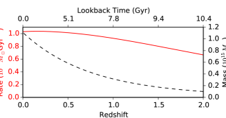
Figure 7: The mass (dashed) and mass accretion rate (red) of a galaxy cluster with a mass of $1\times 10^{14}M_{\odot}$ at $z=2$, according to the mean cluster accretion rate equation of Fakhouri, Ma & Boylan-Kolchin (2010). Note that the cluster accretion rate is roughly constant over time, especially since $z=0.5$.

Firstly, as the cluster grows and becomes larger, the timescale for infalling galaxies to reach the BCG increases. Galaxies that enter the cluster via the outskirts will feel a frictional drag (termed dynamical friction) from the wake they create as they move in the cluster. Over time, dynamical friction brings them closer to the core, and at some point they will merge with the central galaxy. The timescale of this process is (Binney and Tremaine, 1987):

$$t_{\mbox{fric}}=\frac{2.34}{\ln\Lambda}\frac{\sigma_{M}^{2}}{\sigma_{S}^{3}}r_{i}$$ (4)

where $\sigma_{M}$ is the velocity dispersion of the central galaxy, and $\sigma_{S}$ is the velocity dispersion of the satellite; $r_{i}$ represents the radius from which the satellite is spiralling in, and ln $\Lambda$ is the Coulomb logarithm.

For a satellite of a given mass, the timescale is proportional to the halo mass to the two-thirds power and to the radius of the cluster, both of which are increasing in time. The net effect is that it takes longer for material entering the cluster to reach its centre. This, combined with the relatively flat accretion rate (see Figure 7), results in less material reaching the cluster centre as the cluster gets bigger.

The dynamical friction timescale is explicitly included in models that study the growth of BCGs (DLB07, Shankar et al., 2015). Differences in the growth rate of BCGs between models and the data may be due to the way the dynamical friction formula is used in the models. By reducing this time scale by one-third, Shankar et al. (2015) was able to increase the amount of stellar material accreted by BCGs from $z=1$ to today by $\sim 20$%.

Secondly, as an infalling satellite moves through the cluster, tidal stripping as a result of interactions with surrounding objects will occur. As clusters get larger, the number of interactions an infalling satellite will experience will also increase. If the amount of stellar stripping experienced by the infalling satellite is the same per interaction, then by the time the satellite has fallen sufficiently far into the cluster to merge with the BCG, the amount of remaining stellar mass within the satellite available to be accreted by the BCG is less in more massive clusters. Some models set the amount of stripping to zero (Shankar et al., 2015); others do not include it all. Hence, discrepancies between the data and the models may be due to the way tidal striping is included in the model.

Other effects, not captured fully in the data, may contribute to differences between models and the data. In recent work, Burke, Hilton & Collins (2015) have shown that the intra-cluster light (ICL) grows substantially below a redshift of $z\sim 0.4$. It therefore seems reasonable to posit that most of the mass that reaches the cluster core below $z=0.3$ ends up in the ICL and not the BCG. As local BCGs are already quite large, most mergers that occur would be minor mergers. Since minor mergers do not affect the inner cores of the progenitor galaxies, the infalling stars would be inclined to stay on the outskirts of the BCG, and hence contribute to the ICL.

Measuring the amount of material in the ICL is a challenging observation, especially in the K band, where it is several orders of magnitude fainter than the night sky. As mentioned in Section 2.4, MAG_AUTO does not recover the full amount of galaxy light, indicating that light in the outskirts of the galaxy is being neglected by the aperture treatment of MAG_AUTO. An alternative approach to reconciling observations with simulations may be to extend the simulations, so that one creates simulated images, as has been recently done in the Illustris simulation. This would enable one to make the exact same measurement on the simulated image and the real data, thus circumventing some of the biases in the comparison.

In the previous section, we found that we had good agreement with more recent models in the literature (for example, Shankar et al., 2015), if we anchored the data to the models at the low-redshift end. One would then interpret the excess in the intermediate-redshift bin as a slight anomaly.

If one instead anchors the data to the models at the intermediate-redshift bin, we find that we have poorer agreement with the more recent models and better agreement with the DLB07 model, but only in the higher redshift bins. The low redshift point (see right panel of Figure 5) falls well short of the model.

We do not discount either interpretation, as there are no reasons to believe that the clusters in the intermediate-redshift bin lead to a biased measurement in that bin. However, if the latter interpretation is correct, it would mean that the stellar material that contributes to the build-up of mass predicted by the DLB07 model at late times must be done in such a way that it and some of the stellar material that is already in the BCG are distributed outside the apertures that we use to measure fluxes in the Ks-band. This can only happen if the profile of the BCG changes as well.

6 Summary and Conclusions

We have added a sample of 102 BCGs with known cluster masses to an existing sample of 155 BCGs to create a BCG sample spanning the redshift range $0.04<z<1.63$. We use this sample to study the stellar mass growth of BCGs.

We find that the build-up of stellar mass of BCGs from $z\sim 1$ to today, as inferred from the observer-frame Ks band, is broadly consistent with predictions from recent semi-analytic and semi-empirical models.

The BCGs in the very lowest redshift bin have a lower stellar mass than the median-redshift bin, providing tentative evidence that the stellar mass growth rate of BCGs may be slowing.

In order to better constrain the growth rate at lower redshifts, it will be necessary to increase the number of BCGs and to better match the methods used to to derive masses from observations and theoretical models.

7 Acknowledgements

The authors would like to thank the referee for his constructive comments, and whose suggestions have helped make this study a more cohesive analysis. SB acknowledges the help and suggestions of S. Brough and P. Oliva-Altamirano, and the support of the AAO Honours/Masters Scholarship. DM, ZCM, CW, and NK acknowledge the support of the Research Corporation for Science Advancement’s Cottrell Scholarship. JvdS is funded under Bland-Hawthorn’s ARC Laureate Fellowship (FL140100278). ZCM gratefully acknowledges support from the John F. Burlingame and the Kathryn McCarthy Graduate Fellowships in Physics at Tufts University.

This work is based in part on observations taken at the European Southern Observatory New Technology Telescope (ESO programs 092.A-0857 and 094.A-0531), and also on observations taken with the WYIN telescope at the Kitt Peak National Observatory. Additionally, we made use of the ESO Science Archive Facility.

We have used Python, in particular the packages numpy, scipy and astropy, for the data analysis, and matplotlib (Hunter, 2007) for the generation of the plots used within this paper.

Table 8: BCG results.
Redshift sources as given in Table 2
Cluster mass proxy sources: (1) Mann & Ebeling (2012) (2) Mantz et al. (2010) (3) Menanteau et al. (2013) (4) Ebeling et al. (2007) (5) Menanteau et al. (2010) (6) Mahdavi et al. (2013) (7) Piffaretti et al. et al. (2011) (8) Henry et al. (1992) (9) Ebeling et al. (1998) (10) Maughan et al. (2012) (11) Benson et al. (2013) (12) Buddendiek et al. (2015) (13) Hasselfield et al. (2013)
* Magnitude errors stated are those reported by SExtractor.
$\star$ BCG masses are uncertain by $\sim 20\%$.
$\dagger$ All cluster masses are measured to $M_{200}$.

Cluster	$z_{spec}$	$z_{phot}$	z-Source	RA	Dec	BCG Ks-Mag *	BCG Mass $\star$	Cluster Mass $\dagger$	Cluster Mass Proxy	Source
							$\times 10^{12}M_{\odot}$	$\times 10^{15}M_{\odot}$
SPT-CL-J0000-5748	0.702	…	(20)	00:01:0.060	-57:48:33.43	$15.047\pm 0.017$	$1.065$	$0.59\pm 0.10$	SZ Y Parameter	(11)
MACS-J0011.7-1523	0.379	…	(18)	00:11:42.82	-15:23:21.07	$14.914\pm 0.004$	$0.355$	$1.00\pm 0.25$	X-ray Luminosity	(1)
MACS-J0014.3-3022	0.308	…	(1)	00:14:15.82	-30:22:14.4	$12.669\pm 0.003$	$1.743$	$2.57\pm 0.34$	Gas Mass	(2)
MACS-J0014.3-3022	0.308	…	(1)	00:14:17.26	-30:22:34.8	$12.927\pm 0.002$	$1.375$	$2.57\pm 0.34$	Gas Mass	(2)
ACT-CL-J0014.9-0057	0.533	…	(7)	00:14:54.10	-00:57:7.470	$15.081\pm 0.013$	$0.627$	$1.28\pm 0.74$	X-ray Luminosity	(3)
C1G-J001640.6-130644	…	0.700	(21)	00:16:40.71	-13:06:43.7	$16.160\pm 0.220$	$0.484$	$1.55\pm 1.06$	X-ray Luminosity	(12)
ACT-CL-J0017.6-0051	0.211	…	(7)	00:17:37.61	-00:52:41.79	$13.796\pm 0.008$	$0.301$	$0.21\pm 0.15$	X-ray Luminosity	(3)
ACT-CL-J0018.2-0022	…	0.75	(3)	00:18:14.21	-00:22:32.18	$16.066\pm 0.029$	$0.469$	$0.45\pm 0.13$	S-Z Parameter	(13)
MACS-J0025.4-1222	0.5843	…	(1)	00:25:27.42	-12:22:22.76	$15.896\pm 0.017$	$0.351$	$0.92\pm 0.50$	X-ray Temperature	(4)
MACS-J0025.4-1222	0.5843	…	(1)	00:25:33.01	-12:23:16.26	$15.50\pm 0.014$	$0.505$	$0.92\pm 0.50$	X-ray Temperature	(4)
MACS-J0032.1+1808	…	0.398	(22)	00:32:9.380	+18:06:56.17	$14.560\pm 0.013$	$0.569$	…	…	…
MACS-J0033.8-0751	…	0.3	(22)	00:33:53.14	-07:52:10.13	$14.470\pm 0.011$	$0.332$	…	…	…
MACS-J0034.4+0225	…	0.35	(22)	00:34:28.15	+02:25:22.84	$15.020\pm 0.004$	$0.275$	…	…	…
MACS-J0034.9+0234	…	…	…	00:34:58.03	+02:33:33.53	$14.159\pm 0.004$	…	…	…	…
MACS-J0035.4-2015	0.352	…	(1)	00:35:26.20	-20:15:42.19	$14.165\pm 0.005$	$0.606$	$0.93\pm 0.23$	X-ray Luminosity	(1)
Abell68	0.255	…	(12)	00:37:06.87	+09:09:25.50	$13.418\pm 0.004$	$0.625$	$1.11\pm 0.17$	Gas Mass	(2)
SMACS-J0040.8-4407	…	0.4	(14)	00:40:49.97	-44:07:50.2	$14.414\pm 0.006$	$0.651$	…	…	…
C1G-J005805.6+003058	0.662	…	(21)	00:58:05.71	+00:30:58.2	$16.565\pm 0.220$	$0.232$	$1.41\pm 0.92$	X-ray Luminosity	(12)
ACT-CL-J0104.8+0002	0.277	…	(7)	01:04:55.35	+00:03:36.41	$13.749\pm 0.004$	$0.547$	$0.51\pm 0.26$	X-ray Luminosity	(3)
MACS-J0110.1+3211	…	…	…	01:10:7.190	+32:10:48.68	$14.335\pm 0.004$	…	…	…	…
ACT-CL-J0119.9+0055	…	0.72	(3)	01:19:58.15	+00:55:34.03	$16.075\pm 0.004$	$0.44$	$0.48\pm 0.12$	S-Z Parameter	(13)
ACT-CL-J0127.2+0020	0.379	…	(7)	01:27:16.64	+00:20:41.18	$14.363\pm 0.005$	$0.59$	$0.77\pm 0.41$	X-ray Luminosity	(3)
C1G-J013710.4-103423	…	0.575	(21)	01:37:10.55	-10:34:22.1	$15.265\pm 0.220$	$0.625$	$0.93\pm 0.64$	X-ray Luminosity	(12)
RX-J0142.0-2131	…	0.28	(7)	01:42:03.42	+21:31:17.0	$14.280\pm 0.007$	$0.336$	…	…	…
ACT-CL-J0145-5301	0.118	…	(15)	01:45:3.590	-53:01:23.13	$12.798\pm 0.016$	$0.332$	$0.57\pm 0.21$	X-ray Luminosity	(5)
MACS-J0150.3-1005	0.365	…	(12)	01:50:21.27	-10:05:30.19	$13.730\pm 0.006$	$1.057$	…	…	…
ACT-CL-J0152.7+0100	0.23	…	(7)	01:52:41.97	+01:00:26.01	$12.964\pm 0.012$	$0.791$	$0.75\pm 0.30$	X-ray Luminosity	(3)
ACT-CL-J0156.4-0123	…	0.45	(3)	01:56:24.29	-01:23:17.28	$14.055\pm 0.003$	$1.176$	$0.45\pm 0.13$	S-Z Parameter	(13)
ACT-CL-J0206.2-0114	0.676	…	(7)	02:06:13.14	-01:14:59.94	$16.432\pm 0.004$	$0.28$	$2.13\pm 1.16$	X-ray Luminosity	(3)
ACT-CL-J0215-5212	0.48	…	(17)	02:15:12.33	-52:12:25.4	$15.177\pm 0.012$	$0.467$	$0.90\pm 0.69$	X-ray Luminosity	(5)
ACT-CL-J0223.1-0056	0.663	…	(7)	02:15:28.49	+00:30:37.52	$15.971\pm 0.003$	$0.428$	$0.41\pm 0.12$	S-Z Parameter	(13)
ACT-CL-J0218.2-0041	0.672	…	(3)	02:18:17.61	-00:41:38.73	$16.320\pm 0.006$	$0.31$	$0.55\pm 0.12$	S-Z Parameter	(13)
ACT-CL-J0219.8+0022	0.537	…	(3)	02:19:50.42	+00:22:14.7	$15.689\pm 0.220$	$0.358$	$0.44\pm 0.13$	S-Z Parameter	(13)
ACT-CL-J0219.9+0129	…	0.35	(3)	02:19:52.16	+01:29:52.4	$14.432\pm 0.220$	$0.473$	$0.66\pm 0.46$	X-ray Luminosity	(3)
ACT-CL-J0221.5-0012	0.589	…	(7)	02:21:36.51	-00:12:22.37	$15.902\pm 0.025$	$0.375$	$1.08\pm 0.86$	X-ray Luminosity	(3)
ACT-CL-J0232-5257	0.556	…	(17)	02:32:42.72	-52:57:22.59	$15.072\pm 0.022$	$0.691$	$0.98\pm 0.71$	X-ray Luminosity	(5)
ACT-CL-J0232-5257	0.556	…	(17)	02:32:49.42	-52:57:11.48	$15.349\pm 0.019$	$0.536$	$0.98\pm 0.71$	X-ray Luminosity	(5)
ACT-CL-J0235-5121	0.278	…	(17)	02:35:45.26	-51:21:4.770	$13.143\pm 0.035$	$0.956$	$1.20\pm 0.56$	X-ray Luminosity	(5)
ACT-CL-J0237-4939	0.334	…	(17)	02:37:1.670	-49:38:9.680	$14.063\pm 0.014$	$0.567$	$0.59\pm 0.33$	X-ray Luminosity	(5)
Abell370	0.375	…	(7,12)	02:39:51.90	-01:35:14.72	$14.254\pm 0.009$	$0.652$	$0.89\pm 0.68$	X-ray Luminosity	(3)
Abell370	0.375	…	(7,12)	02:39:52.31	-01:35:52.15	$13.987\pm 0.008$	$0.834$	$0.89\pm 0.68$	X-ray Luminosity	(3)
MACS-J0242.5-2132	0.314	…	(1)	02:42:35.91	-21:32:25.8	$13.614\pm 0.005$	$0.857$	$1.12\pm 0.19$	Gas Mass	(2)

Cluster	$z_{spec}$	$z_{phot}$	z-Source	RA	Dec	BCG Ks-Mag *	BCG Mass $\star$	Cluster Mass	Cluster Mass Proxy	Source
							$\times 10^{12}M_{\odot}$	$\times 10^{15}M_{\odot}$
ACT-CL-J0245.8-0042	0.179	…	(8)	02:45:51.74	-00:42:16.34	$13.372\pm 0.016$	$0.354$	$0.25\pm 0.21$	X-ray Luminosity	(3)
ACT-CL-J0250.1+0008	…	0.78	(3)	02:50:8.40	+00:08:16.22	$16.360\pm 0.003$	$0.38$	$0.39\pm 0.12$	S-Z Parameter	(13)
ACT-CL-J0256+0006	0.363	…	(8)	02:56:30.84	+00:06:03.3	$14.747\pm 0.008$	$0.414$	$1.06\pm 0.45$	X-ray Luminosity	(3)
ACT-CL-J0256+0006	0.363	…	(8)	02:56:33.76	+00:06:28.8	$15.067\pm 0.011$	$0.308$	$1.06\pm 0.45$	X-ray Luminosity	(3)
MACS-J0257.1-2325	0.505	…	(1)	02:57:8.760	-23:26:4.890	$14.686\pm 0.007$	$0.817$	$2.18\pm 1.19$	X-ray Temperature	(4)
MACS-J0257.1-2325	0.505	…	(1)	02:57:8.790	-23:26:4.930	$14.510\pm 0.002$	$0.96$	$2.18\pm 1.19$	X-ray Temperature	(4)
ACT-CL-J0301.6+0155	0.167	…	(9)	03:01:38.20	+01:55:14.66	$13.084\pm 0.006$	$0.461$	$0.54\pm 0.25$	X-ray Luminosity	(3)
ACT-CL-J0304-4921	0.392	…	(17)	03:04:16.18	-49:21:26.3	$14.263\pm 0.007$	$0.748$	$1.22\pm 0.58$	X-ray Luminosity	(5)
SMACS-J0304.3-4401	…	0.52	(17)	03:04:16.86	-44:01:31.5	$15.035\pm 0.010$	$0.654$	…	…	…
SMACS-J0304.3-4401	…	0.52	(17)	03:04:21.09	-44:02:37.51	$15.064\pm 0.014$	$0.637$	…	…	…
ACT-CL-J0326.8-0043	0.448	…	(9)	03:26:49.94	-00:43:51.61	$14.339\pm 0.007$	$0.905$	$1.46\pm 0.75$	X-ray Luminosity	(3)
ACT-CL-J0330-5227	0.44	…	(9,10)	03:30:56.96	-52:28:13.2	$14.274\pm 0.008$	$0.958$	$2.86\pm 0.97$	X-ray Luminosity	(5)
ACT-CL-J0346-5438	0.53	…	(17)	03:46:55.48	-54:38:55.0	$15.063\pm 0.014$	$0.637$	$0.99\pm 0.54$	X-ray Luminosity	(5)
ACT-CL-J0348+0029	0.297	…	(17)	03:48:36.71	+00:29:32.9	$14.496\pm 0.009$	$0.324$	$0.50\pm 0.30$	X-ray Luminosity	(3)
ACT-CL-J0348-0028	0.345	…	(17)	03:48:38.25	-00:28:08.6	$13.869\pm 0.003$	$0.795$	$0.69\pm 0.40$	X-ray Luminosity	(3)
MACS-J0358.8-2955	0.425	…	(1)	03:58:54.09	-29:55:30.8	$14.415\pm 0.016$	$0.746$	$2.3\pm 0.67$	Gas Mass	(2)
MACS-J0416.1-2403	0.40	…	(2)	04:16:09.15	-24:04:02.1	$14.084\pm 0.007$	$0.882$	$0.97\pm 0.24$	X-ray Luminosity	(1)
MACS-J0417.5-1154	0.443	…	(2)	04:17:34.49	-11:54:34.3	$13.877\pm 0.004$	$1.385$	$3.22\pm 0.39$	Gas Mass	(2)
Abell496	0.0328	…	(7)	04:33:37.84	-13:15:43.10	$10.743\pm 0.001$	$0.185$	$0.43\pm 0.11$	X-ray Luminosity	(7)
ACT-CL-J0438-5419	0.421	…	(17)	04:38:17.68	-54:19:20.5	$14.045\pm 0.005$	$1.049$	$2.75\pm 1.16$	X-ray Luminosity	(5)
SMACS-J0439-4600	…	…	…	04:39:13.91	-46:00:48.55	$14.271\pm 0.010$	…	…	…	…
MS-0440+0204	0.197	…	(5)	04:43:16.14	+02:10:02.4	$13.180\pm 0.002$	$0.53$	$0.44\pm 0.11$	X-ray Luminosity	(8)
MS-0440+0204	0.197	…	(5)	04:43:16.29	+02:10:04.6	$13.230\pm 0.001$	$0.506$	$0.44\pm 0.11$	X-ray Luminosity	(8)
MACS-J0449-2848	…	…	…	04:49:20.76	-28:49:08.19	$14.916\pm 0.009$	…	…	…	…
MACS-J0451.6-0305	0.5386	…	(5)	04:54:10.84	-03:00:51.5	$15.691\pm 0.015$	$0.39$	$1.22\pm 0.30$	X-ray Luminosity	(1)
MACS-J0454.1-0300	0.5377	…	(6)	04:54:16.12	-02:59:26.4	$15.367\pm 0.008$	$0.525$	$1.06\pm 0.58$	X-ray Temperature	(4)
Abell520	0.205	…	(2)	04:54:3.810	+02:53:32.05	$13.497\pm 0.028$	$0.396$	$1.04\pm 0.26$	X-ray Luminosity	(1)
ACT-CL-J0516-5430	0.294	…	(23)	05:16:37.35	-54:30:1.520	$13.30\pm 0.002$	$0.974$	$1.47\pm 0.57$	X-ray Luminosity	(5)
SPT-CL-J0553-5005	0.881	…	(24)	05:33:37.50	-50:06:4.750	$16.826\pm 0.010$	$0.305$	$0.37\pm 0.08$	SZ Y Parameter	(11)
SPT-CL-J0546-5345	1.066	…	(27)	05:46:37.66	-53:45:31.08	$17.062\pm 0.002$	$0.333$	$2.13\pm 1.37$	X-ray Luminosity	(5)
MACS-J0553.4-3342	0.407	…	(12)	05:53:19.35	-33:42:27.4	$15.228\pm 0.005$	$0.308$	…	…	…
MACS-J0553.4-3342	0.407	…	(12)	05:53:25.77	-33:42:28.0	$14.534\pm 0.010$	$0.583$	…	…	…
SMACS-J0600.2-2008	…	0.46	(12)	06:00:08.18	-20:08:09.0	$14.965\pm 0.008$	$0.509$	…	…	…
SMACS-J0600-4353	…	…	…	06:00:13.05	-43:53:30.47	$14.305\pm 0.003$	…	…	…	…
SMACS-J0600.2-2008	…	0.46	(12)	06:00:16.83	-20:06:55.7	$14.614\pm 0.008$	$0.702$	…	…	…
ACT-CL-J0616-5227	0.684	…	(17)	06:16:33.92	-52:27:09.9	$15.001\pm 0.011$	$1.045$	$1.88\pm 0.92$	X-ray Luminosity	(5)
ACT-CL-J0641-4949	0.146	…	(9,11)	06:41:37.81	-49:46:54.5	$12.735\pm 0.003$	$0.487$	$0.18\pm 0.10$	X-ray Luminosity	(5)
ACT-CL-J0645-5413	0.167	…	(15)	06:45:29.48	-54:13:36.93	$12.624\pm 0.005$	$0.704$	$1.13\pm 0.36$	X-ray Luminosity	(5)
ACT-CL-J0707-5522	0.296	…	(26)	07:07:04.70	-55:23:08.5	$13.368\pm 0.005$	$0.916$	$1.24\pm 0.55$	X-ray Luminosity	(5)
SMACS-J0723.3-7327	…	0.39	(16)	07:23:18.46	-73:27:17.0	$15.062\pm 0.043$	$0.358$	…	…	…
C1G-J080434.9+330509	0.552	…	(21)	08:04:35.12	+33:05:8.430	$15.032\pm 0.004$	$0.717$	$0.91\pm 0.59$	X-ray Luminosity	(12)
Abell644	0.0704	…	(7)	08:17:25.62	-07:30:45.40	$11.818\pm 0.002$	$0.27$	$0.57\pm 0.14$	X-ray Luminosity	(7)
MACSJ-0845.4+0327	…	…	…	08:45:27.76	+03:27:38.93	$14.106\pm 0.030$	…	…	…	…
MACS-J0850.1+3604	0.378	…	(19)	08:50:7.840	+36:04:11.48	$14.356\pm 0.037$	$0.594$	…	…	…
Abell750	0.18	…	(12)	09:09:12.77	+10:58:28.72	$13.274\pm 0.003$	$0.388$	…	…	…
MACS-J0911.2+1746	0.5049	…	(6)	09:11:11.55	+17:46:28.7	$15.111\pm 0.016$	$0.552$	$1.51\pm 0.82$	X-ray Temperature	(4)
C1G-J094811.6+290709	0.778	…	(21)	09:48:11.50	+29:07:12.15	$16.158\pm 0.007$	$0.458$	$2.02\pm 1.18$	X-ray Luminosity	(12)
MACS-J0949.8+1708	0.384	…	(1)	09:49:51.81	+17:07:9.580	$14.326\pm 0.008$	$0.612$	$1.65\pm 0.34$	Gas Mass	(2)
Abell901	0.170	…	(1)	09:56:29.92	-10:05:42.26	$14.521\pm 0.007$	$0.123$	…	…	…
Abell963	0.206	…	(1)	10:17:3.660	+39:02:49.71	$12.651\pm 0.006$	$0.863$	$0.87\pm 0.47$	X-ray Temperature	(6)
MACS-J1105.7-1014	0.466	…	(1)	11:05:46.82	-10:14:46.1	$14.491\pm 0.008$	$0.878$	$0.83\pm 0.20$	X-ray Luminosity	(1)

Cluster	$z_{spec}$	$z_{phot}$	z-Source	RA	Dec	BCG Ks-Mag *	BCG Mass $\star$	Cluster Mass	Cluster Mass Proxy	Source
							$\times 10^{12}M_{\odot}$	$\times 10^{15}M_{\odot}$
MACS-J1108.8+0906	0.466	…	(19)	11:08:55.34	+09:06:3.160	$14.685\pm 0.001$	$0.734$	$0.80\pm 0.20$	X-ray Luminosity	(1)
Abell1204	0.171	…	(12)	11:13:20.51	+17:35:41.00	$13.40\pm 0.004$	$0.344$	$0.92\pm 0.23$	X-ray Luminosity	(9)
MACS-J1115.8+0129	0.355	…	(12)	11:15:51.93	+01:29:55.2	$14.405\pm 0.009$	$0.487$	$1.26\pm 0.17$	Gas Mass	(2)
MACS-J1206.2-0847	0.439	…	(1)	12:06:12:16	-08:48:03.1	$14.618\pm 0.007$	$0.698$	$2.80\pm 0.44$	Gas Mass	(2)
Abell1553	0.165	…	(7)	12:30:48.86	+10:32:47.30	$12.385\pm 0.003$	$0.877$	$0.92\pm 0.23$	X-ray Luminosity	(9)
Abell1634	0.196	…	(12)	12:54:01.85	-06:42:14.00	$13.481\pm 0.006$	$0.401$	$0.60\pm 0.15$	X-ray Luminosity	(7)
MACS-J1311.0-0311	0.494	…	(12)	13:11:01.77	-03:10:40.5	$14.977\pm 0.010$	$0.625$	$0.98\pm 0.24$	X-ray Luminosity	(1)
Abell1689	0.183	…	(7)	13:11:27.20	-01:18:45.50	$13.136\pm 0.003$	$0.44$	$1.54\pm 0.22$	Gas Mass	(2)
Abell1758	0.279	…	(19)	13:32:38.40	+50:33:35.61	$13.877\pm 0.011$	$0.486$	$0.83\pm 0.20$	X-ray Luminosity	(1)
Abell1758	0.279	…	(19)	13:32:52.04	+50:31:34.62	$14.178\pm 0.016$	$0.369$	$0.83\pm 0.20$	X-ray Luminosity	(1)
MACS-J1347.5-1144	0.451	…	(1)	13:47:29.38	-11:45:06.0	$14.449\pm 0.010$	$0.817$	$3.16\pm 0.44$	Gas Mass	(2)
MACS-J1347.5-1144	0.451	…	(1)	13:47:30.61	-11:45:08.23	$14.405\pm 0.009$	$0.851$	$3.16\pm 0.44$	Gas Mass	(2)
Abell1835	0.253	…	(1)	14:01:02.11	+02:52:43.10	$13.193\pm 0.002$	$0.769$	$1.12\pm 0.61$	X-ray Temperature	(6)
MACS-J1427+44	0.487	…	(19)	14:27:16.17	+44:07:31.16	$14.638\pm 0.006$	$0.769$	…	…	…
Abell1942	0.224	…	(7)	14:38:21.88	+03:40:13.10	$13.178\pm 0.003$	$0.65$	$0.34\pm 0.19$	X-ray Temperature	(6)
Abell1994	0.22	…	(12)	14:56:13.47	-05:48:55.80	$13.939\pm 0.005$	$0.322$	$0.60\pm 0.15$	X-ray Luminosity	(7)
MACS-J1652.3+5534	…	…	…	16:52:18.67	+55:34:58.54	$14.547\pm 0.009$	…	…	…	…
RX-J1720.1+2638	0.164	…	(12)	17:20:10.02	+26:37:32.1	$13.381\pm 0.004$	$0.35$	$1.51\pm 0.37$	X-ray Luminosity	(9)
MACS-J1752.0+4440	0.366	…	(13)	17:51:53.38	+44:39:13.4	$15.101\pm 0.011$	$0.299$	…	…	…
MACS-J1931.8-2634	0.352	…	(1)	19:31:49.65	-26:34:33.0	$14.178\pm 0.009$	$0.599$	$1.45\pm 0.23$	Gas Mass	(2)
ACT-CL-J2025.2+0030	…	0.34	(3)	20:25:013.0	+00:31:38.76	$14.414\pm 0.002$	$0.481$	$0.67\pm 0.15$	S-Z Parameter	(13)
ACT-CL-J2050.5-0055	0.622	…	(3)	20:50:29.73	-00:55:40.38	$16.086\pm 0.006$	$0.339$	$0.55\pm 0.12$	S-Z Parameter	(13)
ACT-CL-J2051.1+0056	0.333	…	(7)	20:51:11.09	+00:56:45.92	$13.772\pm 0.003$	$0.742$	$0.48\pm 0.31$	X-ray Luminosity	(3)
ACT-CL-J2055.4+0105	0.408	…	(7)	20:55:23.23	+01:06:7.830	$14.925\pm 0.002$	$0.407$	$0.98\pm 0.52$	X-ray Luminosity	(3)
ACT-CL-J2128.4+0135	0.385	…	(3)	21:28:23.42	+01:35:36.64	$14.264\pm 0.006$	$0.647$	$1.08\pm 0.57$	X-ray Luminosity	(3)
ACT-CL-J2129.6+0005	0.234	…	(7)	21:29:39.95	+00:05:21.32	$13.203\pm 0.004$	$0.635$	$1.23\pm 0.47$	X-ray Luminosity	(3)
ACT-CL-J2130.1+0045	…	0.71	(3)	21:30:8.840	+00:46:48.64	$15.785\pm 0.009$	$0.541$	$0.47\pm 0.13$	S-Z Parameter	(13)
MACS-J2140.1-2339	0.313	…	(3)	21:40:15.03	-23:39:37.8	$13.842\pm 0.003$	$0.694$	$0.69\pm 0.09$	Gas Mass	(2)
C1G-J214826.3-053312	…	0.625	(21)	21:48:26.25	-05:33:11.2	$16.347\pm 0.220$	$0.266$	$1.03\pm 0.68$	X-ray Luminosity	(12)
RX-J2149.3+0951	…	…	…	21:49:19.68	+09:51:36.79	$15.008\pm 0.010$	…	…	…	…
ACT-CL-J2152.9-0114	…	0.69	(4)	21:52:55.65	-01:14:53.20	$16.729\pm 0.003$	$0.226$	$0.44\pm 0.13$	S-Z Parameter	(13)
Abell2390	0.233	…	(1)	21:53:36.80	+17:41:43.60	$13.922\pm 0.004$	$0.327$	$2.22\pm 0.28$	Gas Mass	(2)
Abell3827	0.0993	…	(7)	22:01:53.44	-59:56:42.60	$12.323\pm 0.001$	$0.338$	$0.68\pm 0.17$	X-ray Luminosity	(7)
MACS-J2211.7-0349	0.396	…	(7)	22:11:45.88	-03:49:44.3	$14.143\pm 0.008$	$0.835$	$2.64\pm 0.36$	Gas Mass	(2)
MACS-J2214.9-1359	0.5027	…	(7)	22:14:57.25	-14:00:12.8	$14.938\pm 0.011$	$0.648$	$1.51\pm 0.82$	X-ray Temperature	(4)
ACT-CL-J2220.7-0042	…	0.57	(4)	22:20:47.05	-00:41:54.11	$15.713\pm 0.008$	$0.414$	$0.36\pm 0.14$	S-Z Parameter	(13)
ACT-CL-J2229.2-0004	…	0.61	(4)	22:29:7.540	-00:04:10.50	$15.701\pm 0.002$	$0.451$	$0.39\pm 0.14$	S-Z Parameter	(13)
C1G-J223007.6-080949	0.623	…	(21)	22:30:07.50	-08:09:48.6	$16.128\pm 0.220$	$0.282$	$1.30\pm 0.88$	X-ray Luminosity	(12)
C1G-J223727.5+135523	…	0.700	(21)	22:37:27.54	+13:55:23.5	$16.466\pm 0.220$	$0.239$	$1.06\pm 0.68$	X-ray Luminosity	(12)
MACS-J2241.8+1732	0.3137	…	(23)	22:41:56.32	+17:32:6.980	$14.079\pm 0.002$	$0.558$	…	…	…
CL2244	0.328	…	(23)	22:47:13.38	-02:05:41.40	$14.836\pm 0.009$	$0.278$	…	…	…
MACS-J2248.7-4431	0.3475	…	(23)	22:48:43.99	-44:31:51.1	$13.375\pm 0.004$	$1.253$	…	…	…
ACT-CL-J2253.3-0031	…	0.54	(4)	22:53:24.26	-00:30:30.71	$15.862\pm 0.035$	$0.333$	$0.39\pm 0.13$	S-Z Parameter	(13)
AC114	0.313	…	(4)	22:58:56.33	-34:45:40.4	$14.022\pm 0.003$	$0.588$	…	…	…
ACT-CL-J2302.5+0002	0.52	…	(9)	23:02:35.07	+00:02:34.34	$15.523\pm 0.018$	$0.417$	$0.54\pm 0.13$	S-Z Parameter	(13)
Abell2552	0.302	…	(25)	23:11:33.27	+03:38:5.220	$13.549\pm 0.017$	$0.775$	$1.08\pm 0.27$	X-ray Luminosity	(1)
C1G-J231215.6+035307	0.648	…	(21)	23:12:17.05	+03:53:14.9	$16.029\pm 0.220$	$0.357$	$1.15\pm 0.72$	X-ray Luminosity	(12)
C1G-J231520.6+090711	…	0.725	(21)	23:15:20.57	+09:07:11.9	$16.413\pm 0.220$	$0.266$	$1.32\pm 0.85$	X-ray Luminosity	(12)
Abell2631	0.273	…	(12)	23:37:39.73	+00:16:16.90	$14.237\pm 0.006$	$0.349$	$0.98\pm 0.24$	X-ray Luminosity	(1)
ACT-CL-J2351.7+0009	…	0.99	(3)	23:51:44.70	+00:09:16.27	$16.269\pm 0.004$	$0.623$	$0.46\pm 0.14$	S-Z Parameter	(13)

References

- Abell, Corwin & Olowin (1989) Abell G. O., Corwin H. G. Jr., Olowin R. P., 1989, ApJ, 70, 1
- Aganim et al. (2012) Aghanim N. et al., 2012, A&A, 543, 102
- Applegate et al. (2014) Applegate D. E., von der Linden A., Kelly P. L., Allen M. T., Burchat P. R., Burke D. L., Ebeling H., Mantz A., Morris R. G., 2014, MNRS, 439, 48
- Ascaso et al. (2011) Ascaso B., Aguerri J. A. L., Varela J., Cava A., Bettoni D., Moles M., D’Onofrio M., 2011, ApJ, 726, 69
- Bai et al. (2014) Bai et al., 2014, ApJ, 789, 134
- Benson et al. (2013) Benson B. A. et al., 2013, ApJ, 763, 147
- Bertin & Arnouts (1996) Bertin E., Arnouts S., 1996, A&AS, 117, 393
- Binney and Tremaine (1987) Binney J., Tremaine S., 1987, Galactic Dynamics - Second Edition, Princeton Univ. Press, Princeton, NJ, p650
- Brodwin et al. (2010) Brodwin M., et al. 2010, ApJ, 721, 90
- Brough et al. (2008) Brough S., Couch W. J., Collins C. A., Jarrett T., Burke D. J., Mann R. G., 2008, MNRAS, 385, L103
- Bruzual & Charlot (2003) Bruzual G., Charlot S., 2003, MNRAS, 344, 1000
- Buddendiek et al. (2015) Buddendiek A. et al., 2015, MNRAS, 450, 4248
- Burke, Collins & Mann (2000) Burke D., Collins C., Mann R., 2000, ApJ, 532, 105
- Burke, Hilton & Collins (2015) Burke C., Hilton M., Collins C., 2015, MNRAS, 339, 2353
- Carlstrom et al. (2011) Carlstrom J. E. et al., 2011, PASP, 123, 568
- Chabrier (2003) Chabrier G., 2003, PASP, 115, 763
- Collins et al. (2009) Collins C. A. et al., 2009, Nature, 458, 603
- De Lucia & Blaizot (2007) De Lucia G. and Blaizot J., 2007, MNRAS, 375, 2
- Duffy et al. (2008) Duffy A. R., Schaye J., Kay S. T., Vecchia C. C., 2008, MNRAS, 390, 64
- Ebeling et al. (1998) Ebeling H., Allen S. W., Crawford C. S., Fabian A. C., Edge A. C., Bo H., Voges W., Huchra J. P., 1998, MNRAS, 914, 881
- Ebeling, Edge & Henry (2001) Ebeling H., Edge A. C., Henry J. P., 2001, ApJ, 553, 668
- Ebeling et al. (2007) Ebeling H., Barrett E., Donovan D., Ma C. J., Edge A. C., Speybroeck L. Van, 2007, ApJ, 661, 33
- Ebeling et al. (2010) Ebeling H., Edge A. C., Mantz A., Barrett E., Henry J. P., Ma C. J., Speybroeck L. Van, MNRAS, 93, 83
- Edge (1991) Edge A. C., 1991, MNRAS, 250, 103
- Fakhouri, Ma & Boylan-Kolchin (2010) Fakhouri O., Ma C., Boylan-Kolchin M., 2010, MNRAS, 406, 2267
- Gioia et al. (1998) Gioia I. M., Shaya E. J., Fevre O. Le, Falco E. E., Luppino G. A., Hammer F., 1998, ApJ, 497, 573
- Hasselfield et al. (2013) Hasselfield M. et al., 2013, JCAP, 07, 008
- Henry et al. (1992) Henry J. P., Gioia I. M., Maccacaro T., Morris S. L., Stocke J. T., Wolter A., 1992, ApJ, 386, 408
- Hilton et al. (2013) Hilton M. et al., 2013, MNRAS, 435, 3469
- Hu & Kravtsov (2003) Hu W., Kravtsov A. V., 2003, ApJ, 584, 702
- Hunter (2007) Hunter J. D., 2007, Comput. Sci. Eng., 9, 90
- Inagaki et al. (2014) Inagaki T., Lin Y.-T., Huang H., Hsieh B., Sugiyama N., 2014, MNRAS, 11, 1
- Jones et al. (2009) Jones D. H., et al., 2009, MNRAS, 399, 683
- Kristian, Sandage & Westphal (1978) Kristian J., Sandage A., Westphal J. A., 1978, ApJ, 221, 383
- Kron (1980) Kron R. G., 1980, ApJS, 43, 305
- Laporte et al. (2013) Laporte C. F. P., White S. D. M., Naab T., Gao L., 2013, MNRAS, 435, 901
- Lidman et al. (2008) Lidman C., Rosati P., Tanaka M., Strazzullo V., Demarco R., Mullis C., Ageorges N., Selman F., A&A, 406, 2267
- Lidman et al. (2012) Lidman C. et al., 2012, MNRAS, 427, 550
- Lin et al. (2013) Lin Y.-T., Brodwin M. Gonzalez A. H., Bode P., Eisenhardt P. R. M., Stanford A., Vikhlinin A., 2013, ApJ, 771, 61
- Loh & Strauss (2006) Loh Y.-S., Strauss M., 2006, MNRAS, 366, 373
- Mahdavi et al. (2013) Mahdavi A., Hoekstra H., Babul A., Bildfell C., Jeltema T., Henry J. P., 2013, ApJ, 767, 116
- Mann & Ebeling (2012) Mann A. W., Ebeling H., 2012, MNRAS, 420, 2120
- Mantz et al. (2010) Mantz A., Allen S. W., Ebeling H., Rapetti D., Drlica-Wagner A., 2010, MNRAS, 407, 1773
- Marchesini et al. (2014) Marchesini D., Muzzin A., Stefanon M., Franx M., Brammer G. G., Marsan C. Z., Vulcani B., Fynbo J. P. U., Milvang-Jensen B., Dunlop J. S., Buitrago F., 2014, ApJ, 794, 65
- Marriage et al. (2011) Marriage T. A. et al., 2011, ApJ, 737, 61
- Maughan et al. (2012) Maughan B. J., Giles P. A., Randall S. W., Jones C., Forman W. R., 2012, MNRAS, 421, 1583
- Maraston (2005) Maraston C., 2005, MNRAS, 362, 799
- Menanteau et al. (2010) Menanteau F. et al., 2010, ApJ, 723, 1523
- Menanteau et al. (2013) Menanteau F. et al., 2013, ApJ, 765, 67
- Miexner et al. (2010) Miexner M. et al., 2010, PASP, 122, 451
- Moorwood, Cudy & Lidman (1998) Moorwood A., Cuby J.-G., Lidman C., 1998, Messenger, 91, 9
- Moustakas et al. (2013) Moustakas J., Coil A. L., Aird J., Blanton M. R., Cool R. J., Eisenstein D. J., Wong K. C., Zhu G., Arnouts S., 2013, ApJ, 767, 50
- Navarro, Frenk & White (1997) Navarro J. F., Frenk C. S., White S. D. M., 1997, ApJ, 490, 493
- Oliva-Altamirano et al. (2014) Oliva-Altamirano P. et al., 2014, MNRAS, 440, 762
- Piffaretti et al. et al. (2011) Piffaretti R., Arnaud M., Pratt G. W., Pointecouteau E., Melin J.-B., 2011, A&A, 534, A109
- Ruel et al. (2014) Ruel J. et al., 2014, ApJ, 792, 45
- Shankar et al. (2014) Shankar F. et al., MNRAS, 439, 3189
- Shankar et al. (2015) Shankar F. et al., 2015, ApJ, 802, 73
- Shen et al. (2013) Shen S., Yang X., Mo H., van den Bosch F., More S., 2013, arXiv:1307.5107
- Sifón et al. (2013) Sifón C. et al., 2013, ApJ, 772, 25
- Skrutskie et al. (2006) Skrutskie M. F., et al., AJ, 131, 1163
- Staniszewski et al. (2009) Staniszewski Z. et al., 2009, ApJ, 701, 32
- Story et al. (2011) Story K. et al., 2011, ApJ, 735, L36
- Stott et al. (2008) Stott J. P., Edge A. C., Smith G. P., Swinbank A. M., Ebeling H., 2008, MNRAS, 384, 4
- Stott et al. (2010) Stott J. P. et al., 2010, ApJ, 718, 23
- Stott et al. (2012) Stott J. P. et al., 2012, MNRAS, 422, 2213
- Swetz et al. (2011) Swetx D. S. et al., 2011, ApJS, 194, 41
- Tonini et al. (2012) Tonini C., Bernyk M., Croton D., Maraston C., Thomas D., 2012, ApJ, 759 43
- van der Burg et al. (2015) van der Burg R. F. J., Hoekstra H., Muzzin A., Sifón C., Balogh M. L., McGee S. L., 2015, A&A, 577, A19
- Vanderlinde et al. (2010) Vanderlinde K. et al., 2010, ApJ, 722, 1180
- van Weeren et al. (2012) van Weeren R. J., Bonafede A., Ebeling H., Edge A. C., Brüggen M., Giovannini G., Hoeft M., Röttgering H. J. A., 2012, MNRAS, 425, L36
- von der Linden et al. (2007) von der Linden A., Best P., Kauffmann G., White S., 2007, MNRAS, 379, 867
- von der Linden et al. (2014) von der Linden A. et al., 2014, MNRAS, 439, 2
- Vikhlinin et al. (2009) Vihklinin A. et al., 2009, ApJ, 692, 1033
- Wen & Han (2013) Wen Z. L., Han J. L., 2013, MNRAS, 436, 275
- Werner et al. (2007) Werner N., Churazov E., Finoguenov A., Markevitch M., Burenin R., Kaastra J. S., Böhringer H., 2007, 474, 707
- Whiley et al. (2008) Whiley I. M. et al., 2008, MNRAS, 387, 499
- Williamson et al. (2011) Williamson R. et al., 2011, ApJ, 738, 139.
- Yee, Ellingson & Carlberg (1996) Yee H. K. C., Ellingson E., Carlberg R. G., 1996, ApJS, 102, 269
- Zhang et al. (2015) Zhang, Y. et al. arXiv: 1504.02983