Data-driven Model-independent Searches for Long-lived Particles at the LHC

Abstract

Neutral long-lived particles (LLPs) are highly motivated by many BSM scenarios, such as theories of supersymmetry, baryogenesis, and neutral naturalness, and present both tremendous discovery opportunities and experimental challenges for the LHC. A major bottleneck for current LLP searches is the prediction of SM backgrounds, which are often impossible to simulate accurately. In this paper, we propose a general strategy for obtaining differential, data-driven background estimates in LLP searches, thereby notably extending the range of LLP masses and lifetimes that can be discovered at the LHC. We focus on LLPs decaying in the ATLAS Muon System, where triggers providing both signal and control samples are available at the LHC Run-2. While many existing searches require two displaced decays, a detailed knowledge of backgrounds will allow for very inclusive searches that require just one detected LLP decay. As we demonstrate for the $h\to XX$ signal model of LLP pair production in exotic Higgs decays, this results in dramatic sensitivity improvements for proper lifetimes $\gtrsim 10$ m. In theories of Neutral Naturalness, this extends reach to glueball masses far below the $\bar{b}b$ threshold. Our strategy readily generalizes to other signal models, and other detector subsystems. This framework therefore lends itself to the development of a systematic, model-independent LLP search program, in analogy to the highly successful simplified-model framework of prompt searches.

I Introduction

The discovery of the Higgs boson has filled in the last missing piece of the Standard Model (SM). It also has focused attention on the many open issues the SM does not address, including dark matter, the matter-antimatter asymmetry of our universe, and the naturalness of the electroweak scale in the absence of obvious TeV-scale signals of physics beyond the SM (BSM) to date. Many extensions of the SM that address these issues allow or require for long-lived particles (LLPs) that decay at some macroscopic distance from the pp interaction point. Examples include mini-split supersymmetry (SUSY) Arvanitaki et al. (2013); Arkani-Hamed et al. (2012), gauge mediation Giudice and Rattazzi (1999), RPV SUSY Barbier et al. (2005); Csaki et al. (2014), Stealth SUSY Fan et al. (2011), models of baryogenesis Bouquet and Salati (1987); Campbell et al. (1991); Cui and Sundrum (2013); Barry et al. (2014); Ipek and March-Russell (2016), Hidden Valleys Strassler and Zurek (2007, 2008); Strassler (2006); Han et al. (2008); Strassler (2008a, b), dark photons Curtin et al. (2015); Clarke (2015); Argüelles et al. (2016), and theories of Neutral Naturalness Burdman et al. (2007); Cai et al. (2009); Chacko et al. (2006). The proper decay lengths of such particles can range from the mesoscopic (about $100\mu$m) to on the order of kilometers, far in excess of the detector scale.

As SM events overwhelmingly yield prompt signatures, displaced decays can be extremely powerful probes of new physics at the LHC Cui and Shuve (2015); Craig et al. (2015); Liu and Tweedie (2015); Csaki et al. (2015a); Curtin and Verhaaren (2015); Evans and Shelton (2016). Using LHC data collected in Run-1, the ATLAS, CMS, and LHCb collaborations have performed many searches for LLPs. A variety of signatures have been explored targeting neutral particles decaying to visible particles within the detector volume, including such detector signatures as displaced vertices (DVs) in the inner tracker or in the muon spectrometer and jets with an unbalanced energy deposit ATLAS Collaboration (2012a, 2013a, 2013b, 2015a, 2015b, 2014a, 2015c); CMS Collaboration (2012a); CMS Collaboration (2013); CMS Collaboration (2015a, b); Aaij et al. (2015). Many of these searches have been constructed to be background-free by applying stringent selection cuts or by requiring two reconstructed objects that target two displaced decays. This strategy guarantees tiny contributions from rare or mis-reconstructed SM events at the expense of limiting the kinematic region being explored.

While the increase in center-of-mass energy offered by Run-2 will certainly extend the sensitivity of these searches to a broader range of masses and proper lifetimes, substantially increasing the Run-2 mass-lifetime reach for LLPs will require search strategies where the SM background is no longer negligible in comparison to the expected signal sample. This is challenging, as the SM background to most displaced signatures is notoriously difficult to model reliably. SM backgrounds to LLP searches generally can be understood as arising from a combination of unusual physics in an event (such as a jet giving rise to multiple tracks in the muon system) and unusual detector response (such as the hadron calorimeter (HCAL) failing to register a substantial fraction of the energy of a jet). While such events are extremely rare, they can nevertheless occur in appreciable numbers due to the extremely high rates of SM processes such as jet production. Reliably simulating these backgrounds in Monte Carlo is not possible. A data-driven approach to determine these backgrounds is thus required. While a data-driven approach to measuring backgrounds for LLP searches has been pioneered in some Run-1 searches ATLAS Collaboration (2013a, 2014a); CMS Collaboration (2015c), pursuing this approach in the LLP program in general is highly nontrivial, since for most displaced signatures, it is a challenge simply to record the data sets that would allow the relevant background(s) to be measured.

In this paper, we describe a background estimation strategy which depends on defining a primary trigger that selects decays of long-lived particles in an LHC detector subsystem, and an accompanying trigger that selects a set of events with analogous kinematic properties but consisting of mainly background events.

For example, a general trigger selecting displaced decays of neutral objects to hadronic jets in the calorimeter would include an isolation criterion (“iso”) to ensure there is little or no activity in a $\Delta R$ cone upstream of the jet, in order to reject backgrounds from QCD jets. A trigger that selects an orthogonal non-isolated set of events would not include an isolation criterion (“non-iso”). The details of the primary and orthogonal triggers will depend on the detector and available trigger-level information. In principle, implementing such primary and accompanying orthogonal triggers is possible in the inner tracker, calorimeters and muon systems of both the CMS and ATLAS detectors. The orthogonal, non-iso trigger selects a background-rich sample of events that can be compared to the potentially signal-rich iso sample. In this paper we show that this approach, when combined with a signal-like-region (SR_Y) vs control-like-region (CR_Y) split using an independent variable $Y$ based on expected signal properties, can significantly extend the range of proper lifetime sensitivity.

We concentrate on DV searches in the ATLAS Muon Spectrometer (MS) in order to illustrate these ideas. This has the advantage of building on established trigger options of the ATLAS experiment. We present a simple analysis demonstrating how the iso and non-iso trigger samples in the MS can be used to obtain a differential estimate of the SM rate for single isolated DVs in a signal region of interest. Using this estimate, we can greatly improve the sensitivity of LHC searches for LLPs with proper lifetimes greater than a meter, as we show using the challenging and well-motivated example of Higgs decays into LLPs.

Our approach lends itself to the formulation of a model-independent LLP search program in the Muon System, where different signal topologies can be grouped together by the LLP production mode. We also expect the principles of our approach to transfer to LLP searches in different detector subsystems and hence LLP lifetimes.

This paper is structured as follows. Sec. II lays out our proposed general strategy for obtaining data-driven background estimate for LLP searches in the Muon System. In Sec. III we apply this strategy to the example of SM Higgs decays to pairs of LLPs, demonstrating substantially improved reach at long lifetimes, and interpret the gain in sensitivity for theories of Neutral Naturalness. Sec. IV outlines extensions of our general strategy to model-independent searches for other signal topologies, and application to other detector systems. We conclude in Sec. V.

II Estimating Background in the Muon System

In this section we establish a general strategy to obtain background estimates for LLP searches. Our strategy is a generalization of the ‘ABCD’ method that relies on having both a trigger that targets displaced signal objects, and a trigger that can record a suitable background-dominated control sample. While implementing a suitable pair of triggers is a challenge, in the case of LLPs that decay in the MS, such trigger streams are available at ATLAS. The Muon Region of Interest (RoI) Cluster (“iso”) trigger, used in Run-1 searches for LLPs that decay near the outer region of the HCal or in the MS ATLAS Collaboration (2015a, 2012a), selects an isolated cluster of muon tracks (muon RoIs) in a $\Delta R=0.4$ cone with little or no activity in the inner tracker or calorimeter ATLAS Collaboration (2013c). The isolation requirement reduces backgrounds from punch-through jets and muon bremsstrahlung. An example of an LLP event signature that could pass the Muon RoI Cluster trigger is shown in Fig. 1 (a), and Fig. 1 (b) shows a SM background punch-through topology that has no inner tracker (IT) or calorimeter signal and thus survives the isolation requirement. New in Run-2 is an ‘orthogonal’ trigger that is identical to the Muon RoI Cluster trigger except that isolation requirements are not imposed. This trigger can provide the necessary orthogonal, non-isolated control sample. A typical event topology selected by this orthogonal trigger is shown in Fig. 1 (c). Note that we refer to any standard detector objects (jets, leptons, etc.,) not directly connected to the displaced vertex as Associated Objects (AOs).

The ATLAS Run-1 search performed using the Muon RoI Cluster trigger used an off-line, custom-built, standalone vertex reconstruction algorithm to reconstruct DVs in the MS ATLAS Collaboration (2014b), and required two reconstructed vertices in the MS or one in the MS and one in the IT. Requiring two reconstructed displaced vertices effectively eliminated SM backgrounds at the price of reducing signal efficiencies. Since LLPs are often pair-produced (for example, in a model yielding exotic Higgs decays $h\to XX$, where $X$ is long-lived), the search has excellent sensitivity for proper lifetimes ($c\tau$) of tens of meters, but the requirement that both particles decay in the MS degrades limits when the proper lifetime $c\tau$ is longer, with exclusions on cross-sections scaling as $(c\tau)^{-2}$. In addition, a search for two DVs is completely insensitive to singly produced LLPs.

A search requiring only one reconstructed vertex in the MS would significantly extend the sensitivity for longer-lived or singly produced LLPs, with limits scaling as $(c\tau)^{-1}$. However, relaxing the requirement of two reconstructed vertices requires that the no longer negligible backgrounds from jet punch-through and other sources can be properly estimated. This means that we need to estimate $\sigma^{SM}_{\mathrm{iso}}$, the effective cross-section for objects produced in SM processes that (i) fake a displaced decay by passing the isolation criteria of the Muon RoI Cluster trigger and (ii) reconstruct a displaced vertex. In fact, what is needed is not simply the total cross-section, but the differential cross-section

$$\frac{d\sigma^{SM}_{\mathrm{iso}}}{dx_{1}dx_{2}\ldots}\,$$ (1)

where the $x_{i}$ are kinematic variables computed using AOs, such as $H_{T}=\sum_{i}|p_{T,j_{i}}|+$MET, jet $p_{T}$, etc., in order to allow for the use of kinematic cuts on such variables to enhance sensitivity to BSM physics.

The major contribution to $\sigma^{SM}_{\mathrm{iso}}$ comes from QCD processes such as Fig. 1 (b), where each jet has a small probability, $\epsilon^{\mathrm{fake}}_{\mathrm{iso}}$, to pass the isolation criteria of the MS RoI cluster trigger and be reconstructed as a displaced vertex in the MS. Parametrically, ignoring jet multiplicity factors etc.,

$$\frac{d\sigma^{SM}_{\mathrm{iso}}}{dx_{1}dx_{2}\ldots}\ \ \sim\ \ \frac{d\sigma_{\mathrm{QCD}}}{dx_{1}dx_{2}\ldots}\ \cdot\ \epsilon^{\mathrm{fake}}_{\mathrm{iso}}(x_{1},x_{2},\ldots),$$ (2)

where $\sigma_{QCD}$ is the inclusive multi-jet production cross section, which can be calculated or measured directly from data. Parameterizing a rare background as a known process rescaled by some empirically determined fake rate such as $\epsilon_{\mathrm{iso}}^{\mathrm{fake}}$ is most reliable when that known process is a very close match to the background process. Otherwise, the fake rate may have a strong dependence on kinematic variables or other event properties that would be difficult to capture reliably. Simply rescaling standard QCD cross-sections is likely to miss important effects. The use of the orthogonal (non-iso) trigger avoids these problems by providing a very closely related sample of background-dominated events.

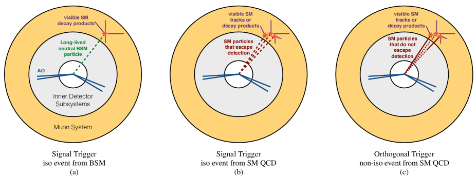
Figure 1: Schematic representation of signal and background events that pass the signal and orthogonal triggers. Dashed lines indicate invisible or undetected particles. All regular detector objects (prompt leptons, jets, etc.) that are produced in association with the LLP(s) are referred to as Associated Objects (AOs).

Henceforth we refer to events that pass the iso trigger and have a reconstructed displaced vertex as events in the iso-region (or iso-events), and events that pass the non-iso trigger and do not pass isolation criteria with a reconstructed displaced vertex as events in the non-iso-region (or non-iso-events). Because events that pass the non-iso trigger are SM-dominated, the non-iso trigger rate will be significantly larger than the rate of the isolated trigger, ensuring a suitably large control sample for estimating the number of expected iso-region events due to SM backgrounds . Specifically,

$$\frac{d\sigma^{SM}_{\mathrm{iso}}}{dx_{1}dx_{2}\ldots}\ \ \approx\ \ \frac{d\sigma_{\mathrm{non\mathchar 45\relax iso}}}{dx_{1}dx_{2}\ldots}\ \cdot\ r_{\mathrm{non\mathchar 45\relax iso\to iso}}(x_{1},x_{2},\ldots)$$ (3)

and the rescaling function $r_{\mathrm{non\mathchar 45\relax iso\to iso}}$ is related to the ratio of probabilities $\epsilon^{\mathrm{fake}}_{\mathrm{iso}}/\epsilon^{\mathrm{fake}}_{\mathrm{non\mathchar 45\relax iso}}$, where $\epsilon^{\mathrm{fake}}_{\mathrm{non\mathchar 45\relax iso}}$ is the probability for a QCD jet (or other SM event) to fire the non-iso orthogonal trigger.

The differential rescaling function $r_{\mathrm{non\mathchar 45\relax iso\to iso}}$ allows us to obtain a prediction of the SM background events in the iso-region event sample by using the non-iso-region events. The differential determination of $r_{\mathrm{non\mathchar 45\relax iso\to iso}}$ is important for enabling the imposition of additional cuts. For example, when requiring a high-$p_{T}$ jet and/or an isolated lepton in the iso-region event sample, we can obtain a background prediction by applying the same criteria to the non-iso-region events and rescaling.

II.1 Determining the rescaling function

The function $r_{\mathrm{non\mathchar 45\relax iso\to iso}}$ needs to be measured from data. This can be achieved by identifying some variable $Y$ (e.g., the number of identified leptons, or the angle between the MET vector and the displaced vertex) that fulfills two requirements:

1. for fixed $x_{i}$, the rescaling function $r_{\mathrm{non\mathchar 45\relax iso\to iso}}$ is independent of $Y$, and

2. $Y$ can be used to split the iso and non-iso-events into a signal-like region SR_Y, and a control-like region CR_Y. SR_Y contains the BSM signal of interest while CR_Y is by comparison SM-enriched.

The separation of the iso-region and non-iso-region events into SR_Y and CR_Y by using the variable $Y$ results in one signal region A and three control regions B,C,D as shown schematically in Fig. 2. The BSM signal events dominantly populate region A. As noted above, by design $r_{\mathrm{non\mathchar 45\relax iso\to iso}}$ is the same in SR_Y as in CR_Y and consequently can be determined from data in regions C and D,

$$r_{\mathrm{non\mathchar 45\relax iso\to iso}}(x_{1},x_{2},\ldots)\ \equiv\ \frac{d\sigma_{\mathrm{C}}^{\mathrm{data}}}{dx_{1}dx_{2}\ldots}\ \cdot\ \left[\frac{d\sigma_{\mathrm{D}}^{\mathrm{data}}}{dx_{1}dx_{2}\ldots}\right]^{-1}\ ,$$ (4)

thus making it possible to obtain a background prediction for region A:

$$\frac{d\sigma_{\mathrm{A}}^{\mathrm{prediction}}}{dx_{1}dx_{2}\ldots}\ \ =\ \ \frac{d\sigma_{\mathrm{B}}^{\mathrm{data}}}{dx_{1}dx_{2}\ldots}\ \cdot\ r_{\mathrm{non\mathchar 45\relax iso\to iso}}(x_{1},x_{2},\ldots).$$ (5)

Having the background prediction enables a search for BSM signals with just one DV in the Muon Spectrometer.

Figure 2: Schematic representation of the four regions A, B, C, D into which the iso-region and the non-iso-region events are divided. By construction, region A is significantly enriched with BSM signal events compared to region C.

There is the practical question of how to parametrize the function $r_{\mathrm{non\mathchar 45\relax iso\to iso}}$. The SM contribution to both the iso-region and non-iso-region is dominated by events where a single jet reconstructs a vertex in the MS. Both the probability that a jet will reconstruct a vertex in the MS and the probability that the vertex will pass isolation criteria depend on the local properties of the jet itself. Thus we expect $r_{\mathrm{non\mathchar 45\relax iso\to iso}}$ to be a function of the jet’s $p_{T}$ and $\eta$ (assuming azimuthal symmetry). In general we would expect the $\eta$ dependence to be non-negligible, resulting in, e.g., different values of $r_{\mathrm{non\mathchar 45\relax iso\to iso}}$ in the barrel and in the endcaps. For our present purposes, we approximate $r_{\mathrm{non\mathchar 45\relax iso\to iso}}$ as independent of $\eta$ for simplicity, and focus on what we expect to be the most important kinematic dependence, the jet $p_{T}$. Given that an energy measurement of the jet that fakes the DV is not available (by definition, especially in the iso-region), we hypothesize that the kinematic dependence of $r_{\mathrm{non\mathchar 45\relax iso\to iso}}$, to the extent that it exists, can be captured mostly as a function of the variable $H_{T}^{\prime}$,

$$H_{T}^{\prime}\equiv\left(\sum_{i}|\vec{p}_{T\,i}^{\ (AO)}|\right)+\mathrm{MET}^{\prime}$$ (6)

where $\vec{p}_{T\,i}^{\ (AO)}$ are the transverse momenta of the associated objects (regular prompt leptons, jets, etc.) and

$$\mathrm{MET}^{\prime}=|\vec{E}_{T}^{\ \prime\,\mathrm{miss}}|,\phantom{move}\vec{E}_{T}^{\ \prime\,\mathrm{miss}}\equiv-\sum_{i}\vec{p}_{T\,i}^{\ (AO)}.$$ (7)

Note that $\vec{E}_{T}^{\ \prime\,\mathrm{miss}}$ is just the regular transverse missing energy 2-vector for iso-events, but for non-iso events, jets between the interaction point and the Muon RoI are treated as invisible to ensure the variable definitions are equivalent for iso- and non-iso-region events. We therefore assume for this paper that $r_{\mathrm{non\mathchar 45\relax iso\to iso}}\approx r_{\mathrm{non\mathchar 45\relax iso\to iso}}(H_{T}^{\prime})$. In practice, an experimental analysis adopting this approach will need to determine the most useful parameterization .

In any analysis it will be important to assess both the applicability of this background estimation technique and the systematic uncertainty in the experimental determination of the function $r_{\mathrm{non\mathchar 45\relax iso\to iso}}$. This can be done by further subdividing CR_Y and checking for consistency of Eq. (5). In addition, when splitting both iso- and non-iso-region events into SR_Y and CR_Y using the kinematic variable $Y$, care has to be taken that events in control region C populate the same range of relevant kinematic variables (e.g., $H_{T}^{\prime}$) as BSM events in the signal region A.

II.2 Statistical Uncertainties and Cuts

As usual, the uncertainty of the resulting data-driven prediction for the background is limited by the statistical uncertainty in the control regions. We now discuss the statistical precision available for a background estimate given a choice of signal and control regions, first by ignoring non-$Y$ kinematic dependencies for simplicity, and then extending the discussion to the case of interest where signal and control regions are considered differentially in $H_{T}^{\prime}$.

The first task is to choose the kinematic variable $Y$, defining the signal-like and control-like regions of Fig. 2. The number of iso BSM and SM events in SR_Y and CR_Y must satisfy

$$\frac{N_{\mathrm{C}}^{\mathrm{BSM}}}{N_{\mathrm{A}}^{\mathrm{BSM}}}<\frac{N_{\mathrm{C}}^{\mathrm{SM}}}{N_{\mathrm{A}}^{\mathrm{SM}}}\ .$$ (8)

Ideally, the inequality is actually $\ll$, but in either case one might have to deal with BSM contamination of CR_Y, which we will discuss below. Because $r_{\mathrm{non\mathchar 45\relax iso\to iso}}$ is by assumption the same in SR_Y and CR_Y, and the non-iso-events are highly SM-dominated, we can write this condition as

$$\frac{N_{\mathrm{C}}^{\mathrm{BSM}}}{N_{\mathrm{A}}^{\mathrm{BSM}}}<\frac{N_{\mathrm{D}}}{N_{\mathrm{B}}}\ ,$$ (9)

where the LHS can be computed from the Monte Carlo signal prediction, and the RHS is determined purely from data.

Note that satisfying Eq. (9) does not imply that $N_{\mathrm{D}}>N_{\mathrm{B}}$, or equivalently $N_{\mathrm{C}}^{\mathrm{SM}}>N_{\mathrm{A}}^{\mathrm{SM}}$. It merely requires that CR_Y contain a larger fraction of iso SM events than SR_Y. Ignoring kinematic dependence,

$$r_{\mathrm{non\mathchar 45\relax iso\to iso}}=\frac{N_{C}}{N_{D}},$$ (10)

with relative uncertainty

$$\frac{\delta r_{\mathrm{non\mathchar 45\relax iso\to iso}}}{r_{\mathrm{non\mathchar 45\relax iso\to iso}}}=\frac{1}{\sqrt{N_{C}}}\ .$$ (11)

(For simplicity, we here ignore contamination from BSM events in the various control regions, ignore systematic uncertainties in the determination of $r_{\mathrm{non\mathchar 45\relax iso\to iso}}$, and assume that all event numbers are sufficiently large that the Poisson fluctuation for $N$ events is simply $\sqrt{N}$. We also ignore the subdominant contribution to $\delta r_{\mathrm{non\mathchar 45\relax iso\to iso}}$ from the statistical uncertainty in region D, since the non-iso-region is much more populated than the iso-region.) This gives the expected number of background events in region A,

$$\langle N_{A}^{\mathrm{SM}}\rangle\ \ =\ \ r_{\mathrm{non\mathchar 45\relax iso\to iso}}\,N_{B}\ \ =\ \ \frac{N_{C}}{N_{D}}\,N_{B}.$$ (12)

Therefore, if the ideal scenario of $N_{\mathrm{D}}\gg N_{\mathrm{B}}$ is realized (keeping in mind that $N_{B}\gg N_{A}$ and $N_{D}\gg N_{C}$), the 95% CL limit on the number of BSM events in region $A$ is approximately

$$N_{A}^{\mathrm{BSM}}\ \ <\ \ 2\sqrt{N_{A}^{\mathrm{SM}}}\ ,$$ (13)

which is determined by the Poisson fluctuations of the SM background in region A, with no significant added uncertainty from $r_{\mathrm{non\mathchar 45\relax iso\to iso}}$. If, conversely, CR_Y is not as populated as SR_Y, i.e., $N_{\mathrm{D}}\ll N_{\mathrm{B}}$ and hence $N_{\mathrm{C}}^{\mathrm{SM}}\ll N_{\mathrm{A}}^{\mathrm{SM}}$, then the rescaling uncertainty in Eq. (11) is much larger than the Poisson fluctuations of the SM background in signal region A. Therefore, the 95% CL limit on the number of BSM events in region $A$ is approximately

$$N_{A}^{\mathrm{BSM}}\ \ <\ \ 2\sqrt{N_{A}^{\mathrm{SM}}}\ \sqrt{\frac{N_{B}}{N_{D}}}\ .$$ (14)

The sensitivity is degraded by the square root of the factor by which CR_Y has worse statistics than SR_Y.

We now restore the kinematic dependence to make explicit how cuts on kinematic variables are performed. Since we parameterize $r_{\mathrm{non\mathchar 45\relax iso\to iso}}$ as a function of $H_{T}^{\prime}$, we will treat all events, whether simulated, predicted, or from data, as binned in $H_{T}^{\prime}$, with bins $H_{T,i}^{\prime}$ and bin occupations $N_{i}$.

All of the above expressions apply in each $H_{T}^{\prime}$ bin, i.e., taking $N\to N_{i}$, etc. So, for example, the rescaling function is defined bin-by-bin as

$$r_{\mathrm{non\mathchar 45\relax iso\to iso}}(H_{T,i}^{\prime})=r_{\mathrm{non\mathchar 45\relax iso\to iso}}^{i}=\frac{N_{C,i}}{N_{D,i}},$$ (15)

with relative uncertainty

$$\frac{\delta r_{\mathrm{non\mathchar 45\relax iso\to iso}}^{i}}{r_{\mathrm{non\mathchar 45\relax iso\to iso}}^{i}}=\frac{1}{\sqrt{N_{C,i}}}\ .$$ (16)

The background prediction in region A is given by

$$\langle N_{A,i}^{\mathrm{SM}}\rangle\ \ =\ \ \left(\frac{N_{B,i}}{N_{D,i}}\right)\,N_{C,i},$$ (17)

where the statistical uncertainty of $N_{C,i}$ dominates the uncertainty of $\langle N_{A,i}^{\mathrm{SM}}\rangle$. In particular, if no events are observed in a control region C bin, $N_{C,i}=0$, then we only have an upper bound on $\langle N_{A,i}^{\mathrm{SM}}\rangle$. To perform cuts on the events in region $A$, the corresponding SM prediction after cuts can be obtained by performing those cuts on the non-iso-events:

$$\langle N_{A,i}^{\mathrm{SM,\ after\ cuts}}\rangle\ \ =\ \ \left(\frac{N_{B,i}^{\mathrm{after\ cuts}}}{N_{D,i}}\right)\,N_{C,i}$$ (18)

The corresponding predictions $N_{A,i}^{\mathrm{BSM}}$ or $N_{A,i}^{\mathrm{BSM,\ after\ cuts}}$ for the signal can be obtained from Monte Carlo.

II.3 Important Considerations

The best choice of the observable $Y$ used to define CR_Y and SR_Y will depend on the signal model. Choosing a CR_Y is very easy if, for example, the LLPs are always or frequently produced in association with certain specific AOs, such as a lepton. In that case, a good CR_Y would simply invert the lepton requirement, ensuring very large CR_Y statistics, and thereby allowing the CR_Y sample to be subdivided to further reduce systematic uncertainties. By contrast, when the LLPs are dominantly produced with few or no AOs, as occurs for exotic Higgs decays to LLPs, choosing a CR_Y becomes more challenging. We discuss this in greater detail in the next Section.

As discussed above, one of the requirements that $Y$ must satisfy is that $r_{\mathrm{non\mathchar 45\relax iso\to iso}}(H_{T}^{\prime})$ is independent of $Y$ for fixed values of $H_{T}^{\prime}$. When dealing with a binned rescaling function $r_{\mathrm{non\mathchar 45\relax iso\to iso}}^{i}$, Eq. (15), this becomes the requirement that, in a given $H_{T}^{\prime}$ bin, $r_{\mathrm{non\mathchar 45\relax iso\to iso}}(H_{T}^{\prime})$ is a sufficiently slowly varying function that any correlations of $Y$ with $H_{T}^{\prime}$, and therefore any differences of $r_{\mathrm{non\mathchar 45\relax iso\to iso}}^{i}$ between SR_Y and CR_Y, are negligible. A violation of this requirement would introduce a systematic uncertainty in an individual bin’s background prediction in region A that, unlike the statistical uncertainties discussed above, does not scale with luminosity. Fortunately, since increased statistics allow for smaller bin sizes, the overall effect of this systematic error on the search sensitivity will actually decrease with luminosity. As outlined below, we therefore expect weak correlations to be manageable in a real analysis.

To quantify how slowly varying $r_{\mathrm{non\mathchar 45\relax iso\to iso}}$ needs to be in order for this systematic error to be negligible, consider a single $H_{T}^{\prime}$ bin $(H_{T,1}^{\prime},H_{T,2}^{\prime})$ with bin occupation $N_{C}$ in region C, and similarly for region A. Define

$$\Delta H_{T}^{\prime}=\frac{|\langle H_{T}^{\prime}\rangle_{C}-\langle H_{T}^{\prime}\rangle_{A}|}{H_{T,2}^{\prime}-H_{T,1}^{\prime}}<1\ ,$$ (19)

which is the difference, between region A and region C, of the mean $H_{T}^{\prime}$ in this bin, normalized to the bin width. The limit of no correlations between $H_{T}^{\prime}$ and $Y$ corresponds to $\Delta H_{T}^{\prime}\to 0$. Assuming the bin is narrow enough that $r_{\mathrm{non\mathchar 45\relax iso\to iso}}(H_{T}^{\prime})$ is approximately linear across the bin, the condition that the systematic error in $r_{\mathrm{non\mathchar 45\relax iso\to iso}}$ is negligible compared to its statistical uncertainty can then be written as

$$\frac{|r_{\mathrm{non\mathchar 45\relax iso\to iso}}(H_{T,2}^{\prime})-r_{\mathrm{non\mathchar 45\relax iso\to iso}}(H_{T,1}^{\prime})|}{r_{\mathrm{non\mathchar 45\relax iso\to iso}}(H_{T}^{\prime})}\ll\frac{1}{\sqrt{N_{C}}\ \Delta H_{T}^{\prime}},$$

(20)

where the denominator on the LHS is the average value of $r_{\mathrm{non\mathchar 45\relax iso\to iso}}$ in this bin. (Note that this condition is trivially satisfied if there are no correlations between $H_{T}^{\prime}$ and $Y$.) In the limit of large statistics, both $\Delta H_{T}^{\prime}$ and $r_{\mathrm{non\mathchar 45\relax iso\to iso}}(H_{T}^{\prime})$ are approximately invariant with bin-size. On the other hand, the numerator on the LHS and $N_{C}$ decrease if we shrink the bin. In optimizing a given analysis, we can therefore hope to satisfy this condition by choosing the smallest possible bin size that still ensures each bin in region C is populated with at least a few events . In that case one expects $\Delta H_{T}^{\prime}\gtrsim\mathcal{O}(0.1)$ purely due to random scatter. In order for systematic error to be significant and Eq. (20) to be violated, $r_{\mathrm{non\mathchar 45\relax iso\to iso}}(H_{T}^{\prime})$ would have to vary by at least an $\mathcal{O}(1)$ factor across a single $H_{T}^{\prime}$ bin. Whether this is the case depends on the statistics in $CR_{Y}$, but based on our toy analysis of a single DV in the MS in Section III, we expect this effect to be negligible or controllable in a real analysis. Furthermore, the need to contend with weak correlations when using the ABCD method is a familiar issue. For example, the ABCD analysis of Ref. Aad et al. (2016) obtains good results in the presence of correlations of typically 6%–10% between their control variables, which are handled by marginalizing over nuisance parameters in a likelihood function.

One may also have to contend with BSM contamination of the control region. We will account for this in our estimate in Sec. III by including BSM contributions in $N_{C}$, but we will underestimate the strength of the obtainable exclusions by not using that knowledge when deriving a limit on the number of BSM events in region $A$. In a fully self-consistent analysis, a given hypothesis for the BSM cross-section could be tested by subtracting the (known) BSM contribution from the measured $N_{A}$ and $N_{B}$, then deriving $r_{\mathrm{\mathrm{non\mathchar 45\relax iso\to iso}}}(H_{T}^{\prime})$ in both SR_Y and CR_Y and checking for inconsistencies, which may arise if significant amounts of BSM signal are present that, by construction, populate SR_Y and CR_Y in different proportions. (We discuss more model-independent approaches in Section IV.)

We now demonstrate this data-driven technique by computing a toy sensitivity estimate for a simple and well-motivated benchmark signal model in Section III. This will clarify many of the practical details of how such an analysis would be performed. In Section IV, we discuss generalizations for other signal models, and LLP searches in other detector subsystems.

III Example: $h\to XX$ analysis

In this section we demonstrate how the background estimation strategy of Section II is applied in practice. The signal we consider is the production of a scalar $\Phi$ via gluon fusion, followed by its decay to two identical unstable particles $X$. Such decays are among the leading signatures of, for example, theories of Neutral Naturalness or Hidden Valleys where the decaying scalar is the 125 GeV SM-like Higgs boson. As we discuss below, this signal model is also one of the most challenging for which to implement our analysis strategy, since the inclusive production mode of the LLPs prohibits the most obvious choices of $Y$ to define a SR_Y/CR_Y split. Even so, we show in a toy model estimate that significant sensitivity gains at long proper lifetimes are possible compared to a search for two DVs in the MS ATLAS Collaboration (2015a).

We assume the $X$ decays to pairs of SM particles via a small mixing with the SM-like Higgs. The parameters of the signal model are therefore:

• $\sigma_{\Phi}\cdot\mathrm{Br}(\Phi\to XX)\equiv\sigma_{\Phi\to XX}$

• $m_{\Phi}$

• $m_{X}<m_{\phi}/2$

• $c\tau_{X}$

For simplicity we assume $\Phi$ has a narrow decay width. The sensitivity of a search is quantified as the value of $\sigma_{\Phi\to XX}$ that can be excluded for a given $(m_{\Phi},m_{X},c\tau_{X})$. Since exotic decays of the SM-like 125 GeV Higgs boson are particularly well-motivated Curtin et al. (2014), we set $\Phi=h$ and hence $m_{\Phi}=m_{h}$ in our estimate, but the analysis generalizes easily to other cases.

III.1 Control regions for $h\to XX$

The particular challenge posed by the $h\to XX$ signal model is the lack of any distinctive AOs produced in association with the LLPs. Thus, the non-iso sample that is most closely related to the iso sample of interest is the entire inclusive sample. Defining a separate control region that includes an AO, for instance an identified lepton, would indeed define three control and one signal region as shown Fig. 2. However, the small statistics of CR_Y and resulting large uncertainty on the region A background prediction, $N_{B}/N_{D}$, would typically be so large that no useful limit can be extracted. The best one could do by requiring an AO, from the point of view of relative event rates, is to define a CR_Y that requires a single $b$-tag. In this case the resulting signal and control regions do not satisfy Eq. (9), because, taking the $p_{T}$-dependence of realistic $b$-tagging algorithms into account, both BSM and SM processes include contributions of similar relative size with associated tagged $b$-jets. Fortunately, this signal model pair-produces LLPs, and the LLP that is not reconstructed as a DV can be used to inform choices for the variable $Y$, which depend on the LLP lifetime.

We will focus here on long lifetimes of $X$, since this is the regime where a single-DV search in the MS has unique sensitivity compared to other displaced searches. In this case, events with one DV will typically feature one $X$ decaying in the MS, while the other $X$ escapes the detector. The MET in signal events is then sensitive to the Higgs $p_{T}$, which is typically only of order tens of GeV. Given that the typical MET resolution is $\mathcal{O}(10\;\mathrm{GeV})$ ATLAS Collaboration (2015d), the MET vector in signal events will be highly sensitive to soft jet and pileup activity, and not preferentially aligned with the DV. The dominant SM background is dijet production, with one jet faking a DV. In these events, there is no source of ‘truth-level’ MET aside from the energy of the mis-measured jet. Since harder jets are expected to be more likely to reach the MS and fake a DV, the MET is expected to be peaked at higher values than for BSM events, and will preferentially point along the DV. Therefore, the angle in the transverse plane $\Delta\phi(\mathrm{MET},\mathrm{DV})$ between the DV in the Muon Spectrometer and the missing transverse energy 2-vector is a useful choice for the variable $Y$. This variable is also suitable because it is not strongly correlated with the fake jet energy, and therefore with $H_{T}^{\prime}$. A CR_Y can be defined by the requirement $\Delta\phi(\mathrm{MET},\mathrm{DV})<\Delta\phi_{min}$.

For shorter $X$ proper lifetimes, $c\tau\lesssim\mathcal{O}(1)$ m, such an analysis is obviously not optimal, because the $X$ that does not decay in the MS is now most likely to decay in one of the other detector systems closer to the IP, causing the MET to again be aligned with the DV. In this regime, the best choice of variable to split SR_Y from CR_Y is likely to be some unusual property of objects in the tracker or calorimeters. In order for one $X$ to reach the muon system, even with high luminosity to allow access to the tail of the boost distribution, its lifetime must be more than a few centimeters. With such proper lifetimes, the $X$ decaying in the other detector systems will have signatures such as trackless jets and/or displaced vertices in the inner tracker. This offers a control region given by a veto on unusual objects in the inner detector, such as only allowing events where each AO passes a stringent quality cut to ensure it originates at the primary vertex, and thus lead to greater signal acceptance than would be obtained by requiring the identification and reconstruction of a second displaced vertex. We expect that this strategy would significantly enhance the sensitivity of a search for a single DV in the MS for short $X$ proper lifetimes. However, explicitly modeling the impact of such vetos with publicly available tools is difficult to do with any quantitative reliability, and since the unique advantage of the MS search is the long-lifetime regime, we will not discuss this short-lifetime case in detail.

III.2 Toy Sensitivity Estimate

We now perform a Monte Carlo study to compute the potential sensitivity of our analysis strategy. This has to be regarded as a toy estimate, since the difficulty of accurately simulating SM contributions that fake DVs was the very motivation for developing our data-driven background estimation. QCD background will be estimated in two ways: one that is more optimistic, and one that is extremely pessimistic. As explained below, we expect that the optimistic estimate is the more realistic of the two, but we show results for both possibilities, since they are likely to bracket the achievable sensitivity. The obtained limit projections differ only by an $\mathcal{O}(1)$ factor, which gives us confidence that these rough estimates are robust within their understood precision. In each case, we expect significant improvements compared to the background-free search for 2 DVs in the MS.

III.2.1 Computation of BSM contributions

Concentrating on the case where $\Phi=h$ is the SM-like Higgs, we normalize the inclusive Higgs production cross-section to the value computed by the LHC Higgs Cross-Section Working Group Andersen et al. (2013) and parametrize limits as reach projections of $\mathrm{Br}(h\to XX)$, assuming SM production. The Hidden Abelian Higgs Model (HAHM) Curtin et al. (2015) is used to generate gluon-fusion $h\to XX$ events in Madgraph Alwall et al. (2014), with matched production of up to one extra jet, that are showered and hadronized in Pythia 6 Sjostrand et al. (2008) .

The probability that each signal event passes the trigger and yields a reconstructed DV in the MS can be estimated by calculating the probability of decaying within the sensitive regions of the MS, see Table 1, for a given lifetime, and convolving with trigger and DV reconstruction efficiencies ATLAS Collaboration (2015a), where we ignore an $\mathcal{O}(1)$ $m_{X}$-dependence of that efficiency for the purpose of this simple estimate.

	$r$ (m)	$|z|$ (m)	$|\eta|$	$\epsilon_{\mathrm{trigger}}$	$\epsilon_{\mathrm{DV}}$
Muon Spectrometer (barrel)	(4, 6.5)	—	$<1.1$	0.40	0.25
Muon Spectrometer (endcaps)	—	(7, 12)	(1.1, 2.4)	0.25	0.50

Table 1: Regions of the ATLAS Muon Spectrometer that have sensitivity to LLP decays. We assume uncorrelated efficiencies $\epsilon_{\mathrm{trigger}}$ and $\epsilon_{\mathrm{DV}}$ for an LLP decaying in the given detector region to pass the Muon RoI Signal trigger and be reconstructed as a DV offline, respectively. For simplicity we ignore a modest dependence on $m_{X}$. The geometrical definition of sensitive detector regions and approximate trigger/reconstruction efficiencies for displaced $h\to XX\to 4f$ decays are taken from efficiency curves in ATLAS Collaboration (2015a).

Due to the unusual nature of our signal we do not use any detector simulation, but manually include relevant detector effects by analyzing Pythia-clustered, truth-level events. For each event:

• Any $X$ that decays before reaching the Muon Spectrometer is treated as a regular jet.

• Jets $j_{i}$, ordered by $p_{T}$, are counted if they have $p_{T}^{j_{i}}>20\;\mathrm{GeV}$ and $|\eta|<2.4$.

• The above set of jets determines the two-vector $\vec{E}_{T}^{miss}=-\sum_{i}\vec{p}_{T}^{j_{i}}$. The most important detector effect to include is the resolution on both the size and direction of this vector.

  To accurately model the MET resolution, we need to take into account the effects of pile-up. For each event, we choose a number $N_{PV}$ of primary vertices. This is done as follows:

  • For $\sqrt{s}=8\;\mathrm{TeV}$, we use the LHC Run-1 distribution ATLAS Collaboration (2012b) of the mean number of interactions per crossing $\langle\mu\rangle$, which is 20.7 on average. The resulting number of primary vertices can be obtained from the parameterization

    $$\langle N_{PV}\rangle=0.73\langle\mu\rangle(1-0.008\langle\mu\rangle)$$ (21)

    in Ref. ATLAS Collaboration (2015e), which results in a distribution of expected $\langle N_{PV}\rangle$ that is peaked around 17. That $\langle N_{PV}\rangle$ distribution is sampled to obtain an expected $\langle N_{PV}\rangle$ for each event, which in turn defines a Poisson distribution that is sampled to obtain the observed $N_{PV}$ for that event.

  • For $\sqrt{s}=13\;\mathrm{TeV}$ with $30{\ \rm fb}^{-1}$ or $300{\ \rm fb}^{-1}$, we use the 13 TeV $\langle\mu\rangle$ distribution given in Ref. ATLAS Collaboration (2015f), which has an average of 13.5. Since that distribution was obtained from a low-luminosity run, we shift it upwards by doubling $\langle\mu\rangle$ (without increasing the width of the curve) to more realistically model the higher pile-up conditions of the full LHC run 2. Using the $\langle\mu\rangle$-distribution thus defined, we follow the same steps as for $8\;\mathrm{TeV}$.

  • For $\sqrt{s}=13\;\mathrm{TeV}$ with $3000{\ \rm fb}^{-1}$, ATLAS Collaboration (2014c) shows explicit distributions of $N_{PV}$ for different assumptions of $\langle\mu\rangle$. We choose the curve with an average $\langle\mu\rangle$ of $140$ scenario as our benchmark point, and sample that curve directly to obtain $N_{PV}$ for each event.

  Ref. ATLAS Collaboration (2015d) contains Track-based soft term (TST) MET resolution curves as a function of $N_{PV}$. For each event, the chosen $N_{PV}$ defines an RMS uncertainty (typically about $\ 10-20\;\mathrm{GeV}$) for each $(E_{T}^{miss})_{x,y}$ component. This in turn defines the variance of a Gaussian distribution that is again sampled to generate the spurious $(E_{T}^{miss})_{x,y}$ components, which are added to the truth-level $\vec{E}_{T}^{miss}$.

• $\vec{E}_{T}^{miss}$ is used to compute $\Delta\phi(\mathrm{MET},\mathrm{DV})$, as well as $\mathrm{MET}=|\vec{E}_{T}^{miss}|$.

  Note that, for small values of MET, the finite MET resolution means that the angle $\Delta\phi(\mathrm{MET},\mathrm{DV})$ is largely unrelated to its value at truth level, while for large MET values $\Delta\phi(\mathrm{MET},\mathrm{DV})$ will be peaked at its truth-level value. As explained above, we exploit this in our analysis.

• $H_{T}^{\prime}$ is computed as in Eq. (6) using the AOs, i.e., the above-defined jets $j_{i}$ and $\vec{E}_{T}^{miss}$.

Since $\Delta\phi(\mathrm{MET},\mathrm{DV})$ will be used to define SR_Y and CR_Y, the above variables will allow BSM predictions to be computed in regions A and C of Fig. 2, i.e., in the iso-regions. We have checked that our results are robust under different modeling of the MET resolution.

Note that we were very careful to model experimental resolution for MET-related quantities, because $\Delta\phi(\mathrm{MET},\mathrm{DV})$ is vital for the definition of our signal and control regions, but we did not account for detector effects in the computation of $p_{T}^{j_{i}}$ and therefore in $H_{T}^{\prime}$. This is acceptable for our toy estimate, since whenever we make use of these variables we only exploit the coarse structure of their distributions. Fine details in these distributions, arising from finite jet energy resolution, do not affect our results. We also assume that trigger efficiencies remain constant at high luminosities.

III.2.2 Computation of SM Contributions

QCD contributions to the iso- and non-iso-regions are very difficult to model reliably—this is exactly the reason why a data-driven approach is necessary. Even so, we can perform some estimates of the QCD contributions that are sufficient to demonstrate that our analysis strategy will improve sensitivity to very long-lived BSM particles.

For estimating sensitivity, the two most important questions are:

1. What is the size of the SM contribution in the signal region A?

2. What is the precision with which the SM contribution in region A can be determined from data?

Answering both of these questions only requires simulating events in the iso-region. This can be easily seen by rewriting Eq. (18) for the data-driven prediction of the SM contribution in region A:

$$\langle N_{A,i}^{\mathrm{SM,\ after\ cuts}}\rangle = \left(\frac{N_{B,i}^{\mathrm{after\ cuts}}}{N_{D,i}}\right)\,N_{C,i}$$

$$= \ \ \left(\frac{N_{A,i}^{\mathrm{SM_{\mathrm{MC}},after\ cuts}}}{N_{C,i}^{\mathrm{SM_{\mathrm{MC}}}}}\right)\,N_{C,i}^{\mathrm{SM_{\mathrm{MC}}+BSM_{\mathrm{MC}}}}\ ,$$

where the MC subscript indicates the quantity is computed from Monte Carlo. The second equality occurs because the kinematic variable $Y$ in Fig. 2 is assumed to be uncorrelated with the isolation condition, and $N_{C,i}=N_{C,i}^{\mathrm{SM_{\mathrm{MC}}+BSM_{\mathrm{MC}}}}$ simply reflects the fact that we are simulating events in the iso-region . This conservative estimate of $\langle N_{A,i}^{SM}\rangle$ does not account for signal contamination in control-like regions. The quantity in brackets can be assumed to be known to extremely high precision, because of the much higher statistics in the non-iso-region than in the iso-region (even though we use a ratio of quantities computed from Monte Carlo in the iso-region to describe it for our sensitivity estimate). For finite statistics in iso-regions A and C, the dominant contribution to the uncertainty of $\langle N_{A,i}^{\mathrm{SM,\ after\ cuts}}\rangle$ is the statistical uncertainty of $N_{C,i}^{\mathrm{SM_{\mathrm{MC}}+BSM_{\mathrm{MC}}}}$. For the purpose of our sensitivity estimate, we can therefore define

$$\langle N_{A,i}^{\mathrm{SM,\ after\ cuts}}\rangle\ \ =\ \ \left(\frac{N_{A,i}^{\mathrm{SM_{\mathrm{MC}},after\ cuts}}}{N_{C,i}^{\mathrm{SM_{\mathrm{MC}}}}}\right)\,(\tilde{N}_{i})^{+\delta_{+i}}_{-\delta_{-i}}\ ,$$ (23)

where $\tilde{N}_{i}$ is the number of events we observe in $H_{T}^{\prime}$ bin $i$ of region C, and $\delta_{\pm i}$ are the Poisson uncertainties for the observation of $\tilde{N}_{i}$ events. We will take $\tilde{N}_{i}$ to be given $N_{C,i}^{\mathrm{SM_{\mathrm{MC}}+BSM_{\mathrm{MC}}}}$ rounded up to the nearest integer, which is a conservative choice.

We now discuss how to simulate QCD jets generating DVs in the Muon Spectrometer. The ATLAS Run-1 analysis ATLAS Collaboration (2015a) observed about $1.0\times 10^{5}$ events that fired the Muon RoI Signal trigger. The chance that one of those events, which are assumed to stem dominantly from QCD, also results in a reconstructed DV in the corresponding Muon RoI is about $1.3\times 10^{-2}$ in the MS Barrel and $8.0\times 10^{-2}$ in the endcaps. The numbers of events that both fired the trigger and reconstructed a DV in the barrel versus in the endcaps are not separately given. Consequently the total number of QCD events with a single reconstructed DV in the ATLAS MS in Run-1 could range between $\sim 1300$ for all vertices in the barrel, and $~{}8000$ for all vertices in the endcaps. We take as our estimate the total number to be $\sim 3000$. This will at most be off by a factor of $\sim 3$ from the real value in either direction, which will not significantly affect our conclusions. We therefore assume that, at truth level,

$$\sum_{i}N_{A,i}^{\mathrm{SM}}=3000$$ (24)

for $\sqrt{s}=8\;\mathrm{TeV}$ with $25{\ \rm fb}^{-1}$, where the sum is over all $H_{T}^{\prime}$ bins. For simplicity, we assume the cross-section to produce fake DVs from QCD does not change significantly between $\sqrt{s}=7\;\mathrm{TeV}$ and 8 TeV. The ATLAS analysis also estimated the number of QCD background events in the signal region of their search, which required two displaced vertices in the MS. It was found to be

$$N_{\mathrm{2DV}}^{\mathrm{SM}}\sim\mathcal{O}(0.1),\ \ \ \ \ \ \ \ \mbox{for $\sqrt{s}=8\;\mathrm{TeV}$ with $25{\ \rm fb}^{-1}$}.$$ (25)

These two data points allow us to normalize our Monte Carlo prediction for generating fake DVs with QCD. To obtain concrete simulated events, we take an approach related to Eq. (2) and assume each jet has a $p_{T}$-dependent chance $\epsilon^{\mathrm{fake}}_{\mathrm{iso}}(p_{T})$ of faking a DV in the MS. For simplicity we assume $\epsilon^{\mathrm{fake}}_{\mathrm{iso}}(p_{T})$ to have a linear dependence,

$$\epsilon^{\mathrm{fake}}_{\mathrm{iso}}(p_{T})=\left\{\begin{array}[]{ll}\epsilon_{\mathrm{iso}}^{0}\times\displaystyle\frac{(p_{T}-p_{T}^{\mathrm{min}})}{\;\mathrm{GeV}}&\mbox{ for $p_{T}\geq p_{T}^{\mathrm{min}}$}\\ 0&\mbox{ for $p_{T}<p_{T}^{\mathrm{min}}$}\end{array}\right.\ ,$$ (26)

and consider two possibilities:

1. Optimistic choice: because we expect harder jets to be dominantly responsible for the DVs, a reasonable modeling of the QCD fake rate is to require a relatively large $p_{T}^{\mathrm{min}}$ that, along with $\epsilon_{\mathrm{iso}}^{0}$, is chosen to satisfy both Eqns. (24) and (25). With this assumption, the fake DV background is dominated by relatively energetic jets, allowing BSM and SM events to be effectively distinguished.

2. Pessimistic choice: assume that every jet is able to fake a DV in the MS by setting $p_{T}^{\mathrm{min}}=0\;\mathrm{GeV}$. The constant $\epsilon_{\mathrm{iso}}^{0}$ is then chosen to satisfy Eq. (24). This is a pessimistic choice for the shape of the SM background, because the fake DVs are dominated by very soft QCD jets with few kinematic features to distinguish them from Higgs production events with exotic decay to LLPs. Eq. (25) is also not satisfied, since the high production rate of soft jets means that $\epsilon_{\mathrm{iso}}^{0}$ is so small that $N_{\mathrm{2DV}}^{\mathrm{SM}}$ in Eq. (25) is predicted to be many orders of magnitude less than unity. We include this possibility in our analysis to demonstrate that even with these extremely pessimistic assumptions, our data-driven approach has more sensitivity at long lifetimes compared to a standard search requiring 2 DVs.

We will derive limit projections for both the pessimistic and the more realistic optimistic choice. The sensitivity of a real analysis will likely lie somewhere in between these possibilities.

Both QCD samples were simulated in MadGraph and showered and hadronized in Pythia 6. An unmatched dijet sample was used for the optimistic choice to adequately sample hard jets with $p_{T}>100\;\mathrm{GeV}$. Matched generation of 2 + 3 jets was used for the pessimistic choice to give sensible distributions of the soft jets. We use the tree-level QCD cross sections supplied by MadGraph, since any NLO effects are included in the normalization of the $\epsilon^{\mathrm{fake}}_{\mathrm{iso}}$ fake rate to Eqns. (24) and (25). This results in

$$\epsilon_{\mathrm{iso}}^{0} = 7.6\ \times\ 10^{-12}\ ,\ \ \ \ \ p_{T}^{\mathrm{min}}=0\;\mathrm{GeV}$$

for the pessimistic QCD scenario, and

$$\epsilon_{\mathrm{iso}}^{0} = 1.1\times 10^{-8}\ ,\ \ \ \ \ \ \ \ p_{T}^{\mathrm{min}}=120\;\mathrm{GeV}$$

for the optimistic  QCD  scenario, which also gives $N_{\mathrm{2DV}}^{\mathrm{SM}}\sim 0.1$.

In each QCD event, any jet with rapidity $|\eta|<2.4$ (so it can reach the MS) is considered as a possible fake DV, with the event weighted according to $\epsilon^{\mathrm{fake}}_{\mathrm{iso}}$. The remaining jets are used to reconstruct the event in an identical fashion as the signal events above.

We now discuss possible systematic errors in the data-driven determination of $r_{\mathrm{non\mathchar 45\relax iso\to iso}}$. As might be expected from the presence of additional energy scales in the event (e.g., from pile-up), some slight correlation between $H_{T}^{\prime}$ and $Y=\Delta\phi(\mathrm{MET},\mathrm{DV})$ is indeed present. Empirically, we determine $\Delta H_{T}^{\prime}$ in Eq. (19) to be $\lesssim 0.1$ for both our optimistic and pessimistic QCD background estimates. At the 13 TeV LHC with $30{\ \rm fb}^{-1}$, SM background rates are high enough that $H_{T}^{\prime}$ bins as narrow as 1 or 2 GeV are sufficiently populated in region C. Eq. (20) therefore implies that the systematic error is negligible unless $r_{\mathrm{non\mathchar 45\relax iso\to iso}}(H_{T}^{\prime})$ varies by a factor of about $5-10$ over an $H_{T}^{\prime}$ range of only a few GeV. Therefore, the systematic error should in general be negligible. However, as a consistency check, it should be verified that Eq. (20) is satisfied for the chosen binsize of a realistic analysis.

III.2.3 Analysis and Projected Limits: Search with Two Displaced Vertices

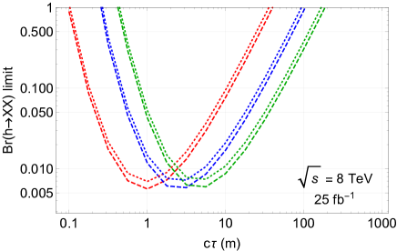
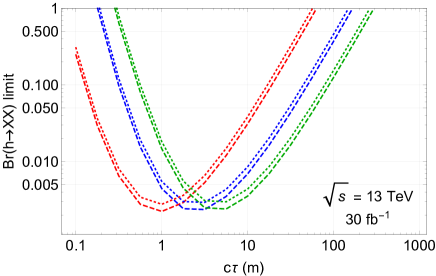
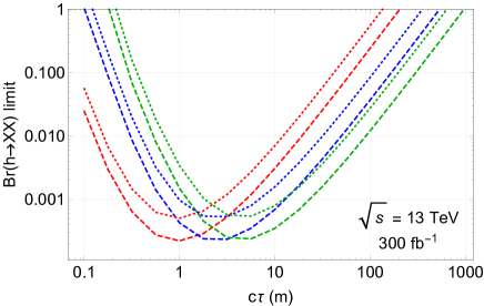
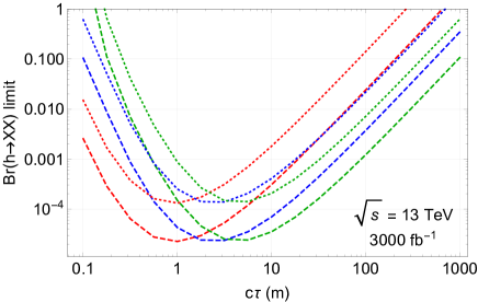
Figure 3: Simulated limits on $\mathrm{Br}(h\to XX)$ as a function of $X$ lifetime for $m_{X}=10,25,40\;\mathrm{GeV}$ at the 8 and 13 TeV LHC from a search that requires two DVs in the ATLAS Muon Spectrometer, in analogy to ATLAS Collaboration (2015a). This result serves as a baseline against which to compare our projections for a data-driven search requiring just a single DV.

We first derive estimated limits on $\mathrm{Br}(h\to XX)$ for an ATLAS search analogous to ATLAS Collaboration (2015a) that requires two DVs in the MS at the 13 TeV LHC. We also produce limit projections for $25{\ \rm fb}^{-1}$ of 8 TeV data to compare with ATLAS Collaboration (2015a) (even though we do not include the optional reconstruction of a second DV in the inner tracker instead of the MS). These limits for a search with two DVs will serve as a baseline against which we compare the sensitivity of our proposed data-driven search for a single DV.

These limit projections for the two-DV-search are derived under two assumptions. First, we show limits for zero background, which simply corresponds to about 4 signal events. Second, we show limits for non-zero background, derived by a naive rescaling of the LHC Run-1 background prediction in ATLAS Collaboration (2015a). At the 8 TeV LHC with $25{\ \rm fb}^{-1}$ this corresponds to 1 background event (rounded up from 0.4). At 13 TeV, this scales to about 1, 10 and 100 events respectively for $30{\ \rm fb}^{-1}$, $300{\ \rm fb}^{-1}$ and $3000{\ \rm fb}^{-1}$.

Once again, in a realistic search, the actual limits will lie somewhere between these two cases. However, since it is likely that improvements in DV reconstruction algorithms and other optimizations for higher luminosity will enable future analyses to suppress backgrounds to a greater extent than what is predicted by simply rescaling the results from Ref. ATLAS Collaboration (2015a), we will compare projected sensitivity of single-DV searches to the background-free two-DV limits. This also will give the most pessimistic assessment of the relative gained sensitivity of the one-DV search, and demonstrate the significance of these gains.

Our projected limits for the two-DV searches are shown in Fig. 3. The 8 TeV projections reproduce the actual limits of the ATLAS analysis ATLAS Collaboration (2015a) up to a $\mathcal{O}(1)$ factor. This modest difference is not surprising since we used a very simple parametrization of the DV reconstruction efficiency, which amongst other things neglected dependence on the LLP mass. Nevertheless, since our limits for a single DV are derived under the same assumptions, these sensitivities will serve as a valid base of comparison for the proposed one-DV search.

III.2.4 Analysis and Projected Limits: Search with One Displaced Vertex

Fig. 4 shows the distributions in $H_{T}^{\prime}$, $p_{T}^{j_{1}}$, MET and $\Delta\phi(\mathrm{MET},\mathrm{DV})$ of BSM and SM events in the iso-region at $\sqrt{s}=13\;\mathrm{TeV}$ before SR_Y and CR_Y are defined. This illustrates that while BSM events for long lifetimes are relatively uniformly distributed in $\Delta\phi(\mathrm{MET},\mathrm{DV})$, QCD events are peaked at $\Delta\phi(\mathrm{MET},\mathrm{DV})=0$, especially for the more optimistic QCD assumption of $p_{T}^{\mathrm{min}}=120\;\mathrm{GeV}$. We therefore define CR_Y to be $\Delta\phi(\mathrm{MET},\mathrm{DV})<1.5$ for the pessimistic analysis with the $p_{T}^{\mathrm{min}}=0\;\mathrm{GeV}$ QCD background sample, and $\Delta\phi(\mathrm{MET},\mathrm{DV})<1.0$ for the optimistic analysis with the $p_{T}^{\mathrm{min}}=120\;\mathrm{GeV}$ QCD background sample. In both cases, it is clear that the sensitivity will decrease with shorter lifetimes, since those signal events are also peaked at small $\Delta\phi(\mathrm{MET},\mathrm{DV})$, as discussed above.

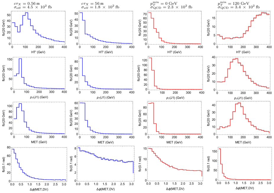
Figure 4: Distributions of events with one DV in iso-region before defining a SR_Y/CR_Y split, with $\sqrt{s}=13\;\mathrm{TeV}$ and $m_{X}=25\;\mathrm{GeV}$. $p_{T}(J_{1})$ refers to the highest jet $p_{T}$ in the event. First column: BSM events with short lifetime (56 cm). Second column: BSM events with long lifetime (56 m). Third column: QCD background events under pessimistic assumption ($p_{T}^{\mathrm{min}}=0\;\mathrm{GeV}$). Fourth column: QCD background events under optimistic assumption ($p_{T}^{\mathrm{min}}=120\;\mathrm{GeV}$). $\sigma_{\mathrm{eff}}$ is the effective signal cross-section of events with at least one detected DV in the Muon System, after geometric, trigger and detection efficiencies are taken into account (setting $\mathrm{Br}(h\to XX)=1$), see Section III.2.1. $\sigma_{\mathrm{QCD}}$ is the cross-section of SM QCD background in the shown kinematic region as estimated using the methods outlined in Section III.2.2.

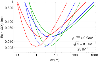
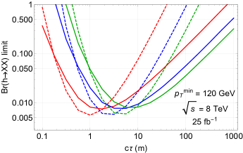
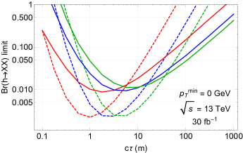
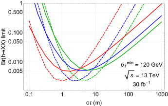
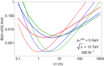
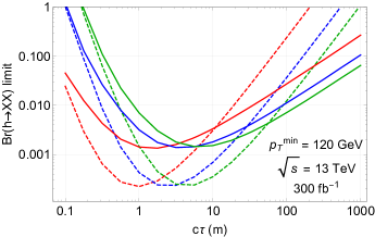
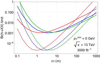
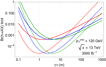
Figure 5: Limit projections for the data-driven search for a single DV in the ATLAS Muon Spectrometer (solid lines) compared to an assumed background-free search for two DVs (dashed lines). For comparison with existing limits ATLAS Collaboration (2015a), the top row shows limits that may have been achieved by performing this search at the LHC run 1. The left (right) column corresponds to the pessimistic (optimistic) choice of QCD background, both normalized to give 3000 background events at the LHC run 1.

For the pessimistic analysis, additional kinematic cuts on the events in SR_Y with $\Delta\phi(\mathrm{MET},\mathrm{DV})>1.5$ (corresponding to region A in Fig. 2) can lead to very slight increases in sensitivity compared to a simple counting experiment in SR_Y with the background prediction derived from the observed events in CR_Y (region C in Fig. 2). We find the two most useful strategies to be (a) no further cuts, and (b) $H_{T}^{\prime}>80\;\mathrm{GeV}$. This may be indicative of the kinds of cuts one might perform in a real experimental analysis, but the details should be taken lightly, given the crude nature of our fake-DV background simulation. The resulting limits on $\mathrm{Br}(h\to XX)$ are shown in the left column of Fig. 5 .

For the optimistic analysis, SR_Y with $\Delta\phi(\mathrm{MET},\mathrm{DV})>1.0$ is so signal-enriched that no cuts are necessary to enhance sensitivity even for high luminosities. The resulting limits on $\mathrm{Br}(h\to XX)$ are shown in the right column of Fig. 5.

These limit projections confirm our expectation that the data-driven search for one DV represents a great improvement at long $X$ proper lifetimes, yielding limits orders of magnitude better than even a background-free search for two DVs in the Muon Spectrometer. The limits in the optimistic QCD case are noticably better than the pessimistic QCD limits, especially for modest proper lifetimes less than about one meter, due to the better intrinsic separation of signal and background. However, the difference in the projected limits from the two very different modelings of the QCD background is only about a factor of $2$, indicating that our strategy is quite robust. The background-free sensitivity projections of the two-DV search scales with luminosity $\mathcal{L}$, while for the one-DV search with data-driven background estimates the limit scales like $\sqrt{\mathcal{L}}$. At high luminosities, the sensitivity gain of the one-DV search relative to the two-DV search is therefore reduced, but even in this case the former has superior reach at long lifetimes. (Our estimates for the two-DV search are also likely to be optimistic in the case of the HL-LHC due to the different running conditions.)

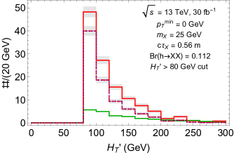
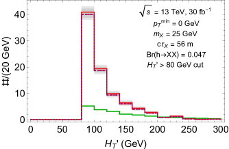
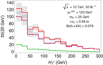
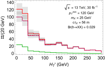
Figure 6: $H_{T}^{\prime}$ distributions, at the 13 TeV LHC with $30{\ \rm fb}^{-1}$ of luminosity, in signal region A. For the pessimistic QCD case with $p_{T}^{\mathrm{min}}=0\;\mathrm{GeV}$ and an additional $H_{T}^{\prime}>80\;\mathrm{GeV}$ cut (top), and for the optimistic QCD case with $p_{T}^{\mathrm{min}}=120\;\mathrm{GeV}$ (bottom). The mass of the LLP is $m_{X}=25\;\mathrm{GeV}$, with a short lifetime of $c\tau=56\mathrm{cm}$ on the left and a long lifetime of $c\tau=56m$ on the right. Green: $h\to XX$ signal, Red: QCD background prediction from CR_Y, including BSM contamination of region C. Dashed red: QCD background prediction if there were no BSM contamination in region C. Purple dotted: truth-level QCD in region A. Gray shading indicates the $2\sigma$ uncertainty in the SM prediction from limited region C statistics, which is significant in the lowest $H_{T}^{\prime}$ bin in the optimistic QCD case.

We close this discussion by commenting on BSM contamination in the control regions. Fig. 6 shows the distribution of BSM $h\to XX$ and SM events in region A, for long and short lifetimes with $m_{X}=25\;\mathrm{GeV}$. In each case, $\mathrm{Br}(h\to XX)$ is chosen to be at the 95% CL limit projection. The solid red histogram shows the QCD prediction derived from the observation in region C, while the dashed red histogram shows what the prediction would be if there were no BSM events in the CR_Y. In the short lifetime case, a significant fraction of the background prediction results from BSM events falling into the control region. This underscores why sensitivity decreases sharply for proper lifetimes less than a meter. As discussed in Section III.1, we expect alternative definitions for the CR_Y to be more useful in this case.

In deriving our limit projections for the single-DV search, we simply took the expected observation in the CR_Y at face-value to predict the SM background. In a full analysis, sensitivity would be further improved by taking into account the CR_Y contamination for each assumption of $\mathrm{Br}(h\to XX)$, as discussed in Sections II.3 and IV.

III.3 Reach Improvement for Theories of Neutral Naturalness

Theories of Neutral Naturalness, so-called because they solve the little hierarchy problem through top partners that are neutral under the SM strong force, are among the best-motivated theories that give rise to Higgs decays to LLPs. These theories predict (sub-)weak-scale degrees of freedom that may carry either electroweak charges, as in Folded SUSY Burdman et al. (2007) and the Quirky Little Higgs Cai et al. (2009), or no SM charges at all, as realized in the Twin Higgs model Chacko et al. (2006). As LHC Run-1 results have reduced significantly the viable natural parameter space for colored top partners, models of Neutral Naturalness, which generalize the usual assumptions about top partner phenomenology, have come into new prominence as viable solutions to the hierarchy problem. Most importantly for our current purposes, Higgs decays to LLPs are among the leading signatures of these models, in many cases offering the best window into the physics of SM-neutral top partners, and thereby onto the stability of electroweak scale. This makes theories of Neutral Naturalness one of the most exciting motivations for LLP searches at the LHC in general, and for the signal $h\to XX$ in particular. In this subsection we demonstrate how the sensitivity gains from the search for a single DV in the MS proposed above translate to expanded reach in the parameter space of the Fraternal Twin Higgs model (FTH) Craig et al. (2015).

The most important low-lying fundamental degrees of freedom in the FTH are SM singlet top and bottom partners $T$ and $B$, which are charged under a mirror QCD gauge group and couple to the Higgs via a mixing-suppressed Yukawa interaction. The Higgs boson acts as a portal between the SM and the mirror QCD sector, through both its direct Yukawa couplings to mirror quarks and the resulting effective coupling to mirror gluons. These couplings enable low-lying mirror hadron states to be produced in exotic Higgs decays. These mirror hadrons decay back to the SM via an off-shell Higgs, and are generically long-lived Craig et al. (2015); Morningstar and Peardon (1999); Juknevich et al. (2009); Juknevich (2010). The phenomenology of exotic Higgs decays in the FTH model depends in detail on the relative values of the mass of the mirror bottom, $m_{B}$, and the strong coupling scale of mirror QCD, $\Lambda_{QCD^{\prime}}$, and can be quite complicated. The low-lying hadrons may be mirror glueballs, mirror bottomonia, or a mixture of both; the total Higgs branching fraction into mirror hadrons can be controlled by either the mirror bottom Yukawa coupling or the (mirror-top-induced) effective coupling to mirror gluons; the lifetime of the mirror glueballs depends on both $\Lambda_{QCD^{\prime}}$ and the mass of the mirror top $m_{T}$; and non-perturbative physics describing hadronization in the mirror sector can introduce large uncertainties. Some of these issues were discussed in Craig et al. (2015); Curtin and Verhaaren (2015), and will be explored in detail in an upcoming study Curtin and Tsai (2016). Here, we merely give an abbreviated preview of those results by focusing on a region of parameter space where the search for a single DV in the MS offers obvious and unique advantages.

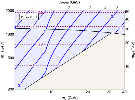
Figure 7: Partial phase space of FTH model with $y_{b}^{\prime}=y_{b}^{\mathrm{SM}}$. Blue background shading: YEGP phase of the FTH model. Brown shading, and other areas with $m_{0}>40\;\mathrm{GeV}$: more complicated exotic Higgs decay scenarios that will be explored in Curtin and Tsai (2016). Blue contours: proper lifetime $\log_{10}(c\tau/\mathrm{meter})$ of $0^{++}$ glueballs. Purple contours: $\log_{10}$ of the perturbatively calculated exotic Higgs branching ratio to mirror gluons via intermediate mirror bottoms. Below the horizontal black line the intermediate state can be multiple mirror bottomonia, while above the black line it can be an excited quirky bound state of two mirror bottoms which annihilates to glueballs.

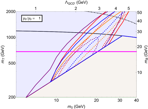
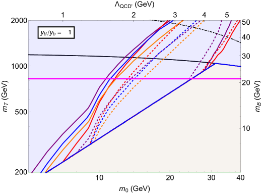
LHC $300{\ \rm fb}^{-1}$ HL-LHC $3000{\ \rm fb}^{-1}$

Figure 8: Colored contours: reach of various proposed searches for LLPs in the YEGP phase of the FTH model (blue background shading, see Fig. 7) at the LHC with $300{\ \rm fb}^{-1}$ (left) and $3000{\ \rm fb}^{-1}$ (right) of luminosity, using results from Curtin and Verhaaren (2015) and the limits for searches in the MS from this paper. Solid (dashed) contours indicate optimistic (pessimistic) assumptions for the number of $0^{++}$ glueballs produced, see text. Magenta line shows reach of Higgs coupling constraints for that luminosity. Projections above the black dot-dashed line should be treated with caution due to possible non-perturbative suppressions of the exotic Higgs decay branching ratio. Similar suppressions could occur for some glueball masses above 40 GeV.

The plots in Figs. 7 and 8 show part of the phase space of exotic Higgs decays in the FTH model for the $\mathbb{Z}_{2}$ symmetric choice of mirror bottom Yukawa $y_{b}^{\prime}=y_{b}^{\mathrm{SM}}$. With this parameter fixed, the top partner mass (left vertical axis) determines both the mirror Higgs vev $f$ and the bottom partner mass (right vertical axis). The confinement scale $\Lambda_{\mathrm{QCD}^{\prime}}$ (top horizontal axis) of mirror QCD is an unknown parameter that depends on both the full mirror sector spectrum and the UV completion, and determines the mass $m_{0}\approx 7\Lambda_{\mathrm{QCD}^{\prime}}$ of the lightest mirror glueball $G_{0}=0^{++}$ (bottom horizontal axis). At each point in this $(m_{0},m_{T})$-plane, all mirror hadron masses, lifetimes, and exotic Higgs branching fractions are determined (with the exception of additional bottomonium decay modes if mirror leptons are light). Fig. 7 shows the exotic Higgs decay branching fraction to mirror glue, and the lifetime of $0^{++}$ glueballs. At glueball masses below the $\bar{b}b$ threshold, the proper lifetimes become extremely long, making this the most challenging regime for LLP searches.

In the brown shaded regions, both glueballs and mirror bottomonia $\eta$ are light enough to be produced in exotic Higgs decays, and can potentially mix with each other. For $m_{0}>40\;\mathrm{GeV}$, there are regions where glueballs are either not produced or decay to mirror bottomonia, meaning that all exotic Higgs decays produce bottomonium final states. These regions, as well as different choices of $y_{b}^{\prime}$, will be explored in Curtin and Tsai (2016).

The blue regions are the area of most interest for single DV searches in the MS. Here, the decay $h\to B\bar{B}$ is perturbatively allowed. The $\bar{B}B$ states either produce mirror bottomonia, which can decay to glueballs, or a so-called quirk bound state Kang and Luty (2009); Burdman et al. (2008); Harnik and Wizansky (2009); Harnik et al. (2011); Burdman et al. (2015); Chacko et al. (2015), which can be thought of as a single very excited bottomonium, that promptly annihilates to glueballs. In either case, the exotic Higgs decay branching fraction is dictated by the mirror bottom Yukawa, and is therefore rather large ($\sim$ 1 - 10$\%$ for $m_{T}\lesssim\;\mathrm{TeV}$), but the final states are the long-lived glueballs, which decay to the SM via the highly suppressed top partner loop and an off-shell Higgs boson, with proper decay lengths ranging from $\sim$ 1000 km to $\sim$ millimeters for glueball masses $\sim 5-60\;\mathrm{GeV}$. The combination of relatively large LLP production rates and long lifetimes makes this phase of the FTH, which we refer to as “Yukawa-enhanced glueball production” (YEGP), an ideal benchmark for our single-DV searches.

Ref. Curtin and Verhaaren (2015) examined the reach of displaced searches at the LHC for glueballs in theories of Neutral Naturalness, assuming the exotic Higgs decays are mediated by the top partner loop. Three searches were found to have great combined coverage of the parameter space:

1. a search for 1 DV in the MS, with an additional DV in either the MS or IT;

2. a search for 1 DV in the IT with minimum distance of 4 cm from the IP (modeled on current displaced vertex reconstruction capability at ATLAS), with VBF jets for triggering;

3. a search for 1 DV in the IT with a minimum distance of 50 $\mu m$ from the IP, with an additional lepton for triggering.

The first search has already been performed by ATLAS at LHC Run-1 ATLAS Collaboration (2015a), while the other two are proposals for future searches that could be performed by either general-purpose LHC experiment. In particular, the third search demonstrates how much sensitivity could be gained if very short displacements could be reconstructed. The search projections are pessimistic in the sense that ATLAS Run-1 reconstruction efficiencies are assumed for DVs in the IT for the entire LHC program, and optimistic in the sense of assuming no backgrounds.

We apply the same methodology as Curtin and Verhaaren (2015) to the YEGP phase of the FTH. This involves making the pessimistic assumption that only two glueballs are produced per exotic Higgs decay (for small $m_{0}$, showering will likely produce more). The projected exclusions of the background-free (DV in IT + VBF) and (DV in IT + lepton) searches in the YEGP phase are shown in Fig. 8 as blue and orange contours. The corresponding exclusions from a background-free search for 2 DVs in the MS and our proposed search for 1 DV in the MS (see Fig. 5) are shown as red and purple contours, respectively. Solid contours indicate reach if all glueballs are the lightest $0^{++}$ state, while dashed lines make the more pessimistic assumption that $\sim 10\%$ of glueballs are $0^{++}$ when all states are kinematically available . Finally, limits above the dot-dashed black should be treated with caution due to non-perturbative suppressions of the exotic Higgs branching fraction compared to the perturbative rate we assume, which will be discussed in more detail in Curtin and Tsai (2016). Similar suppressions could occur for some glueball masses above 40 GeV, see Curtin and Verhaaren (2015). Finally, we also indicate the exclusion reach of Higgs coupling measurements on the FTH model, derived using the profile likelihood method Cowan et al. (2011) and sensitivity projections for 300 and 3000 ${\ \rm fb}^{-1}$ from Vidal (2014); Flechl (2015) .

Fig. 8 makes clear that our proposed inclusive search for 1 DV in the MS significantly extends the LHC reach in the FTH parameter space to glueball masses as low as 6 GeV, and increases the top partner mass reach by several hundred GeV compared to other searches. These significant gains into the most challenging parts of FTH parameter space, where glueballs have very long lifetime and mostly escape the detector, strongly motivate implementation of this search. At the HL-LHC, sensitivity improvements compared to the background-free (DV in IT + VBF) search seem more modest. However, the background-free assumption for the latter search is likely overly optimistic, especially at high instantaneous luminosities, while our projections for the 1DV search already take different running conditions into account in estimating backgrounds. Therefore, it is very likely that the 1DV search will perform significantly better at low glueball masses than the 1DV + lepton or jets searches.

IV Directions for a Future Search Program

In Section II, we explained how a data-driven ABCD method can be used to obtain differential background estimates for LLP searches in the MS. We demonstrated the technical details of such an analysis and the resulting potential gains in sensitivity, using a particularly well-motivated (and challenging) signal model of LLP pair production from the decay of a Higgs-like scalar in Section III. We now generalize this method to outline a possible comprehensive search program for LLPs.

There are a large number of theories that yield LLPs with detector-scale lifetimes. We begin by surveying several of the best motivated classes of such theories, and then discuss how they can be mapped onto a simpler signature space for displaced decays. This signature space then naturally suggests a set of signal-like and control-like regions defined by observables $Y_{i}$, which can be used to implement flexible and model-independent searches for displaced decays in the MS. We conclude this section by commenting on how this approach could be extended to searches for displaced decays in other detector systems.

IV.1 Theories yielding long-lived signatures

A wide variety of well-motivated theories of BSM physics predict LLPs. Perhaps the most familiar framework yielding LLPs is the MSSM, which can easily yield displaced superpartner decays through a variety of mechanisms:

• In split SUSY, the decay rate of (sub-)TeV gaugino and higgsino superpartners is suppressed by heavy sfermions with masses in excess of 1000 TeV, leading to displaced decays Arvanitaki et al. (2013); Arkani-Hamed et al. (2012); Rolbiecki and Sakurai (2015).

• In models of gauge-mediated SUSY-breaking (GMSB), NLSP decays can become displaced when the scale of supersymmetry breaking is sufficiently high Giudice and Rattazzi (1999).

• Models with $R$-parity violation (RPV) Barbier et al. (2005) often feature very small couplings that in some cases can be generated dynamically Csaki et al. (2014), leading to detector-scale LSP lifetimes. Such small baryon-number-violating RPV couplings are independently well-motivated by models of baryogenesis Bouquet and Salati (1987); Campbell et al. (1991); Cui and Sundrum (2013); Barry et al. (2014); Ipek and March-Russell (2016).

• In anomaly-mediated SUSY-breaking (AMSB) Chen et al. (1997); Giudice et al. (1998); Randall and Sundrum (1999), the neutral wino LSP is nearly degenerate with the charged wino, resulting in a macroscopic lifetime for the charged state.

With this panoply of well-motivated mechanisms to produce displaced decays, the MSSM is a very effective generator of displaced signatures: most prompt SUSY signatures can be readily translated into well-motivated displaced signatures through one of these mechanisms simply by giving the last stage of the cascade decay a macroscopic lifetime.

Another large class of models that generically features long-lived particles are weak-scale hidden sectors (Hidden Valleys) Strassler and Zurek (2007, 2008); Strassler (2006); Han et al. (2008); Strassler (2008a, b), which include the theories of Neutral Naturalness discussed in the last section. Possible portals into hidden sectors are provided by the $h$ and $Z$ bosons coupling or mixing with the hidden states, as well as through BSM states that have tree-level couplings to both sectors. Such BSM mediator particles can be either singly produced (e.g., a $Z^{\prime}$), or pair-produced (e.g., new vector-like fermions), corresponding to resonant and non-resonant LLP pair production. These models frequently contain strong dynamics in the hidden sector, which can lead to variable and potentially high LLP multiplicities through hidden sector showers. It is also common in these models for hidden sector states to exhibit a hierarchy of proper lifetimes.

Combining these two classes of ideas to extend the MSSM with a (softly-broken supersymmetric) weak-scale hidden sector is well-motivated by dark matter model-building Baumgart et al. (2009); Chan et al. (2012) and as a way to reconcile natural SUSY with constraints from LHC Run-1 (Stealth SUSY) Fan et al. (2011). These theories can lead to even more varied LLP phenomenology. Typically in these theories, it is the LSP (or, more exactly, the Lightest Ordinary Superpartner “LOSP”) that mediates decays into the hidden sector Strassler (2006). Here displacement can arise in the decay of the LOSP into the hidden sector as well as in the decay of one or more of the hidden sector states back to the SM, and the detector signature of the displaced decay is largely controlled by the detailed content of the hidden sector.

Cosmology provides additional motivation for displaced decays at colliders. As already mentioned, baryogenesis can motivate long-lived particles that decay via tiny baryon-number-violating interactions Cui and Sundrum (2013); Barry et al. (2014); Cui and Shuve (2015); Ipek and March-Russell (2016). A detector-scale lifetime can also be directly related to the DM relic abundance in some models of freeze-in DM Co et al. (2015), or as a consequence of a small mass splitting between two dark states to enable efficient coannihilation in the early universe Falkowski et al. (2014). Models with heavy ($m\gtrsim 10$ GeV) sterile neutrinos generically predict macroscopic decay lengths for the heavy right-handed neutrinos. Depending on the details of the model, sterile neutrinos can be dominantly singly-produced through charged-current interactions Helo et al. (2014); Antusch et al. (2016) or pair-produced through a mediator such as the SM Higgs or a BSM vector boson Graesser (2007a, b); Maiezza et al. (2015); Batell et al. (2016).

IV.2 A signature space for displaced searches

From the point of view of designing a flexible search program, what matters is not the theoretical motivation for the displaced decay but the detector signature. To a very large degree, this is controlled by two features of any given model of new physics: (i) production, and (ii) decay. As the variety of theories listed above suggests, the lifetime of any given LLP can effectively be regarded as a free parameter. Focusing on displaced decays in the MS as the case of interest, we further note that here searches are insensitive to the fine details of the LLP decay. Thus for searches in the MS, the detector signatures will largely be controlled by the production mechanism, which determines overall expectations for signal rates well as the number and type of AOs. These AOs in turn will control the useful choice(s) of $Y$, the variable that along with the distinction between iso- and non-iso-events defines the signal and control regions in Fig. 2.

Common production modes for LLPs $X$ include:

• The pair-production of a parent particle $P$ that then decays to $X$ + SM particles. This production mode includes the vast majority of SUSY models, as well as models that pair-produce BSM mediator states, including some Hidden Valley theories and the cosmologically motivated models of Refs. Co et al. (2015); Falkowski et al. (2014). If $P$ is colored, or if it is produced in the decays of colored particles, then the typical AOs are jets; if $P$ can only be produced through its electroweak interactions with the SM, then the most useful AOs are likely to be leptons or photons.

• The production of a single parent particle $P$ that decays via $P\to XX$. This production mode can dominate in many Hidden Valley theories, including theories of Neutral Naturalness. If $P$ is a Higgs-like state (either the SM-like Higgs, or a state that mixes with it) as in Section III, there are no distinctive AOs. If $P$ is a vector $Z^{\prime}$ that mixes with SM gauge bosons via either mass or kinetic mixing, Drell-Yan (DY)-like production dominates, again without distinctive AOs (see e.g., Curtin et al. (2015); Clarke (2015); Argüelles et al. (2016); ATLAS Collaboration (2014a)). However, in fermiophobic $Z^{\prime}$ scenarios production could require an associated SM $W,Z$ or $\gamma$.

• LLPs can also be singly produced, generally in combination with some AOs in the event. For example, if BSM states $(X_{1},X_{2})$ form an $SU(2)_{L}$ doublet where $X_{1}$ is the neutral LLP, they can be produced in a DY-like process $W^{*}\to X_{1}X_{2}\to X_{1}X_{1}+$ soft, as in AMSB. Another way to singly produce an LLP $X$ at a non-negligible rate is the decay of a parent $P$ into a hidden sector, such as $h\to X_{1}X_{2}$, with $X_{1}$ long-lived and $X_{2}$ promptly decaying to the SM. Since it is generic for different states in a confining hidden sector to have order(s) of magnitude differences in their lifetimes, this possibility should not be overlooked. Single production is also common in models of weak-scale sterile neutrinos, where the dominant production mechanism can be $pp\to N\ell$.

This, together with our findings from Section III for LLPs produced in the decay of a Higgs-like scalar, suggest the following simple dictionary of choices for the variable $Y$:

• The number of leptons $N_{\ell}$. The simplest SR_Y is defined by requiring $N_{\ell}>0$.

• The number of light or heavy flavor jets $N_{j},N_{b}$. It may also be useful to include kinematic properties such as VBF tagging or $p_{T}$ cuts. The simplest SR_Y is defined by requiring $N_{j}$ or $N_{b}>0$.

• The number of tagged/reconstructed SM $W$, $Z$, $\gamma$ bosons, with the simplest SR_Y requiring at least one of these.

• To target signal models that dominantly do not produce AOs, the kinematic variable $\Delta\phi(\mathrm{MET},\mathrm{DV})$ and the veto on unusual objects in the calorimeters or tracker, as discussed in Section III.1.

Our toy analysis in Section III estimated the sensitivity of an analysis using $Y=\Delta\phi(\mathrm{MET},\mathrm{DV})$. In more straightforward cases, simple scaling arguments can give an idea of the achievable sensitivity. Consider the case of $Y$ = number of leptons or $W,Z$. The inclusive QCD cross section for events with one DV in the MS is $\sim O(100\,\mathrm{fb})$ at 13 TeV, see Fig. 4. The inclusive production cross section for $W,Z$ bosons, which are also the dominant source of leptons, is about $10^{-5}$ times smaller than inclusive QCD jet production ATLAS Collaboration (2012c). We can therefore expect a signal region defined by requiring a lepton, $W$, or $Z$ to have fewer background events than the $h\to XX$ analysis by a similar factor. With such a $\sim 10^{-3}\ \mathrm{fb}$ background cross section, searches for a DV in the MS + lepton or $Z,W$ are likely to be nearly background-free even with more than 300 ${\ \rm fb}^{-1}$ of luminosity. On the other hand, a search for LLPs produced in association with at least one $b$-jet defines a signal region with $Y=N_{b}\geq 1$. In this case, the background reduction is a more modest factor of $\sim 30$ CMS Collaboration (2012b). This will give sensitivity to the pair-production of colored parent particles $P$ with masses in excess of 1 TeV with only 30 ${\ \rm fb}^{-1}$ of LHC13 luminosity. The sensitivity for LLPs dominantly produced in association with light jets is more challenging to estimate, and will depend on the spectrum. In the presence of large mass splittings in the decay chain that produces the LLPs, variables sensitive to the acoplanarity of the jets + DV system are attractive candidates for defining a robust signal-like/control-like region split. On the other hand, in compressed regions of parameter space where associated jets are soft, $\Delta\phi(\mathrm{MET},\mathrm{DV})$ can be the most useful choice of $Y$.

To realize maximum sensitivity, a detailed analysis along the lines of that sketched in Section III would be implemented for each signal model under consideration. However, it is worth emphasizing that for each of the above choices of $Y$, with associated definitions of the regions A,B,C,D in Fig. 2, BSM contributions to regions A and C can be made visible simply by examining the ratio

$$\mathcal{R}_{Y}(H_{T}^{\prime},\ldots)=\frac{r_{\mathrm{non\mathchar 45\relax iso\to iso}}^{\mathrm{CR}_{Y}}(H_{T}^{\prime},\ldots)}{r_{\mathrm{non\mathchar 45\relax iso\to iso}}^{\mathrm{SR}_{Y}}(H_{T}^{\prime},\ldots)}$$ (27)

of rescaling functions as computed in SR_Y and CR_Y without accounting for any BSM contributions. The $\ldots$ indicates that this ratio could be observed as a function of other variables as well, if statistics are sufficient. An excess in A but not in C (or vice versa) would show up as a positive (negative) deviation in the $\mathcal{R}_{Y}$ distribution from unity. This is a flexible and fully model-independent way of searching for deviations from SM expectations, with the potential to direct future targeted analyses if interesting deviations are observed.

IV.3 Generalization to other Detector Systems

The discussion in this paper centers on the detection of LLPs decaying in the MS, due to the availability of both signal and orthogonal triggers at ATLAS, and the unique advantage conferred by such searches in probing LLPs with very long lifetimes. However, the general strategy we outline in Section II, and a model-independent set of searches as suggested in Section IV.2, could be adapted to LLP searches using other detector subsystems as well.

For LLPs decaying in the calorimeters, the isolation criteria used to distinguish between iso- and non-iso-events operate similarly to the criteria for the MS by quantifying the amount of activity upstream of the DV-candidate. A signal trigger already exists at ATLAS ATLAS Collaboration (2013c), and an orthogonal trigger for non-iso-events could in principle be implemented as well.

In general, this search strategy can also be implemented in any detector subsystem where the triggering strategy does not rely on the LLP decay directly, which would be the case, e.g., when using the single lepton trigger to search for displaced decays in the tracker (as suggested for exotic Higgs decays Curtin and Verhaaren (2015); Csaki et al. (2015b)). In that case, different offline reconstruction criteria could separate iso from non-iso-events, in the cases where the background rate is large enough to necessitate implementation of the data-driven background estimation strategy presented here. This would likely be relevant, for example, when reconstructing macroscopic decay lengths less than a mm. Such an analysis would be very challenging, but is highly motivated in many models, see, e.g., Curtin and Verhaaren (2015).

V Conclusions

Searches for long-lived particles (LLPs) are motivated in a large variety of BSM scenarios connected to naturalness, dark matter, baryogenesis, and other fundamental mysteries of particle physics. In this paper we suggest use of existing ATLAS triggers to conduct a search for a single LLP decaying in the MS, which offers great improvements in sensitivity over existing searches for long proper lifetimes. Such a search has to contend with sizable SM background from QCD jets faking DVs in the MS, and we propose a data-driven approach to obtain predictions for those backgrounds that can be made differential in important kinematic variables.

We explicitly implement our strategy for the specific case where two LLPs are pair-produced in the exotic decay of the 125 GeV Higgs boson (or a general Higgs-like scalar). This is a very well-motivated scenario that arises, e.g., in theories of Neutral Naturalness or general Hidden Valleys. It also represents the most challenging application of our strategy, since the inclusive production mode prohibits a straightforward definition of signal and control regions by, for example, selecting for accompanying prompt leptons or jets. Even so, our study demonstrates large sensitivity gains at long lifetimes compared to a background-free search for two DVs in the MS. This leads to significantly expanded reach in the parameter space of BSM models, as we have explicitly demonstrated in the case of Neutral Naturalness for the Fraternal Twin Higgs model.

Our strategy lends itself to the formulation of a model-independent search program for LLPs decaying in the MS, in analogy to the simplified model framework for prompt searches. In our approach, different signal model classes are categorized by the production mode of the LLP(s), and deviations from the SM expectation are parameterized as deviations of a data-driven ratio $\mathcal{R}_{Y}$ from unity, see Eq. (27). Furthermore, our approach can be generalized to LLP searches in other detector systems such as the calorimeters and the tracker. This has the potential to significantly expand both the breadth and the sensitivity of the search program for long-lived particles at the LHC.

Acknowledgements

D.C. would like to thank Sarah Eno for useful conversation. A.C. acknowledges the support of the Swiss National Science Foundation under the grant 200020_156083. D.C. is supported by National Science Foundation grant No. PHY-1315155 and the Maryland Center for Fundamental Physics. H.L. and H.R. acknowledge the support of National Science Foundation grant PHY-1509257. The work of J.S. is supported in part by DOE grant DE-SC0015655.

References

- Arvanitaki et al. (2013) A. Arvanitaki, N. Craig, S. Dimopoulos, and G. Villadoro, JHEP 02, 126 (2013), arXiv:1210.0555 [hep-ph] .
- Arkani-Hamed et al. (2012) N. Arkani-Hamed, A. Gupta, D. E. Kaplan, N. Weiner, and T. Zorawski, (2012), arXiv:1212.6971 [hep-ph] .
- Giudice and Rattazzi (1999) G. F. Giudice and R. Rattazzi, Phys. Rept. 322, 419 (1999), arXiv:hep-ph/9801271 [hep-ph] .
- Barbier et al. (2005) R. Barbier et al., Phys. Rept. 420, 1 (2005), arXiv:hep-ph/0406039 [hep-ph] .
- Csaki et al. (2014) C. Csaki, E. Kuflik, and T. Volansky, Phys. Rev. Lett. 112, 131801 (2014), arXiv:1309.5957 [hep-ph] .
- Fan et al. (2011) J. Fan, M. Reece, and J. T. Ruderman, JHEP 1111, 012 (2011), arXiv:1105.5135 [hep-ph] .
- Bouquet and Salati (1987) A. Bouquet and P. Salati, Nucl. Phys. B284, 557 (1987).
- Campbell et al. (1991) B. A. Campbell, S. Davidson, J. R. Ellis, and K. A. Olive, Phys. Lett. B256, 484 (1991).
- Cui and Sundrum (2013) Y. Cui and R. Sundrum, Phys. Rev. D87, 116013 (2013), arXiv:1212.2973 [hep-ph] .
- Barry et al. (2014) K. Barry, P. W. Graham, and S. Rajendran, Phys. Rev. D89, 054003 (2014), arXiv:1310.3853 [hep-ph] .
- Ipek and March-Russell (2016) S. Ipek and J. March-Russell, (2016), arXiv:1604.00009 [hep-ph] .
- Strassler and Zurek (2007) M. J. Strassler and K. M. Zurek, Phys.Lett. B651, 374 (2007), arXiv:hep-ph/0604261 [hep-ph] .
- Strassler and Zurek (2008) M. J. Strassler and K. M. Zurek, Phys.Lett. B661, 263 (2008), arXiv:hep-ph/0605193 [hep-ph] .
- Strassler (2006) M. J. Strassler, (2006), arXiv:hep-ph/0607160 [hep-ph] .
- Han et al. (2008) T. Han, Z. Si, K. M. Zurek, and M. J. Strassler, JHEP 0807, 008 (2008), arXiv:0712.2041 [hep-ph] .
- Strassler (2008a) M. J. Strassler, (2008a), arXiv:0801.0629 [hep-ph] .
- Strassler (2008b) M. J. Strassler, (2008b), arXiv:0806.2385 [hep-ph] .
- Curtin et al. (2015) D. Curtin, R. Essig, S. Gori, and J. Shelton, JHEP 1502, 157 (2015), arXiv:1412.0018 [hep-ph] .
- Clarke (2015) J. D. Clarke, JHEP 10, 061 (2015), arXiv:1505.00063 [hep-ph] .
- Argüelles et al. (2016) C. A. Argüelles, X.-G. He, G. Ovanesyan, T. Peng, and M. J. Ramsey-Musolf, (2016), arXiv:1604.00044 [hep-ph] .
- Burdman et al. (2007) G. Burdman, Z. Chacko, H.-S. Goh, and R. Harnik, JHEP 0702, 009 (2007), arXiv:hep-ph/0609152 [hep-ph] .
- Cai et al. (2009) H. Cai, H.-C. Cheng, and J. Terning, JHEP 0905, 045 (2009), arXiv:0812.0843 [hep-ph] .
- Chacko et al. (2006) Z. Chacko, H.-S. Goh, and R. Harnik, Phys.Rev.Lett. 96, 231802 (2006), arXiv:hep-ph/0506256 [hep-ph] .
- Cui and Shuve (2015) Y. Cui and B. Shuve, JHEP 02, 049 (2015), arXiv:1409.6729 [hep-ph] .
- Craig et al. (2015) N. Craig, A. Katz, M. Strassler, and R. Sundrum, (2015), arXiv:1501.05310 [hep-ph] .
- Liu and Tweedie (2015) Z. Liu and B. Tweedie, JHEP 06, 042 (2015), arXiv:1503.05923 [hep-ph] .
- Csaki et al. (2015a) C. Csaki, E. Kuflik, S. Lombardo, O. Slone, and T. Volansky, JHEP 08, 016 (2015a), arXiv:1505.00784 [hep-ph] .
- Curtin and Verhaaren (2015) D. Curtin and C. B. Verhaaren, (2015), arXiv:1506.06141 [hep-ph] .
- Evans and Shelton (2016) J. A. Evans and J. Shelton, JHEP 04, 056 (2016), arXiv:1601.01326 [hep-ph] .
- ATLAS Collaboration (2012a) ATLAS Collaboration, Phys. Rev. Lett. 108, 251801 (2012a), arXiv:1203.1303 [hep-ex] .
- ATLAS Collaboration (2013a) ATLAS Collaboration, Phys. Lett. B721, 32 (2013a), arXiv:1210.0435 [hep-ex] .
- ATLAS Collaboration (2013b) ATLAS Collaboration, Phys. Lett. B719, 280 (2013b), arXiv:1210.7451 [hep-ex] .
- ATLAS Collaboration (2015a) ATLAS Collaboration, Phys. Rev. D92, 15 (2015a), arXiv:1504.03634v2 .
- ATLAS Collaboration (2015b) ATLAS Collaboration, Phys.Lett. B743, 15 (2015b), arXiv:1501.04020 [hep-ex] .
- ATLAS Collaboration (2014a) ATLAS Collaboration, JHEP 11, 088 (2014a), arXiv:1409.0746 [hep-ex] .
- ATLAS Collaboration (2015c) ATLAS Collaboration, Phys. Rev. D92, 072004 (2015c), arXiv:1504.05162 [hep-ex] .
- CMS Collaboration (2012a) CMS Collaboration, Phys. Lett. B713, 408 (2012a), arXiv:1205.0272 [hep-ex] .
- CMS Collaboration (2013) CMS Collaboration, JHEP 02, 085 (2013), arXiv:1211.2472 [hep-ex] .
- CMS Collaboration (2015a) CMS Collaboration, Phys.Rev. D91, 012007 (2015a), arXiv:1411.6530 [hep-ex] .
- CMS Collaboration (2015b) CMS Collaboration, Phys. Rev. D91, 052012 (2015b), arXiv:1411.6977 [hep-ex] .
- Aaij et al. (2015) R. Aaij et al. (LHCb Collaboration), Eur. Phys. J. C75, 152 (2015), arXiv:1412.3021 [hep-ex] .
- CMS Collaboration (2015c) CMS Collaboration, Phys. Rev. Lett. 114, 061801 (2015c), arXiv:1409.4789 [hep-ex] .
- ATLAS Collaboration (2013c) ATLAS Collaboration, JINST 8, P07015 (2013c), arXiv:1305.2284 .
- ATLAS Collaboration (2014b) ATLAS Collaboration, JINST 9, P02001 (2014b), arXiv:1311.7070 .
- Note (1) In case of bandwidth limitations, the non-iso trigger rate can be adjusted to populate the control regions with the necessary statistics.
- Note (2) For example, it may be that is the more useful variable, since it more directly isolates the properties of the individual jet producing the DV, but this detail does not affect our discussion.
- Note (3) If a bin is so small that its expected occupation is much less than 1, then the experimentally derived upper limit on its expected occupation will significantly overestimate . The minimum useful bin width thus depends on the background rate in a given search.
- Aad et al. (2016) G. Aad et al. (ATLAS), JHEP 02, 062 (2016), arXiv:1511.05542 [hep-ex] .
- Curtin et al. (2014) D. Curtin, R. Essig, S. Gori, P. Jaiswal, A. Katz, et al., Phys.Rev. D90, 075004 (2014), arXiv:1312.4992 [hep-ph] .
- ATLAS Collaboration (2015d) ATLAS Collaboration, Expected performance of missing transverse momentum reconstruction for the ATLAS detector at , Tech. Rep. ATL-PHYS-PUB-2015-023 (CERN, Geneva, 2015).
- Andersen et al. (2013) J. R. Andersen et al. (LHC Higgs Cross Section Working Group), (2013), 10.5170/CERN-2013-004, arXiv:1307.1347 [hep-ph] .
- Alwall et al. (2014) J. Alwall, R. Frederix, S. Frixione, V. Hirschi, F. Maltoni, O. Mattelaer, H. S. Shao, T. Stelzer, P. Torrielli, and M. Zaro, JHEP 07, 079 (2014), arXiv:1405.0301 [hep-ph] .
- Sjostrand et al. (2008) T. Sjostrand, S. Mrenna, and P. Z. Skands, Comput.Phys.Commun. 178, 852 (2008), arXiv:0710.3820 [hep-ph] .
- Note (4) In Curtin et al. (2015), it was shown that the matched production of with one extra jet within the EFT framework of the Madgraph model gives a surprisingly accurate representation of the Higgs spectrum.
- ATLAS Collaboration (2012b) ATLAS Collaboration, ATLAS run 1 Luminosity Public Results, Tech. Rep. (CERN, Geneva, 2012).
- ATLAS Collaboration (2015e) ATLAS Collaboration, An imaging algorithm for vertex reconstruction for ATLAS Run-2, Tech. Rep. ATL-PHYS-PUB-2015-008 (CERN, Geneva, 2015).
- ATLAS Collaboration (2015f) ATLAS Collaboration, ATLAS run 2 Luminosity Public Results, Tech. Rep. (CERN, Geneva, 2015).
- ATLAS Collaboration (2014c) ATLAS Collaboration, Primary Vertex and b-Tagging Performance under HL-LHC conditions, Tech. Rep. ATL-PLOT-UPGRADE-2014-003 (CERN, Geneva, 2014).
- Note (5) Systematic uncertainties from weak correlations will be subdominant, as discussed in Section II.3.
- Note (6) The actual experimental sensitivity in the short lifetime regime will also depend on any differences between the contributions to the MET from QCD jets versus particles that decay before the MS, as well as a more detailed treatment of the DV reconstruction efficiency for particles decaying in the outer regions of the HCAL.
- Morningstar and Peardon (1999) C. J. Morningstar and M. J. Peardon, Phys.Rev. D60, 034509 (1999), arXiv:hep-lat/9901004 [hep-lat] .
- Juknevich et al. (2009) J. E. Juknevich, D. Melnikov, and M. J. Strassler, JHEP 0907, 055 (2009), arXiv:0903.0883 [hep-ph] .
- Juknevich (2010) J. E. Juknevich, JHEP 1008, 121 (2010), arXiv:0911.5616 [hep-ph] .
- Curtin and Tsai (2016) D. Curtin and Y. Tsai, (2016), arXiv:TO APPEAR [hep-ph] .
- Kang and Luty (2009) J. Kang and M. A. Luty, JHEP 0911, 065 (2009), arXiv:0805.4642 [hep-ph] .
- Burdman et al. (2008) G. Burdman, Z. Chacko, H.-S. Goh, R. Harnik, and C. A. Krenke, Phys.Rev. D78, 075028 (2008), arXiv:0805.4667 [hep-ph] .
- Harnik and Wizansky (2009) R. Harnik and T. Wizansky, Phys.Rev. D80, 075015 (2009), arXiv:0810.3948 [hep-ph] .
- Harnik et al. (2011) R. Harnik, G. D. Kribs, and A. Martin, Phys.Rev. D84, 035029 (2011), arXiv:1106.2569 [hep-ph] .
- Burdman et al. (2015) G. Burdman, Z. Chacko, R. Harnik, L. de Lima, and C. B. Verhaaren, Phys.Rev. D91, 055007 (2015), arXiv:1411.3310 [hep-ph] .
- Chacko et al. (2015) Z. Chacko, D. Curtin, and C. B. Verhaaren, (2015), arXiv:1512.05782 [hep-ph] .
- Note (7) Thermodynamic arguments Juknevich indicate that of produced glueballs end up in the state, but those predictions are highly uncertain due to our ignorance of pure-gauge hadronization. More sophisticated methods of parameterizing this ignorance have been proposed in Chacko et al. (2015) but they are not suitable for exotic Higgs decays where glueball masses cannot be neglected.
- Cowan et al. (2011) G. Cowan, K. Cranmer, E. Gross, and O. Vitells, Eur. Phys. J. C71, 1554 (2011), [Erratum: Eur. Phys. J.C73,2501(2013)], arXiv:1007.1727 [physics.data-an] .
- Vidal (2014) M. Vidal (CMS Collaboration), in Proceedings, 2nd Conference on Large Hadron Collider Physics Conference (LHCP 2014) (2014) arXiv:1409.1711 [hep-ex] .
- Flechl (2015) M. Flechl (ATLAS Collaboration, CMS Collaboration), Proceedings, 4th Symposium on Prospects in the Physics of Discrete Symmetries (DISCRETE 2014), J. Phys. Conf. Ser. 631, 012028 (2015), arXiv:1503.00632 [hep-ex] .
- Note (8) We use the most optimistic projections for the precision of Higgs coupling measurements (CMS) and assume they apply for both ATLAS and CMS, in order to demonstrate the large gain in sensitivity achieved by the direct searches for displaced vertices.
- Rolbiecki and Sakurai (2015) K. Rolbiecki and K. Sakurai, JHEP 11, 091 (2015), arXiv:1506.08799 [hep-ph] .
- Chen et al. (1997) C. H. Chen, M. Drees, and J. F. Gunion, Phys. Rev. D55, 330 (1997), [Erratum: Phys. Rev.D60,039901(1999)], arXiv:hep-ph/9607421 [hep-ph] .
- Giudice et al. (1998) G. F. Giudice, M. A. Luty, H. Murayama, and R. Rattazzi, JHEP 12, 027 (1998), arXiv:hep-ph/9810442 [hep-ph] .
- Randall and Sundrum (1999) L. Randall and R. Sundrum, Nucl. Phys. B557, 79 (1999), arXiv:hep-th/9810155 [hep-th] .
- Baumgart et al. (2009) M. Baumgart, C. Cheung, J. T. Ruderman, L.-T. Wang, and I. Yavin, JHEP 04, 014 (2009), arXiv:0901.0283 [hep-ph] .
- Chan et al. (2012) Y. F. Chan, M. Low, D. E. Morrissey, and A. P. Spray, JHEP 05, 155 (2012), arXiv:1112.2705 [hep-ph] .
- Co et al. (2015) R. T. Co, F. D’Eramo, L. J. Hall, and D. Pappadopulo, JCAP 1512, 024 (2015), arXiv:1506.07532 [hep-ph] .
- Falkowski et al. (2014) A. Falkowski, Y. Hochberg, and J. T. Ruderman, JHEP 11, 140 (2014), arXiv:1409.2872 [hep-ph] .
- Helo et al. (2014) J. C. Helo, M. Hirsch, and S. Kovalenko, Phys. Rev. D89, 073005 (2014), [Erratum: Phys. Rev.D93,no.9,099902(2016)], arXiv:1312.2900 [hep-ph] .
- Antusch et al. (2016) S. Antusch, E. Cazzato, and O. Fischer, (2016), arXiv:1604.02420 [hep-ph] .
- Graesser (2007a) M. L. Graesser, Phys. Rev. D76, 075006 (2007a), arXiv:0704.0438 [hep-ph] .
- Graesser (2007b) M. L. Graesser, (2007b), arXiv:0705.2190 [hep-ph] .
- Maiezza et al. (2015) A. Maiezza, M. Nemevšek, and F. Nesti, Phys. Rev. Lett. 115, 081802 (2015), arXiv:1503.06834 [hep-ph] .
- Batell et al. (2016) B. Batell, M. Pospelov, and B. Shuve, (2016), arXiv:1604.06099 [hep-ph] .
- ATLAS Collaboration (2012c) ATLAS Collaboration, Phys. Lett. B707, 438 (2012c), arXiv:1109.0525 [hep-ex] .
- CMS Collaboration (2012b) CMS Collaboration, JHEP 04, 084 (2012b), arXiv:1202.4617 [hep-ex] .
- Csaki et al. (2015b) C. Csaki, E. Kuflik, S. Lombardo, and O. Slone, Phys. Rev. D92, 073008 (2015b), arXiv:1508.01522 [hep-ph] .
- (93) J. Juknevich, Phenomenology of pure-gauge hidden valleys at Hadron colliders, Ph.D. thesis, Rutgers U., Piscataway.