Dual approach to circuit quantization using loop charges

Abstract

The conventional approach to circuit quantization is based on node fluxes and traces the motion of node charges on the islands of the circuit. However, for some devices, the relevant physics can be best described by the motion of polarization charges over the branches of the circuit that are in general related to the node charges in a highly nonlocal way. Here, we present a method, dual to the conventional approach, for quantizing planar circuits in terms of loop charges. In this way, the polarization charges are directly obtained as the differences of the two loop charges on the neighboring loops. The loop charges trace the motion of fluxes through the circuit loops. We show that loop charges yield a simple description of the flux transport across phase-slip junctions. We outline a concrete construction of circuits based on phase-slip junctions that are electromagnetically dual to arbitrary planar Josephson junction circuits. We argue that loop charges also yield a simple description of the flux transport in conventional Josephson junctions shunted by large impedances. We show that a mixed circuit description in terms of node fluxes and loop charges yields an insight into the flux decompactification of a Josephson junction shunted by an inductor. As an application, we show that the fluxonium qubit is well approximated as a phase-slip junction for the experimentally relevant parameters. Moreover, we argue that the $0$-$\pi$ qubit is effectively the dual of a Majorana Josephson junction.

I Introduction

Superconducting circuits offer the opportunity to study quantum mechanics on mesoscopic scales unimpeded by dissipation. The great flexibility in design of the superconducting circuits has created the field of circuit quantum electrodynamics where superconducting circuits are used as artificial atoms featuring strongly enhanced light-matter coupling compared to standard cavity QED. Due to weak dissipation, such systems can be described quantum-mechanically with an appropriate Hamiltonian. Finding such a Hamiltonian is the task of circuit quantization. In recent years, there has been a large interest in realizing purely reactive impedances, called “superinductances” $L$, with small parasitic capacitance $C$ such that the characteristic impedance $Z=\sqrt{L/C}$ is much larger than the superconducting resistance quantum $R_{Q}=h/4e^{2}$ masluk:12 . The large impedance leads to a strong localization of charges with fluctuations below the single Cooper-pair limit. This fact makes these large inductances highly relevant for qubits such as the $0$-$\pi$ qubit kitaev:06a or the fluxonium manucharyan:09 with strongly reduced sensitivity to external charge fluctuations. The suppression of charge fluctuations below the single Cooper-pair limit is also relevant for phase slip junctions. Considering the transport of quantized fluxoids as duals of the quantized electron charge tinkham , phase-slip junctions can be understood as electric duals of conventional Josephson junctions with a nonlinear, $2e$-periodic voltage-charge relation $V(Q)$ mooij:06 . Recently, there has been much progress both in the theoretical understanding arutyunov:08 and the experimental realization astafiev:12 ; peltonen:13 ; belkin:11 ; belkin:15 of phase slip junctions using superconducting nanowires. Large characteristic impedances also imply strongly enhanced electric fields in waveguides, allowing an enhanced coupling to qubits like the transmon or efficient nano-mechanical coupling to nanostructures fink:16 ; samkharadze:16 .

The localization of charge in circuits with large impedances suggests a description in terms of the polarization charges on the circuit elements which remain close to being good quantum variables due to their slow dynamics. The conventional approach to circuit quantization in terms of node fluxes, however, works with the charges on the islands, which are related to the polarization charge in a highly nonlocal way yurke:84 ; devoret:96 . While the node-flux formalism is well-suited for the description of the fast charge transport in superconducting devices with low impedances and localized fluxes, it must be considered ill-suited for the description of fast flux transport with localized charges in large-impedance environments. In particular, the nonlinear capacitive behavior of phase-slip junctions cannot be modeled in a straightforward way using node fluxes.

In view of the growing interest in superinductances and phase-slip junctions in the large-impedance setting, we provide here a dual approach to circuit quantization in terms of loop charges. As we will show, it yields a simple description of planar circuits involving phase-slip junctions in the same way as the use of node fluxes yields a simple description of circuits involving Josephson junctions. Loop charges are the time-integrated currents circulating in the loops of a planar circuit and their canonical momenta are the physical fluxes within the loops. While in the node flux formulation terms in the Hamiltonian relate to the transport of the physical charges on the islands, the loop charge formulation describes the transport of the physical fluxes within the loops ivanov:01b ; friedman:02 . Therefore, the formalism presented here will be most useful for problems for which it is more natural to think about the transport of fluxes rather than about the transport of Cooper pairs.

Loop currents as independent current degrees of freedom were already considered by Maxwell maxwell:92 and are frequently used in mesh analysis of electrical engineering. However, due to the typically large number of dissipative components in electrical network, systematic Lagrangian formulations have received only limited attention shragowitz:88 ; kwatny:82 ; chua:74 ; macfarlane:69 ; weiss:97 ; massimo:80 and are not tailored specifically to the problem of circuit quantization. On the other hand, in the superconducting community, the loop charge formulation appears to be largely unknown. Charge degrees of freedom akin to loop charges have previously been introduced through explicit analysis of the Kirchhoff current law bakhalov:89 ; hermon:96 ; haviland:96 ; homfeld:11 ; vogt:15 . An explicit analysis of the Kirchhoff current law can be avoided by using matrix representations of the circuit topology burkard:04 ; burkard:05 at the expense that the Lagrangian cannot be read off straightforwardly from the circuit graph.

In contrast, here we are interested in presenting a formulation that makes circuit quantization straightforward in the sense that the Lagrangian can be obtained immediately from the circuit graph using a set of simple rules. In Sec. II.1, we give a brief introduction to the node flux formulation, including a more extensive discussion of its problems with the description of phase-slip junctions. In Sec. II.2, we introduce the new loop charge formulation. We provide simple rules for the construction of the Lagrangian of a lumped element circuit and discuss the Legendre transform to the Hamiltonian formulation. We also discuss how to handle offset charges, external fluxes, and voltage or current sources. In Sec. III, we discuss the duality between the node flux and the loop charge formulation. In Sec. III.1, we consider passive duality transformations where the same system is described using different variables and explicitly construct the transformation from the node flux to the loop charge representation of a given circuit. This section may be skipped on first reading since in practice it is sufficient and much easier to use the rules given in Sec. II.2 for the construction of the loop charge Lagrangian. In Sec. III.2, we consider active duality transformations which yield new circuits electromagnetically dual to a given circuit. We show how to construct electromagnetic duals of arbitrary circuits using the loop charge formulation. In Sec. IV, we discuss how to introduce dissipation in circuits described by loop charges. In Sec. V, we extend the formalism to mixed circuit descriptions where part of the circuit is described in terms of node fluxes and some other part in terms of loop charges. This leads to additional insights regarding the flux decompactification of inductively shunted Josephson junctions.koch:09 Finally, in Sec. VI, we discuss examples of the loop charge description for the fluxonium and the $0$-$\pi$ qubit. We show that for large inductances the fluxonium qubit can be well approximated as a nonlinear capacitor and the $0$-$\pi$ qubit effectively becomes the dual of a Majorana Josephson junction. We finish with a short discussion of our results.

As a last point, let us, for the convenience of the reader, briefly comment on the conventions and the terminology that we will use in this paper. We will represent a circuit as a directed graph which we will occasionally also refer to as the (electrical) network. Following conventions from electrical engineering, we will also use the term branches when referring to the edges of the circuit and the word node when referring to the vertices. In contrast, we will simply refer to the loops of the circuits as loops and refrain from using the word meshes. Throughout this work, $\phi$ will denote fluxes in terms of which the superconducting phase differences are given by $2\pi\phi/\Phi_{Q}$ with the superconducting flux quantum $\Phi_{Q}=h/2e$.

II Circuit quantization using node fluxes or loop charges

In the lumped element approximation, an electrical circuit is described as a graph where each branch represents a two-terminal electrical element such as a capacitor, an inductor, a voltage source, and so forth. In order to consistently keep track of the orientations, we assign an orientation to each branch of the graph which specifies the direction in which a positive current flows and the direction of a positive voltage drop. The lumped element approximation yields a simplified circuit description that is valid as long as the propagation time of electromagnetic waves between the circuit elements is negligible, i.e., the circuit dimensions are much smaller than the wave-length of electromagnetic radiation at the frequencies of interest. While in the general case, characterizing the circuit requires the calculation of the microscopic electric and magnetic fields within the circuit from Maxwell’s equations, within the lumped element approximation, it is sufficient to know the voltage drops $V^{\text{br}}_{b}$ across and the currents $I^{\text{br}}_{b}$ along each branch $b$ of the network. The equations governing the behavior of the voltages $V^{\text{br}}_{b}$ and the currents $I^{\text{br}}_{b}$ are the Kirchhoff circuit laws and the element-dependent constitutive laws relate $V^{\text{br}}_{b}$ and $I^{\text{br}}_{b}$.

It is convenient to work exclusively with independent voltages $\bm{V}$ or currents $\bm{I}$ which determine all the voltage drops $\bm{V}^{\text{br}}(\bm{V})$ and current flows $\bm{I}^{\text{br}}(\bm{I})$ within the circuit in such a way that either the Kirchhoff voltage law or the current law is automatically fulfilled. The dynamics of the voltages $\bm{V}$ or currents $\bm{I}$ is governed by differential equations obtained after applying the remaining Kirchhoff law together with the constitutive laws. The constitutive laws are most easily stated in terms of branch fluxes $\bm{\phi}^{\text{br}}$ and branch charges $\bm{q}^{\text{br}}$ defined as

$$\bm{\phi}^{\text{br}}(t) =\int_{-\infty}^{t}\!dt^{\prime}\,\bm{V}^{\text{br}}(t),$$ (1)

$$\bm{q}^{\text{br}}(t) =\int_{-\infty}^{t}\!dt^{\prime}\,\bm{I}^{\text{br}}(t),$$ (2)

where $\bm{V}^{\text{br}}$ and $\bm{I}^{\text{br}}$ are the vectors of branch voltages and currents, respectively. For a capacitor on branch $b$, $q^{\text{br}}_{b}$ can be interpreted as the (polarization) charge on one of the capacitor platesNote1 and the constitutive law assumes the form

$$V_{b}^{\text{br}}=f_{V,b}(q^{\text{br}}_{b}),$$ (3)

where the voltage is given by $f_{V}(q)=q/C$ for an ideal capacitor $C$. For a phase-slip junction, on the other hand, the function $f_{V}(q)$ is periodic with period $2e$. In the simplest model, we obtain the expression $f_{V}(q)=V_{c}\sin(\pi q/e)$, with $V_{c}$ the critical voltage.

For inductors, Faraday’s law yields an interpretation of $\phi_{b}^{\text{br}}(t)$ as the flux threading the inductor and the constitutive law takes the form

$$I_{b}^{\text{br}}=f_{I,b}(\phi_{b}^{\text{br}}),$$ (4)

with $f_{I}(\phi)=\phi/L$ for an ideal inductance $L$. The constitutive relations (3) and (4) suggest that in general, it will be most convenient to work with independent fluxes $\bm{\phi}$ or charges $\bm{Q}$ that are the time-integrated voltages $\bm{V}$ or currents $\bm{I}$ defined in a way analogous to Eq. (1), (2) such that $\dot{\bm{\phi}}=\bm{V}$ or $\dot{\bm{Q}}=\bm{I}$. For circuit quantization, we are then interested in finding a Lagrangian $\mathcal{L}(\bm{\phi},\dot{\bm{\phi}})$ or $\mathcal{L}(\bm{Q},\dot{\bm{Q}})$ such that its equations of motion reproduce the differential equations originating from the remaining Kirchhoff law.

The choice between a flux-based or a charge-based approach is restricted by two considerations. The first restriction comes from circuit quantization. For circuit quantization, we require the circuit Lagrangian $\mathcal{L}(\bm{x},\dot{\bm{x}})$ for the degrees of freedom $x_{i}$ to be of the standard form $\mathcal{L}=T(\dot{\bm{x}})-U(\bm{x})$ known from classical mechanics, where $T$ is a quadratic form corresponding to a kinetic energy term and $U$ is a potential energy term. The other restriction comes from the constitutive laws. For example, the constitutive relation (3) shows that the charge $q_{b}^{\text{br}}$ may be a convenient degree of freedom for the description of a capacitor since it determines both the current $I_{b}^{\text{br}}=\dot{q}_{b}^{\text{br}}$ and the voltage $V_{b}^{\text{br}}$ through relation (3). Similarly, the flux $\phi_{b}^{\text{br}}$ may be a convenient degree of freedom for the description of an inductor since it determines the voltage $V_{b}^{\text{br}}=\dot{\phi}_{b}^{\text{br}}$ and the current through relation (4).

We will start by reviewing the flux-based formulation in terms of node fluxes devoret:96 and then introduce the new charge-based formulation in terms of loop charges.

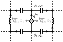
Figure 1: Example network with the loop charges $Q_{1}$ and $Q_{2}$, which are the time-integrated currents circulating in the loops in the specified orientation, and their conjugate momenta $\Phi_{1}$ and $\Phi_{2}$, which are the fluxes in the respective loops. For comparison, we also indicate node fluxes $\phi_{1}$ and $\phi_{2}$ at two nodes (shown as dots) of the network together with their conjugate momenta $q_{1}$ and $q_{2}$ which are the charges on the islands. For general networks the physical charge across a branch is related to the charges on the islands in a highly nonlocal way. In contrast, it is easy to see that using the loop charges $Q_{1}$ and $Q_{2}$, we obtain the local expression $q_{b}^{\text{br}}=Q_{1}-Q_{2}$ for the polarization charge across the phase-slip junction (diamond) taking their respective orientations into account. We have also indicated the transverse flux flow through the phase-slip junction (gray double-headed arrow). In contrast to a normal capacitor, in a phase-slip junction, the flow of flux is quantized in units of the superconducting flux quantum $\Phi_{Q}$. This expresses the duality to a Josephson junction which features longitudinal charge-transport in the direction of the element which is quantized in units of the Cooper-pair charge $2e$.

II.1 Node flux representation

The Kirchhoff voltage law states that the “vector field” $\bm{\phi}^{\text{br}}$ is conservative. Therefore the Kirchhoff voltage law can automatically be satisfied provided the fluxes $\bm{\phi}^{\text{br}}$ are represented via the “gradient” of a potential. In the discrete graph setting, the potential is given by the node fluxes $\phi_{n}$ that are placed on each node $n$ of the circuit. For a branch $b$ directed from node $n$ to node $n^{\prime}$, the branch flux $\phi^{\text{br}}_{b}$ is obtained as the discrete gradient $\phi^{\text{br}}_{b}=\phi_{n}-\phi_{n^{\prime}}$ of the node fluxes (along $b$). In this way, the node fluxes determine all the voltage drops over the branches of the circuit. Since the physical voltages depend only on differences of node fluxes, we may arbitrarily set the flux of one of the nodes (called the ground node) to zero. The voltage $\dot{\phi}_{n}$ associated with a node flux can then be interpreted as a voltage relative to ground.

The Kirchhoff current law is implemented through the equations of motion of a Lagrangian $\mathcal{L}(\bm{\phi},\dot{\bm{\phi}})$ which is constructed as follows. Each inductive element at a branch $b$ adds the term $-U(\phi_{b}^{\text{br}})$ to the Lagrangian, where

$$U(\phi_{b}^{\text{br}})=\int_{0}^{\phi_{b}^{\text{br}}(t)}\!d\phi\,f_{I,b}(\phi)$$ (5)

is simply the magnetic field energy as can be easily verified by integrating the power $V_{b}^{\text{br}}(t)I_{b}^{\text{br}}(t)$ over time and using the relation (4). Similarly, each capacitive element with capacitance $C$ adds a term $C\dot{\phi}_{b}^{2}/2$ which is just the electric field energy.

The equations of motion with respect to a node flux $\phi_{n}$ are given by the Euler-Lagrange equations

$$\frac{d}{dt}\frac{\partial\mathcal{L}}{\partial\dot{\phi}_{n}}-\frac{\partial\mathcal{L}}{\partial\phi_{n}}=0.$$ (6)

Let us consider a branch directed from a node $n^{\prime}$ towards a node $n$ such that $\phi_{b}^{\text{br}}=\phi_{n^{\prime}}-\phi_{n}$. For inductive branches, we obtain a term $-I_{b}^{\text{br}}=-f_{I,b}(\phi_{b}^{\text{br}})$ to the current balance while for capacitive branches, we obtain a term $-C\ddot{\phi}_{b}^{\text{br}}$. In both cases, this is just the current flowing away from node $n$ through branch $b$. For the opposite orientation $\phi_{b^{\prime}}^{\text{br}}=\phi_{n}-\phi_{n^{\prime}}$, we would obtain $I_{b^{\prime}}^{\text{br}}=f_{I,b^{\prime}}(\phi_{b^{\prime}}^{\text{br}})$ and $C\ddot{\phi}_{b^{\prime}}^{\text{br}}$. In both cases, we therefore obtain the current flowing away from node $n$. We conclude that the equations of motion for the node flux $\phi_{n}$ reproduce the Kirchhoff current law at node $n$. The formalism can straightforwardly be extended to include electromotive forces due to external magnetic fields, see Ref. devoret:96, .

The form of the constitutive relation (4) indicates that the node flux representation is well-suited for the description of nonlinear inductances. The knowledge of the branch flux $\phi_{b}^{\text{br}}$ over an inductance readily gives access to the voltage and the current through Eq. (4). Moreover, the terms (5) added to the Lagrangian can simply be interpreted as (possibly nonlinear) potential energy terms which pose no problem for circuit quantization.

In contrast, the node flux formulation cannot be used for the description of nonlinear capacitors. The constitutive relation (3) shows that the natural variable for a capacitor is the branch charge $q_{b}^{\text{br}}$ rather than the branch flux $\phi_{b}^{\text{br}}$. Determining the current flow through the capacitor solely from the knowledge of $\phi_{b}^{\text{br}}$ is generally impossible. Although for invertible $f_{V,b}$, we may in principle obtain $I_{b}^{\text{br}}=\ddot{\phi}_{b}^{\text{br}}/f_{V,b}^{\prime}[f_{V,b}^{-1}(\dot{\phi}_{b}^{\text{br}})]$, generating this term through the equations of motion requires adding a term of the form $\int_{0}^{\dot{\phi}_{b}^{\text{br}}}\!dV\,f^{-1}_{V,b}(V)$ to the Lagrangian. This will only lead to a quadratic kinetic energy term $C\dot{\phi}_{b}^{2}/2$ when considering a linear capacitor $C$. In contrast, a circuit containing a nonlinear capacitance cannot readily be quantized when described in terms of node fluxes $\phi_{n}$. To that end, we need a charge-based description which we will describe in details in the next section.

II.2 Loop charge representation

While the idea of representing the ‘vector field’ $\bm{\phi}^{\text{br}}$ by a ‘scalar potential’ $\bm{\phi}$ in order to guarantee the Kirchhoff voltage law is rather natural, it may be less obvious how to define charge degrees of freedom which automatically guarantee current conservation. For a planar graph that is effectively two-dimensional such that it can be drawn on a sheet of paper without crossing lines, the correct degrees of freedom for that purpose are the loop charges $Q_{l}$. They are the time-integrated loop currents circulating within every loop $l$ of the network that does not have any inner loops, c.f. Fig. 1. We give an orientation to the loop charges by specifying the orientation of a positive current flow. This orientation is in principle arbitrary but the simplest rules emerge for a consistent choice of orientation. In the current paper, we choose the orientation of all loop currents to be counter-clockwise.

Similar to the node fluxes, the loop charges are unphysical degrees of freedom in the sense that they generally do not correspond directly to a physical charge on a branch of the network. For example, by simple inspection of Fig. 1, we observe that the polarization charge $q^{\text{br}}_{b}$ of the phase-slip junction (diamond) on the branch $b$ in the specified direction is given by the difference $q^{\text{br}}_{b}=Q_{1}-Q_{2}$ of the loop charges with their indicated orientations; here, the loop charge $Q_{1}$ ($Q_{2}$) enters with a plus (minus) sign as its orientation is along (opposite) to that of $q^{\text{br}}_{b}$. While in the node flux formulation, we obtain the physical flux across every branch as the difference of node fluxes on neighboring nodes, in the loop charge formulation, we obtain in this way the physical (polarization) charge across every branch as the difference of loop charges in neighboring loops. By formally placing a loop charge $Q_{0}=0$ at the exterior of the circuit, this statement also remains correct for finite circuits with a boundary.

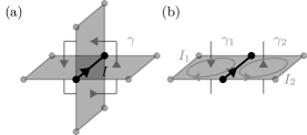
Figure 2: Motivation of loop currents from Maxwell’s equations for a lumped element circuit, represented in terms of its nodes (dots) and faces (light filled rectangles). In (a) a general network is shown with a current $I$ (dark arrow) along a directed branch of the circuit. The contour $\gamma$ (light arrows) encircles the current $I$. According to Maxwell’s equations, current conservation is guaranteed when the current $I$ running through the branch is obtained from the circulation of the magnetic field around it, $I\propto\oint_{\gamma}d\bm{s}\cdot\bm{B}$. The total current $I$ can be decomposed into a sum of currents $I_{l}\propto\int_{\gamma_{i}}d\bm{s}\cdot\bm{B}$, where each part $\gamma_{l}$ of the contour is associated with a specific face of the circuit graph that is pierced by the contour. The currents $I_{l}$ have a direct interpretation in terms of the currents circulating around the pierced loops. This is particularly easy to see for a planar circuit depicted in (b) as we may close the contour integral at infinity. As a result, we obtain $I=(-I_{1})-I_{2}$, in line with the interpretation of the currents $I_{l}$ as currents circulating in loop $l$. Viewing the circuit from above, we recover Fig. 1.

The loop charge construction can also be justified directly from Maxwell’s equations. According to Maxwell’s equations, current conservation (in a stationary situation) is guaranteed when the current $I$ flowing through some area bounded by a contour $\gamma$ is obtained from the circulation of the magnetic field according to $I\propto\oint_{\gamma}d\bm{s}\cdot\bm{B}$. For each branch $b$ of the network, we can decompose the current $I_{b}$ into a sum of currents $I_{l}\propto\int_{\gamma_{l}}d\bm{s}\cdot\bm{B}$, where each part $\gamma_{l}$ of the contour is associated with a specific face of the circuit that is pierced by the contour, see Fig. 2(a). The current $I_{l}$ can be interpreted as the loop current within the pierced loop $l$, see Fig. 2(b). The loop charge $Q_{l}$ is then simply related to the current $I_{l}$ as $\dot{Q}_{l}=I_{l}$. The above considerations also show that we will generally only obtain the current from the difference of precisely two loop charges when the circuit is planar, i.e., effectively two-dimensional thulasiraman . We show in App. A that the loop charge description is indeed limited to planar circuits.

Figure 3: The left column depicts various circuit elements [inductor $L$, capacitor $C$, mutual inductance $M$, general capacitance with voltage-charge relation $V=f_{V}(Q)$, voltage source $V$, and external flux $\Phi^{\text{ex}}$] with their corresponding expression in the Lagrangian (right column). In a planar graph, each of the circuit elements is part of two loops with loop charges $Q_{1}$ and $Q_{2}$ which are indicated along with their respective orientation for completeness. The simplest representation of a phase-slip junction amounts to choosing $f_{V}(Q)=(\pi E_{S}/e)\sin(\pi Q/e)$, where $E_{S}/\hbar$ is the phase-slip rate. This corresponds to a term $E_{S}\cos[\pi(Q_{1}-Q_{2})/e]$ in the Lagrangian.

Having identified the loop charges $\bm{Q}$ as variables guaranteeing current conservation, we are left with the task of defining a Lagrangian whose equations of motion guarantee the Kirchhoff voltage law. The construction of this Lagrangian is analogous to the construction of the Lagrangian for the node fluxes. Specifically, each capacitive element adds a term $-U(q_{b}^{\text{br}})$ to the Lagrangian, where

$$U(q_{b}^{\text{br}})=\int_{0}^{q_{b}^{\text{br}}(t)}\!dq\,f_{V,b}(q)$$ (7)

is just the electric energy stored in the capacitor. Specifically, for the simplest model $f_{V}(Q)=V_{c}\sin(\pi Q/e)$ of a phase-slip junction, we obtain the term (up to a constant)

$$U(q_{b}^{\text{br}})=-E_{S}\cos(\pi q_{b}^{\text{br}}/e)$$ (8)

with the characteristic energy $E_{S}=eV_{c}/\pi$. For each linear inductor $L$, we add a kinetic term of the form $L(\dot{q}_{b}^{\text{br}})^{2}/2$. In this way, the equations of motion with respect to a loop charge $Q_{l}$ yield the balance of voltage drops obtained from a counter-clockwise traversal of the loop $l$. The relevant terms that have to be added to the Lagrangian are summarized for different components in Fig. 3. Since Josephson junctions are nonlinear inductors, they cannot be directly described using the loop charge formulation. We will introduce a way to obtain a charge-based descriptions of Josephson junctions in Sec. VI (see also the comments in Sec. III.1).

A Hamiltonian description requires the introduction of canonical momenta

$$\Phi_{l}=\partial\mathcal{L}/\partial{\dot{Q}_{l}}.$$ (9)

Each $\Phi_{l}$ can be interpreted as the loop flux in the loop $l$ of the circuit. If the relation (9) between the loop fluxes $\bm{\Phi}$ and the loop charges $\bm{Q}$ is invertible, we can perform the Legendre transformation

$$H=\bm{\Phi}\cdot\dot{\bm{Q}}-\mathcal{L}(\bm{Q},\dot{\bm{Q}})$$ (10)

and obtain the circuit Hamiltonian which can be readily quantized through the introduction of canonical commutation relations $[\Phi_{j},Q_{k}]=\delta_{jk}i\hbar$.

It may happen that the relation (9) between the loop charges $\bm{Q}$ and the conjugate momenta $\bm{\Phi}$ is not invertible. This indicates that not all loop currents are dynamical degrees of freedom. A simple example for this is an inductor $L$ with two parallel capacitances $C_{1}$ and $C_{2}$ to the left and the right. Denoting the loop charges in the two loops by $Q_{1}$ and $Q_{2}$, the corresponding Lagrangian reads $\mathcal{L}=L(\dot{Q}_{1}-\dot{Q}_{2})^{2}/2-Q_{1}^{2}/2C_{1}-Q_{2}^{2}/2C_{2}$. Introducing $Q=Q_{1}-Q_{2}$ and $Q^{\prime}=(Q_{1}+Q_{2})/2$, it is obvious that the state of the system depends only on the current $\dot{Q}$ through the inductor and not on the currents through the capacitive branches. As a consequence, the Lagrangian does not depend on $\dot{Q}^{\prime}$ which gives the constraint $\partial\mathcal{L}/\partial\dot{Q}^{\prime}=0=\Phi^{\prime}$ for the momentum $\Phi^{\prime}$ conjugate to $Q^{\prime}$ which cannot be solved for $\dot{Q}^{\prime}$. However, the fact that the Lagrangian does not depend on $\dot{Q}^{\prime}$ also means that the Euler-Lagrange equations for $Q^{\prime}$ are purely algebraic equations (constraints) which can be solved immediately. Resolving the constraint for $Q^{\prime}$ and reinserting the solution into the Lagrangian yields the regular Lagrangian $\mathcal{L}=L\dot{Q}^{2}/2-Q^{2}/2(C_{1}+C_{2})$. Resolving all constraints in such a way in general leads to a reduced Lagrangian involving only dynamical degrees of freedom such that the Legendre transformation (10) and quantization can be performed.

Superconducting circuits with Josephson junctions or phase-slip junctions may involve transport of strictly quantized charges or fluxes through the circuit. The former situation occurs when a superconducting island is connected to the rest of the network only by capacitors and Josephson junctions. The isolation of the island demands that the node charge $q_{n}$ of the island is quantized in units of $2e$ which corresponds to a $\Phi_{Q}$-periodicity of the wavefunction in terms of the node flux $\phi_{n}$. The latter situation occurs if a loop $l$ involves only inductors and phase-slip junctions. In this case the flux $\Phi_{l}$ in the loop is quantized in units of $\Phi_{Q}$ corresponding to a $2e$-periodicity of the wavefunction with respect to the corresponding loop charge $Q_{l}$.

Instead of focusing on the circuit to identify islands with integer node charges (in units of $2e$) or loops with integer loop fluxes (in units of $\Phi_{Q}$) to determine the appropriate boundary conditions for the quantization of the fluxes or charges, we may also determine the appropriate choice of boundary conditions by looking at the symmetries of the Hamiltonian. The quantization of fluxes or charges is due to the periodicity of the underlying potentials. If one ignores the periodicity considerations of the wavefunction as described above and works with node fluxes $\bm{\phi}$ or loop charges $\bm{Q}$ defined on the entire real axis, the periodicity leads to the existence of conserved quantities which correspond to Bloch quasi-momenta. A specific choice of Bloch momentum then corresponds to a choice of initial condition. Due to the relations (1) and (2), our inital condition for $t\to-\infty$ corresponds to a charge- and flux-less state and thus all the Bloch momenta vanish (implying periodic wave-functions). The two approaches are therefore equivalent and one may choose whatever method seems more convenient. The symmetry-based perspective will be particularly useful in the mixed formulation to be discussed in Sec. V.

A typical lumped element circuit does not just involve passive elements like capacitors and inductors, but also involves active elements like voltage and current sources. It will also feature electromotive forces due to time-varying fluxes or offset charges on some island of the network. Voltage sources generating a voltage drop $V_{i}^{\text{ex}}$ are easily described by adding a term $-q_{i}^{\text{br}}V_{i}^{\text{ex}}$ to the Lagrangian, where $q_{i}^{\text{br}}$ is the corresponding branch charge expressed in terms of the loop charges. Similarly, for a loop $l$ with loop charge $Q_{l}$ and external flux $\Phi^{\text{ex}}_{l}$ which generates a positive voltage drop $V=\dot{\Phi}^{\text{ex}}_{l}$ in the loop current direction, a term $\dot{Q}_{l}\Phi^{\text{ex}}_{l}$ should be added to the Lagrangian.

Offset charges are slightly more difficult to handle since they modify the current balance rather than the voltage balance. This means that they cannot be described in terms of loop charges with the simple rules given in Sec. II.2 since no term added to the equations of motion can modify the current balance. Instead, one must represent them through additional branches which are described in terms of node fluxes. This requires a mixed loop charge/node flux formulation that we will describe in detail in Sec. V. In the end, however, we obtain a simple rule that we will state now for convenience and whose proof we defer to Sec. V. To understand the rule, we first note that the lumped element description requires overall charge neutrality since otherwise there is a net electric field that extends through the circuit and is not confined to the lumped elements. This means that we can only specify $n-1$ offset charges $q^{\text{ex}}_{i}$ with $i\neq 0$ on the $n$ islands of the circuit since overall neutrality implies that the offset charges leave behind a charge $q_{0}^{\text{ex}}=-\sum_{i\neq 0}q_{i}^{\text{ex}}$ on the ground node with $i=0$.

Figure 4: Example network consisting of 6 branches $b_{1},\dots,b_{6}$ and $5$ nodes $0,\dots,4$. If the branches $b_{4}$ and $b_{6}$ (thin lines) are removed from the graph, the branches $b_{1},b_{2},b_{3},b_{5}$ (thick lines) still connect all nodes and therefore form a spanning tree of the graph. Choosing the node $0$ as the ground node, we can only specify the offset charges $q_{1}^{\text{ex}},\dots,q_{4}^{\text{ex}}$ on the remaining nodes since the ground node must carry the charge $q_{0}^{\text{ex}}=-\sum_{i=1}^{4}q_{i}^{\text{ex}}$ to guarantee overall charge neutrality. As explained in the main text, in order to accommodate the offset charges in our circuit description, we have to determine which offset charges are transported through which tree branches on their way from the ground to their respective node. For example, the offset charge $q_{2}^{\text{ex}}$ has to be transported along the tree branches $b_{1}$, $b_{2}$ and $b_{5}$ in order to arrive at node $2$.

In order to handle the offset charges $q_{i}^{\text{ex}}$, one must consistently keep track of the paths through which the polarization charge propagates on its way from the ground node to node $i$. To that end, we use the concept of a spanning tree. For a graph, a spanning tree is defined as a subgraph which does not have any loops and connects all nodes. The branches of the graph that belong to the spanning tree are called tree branches. Since a spanning tree of a connected graph with $n$ nodes has $n-1$ tree branches, we obtain a one-to-one relation between the $n-1$ tree branches and the $n-1$ offset charges.

The offset charges can now be included following a number of simple steps. We first choose a ground node and construct a spanning tree of the circuit. In a second step, we express the branch charges $\bm{q}^{\text{br}}$ of the circuit as differences of loop charges, following the same reasoning that we apply in absence of offset charges. As a last step, for all tree branches $b$, we shift the resulting charge expression $q^{\text{br}}_{b}$ by replacing $q^{\text{br}}_{b}\mapsto q^{\text{br}}_{b}\pm\Sigma^{\text{ex}}_{b}$. We use the plus sign if the branch $b$ is directed away from the ground node and the minus sign otherwise. The sum $\Sigma^{\text{ex}}_{b}$ is the sum of all the external offset charges $q^{\text{ex}}_{i}$ that have passed through the tree branch $b$ on their unique way from the ground node to node $i$ (within the tree). Note that the specific choice of spanning tree is a gauge in the sense that it has no physical consequences. It only amounts to a redefinition of the meaning of the charges $\bm{q}^{\text{br}}_{b}$ that no longer give the physical charge on the respective tree element.

As an example, consider the capacitive network depicted in Fig. 4 consisting of six branches $b_{1},\dots,b_{6}$ and 5 nodes $0,\dots,4$ with respective offset charges $q_{1}^{\text{ex}},\dots,q_{4}^{\text{ex}}$. As a first step, we choose the node $0$ as the ground node and use a spanning tree consisting of the branches $b_{1}$, $b_{2}$, $b_{3}$, and $b_{5}$ (thick lines). For the next steps, let us explicitly consider the branch $b_{1}$. In absence of offset charges, the branch charge $q_{1}^{\text{br}}$ can be expressed as $q_{1}^{\text{br}}=-Q_{1}$ in terms of loop charges. Next we determine $\Sigma_{1}^{\text{ex}}$. Since the offset charges $q_{1}^{\text{ex}}$, $q_{2}^{\text{ex}}$, $q_{3}^{\text{ex}}$, and $q_{4}^{\text{ex}}$ all have to pass through the branch $b_{1}$ in order to reach their respective nodes while traversing only tree branches, we find $\Sigma_{1}^{\text{ex}}=\sum_{i=1}^{4}q_{i}^{\text{ex}}$. Since $b_{1}$ is directed away from the ground node, including the offset charges amounts to the replacement $q_{1}^{\text{br}}=-Q_{1}\mapsto-Q_{1}+\Sigma_{1}^{\text{ex}}$. Proceeding in a similar way with the other branches, we obtain the Lagrangian

$$\mathcal{L} ={-}\frac{(q_{1}^{\text{ex}}{+}q_{2}^{\text{ex}}{+}q_{3}^{\text{ex}}{+}q_{4}^{\text{ex}}{-}Q_{1})^{2}}{2C_{1}}-\frac{(Q_{1}{-}q_{2}^{\text{ex}}{-}q_{3}^{\text{ex}}{-}q_{4}^{\text{ex}})^{2}}{2C_{2}}$$

$$-\frac{(q_{4}^{\text{ex}}{-}Q_{2})^{2}}{2C_{3}}-\frac{Q_{2}^{2}}{2C_{4}}-\frac{(q_{2}^{\text{ex}}{+}Q_{2}{-}Q_{1})^{2}}{2C_{5}}-\frac{Q_{1}^{2}}{2C_{6}}.$$ (11)

We note that in line with our previous discussion, the charge expressions of the branches $b_{4}$ and $b_{6}$ which do not belong to the tree have not been modified by the offset charges.

With the offset charge description, we can simply represent a current source, which injects a current $I^{\text{ex}}$ into the circuit and points from node $n$ to node $n^{\prime}$ by adding the offset charge $\int^{t}dt^{\prime}I^{\text{ex}}(t^{\prime})$ at node $n^{\prime}$ and the offset charge $-\int^{t}dt^{\prime}I^{\text{ex}}(t^{\prime})$ at node $n$.

III Duality between node fluxes and loop charges

In the previous section, we have discussed two representations of the Lagrangian of a circuit, one in terms of node fluxes and the other in terms of loop charges. In the following, we will call such a change in description of the same system from node fluxes to loop charges a passive duality transformation. Besides those passive duality transformations of the same circuit, one can also consider active duality transformations which yield a different, electromagnetically dual circuit whose charge dynamics is identical to the flux dynamics of the original circuit or vice-versa. Electromagnetic circuit dualities have been discussed on a per-case basis in the mesoscopic physics literature mooij:06 ; guichard:10 ; kerman:13 but, to our knowledge, a general construction scheme has not been spelled out so far.

In this section, we will explain how to explicitly construct both passive and active duality transformations with the help of loop charges. We will start by discussing the explicit construction of passive duality transformations. Previously, we have focused on the question on how to read off the appropriate Lagrangian in either representation directly from a given circuit graph. We now show how one can transform one representation into the other. While this is of technical interest, we want to highlight that this subsection may be skipped on first reading since in practice it is sufficient and much easier to use the rules given in Sec. II.2 for the construction of the loop charge Lagrangian. We proceed by outlining in Sec. III.2 a straightforward way of constructing electromagnetic circuit dualities using loop charges.

III.1 Passive duality transformations

The transformation from the node flux to a loop charge representation is particularly easy to perform in the path integral picture hibbs . In this case, the unitary time-evolution operator $e^{-iHt/\hbar}$ is represented in the form

$$e^{-iHt/\hbar}\rightarrow\int\!\mathcal{D}[\bm{\phi}(t)]\,e^{(i/\hbar)\int^{t}\!dt^{\prime}\,\mathcal{L}(\bm{\phi}^{\text{br}})},$$ (12)

where the path-integration is performed over the $n-1$ node fluxes of the circuit graph with $n$ nodes. Note that we have also suppressed the dependence of the Lagrangian on $\dot{\bm{\phi}}^{\text{br}}$ for brevity. The description in terms of branch fluxes $\bm{\phi}^{\text{br}}$ is linked to a description in terms of branch charges $q_{b}^{\text{br}}=\partial\mathcal{L}(\bm{\phi}^{\text{br}},\dot{\bm{\phi}}^{\text{br}})/\partial\dot{\phi}_{b}^{\text{br}}$ through the Legendre transformation. For the following, it will be convenient to perform this Legendre transformation in a slightly more general form through the Fourier transformation

$$e^{(i/\hbar)\int^{t}\!dt^{\prime}\,\mathcal{L}(\bm{\phi}^{\text{br}})}=\int\!\mathcal{D}[\bm{q}^{\text{br}}(t)]e^{(i/\hbar)\int^{t}\!dt^{\prime}[\tilde{\mathcal{L}}(\bm{q}^{\text{br}})-\bm{q}^{\text{br}}\cdot\dot{\bm{\phi}}^{\text{br}}]},$$ (13)

where the Lagrangian $\tilde{\mathcal{L}}(\bm{q}^{\text{br}},\dot{\bm{q}}^{\text{br}})$ is defined implicitly such that Eq. (13) holds. At the saddle-point level or for a Lagrangian $\tilde{\mathcal{L}}(\bm{q}^{\text{br}},\dot{\bm{q}}^{\text{br}})$ that is quadratic in its arguments, performing the $\bm{q}^{\text{br}}$ integration shows that $\mathcal{L}(\bm{\phi}^{\text{br}},\dot{\bm{\phi}}^{\text{br}})$ is simply the Legendre transformation of $\tilde{\mathcal{L}}(\bm{q}^{\text{br}},\dot{\bm{q}}^{\text{br}})$.

To proceed further, we need to relate the node fluxes $\bm{\phi}$ to the branch fluxes $\bm{\phi}^{\text{br}}$. For this, we make use of the basis node-edge incidence matrix $A$ which is a $\mathbb{R}^{(n-1)\times b}$ matrix for the $n-1$ nodes fluxes and the $b$ branches. Its entries $A_{ij}\in\{1,-1\}$ indicate whether the branch $j$ enters ($-1$) or leaves $(+1)$ node $i$. It allows us to express the Kirchhoff current law in the form $A\dot{\bm{q}}^{\text{br}}=0$ and it relates the branch and node fluxes via $\bm{\phi}^{\text{br}}=A^{T}\bm{\phi}$.

Performing a partial integration on the term $-\bm{q}^{\text{br}}\cdot\dot{\bm{\phi}}^{\text{br}}=-\bm{q}^{\text{br}}\cdot A^{T}\dot{\bm{\phi}}$ in the exponent of expression (13), inserting the resulting expression into Eq. (12), and performing the integration over $\bm{\phi}$ results in a constraint:

$$e^{-iHt/\hbar}\rightarrow\int\!\mathcal{D}[\bm{q}^{\text{br}}(t)]e^{(i/\hbar)\int^{t}\!dt^{\prime}\,\tilde{\mathcal{L}}(\bm{q}^{\text{br}})}\delta[A\dot{\bm{q}}^{\text{br}}(t)],$$ (14)

where the $\delta$ function has to be understood in such a way that it demands the vanishing of its argument at each point in time. The constraint $A\dot{\bm{q}}^{\text{br}}=0$ is of course nothing but the Kirchhoff current law. As we have discussed in details in Sec. II.2, we can guarantee the Kirchhoff current law for a planar circuit by considering loop charges. This resolves the constraint and we obtain the dual representation

$$e^{-iHt/\hbar}\rightarrow\int\!\mathcal{D}[\bm{Q}(t)]e^{(i/\hbar)\int^{t}\!dt^{\prime}\,\tilde{\mathcal{L}}[\bm{q}^{\text{br}}(\bm{Q})]}$$ (15)

in terms of loop charges. For the convenience of the reader, we repeat this derivation in a slightly more rigorous way in App. B.

We have thus explicitly constructed the passive duality transformation linking a representation in terms of node fluxes to a representation in terms of loop charges. We want to stress once again that in practice it is much easier and much less error-prone to perform the construction of the circuit Lagrangian using the rules explained in details in Sec. II.2, rather than starting with a node-flux representation and repeating the calculation outlined above.

It is interesting to note that the duality transformation used here is essentially the same as the one used in the analysis of the classical two-dimensional XY-model savit:80 or the Schmid-Bulgadaev transition. In fact, the analogy to the XY-model suggests that Josephson junctions can be described in the loop charge formulation by making the Villain approximation for the cosine dispersion $E_{J}\cos(2\pi\phi^{\text{br}}/\Phi_{Q})$ of a Josephson junction with branch flux $\phi^{\text{br}}$. There, one replaces the cosine dispersion by the function $-\min_{m\in\mathbb{Z}}E_{J}(2\pi\phi^{\text{br}}/\Phi_{Q}-2\pi m)^{2}/2$ which retains the $\Phi_{Q}$ periodicity while being quadratic in $\phi^{\text{br}}$. This allows to perform the path integration over $\bm{\phi}$ and construct a charge-based description of a Josephson junction in the Villain approximation. We will not pursue this idea further since we will introduce in Sec. VI an alternative way to describe a Josephson junction (using loop charges) that is based on the adiabatic separation of the (fast) Cooper-pair transport through the junction and the (slow) transport of polarization charge through the rest of the circuit.

III.2 Active duality transformations: electromagnetic circuit duality

In the previous section, we have explained the representations of circuits in terms of node fluxes or loop charges which are related by a passive duality transformation. We now want to show that loop charges are also useful for constructing active duality transformations. Specifically, given a graph $g$ of a circuit that is described in terms of node fluxes and has a corresponding Lagrangian $\mathcal{L}(\bm{\phi},\dot{\bm{\phi}})$, we define its electromagnetically dual circuit with graph $G$ as the circuit whose description in terms of loop charges yields a Lagrangian that is of the same form as $\mathcal{L}(\bm{\phi},\dot{\bm{\phi}})$ with $\bm{\phi}$ replaced by a vector of loop charges $\bm{Q}$. We will see below that a dual circuit exists for planar circuits which are effectively two-dimensional such that the closure of flux lines in the third dimension can be ignored; this is in contrast to classical electromagnetism where electromagnetic dualities only exist in vacuum due to the absence of magnetic monopoles jackson .

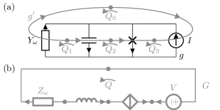
Figure 5: In (a), we illustrate the construction of the graph $g^{\prime}$ dual to a graph $g$. As explained in the main text, we construct $g^{\prime}$ by placing one node into each loop of $g$. We connect two nodes in the dual graph $g^{\prime}$ whenever there is a circuit element on branch $b$ in $g$ that separates the corresponding loops $l_{0}$ and $l_{1}$. The orientation on the branch in $g^{\prime}$ is chosen such that the branch points towards $l_{1}$ if the orientation of the loop charge $Q_{l_{1}}$ is consistent with the orientation of the original branch in $g$ and away from $l_{1}$ otherwise. In (b), we show the electromagnetic dual graph $G$ that is obtained from $g^{\prime}$ by replacing the elements according to the rules given in Fig. 1.

In order to construct the dual circuit $G$, we first need the notion of a dual graph $g^{\prime}$. In the node flux formulation, each branch flux $\phi^{\text{br}}_{b}$ is obtained as the difference of precisely two node fluxes. We have seen previously that for a planar circuit described in terms of loop charges, we can similarly describe each branch charge $q^{\text{br}}_{b}$ as the difference of two loop charges, provided we also place a loop charge $Q_{0}=0$ at the exterior of the circuit. For this reason, we construct the dual graph $g^{\prime}$ by placing one node into each loop of the original graph $g$, including the “loop” at the exterior Note2 . For each branch $b$ representing a circuit element that is common to the loops $l_{0}$ and $l_{1}$, we add a branch $b^{\prime}$ in the dual graph representing the same circuit element that joins the dual nodes at $l_{0}$ and $l_{1}$. We choose the orientation of the dual branch such that it points towards $l_{1}$ if the orientation of the original branch is consistent with the loop charge orientation $Q_{l_{1}}$ and away from $l_{1}$ otherwise. This gives a consistent scheme provided we choose a counter-clockwise orientation for all loop charges as described in Sec. II.2. The construction scheme is illustrated in Fig. 5(a) for a simple circuit. Associating the loop charges of the original circuit with the nodes of the dual graph, the charge on branch $b$ of the original circuit can be obtained as the negative (discrete) gradient of the loop charges along the branch $b^{\prime}$ of the dual graph. Up to a sign, we thus obtain the branch charge $q_{b}$ of the original graph $g$ from the dual graph $g^{\prime}$ in a way that is completely analogous to the node flux formulation. Note that the dual graph does not represent a lumped element representation of a physical circuit but it should rather be considered a handy mnemonic for the loop charge representation of the original circuit. We highlight that iterating this procedure twice gives back the original graph with the orientation of all branches reversed.

To construct the dual circuit $G$, we start by considering the dual graph $g^{\prime}$ of $g$ as a lumped element representation of an actual circuit different from the original circuit. As we have explained before, we can understand the loop charge formulation of $g^{\prime}$ by thinking about the loop charges of $g^{\prime}$ sitting on the nodes of $(g^{\prime})^{\prime}$. Now, since $(g^{\prime})^{\prime}$ is just the original graph $g$ with all branch orientations reversed, we effectively obtain the branch charges of $g^{\prime}$ as the gradient of the loop charges positioned on the nodes of the original graph $g$. Thus, we obtain the result that the node fluxes of $g$ are in one to one relation with the loop charges of $g^{\prime}$. From $g^{\prime}$, we obtain the dual circuit $G$ by replacing circuit elements of $g^{\prime}$ in such a way that the loop charges of $G$ have the same dynamics as the node fluxes of $g$. In order to have the same dynamics, the terms in the Lagrangian corresponding to the circuit elements have to be equal (up to interchanging $\bm{\varphi}$ with $\bm{Q}$). For example, a capacitive element in $g$ corresponds to a (kinetic) term of the form $C\dot{\phi}^{2}/2$ and its dual is thus given by an inductor $L\dot{Q}^{2}/2$ (which leads to a kinetic term in the loop charge description). More generally, we obtain the electromagnetically dual circuit $G$ from the dual graph $g^{\prime}$ of $g$ by replacing all elements in $g^{\prime}$ according to the rules given in Table 1. This procedure is illustrated in Fig. 5(b) for a simple circuit.

Original		Dual
Capacitance $C$		Inductance $L$
Josephson junction $E_{J}$		Phase-slip junction $E_{S}$
Flux $\phi^{\text{ex}}$ through loop $n$		Offset charge $q^{\text{ex}}$ at node $n$
Voltage source $V$		Current source $I$
Admittance $Y_{\omega}$		Impedance $Z_{\omega}$

Table 1: Circuit elements and their corresponding elements in the electromagnetically dual circuit.

IV Dissipation and environments

So far, we have analyzed closed systems where the energy is conserved. We have given a recipe to calculate the Lagrangian $\mathcal{L}(\bm{Q},\dot{\bm{Q}})$ that corresponds to a specific lumped-element circuit. In a typical application, we would then go on by introducing the Hamiltonian and canonically quantizing position $\bm{Q}$ and momentum $\bm{\Phi}=\partial_{\dot{\bm{Q}}}\mathcal{L}$. Given an initial configuration $\Psi_{t_{0}}(\bm{Q})$, we obtain a wavefunction $\Psi_{t}(\bm{Q})$ that describes the evolution of the probabilities $|\Psi_{t}(\bm{Q})|^{2}$ to find the system in a specific state $\bm{Q}$ at time $t$.

An altogether different but equivalent approach is the path integral method hibbs , which we already briefly discussed in Sec. III.1. There the wavefunction is obtained by the expression

$$\Psi_{t}(\bm{Q})=\int\!\mathcal{D}[\bm{Q}(t)]e^{(i/\hbar)\int_{t_{0}}^{t}\!dt^{\prime}\,\mathcal{L}}\,\Psi_{t_{0}}(\bm{Q}^{\prime})$$ (16)

that sums over all paths $\bm{Q}(t)$ fulfilling the boundary conditions $\bm{Q}(t_{0})=\bm{Q}^{\prime}$ and $\bm{Q}(t)=\bm{Q}$. Note that in this approach there is neither a need to go over to a Hamiltonian nor to postulate canonical quantization rules.

In conventional electronics, there are elements called resistors that do not conserve energy. In a quantum setting, this corresponds to open systems, i.e., a system coupled to an environment; an example is an electronic circuit which is coupled to the outside via a electromagnetic transmission line. We note that recently there has been a lot of progress in quantizing general linear environments in terms of a few relevant degrees of freedom nigg:12 ; bourassa:12 ; leib:12 ; solgun:14 ; solgun:15 . Here, we will describe the environment as an effective action on the system degrees of freedom.

In the theory of open systems, the interest is in characterizing the system in questions without having to specify the full wavefunction of the system together with its environment. As in this case the system does not stay in a pure state, it necessarily has to be characterized by its density matrix $\rho_{t}(\bm{Q}^{+},\bm{Q}^{-})$ whose diagonal elements give the probability to observe the system in a particular state $\bm{Q}^{-}=\bm{Q}^{+}$ and the off-diagonal terms characterize the coherences. We see that the fact that the system is open requires to double the degrees of freedom, i.e., going from $\bm{Q}$ to $\bm{Q}^{\pm}$. The dynamics of the system is simply given by

$$\rho_{t}(\bm{Q}^{+},\bm{Q}^{-})=\int\!\mathcal{D}[\bm{Q}^{+}(t),\bm{Q}^{-}(t)]e^{i\mathcal{S}/\hbar}\,\rho_{t_{0}}(\bm{Q}^{\prime+},\bm{Q}^{\prime-})$$ (17)

where $\mathcal{S}=\mathcal{S}_{S}+\mathcal{S}_{E}$ has a contribution due to the system (without the environment)

$$\mathcal{S}_{S}=\int_{t_{0}}^{t}\!dt^{\prime}[\mathcal{L}(\bm{Q}^{+},\dot{\bm{Q}}^{+},t)-\mathcal{L}(\bm{Q}^{-},\dot{\bm{Q}}^{-},t)].$$ (18)

The influence of the environment can be captured by the so-called influence functional $\mathcal{S}_{E}$ feynman:63 .

If the environment is a linear system in equilibrium characterized by the impedance $Z_{\omega}$, the influence functional can be calculated explicitly caldeira:83 ; schon:90 . If the branch $b$ (between the two loops $l_{0}$ and $l_{1}$) with branch charge $q^{\text{br}}_{b}=Q_{l_{1}}-Q_{l_{0}}$ is shunted by the impedance $Z_{\omega}$, we obtain the additional action $\mathcal{S}_{E}=\mathcal{S}_{R}+\mathcal{S}_{D}$ with a reactive part

$$\mathcal{S}_{R}=\int\!\frac{d\omega}{4\pi}\mathop{\rm Im}(Z_{\omega})\,\omega\Bigl{(}|\tilde{Q}^{-}_{\omega}|^{2}-|\tilde{Q}^{+}_{\omega}|^{2}\Bigr{)}$$ (19)

where the Fourier-transform $\tilde{Q}^{\pm}_{\omega}=\int_{t_{0}}^{t}\!dt^{\prime}\,q^{\text{br},\pm}_{b}(t^{\prime})e^{i\omega t^{\prime}}$ enters. Note that in the reactive part, similar to the system, the variables $\tilde{Q}^{+}$ and $\tilde{Q}^{-}$ are not coupled which corresponds to the fact that the evolution of the ket and bra in a pure state $\rho_{t}=\Psi_{t}(\bm{Q}^{+})\Psi^{*}_{t}(\bm{Q}^{-})$ are independent of each other. In particular, for a simple inductance $L$ with impedance $Z_{\omega}=-i\omega L$ or a capacitance $C$ with impedance $Z_{\omega}=i/\omega C$, the expression (19) reproduces the results of Fig. 3.

The dissipation destroys this factorization and makes the doubling of the degrees of freedom inevitable. In fact, it is useful to introduce new variables $\tilde{Q}^{\text{cl}}_{\omega}=\tfrac{1}{2}(\tilde{Q}^{+}_{\omega}+\tilde{Q}^{-}_{\omega})$ and $\tilde{Q}^{q}_{\omega}=\tilde{Q}^{+}_{\omega}-\tilde{Q}^{-}_{\omega}$ in terms of which the dissipative part of the action reads

$$\mathcal{S}_{D}=\int\!\frac{d\omega}{2\pi}\mathop{\rm Re}(Z_{\omega})\,\omega\Bigl{[}\mathop{\rm Im}(\tilde{Q}^{\text{cl}}_{-\omega}\tilde{Q}^{q}_{\omega})+i(2n_{\omega}+1)|\tilde{Q}^{q}_{\omega}|^{2}\Bigr{]};$$ (20)

here, $n_{\omega}$ denotes the occupation probability of the mode at frequency $\omega$ in the environment. In particular, in equilibrium, we have the Bose-Einstein distribution $n_{\omega}={(e^{\hbar\omega/k_{B}T}-1)}^{-1}$. The two terms in (20) have different tasks: the first term introduces dissipation in the equation of motion and the last term leads to fluctuations, see also below.

As an example, we would like to analyze a setup where a phase-slip junction in series with an inductor and a resistance is voltage biased at voltage $V_{0}$, which is illustrated in Fig. 5(b). The circuit consists of a single loop with loop charge $Q$. This system is the dual of the resistively-shunted Josephson junction shown in Fig. 5(a).tinkham The Lagrangian assumes the form

$$\mathcal{L}=\frac{L\dot{Q}^{2}}{2}+E_{S}\cos(\pi Q/e)+V_{0}Q$$ (21)

involving both the phase-slip junction as well as the voltage bias. The action of the system is obtained via (18). The Ohmic resistance is modelled by dissipative action (20) with $\mathop{\rm Re}(Z_{\omega})=R$.

How the system dynamics is modified by dissipation depends on temperature. Let us first consider the case $T=0$, which can be analyzed using the well-known results for the dual problem of the resistively-shunted Josephson junction. For the following, we consider the case $V_{0}=0$. It is then advantageous to decompose the total flux within the loop in the form $\phi+\Phi$ with $\phi\in[0,\Phi_{Q}]$ and $\Phi/\Phi_{Q}\in\mathbb{Z}$. The former flux can be interpreted as the Bloch momentum associated with the dynamics of $Q$ in the $2e$-periodic potential due to the phase-slip junction, while the latter is connected to the dynamics within a single unit cell of size $2e$. For zero shunt resistance, $R=0$, the flux $\phi$ (Bloch momentum) is conserved, corresponding to a complete delocalization of $Q$ over the valleys of the cosine potential. Localizing the charge $Q$ in a single valley of the periodic potential requires a superposition of all Bloch momenta $\phi$. The fluctuation-dissipation theorem, $S_{\phi}(\omega)\propto\operatorname{Re}(Z_{\omega})$, shows that increasing $\operatorname{Re}(Z_{\omega})$ will increase the fluctuations of $\phi$ at frequency $\omega$ as described by the spectral density $S_{\phi}(\omega)=\int\!dt\,e^{i\omega t}\langle\phi(t)\phi(0)\rangle$. This suggests that for $R$ sufficiently large such that the fluctuations of $\phi$ exceed $\Phi_{Q}$, $Q$ will eventually localize within a single valley of the periodic potential. The transition from a state delocalized over different valleys of the periodic potential to a localized state is known as the Schmid-Bulgadaev quantum phase transition that was mainly studied in the dual problem of the resistively shunted Josephson junction (for zero current bias) schmid:83 ; bulgadaev:84 ; guinea:85 ; schon:90 . Translated to our problem, the results imply that $Q$ is localized for $R>R_{Q}$ and remains delocalized for $R<R_{Q}$.

For finite temperature $T$, the Schmid-Bulgadaev transition is formally absent because thermal activation will always lead to a finite probability for the charge $Q$ to transition between different valleys of the potential schon:90 . However, as long as we are on the insulating side of the Schmid transition with $R>R_{Q}$ where quantum tunneling of $Q$ is absent, we can describe the dynamics of $Q$ semi-classically. This corresponds to expanding the action around $Q^{q}=0$ kamenev , which leads to

$$\mathcal{S}=\int_{t_{0}}^{t}\!dt^{\prime}[V_{0}-L\ddot{Q}^{\text{cl}}-R\dot{Q}^{\text{cl}}-V_{c}\sin(\pi Q^{\text{cl}}/e)]Q^{q}\\ +iR\int\!\frac{d\omega}{2\pi}\omega(2n_{\omega}+1)|Q_{\omega}^{q}|^{2}$$ (22)

with $V_{c}=\pi E_{S}/e$. Next, we introduce the fluctuation $\xi$ of the voltage over the resistor via a Hubbard-Stratonovich transformation. In fact, we have that

$$e^{i\mathcal{S}_{D}}=\int\!\mathcal{D}[\xi(t)]\exp\biggl{[}-\!\int\!\frac{d\omega}{2\pi}\Bigl{(}i\xi^{*}_{\omega}Q^{q}_{\omega}+\frac{|\xi_{\omega}|^{2}}{4R\omega(2n_{\omega}+1)}\Bigr{)}\biggr{]}.$$ (23)

After this transformation, the action is linear in $Q^{q}$ which allows for performing the path-integral over $Q^{q}$. The result is the Langevin equation

$$V_{0}-L\ddot{Q}^{\text{cl}}-R\dot{Q}^{\text{cl}}-V_{c}\sin(\pi Q^{\text{cl}}/e)=\xi(t)$$ (24)

for $Q^{\text{cl}}(t)$. In the end, as $Q^{q}=Q^{+}-Q^{-}$ is small, we obtain a result for the time-evolution of the probability distribution $P_{t}(Q)=\rho_{t}(Q,Q)$; with $Q=Q^{\text{cl}}\approx Q^{+}\approx Q^{-}$. It is given by

$$P_{t}(Q)=\int\!\mathcal{D}[\xi(t)]\exp\biggl{[}-\!\int\!\frac{d\omega\,|\xi_{\omega}|^{2}}{8\pi R\omega(2n_{\omega}+1)}\biggr{]}P_{t_{0}}(Q^{\prime})$$ (25)

where $Q^{\text{cl}}(t)$ fulfills the Langevin equation with $Q^{\text{cl}}(t_{0})=Q^{\prime}$ and $Q^{\text{cl}}(t)=Q$. In particular, the fluctuating part of the voltage $\xi(t)$ is Gaussian with mean $\langle\xi\rangle=0$ and variance

$$\langle\xi_{\omega^{\prime}}\xi_{\omega}\rangle=4\pi R\omega\coth(\hbar\omega/2k_{B}T)\delta(\omega^{\prime}+\omega)$$ (26)

where we used the fact that $2n_{\omega}+1=\coth(\hbar\omega/2k_{B}T)$ in equilibrium.

V Mixed circuit quantization and proof of circuit rules

In the previous section, we have reviewed the node flux description and explained in some detail the loop charge description of circuits. We now want to show that one can also combine both descriptions such that part of the circuit is described in terms of node fluxes while the other is described in terms of loop charges. As an example, we will use this approach to prove the rules for the inclusion of offset charges given above.

Let us assume that we decide to describe a only a certain subset of the branches of the graph in terms of loop charges. In the following, we will refer to the part of the graph spanned by the corresponding branches as the subgraph, while the remaining branches belong to what we will call the subgraph complement. The boundary nodes of the subgraph are the nodes that possess both incident branches that belong to the subgraph as well as incident branches that belong to its complement. We denote the vector of node fluxes at the boundary nodes by $\bm{\phi}^{\partial}$. Similarly, the boundary loops of the subgraph with loop charges denoted by $\bm{Q}^{\partial}$ are the loops with branches that partly belong to the subgraph and partly belong to its complement. Since the voltage drops over the branches to which the boundary loops belong as well as the currents in the branches incident on the boundary nodes are partly described in terms of node fluxes and partly in terms of loop charges, the Kirchhoff voltage law at the boundary loops and the Kirchhoff current law at the boundary nodes is no longer automatically fulfilled. We therefore have to ensure it manually by adding appropriate terms to the Lagrangian. Let us denote the current flowing from a boundary node $i$ to a neighboring node $j$ within the subgraph by $\dot{q}_{ij}$. Since the Euler-Lagrange equations with respect to the node flux $\phi_{i}$ yield the currents flowing away from node $i$, we can ensure the Kirchhoff current law by adding the term $-\sum_{i}\phi^{\partial}_{i}\sum_{j}\dot{q}_{ij}$ to the Lagrangian. Similarly, for the boundary loops with charges $Q^{\partial}_{i}$, we can guarantee the Kirchhoff voltage law by adding a term $-\sum_{i}Q^{\partial}_{i}\sum_{j}\dot{\phi}_{ij}$, where $\dot{\phi}_{ij}$ are the voltage drops (in the loop current direction) over the parts of the loop that are in the subgraph complement.

The first of the terms just described manifestly guarantees current conservation while the second manifestly guarantees the Kirchhoff voltage law. Importantly, both terms are identical up to a total time derivative, as we show in App. C. As a consequence, if one wants to guarantee both the Kirchhoff current law as well as the Kirchhoff voltage law, we have to add one (and only one) of them to the circuit Lagrangian.

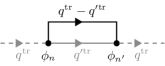
Figure 6: In order to describe the presence of offset charges, a virtual branch (solid black line) representing the effect of the displacement currents is added in parallel to each tree branch of the original circuit (solid gray line). As a consequence, the charge $q^{\text{tr}}$ entering the tree branch splits into the charge $q^{\prime\text{tr}}$ on the tree element and the charge $q^{\text{tr}}-q^{\prime\text{tr}}$ on the virtual branch. The current flowing away from node $n$ and $n^{\prime}$ into the subgraph (gray) is given by $\pm(q^{\prime\text{tr}}-q^{\text{tr}})$. Ensuring the Kirchhoff laws therefore requires adding the terms $-(\phi_{n}-\phi_{n^{\prime}})(\dot{q}^{\prime\text{tr}}-\dot{q}^{\text{tr}})=-\phi^{\text{tr}}(\dot{q}^{\prime\text{tr}}-\dot{q}^{\text{tr}})$ with the tree branch flux $\phi^{\text{tr}}=\phi_{n}-\phi_{n^{\prime}}$ to the Lagrangian.

Let us now use these results to prove the rules for the inclusion of offset charges described in Sec. II.2. As we have discussed there, offset charges must be modeled through the inclusion of additional lumped elements in the circuit. These elements are naturally described in terms of node fluxes since they modify the current balance. Therefore, in order to describe the presence of offset charges $\bm{q}^{\text{ex}}$ on the nodes of the circuit, we add to each of the tree branches with charges $\bm{q}^{\text{tr}}$ another virtual parallel branch which will represent the action of the displacement currents and will be described in terms of node fluxes. As a consequence, only a fraction $\bm{q}^{\prime\text{tr}}$ of the total charge $\bm{q}^{\text{tr}}$ entering the branches will remain on the original tree element, while the charge $\bm{q}^{\text{tr}}-\bm{q}^{\prime\text{tr}}$ will reside on the virtual branch. Since the equations of motion with respect to $\bm{\phi}$ yield the currents flowing away from the respective nodes, offset charges $\bm{q}^{\text{ex}}$ on the nodes of the circuit correspond to a term $\dot{\bm{\phi}}\cdot\bm{q}^{\text{ex}}$ in the Lagrangian. In order to ensure the Kirchhoff laws, we also have to add the terms $-\bm{\phi}^{\text{tr}}\cdot(\dot{\bm{q}}^{\prime\text{tr}}-\dot{\bm{q}}^{\text{tr}}$), c.f. Fig. 6.

We have already discussed in in Sec. III.1 that the node-edge incidence matrix $A$ relates the branch fluxes and the node fluxes as $\bm{\phi}^{\text{br}}=A^{T}\bm{\phi}$. A decomposition of $\bm{q}^{\text{br}}=(\bm{q}^{\text{ch}},\bm{q}^{\text{tr}})$ into the vector of chord charges $\bm{q}^{\text{ch}}$ and tree charges $\bm{q}^{\text{br}}$ gives rise to a corresponding decomposition of $A=(A_{\text{ch}},A_{\text{tr}})$ with $A_{\text{tr}}$ a square matrix. Since there are no loops in a tree, we have the result $A_{\text{tr}}\bm{v}\neq 0$ for every vector $\bm{v}\in\mathbb{R}^{b}$, implying that $A_{\text{tr}}$ has full rank and the inverse $A_{\text{tr}}^{-1}$ is well-defined *[][; Theorem2.2.]chen. With the help of the matrix $A$, we can write the expression added to the Lagrangian in the form $\dot{\bm{\phi}}\cdot\bm{q}^{\text{ex}}-\bm{\phi}\cdot A_{\text{tr}}(\dot{\bm{q}}^{\prime\text{tr}}-\dot{\bm{q}}^{\text{tr}})$. Since $A_{\text{tr}}$ is invertible, the equations of motion with respect to $\bm{\phi}$ yield the constraint $\dot{\bm{q}}^{\prime\text{tr}}=\dot{\bm{q}}^{\text{tr}}-A_{\text{tr}}^{-1}\dot{\bm{q}}^{\text{ex}}$. As a result, we can simply ignore the virtual branches just introduced and continue working with the original circuit graph, provided we simply replace each expression in the Lagrangian involving the tree charge $\bm{q}^{\text{tr}}$ by $\bm{q}^{\prime\text{tr}}$. It can be shown that for all nodes $j$ that are connected to ground through branch $i$, the entries of $(A_{\text{tr}}^{-1})_{ij}$ are given by $\pm 1$ depending on whether branch $i$ points towards or away from ground, while they are zero for all other nodes chen . Using this, we reproduce the rules given previously. We show in the App. C that proceeding similarly for a circuit with external fluxes that is described in terms of node fluxes recovers the rules given in Ref. devoret:96, .

For completeness, we note that no such simple rule emerges if one intends a mixed description of the circuit. In that case, one does not get around representing external fluxes and offset charges explicitly through virtual additional circuit elements. For an external flux $\Phi^{\text{ex}}_{l}$ in some loop $l$ with loop charge $Q_{l}$ which is part of the subgraph or an offset charge $q^{\text{ex}}_{n}$ at some node $n$ which is either part of the subgraph complement or a boundary node, those virtual elements are easy to handle. In that case, they simply add the terms $\dot{Q}_{l}\Phi_{l}^{\text{ex}}$, $\dot{\phi}_{n}q^{\text{ex}}_{n}$ to the Lagrangian without requiring additional terms to guarantee the Kirchhoff laws. For external fluxes in loops that lie completely within the subgraph complement or offset charges at the nodes of the subgraph (without the boundary nodes), however, the additional terms guaranteeing the Kirchoff laws have to be added by hand.

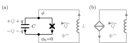
Figure 7: In (a), we show the idealized exact fluxonium circuit and in (b), we show the approximate fluxonium representation obtained after exploiting the passive duality transformation explained in Sec. VI.1. The gray part of the circuit denotes the subgraph described by loop charges.

As an example, we consider the fluxonium circuit depicted in Fig. 7. We describe the inductive shunt in terms of loop charges and the rest of the circuit in terms of node fluxes. Using the rules given above, we obtain the Lagrangian

$$\mathcal{L}=\frac{C}{2}\dot{\phi}^{2}+E_{J}\cos\biggl{(}\frac{2\pi\phi}{\Phi_{Q}}\biggr{)}+\frac{L}{2}\dot{Q}^{2}-Q\dot{\phi}+\dot{Q}\Phi^{\text{ex}}$$ (27)

with $E_{J}=\Phi_{Q}I_{c}/2\pi$. Here, the first two terms are due to the Josephson junction and its associated capacitance, which are described in terms of node fluxes, while the term $L\dot{Q}^{2}/2$ is due to the inductive shunt within the subgraph which is described in terms of loop charges. The voltage drop $\dot{\phi}$ in the direction of the loop charge $Q$ gives the term $-Q\dot{\phi}$ guaranteeing the Kirchhoff voltage and current law. The external flux $\Phi^{\text{ex}}$ within the boundary loop adds the term $\dot{Q}\Phi^{\text{ex}}$. Since we describe the inductive shunt in terms of the polarization charge $Q$, we have to take $\phi$ to be $\Phi_{Q}$-periodic since only integer number of Cooper-pairs can flow from the ground to the node with flux $\phi$ in absence of the inductive shunt. Performing the Legendre transformation, we obtain the Hamiltonian apenko:89 ; zaikin:90

$$H_{\text{flux}}=\frac{(q+Q)^{2}}{2C}-E_{J}\cos\biggl{(}\frac{2\pi\phi}{\Phi_{Q}}\biggr{)}+\frac{(\Phi-\Phi^{\text{ex}})^{2}}{2L},$$ (28)

where $q=\partial\mathcal{L}/\partial\dot{\phi}$ and the total flux $\Phi=\partial\mathcal{L}/\partial\dot{Q}$ are canonically conjugate to $\phi$ and $Q$. The Hamiltonian acts on wavefunction of the form $\psi(\phi,\Phi)$, where $\phi$ is periodic (with period $\Phi_{Q}$).

The capacitive term of the Hamiltonian (28) reveals that the physical charge $\tilde{q}=q+Q$ on the capacitor plate is the sum of the charge $q\in 2e\mathbb{Z}$ (flowing through the Josephson junction) and $Q$ (flowing through the inductor). As the charges do not enter individually, the operator $e^{i(\phi-\Phi)/\Phi_{Q}}$ commutes with the Hamiltonian. As a result, we obtain that the fluxes are equal with $\tilde{\phi}=\Phi=\phi$, where the last equality holds modulo $\Phi_{Q}$.Note3 We introduce the new wavefunction

$$\tilde{\psi}(\tilde{\phi})=\psi(\tilde{\phi},\tilde{\phi})$$ (29)

with $-i\hbar\partial_{\tilde{\phi}}\tilde{\psi}(\tilde{\phi})=(q+Q)\psi(\phi,\Phi)$ such that the charge $\tilde{q}$ on the capacitor plate is the conjugate variable to $\tilde{\phi}$. With that, we have decompactified the phase $\phi$ (defined on the interval $[0,\Phi_{Q}]$) to $\tilde{\phi}$ (defined on the complete real line). This gives the conventional form of the fluxonium Hamiltonian (acting on the wavefunction $\tilde{\psi}$)

$$\tilde{H}_{\text{flux}}=\frac{\tilde{q}^{2}}{2C}-E_{J}\cos\biggl{(}\frac{2\pi\tilde{\phi}}{\Phi_{Q}}\biggr{)}+\frac{1}{2L}(\tilde{\phi}-\Phi^{\text{ex}})^{2},$$ (30)

with $\tilde{q}$ the conjugate variable to $\tilde{\phi}$. Alternatively, in the path integral formulation, one can start with (28) and integrate out the harmonic mode $Q$ in order to arrive at (30) apenko:89 ; zaikin:90 .

It has previously been shown that in the limit $L\rightarrow\infty$, selection rules emerge from the Hamiltonian (30) which limit the dynamics of the decompactified variable $\tilde{\phi}$ to the dynamics of a compact variable $\phi$ corresponding to the system without a shunt koch:09 . The origin of the selection rules is made transparent by the Hamiltonian (28) which shows that polarization charge $Q$ becomes conserved in the limit $L\rightarrow\infty$. The explicit separation of the transport of $q$ over the Josephson junction and the flow of polarization charge $Q$ through the shunt in the Hamiltonian (28) clearly brings out the different time scales associated with the two processes. This fact makes it very useful for the derivation of an effective fluxonium Hamiltonian as we will discuss in Sec. VI.1.

As another example of the mixed formulation, we discuss in the App. E the derivation of a Hamiltonian for the experimental setup of Ref. vogt:15, .

VI Applications

As we have discussed in the previous sections, Josephson junctions cannot be handled directly using loop charges. On the other hand, it is well-known that Josephson junctions are approximately self-dual mooij:06 and can behave as nonlinear capacitors at low energies. As we now want to show, this yields an approximate way of incorporating Josephson junctions in the loop charge description.

In particular, we discuss the example of a single Josephson junction: the effective nonlinear capacitor is given by the $2e$-periodic ground-state energy $\varepsilon_{0}(Q)$, where $Q$ is the polarization charge. An instructive way to understand the $2e$ periodicity is provided by writing the total charge on capacitor plate as the sum $q+Q$ of the integer charge $n=q/2e$ and the continuous polarization charge $Q$, cf. Eq. (30).schon:90 While the former corresponds to (excess) Cooper-pairs on the island, the latter models the polarization charge, i.e., continuous displacements of negative and positive charges on the island against each other due to polarizing electric fields. The unusual aspect of the Josephson junction is the fact that it allows exchange of individual Cooper-pairs through tunneling, whereas the polarization charge remains fixed due to the insulating layer of the Josephson junction. As a result, a Josephson junction is only able to screen the charges in units of $2e$ yielding the periodic ground state energy $\varepsilon_{0}(Q)$.

The separation of the charge $q+Q$ remains useful when shunting the Josephson junction by a large (complex) impedance $Z_{\omega}$ that allows the exchange of the polarization charge between the capacitor plates. As long as the impedance is large, there will be an adiabatic separation of the fast flow of integer charges $n$ through the Josephson junction and the polarization charge flow through the shunt. We will make this idea in two examples more explicit.

VI.1 Fluxonium

We now want to apply this idea in the description of the fluxonium circuit of Fig. 7.manucharyan:09 In the limit of large inductance $L$, the shunt impedance $Z_{\omega}=-i\omega L$ becomes large and we can perform the adiabatic decoupling of the polarization charge $Q$ and the phase $\phi$ in the fluxonium Hamiltonian (28). To that end, we introduce the (instantaneous) eigenstates $u_{Q,s}(\phi)$ of the Cooper-pair box Hamiltonian

$$H_{\text{cpb}}=\frac{1}{2C}\biggl{(}-i\hbar\frac{\partial}{\partial\phi}+Q\biggr{)}^{2}-E_{J}\cos\biggl{(}\frac{2\pi\phi}{\Phi_{Q}}\biggr{)},$$ (31)

such that $H_{\text{cpb}}\,u_{Q,s}(\phi)=\varepsilon_{s}(Q)\,u_{Q,s}(\phi)$ holds, where $\varepsilon_{s}(Q)$ is the $2e$-periodic instantaneous eigenenergy to the (constant) polarization charge $Q$. In the adiabatic approximation, we make the ansatz $\psi(\phi,Q)=u_{Q,s}(\phi)\chi_{s}(Q)$ for the total wavefunction of $H_{\text{flux}}$ in Eq. (28). Inserting this ansatz and neglecting derivatives of $u_{Q,s}$ with respect to $Q$, we arrive at the lowest-order adiabatic approximation bohm ; zorin:06 ; koch:09

$$H_{s}=\frac{1}{2L}\biggl{(}i\hbar\frac{\partial}{\partial Q}-\Phi^{\text{ex}}\biggr{)}^{2}+\varepsilon_{s}(Q)$$ (32)

for the Hamiltonian of the wavefunction $\chi_{s}(Q)$ which is $2e$ periodic. The Hamiltonian (32) is the (passive) dual description a Josephson junction shunted by a large impedance as alluded to in the introduction and depicted in Fig. 7.

We want to comment on the connection of the wavefunctions $\chi_{s,n}(Q)$ for the $n$-th eigenstate obtained in this manner to the wavefunction $\tilde{\psi}(\tilde{\phi})$ of the (conventional) fluxonium Hamiltonian $\tilde{H}_{\text{flux}}$ of Eq. (30). Using the relation (29) as well as the adiabatic ansatz, we obtain

$$\tilde{\psi}_{s,n}(\tilde{\phi})=\int_{0}^{2e}\!\frac{dQ}{2\pi\hbar}u_{Q,s}(\tilde{\phi})\chi_{s,n}(Q)e^{iQ\tilde{\phi}/\hbar},$$ (33)

as an approximate expression of the exact eigenstates.

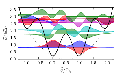
Figure 8: Exact ($\tilde{\phi}<\Phi_{Q}/2$) and approximate ($\tilde{\phi}>\Phi_{Q}/2$) fluxonium wave functions for $\Phi^{\text{ex}}=\Phi_{Q}/2$. The exact wave functions are computed by exact diagonalization of the full Hamiltonian (30) and the approximate wave functions are obtained by computing eigenstates $\chi_{s,n}(Q)$ of the adiabatic Hamiltonian (32) and using formula (33). The states live in a potential (solid black line) composed of a harmonic contribution (dashed black line) due to the inducance with an inductive energy $E_{L}=(\Phi_{Q}/2\pi)^{2}/L$ and the superposed cosine potential due to the Josephson junction with the Josephson energy $E_{J}$. The parameters $E_{J}/4E_{C}=0.9$ and $E_{L}/4E_{C}=0.052$ (with the capacitive energy $E_{C}=e^{2}/2C$) correspond to the qubit discussed in Ref. manucharyan:09, . The wave functions of both Hamiltonians can be chosen real due to the symmetry under $(\phi,\Phi)\mapsto(-\phi,\Phi_{Q}-\Phi)$ and are centered vertically at their corresponding energy eigenvalue.

To highlight the accuracy of the approximate expression (33), we have numerically calculated the eigenstates $\tilde{\psi}_{m}(\tilde{\phi})$ of the Hamiltonian (30), as explained in App. F, and the eigenstates $\chi_{s,n}(Q)$ and $u_{Q,s}(\phi)$ of the Hamiltonians (32) and (31). In Fig. 8, we show the comparison of the exact eigenstates to the approximate eigenstates (33) for $\Phi^{\text{ex}}=\Phi_{Q}/2$. Note that the wave functions can be chosen real due to the symmetry under $\tilde{\phi}\mapsto\Phi_{Q}-\tilde{\phi}$ (or, $(\phi,\Phi)\mapsto(-\phi,\Phi_{Q}-\Phi)$, respectively) and are centered vertically at their corresponding energy value. Especially for the low-lying states, one sees good agreement between the exact eigenstates and the approximate states (33). In particular, for the exact lowest energy states $\tilde{\psi}_{g}$, $\tilde{\psi}_{e}$ of the fluxonium Hamiltonian (30), we find the correspondence

$$\bigl{(}\tilde{\psi}_{g},\tilde{\psi}_{e}\bigr{)}\mapsto(\tilde{\psi}_{0,0},\tilde{\psi}_{0,1}),$$ (34)

i.e., the states $\tilde{\psi}_{g}$, $\tilde{\psi}_{e}$ are all associated with the lowest $s=0$ band of the Cooper-pair box. As we show in Fig. 9, this property persists for the entire range of external flux $\Phi^{\text{ex}}$. In particular around the experimentally relevant flux bias of half a flux quantum, $\Phi^{\text{ex}}=\Phi_{Q}/2$, we find overlaps $|\langle\tilde{\psi}_{g}|\tilde{\psi}_{0,0}\rangle|$, $|\langle\tilde{\psi}_{e}|\tilde{\psi}_{0,1}\rangle|$ well above $0.95$. We thus arrive at the conclusion that the fluxonium can effectively be understood as a phase-slip junction with a constitutive relation $V=f_{V}(Q)=\epsilon_{0}^{\prime}(Q)$. Instead of using the original fluxonium circuit from Fig. 7(a), we may therefore obtain an accurate description in terms of the simpler circuit depicted in Fig. 7(b), which follows from the first circuit by replacing the Josephson junction and its associated capacitance by a phase slip junction.

The circuit from Fig. 7(b) yields a simplified fluxonium description which may, e.g., be convenient in order to understand the effects of environmental noise. As an example, we consider the case of a noisy inductor which we model by an additional resistor $R$ in series with the inductance $L$. The flux $\phi$ over the resistor couples linearly to the current $\dot{Q}$ and we can therefore apply the results of Sec. IV. Using standard results for qubits makhlin:01 ; nazarov_noise_schoelkopf , one arrives at a relaxation rate

$$\Gamma_{1}=\frac{|\langle\chi_{0,0}|\partial_{Q}|\chi_{0,1}\rangle|^{2}}{L^{2}}\,S_{\phi}(E_{01}/\hbar),$$ (35)

where $E_{01}>0$ denotes the energy difference between the states $\chi_{0,1}$ and $\chi_{0,0}$ and $S_{\phi}(\omega)=\int\!dt\,e^{i\omega t}\langle\phi(t)\phi(0)\rangle=2\hbar R(n_{\omega}+1)/\omega$ is the spectral density of flux fluctuations over the resistor. In units of the RL-time $\tau_{\text{RL}}=L/R$, the result reads $\Gamma_{1}\tau_{\text{RL}}=(n_{B}+1)\Phi_{01}^{2}/LE_{01}$ with $n_{B}$ the photon number at frequency $\omega=E_{01}/\hbar$. As a result, the decay $\Gamma_{1}$ is proportional to the ratio of the magnitude of energy fluctuations $\Phi^{2}_{01}/L$ due to the (quantum) fluctuations of $\Phi$ to the energy difference of the transition.

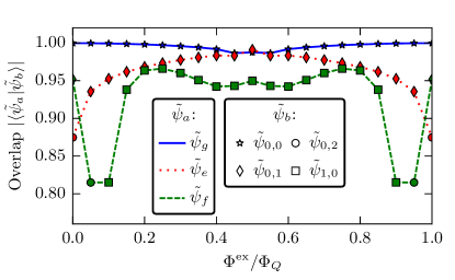
Figure 9: Approximate fluxonium eigenstates $\tilde{\psi}_{s,n}$ which have the maximum overlap with either of the three lowest energy states $\tilde{\psi}_{g}$, $\tilde{\psi}_{e}$, $\tilde{\psi}_{f}$ of the exact fluxonium Hamiltonian (30). The approximate eigenstates are calculated via Eq. (33), using the eigenstates of the Hamiltonian (32) which arises from projection on band $s$ of the Cooper-pair box Hamiltonian (31).

VI.2 $0$-$\pi$ qubit

As another example, we consider the $0$-$\pi$ qubit, which is based on a special type of Josephson inductance that is $\Phi_{Q}/2$-periodic in the phase $\phi$. This has to be contrasted with the $\Phi_{Q}$-periodicity found in conventional Josephson junctions. There exist two different proposals for its realizations. The first proposal, the superconducting current mirror, is based on an energetic suppression of single Cooper-pair tunneling kitaev:06a , whereas the second proposal, the Josephson rhombus, is based on destructive interference of single Cooper-pair tunneling guaranteed through symmetry doucot:02 ; doucot:12 . Independent of the specific way the $\Phi_{Q}/2$-periodic junction is realized, its effective Hamiltonian can be written as

$$H=4E_{C}(q+Q)^{2}-E_{J2}\cos(4\pi\phi/\Phi_{Q}),$$ (36)

where $q=-i\hbar\partial/\partial\phi$ is conjugate to $\phi$, $E_{J2}$ gives the strength of the $\Phi_{Q}/2$-periodic junction and we have included a charging energy with polarization charge $Q$.

There exist two possible choices of qubit states. When the junction strength is much larger than the charging energy, $E_{J2}/E_{C}\gg 1$, the states can be approximated as states localized at the potential minima $\phi=0$ or $\phi=\Phi_{Q}/2$ of the junction term. On the other hand, it is clear that the correct eigenstates of the Hamiltonian (36) are characterized by Cooper-pair parity as a good quantum number, since the $E_{J2}$ term only connects charge states differing by $4e$. Indeed, tunneling between the minima of the junction leads to a hybridization of the states localized at $\phi=0$ or $\phi=\Phi_{Q}/2$ into odd and even superpositions $\psi_{o}$, $\psi_{e}$ which are in direct correspondence to states characterized by odd or even Cooper-pair parity bell:14 . This is illustrated in Fig. 10(a) for $E_{J2}=20E_{C}$ and $Q=0$. Going over to a Bloch band description with the choice of a $\Phi_{Q}/2$-periodic unit cell allows mapping the Hamiltonian (36) to the Hamiltonian of the conventional Cooper-pair box. One can then use the semiclassical results for the $2e$-periodic charge dispersion of the lowest band of the conventional Cooper-pair box koch:07 . After the appropriate scaling, it maps to the $4e$-periodic charge dispersion $\varepsilon_{0}=-A\cos(\pi Q/2e)+\text{const.}$ with bandwidth $2A$, where $A$ is given by

$$A=2^{6}\sqrt{\frac{2}{\pi}}\Biggl{(}\frac{E_{J2}}{8E_{C}}\Biggr{)}^{\tfrac{3}{4}}E_{C}e^{-\sqrt{2E_{J2}/E_{C}}}.$$ (37)

For the lowest band, the exact charge dispersion (solid line) and its asymptotic expression (37) (dashed line) is illustrated in Fig. 10(b) for the same parameters $E_{J2}=20E_{C}$ as in (a). Going back to a $\Phi_{Q}$-periodic unit cell corresponds to folding the Bloch-bands for $Q>2e$ back to the origin. The resulting band structure is displayed in Fig. 10($c$). The states from the lowest two bands are the qubit states $\psi_{e}$, $\psi_{o}$ corresponding to even or odd Cooper-pair parity. In the regime $E_{J2}\gg E_{C}$, the gap $E_{eo}$ between the two states roughly scales as $E_{eo}=2A\propto e^{-\sqrt{2E_{J2}/E_{C}}}$.

The question of which choice of states adequately describes the qubit depends on the size of perturbations that yield transitions between states of different Cooper-pair parity. Such a perturbation is, e.g., a finite amplitude $E_{J1}$ for tunneling of conventional Cooper-pairs. An amplitude $E_{J1}$ that is much larger than the gap $E_{eo}$ will lead to a rapid dephasing of the superpositions in the states $\psi_{e}$, $\psi_{o}$ and effectively project back to the states localized at the potential minima.

For the following, we are interested in the regime where $E_{J1}$ is smaller than $E_{eo}$. Note that this is, e.g., the regime of the experiments discussed in Ref. bell:14, . In this case, the Cooper-pair parity and the offset charge $Q$ in the interval $(0,2e)$ remain good quantum numbers and the level structure can be represented as indicated in Fig. 10(c). Note that the crossing of the two level curves is protected as long as Cooper-pair parity is conserved.

It is intriguing to note that there is an obvious duality between the charge dispersion of the $0$-$\pi$ qubit shown in Fig. 10(c) and the flux dispersion of a junction connecting two Majorana bound states with energy (fractional Josephson effect) kitaev:01

$$H=\pm\cos(\pi\phi/\Phi_{Q}),$$ (38)

where the choice of the plus or minus sign is related to the occupation parity of the nonlocal fermion hosted by the Majorana bound states. Dual to the treatment of the $0$-$\pi$ qubit, one can describe the $2\Phi_{Q}$-periodic Majorana junction in terms of a folded zone-scheme in a $\Phi_{Q}$-periodic unit cell, leading to a similar picture as in Fig. 10(c) but with $Q/2e$ replaced by $\phi/\Phi_{Q}$. Now the two bands differ in superconducting flux quantum parity and the crossing at $\Phi_{Q}/2$ is protected as long as flux quantum parity is preserved. This corresponds to an absence of conventional Josephson junctions in a loop with the Majorana junction through which conventional $\Phi_{Q}$ phase-slips may occur heck:11 .

Embedding the $0$-$\pi$ circuit in a large-impedance environment as discussed in Sec. VI leads to a low-energy description by states living in the charge-dispersion bands from Fig. 10(c). With this starting point, one may consider more complex circuits. We thus arrive at there intriguing conclusion that the $0$-$\pi$ qubit may allow us to explore the plethora of proposals existing for Majorana qubits beenakker:13 ; stanescu:13 from a dual perspective.

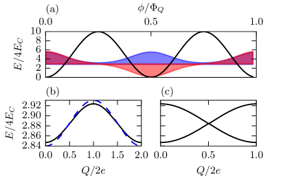
Figure 10: In (a), we show the two lowest-energy wave functions of the $0$-$\pi$ Hamiltonian (36) for $E_{J2}=20E_{C}$ and $Q=0$. The wave functions can be chosen real and are centered vertically at their corresponding energy. One observes the even or odd character of the eigenstates under translations by $\Phi_{Q}/2$ which reflects the Cooper-pair parity of the states. In (b), we illustrate the Bloch bands originating from the choice of a $\Phi_{Q}/2$-periodic unit cell, resulting in Bloch-band periodicity of $4e$. The asympotic estimate (37) valid for $E_{J2}\gg E_{C}$ is shown as a blue dashed line. In (c), we illustrate the folded zone scheme corresponding to the choice of a $\Phi_{Q}$-periodic unit cell which arises from (b) by folding the part of the Bloch bands for $Q>2e$ back. The two resulting bands differ in Cooper-pair parity. The band crossings at $Q=e$ are protected as long as Cooper-pair parity is conserved.

VII Conclusions

In this paper, we have discussed a charge-based approach to circuit quantization using loop charges which are the time-integrated currents circulating in the loops of a planar circuit. We have shown that the appropriate circuit Lagrangian can be read off the electrical network using a set of simple rules. In this approach, we obtain a local Hamiltonian description in terms of charges in a planar circuits of arbitrary topology. We have discussed how to handle dissipative elements by going over from closed systems to open systems.

We have shown explicitly that a passive duality transformation relates the charge-based circuit description in terms of loop charges to the flux-based description in terms of node fluxes which is conventionally employed for the quantization of superconducting circuits. While the flux-based formulation is convenient for the description of charge currents, the charge-based formulation yields a simple description whenever the dynamics is characterized by flux currents. In particular, we have argued that passive duality transformations are useful for Josephson junctions in large-impedance environments, which behave as nonlinear capacitors supporting a quantized flux flow at low energies.

We have shown that the loop charge formulation can be used more generally for the description of arbitrary circuits involving phase-slip junctions which are nonlinear capacitors electromagnetically dual to Josephson junctions. We have explained that electromagnetic duality can be used as an active transformation yielding new circuits whose charge dynamics is identical to the flux dynamics of the original circuit. We have shown how the loop charge formalism allows the straightforward construction of such active duality transformations. In particular, Josephson junctions have to be replaced by phase-slip junctions. The duality between the node fluxes and the loop charges guarantees that the loop charges are useful for the description of latter circuits in the same way that node fluxes are useful for Josephson junction circuits.

We have introduced a mixed circuit description in terms of loop charges and node fluxes. We have shown that the mixed formulation gives additional insights into the decompactification of the flux $\phi$ over a Josephson junction that is shunted by an inductor.

We have explicitly illustrated how passive duality transformations yield simplified circuit descriptions for Josephson junctions shunted by large impedances using the fluxonium qubit and the $0$-$\pi$ qubit as an example. We have shown that regarding the fluxonium as a nonlinear capacitor yields an approximate though accurate description of the qubit states for relevant qubit parameters. We have illustrated how this may be used, e.g., for a simplified description of relaxation caused by environmental noise. As another example, we have considered the $0$-$\pi$ qubit. We have shown that in the absence of conventional Cooper-pair tunneling, the junction dynamics becomes electromagnetically dual to the dynamics of a Majorana Josephson junction.

From this work, several interesting routes arise that could be explored in the future. It will be highly interesting to use the loop charge formalism for quantitative analysis of recent experiments involving phase-slip junctions. It will also be interesting to exploit the duality of the $0$-$\pi$ qubit to a Majorana junction and explore existing proposals for Majorana physics from a dual perspective.

Appendix A Mathematical preliminaries

For the convenience of the reader, we here want to rederive the standard result of circuit analysis chen ; thulasiraman that in a planar circuit, loop charges $\bm{Q}$ determine all the branch currents $\dot{\bm{q}}^{\text{br}}$ in such a way that the Kirchhoff current law is fulfilled. Along the way, we will recall a few standard mathematical results about graphs that will be used in the remainder of the appendix. More information can be found in the literature chen ; thulasiraman .

We first need to show that there is an independent current for each of the $m$ chords of the spanning tree. To see that the Kirchhoff current law implies precisely $m$ independent currents, we make use of the basis node-edge incidence matrix $A$, which is a $\mathbb{R}^{(n-1)\times b}$ matrix for the $n-1$ nodes without the ground node and the $b$ branches. Its entries $A_{ij}\in\{1,-1\}$ indicate whether branch $j$ enters ($-1$) or leaves $(+1)$ node $i$. Given a vector $\bm{q}^{\text{br}}$ of branch charges, the Kirchhoff current law can be expressed as $A\dot{\bm{q}}^{\text{br}}=0$. A decomposition of $\bm{q}^{\text{br}}=(\bm{q}^{\text{ch}},\bm{q}^{\text{tr}})$ into the vector of chord charges $\bm{q}^{\text{ch}}$ and tree charges $\bm{q}^{\text{br}}$ gives rise to a corresponding decomposition of $A=(A_{\text{ch}},A_{\text{tr}})$. Since there are no loops in a tree, we have the result $A_{\text{tr}}\bm{v}\neq 0$ for every vector $\bm{v}\in\mathbb{R}^{b}$, implying that $A_{\text{tr}}$ has full rank and the inverse of $A_{\text{tr}}^{-1}$ is well-defined *[][; Theorem2.2.]chen. One can also show the result $\left|\det A_{\text{tr}}\right|=1$. Using that $A_{\text{tr}}^{-1}$ is invertible, we obtain the relation $\dot{\bm{q}}^{\text{tr}}=-A_{\text{tr}}^{-1}A_{\text{ch}}\dot{\bm{q}}^{\text{ch}}$, showing that the $m$ chord charges $\bm{q}^{\text{ch}}$ fully specify all currents in the circuit.

Our intuitive notion that the loop currents give the correct number of independent currents in a planar graph is confirmed by Euler’s theorem for connected planar graphs which is the relation $n-b+f=2$, where $f$ is the number of faces of a graph. Using $b=m+n-1$, we obtain $f=m+1$, where the $+1$ arises since $f$ also counts the exterior of the planar graph as a face. This shows that the loop charges in the faces of the graph indeed give the correct number of independent currents for a planar circuit. More generally, one can show thulasiraman that this is no longer case for a nonplanar graph.

It remains to relate the chord charges $\bm{q}^{\text{ch}}$ more explicitly to the loop charges $\bm{Q}$. To characterize the change of variables from $\bm{q}^{\text{ch}}$ to $\bm{Q}$, we note that we may characterize the loops of a circuit in terms of the fundamental circuit matrix $B\in\mathbb{R}^{m\times b}$, where each entry $B_{ij}\in\{1,-1\}$ indicates that the branch $j$ is oriented in the same direction ($1$) or opposite ($-1$) to the arbitrarily chosen orientation of the loop $i$ formed by the $i$-th chord and the branches of the spanning tree. The matrix $B$ obeys the important relation $AB^{T}=0$ which expresses the fact that for each node that is part of some loop, branches having the same incidence orientation with respect to the node will necessarily have opposite orientations with respect to the loop. From the relation $AB^{T}=0$ and the decomposition $A=(A_{\text{ch}},A_{\text{tr}})$, we obtain the expression $B^{\prime}=(1,-A_{\text{ch}}^{T}(A_{\text{tr}}^{-1})^{T})$ for the fundamental circuit matrix corresponding to the loop basis induced by the chords. For the loop basis corresponding to the loop charges we have the more general form $B=(B_{\text{ch}},B_{\text{tr}})$ where $B_{\text{ch}}$ is invertible since it is related to the identity matrix via a basis transformation in loop space. This finally gives the relation $\bm{q}^{\text{ch}}=B_{\text{ch}}^{T}\bm{Q}$.

By definition of the matrices $A$ and $B$, we obtain the results $\dot{\bm{q}}^{\text{br}}=B^{T}\dot{\bm{Q}}$ and $\dot{\bm{\phi}}^{\text{br}}=A^{T}\dot{\bm{\phi}}$. Making use of the relation $AB^{T}=0$ shows that the branch fluxes and branch charges defined in this way automatically fulfill the Kirchhoff voltage law $B\dot{\bm{\phi}}^{\text{br}}=0$ and the Kirchhoff current law $A\dot{\bm{q}}^{\text{br}}=0$.

Appendix B Duality in the path integral

Our starting point is expression (13),

$$e^{(i/\hbar)\int^{t}\!dt^{\prime}\,\mathcal{L}(\bm{\phi}^{\text{br}})}=\int\mathcal{D}[\bm{q}^{\text{br}}(t)]e^{(i/\hbar)\int^{t}\!dt^{\prime}[\tilde{\mathcal{L}}(\bm{q}^{\text{br}})-\bm{q}^{\text{br}}\cdot\dot{\bm{\phi}}^{\text{br}}]}.$$ (39)

For the decomposition $\bm{q}^{\text{br}}=(\bm{q}^{\text{ch}},\bm{q}^{\text{tr}})$ of the branch charges, we have found in App. A the relation $\dot{\bm{q}}^{\text{tr}}=-A_{\text{tr}}^{-1}A_{\text{ch}}\dot{\bm{q}}^{\text{ch}}$, which shows that the chord charges $\bm{q}^{\text{ch}}$ determine the tree charges $\bm{q}^{\text{ch}}$ up to constant offset charges $\bm{\lambda}$. We can make this explicit by introducing the factor

$$1=\int\mathcal{D}[\bm{\lambda}(t)]\,\delta[(\bm{q}^{\text{tr}}+A_{\text{tr}}^{-1}A_{\text{ch}}\bm{q}^{\text{ch}}-\bm{\lambda})(t)]$$ (40)

into the integral (39). Using the relation $\bm{\phi}^{\text{br}}=A^{T}\bm{\phi}$ for the vector of node fluxes $\bm{\theta}$ and performing the integration over the tree charges $\bm{q}^{\text{tr}}$ yields

$$e^{(i/\hbar)\int^{t}\!dt^{\prime}\,\mathcal{L}(\bm{\phi}^{\text{br}})}=\int\mathcal{D}[\bm{\lambda}(t)]\int\mathcal{D}[\bm{q}^{\text{ch}}(t)]\\ \times e^{(i/\hbar)\int^{t}\!dt^{\prime}[\tilde{\mathcal{L}}(\bm{q}^{\text{ch}},-A_{\text{tr}}^{-1}A_{\text{ch}}\bm{q}^{\text{ch}}+\bm{\lambda})-\bm{\lambda}A_{\text{tr}}^{T}\dot{\bm{\phi}}]}.$$ (41)

Performing a partial integration on the term $-i\bm{\lambda}A_{tr}^{T}\dot{\bm{\phi}}/\hbar$ in the exponent, inserting the resulting expression in Eq. (12) and performing the integration over the node fluxes $\bm{\phi}$, we obtain a constraint at each point in time in terms of the delta function $\delta[A_{\text{tr}}\dot{\bm{\lambda}}(t)]$. Since $A_{\text{tr}}$ has full rank and obeys $|\det A_{\text{tr}}|=1$, this is equivalent to demanding $\dot{\bm{\lambda}}=0$ for all times. We resolve this constraint by demanding that offset charges are constant, $\bm{\lambda}(t)\equiv\bm{\lambda}$. In fact the value of $\bm{\lambda}=0$ is fixed by the boundary condition that all the elements are uncharged for $t\to-\infty$. We thus obtain the representation

$$e^{-iHt/\hbar}\rightarrow\int\mathcal{D}[\bm{q}^{\text{ch}}(t)]\\ \times e^{(i/\hbar)\int^{t}\!dt^{\prime}\,\tilde{\mathcal{L}}[\bm{q}^{\text{ch}},-A_{\text{tr}}^{-1}A_{\text{ch}}\bm{q}^{\text{ch}}]},$$ (42)

for the time-evolution operator. In a planar circuit, we may finally exploit the relation $\bm{q}^{\text{ch}}=B_{\text{ch}}^{T}\bm{Q}$ and replace the integration over $\bm{q}^{\text{ch}}$ by an integration over the loop charges $\bm{Q}$. We then recover expression (15) from the main text.

Appendix C Equivalence of terms manifestly guaranteeing the Kirchhoff current law or the voltage law in the mixed formulation

We want to prove the equality (up to a total time-derivative) of the term $-\sum_{i}\phi^{\partial}_{i}\sum_{j}\dot{q}_{ij}$ manifestly guaranteeing the Kirchhoff current law and the term $-\sum_{i}Q^{\partial}_{i}\sum_{j}\dot{\phi}_{ij}$ manifestly guaranteeing the Kirchhoff voltage law.

Let $P\in\mathbb{R}^{b\times b}$ be the matrix projecting on the branches (the subgraph) that shall be described in terms of loop charges. We note that we have the identity

$$-\sum_{i}\phi^{\partial}_{i}\sum_{j}\dot{q}_{ij}=-\bm{\phi}APB^{T}\dot{\bm{Q}},$$ (43)

where $B$ is the fundamental circuit matrix introduced in App. A corresponding to the loop charges $\bm{Q}$. This identity can be understood by noting that $PB^{T}\dot{\bm{Q}}$ is the projection of the vector of branch currents onto the branches of the subgraph. The expression $(APB^{T}\dot{\bm{Q}})_{i}$ gives the current balance for each node $i$ of the subgraph. According to the definition of the basis node-edge incidence matrix $A$, positive currents flowing away from node $i$ come with a plus sign, while positive currents flowing into node $i$ come with a minus sign. In line with the definition of the $\dot{q}_{ij}$, one thus obtains in both cases the current flowing away from node $i$. Crucially, due to the usage of the loop charge, the current balance is nonzero only for the boundary nodes $i$ with corresponding node flux $\phi^{\partial}_{i}$, which proves the equality. Using the orthogonality $AB^{T}=0$ and performing a partial integration, we can rewrite the expression (43) as

$$-\bm{\phi}APB^{T}\dot{\bm{Q}} =-\bm{Q}B(1-P)A^{T}\dot{\bm{\phi}}+\text{(ttd.)}$$

$$=-\sum_{i}Q^{\partial}_{i}\sum_{j}\dot{\phi}_{ij}+\text{(ttd.)}$$ (44)

where (ttd.) stands for a total time-derivative. Here, $(1-P)A^{T}\dot{\bm{\phi}}$ is the vector of voltage drops over the branches of the subgraph complement. The expression $[B(1-P)A^{T}\dot{\bm{\phi}}]_{i}$ gives the voltage balance for each loop $i$ of the subgraph complement, which is nonzero only for the boundary loops $i$ with corresponding loop charges $Q^{\partial}_{i}$. This proves the last equality sign.

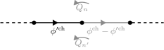
Figure 11: In order to describe the presence of external fluxes, each chord branch of the circuit (solid lines) is split into two branches, one representing the original element (black solid line), the other representing the electromotive force (solid gray line). As a consequence, the total flux $\phi^{\text{ch}}$ along the elements splits into the flux $\phi^{\prime\text{ch}}$ along the original element and the flux $\phi^{\text{ch}}-\phi^{\prime\text{ch}}$ along the virtual branch. Ensuring the Kirchhoff laws therefore requires adding the terms $-(Q_{n}-Q_{n^{\prime}})(\dot{\phi}^{\text{ch}}-\dot{\phi}^{\prime\text{ch}})=-q^{\text{ch}}(\dot{\phi}^{\text{ch}}-\dot{\phi}^{\prime\text{ch}})$ with the chord charge $q^{\text{ch}}=Q_{n}-Q_{n^{\prime}}$ to the Lagrangian.

Appendix D Proof of the rules for the inclusion of external fluxes using the mixed formulation

In this section, we want to show that the mixed formulation allows to understand the origin of the rules for the inclusion of external fluxes into the node flux formulation that were given in Ref. devoret:96, .

To that end, let us assume the presence of fluxes $\bm{\Phi}^{\text{ex}}$ in the loops corresponding to the loop charges $\bm{Q}$. We split each chord of the circuit graph into two branches, one which represents the original chord element and a second virtual branch which represents the electromotive force due to the external flux. As a consequence of the splitting, the total flux $\bm{\phi}^{\text{ch}}$ over the chord and the virtual branch will split up into a flux $\bm{\phi}^{\prime\text{ch}}$ over the chord element and a flux $\bm{\phi}^{\text{ch}}-\bm{\phi}^{\prime\text{ch}}$ over the virtual branch. Describing the virtual element in terms of charges requires adding the terms $\dot{\bm{Q}}\cdot\bm{\Phi}^{\text{ex}}-\bm{q}^{\text{ch}}\cdot(\dot{\bm{\phi}}^{\text{ch}}-\dot{\bm{\phi}}^{\prime\text{ch}})$ to the Lagrangian, c.f. Fig. 11. As discussed in App. A, the chord charges $\bm{q}^{\text{ch}}$ are related to the loop charges $\bm{Q}$ according to $\bm{q}^{\text{ch}}=B_{\text{ch}}^{T}\bm{Q}$ with the invertible matrix $B_{\text{ch}}$. Since the loop charges $\bm{Q}$ are not dynamic, their equations of motion yield a constraint $\dot{\bm{\phi}}^{\prime\text{ch}}=\dot{\bm{\phi}}^{\text{ch}}+B_{\text{ch}}^{-1}\dot{\bm{\phi}}^{\text{ex}}$.

For a chord $b$ with an orientation that is consistent (inconsistent) with the counter-clockwise orientation of its corresponding chord loop, the entries $(B_{\text{ch}}^{-1})_{bl}$ are given by $+1$ ($-1$) for all loops that lie within the face having the chord loop as its boundary and zero for all other loops. That means that all the non-zero entries in the rows of $B^{-1}_{\text{ch}}$ are of absolute value $1$ and have the same sign. To see that this description of the entries yields indeed the inverse of $B_{\text{ch}}$, let us consider the expression

$$M_{bb^{\prime}}=\sum_{l}(B^{-1}_{\text{ch}})_{bl}(B_{\text{ch}})_{lb^{\prime}}.$$ (45)

We need to show that $M_{bb^{\prime}}=\delta_{bb^{\prime}}$. When $b\neq b^{\prime}$, the chord $b^{\prime}$ lies either outside or inside the face having the chord loop corresponding to $b$ as its boundary. It cannot lie on the boundary of the face, i.e., it cannot be a part of the chord loop corresponding to $b$, since the chords uniquely specify a loop in the graph. If it lies outside the face, we obtain $M_{bb^{\prime}}=0$ by our characterization of the matrix $B_{\text{ch}}^{-1}$. If it lies inside the face, it forms part of two neighboring loops $l$, $l^{\prime}$ whose entries $(B_{\text{ch}})_{lb^{\prime}}$, $(B_{\text{ch}})_{l^{\prime}b^{\prime}}$ differ in sign. Since the rows of $B_{\text{ch}}^{-1}$ all have the same sign we also obtain $M_{bb^{\prime}}=0$ upon summing over $l$. For $b=b^{\prime}$, there is only one loop $l$ which lies in the face having the chord loop corresponding to $b$ as its boundary, and the entries $(B_{\text{ch}}^{-1})_{bl}$, $(B_{\text{ch}})_{bl}$ are both either plus or minus one, giving $M_{bb}=1$. Therefore, $M_{bb^{\prime}}=\delta_{bb^{\prime}}$. This shows that we may simply work with the original circuit graph without the virtual branches, provided we add to each expression involving the flux in a chord the external flux in its corresponding loop devoret:96 .

Appendix E Additional example for the mixed formulation

Figure 12: Circuit corresponding to the setup in Ref. vogt:15, . We only want to describe the Josephson junction (the subgraph complement depicted in black) in terms of node fluxes, whereas we describe the rest of the circuit (the subgraph depicted in gray) in terms of loop charges.

As an example, consider the circuit depicted in Fig. 12 which corresponds to the setup studied in Ref. vogt:15, . According to the rules discussed in the main text, its Lagrangian reads

$$\mathcal{L}=\sum_{i=1}^{N}\Bigl{[}\frac{1}{2L_{0}}\dot{Q}_{i}^{2}-\frac{1}{2C_{J}}Q_{i}^{\prime 2}-\frac{1}{2C_{0}}(Q_{i}-Q_{i+1})^{2}$$

$$+E_{J}\cos(2\pi\varphi_{i}/\Phi_{Q})-(Q_{i}^{\prime}-Q_{i})\dot{\varphi}_{i}\Bigr{]},$$ (46)

where we have defined $Q_{N+1}=0$ and $\varphi_{i}=\phi_{i}-\phi_{i^{\prime}}$. Note that the last term $-(Q_{i}^{\prime}-Q_{i})\dot{\varphi}_{i}$ just corresponds to the term $-\sum_{i}Q^{\partial}_{i}\sum_{j}\dot{\phi}_{ij}$ that appears in the mixed formulation as discussed in the main text. Note that the term $\dot{\varphi}_{i}Q_{i}$ enters with an overall plus sign since the voltage drop $\dot{\varphi}_{i}$ is measured in the direction opposite to the anticlockwise orientation of the loop current $Q_{i}$. There is no kinetic term for the coordinates $Q_{i}^{\prime}$ such that their Euler-Lagrange equations are algebraic with the solution $Q_{i}^{\prime}=-C_{J}\dot{\varphi}_{i}$. Inserting this solution back into the Lagrangian and performing the Legendre transformation with respect to $\dot{\varphi}_{i}$ and $\dot{Q}_{i}$ yields the Hamiltonian

$$H=\sum_{i=1}^{N}\Bigl{[}\frac{1}{2C_{J}}(q_{i}-Q_{i})^{2}-E_{J}\cos(2\pi\varphi_{i}/\Phi_{Q})$$

$$+\frac{1}{2C_{0}}(Q_{i}-Q_{i+1})^{2}+\frac{1}{2L_{0}}\Phi_{i}^{2}\Bigr{]},$$ (47)

where $(q_{i},\varphi_{i})$ and ($\Phi_{i},Q_{i})$ are canonically conjugate pairs. Eq. (E) reproduces the result derived in Ref. vogt:15, .

Appendix F Diagonalization of fluxonium using a higher-order matrix Numerov method

An efficient way of diagonalizing the fluxonium Hamiltonian consists in projecting the Hamiltonian onto the eigenstates of the harmonic part due to charging energy and inductive shunt, and diagonalizing the resulting matrix. The disadvantage of this method is the fact that it requires calculating explicitly all matrix elements of the cosine potential using the harmonic oscillator eigenstates. This can be done analytically but the resulting expressions are quite involved. A more direct approach, which is simpler in practice, consists in diagonalizing the Hamiltonian in real space. This requires discretizing the second-order derivative operator. For this, one usually employs the lowest-order Numerov approximation of order $\mathcal{O}(a^{4})$, where $a$ is the lattice spacing. The resulting discretized Schroedinger equation can be recast in matrix form pillai:12 such that it can be conveniently solved by standard (sparse) matrix methods. It would seem natural to consider also higher-order Numerov representations of the second-order derivative of order $\mathcal{O}(a^{2r+2})$, where $r\in\mathbb{N}$, but they are normally avoided due to stability issues blatt:67 . Interestingly, we have found that stability is not a problem when solving the resulting eigenvalue problem by standard (sparse) matrix methods instead of the conventional shooting method; a method that will be described in the following.

We consider at time-independent Schroedinger equation of the form

$$D^{2}\psi(x)=\bigl{[}-i\partial_{x}+A(x)\bigr{]}^{2}\psi(x)=-f(x)\psi(x),$$ (48)

where $D=-i\partial_{x}+A(x)$ is the covariant derivative operator and $f(x)$ equals $f(x)=2m[V(x)-E]$ for a Hamiltonian of the standard form $H=(p+A)^{2}/2m+V(x)$. For a wave function $\tilde{\psi}(x)$ defined as

$$\tilde{\psi}(x)=e^{i\int^{x}dx^{\prime}\,A(x^{\prime})}\psi(x),$$ (49)

we find the relation

$$e^{-i\int^{x}dx^{\prime}\,A(x^{\prime})}(-i\partial_{x})^{n}\tilde{\psi}(x)=D^{n}\psi(x),$$ (50)

which gives a convenient way of evaluating the higher orders of the covariant derivative acting on $\psi(x)$ through conventional derivatives of $\tilde{\psi}(x)$. Using Eq. (50), we obtain through Taylor expansion with respect to $\lambda$ the result

$$e^{-i\int^{x}dx^{\prime}\,A(x^{\prime})}\bigl{[}\tilde{\psi}(x+\lambda)+\tilde{\psi}(x-\lambda)\bigr{]}$$

$$=\psi(x+\lambda)e^{i\int_{x}^{x+\lambda}dx^{\prime}A(x^{\prime})}+\psi(x-\lambda)e^{-i\int_{x-\lambda}^{x}dx^{\prime}A(x^{\prime})}$$

$$=\sum_{n=0}^{\infty}\frac{2(-1)^{n}}{(2n)!}D^{2n}\psi(x)\lambda^{2n},$$ (51)

which gives a relation between the values of the covariant derivatives $D^{2j}\psi(x)$, $j\in\mathbb{N}_{0}$, and the value of the wave function $\psi(x)$ at positions $x\pm\lambda$. Following ideas of Ref. tang:14, , we stop the expansion (F) at $n=r$ and evaluate (F) for values $\lambda=ja$, $j\in\{-r,\dots,r\}\setminus\{0\}$, where $a$ is the lattice constant, which gives $2r$ equations for the covariant derivative $D^{2j}\psi(x)$ and the wave function values at points $\psi(x+ja)$. Solving these equations for $D^{2}\psi(x)$ and $D^{2r}\psi(x)$ yields expansions of the form

$$D^{2}\psi(x) =\frac{1}{a^{2}}\sum_{j=-r}^{j=r}c_{j}\psi_{j}+\mathcal{O}(a^{2r})$$ (52)

$$D^{2r}\psi(x) =\frac{1}{a^{2r}}\sum_{j=-r}^{j=r}d_{j}\psi_{j}+\mathcal{O}(a^{2}),$$ (53)

where we introduced the abbreviated notation $\psi_{j}=\psi(x+ja)$. The expansion coefficients $c_{j}$ and $d_{j}$ read

$$c_{j} =\sum_{k=1}^{r}\frac{2r^{2}((r-1)!)^{2}}{(r-k)!(r+k)!}\frac{(-1)^{k}}{k^{2}}\biggl{(}-2\delta_{j,0}$$

$$\qquad\qquad\qquad\qquad\qquad+\delta_{k,|j|}e^{i\int_{x}^{x+ja}dx^{\prime}A(x^{\prime})}\biggr{)},$$ (54)

$$d_{j} =\frac{(-1)^{|j|}(2r)!}{(r-|j|)!(r+|j|)!}e^{i\int_{x}^{x+ja}dx^{\prime}A(x^{\prime})}.$$ (55)

Numerov’s idea is to improve the accuracy of the expansion by a factor of $a^{2}$ by exploiting the structure of the differential equation (48). Including the term of order $\lambda^{2n+2}$ in Eq. (F) (that we previously dropped in order to arrive at Eq. (52)) and solving for the unknowns $D^{2j}\psi(x)$ with $j\in\{1,\dots,r\}$ while keeping $D^{2r+2}\psi(x)$ as a free parameter yields

$$D^{2}\psi(x) =\frac{1}{a^{2}}\sum_{j=-r}^{r}c_{j}\psi_{j}+\frac{(r!)^{2}a^{2r}D^{2r+2}\psi(x)}{(2r+1)!(r+1)}$$

$$\qquad+\mathcal{O}(a^{2r+2}).$$ (56)

Acting on both sides of Eq. (48) with $D^{2r}$ gives the expression

$$D^{2r+2}\psi(x)=-D^{2r}\bigl{[}f(x)\psi(x)\bigr{]}$$ (57)

for $D^{2r+2}\psi(x)$. Since we only need $D^{2r}[f(x)\psi(x)]$ to accuracy $\mathcal{O}(a^{2})$ in the expansion (F) of order $\mathcal{O}(a^{2r+2})$, we can use the previously derived expression (53). We then obtain the Numerov’s expression for the second-order covariant derivative

$$D^{2}\psi(x)=\frac{1}{a^{2}}\sum_{j=-r}^{r}c_{j}\psi_{j}-\frac{(r!)^{2}}{(2r+1)!(r+1)}$$

$$\times\sum_{j=-r}^{r}d_{j}f_{j}\psi_{j}+\mathcal{O}(a^{2r+2}),$$ (58)

which is better by a factor of $a^{2}$ in accuracy compared to the naive form (52).

Extending ideas of Ref. pillai:12, , we can convert this system of equations into a generalized eigenvalue problem. We introduce a matrix $A$ having $c_{j}/a^{2}$ on the $j$-th diagonal, where $j>0$ refers to the upper diagonals and $j<0$ refers to the lower diagonals, a diagonal matrix $V=\mathop{\rm diag}(V_{j})$ representing the potential, and a matrix $B$ having $-(r!)^{2}d_{j}/(2r+1)!(r+1)$ on the $j$-th diagonal. All of these matrices are sparse and allow writing Eq. (48) as the sparse generalized eigenvalue problem

$$\biggl{[}\frac{1}{2m}A+(B+1)V\biggr{]}\bm{\psi}=EB\bm{\psi},$$ (59)

where $\bm{\psi}$ is the discretized wave function vector. This Hermitian generalized eigenvalue problem can be solved efficiently by standard methods.

References

- (1) N. A. Masluk, I. M. Pop, A. Kamal, Z. K. Minev, and M. H. Devoret, Implementation of low-loss superinductances for quantum circuits, Phys. Rev. Lett. 109, 137002 (2012).
- (2) A. Kitaev, Protected qubit based on a superconducting current mirror, cond-mat/0609441 (2006).
- (3) V. E. Manucharyan, J. Koch, L. Glazman, and M. Devoret, Fluxonium: single Cooper pair circuit free of charge offsets, Science 326, 113 (2009).
- (4) M. Tinkham, Introduction to Superconductivity, 2nd edition (McGraw-Hill, New York, 1996).
- (5) J. E. Mooij and Y. V. Nazarov, Superconducting nanowires as quantum phase-slip junctions, Nat. Phys. 2, 169 (2006).
- (6) K. Y. Arutyunov, D. S. Golubev, and A. D. Zaikin, Superconductivity in one dimension, Phys. Rep. 464, 1 (2008).
- (7) O. V. Astafiev, L. B. Ioffe, S. Kafanov, Y. A. Pashkin, K. Y. Arutyunov, D. Shahar, O. Cohen, and J. S. Tsai, Coherent quantum phase slip, Nature (London) 484, 355 (2012).
- (8) J. T. Peltonen, O. V. Astafiev, Y. P. Korneeva, B. M. Voronov, A. A. Korneev, I. M. Charaev, A. V. Semenov, G. N. Golt’sman, L. B. Ioffe, T. M. Klapwijk, and J. S. Tsai, Coherent flux tunneling through nbn nanowires, Phys. Rev. B 88, 220506 (2013).
- (9) A. Belkin, M. Brenner, T. Aref, J. Ku, and A. Bezryadin, Little-Parks oscillations at low temperatures: Gigahertz resonator method, App. Phys. Lett. 98, 242504 (2011).
- (10) A. Belkin, M. Belkin, V. Vakaryuk, S. Khlebnikov, and A. Bezryadin, Formation of quantum phase slip pairs in superconducting nanowires, Phys. Rev. X 5, 021023 (2015).
- (11) J. M. Fink, M. Kalaee, A. Pitanti, R. Norte, L. Heinzle, M. Davanco, K. Srinivasan, and O. Painter, Quantum electromechanics on silicon nitride nanomembranes, Nat. Commun. 7, 12396 (2016).
- (12) N. Samkharadze, A. Bruno, P. Scarlino, G. Zheng, D. P. DiVincenzo, L. DiCarlo, and L. M. K. Vandersypen, High kinetic inductance superconducting nanowire resonators for circuit QED in a magnetic field, Phys. Rev. Appl. 5, 044004 (2016).
- (13) B. Yurke and J. S. Denker, Quantum network theory, Phys. Rev. A 29, 1419 (1984).
- (14) M. H. Devoret, Quantum Fluctuations in Electrical Circuits, in Les Houches Session LXIII, edited by S. Reynaud, E. Giacobino, and J. Zinn-Justin (Elsevier, Amsterdam, 1996).
- (15) D. A. Ivanov, L. B. Ioffe, V. B. Geshkenbein, and G. Blatter, Interference effects in isolated Josephson junction arrays with geometric symmetries, Phys. Rev. B 65, 024509 (2001).
- (16) J. R. Friedman and D. V. Averin, Aharonov-Casher-effect suppression of macroscopic tunneling of magnetic flux, Phys. Rev. Lett. 88, 050403 (2002).
- (17) J. C. Maxwell, A Treatise On Electricity And Magnetism, 3 ed. (Clarendon Press, Oxford, 1892).
- (18) E. Shragowitz and E. Gerlovin, The set of Lagrange and Routh formulations for non-linear networks, Int. J. Circ. Theor. App. 16, 129 (1988).
- (19) H. Kwatny, F. Massimo, and L. Bahar, The generalized Lagrange formulation for nonlinear RLC networks, IEEE Trans. Circuits Syst. 29 (4), 220 (1982).
- (20) L. O. Chua and J. McPherson, Explicit topological formulation of Lagrangian and Hamiltonian equations for nonlinear networks, IEEE Trans. Circuits Syst. 21, 277 (1974).
- (21) A. MacFarlane, Dual-system methods in dynamical analysis. part 1: Variational principles and their application to nonlinear-network theory, Proc. IEEE 116, 1453 (1969).
- (22) L. Weiss and W. Mathis, A Hamiltonian formulation for complete nonlinear RLC-networks, IEEE Trans. Circuits Syst. 44, 843 (1997).
- (23) H. Massimo, F.M.and Kwatny and L. Bahar, Derivation of the Brayton-Moser equations from a topological mixed potential function, J. Franklin Inst. 310, 259 (1980).
- (24) N. Bakhvalov, G. Kazacha, K. Likharev, and S. Serdyukova, Single-electron solitons in one-dimensional tunnel structures, JETP 68, 581 (1989).
- (25) Z. Hermon, E. Ben-Jacob, and G. Schön, Charge solitons in 1-D arrays of serially coupled Josephson junctions, Phys. Rev. B 54, 1234 (1996).
- (26) D. B. Haviland and P. Delsing, Cooper-pair charge solitons: The electrodynamics of localized charge in a superconductor, Phys. Rev. B 54, R6857(R) (1996).
- (27) J. Homfeld, I. Protopopov, S. Rachel, and A. Shnirman, Charge solitons and their dynamical mass in one-dimensional arrays of josephson junctions, Phys. Rev. B 83, 064517 (2011).
- (28) N. Vogt, R. Schäfer, H. Rotzinger, W. Cui, A. Fiebig, A. Shnirman, and A. V. Ustinov, One-dimensional Josephson junction arrays: Lifting the Coulomb blockade by depinning, Phys. Rev. B 92, 045435 (2015).
- (29) G. Burkard, R. H. Koch, and D. P. DiVincenzo, Multi-level quantum description of decoherence in superconducting qubits, Phys. Rev. B 69, 064503 (2004).
- (30) G. Burkard, Circuit theory for decoherence in superconducting charge qubits, Phys. Rev. B 71, 144511 (2005).
- (31) Remember that counts the charge on one of the capacitor plates while the capacitor itself is overall charge neutral. Current flows may thus change without violating charge conservation.
- (32) J. Koch, V. Manucharyan, M. H. Devoret, and L. I. Glazman, Charging effects in the inductively shunted Josephson junction, Phys. Rev. Lett. 103, 217004 (2009).
- (33) K. Thulasiraman and M. Swamy, Graphs: Theory and Algorithms (Wiley, Hoboken, 1992).
- (34) W. Guichard and F. W. J. Hekking, Phase-charge duality in Josephson junction circuits: Role of inertia and effect of microwave irradiation, Phys. Rev. B 81, 064508 (2010).
- (35) A. J. Kerman, Flux-charge duality and topological quantum phase fluctuations in quasi-one-dimensional superconductors, New J. Phys. 15, 105017 (2013).
- (36) R. P. Feynman and A. R. Hibbs, Quantum Mechanics and Path Integrals (McGraw-Hill Book Company, New York, 1965).
- (37) R. Savit, Duality in field theory and statistical systems, Rev. Mod. Phys. 52, 453 (1980).
- (38) J. D. Jackson, Classical Electrodynamics, 3rd edition (Wiley, Hoboken, 1999).
- (39) The presence of this loop can be rationalized by imagining an embedding of the circuit on the surface of a sphere.
- (40) S. E. Nigg, H. Paik, B. Vlastakis, G. Kirchmair, S. Shankar, L. Frunzio, M. Devoret, R. Schoelkopf, and S. Girvin, Black-box superconducting circuit quantization, Phys. Rev. Lett. 108, 240502 (2012).
- (41) J. Bourassa, F. Beaudoin, J. M. Gambetta, and A. Blais, Josephson junction-embedded transmission-line resonators: from Kerr medium to in-line transmon, Phys. Rev. A 86, 013814 (2012).
- (42) M. Leib, F. Deppe, A. Marx, R. Gross, and M. Hartmann, Networks of nonlinear superconducting transmission line resonators, New J. Phys. 14, 075024 (2012).
- (43) F. Solgun, D. W. Abraham, and D. P. DiVincenzo, Blackbox quantization of superconducting circuits using exact impedance synthesis, Phys. Rev. B 90, 134504 (2014).
- (44) F. Solgun and D. DiVincenzo, Multiport impedance quantization, Ann. Phys. 361, 605 (2015).
- (45) R. P. Feynman and F. L. Vernon, Jr., The theory of a general quantum system interacting with a linear dissipative system, Ann. Phys. (NY) 24, 118 (1963).
- (46) A. O. Caldeira and A. J. Leggett, Quantum tunneling in a dissipative system, Ann. Phys. (NY) 149, 374 (1983).
- (47) G. Schön and A. D. Zaikin, Quantum coherent effects, phase transitions, and the dissipative dynamics of ultra small tunnel junctions, Phys. Rep. 198, 237 (1990).
- (48) A. Schmid, Diffusion and localization in a dissipative quantum system, Phys. Rev. Lett. 51, 1506 (1983).
- (49) S. A. Bulgadaev, Phase diagram of a dissipative quantum system, JETP Lett. 39, 315 (1984).
- (50) F. Guinea, V. Hakim, and A. Muramatsu, Diffusion and localization of a particle in a periodic potential coupled to a dissipative environment, Phys. Rev. Lett. 54, 263 (1985).
- (51) A. Kamenev, Field theory of non-equilibrium systems (Cambridge University Press, Cambridge, 2011).
- (52) W.-K. Chen, Graph Theory and Its Engineering Applications, Advanced series in electrical and computer engineering (World Scientific, Singapore, 1997).
- (53) S. M. Apenko, Environment-induced decompactification of phase in Josephson junctions, Phys. Lett. A 142, 277 (1989).
- (54) A. Zaikin, Quantum dynamics of the charge in Josephson tunnel junctions, J. Low Temp. Phys. 80, 223 (1990).
- (55) In principle, we could have but just corresponds to a redefinition of the external flux .
- (56) A. Böhm, H. Koizumi, Q. Niu, J. Zwanziger, and A. Mostafazadeh, The Geometric Phase in Quantum Systems (Springer, Berlin, 2003).
- (57) A. B. Zorin, Bloch inductance in small-capacitance Josephson junctions, Phys. Rev. Lett. 96, 167001 (2006).
- (58) Yu. Makhlin, G. Schön, and A. Shnirman, Quantum-state engineering with Josephson-junction devices, Rev. Mod. Phys. 73, 357 (2001).
- (59) R. J. Schoelkopf, A. A. Clerk, S. M. Girvin, K. W. Lehnert, and M. H. Devoret, Qubits as spectrometers of quantum noise, in Quantum Noise in Mesoscopic Physics, edited by Y. V. Nazarov, vol. 97 of Nato Science Series II, pp. 175–203 (Springer Netherlands, AZ Dordrecht, 2003).
- (60) B. Douçot and J. Vidal, Pairing of Cooper pairs in a fully frustrated Josephson junction chain, Phys. Rev. Lett. 88, 227005 (2002).
- (61) B. Douçot and L. Ioffe, Physical implementation of protected qubits, Rep. Prog. Phys. 75, 072001 (2012).
- (62) M. T. Bell, J. Paramanandam, L. B. Ioffe, and M. E. Gershenson, Protected josephson rhombi chains, Phys. Rev. Lett. 112, 167001 (2014).
- (63) J. Koch, T. M. Yu, J. Gambetta, A. A. Houck, D. I. Schuster, J. Majer, A. Blais, M. H. Devoret, S. M. Girvin, and R. J. Schoelkopf, Charge insensitive qubit design derived from the Cooper pair box, Phys. Rev. A 76, 042319 (2007).
- (64) A. Yu. Kitaev, Unpaired Majorana fermions in quantum wires, Phys.-Usp. 44, 131 (2001), cond-mat/0010440.
- (65) B. van Heck, F. Hassler, A. R. Akhmerov, and C. W. J. Beenakker, Coulomb stability of the -periodic Josephson effect of Majorana fermions, Phys. Rev. B 84, 180502(R) (2011).
- (66) C. W. J. Beenakker, Search for Majorana fermions in superconductors, Annu. Rev. Con. Mat. Phys. 4, 113 (2013).
- (67) T. D. Stanescu and S. Tewari, Majorana fermions in semiconductor nanowires: Fundamentals, modeling, and experiment, J. Phys.: Condens. Matter 25, 233201 (2013).
- (68) M. Pillai, J. Goglio, and T. Walker, Matrix Numerov method for solving Schroedinger’s equation, Am. J. Phys. 80, 1017 (2012).
- (69) J. M. Blatt, Practical points concerning the solution of the Schrödinger equation, J. Comput. Phys. 1, 382 (1967).
- (70) D. Tang, B.Sc. Thesis, National University of Singapore, 2014.