Thermodynamic and spectral properties of adiabatic Peierls chains

Abstract

We present exact numerical results for the effects of thermal fluctuations on the experimentally relevant thermodynamic and spectral properties of Peierls chains. To this end, a combination of classical Monte Carlo sampling and exact diagonalization is used to study adiabatic half-filled Holstein and Su-Schrieffer-Heeger models. The classical nature of the lattice displacements in combination with parallel tempering permit simulations on large system sizes and a direct calculation of spectral functions in the frequency domain. Most notably, the long-range order and the associated Peierls gap give rise to a distinct low-temperature peak in the specific heat. The closing of the gap and suppression of order by thermal fluctuations involves in-gap excitations in the form of soliton-antisoliton pairs, and is also reflected in the dynamic density and bond structure factors as well as in the optical conductivity. We compare our data to the widely used mean-field approximation, and highlight relations to symmetry-protected topological phases and disorder problems.

I Introduction

Quasi-one-dimensional (1D) materials exhibit exciting phenomena such as spin-charge separation due to electron-electron interaction (e.g., in TTF-TCNQ [1]) or insulating charge-density-wave states as a result of electron-phonon coupling (e.g., in blue bronze [2]). While the ground-state properties of 1D spin or electron models can often be fully understood with the help of bosonization [3] and numerical methods, models with phonons remain a challenge. The calculation of thermodynamic or nonequilibrium properties is even harder and requires further methodological improvements. The role of electron-phonon coupling for the relaxation of charge-density-wave systems after photo-induced phase transitions is currently of particular interest [4].

Because of the Peierls instability, a 1D metal with one electron per unit cell can undergo a transition to a dimerized state with long-range charge order and a gap at the Fermi level [5; 6]. Depending on the form of the coupling, the charge order is either on the sites or the bonds. Even neglecting electron-electron interaction, the Peierls state is affected by quantum fluctuations, soliton excitations, and thermal fluctuations, which makes exact theoretical descriptions highly nontrivial. For reviews see Refs. [7; 8].

While finite critical temperatures arise from interchain coupling, the experimental observation of $T_{c}$ values much smaller than mean-field predictions [9] suggests that the latter is much smaller than intrachain couplings. Above a dimensional crossover temperature $T_{\text{3D}}\ll T_{c}$, 1D models such as the Holstein [10] and the Su-Schrieffer-Heeger (SSH) model [11] reviewed in Refs. [12; 13] can be used. Except for the spinful SSH model, quantum lattice fluctuations destroy the ordered state for a sufficiently weak electron-phonon coupling [14; 15]. Beyond the critical coupling, quantum fluctuations mainly reduce the dimerization [16; 17]. The ground-state properties have been characterized in terms of correlation functions and excitation spectra [12; 13], but open questions remain concerning critical couplings and Luttinger parameters [18].

The numerical calculation of thermodynamic properties or spectral functions at finite temperature, as studied experimentally [19; 20; 21; 22; 23], is much more difficult and limited by the large Hilbert space (for density-matrix renormalization group methods [24]) or the analytic continuation (for quantum Monte Carlo methods [12; 13]). A few results are available for spin-Peierls models [25; 26]. Interestingly, even the simpler case of classical phonons has only been studied at very low temperatures [27; 28]. It is routinely used in material-specific modeling of ground-state properties, and should provide a reliable description when the Peierls gap and/or the temperature are large compared to the phonon frequency [29].

Here, we systematically explore the temperature dependence of the specific heat and the excitation spectra of spinless Holstein and SSH models in the adiabatic limit. The latter provides the rare opportunity of obtaining exact numerical results on large systems, including exact high-resolution spectral functions. This allows a detailed, quantitative understanding of thermal fluctuations and a comparison to the widely used mean-field approximation for experimentally relevant quantities such as the specific heat and the single-particle spectral function [19; 20; 21; 22; 23].

The organization is as follows. In Sec. II we define the models and review their ground-state properties. The method is described in Sec. III. Results for thermodynamic and spectral properties are discussed in Sec. IV and Sec. V, respectively. Section VI contains our conclusions, and the Appendix discusses finite-size effects.

II Models

We study electrons in one dimension coupled to the lattice, as described by a Hamiltonian

$$\hat{H}=\hat{H}_{\mathrm{ph}}+\hat{H}_{\mathrm{el}}\,,$$ (1)

where $\hat{H}_{\mathrm{ph}}$ is the lattice contribution and $\hat{H}_{\mathrm{el}}$ contains the electronic and electron-phonon parts. In general, $\hat{H}_{\mathrm{ph}}$ depends on the lattice displacements $\hat{q}_{i}$ and momenta ${\hat{p}_{i}}$. In the adiabatic limit, the lattice is static and the displacements become classical variables $q_{i}$, allowing us to replace $\hat{H}_{\mathrm{ph}}\to{H}_{\mathrm{ph}}$ in Eq. (1). In the following, we define the Holstein and SSH models directly in this limit.

The spinless Holstein model [10] describes fermions coupled to harmonic oscillators with quadratic potential

$${H}_{\mathrm{ph}}=\frac{K}{2}\sum_{i}q_{i}^{2}$$ (2)

and spring constant $K$. The electronic part of the Hamiltonian is given by

$$\hat{H}_{\mathrm{el}}=-t\sum_{i}\left(\hat{c}^{\dagger}_{i}\hat{c}^{\vphantom{\dagger}}_{i+1}+\hat{c}^{\dagger}_{i+1}\hat{c}^{\vphantom{\dagger}}_{i}\right)+g\sum_{i}q_{i}\left(\hat{n}_{i}-1/2\right)\,.$$ (3)

The first term describes the nearest-neighbor hopping of spinless fermions with amplitude $t$, where $\hat{c}^{\dagger}_{i}$ ($\hat{c}^{\vphantom{\dagger}}_{i}$) creates (annihilates) a fermion at site $i$. In the second term, the displacement $q_{i}$ couples to the local fermion density $\hat{n}_{i}=\hat{c}^{\dagger}_{i}\hat{c}^{\vphantom{\dagger}}_{i}$ with coupling parameter $g$.

In the spinless SSH model [11], the lattice energy depends on the relative displacements of neighboring sites,

$${H}_{\mathrm{ph}}=\frac{K}{2}\sum_{i}\left(q_{i+1}-q_{i}\right)^{2}\,.$$ (4)

The electronic part,

$$\hat{H}_{\mathrm{el}}=\sum_{i}\left[-t+\alpha\left(q_{i+1}-q_{i}\right)\right]\left(\hat{c}^{\dagger}_{i}\hat{c}^{\vphantom{\dagger}}_{i+1}+\hat{c}^{\dagger}_{i+1}\hat{c}^{\vphantom{\dagger}}_{i}\right)\,,$$ (5)

describes the modulation of the hopping amplitude by the coupling of the lattice displacements to the bond density.

For both models, we introduce a dimensionless coupling parameter $\lambda$ by rescaling the displacement fields. For the Holstein model $\lambda=g^{2}/(4Kt)$, whereas for the SSH model $\lambda=\alpha^{2}/(Kt)$. We use $t$ as the unit of energy, set the lattice constant and $\hbar$ to one, and consider half-filling (one electron per two sites).

At zero temperature, the exact properties of both models can be obtained from mean-field theory [30; 14; 31]. For any $\lambda>0$, the Peierls instability leads to a dimerization of the lattice that is captured by the ansatz $q_{i}=(-1)^{i}\Delta/(2g)$ for the Holstein model and $q_{i}=(-1)^{i}\Delta/(8\alpha)$ for the SSH model. Here, $\Delta$ is the gap calculated self-consistently from the gap equation. The lattice dimerization is accompanied by charge-density-wave order in the Holstein model and bond-density-wave order in the SSH model. The order has periodicity $2k_{F}$, where $k_{F}=\pi/2$ is the Fermi momentum. Commensurability with the lattice pins the phase of the order parameter to $\pi$ [32], so that the ground state is twofold degenerate under $\Delta\to-\Delta$. While exact at $T=0$, mean-field theory predicts a finite Peierls transition temperature $T_{c}$, in violation of the Mermin-Wagner theorem [33]. The adiabatic limit is expected to capture the physics of the dimerized phase [29].

While the Holstein and the SSH model both describe Peierls insulators, important differences arise from their different symmetries. The mean-field SSH Hamiltonian is often considered as the simplest model of a symmetry-protected topological band insulator [34], as reviewed in Ref. [35]. It obeys time-reversal, particle-hole, and chiral symmetry. Explicitly, under time reversal, $\mathcal{T}\hat{c}_{j}\mathcal{T}^{-1}=\hat{c}_{j}$ with $\mathcal{T}\mathrm{i}\mathcal{T}^{-1}=-\mathrm{i}$, whereas for a particle-hole transformation $\mathcal{P}\hat{c}_{j}\mathcal{P}^{-1}=(-1)^{j}\hat{c}^{\dagger}_{j}$ with $\mathcal{P}\mathrm{i}\mathcal{P}^{-1}=\mathrm{i}$. The chiral symmetry operator is given by $\mathcal{C}=\mathcal{T}\mathcal{P}$. These symmetries put the SSH model into the so-called BDI class of the general classification of symmetry-protected topological phases [36; 37; 38] which in 1D allows for a nontrivial topological invariant. The two degenerate ground states of the SSH model belong to different topological sectors. The symmetry-protected zero-energy states of the topological phase are identical to the soliton excitations at domain walls introduced in Refs. [11; 39]. For periodic boundaries, domain walls can only occur as soliton-antisoliton pairs. Depending on their size, such pairs may form bound polaron states with nonzero energy [7]. The Hamiltonian of the Holstein model belongs to the AI symmetry class with broken chiral (and particle-hole) symmetry as a result of the density-displacement coupling. The two degenerate ground states are therefore trivial and do not support topologically protected zero-energy states at domain walls. Nevertheless, soliton-antisoliton pairs can exist and were reported in simulations of the quantum phonon case [40]. While the topological classification is strictly valid only at $T=0$, the electronic symmetries persist for any configuration of displacements generated by thermal fluctuations.

III Method

To solve the electron-phonon problem at finite temperatures, we used the Monte Carlo method of Ref. [27]. In the adiabatic limit, and using the notation of Ref. [41], the partition function of Hamiltonian (1) takes the form

$$Z=\int dq_{1}\,\,\dots\int dq_{L}\,e^{-\beta{H}_{\mathrm{ph}}}Z_{\mathrm{el}}[q_{1},\dots,q_{L}]\,,$$ (6)

where $Z_{\mathrm{el}}=\operatorname{Tr}\exp[-\beta(\hat{H}_{\mathrm{el}}-\mu\hat{N})]$ is the grand-canonical partition function of the electronic subsystem, $\beta=1/k_{\text{B}}T$ the inverse temperature, $\mu$ the chemical potential and $\hat{N}$ the total particle-number operator.

For each configuration $C=\{q_{1},\dots,q_{L}\}$ of the classical displacements, $\hat{H}_{\mathrm{el}}$ is a noninteracting Hamiltonian that can be diagonalized exactly. The Monte Carlo method of Ref. [27] samples the continuous space of displacement configurations $C$. Expectation values take the form

$$\left\langle\hat{O}\right\rangle=\sum_{C}W[C]\left\llangle\hat{O}\right\rrangle_{C}$$ (7)

with the weight of the configuration

$$W[C]=\frac{1}{Z}e^{-\beta{H}_{\mathrm{ph}}[C]}Z_{\mathrm{el}}[C]$$ (8)

and the corresponding value of the observable

$$\left\llangle\hat{O}\right\rrangle_{C}=\frac{1}{Z_{\mathrm{el}}[C]}\operatorname{Tr}\left\{e^{-\beta(\hat{H}_{\mathrm{el}}[C]-\mu\hat{N})}\hat{O}[C]\right\}\,.$$ (9)

The weight $W[C]$ is always positive and can be sampled using the Metropolis algorithm [42]. For each configuration, observables are calculated from Eq. (9). Both quantities are obtained from a diagonalization of the $L\times L$ matrix representation of $\hat{H}_{\mathrm{el}}[C]$ which dominates the computational complexity of the algorithm.

Technically, Monte Carlo simulations of Eq. (7) are related to disorder problems at finite temperature [29]. For each configuration $C$, we solve an Anderson model [43] with either diagonal (site) disorder for the Holstein model or off-diagonal (bond) disorder for the SSH model. In contrast to common disorder problems, the probability distribution $W[C]$ has a nontrivial dependence on $Z_{\mathrm{el}}[C]$. However, in the high-temperature limit, $Z_{\mathrm{el}}[C]\approx 1$ and $W[C]$ becomes a Gaussian distribution. We will revisit this analogy below.

III.1 Sampling

Simulations were started from random configurations which were then updated by randomly picking a single $q_{i}$ and proposing a change $\Delta q$. $\Delta q$ was drawn from a Gaussian distribution with variance $\sigma_{q}^{2}$. Because at high temperatures $W[C]$ is dominated by $\exp(-\beta{H}_{\mathrm{ph}}[C])$, $\sigma_{q}\sim\sqrt{T}$ is a natural choice. However, at low temperatures, the distribution of displacements evolves into a two-peak structure [44] and $\sigma_{q}\sim\sqrt{T}$ becomes too sharp. Therefore, for each temperature, we performed a warmup to estimate the actual distribution of displacements. At low temperatures, the algorithm suffers from long autocorrelation times, which were overcome by parallel tempering [45]. For each coupling parameter $\lambda$, the data shown were generated from a fixed temperature grid with at least $64$ points. A switch of configurations at adjacent temperatures was proposed every $500$ updates. We set $\mu=0$ for half-filling and simulated lattices of length $L=162$ with periodic boundary conditions.

III.2 Observables

In the following, we define the relevant static and dynamic observables. For each configuration $C$, they were calculated from the single-particle basis of $\hat{H}_{\mathrm{el}}[C]$ given by the eigenvalues $E_{\lambda}$ and eigenvectors $\ket{\lambda}$.

The specific heat $C_{V}$ was calculated via

$$C_{V}[C]=k_{\text{B}}\beta^{2}\left[\left\llangle\hat{H}^{2}\right\rrangle_{C}-\left\llangle\hat{H}\right\rrangle_{C}^{2}\right]\,.$$ (10)

To study the ordering of the electronic subsystem, we used the static structure factors

$$S_{\alpha}(q;C)=\frac{1}{L}\sum_{i,j}e^{\mathrm{i}q(i-j)}\left\llangle\hat{O}_{i}^{\alpha}\hat{O}_{j}^{\alpha}\right\rrangle_{C}$$ (11)

as a function of transferred momentum $q$. The subscript $\alpha=\rho$ ($\alpha=b$) denotes the charge (bond) structure factor. The corresponding operators $\hat{O}_{i}^{\alpha}$ are the local charge density $\hat{n}_{i}$ and bond density $\hat{B}_{i}=(\hat{c}^{\dagger}_{i}\hat{c}^{\vphantom{\dagger}}_{i+1}+\hat{c}^{\dagger}_{i+1}\hat{c}^{\vphantom{\dagger}}_{i})$.

Importantly, spectral functions can be calculated directly for real frequencies, without the need of numerical analytic continuation. For the single-particle spectral function $A(k,\omega)$, the Lehmann representation reads

$$A(k,\omega;C)=\sum_{\lambda}\left|\bra{0}\hat{c}^{\vphantom{\dagger}}_{k}\ket{\lambda}\right|^{2}\delta(\omega-E_{\lambda})\,.$$ (12)

From Eq. (12), the density of states $N(\omega)$ was obtained by summation over momentum $k$. Two-particle spectra were calculated from the dynamic structure factors

$$S_{\alpha}(q,\omega;C) =\Big{|}\sum_{\lambda}p_{\lambda}\bra{\lambda}\hat{O}_{q}^{\alpha}\ket{\lambda}\Big{|}^{2}\delta(\omega)$$ (13)

$$+\sum_{\lambda,\nu}p_{\nu}(1-p_{\lambda})\left|\bra{\lambda}\hat{O}_{q}^{\alpha}\ket{\nu}\right|^{2}\delta(E_{\lambda}-E_{\nu}-\omega)\,,$$

where $p_{\lambda}=\{\exp[\beta(E_{\lambda}-\mu)]+1\}^{-1}$ is the Fermi function and $\alpha=\rho,b$ as before. We also consider the real part of the optical conductivity

$$\sigma(\omega;C)=\sum_{\lambda,\nu}\frac{p_{\nu}-p_{\lambda}}{\omega}\left|\bra{\lambda}\hat{J}\ket{\nu}\right|^{2}\delta(E_{\lambda}-E_{\nu}-\omega)\,,$$ (14)

where $\hat{J}=\mathrm{i}\sum_{i}t_{i}(\hat{c}^{\dagger}_{i}\hat{c}^{\vphantom{\dagger}}_{i+1}-\hat{c}^{\dagger}_{i+1}\hat{c}^{\vphantom{\dagger}}_{i})$ is the current operator; here $t_{i}=t$ for the Holstein model and $t_{i}=t-\alpha(q_{i+1}-q_{i})$ for the SSH model, respectively.

Spectral functions were measured on a discrete frequency grid. Each data point represents the averaged spectral weight in an interval of width $\Delta\omega$. Unless stated otherwise we used $\Delta\omega=0.04t$.

IV Thermodynamics

We first discuss thermodynamic properties, focusing on the specific heat. The latter is an integrated quantity accessible to experiments that already captures the relevant temperature scales of the physical system.

Figure 1 shows the specific heat of both models as a function of temperature and for different couplings $\lambda$. For the large lattice size $L=162$ used, only minor finite-size effects appear (see Appendix). Note that adjacent data points in Fig. 1 are not statistically independent since they were generated by parallel tempering.

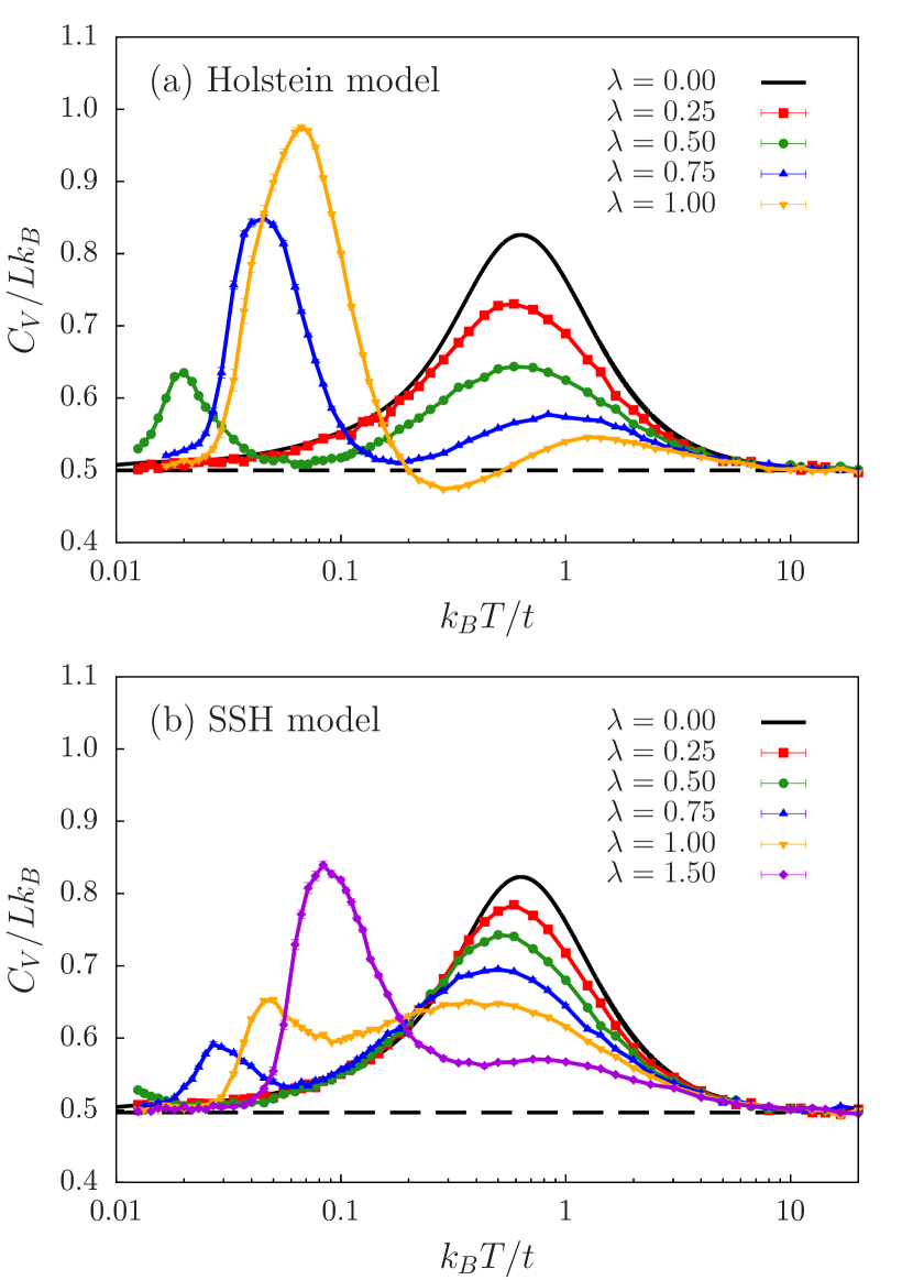
Figure 1: (Color online) Specific heat per site for (a) the Holstein and (b) the SSH model with $L=162$. The dashed lines indicate the respective free-phonon contributions.

At $\lambda=0$, the specific heat is the sum of contributions from the phonons and the electrons. In the adiabatic limit, the phonons are described by classical harmonic oscillators. According to the equipartition theorem, each phonon mode contributes $k_{\text{B}}/2$, which leads to the constant background in Fig. 1. (For the SSH model, the $k=0$ mode does not contribute because the length of the chain was fixed.) Therefore, $C_{V}$ does not vanish for $T\to 0$, in violation of the third law of thermodynamics. The electronic contribution reaches a maximum at the coherence temperature $k_{\text{B}}T\approx 0.63t$ and vanishes for $T\to 0$ and $T\to\infty$. The maximum is related to the thermal activation of charge fluctuations across the entire band width of our lattice model. The expected linear free-fermion contribution is visible in the interval $0.03t<k_{B}T<0.1t$ (for the system size $L=162$ used) in a different representation (not shown).

For $\lambda>0$, the electronic and phononic contributions to $C_{V}$ can no longer be separated. For the Holstein model, a small coupling $\lambda=0.25$ suppresses $C_{V}$ over the whole temperature range shown in Fig. 1(a). With increasing $\lambda$, the free-electron peak loses weight and shifts to higher temperatures. At $\lambda=1$ and intermediate temperatures, the specific heat even falls below the free-phonon contribution. For the SSH model, Fig. 1(b), $C_{V}$ is also suppressed at high temperatures, but its maximum shifts to slightly lower temperatures. Moreover, $C_{V}$ remains almost constant at intermediate temperatures.

For both models, an additional peak emerges in $C_{V}$ at low temperatures. While for small $\lambda$ the peak cannot be observed in the accessible temperature range, it shifts to higher temperatures and grows with increasing $\lambda$. This feature is robust against finite-size effects, only the downturn towards $T\to 0$ where the electronic contribution vanishes is not yet fully converged with $L$. For a detailed finite-size analysis see the Appendix.

The appearance of the low-temperature peak can be attributed to an enhancement of order as temperature is decreased. Figure 2 shows the static

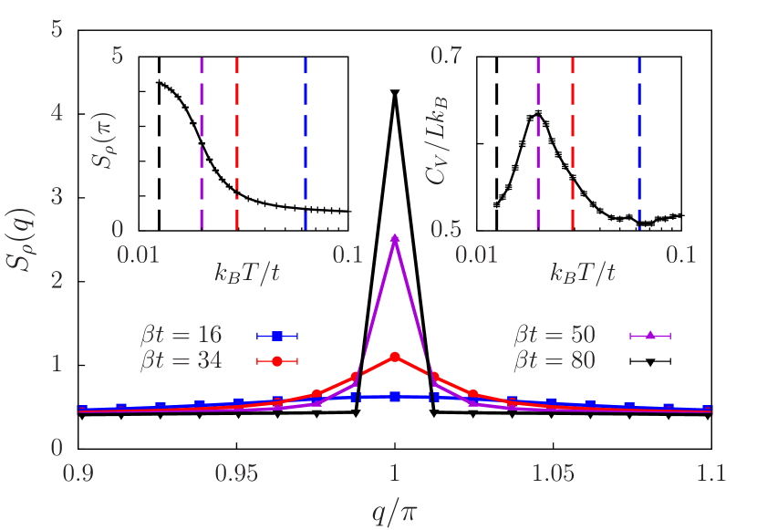
Figure 2: (Color online) Density structure factor $S_{\rho}(q)$ of the Holstein model around the ordering vector $q=2k_{F}=\pi$ for selected temperatures. The full temperature dependence of $S_{\rho}(\pi)$ is shown in the left inset. Dashed lines mark the temperatures for which $S_{\rho}(q)$ is shown in the main panel and match the evolution of the low-temperature peak in $C_{V}$, as shown in the right inset. Here, $\lambda=0.5$ and $L=162$.

density structure factor $S_{\rho}(q)$ for the Holstein model at $\lambda=0.5$. At low temperatures, $S_{\rho}(q)$ develops a peak at $q=2k_{F}=\pi$ that indicates the formation of a charge-density wave. Simultaneously, the peak in $C_{V}$ arises, as shown in the two insets of Fig. 2. Its maximum at $k_{\text{B}}T\simeq 0.02t$ corresponds with the inflection point of $S_{\rho}(\pi)$. The width of the peak is related to the temperature range where $2k_{F}$ correlations become prominent. The same behavior is expected for the SSH model and the bond structure factor $S_{b}(q)$.

While true long-range order only exists at $T=0$, the position of the low-temperature peak in $C_{V}$ can be regarded as a coherence scale at which pronounced $2k_{F}$ correlations set in and which marks the emergence of a clear Peierls energy gap. The thermal crossover is described by a correlation length $\xi(T)$ [46]. While $\xi(T)\to\infty$ for $T\to 0$, corresponding to long-range order, the correlation length is finite at $T>0$ where charge or bond correlations decay exponentially. Similar results have been obtained from a Ginzburg-Landau approach [47]. While a saddle-point approximation gives a second-order phase transition at a finite $T_{c}$ and a jump in $C_{V}$ [48], Scalapino et al. [47] used a functional method to treat fluctuations in the Ginzburg-Landau fields. Thereby, they mapped the 1D electron-phonon problem to a single quantum mechanical anharmonic oscillator [49]. In this approach, long-range order is destroyed at $T>0$, and $C_{V}$ is continuous with a peak similar to our results. The maximum in $C_{V}$ may be located well below the mean-field value for $T_{c}$ [49]. For the electron-phonon models considered here, the mean-field critical temperature is an order of magnitude larger than the peak positions in our $C_{V}$ data.

The results in Fig. 1 are very similar for the two models considered. With increasing $\lambda$, the free-electron contribution is suppressed and an additional low-temperature peak emerges that can be attributed to enhanced $2k_{F}$ charge or bond correlations, respectively. The same temperature scales will also be relevant for the spectral properties discussed in Sec. V. The relation between $C_{V}$ and the spectral function becomes apparent by considering the relation $C_{V}=\partial E_{\mathrm{tot}}/\partial T$ and using the equation of motion [50] to write the total energy as

$$E_{\mathrm{tot}}=\frac{N_{\mathrm{ph}}}{2\beta}+\sum_{k}\int_{-\infty}^{\infty}d\omega\,\frac{\omega+\epsilon_{k}}{2}\,n_{F}(\omega)\,A(k,\omega)\,.$$ (15)

Here, $N_{\mathrm{ph}}=L$ for the Holstein model and $N_{\mathrm{ph}}=L-1$ for the SSH model. According to Eq. (15), $E_{\mathrm{tot}}$ can be expressed as a sum rule of the single-particle spectrum weighted with the Fermi function $n_{F}(\omega)$ and the bare dispersion $\epsilon_{k}=-2t\cos k$. Thus, the specific heat measures the change of the density of states around the Fermi energy with temperature. The decrease of the free-electron peak in $C_{V}$ with increasing $\lambda$ therefore corresponds to a reduction of spectral weight across a broad region of energies and temperature, whereas the sharp low-temperature peak signals a sudden change in the single-particle spectrum. In particular, we will show that the emergence of the low-temperature peak is related to the Peierls gap.

V Spectral properties

In this section, we investigate how the temperature-driven suppression of $2k_{F}$ charge or bond order manifests itself in the single-particle and two-particle spectral functions [Eqs. (12)–(14)]. While at $T=0$ the spectral functions can be calculated exactly using mean-field theory, finite temperatures require numerical simulations.

V.1 Holstein model

For the Holstein model, the electron-phonon coupling is chosen as $\lambda=0.5$, for which the mean-field gap $\Delta\approx 0.68t$ and the interesting temperature scale set by the corresponding peak in $C_{V}$ is well accessible.

V.1.1 Temperature dependence of the density of states

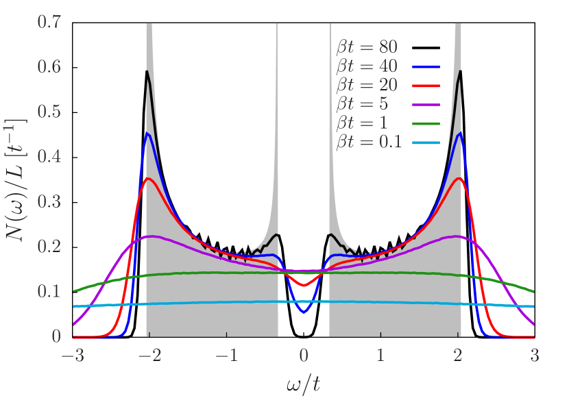
Figure 3: (Color online) Density of states of the Holstein model for $\lambda=0.5$ and $L=162$. The filled curve corresponds to the $T=0$ mean-field result (16).

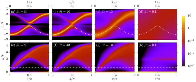
Figure 4: (Color online) (a)–(d) Single-particle spectral function $A(k,\omega)$ and (e)–(h) dynamic density structure factor $S_{\rho}(q,\omega)$ of the Holstein model for $\lambda=0.5$ and $L=162$. Dashed lines correspond to the $T=0$ mean-field dispersion and gap, respectively. For better visibility, the $\omega=0$ contributions to $S_{\rho}(q,\omega)$ are shown as a bar of width $0.1t$ in (e)–(h).

We begin with the density of states plotted in Fig. 3. The filled curve shows the exact mean-field result at $T=0$ which in the thermodynamic limit is given by

$$N(\omega)=\frac{L}{\pi}\frac{\left|\omega\right|}{\sqrt{\omega^{2}-\left(\frac{\Delta}{2}\right)^{2}}\sqrt{\left(2t\right)^{2}+\left(\frac{\Delta}{2}\right)^{2}-\omega^{2}}}$$ (16)

for $\Delta/2<\left|\omega\right|<\sqrt{(2t)^{2}+(\Delta/2)^{2}}$, and zero else. Hence, at the mean-field level, the electron-phonon interaction opens a gap $\Delta$ at the Fermi level and the shifts the upper edge of the band to higher energies. At the band edges, square-root singularities appear.

Thermal fluctuations lead to a broadening of the band edges and the singularities become finite peaks. At the lowest temperature considered in our simulation, $\beta t=80$, $N(\omega)$ is still close to the result at $T=0$, but spectral weight enters the mean-field gap exponentially. The fine structure visible in the middle of the bands is a finite-size effect and is partly smeared due to the use of a frequency grid with spacing $\Delta\omega$. With increasing temperature, the peak at the lower edge of the spectrum is strongly suppressed. At the same time, the $T=0$ gap is filled in and has disappeared at $\beta t=5$. At even higher temperatures, also the peak at the upper edge is entirely washed out. The weight is shifted to higher frequencies and the spectrum flattens completely.

The temperature of the gap closing in Fig. 3 coincides with the position of the low-temperature peak in $C_{V}$ and the suppression of $2k_{F}$ correlations in $S_{\rho}(q)$ in Fig. 2. According to Eq. (15), the change of $N(\omega)$ near the Fermi level is largest at the coherence scale $k_{\text{B}}T\approx 0.02t$ where $C_{V}$ has its maximum. Therefore, the peak in $C_{V}$ directly signals the formation of the gap. Its temperature scale is considerably lower than the mean-field gap $\Delta/2\approx 0.34t$ or the critical temperature $k_{\text{B}}T_{c}\approx 0.2t$, similar to the reduction of the transition temperature due to 1D fluctuations in Refs. [47; 51].

V.1.2 Momentum dependence of the spectral functions

The single-particle spectrum $A(k,\omega)$ and the dynamic density structure factor $S_{\rho}(q,\omega)$ are shown in Fig. 4. The temperatures were chosen to capture the interesting regions defined by the results for $C_{V}$ in Fig. 1.

For $\beta t=80$ [Fig. 4(a)], $A(k,\omega)$ closely follows the mean-field dispersion indicated by the dashed line. The imbalance of spectral weight between the original cosine dispersion and the shadow bands is characteristic for systems with competing periodicities and only disappears for $\lambda\to\infty$ [52]. Due to the finite temperature, the peaks in $A(k,\omega)$ are broadened and their positions deviate slightly from the mean-field dispersion at the band edges. There are additional features of minor weight that disperse from the edges of the original cosine band forming a continuum of excitations.

With increasing temperature [Fig. 4(b)], the broadening becomes larger and the shadow bands less pronounced. Inside the mean-field gap, two dispersing bands appear with dominant weight around $k_{\text{F}}=\pi/2$ (see also Sec. V.1.3). At $\beta t=10$ [Fig. 4(c)], the gap and the shadow bands have disappeared completely, and the locus of spectral weight follows the cosine dispersion of the noninteracting system. Further increasing the temperature only leads to a broadening of the spectrum until it becomes washed out completely, see Fig. 4(d).

Figures 4(e)–(h) show the dynamic density structure factor $S_{\rho}(q,\omega)$ at the same temperatures. At $\beta t=80$, $S_{\rho}(q,\omega)$ exhibits a particle-hole continuum but with a gap comparable to the mean-field gap (dashed line). Moreover, there is a sharp central (Bragg) peak at $q=2k_{F}=\pi$ associated with charge-density-wave order. At higher temperature [Figs. 4(f)–(g)], the edges of the particle-hole continuum diffuse, the gap is filled in, and the central peak becomes a Lorentzian of width $\xi^{-1}(T)$ in momentum space (cf. Fig. 2) where $\xi(T)$ is the correlation length introduced at the beginning of Sec. IV. In the high-temperature limit [Fig. 4(h)] the particle-hole continuum is washed out completely, and $S_{\rho}(q,\omega)$ contains (i) a spatially localized (i.e., $q$-independent) zero-energy Einstein phonon mode, and (ii) an additional mode at $\omega=2t$ related to the strong onsite disorder generated for the fermions by the lattice fluctuations (see Sec. V.3).

V.1.3 Closing of the single-particle gap

The closing of the single-particle gap in Fig. 4 is the result of two effects. First, a spatially homogeneous renormalization of the $T=0$ mean-field order parameter. Second, thermally induced defects in the lattice dimerization with energies below the band gap.

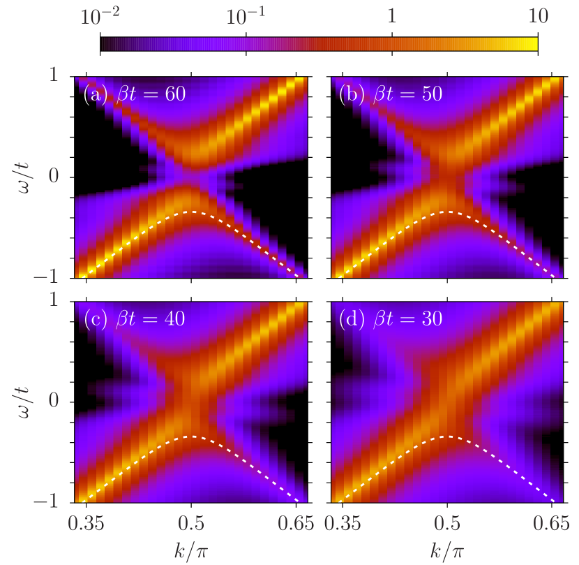
Figure 5: (Color online) Close-up of the single-particle spectral function $A(k,\omega)$ around $k_{F}=\pi/2$ for the same parameters as in Fig. 4. The dashed lines correspond to the mean-field dispersion at $T=0$. Here, we used a discretization $\Delta\omega=0.01t$.

A closeup of the thermally induced low-energy excitations is shown in Fig. 5. For $\beta t=60$ [Fig. 5(a)], we see a band above (below) the mean-field main band for $k<k_{F}$ ($k>k_{F}$), as well as a weaker band below (above) the mean-field shadow band for $k<k_{F}$ ($k>k_{F}$) that extends only over a small range of $k$ around $k_{F}$. Both features merge with the mean-field bands near $k_{F}$. With increasing temperature, the additional excitations gain spectral weight (especially close to $k_{F}$) and the feature following the shadow bands extends over a large $k$-range. Eventually, the gap is filled in and the linear dispersion near $k_{F}$ is restored, cf. Figs. 4(c) and 4(d).

At low temperatures [Fig. 4(a)], the spectral function has a close resemblance with that of the spinless Holstein model with quantum phonons [40]. The latter exhibits dispersive excitations with energy smaller than the mean-field gap that have been interpreted as polaron excitations. While quantum fluctuations reduce the minimal energy for polaron excitations [40], the latter coincides with the mean-field gap in the classical case [Fig. 4(a)].

V.1.4 Optical conductivity

Finally, we consider the optical conductivity $\sigma(\omega)$ in Fig. 6. At $T=0$, mean-field theory gives

$$\sigma(\omega)=\frac{L\Delta^{2}}{4\pi\omega^{2}}\sqrt{\frac{(4t)^{2}+\Delta^{2}-\omega^{2}}{\omega^{2}-\Delta^{2}}}$$ (17)

for $\Delta<\left|\omega\right|<\sqrt{(4t)^{2}+\Delta^{2}}$. The filled curve in Fig. 6 clearly shows the square-root singularity at the lower edge $\omega=\Delta$. In contrast to the density of states, there is no singularity at the upper edge where $\sigma(\omega)=0$. At $\beta t=80$, the lower edge of $\sigma(\omega)$ has already broadened significantly. As a function of temperature, we first observe a decrease of the optical gap due to the suppression of charge order. While this shift is qualitatively captured by a temperature-dependent mean-field gap $\Delta(T)$, the latter does not account for the nontrivial broadening due to fluctuations. Although the single-particle gap is filled in at high temperatures, there is no Drude peak. The absence of the latter, and the shift of the peak in $\sigma(\omega)$ back to larger frequencies for $\beta t\lesssim 20$, can be attributed to the onset of incoherence. In contrast, in the mean-field charge-density-wave approximation, $\Delta=0$ at $T>T_{c}$ so that the electrons can move coherently. At even higher temperatures, the strong lattice fluctuations act as essentially random disorder. A characteristic peak emerges at $\omega=2t$ that becomes more pronounced as temperature increases further. The relation to a disorder problem will be discussed in more detail in Sec. V.3.

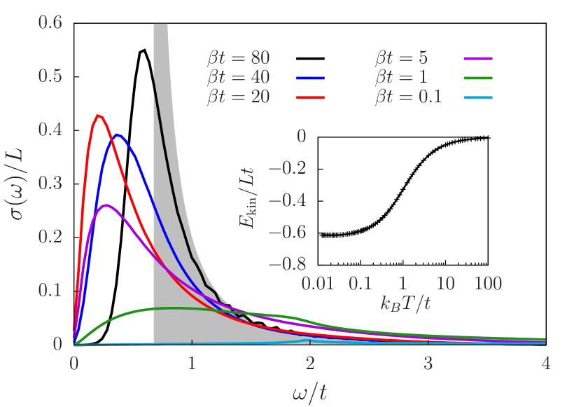
Figure 6: (Color online) Optical conductivity of the Holstein model for $\lambda=0.5$ and $L=162$. The filled curve is the $T=0$ mean-field result (17). The inset shows the kinetic energy of the electrons as a function of temperature. It is related to $\sigma(\omega)$ by the sum rule given in Eq. (18).

The integrated optical conductivity is related to the kinetic energy via the f-sum rule [53]

$$\int_{0}^{\infty}d\omega\,\sigma(\omega)=-\frac{\pi}{2}E_{\mathrm{kin}}\,.$$ (18)

The results for $E_{\text{kin}}$ in the inset of Fig. 6 reveal that up to $\beta t\approx 20$ spectral weight is merely redistributed, whereas it is significantly reduced at higher temperatures and vanishes for $T\to\infty$.

V.2 SSH model

The spectral properties of the SSH model are in many aspects similar to the Holstein model, and we therefore focus on the differences. To facilitate a comparison with the results for the Holstein model we take $\lambda=0.75$ for which the mean-field gap $\Delta\approx 0.76t$.

V.2.1 Temperature dependence of the density of states

Figure 7 shows the density of states, including the

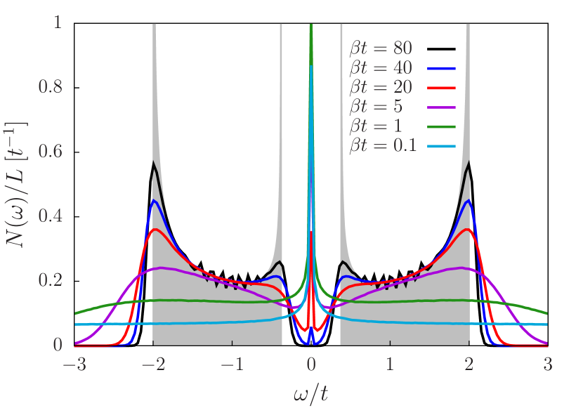
Figure 7: (Color online) Density of states of the SSH model for $\lambda=0.75$ and $L=162$. The filled curve corresponds to the $T=0$ mean-field result (19).

$T=0$ mean-field result given by

$$N(\omega)=\frac{L}{\pi}\frac{\left|\omega\right|}{\sqrt{\omega^{2}-\left(\frac{\Delta}{2}\right)^{2}}\sqrt{(2t)^{2}-\omega^{2}}}$$ (19)

for $\Delta/2<\left|\omega\right|<2t$, and zero otherwise. Equation (19) has the same form as Eq. (16), but the upper edge of the spectrum remains at $\omega=2t$ independent of $\lambda$. The temperature dependence of the mean-field bands, i.e., the broadening of the singularities and the closing of the gap, is similar to the Holstein model. However, there is an additional peak at $\omega=0$ that grows and broadens with increasing temperature. It survives even at the highest temperature considered where the rest of the spectrum has been completely washed out by thermal fluctuations. As discussed below, the peak is related to topologically protected midgap states of the SSH Hamiltonian.

V.2.2 Momentum dependence of the spectral functions

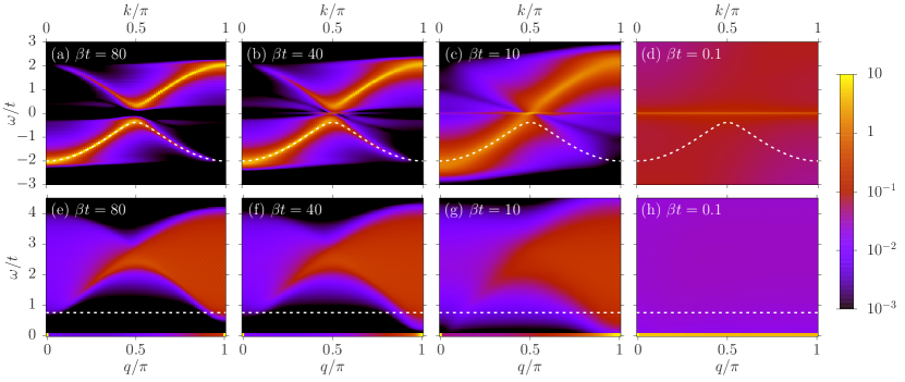
Figure 8: (Color online) (a)–(d) Single-particle spectral function $A(k,\omega)$ and (e)–(h) dynamic bond structure factor $S_{b}(q,\omega)$ of the SSH model for $\lambda=0.75$ and $L=162$. The dashed lines correspond to the $T=0$ mean-field dispersion and gap, respectively. For better visibility, the $\omega=0$ contributions to $S_{b}(q,\omega)$ are shown as a bar of width $0.1t$ in (e)–(h).

The single-particle spectral function $A(k,\omega)$ shown in Figs. 8(a)–(d) is again very similar to the Holstein model, except for the zero-energy peak. The latter is absent at $\beta t=80$ [Fig. 8(a)], where the spectrum closely follows the mean-field dispersion. It first emerges at $\beta t\simeq 40$ when the gap starts to be filled in by thermal excitations [Fig. 8(b)]. At $\beta t=10$ [Fig. 8(c)], the mean-field gap is filled in but signatures of the shadow bands remain. More noticeably, the zero-energy peak is well visible for all $k$ with maximal spectral weight at $k_{F}$. Finally, increasing the temperature further to $\beta t=0.1$ completely smears out the spectrum except for the $\omega=0$ peak [Fig. 8(d)]; in this regime, the spectral weight of the peak becomes independent of $k$.

The corresponding results for the dynamic bond structure factor are shown in Figs. 8(e)–(h). At the lowest temperature considered [Fig. 8(e)], it has a continuum of excitations above the mean-field gap and zero-energy peaks at $q=0$ and $q=2k_{F}=\pi$. The evolution with temperature is similar to Fig. 4. In particular, the gap is filled in and the Lorentzian central peak widens due to the decrease of $\xi(T)$. In the high-temperature limit [Fig. 8(h)], sharp excitations exist only at $\omega=0$.

V.2.3 Localization of the zero-energy mode

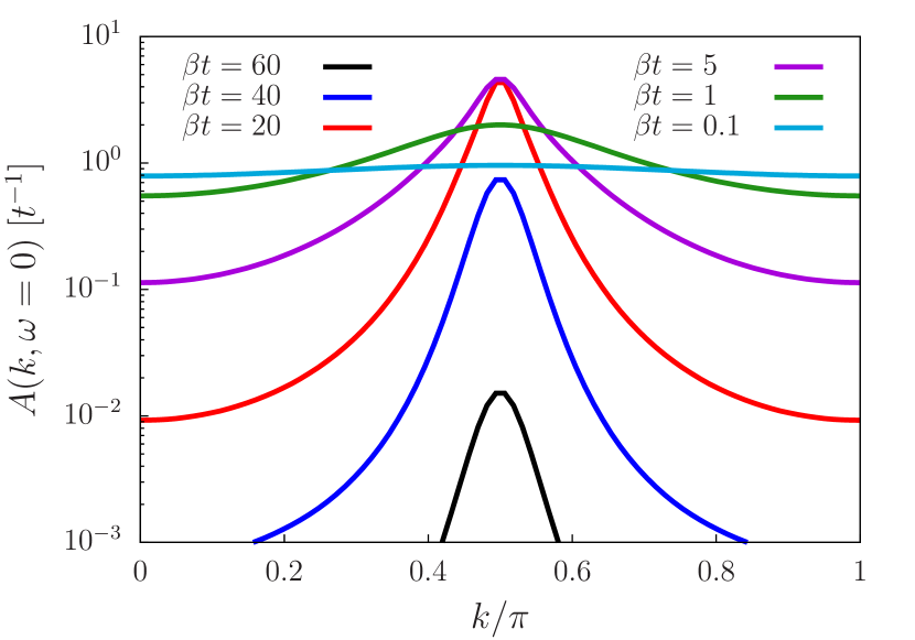
Figure 9: (Color online) Temperature dependence of the zero-energy peak in $A(k,\omega)$ as a function of momentum $k$ for the SSH model for $\lambda=0.75$ and $L=162$. The spectrum was averaged over an interval $\Delta\omega=0.04t$ around $\omega=0$. Hence, the extent of the peak in frequency is not captured.

We attribute the zero-energy mode in the single-particle spectrum to soliton states at thermally generated domain walls between different lattice dimerizations [11; 30]. We can estimate the spatial extent of these states from their momentum dependence, which is shown in Fig. 9. At low temperatures, the shape of the peak hardly changes, only its spectral weight becomes larger. A comparison with the analytic result for the soliton wave function [30], $\phi_{0}(n)\sim\mathrm{sech}(n/l)\cos(\pi n/2)$, gives a localization length of $l\approx 5$ in units of the lattice spacing, in agreement with Ref. [30]. As the temperature exceeds $\beta t=20$, the peak in Fig. 9 broadens in $k$-space and the localization length becomes smaller. In the high-temperature limit, the zero-energy state becomes completely localized. Although the picture of domain walls between ordered regions breaks down when the single-particle gap closes, the zero mode persists at higher temperatures [Fig. 8(d)] where it can be understood as a disorder effect, see Sec. V.3.

V.2.4 Optical conductivity

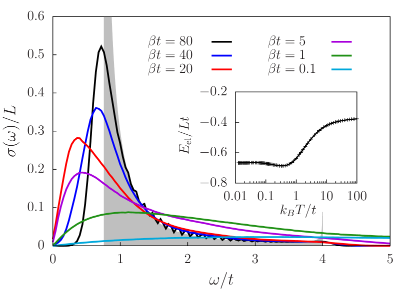
Figure 10: (Color online) Optical conductivity of the SSH model for $\lambda=0.75$ and $L=162$. The filled curve is the $T=0$ mean-field result (20). The inset shows the energy of the electronic subsystem as a function of temperature. It is related to $\sigma(\omega)$ by the sum rule given in Eq. (21).

The optical conductivity $\sigma(\omega)$ is shown in Fig. 10. At $T=0$, the mean-field result is given by

$$\sigma(\omega)=\frac{4L\Delta^{2}t^{2}}{\pi\omega^{2}}\frac{1}{\sqrt{\omega^{2}-\Delta^{2}}}\frac{1}{\sqrt{(4t)^{2}-\omega^{2}}}$$ (20)

for $\Delta<\left|\omega\right|<4t$, otherwise it is zero. Compared to the Holstein model, it has an additional square-root singularity at the upper edge of the spectrum. However, its integrated weight is too small to be visible even at the lowest temperature considered. The lower edge first broadens and then also shifts to lower frequencies. Similar to the Holstein model, up to $\beta t\approx 10$ spectral weight is only redistributed, as visible from the inset of Fig. 10. The integrated spectrum is related to the energy of the electronic subsystem via the sum rule [53]

$$\int_{0}^{\infty}d\omega\,\sigma(\omega)=-\frac{\pi}{2}E_{\mathrm{el}}\,.$$ (21)

In contrast to the Holstein model, the sum rule also includes the interaction energy of electrons and phonons. Because of this contribution, the integrated weight slightly increases between $\beta t\approx 10$ and $\beta t\approx 3$. Further increasing the temperature leads to a reduction of spectral weight at small $\omega$ and a substantial enhancement of the tail at large $\omega$. In contrast to the Holstein model, the integrated weight does not vanish for $T\to\infty$.

V.3 Relation to disorder problems

At high temperatures, the essentially random lattice distortions act as disorder for the electrons [29], corresponding to site disorder for the Holstein model, and bond disorder for the SSH model. The probability distribution $W[C]$ [Eq. (8)] becomes a Gaussian and the disorder strength scales as $\sqrt{\lambda T}$. The connection to disordered noninteracting models explains some of the spectral features observed above.

For the Holstein model, the strong onsite disorder leads to two distinct peaks in the two-particle spectra [Figs. 4(h) and 6], one at $\omega=0$ in $S_{\rho}(q,\omega)$, and another at $\omega=2t$ both in $S_{\rho}(q,\omega)$ and $\sigma(\omega)$. The zero-energy peak in $S_{\rho}(q,\omega)$ does not show any $q$ dependence, whereas the peak at $\omega=2t$ is strongest around $q=\pi$, but vanishes at $q=0$. The latter signature also appears in $\sigma(\omega)$, where it has already been observed for the $t-V$ model at strong disorder [54] and the Holstein polaron in the adiabatic regime [55]. This signature becomes even sharper as temperature is increased further. In Ref. [55], the resonance at $\omega=2t$ has been explained from an effective two-site model, where the bonding and antibonding eigenstates of the electron perfectly overlap with the current operator. In the same way, $\hat{n}_{q}$ connects the different-parity states at $q=\pi$, whereas the overlap is zero at $q=0$.

For the SSH model, only the zero-energy peak appears in the high-temperature limit of $S_{b}(q,\omega)$. Moreover, an excitation with $\omega=0$ is visible in the single-particle spectrum and persists for $T\to\infty$. Such a peak has previously been observed for the SSH polaron [41] and explained as a disorder effect [56; 57; 58; 59]. For the tight-binding model, any finite off-diagonal disorder leads to a zero-energy peak in the density of states that becomes larger and broadens as the disorder strength increases [57]. The appearance of the peak is related to the chiral symmetry of the SSH Hamiltonian. The latter is broken by onsite disorder, and the zero mode disappears accordingly [57]. Moreover, no zero mode exists for the Holstein model for which chiral symmetry is broken already at the mean-field level. While we have so far interpreted the zero-energy excitations at low temperatures in terms of topologically protected soliton states located at domain walls, such states can also be induced by off-diagonal disorder acting on the dimerized ground state [60; 61; 62; 63].

At low temperatures, the broadening of the spectral functions can be considered as a disorder effect, including the tail of the optical conductivity extending into the mean-field gap. For the Holstein model, it is related to the weak pinning of a charge-density wave by onsite disorder [64]. For the SSH model, similar results were also obtained from the fluctuating gap model, where order parameter fluctuations are modeled as off-diagonal disorder [65; 62; 63; 66; 67].

VI Conclusions

We presented exact numerical results for the thermodynamic and spectral properties of Peierls insulators within the framework of spinless Holstein and SSH models in the adiabatic limit. In this limit, a dimerized Peierls state with long-range charge and lattice order exists for any nonzero electron-phonon coupling at zero temperature, as described by mean-field theory. Using a Monte Carlo method to sample the classical phonons, we investigated the impact of thermal fluctuations on the specific heat, the single-particle spectrum, the dynamic density and bond structure factors, as well as the optical conductivity. In contrast to the quantum case, we were able to calculate spectra without using analytic continuation.

Thermal fluctuations destroy the mean-field long-range order, and give rise to a characteristic low-temperature peak in the specific heat. While there is no finite-temperature phase transition in the 1D case considered, the peak occurs at the temperature scale at which the Peierls gap is filled in by thermal fluctuations. A similar peak has previously been observed in theory and experiment. Thermally excited solitons manifest themselves as in-gap excitations. In the Holstein model, the latter appear symmetrically around the Fermi level only at low temperatures, whereas in the SSH model they are pinned to zero energy and persist for all temperatures due to the chiral symmetry of the Hamiltonian. The filling of the Peierls gap by thermal excitations is also reflected in the two-particle excitation spectra and the optical conductivity. For the latter, we observe a nontrivial interplay of enhanced low-frequency transport due to a thermally reduced Peierls gap and a suppression due to the onset of incoherence. Finally, at high temperatures, the spectral features of the electron-phonon models are related to those of models with site or bond disorder.

The results obtained here in the adiabatic limit provide exact benchmarks. In contrast to the widely used mean-field approximation, all thermal fluctuations (i.e., amplitude fluctuations of the order parameter and solitons) are taken into account and finite-size effects are negligible at all but the lowest temperatures. Our findings at low temperatures complement previous work on the case with quantum phonons. In particular, the spectral functions reveal many of the characteristic features observed for quantum Holstein and SSH models [40; 13]. The adiabatic approximation is expected to quantitatively capture the physics of the quantum case for temperatures large compared to the Peierls gap. Finally, the present findings provide a platform for the thermodynamics of quantum phonon models, for which finite-size effects and uncertainties related to the analytic continuation pose significant challenges to simulations.

*

Appendix A Finite-size analysis of the specific heat

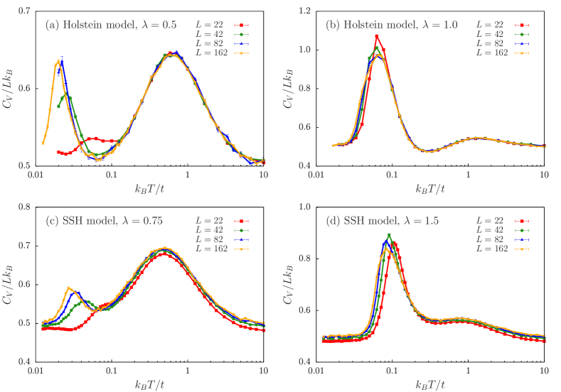
Figure 11: (Color online) Specific heat of the Holstein model [(a), (b)] and the SSH model [(c), (d)] for different system sizes $L$.

In Sec. IV we discussed the low-temperature behavior of $C_{V}$, and observed the appearance of a peak related to the ordering of the lattice. A reliable analysis also requires a study of finite-size effects. Therefore, we present in Fig. 11 $C_{V}$ as a function of temperature for different system sizes ranging from $L=22$ to $L=162$, and for two values of the electron-phonon coupling.

Figure 11(a) shows data for the Holstein model with $\lambda=0.5$. For temperatures $k_{\text{B}}T>0.1t$, $C_{V}$ has already converged at the smallest $L$ considered, whereas for lower temperatures a clear dependence on the lattice size is visible. Between $L=22$ and $L=82$, both the position of the low-temperature peak and its height change substantially. The upturn to its maximum is only converged for the two largest lattice sizes. At $\lambda=1$ [Fig. 11(b)], the peak appears at higher temperatures and its upturn is already converged for $L=22$. While the height of the maximum has converged for $L=82$, the subsequent downturn to the lowest temperatures measured still changes from $L=82$ to $L=162$. Note that error bars are large in this temperature regime and adjacent data points are not independent due to the use of parallel tempering.

For the SSH model, finite-size effects on $C_{V}$ are also visible at high temperatures [Fig. 11(c) and 11(d)]. However, these effects are simply related to the fact that only $L-1$ phonon modes contribute to $C_{V}$ because the length of the chain is fixed and the $k=0$ mode drops out of the Hamiltonian. The finite-size effects at low temperatures are slightly larger than for the Holstein model. For $\lambda=0.75$ [Fig. 11(c)], the peak position and height still change up to $L=162$. Compared to the finite-size convergence in the Holstein model at $\lambda=0.5$ [Fig. 11(a)], we believe that the upturn at $L=162$ is converged. For $\lambda=1.5$ [Fig. 11(d)] it is indeed converged, but the subsequent downturn again shows finite-size effects.

The above analysis suggests that except for the downturn at the lowest temperatures considered, the $C_{V}$ data shown in Fig. 1 have converged with respect to $L$. The finite-size effects on $C_{V}$ may also be consulted in order to estimate finite-size effects on the spectral functions.

References

- Claessen et al. [2002] R. Claessen, M. Sing, U. Schwingenschlögl, P. Blaha, M. Dressel, and C. S. Jacobsen, Phys. Rev. Lett. 88, 096402 (2002).
- Travaglini et al. [1983] G. Travaglini, I. Mörke, and P. Wachter, Solid State Commun. 45, 289 (1983).
- Voit [1995] J. Voit, Rep. Prog. Phy. 57, 977 (1995).
- Yonemitsu and Nasu [2008] K. Yonemitsu and K. Nasu, Phys. Rep. 465, 1 (2008).
- Fröhlich [1954] H. Fröhlich, Proc. Roy. Soc. A 223, 296 (1954).
- Peierls [1955] R. E. Peierls, Quantum Theory of Solids (Clarendon, Oxford, 1955).
- Heeger et al. [1988] A. J. Heeger, S. Kivelson, J. R. Schrieffer, and W. P. Su, Rev. Mod. Phys. 60, 781 (1988).
- Grüner [1988] G. Grüner, Rev. Mod. Phys. 60, 1129 (1988).
- Pouget [2016] J.-P. Pouget, Comptes Rendus Physique 17, 332 (2016).
- Holstein [1959] T. Holstein, Ann. Phys. (N.Y.) 8, 325 (1959); 8, 343 (1959).
- Su et al. [1979] W. P. Su, J. R. Schrieffer, and A. J. Heeger, Phys. Rev. Lett. 42, 1698 (1979).
- Hohenadler and Assaad [2013] M. Hohenadler and F. F. Assaad, Phys. Rev. B 87, 075149 (2013).
- Weber et al. [2015] M. Weber, F. F. Assaad, and M. Hohenadler, Phys. Rev. B 91, 245147 (2015).
- Fradkin and Hirsch [1983] E. Fradkin and J. E. Hirsch, Phys. Rev. B 27, 1680 (1983).
- Jeckelmann et al. [1999] E. Jeckelmann, C. Zhang, and S. R. White, Phys. Rev. B 60, 7950 (1999).
- Schmeltzer et al. [1986] D. Schmeltzer, R. Zeyher, and W. Hanke, Phys. Rev. B 33, 5141 (1986).
- Nakahara and Maki [1982] M. Nakahara and K. Maki, Phys. Rev. B 25, 7789 (1982).
- Greitemann et al. [2015] J. Greitemann, S. Hesselmann, S. Wessel, F. F. Assaad, and M. Hohenadler, Phys. Rev. B 92, 245132 (2015).
- Craven et al. [1974] R. A. Craven, M. B. Salamon, G. DePasquali, R. M. Herman, G. Stucky, and A. Schultz, Phys. Rev. Lett. 32, 769 (1974).
- Wei et al. [1977] T. Wei, A. Heeger, M. Salamon, and G. Delker, Solid State Commun. 21, 595 (1977).
- Huizinga et al. [1979] S. Huizinga, J. Kommandeur, G. A. Sawatzky, B. T. Thole, K. Kopinga, W. J. M. de Jonge, and J. Roos, Phys. Rev. B 19, 4723 (1979).
- Dardel et al. [1992] B. Dardel, D. Malterre, M. Grioni, P. Weibel, Y. Baer, C. Schlenker, and Y. Pétroff, Europhys. Lett. 19, 525 (1992).
- Mou et al. [2014] D. Mou, R. M. Konik, A. M. Tsvelik, I. Zaliznyak, and X. Zhou, Phys. Rev. B 89, 201116 (2014).
- Louis et al. [2006] K. Louis, P. Prelovšek, and X. Zotos, Phys. Rev. B 74, 235118 (2006).
- Kühne and Löw [1999] R. W. Kühne and U. Löw, Phys. Rev. B 60, 12125 (1999).
- Bühler et al. [2004] A. Bühler, G. S. Uhrig, and J. Oitmaa, Phys. Rev. B 70, 214429 (2004).
- Michielsen and de Raedt [1996] K. Michielsen and H. de Raedt, Mod. Phys. Lett. B 10, 467 (1996).
- Michielsen and De Raedt [1997] K. Michielsen and H. De Raedt, Zeitschrift für Physik B Condensed Matter 103, 391 (1997).
- Brazovskii and Dzyaloshinskii [1976] S. A. Brazovskii and I. E. Dzyaloshinskii, Zh. Eksp. Teor. Fiz. 71, 2338 (1976).
- Su et al. [1980] W. P. Su, J. R. Schrieffer, and A. J. Heeger, Phys. Rev. B 22, 2099 (1980).
- Hirsch and Fradkin [1983] J. E. Hirsch and E. Fradkin, Phys. Rev. B 27, 4302 (1983).
- Lee et al. [1974] P. Lee, T. Rice, and P. Anderson, Solid State Commun. 14, 703 (1974).
- Mermin and Wagner [1966] N. D. Mermin and H. Wagner, Phys. Rev. Lett. 17, 1133 (1966).
- Ryu and Hatsugai [2002] S. Ryu and Y. Hatsugai, Phys. Rev. Lett. 89, 077002 (2002).
- Asbóth et al. [2016] J. K. Asbóth, L. Oroszlány, and A. Pályi, A Short Course on Topological Insulators, Lecture Notes in Physics, Vol. 919 (Springer, 2016).
- Schnyder et al. [2008] A. P. Schnyder, S. Ryu, A. Furusaki, and A. W. W. Ludwig, Phys. Rev. B 78, 195125 (2008).
- Kitaev [2009] A. Kitaev, AIP Conf. Proc. 1134, 22 (2009).
- Ryu et al. [2010] S. Ryu, A. P. Schnyder, A. Furusaki, and A. W. W. Ludwig, New Journal of Physics 12, 065010 (2010).
- Jackiw and Rebbi [1976] R. Jackiw and C. Rebbi, Phys. Rev. D 13, 3398 (1976).
- Hohenadler et al. [2011] M. Hohenadler, H. Fehske, and F. F. Assaad, Phys. Rev. B 83, 115105 (2011).
- Cataudella et al. [2011] V. Cataudella, G. De Filippis, and C. A. Perroni, Phys. Rev. B 83, 165203 (2011).
- Metropolis et al. [1953] N. Metropolis, A. W. Rosenbluth, M. N. Rosenbluth, A. H. Teller, and E. Teller, J. Chem. Phys. 21, 1087 (1953).
- Anderson [1958] P. W. Anderson, Phys. Rev. 109, 1492 (1958).
- Onishi and Miyashita [2000] H. Onishi and S. Miyashita, J. Phys. Soc. Jpn. 69, 2634 (2000).
- Hukushima and Nemoto [1996] K. Hukushima and K. Nemoto, J. Phys. Soc. Jpn. 65, 1604 (1996).
- Schulz [1987] H. J. Schulz, “The crossover from one to three dimensions: Peierls and spin-peierls instabilities,” in Low-Dimensional Conductors and Superconductors, edited by D. Jérome and L. G. Caron (Springer US, Boston, MA, 1987) pp. 95–112.
- Scalapino et al. [1972] D. J. Scalapino, M. Sears, and R. A. Ferrell, Phys. Rev. B 6, 3409 (1972).
- Landau [1937] L. D. Landau, Zh. Eksp. Teor. Fiz. 7, 19 (1937).
- Jérome and Schulz [1982] D. Jérome and H. J. Schulz, Adv. Phys. 31, 299 (1982).
- Kadanoff and Baym [1989] L. P. Kadanoff and G. A. Baym, Quantum Statistical Mechanics: Green’s Function Methods in Equilibrium and Nonequilibrium Problems (Addison-Wesley, Redwood City, California, 1989).
- Lee et al. [1973] P. A. Lee, T. M. Rice, and P. W. Anderson, Phys. Rev. Lett. 31, 462 (1973).
- Voit et al. [2000] J. Voit, L. Perfetti, F. Zwick, H. Berger, G. Margaritondo, G. Grüner, H. Höchst, and M. Grioni, Science 290, 501 (2000).
- Capone et al. [1997] M. Capone, W. Stephan, and M. Grilli, Phys. Rev. B 56, 4484 (1997).
- Barišić and Prelovšek [2010] O. S. Barišić and P. Prelovšek, Phys. Rev. B 82, 161106 (2010).
- Schubert et al. [2005] G. Schubert, G. Wellein, A. Weisse, A. Alvermann, and H. Fehske, Phys. Rev. B 72, 104304 (2005).
- Dyson [1953] F. J. Dyson, Phys. Rev. 92, 1331 (1953).
- Theodorou and Cohen [1976] G. Theodorou and M. H. Cohen, Phys. Rev. B 13, 4597 (1976).
- Soukoulis and Economou [1981] C. M. Soukoulis and E. N. Economou, Phys. Rev. B 24, 5698 (1981).
- Fleishman and Licciardello [1977] L. Fleishman and D. C. Licciardello, J. Phys. C: Solid State Phys. 10, L125 (1977).
- Mostovoy et al. [1997] M. V. Mostovoy, M. T. Figge, and J. Knoester, Europhys. Lett. 38, 687 (1997).
- Bartosch and Kopietz [1999a] L. Bartosch and P. Kopietz, Phys. Rev. Lett. 82, 988 (1999a).
- Bartosch and Kopietz [1999b] L. Bartosch and P. Kopietz, Phys. Rev. B 60, 15488 (1999b).
- Millis and Monien [2000] A. J. Millis and H. Monien, Phys. Rev. B 61, 12496 (2000).
- Fukuyama and Lee [1978] H. Fukuyama and P. A. Lee, Phys. Rev. B 17, 535 (1978).
- Kim et al. [1993] K. Kim, R. H. McKenzie, and J. W. Wilkins, Phys. Rev. Lett. 71, 4015 (1993).
- Monien [2001] H. Monien, Phys. Rev. Lett. 87, 126402 (2001).
- Bartosch [2004] L. Bartosch, Europhys. Lett. 65, 68 (2004).
- Jülich Supercomputing Centre [2016] Jülich Supercomputing Centre, Journal of large-scale research facilities 2, A62 (2016).