Identification of refugee influx patterns in Greece via model-theoretic analysis of daily arrivals

Abstract

The refugee crisis is perhaps the single most challenging problem for Europe today. Hundreds of thousands of people have already traveled across dangerous sea passages from Turkish shores to Greek islands, resulting in thousands of dead and missing, despite the best rescue efforts from both sides. One of the main reasons is the total lack of any early warning/alerting system, which could provide some preparation time for the prompt and effective deployment of resources at the “hot” zones. This work is such an attempt, the first completely data-driven study for a systemic analysis of the refugee influx in Greece, aiming at: (a) the statistical and signal-level characterization of the smuggling networks and (b) the formulation and preliminary assessment of such models for predictive purposes, i.e., as the basis of such an early warning/alerting protocol. To our knowledge, this is the first-ever attempt to design such a system, since this refugee crisis itself and its geographical properties are unique (intense event handling, little/no warning). The analysis employs a wide range of statistical, signal-based and matrix factorization (decomposition) techniques, including linear & linear-cosine regression, spectral analysis, ARMA, SVD, Probabilistic PCA, ICA, K-SVD for Dictionary Learning, as well as fractal dimension analysis. It is established that the behavioral patterns of the smuggling networks closely match (as expected) the regular “burst” and “pause” periods of store-and-forward networks in digital communications. There are also major periodic trends in the range of 6.2-6.5 days and strong correlations in lags of four or more days, with distinct preference in the Sunday/Monday 48-hour time frame. These results show that such models can be used successfully for short-term forecasting of the influx intensity, producing an invaluable operational asset for planners, decision-makers and first-responders.

I Introduction

Since early January 2015, Europe has witnessed an unprecedented influx of refugees from regions of war and conflict in the Middle East, primarily Syria, Afghanistan and Iraq. For more than 17 months now, Greece has become the main entrance gateway for hundreds of thousands of people trying to get to central and northern European countries. According to the United Nations High Commissioner for Refugees (UNHCR) [1], the International Organization for Migration (IOM) [2] and the Medecins Sans Frontieres (MSF) [3], during the year 2015 alone, more than a million people reached Europe from Turkey and North Africa, seeking safety and asylum.

In this context, the rapid allocation of proper resources is the most critical factor in the success or failure of any rescue and relief operations, especially in the “hot” zones. On the other hand, the complete coverage of these areas of interest by patrols alone is practically infeasible due the geographical extent of possible landing points, as well as the excessive financial cost if these operations are to be maintained on 24-hour rotation for many weeks and months. Therefore, an early warning/alerting system for (expected) high refugee influx, analogous to the ones used for extreme weather conditions or possible wildfires in forests, would provide invaluable time for the preparation and deployment of teams and equipment from staging posts to specific areas of interest, promptly and effectively, in order to save lives.

This study is the first (to our best knowledge) attempt for a completely data-driven systemic analysis of the refugee influx data series, aiming at: (a) the statistical and signal-level characterization of the smuggling networks as a generating process; and (b) the draft formulation and preliminary assessment of such models for predictive purposes, i.e., to produce short-term forecasting of the refugee influx, as part of an early warning/alerting protocol. After the description of the material (data series) used, a wide range of statistical, signal-based, spectral and component analysis (decomposition) techniques are presented in brief, each accompanied with the corresponding results and the conclusions drawn from them. Finally, the general findings are further discussed and future enhancements are proposed.

I-A Background

There are only few passages across the sea borders between Greece and Turkey where the distance is 5-7.5 n.m., hence these are the points of interest for both the smuggling networks and the coast guard patrols. At least 856,723 people came to Greece via Turkey, 80% of which landed at the island of Lesvos in the northern Aegean Sea. Nevertheless, the lack of proper infrastructure, first-response coordination, early warning and on-the-spot logistical support resulted in thousands of casualties. The seer volume of the influx resulted in a total of 3,771 registered dead or missing persons in the Mediterranean Sea during 2015 [4, 1] , more than 832 in the Aegean Sea. There were specific 24-hour time frames at the end of October and the beginning of November 2015 when small beaches in the northern shores of Lesvos, like the small port of Skala Sykamneas with a population of only a few hundreds, received over 120 boats landing there, each carrying 40-50 persons.

During 2015, the Hellenic Coast Guard (HCG) has conducted over 6,300 Sea Search & Rescue (SSAR) operations in these areas and more than 117,743 people have been rescued in the Aegean Sea [5]; additionally, Turkish Coast Guard (TCG) has rescued at least 59,377 people, plus 339 dead or missing, in other incidents [6]. Therefore, it is estimated that roughly 177,120 in 856,723 or more than one in five people (1:4.84) coming across these passages ended up rescued from the water; adding up the (estimated) dead and missing [2], at least 832 in 177,952 or 1:214 (about two persons every nine boats that sank) ended up dead or missing somewhere in the Aegean Sea.

The first quarter of 2016 up the the first weeks of April resulted in just over 178,882 arrivals in the Mediterranean Sea and another 737 dead or missing [2]. More specifically, there are 356 deaths in 24,581 arrivals in Italy and 375 deaths in 153,625 arrivals in Greece, the two major entrance points to Europe via the Central/Eastern Med. routes (update: April 19th, 2016 [7]). This yields a death ratio of 1:69 for Italy but 1:410 for Greece, i.e., almost six times deadlier in comparison.

It should also be noted that the deaths from sinking of migrant/refugee ships inbound to Italy are usually underestimated due to the difficulties in locating all the bodies in the open sea, as well as the under-reporting of passengers on board. On April 18th 2016, a 30m boat capsized during the night between Libya and Sicily, carrying an estimated 500-550 people; only 41 were rescued and a few dozen bodies were recovered by the Italian Coast Guard (ICG) [8]. Similar major events have occurred in the past, on October 3rd & 11th 2013 (394+ dead/missing) and on April 20th 2014 (800 dead/missing), with survival rates of less than 28% [9, 10].

Operation Mare Nostrum was a year-long naval and air mission involving the Italian Coast Guard and Navy, after the major shipwrecks of October 2013 in the Central Med. route from North Africa [11]. During this period, more than 150,000 migrants and refugees were successfully rescued in the sea. The operation ended in October 31st 2014 and it was superseded by EU Frontex’s Operation Triton [12], another border patrol & SSAR mission, with a much smaller force (on a volunteer basis by 15 other European countries) and a much more limited range in the same area. As a result, the incidents with hundreds of people missing in the sea and the survival rates returned to their prior states.

Despite the dreadful probabilities, migrants and refugees still prefer to make their attempt via sea to Greece or Italy rather than via land (mostly Turkish-Bulgarian borders) by a rate of more than 42:1, because sea borders are inherently harder to patrol, fence or deny rescue. This is a very clear explanation of why these narrow sea crosses between Turkish sail-off beaches and the Greek islands received such a huge volume of refugee influx, sometimes 5,000 people or more on a daily basis, e.g. 12,000+ people within the 48 hours of 27-28 October 2015. Figure 1 and Figure 2 illustrate how this looks like in real life, with snapshots taken on October 2015 (photo) and February 2016 (map).

Figure 1: A snapshot photograph from the northern beaches of Lesvos on October 2015, showing nine inflatable boats carrying 40-50 each, heading to the landing zone with only minutes apart (Credit: AFP / Aris Messinis).

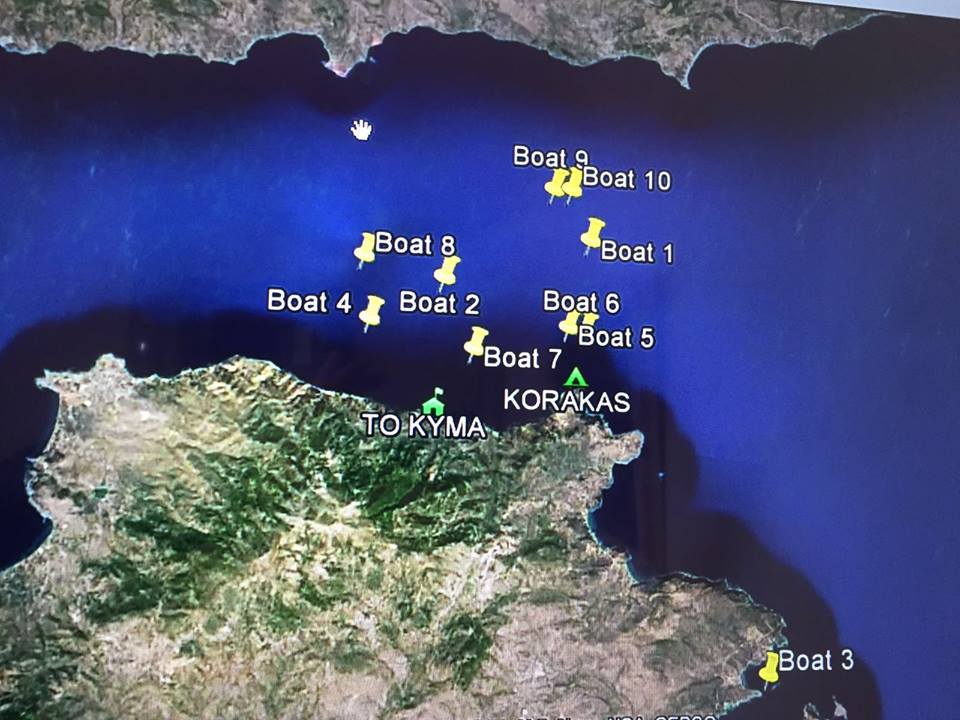
Figure 2: A snapshot from a live Google map used by the SSAR elements in northern Lesvos, showing the identified refugee boats heading towards the island on February 17th, 2016 (13:37’ local) (Credit: Proactiva Open Arms).

After the recent EU-Turkey deal in March 2016 [13], regarding the handling of asylum seekers and their mutual transfer after proper registration, the influx to the EU is starting to shift again from the Eastern (Greece) to the Central (Italy) Med. sea route, resulting in a sharp rise of dead and missing ratios in boat sinking incidents.

According to more recent numbers from IOM and MSF, by early May about 1,200 people have died in the Mediterranean Sea trying to reach Europe. MSF, who has recently resumed its own SSAR operations in the area between Libya and Italy, estimate that 976 people have died trying to cross from Libya to Europe so far this year (early May), yielding a death ratio of roughly 1:30. The boat trip from Libya to Italy is much longer and perilous than the crossings from Turkey to Greece, 8-12 hours for about 150 n.m. rather than 25-40 minutes for 5-7.5 n.m. in comparison. As a result, massive boat sinking and capsizing events every week are drastically increasing the death/missing total and the true death ratio in the Central Med. route to Europe.

I-B Problem statement

The most challenging task in managing such intense influx of refugees in the very large coastline of Greece, in such a short notice due to the very short distance from Turkey, is being the proper allocation and rapid response of SSAR resources, as well as medical care at the beaches and ports in case of shipwrecks. Unfortunately, neither the resources nor the coordination was in place when it was needed the most. Figure 3 shows the total refugee influx intensity in all the Greek islands during 2015 and the first months of 2016 [4], peaking around the period September-November 2015. During that time frame, at least half of the rescues were conducted by volunteers, fishermen and other non-tasked vessels, while first-response medical care was often performed on the ground with little to no resources available to extremely limited staff (primarily volunteer doctors and lifeguards).

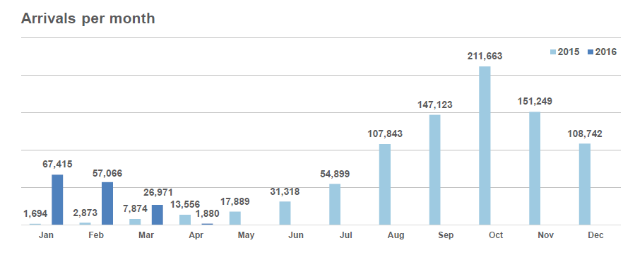
Figure 3: Refugee influx statistics per month, 2015 and early 2016 (Greece).

In this specific context, there were two additional factors that made rapid response an imperative necessity. First, the winter season, with rough sea condition and low temperatures, shrinking the survival time in case of shipwrecks, since people did not have any protective gear (thermal suits) other than life vests, if any. Second, as Figure 4 shows, the demographics of the refugees arriving during the second half of 2015 shifted from primarily men (73%, June 2015) to primarily women and children (57%, Jan. 2016) [4]. This means that the physical endurance and the average survival time of people involved in shipwrecks were becoming inherently worse, despite of weather conditions.

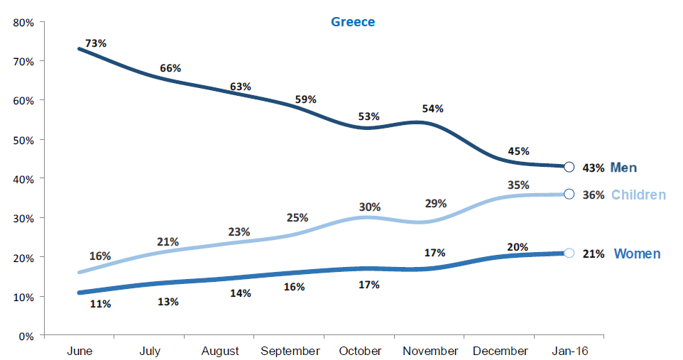
Figure 4: Refugee population demographics, mid-2015 and early 2016 (Greece).

It is clear that, despite any efforts to find solutions in the political level for the refugee crisis at hand, the problems on the ground require well-informed decisions, high mobility and rapid response, in order to save lives. The primary concern for the SSAR resources, the medical teams, the volunteers and the NGOs assisting in the humanitarian relief, as well as the proper logistics and warehouse management in the first-reception islands, are all centered around the influx of refugees via unsafe boats. The problem is inherently one of humanitarian crisis management; on the other hand, the major difficulty is not the lack of civil infrastructure (e.g. electricity, open roads, communications, etc) as in a large earthquake or a flood, but rather in the ability to allocate adequate resources rapidly in various spots. Therefore, one of the most important and challenging tasks for a successful operation in this context is to enlarge the time frame for short-term planning deployment, i.e., improve the capabilities of early warning & prompt alerting. It is a concept that is already included in emergency planning and emergency operations in other contexts, for example in forecasting water levels to issue early warnings for possible floods, assessing weather conditions (humidity, temperature) to issue alert warnings for possible wildfires in forests, etc.

This study is an attempt to quantify and analyze in a systemic way the task of developing such early warning/alert systems in the context of refugee influx, using Greece and the Aegean Sea islands as the main paradigm. To our knowledge, this is the first-ever attempt to design such a system, since this refugee crisis itself and its geographical properties is unique in its own way. The goal is to identify the underlying statistical properties and the inherent “system” that produces this influx, without any prior knowledge or insight of how the smuggling networks operate near the Turkish coasts. Based on reliable data, these models can then be used as guidelines for short-term forecasting of the influx intensity, hence produce an invaluable operational asset for planners, decision-makers and first-responders.

II Material and Data Overview

II-A Daily arrivals data series

This study is based on official data provided by UNHCR sources for the daily arrivals of refugees in the Greek islands of the eastern Aegean Sea [14, 15, 1]. Specifically, UNHCR provides detailed daily logs of people registered in the “hotspot” camps in the islands, as well as from verified sources (other NGOs, Hellenic Coast Guard, Frontex). The reason for having “estimated” and not exact numbers is that new arrivals may not be registered immediately or UNHCR may not get informed promptly by the other actors. The result of this data collection process is a mashup of data for the daily arrivals in each one of the main reception islands, a grand total for Greece and a series of explanatory reports.

Figure 5: Estimated daily arrivals and weekly averages for the entire Greece (Oct.2015-Jan.2016).

There are six main regions of interest in the Aegean Sea: the islands of Lesvos, Chios, Samos, Leros, Kos and the rest of the southern Dodecanese islands. Figure 5 illustrates the main data series for the composite total of daily arrivals in the entire Aegean Sea, while Figure 6 illustrates the individual daily arrivals in each of the six regions of interest.

Figure 6: Estimated daily arrivals and weekly averages for the six main regions of interest in the Aegean Sea.

In this study only the main data series was used for the analysis, since more than 80% of the influx is related mostly to Lesvos and Chios. Furthermore, using the grand total of influx is inherently more robust in terms of canceling individual noisy factors and enabling the identification of global statistical trends. The time frame used in this case for the data series is from 1-Oct-2015 to 16-Jan-2016, a total span of 108 consecutive days (almost 15 weeks). The entire data series is used in several analysis methods below, while a weekly-grouped version of a slightly truncated data series in “matrix” mode (15x7 = 105 days) is used by other methods, as described in each case later on.

II-B Software packages and hardware

The main software packages that were used in this study were:

• Mathworks MATLAB v8.6 (R2015b), including: Signal Processing Toolbox, System Identification Toolbox, Statistics & Machine Learning Toolbox [16].

• Additional toolboxes for MATLAB (own & third-party) for specific algorithms, as referenced later on in the corresponding sections.

• WEKA v3.7.13 (x64). Open-Source Machine Learning Suite [17].

• Spreadsheet applications: Microsoft Excel 2007, LibreOffice Sheet 5.1 (x64).

• Custom-built programming tools in Java and C/C++ for data manipulation (import/export).

The data experiments and processing were conducted using: (a) Intel i7 quad-core @ 2.0 GHz / 8 GB RAM / MS-Windows 8.1 (x64), and (b) Intel Atom N270 dual-core @ 1.6 GHz / 2 GB RAM / Ubuntu Linux 14.04 LTS (x32).

III Basic statistics

The standard histogram plot of the signal can provide the basic statistical properties of the data when no time dependency (sequencing) is taken into account. Figure 7 illustrates the distribution of the daily arrivals (volume) for six bins, while Table I contains the range statistics and the first moments of the data [18, 19, 20].

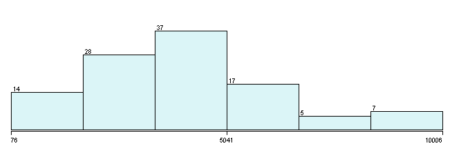
Figure 7: Histogram plot of the daily arrivals (108 points).

TABLE I: Basic statistics of the daily arrivals (108 points).

Parameter	Value
minimum	76
maximum	10,006
median	4,077
mean	4,151.51
stdev	2,216.79
skewness	0.497
kurtosis	0.081

From the histogram in Figure 7, it is evident that the left and the right section of the Gaussian-like distribution around the mean are somewhat different, with the first (lower values) being “thicker” than the standard deviation and the second (higher values) being “thinner” but more widely spread in terms of maximum range. This means that the values below the average daily arrivals are somewhat more common, but the values above the average spread to a higher range. In practice, the high influx rates in daily arrivals are somewhat fewer, with larger absolute deviation against the mean, compared to the corresponding low influx rates that are a bit more common, with smaller deviation against the mean. This observation is consistent with the daily reports from the people involved in the actual registration process in the landing areas.

In terms of statistics, these asymmetries are quantified by the kurtosis parameter, which describes the “sharpness” of the central Gaussian-like lobe of the histogram, and the skewness parameter, which describes the asymmetry of the lobe against the mean value (for Normal distribution, both kurtosis and skewness are zero). Here, kurtosis value is close to zero, but the large positive value of skewness translates to a “heavy right tail” in the corresponding distribution – roughly 11.1% of the daily arrivals are above 6,700. This asymmetry is also encoded by the clear difference between the median and the mean values, where the second is larger (to the “right”) but both below the absolute middle of the value range, i.e., min+(max-min)/2=5,041.

One more important note is related to the value of standard deviation $\left(\sigma\right)$: In any statistical distribution that can be modeled effectively by Gaussian-like approximation, the range $\left[-\sigma\ldots+\sigma\right]$ contains roughly 68% and $\left[-2\sigma\ldots+2\sigma\right]$ contains roughly 95% of the data [18, 19]. This general observation is very important for translating the standard deviation into a usable predictive factor, since in this case it means that at least 2/3 of the daily arrivals are in the approximate range of $\mu=4,151\pm 2,217$. However, daily arrivals is a time series, i.e., the data have specific time structuring (sequencing) and therefore general predictive analytics, such as confidence ranges for the mean value, are less important here compared to other auto-regressive and decomposition approaches that are described later on.

For completeness, the histogram in Figure 7 was approximated by best-fit Poisson and Generalized Extreme Value (GEV) [21] distributions. The data series is clearly a zero-bounded set, compatible to the GEV formulation, and it corresponds to “events” or “arrivals”, compatible to the Poisson formulation. The best-fit parameters of the distributions in both cases were calculated by Maximum Likelihood Estimation (MLE) for significance level 95% $\left(\alpha=0.05\right)$. For Poisson, parameter lambda is $\lambda=4,151.5\pm 12.5$, which is identical to the Gaussian mean value. For GEV, parameters are shape $\xi=-0.15\pm 0.15$, scale $\sigma=1,980\pm 297$ and location $\mu=3,240\pm 419$, which makes it narrower than the Gaussian distribution and shifted to the left, i.e., towards the lower bound (zero), as expected.

Figure 8 illustrates the daily arrivals grouped by week, starting from day 4 to day 108, producing 15x7 or 105 days in total, i.e., excluding the first three days of the original data series. Cells are colored according to their relative influx intensity, from low (blue) to high (red) and intermediate values (green/cyan). The horizontal axis represents weekdays (Monday=1, Sunday=7) and the vertical axis represents elapsed weeks from the start. Figure 9 shows the corresponding weekday averages, taken against the columns of the “matrix” illustrated by Figure 8.

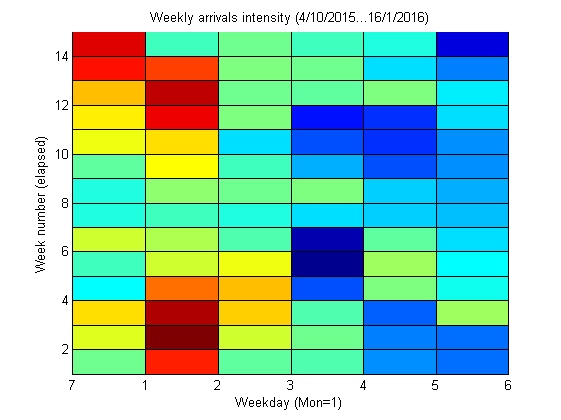
Figure 8: Daily arrivals grouped by week, illustrating days of various influx intensity, from low (blue) to high (red).

The plots in Figure 8 and Figure 9 demonstrate a clear difference in the influx intensity between various weeks and between various weekdays. Several external factors are associated to specific dates in this time frame, e.g. days of calm weather or political announcements related to the refugee crisis in Europe, which explain such differences at some level. In any case, it is clear that the first four weeks (early/mid-October 2015) and the last five weeks (mid-December 2015, early/mid January 2016) are characterized by the highest influx rates, with a relatively consistent preference in the Sunday/Monday 48-hour time frame.

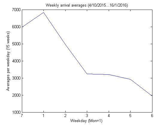
Figure 9: Weekday averages of daily arrivals.

IV Regression modeling

Two variants of the typical regression analysis are applied to the data series, in order to identify linear and periodic trends by predictive modeling.

IV-A Linear auto-regression

The linear regression approach [20, 22] is the most common and most basic model to formulate statistical dependencies between two series of data, usually an “input”, i.e., an external factor or control variable, and an “output”, i.e., an associated result. The most common formulation is:

$$\hat{y}\left(t\right)=\overrightarrow{b_{k}}\cdot\overrightarrow{u_{k}}\left(t\right)+e\left(t\right)$$ (1)

where $\overrightarrow{u_{k}}\left(t\right)$ is the input vector of size $k$ at time step $t$, $\overrightarrow{b_{k}}$ is the (static) vector of regression coefficients, $\hat{y}\left(t\right)$ is the estimated output and $e\left(t\right)$ is the model error at time step $t$, i.e., $e\left(t\right)=\left\|\hat{y}\left(t\right)-y\left(t\right)\right\|^{2}$. When there is no evident input and $y\left(t\right)$ is the data series of the output generated by an unknown process, then the input vector corresponds to some of the previous output values, typically a fixed-length window:

$$\overrightarrow{u_{k}}\left(t\right)\triangleq\overrightarrow{u_{n}}\left(t\right)=\left\langle y\left(t\right),y\left(t-1\right),\ldots,y\left(t-n+1\right)\right\rangle$$ (2)

where $\overrightarrow{u_{n}}\left(t\right)$ is the vector that consists of the current plus $n-1$ previous outputs.

In this study, a linear auto-regression model as in Eq.1 was introduced to approximate the daily arrivals, using an auto-regressive window as in Eq.2 with fixed length $n=13$ days as the input. The best-fit model was:

$$\begin{array}[]{cc}\hat{y}_{n}\backsimeq&1294.1+1.168\cdot y_{n-1}-0.458\cdot y_{n-2}\\ &+0.315\cdot y_{n-3}-0.287\cdot y_{n-4}\\ &+0.144\cdot y_{n-10}+0.155\cdot y_{n-11}+\ldots\end{array}$$ (3)

with Mean Absolute Prediction Error (MAPE): $err_{MAPE}=E\left[\left|e\left(t\right)\right|\right]=771.3$ and Root Mean Squared Error (RMSE): $err_{RMSE}=\sqrt{E\left[e\left(t\right)^{2}\right]}=1009.2$ [20], where the errors represent true output values (daily arrivals).

In this model, the most interesting factor is not the prediction accuracy per se, but the identification of the largest regression coefficients. Specifically, the result in Eq.3 shows that the spot value of the daily arrivals at any time step is associated primarily with the spot values of the four previous days and the values 10 and 11 days before, i.e., not so much by the values of the time frame 5-9 days before. This finding is a hint of a possible periodic behavior in the data series that needs further investigation with appropriate non-linear (periodic) components in the regression model. The following section enhances the model of Eq.1 with such factors and identifies the predominant periodic trends in the data.

IV-B Cosine-linear regression

In order to identify the periodicity of the data series of daily arrivals, a cosine term is introduced in the model of Eq.1, resulting in the new cosine-linear regression model:

$$\hat{y}\left(t\right)=\left(a\cdot\cos\left(b\cdot t+c\right)\right)+\left(d\cdot t+c_{0}\right)$$ (4)

where $d$ and $c_{0}$ define a standard linear component as in Eq.1, whereas $a$, $b$ and $c$ define the cosine component. In particular, $a$ is the scaling parameter, $b$ is the periodic parameter and $c$ is the corresponding phase. Here, the time sequencing parameter $t$ is the only input introduced in the model, in contrast to Eq.1 where previous values of the data series itself were used as input (hence the term auto-regression).

Using the cosine-linear regression model of Eq.10, the best-fit parameters where calculated as follows:

$$\hat{y}\left(t\right)=\left(875\cdot\cos\left(0.97\cdot t-2.85\right)\right)+\left(-47\cdot t+6669\right)$$ (5)

that is: $a\backsimeq 875.2$, $b\backsimeq 0.968$, $c\backsimeq-2.851$, $d\backsimeq-47.065$ and $c_{0}\backsimeq 6669.5$, optimal in the sense of Sum of Squared Errors (SSE) [20].

As with the simple linear auto-regression of Eq.3, the most interesting factor here is the values of the parameters, rather that the absolute prediction error. In particular, the predominant periodic trend, i.e., the major “period” of the daily arrivals, can be calculated from the periodic parameter $b$ as: $T_{C}=\nicefrac{{2\pi}}{{b}}\backsimeq 6.5$ (days). The linear trend or “slope” of the data series is the parameter $d=-47$, which is “downward”. This translates to 47 fewer arrivals each day, i.e., roughly equivalent to just one boat less. Figure 10 illustrates the true and the best-fit cosine-linear regression model as described in Eq.5.

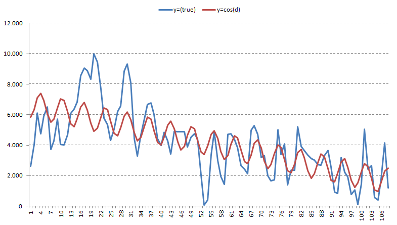
Figure 10: Comparison of true and predicted daily arrivals, using the best-fit (SSE) cosine-linear regression model of Eq.5.

V Spectral analysis

One of the most common approaches in analyzing the periodic properties of a signal is spectral decomposition via the Fourier transformation, specifically the Discrete Fourier Transform (DFT) or most commonly the Fast Fourier Transform (FFT) for discrete-valued signals [23, 24, 25, 26, 27, 28]. It is the most popular way of approximating a data sequence, structured in the time domain, by a series of sine and cosine components, structured in the frequency domain. In this way, the same signal remains the same but its representation is translated into frequency components, making its spectral properties clear and detailed.

The DFT is defined as:

$$Y_{k}\triangleq\sum_{n=0}^{N-1}y_{n}\cdot e^{-i2\pi k\frac{n}{N}}\;,\;k\epsilon\mathbf{Z}$$ (6)

or, in analytical form:

$$Y_{k}\triangleq\sum_{n=0}^{N-1}y_{n}\cdot\left(\cos\left(-2\pi k\frac{n}{N}\right)+i\cdot\sin\left(-2\pi k\frac{n}{N}\right)\right)\;,\;k\epsilon\mathbf{Z}$$ (7)

where $y_{n}$ are the signal samples, $N$ is the size of the data series, $k$ is each frequency under consideration and $Y_{k}$ is the corresponding (complex) frequency component. Under DFT, the signal is considered periodic ($T=N$) and, due to the Nyquist-Shannon sampling theorem [23, 24], the (discrete) spectrum is “mirrored” around $\pi,$ hence the maximum identifiable frequency here is $\nicefrac{{N}}{{2}}$, which correspond to “changes per period”.

Figure 11 illustrates the spectral representation (FFT) of the complete data series of daily arrivals, using full resolution $\left(N=108\right)$. The blue line is the half-spectrum log-plot, i.e., the rightmost point (max) on the horizontal axis corresponds to $\omega=\pi$, while the red line is the corresponding moving average with window size 20.

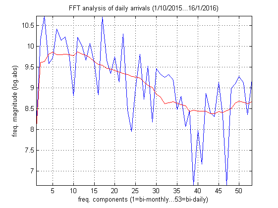
Figure 11: Spectral representation (FFT log-plot) of the complete data series of daily arrivals.

The spectral components in Figure 11, represented by each point on the horizontal axis, correspond to the full range of frequencies analyzed, from $f_{min}=\frac{1}{N}=\frac{1}{108}$ to $f_{max}=\frac{N/2}{N}=\frac{1}{2}$. This frequency range represents “changes” and it runs from one such “change” for the entire data series available ($T_{max}=N=108$ days) to the maximum resolution, which is half the entire size ($T_{min}=2$ days), according to Nyquist theorem [23, 24, 26]. Since the vertical axis is log-scaled, every +1 in value corresponds to 10 times larger energy in the specific component.

The size of the data series is relatively small, hence the spectral analysis in Figure 11 is useful for a qualitative, rather than quantitative assessment of the signal. However, the moving average highlights some important aspects, already identified by the preliminary analysis via linear and cosine-linear regression. Specifically, the power density profile illustrates a typical low-frequency signal, with most of its energy packed in the lower 1/3 of the FFT spectrum. The point where the moving average (red line) crosses downwards to energy magnitudes lower than 9.5 is roughly at $x_{L}=17.5$ on the horizontal axis; since it is scaled from $\left\{f_{min}:\>x_{min}=1\right\}$ to $\left\{f_{max}:\>x_{max}=\left\lceil\frac{108}{2}\right\rceil=54\right\}$ as described earlier, this point corresponds roughly to the rescaled point $f_{L}$ according to:

$$\begin{array}[]{cc}f_{L}&=\left(\frac{x_{L}-x_{min}}{x_{max}-x_{min}}\right)\cdot\left(f_{max}-f_{min}\right)+f_{min}\\ &=\left(\frac{17.5-1}{54-1}\right)\cdot\left(\frac{1}{2}-\frac{1}{108}\right)+\frac{1}{108}\\ &\simeq 0.162\end{array}$$ (8)

In other words, the daily arrivals signal is (for the most part) bounded by the upper frequency $f_{L}=0.162$ or, in terms of period, $T_{L}=\frac{1}{f_{L}}\simeq 6.1714$ (days). This limit is very close to the period $T_{C}=6.5$ identified by the cosine-linear regression model earlier, which strongly suggests that the data series is indeed periodic with a major period of almost (less than) a full week.

VI Auto-Regressive Moving-Average

The statistical and frequency properties of the daily arrivals data series was analyzed via pairwise correlation, phase diagrams and full system identification, specifically by Auto-Regressive Moving Average (ARMA) approximations, as described below.

VI-A Auto-correlation & phase

Pairwise correlation produces a quantitative metric for the statistical dependencies between values of two data series at different lags. In the case when a single data series is compared to itself, the auto-correlation corresponds to the statistical dependencies between subsequent values of the same series [27, 29]. Hence, value pairs with high correlation correspond to regular patterns in the series, i.e., encode periodicity at smaller or larger scales, according to the selected lag.

In this study, the daily arrivals were analyzed via auto-correlation with a lag limit of $k\pm 10$ against the current day. This limit was selected as appropriate after the preliminary analysis via regression modeling that confirmed strong periodicity and frequency components below the 7 days boundary (see above). Figure 12 presents the plot of the auto-correlation vector of the entire daily arrivals data series; the auto-correlation vector is symmetric around the central point ($k=0$), hence only the positive half-width plot ($1\leq k\leq 10$) is included here.

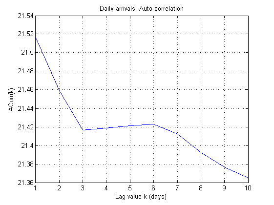
Figure 12: Auto-correlation plot of the daily arrivals for lag limit $k=\pm 10$.

A typical chaotic or semi-stochastic signal is expected to exhibit an exponentially decreasing profile in its auto-correlation plot: sharper “drop” of the profile as the lag value $k$ increases means smaller window of dependency between subsequent values, i.e., a higher-frequency signal. In contrast, lag values that present a curve higher than the expected asymptotically vanishing profile correspond to significant statistical dependencies at this scale, i.e., strong periodic trends.

As in the case of regression modeling, the auto-correlation plot in Figure 12 reveals strong periodic trends around the 6-days threshold. It also reveals strong low-frequency energy profile, since it exhibits a distinct high peak at $k=1$ and exponentially decreasing gradually to $k=3$; this means that daily arrivals are strongly related to previous values of up to three days. The plot also shows that this strong dependencies remain valid for at least six days in total.

Figure 13 presents the phase diagrams of the entire daily arrivals data series, i.e., the 2-D plot of subsequent values $y\left(t\right)$ against $y\left(t+k\right)$, scaled down by 100 and separated by different lag values of up to nine days ($1\leq k\leq 9$). Each pair is presented by a dot (blue), while the diagonal line (red) corresponds to the symmetric boundary of $k=0$.

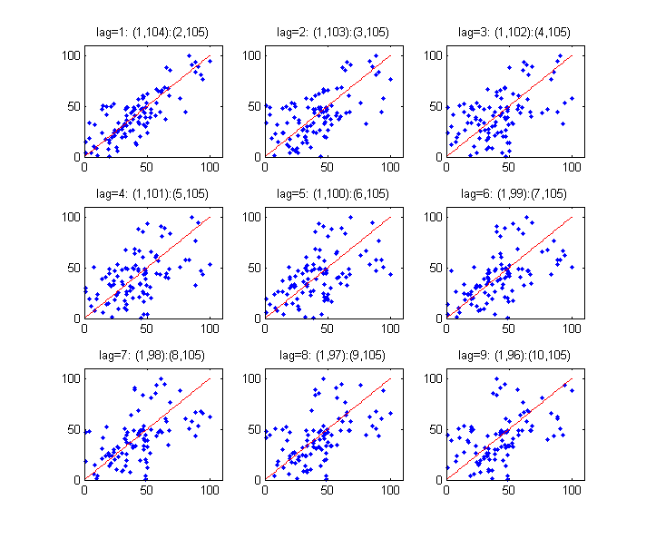
Figure 13: Phase diagrams of the daily arrivals for lag limit $k=\pm 9$.

In accordance to the auto-correlation plots, strong statistical dependencies between value pairs in the signal appear as clusters; the closer they are to the symmetric boundary, the smaller is the lag separation between similar values. In other words, a low-frequency signal appears with most value pairs “packed” around the symmetric boundary. The exact frequency components of the signal (spectral profile) affect how this distribution “spreads” wider around the symmetric boundary as the lag value increases, i.e., the separation between the values of each pair.

Although the phase plots in Figure 13 are not conclusive in a similar way as with the auto-correlation plot in Figure 12, it is evident that the plot for a one-day lag ($k=1$) is clearly more “packed” around the symmetric boundary than in any other lag value. In accordance to the basic statistics presented earlier in Figure 7 and Table I, the clusters in all plots appear more dense below the value 60 (i.e., less than 6,000 arrivals a day). Furthermore, within that range, a somewhat tighter “packing”, similar to the one for $k=1$, reappears when $5<k<8$; again, evidence that there is some periodic trend within that range (lag in days).

VI-B ARMA system identification

More generic and powerful than auto-correlation or linear regression alone, the Auto-Regressive Moving Average (ARMA) model is the standard approach for describing any linear digital filter or signal generator in the time domain. It is essentially a combination of an auto-correlation component that relates the current outputs to previous ones and a smoothing component than averages the inputs over a fixed-size window.

The typical linear ARMA model is described as [29, 30, 25, 22]:

$$A_{m}\left(z\right)\ast\overrightarrow{y}\left(t\right)=B_{k}\left(z\right)\ast\overrightarrow{u}\left(t\right)+e\left(t\right)$$ (9)

where $\overrightarrow{u_{k}}\left(t\right)$ is the input vector of size $k$ at time step $t$, $\overrightarrow{y}\left(t\right)$ is the output vector of size $m$ (i.e., the current plus the $m-1$ previous ones), $B_{k}\left(z\right)$ is the convolution kernel for the inputs, $A_{m}\left(z\right)$ is the convolution kernel for the outputs and $e\left(t\right)$ is the residual model error. Normally, $A_{m}\left(z\right)$ and $B_{k}\left(z\right)$ are vectors of scalar coefficients that can be fixed, if the model is static, or variable, if the model is adaptive (constantly “retrained”).

Both coefficient vectors, as well as their sizes, are subject to optimization of the model design according to some criterion, which typically is the minimization of the residual error $e\left(t\right)$. In practice, this is defined as $e\left(t\right)=\left\|\hat{y}\left(t\right)-y\left(t\right)\right\|^{2}$, where $\hat{y}\left(t\right)$ is the ARMA-approximated output and $y\left(t\right)$ is the true (measured) process output. The sizes $m$ and $k$ are the orders of the model and they are usually estimated either by information-theoretic algorithms [29, 30, 22] or by exploiting known properties (if any) of the generating process, e.g. with regard to its periodicity. Such a model is described as ARMA($m$,$k$), where AR($m$) is the auto-regressive component and MA($k$) is the moving-average component.

In approximation form, expanding the convolutions and estimating the current output $\hat{y}\left(t\right)$, the analytical form of Eq.9 is:

$$\hat{y}\left(t\right)=\sum_{i=1}^{m}\left(a_{i}\cdot y\left(t-i\right)\right)+\sum_{j=0}^{k}\left(b_{j}\cdot x\left(t-j\right)\right)+e\left(t\right)$$ (10)

The error term $e\left(t\right)$ in Eq.10 can also be expanded to multiple terms of a separate convolution kernel, similarly to $A_{m}\left(z\right)$ and $B_{k}\left(z\right)$, but it is most commonly grouped into one scalar factor, i.e., with an order of one. In such cases, the model and be described as ARMA($m$,$k$,$q$) where $q>1$ is the order of the convolution kernel for the error term.

When applied to a signal generated by a process of unknown statistical properties, an ARMA approximation of it reveals a variety of important properties regarding this process. In practice, the (estimated) order $m$ of the AR component shows how strong the statistical coupling is between subsequent outputs, while the order $k$ of the MA component shows the “memory” of the process, i.e., how far in the past inputs the process “sees” in order to produce the current output.

In the current study, preliminary analysis via auto-correlation, linear regression and cosine-linear regression (see previous sections) has revealed strong periodic components that can be exploited here. Additionally, the ARMA models were designed and trained using arbitrary ranges for their orders to verify and optimize the initial choices.

Several ARMA models where designed and optimized for approximating the daily arrivals data series for exploring the necessary orders and the distribution of magnitude in the corresponding coefficient vectors. Since the daily arrivals is inherently an auto-regressive process, with each spot value depending heavily on the values of the previous days, the tested orders for the AR where bounded between 1 (just the previous day) and 21 (three full weeks back); the weekday was used as the input with MA order of 1 (no averaging over repeating weekday cycles); and the error term was modeled with convolution kernels of orders up to 3.

Using an ARMA(9,1,3) model, the optimal approximation of the daily arrivals yields:

$$\begin{array}[]{cc}A_{9}\left(z\right)&=1-0.8887\cdot z^{-1}+0.1247\cdot z^{-2}+0.2971\cdot z^{-3}\\ &-0.3747\cdot z^{-4}+0.1526\cdot z^{-5}-0.1265\cdot z^{-6}\\ &-0.1357\cdot z^{-7}+0.164\cdot z^{-8}-0.144\cdot z^{-9}\end{array}$$ (11)

and:

$$B_{9}\left(z\right)=48.94\cdot z^{-3}$$ (12)

The $A_{9}\left(z\right)$ and $B_{9}\left(z\right)$ polynomials are the (optimal) convolution kernels for the AR(9) and MA(1) components, respectively. In both polynomials, $z^{-n}$ is the delay factor of the kernel, as described by the analytical form of Eq.10. Hence, the coefficient of $z^{-n}$ in $A_{9}\left(z\right)$ is essentially $a_{n}$, i.e., the magnitude for the auto-regressive factor (output) $n$ days back.

The most important results from Eq.11 are: (a) the $z^{-1}$ coefficient is the largest and very close to 1, signifying strong low-frequency spectral components, and (b) the $z^{-3}$ and $z^{-4}$ coefficients are at least twice as large as any other coefficient in this AR(9) convolution kernel, signifying strong within-week periodic trends in the daily arrivals. Figure 14 presents the AR(9) coefficients and illustrates the clear increase in magnitude of these two coefficients at lags 4 and 5.

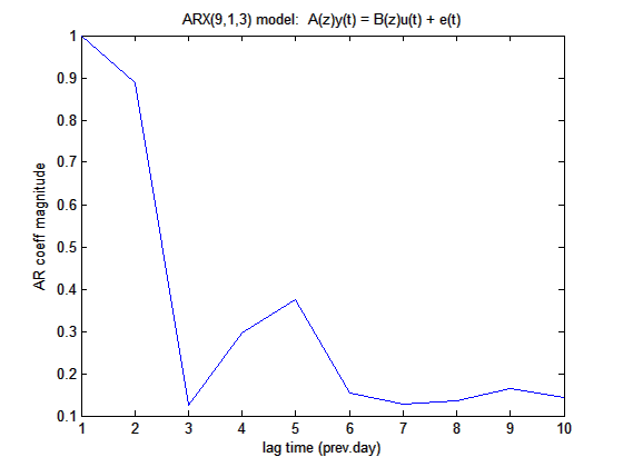
Figure 14: Magnitude (abs) plot of the convolution kernel of Eq.11; horizontal axis is: $\left[1,A_{9}+1\right]$.

While the ARMA(9,1,3) approximation is useful for evaluating the weekly time frames, a more complex model was also applied for a better minimal-error approximation of the daily arrivals. Specifically, an ARMA(21,1,1) was estimated for a full three-week time frame for AR with singular MA and error convolution kernels. In this case, the optimal model design yields:

$$\begin{array}[]{cc}A_{21}\left(z\right)&=1-1.608\cdot z^{-1}+0.9277\cdot z^{-2}+0.3233\cdot z^{-3}\\ &-1.142\cdot z^{-4}+0.9955\cdot z^{-5}-0.4887\cdot z^{-6}\\ &-0.1842\cdot z^{-7}+0.4908\cdot z^{-8}-0.4291\cdot z^{-9}\\ &-0.02225\cdot z^{-10}+0.235\cdot z^{-11}-0.1331\cdot z^{-12}\\ &-0.1298\cdot z^{-13}+0.1242\cdot z^{-14}-0.0892\cdot z^{-15}\\ &+0.2391\cdot z^{-16}-0.3209\cdot z^{-17}+0.4167\cdot z^{-18}\\ &-0.4449\cdot z^{-19}+0.1795\cdot z^{-20}+0.1159\cdot z^{-21}\end{array}$$ (13)

and:

$$B_{21}\left(z\right)=57.98\cdot z^{-1}$$ (14)

As in the case of the AR(9) component in Eq.11, this AR(21) component in Eq.13 reveals very useful information about the generating process. More specifically, it is clear that: (a) the magnitude of all coefficients fade asymptotically as the lag increases, signifying a signal with strong low-frequency spectral components, and (b) there is a clear pattern of alternating larger and smaller magnitudes in the components, signifying periodic trends within a window smaller than the order of AR(21).

Figure 15 presents the AR(21) coefficients and verifies these observations regarding the distribution of magnitudes. In this case, the peaks are at lags 2, {5,6}, {9,10}, etc. There is also evidence of longer-term dependencies beyond lag 18 (end of 3rd week in the time frame), although in many cases such patterns may be related to noise or other approximation artifacts rather than the generating process itself.

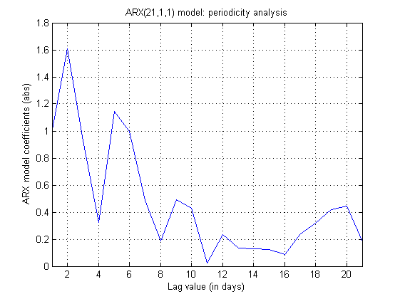
Figure 15: Magnitude (abs) plot of the convolution kernel of Eq.13; horizontal axis is: $\left[1,A_{21}+1\right]$.

Figure 16 presents three ARMA model approximations of the daily arrivals with different AR orders. Specifically, a one-week ARMA(7,1,3) (gray), a two-week ARMA(14,1,1) (olive) and a three-week ARMA(21,1,1) (red) is presented against the true data series of the daily arrivals (black). It is clear that, as the AR order increases, the approximation becomes better and more detailed than the general trend. These results show that an AR(21), i.e., a three-week auto-regressive model, can produce a practically usable formulation for the short-term forecasting of daily arrivals.

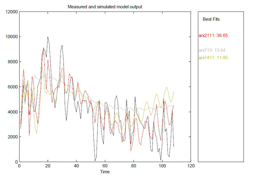
Figure 16: Comparative plot of one-week ARMA(7,1,3) (gray), two-week ARMA(14,1,1) (olive) and three-week ARMA(21,1,1) (red) approximation models for the daily arrivals data series (black).

VII Matrix factorization - Component analysis

Spectral decomposition and frequency analysis of a signal often involves some transformation to the spectral domain, as it was described earlier for FFT with Eq.6 and Eq.7. An alternative approach is to reformulate the original signal into a matrix form and assume multiple signals of shorter size, in order to analyze their similarities in the spectral domain. This is typically conducted by some form of Matrix Factorization (MF) that expresses the original matrix as a product of two other matrices, the “spectral components” and the corresponding coefficients. In the context of system identification, MF can be used as a very powerful tool for discovering the periodic trends and the spectral properties of the original signal and, hence, the generating process in question.

In this study, MF was employed for spectral decomposition of the daily arrivals in various forms, including SVD, PPCA, ICA and K-SVD, as described below.

VII-A SVD

The Singular Value Decomposition (SVD) [20] of a matrix is one of the most widely used algorithms in Linear Algebra with regard to rank and dimensionality reduction. Given a $l\times n$ matrix $Y$ of rank $r\leq\min\left\{l,n\right\}$, SVD transforms it to a product as:

$$Y=U\cdot\left[\begin{array}[]{cc}A^{\frac{1}{2}}&O\\ O&0\end{array}\right]\cdot V^{H}$$ (15)

where $A^{\frac{1}{2}}$ is the $r\times r$ diagonal matrix with elements $\sqrt{\lambda_{k}}$, and $\lambda_{k}$ are the $r$ non-zero eigenvalues of the associated matrix $Y^{H}\cdot Y$. In other words, SVD transforms the original matrix $Y$ into a special diagonal form that includes the eigenvalues, which provide a very useful description of its “spectral” components included in the eigenvector matrices $U$ and $V$. This approach is being widely used for decades in Pattern Recognition for a variety of applications, from signal compression and dimensionality reduction to feature generation and image coding [20, 31, 32].

In this study, the daily arrivals data series was restructured into a weekly-grouped version of a slightly truncated version (15x7 = 105 days), as it is illustrated in Figure 8. The purpose here is to decompose the data series into “weekly trends” via SVD, according to Eq.15, and investigate the significance of each individual component. Instead of examining the eigenvalues in the corresponding matrix $A^{\frac{1}{2}}$, the original data series is approximated by using 1 to 7 (all) SVD components, in order to estimate their relative “coding” efficiency. Figure 17 illustrates this approach, with the top-level sub-plot referring to reconstruction by only the first (rank-1) SVD component and subsequent sub-plots referring to reconstructions by increasing number of components up to 7 (full-rank). The bottom-right histogram illustrates the corresponding SVD components ranked according to their spectral energy.

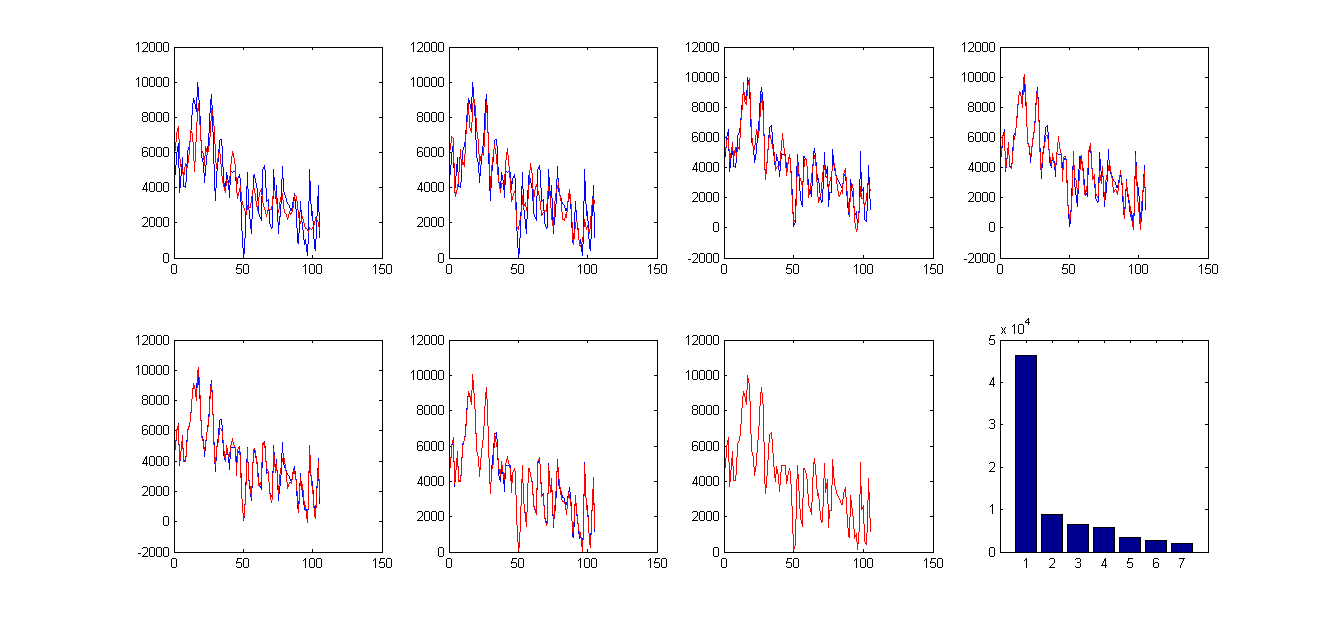
Figure 17: SVD spectral approximation (red) of the weekly-grouped arrivals, plotted against the true data series (blue); the horizontal axis is the time (days); the histogram at the bottom-right corner is the same components ranked according to their spectral energy.

It is clear from the results in Figure 17 that the daily arrivals is a signal with strong low-frequency signature. The histogram, as well as the first row of sub-plots, illustrate that the data series can be approximated effectively by the three or four major spectral components. This means that if a predictive model is required, the corresponding eigenvectors and eigenvalues calculated by SVD can be used for rank-3 or rank-4 approximations, respectively, for robust and noise-resilient forecasting.

VII-B PPCA

In Linear Algebra, Principal Component Analysis (PCA) is a MF algorithm for expressing a matrix as a result of orthogonal projections. In practice, it is a statistical procedure that uses an orthogonal linear transformation of a set of observations into a set of values of linearly uncorrelated variables, called principal components. The PCA algorithm is formally known as Karhunen-Loeve Transform (KLT) [20] and, like SVD, it is being used for many years in Pattern Recognition for signal coding, dimensionality reduction, feature generation, etc.

Formally, the KLT is defined as:

$$P=Y\cdot W\>\Leftrightarrow\>Y=P\cdot W^{H}$$ (16)

where $P$ is the “loading vectors” matrix, $Y$ is the original data matrix and $W$ is the matrix whose columns are the eigenvectors of $Y^{H}\cdot Y$. It is clear from Eq.15 and Eq.16 that KLT is closely related to SVD, as both of them involve the corresponding eigenvectors, i.e., they employ orthogonal projections that are error-optimal in the mean-square-error (MSE) sense. This means that, as with SVD (which is more general), if only some of the “spectral” components are to be used for MSE-optimal approximation of the original data, Eq.16 can be used with the matrix $W$ truncated as to include only the first $k$ eigenvectors (“basis” columns).

The Probabilistic Principal Component Analysis (PPCA) [33] is an extension to PCA in the sense that it includes a parametric probabilistic model for the signal (typically Gaussian, estimated via Maximum Likelihood). This provides an efficient way to deal with missing data, outliers and increased noise resiliency. The KLT formulation is extended to include non-zero mean $\mu$ and residual error $\varepsilon$:

$$Y=P\cdot W^{H}+\mu+\varepsilon$$ (17)

In this study, PPCA was used in a similar way as with SVD described earlier, i.e, the daily arrivals data series was restructured into a weekly-grouped version of a slightly truncated version (15x7 = 105 days), as it is illustrated in Figure 8. This means that the data matrix $Y$ was analyzed for “weekly trends”, employing a full-rank MF according to Eq.17. Figure 18 illustrates these components, which essentially are the contents of the resulting matrix $W^{H}$.

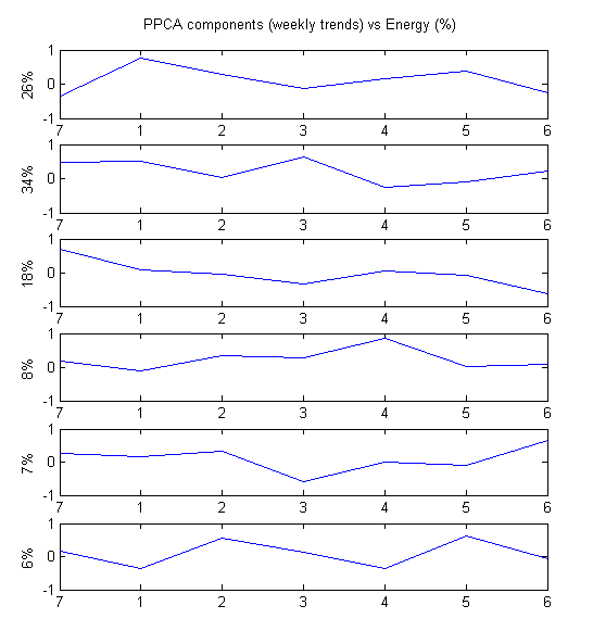
Figure 18: PPCA components of the weekly-grouped daily arrivals; horizontal axis is the weekdays; % labels in the left show the relative variance (energy) described by each component.

The percentage labels on the left of each sub-plot in Figure 18 represent the relative variance described by each component; in other words, how much of the total energy of the signal is included when it is reconstructed by each single component. Hence, each of these “weekly trends” constitutes a compact set of spectral descriptors of the original signal. As in the case of SVD, using only three of these components is enough to describe almost $\nicefrac{{3}}{{4}}$ (78%) of the energy content of the data series.

VII-C ICA

The PCA and Probabilistic PCA methods that were presented earlier are based on orthogonal linear transformations that are error-optimal in the MSE sense [33]. However, there are cases were making the transformed data statistically uncorrelated, as the KLT does, is not adequate to create an effective mapping to a new, more efficient space. Instead, alternative methods have to be employed in order to make the data statistically independent - a much stronger requirement.

The Independent Component Analysis (ICA) is a family of algorithms and statistical methods for transforming a set of data into a mixture of statistically independent components, usually in the context of blind source separation (BSS) tasks [34, 35, 36, 37]. More specifically, ICA can be viewed under the scope of MF as [38, 39, 20]:

$$Y=A\cdot S$$ (18)

where $Y$ is a $l\times n$ matrix of observations, i.e., $l$ measurements for each of $n$ variables, $A$ is a $l\times k$ “mixture” matrix and $S$ is a $k\times n$ matrix of $k$ statistically independent “sources”.

ICA has been used successfully in a wide range of data-intensive processing tasks, from big data and data mining to fMRI unmixing [40, 41, 42, 43]. It is based on identifying non-Gaussian properties between the sources and separating them from the mixture, essentially reconstructing the original signal as a linear combination of identified components. Naturally, the number of independent sources is bounded by the maximum column-rank of matrix $Y$, i.e., $k\leq n$. In other words, the original data are assumed to be generated by $k$ independent processes from which only one may be Gaussian. The constraint of statistical independency is defined via a non-linearity metric, usually kurtosis or hyperbolic tangent functions.

In this study, ICA was used in a similar way as with SVD and PPCA described earlier, i.e, the daily arrivals data series was restructured into a weekly-grouped version of a slightly truncated version (15x7 = 105 days), as it is illustrated in Figure 8. The data matrix $Y$ was analyzed via ICA for “weekly trends”, here in the context of generating “sources”, i.e., weekly patterns or “templates” that are statistically independent.

The ICA processing was conducted with the fastICA toolbox 2.5 for Matlab [44], implementing the Hyvarinen’s fixed-point algorithm [45, 46]. The fastICA has been used in various studies [47] as a benchmark for the ICA family of algorithms for BSS, with different choices regarding the exact non-linearity and decorrelation approach. In this study, all four non-linearity choices were considered, namely pow3, Gaussian, skewness and hyperbolic tangent, since previous studies have used different choices as optimal. Additionally, both decorrelation approaches were used, namely symmetric (estimate all the independent components simultaneously) and iterative (estimate independent components one-by-one like in projection pursuit). In all cases, a standard PCA pre-processing stage was included.

Similarly to the SVD and PPCA analysis for MF, here the daily arrivals data series was restructured into a weekly-grouped version of a slightly truncated version (15x7 = 105 days), as it is illustrated in Figure 8. The purpose here is to decompose the data series into “weekly trends” via ICA, i.e., as mixtures of statistically independent (not just uncorrelated) components, according to Eq.18. The significance of each individual ICA component was investigated by means of reconstruction error, as well as the signal energy captured by the variance in each case.

Since the structure of the data matrix the $Y$ in Eq.18 hints a maximum column-rank of seven, Figure 19 illustrates the first six ICA components as weekly trends, while the seventh component is simply the residual reconstruction error. From this plot, it is evident that there are indeed several distinct “templates” of weekly trends for the daily arrivals. The relevance of each one of these patterns are quantified by the individual rank-1 reconstruction and comparison of the resulting signal to the original data series of daily arrivals in terms of energy.

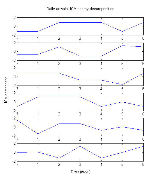
Figure 19: fastICA components (tanh non-linearity, symmetric decorrelation) of the weekly-grouped daily arrivals; horizontal axis is the weekdays.

Figure 20 illustrates the distribution of the ICA components (see: Figure 19) of the weekly-grouped daily arrivals, plotted against their relative (%) spectral energy. It is evident that the third component (from top) dominates the energy distribution histogram and along with the fourth component correspond almost to $\nicefrac{{2}}{{3}}$ of the signal energy of the original data series. Although in general the ICA components are not directly interpretable with regard to the original domain of the signal, these findings explain and further support the statement that there are clear periodic trends in the daily arrivals that correspond to short “bursts” and somewhat longer “pauses”, as previous spectral and MF methods also suggest.

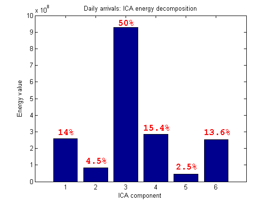
Figure 20: Distribution of the fastICA components (see: Figure 19) of the weekly-grouped daily arrivals, plotted against their relative (%) spectral energy.

Figure 21 illustrates the true and the rank-6 (incomplete) ICA reconstruction of the weekly-grouped daily arrivals (red), plotted against the true data series (blue); the horizontal axis is the time (days).

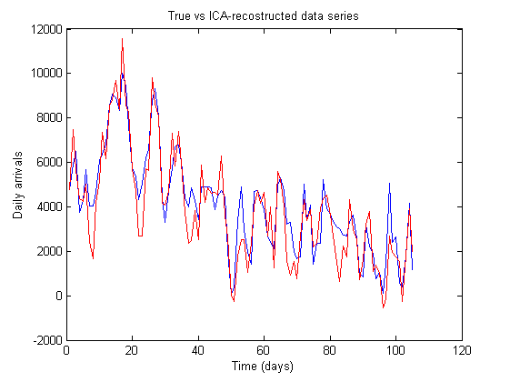
Figure 21: Plot of the fastICA reconstruction of the weekly-grouped daily arrivals (red) against the true data series (blue); the horizontal axis is the time (days).

VII-D K-SVD

The SVD, PPCA and ICA methods for MF that were presented earlier can all be referred to as full-rank algorithms: unless the original matrix $Y$ is inherently rank-deficient by structure, these methods produce a MF formulation that exploits this full-rank property, i.e., utilizes the maximum number of components for the mixture. Hence, in the case of the daily arrivals data series restructured here into a weekly-grouped matrix version as in Figure 8, any similar full-rank MF will produce a maximum of seven components.

A recent and very different approach to the MF problem is the introduction of additional constraints to the task, specifically in the structure of the components matrix. Instead of putting statistical decorrelation or independency, the original data are formulated as a sparse mixture of dictionary elements, in a similar way:

$$Y^{T}=D\cdot C$$ (19)

where $Y$ is a $l\times n$ matrix of observations, i.e., $l$ measurements for each of $n$ variables, $D$ is a $l\times k$ “dictionary” of $k$ elements (columns) and $C$ is the corresponding $k\times n$ matrix coefficients that define the mixture [48, 49].

Although the MF formulation here looks the same as in the previous methods, Eq.19 defines the mixture for $Y$ as a product of a dictionary $D$ of components and a coefficient matrix $C$. The idea is to use as little components from $D$ as possible to reconstruct the original data. In practice this means that the additional constraint is to have as many zeros as possible in every column of matrix $C$, as this is equivalent to canceling out the corresponding dictionary elements. For example, if $C_{*,j}=\left[0,1,0,0,-2,4,0\right]^{T}$ then only the three non-zero coefficients will be used in the mixture (product) with the dictionary $D$ to produce the current element (of column/variable $j$) of the data matrix $Y$.

The dictionary $D$ may be over-complete, which means that at most $m\leq k$ elements may be used in the mixture but there is no strict rank-related limit to the actual number of elements (columns) in the dictionary, other than being able to produce a more “packed” representation of the original signal. This is established in practice by combing sparsity in the coefficients and incoherency (e.g. decorrelation) in the dictionary elements. Although this seems equivalent to what SVD or (P)PCA does in practice, here the incoherency metric can be any function than compares the “similarity” between the elements (columns) in dictionary $D$. Both sparsity and incoherency constraints define the exact size $k$ in Eq.19 and they are a key property that has been studied extensively over the last few years.

In Eq.19, the dictionary $D$ can be pre-defined as a set of general-purpose functions that can produce an effective spectral decomposition of the original signal - usually an over-complete set of trigonometric of wavelet functions. This is not much different than the standard Discrete Wavelet Transformation (DWT), only now there is no inherent multi-scale property and the dictionary elements do not have to be rescaled variants of the same detail or approximation wavelet. If properly configured, DWT may also produce a sparse or compressed spectral representation of a signal, however here the sparsity constraint is explicitly defined in the decomposition algorithm, normally via the $l_{0}$ norm or (in practice) via the $l_{1}$ norm and variants (e.g. see: LASSO [50]). For proper sparse decomposition, the dictionary $D$ must also be defined in a data-driven way, i.e, learned by the data, instead of being pre-defined a priori. Hence, these approaches are referred to as Dictionary Learning (DL) algorithms and they are currently in the state-of-the-art in the context of the general BSS task, as well as in Coding Theory, with a wide range of applications including Compressed Sensing (CS), wireless sensor networks, fMRI & EEG analysis, etc [36, 51, 52, 53, 54].

The K-SVD algorithm is one of the most popular approaches in the standard DL task. In practice, it implements the formulation of Eq.19 by alternating training steps of the dictionary $D$ and the coefficients $C$. More specifically, it produces a rank-1 approximation of the residual reconstruction error, uses it to update the matrix $D$, then uses this new updated dictionary to produce a new mixture $C$, repeating this cycle iteratively until a specific average sparsity constraint is satisfied and/or the total reconstruction error becomes smaller than a specific threshold. Due to its flexibility in terms of defining sparsity and incoherency, K-SVD has been widely adapted to various problem-specific tasks, e.g. allowing some limited number of non-sparse elements in $D$ to be used in order to capture noise/artifacts, background elements, etc [52, 55, 56, 57, 58]. Other sparsity-promoting approaches include Non-Negative Least Squares (NNLS) approximations, without the $l_{1}$ norm [59, 60, 61], as well as special versions of ICA or DL with additional “structural” constraints on the produced MF approximation [51, 62, 40].

In this study, K-SVD was used to produce a MF formulation in the context of DL, similarly to the ones produced by the other MF methods presented earlier. Again, the daily arrivals data series was restructured into a weekly-grouped version of a slightly truncated version (15x7 = 105 days), as it is illustrated in Figure 8. The DL approach was employed to analyze the data matrix $Y$ for “weekly trends”, which are encoded as the elements of the dictionary $D$. For practical reasons, Eq.19 shows that the data matrix $Y$ was used transposed, in order for dictionary $D$ to produce weekly-based components. Figure 22 shows the K-SVD components (columns of $D$) of the weekly-grouped daily arrivals; horizontal axis is the weekdays; the histogram at the bottom-right corner is the same components ranked according to their relative spectral energy.

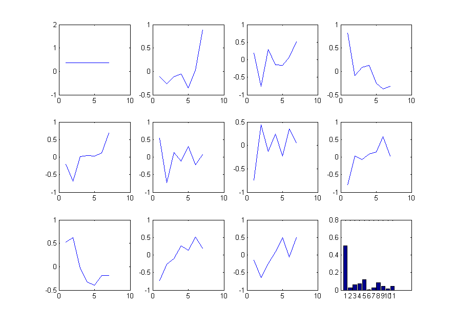
Figure 22: K-SVD components (dictionary) of the weekly-grouped daily arrivals; horizontal axis is the weekdays; the histogram at the bottom-right corner is the same components ranked according to their relative spectral energy (dictionary size = 11, sparsity constraint = 7, reconstruction error = 2.e-12).

Figure 23 illustrates the K-SVD spectral approximation (red) of the weekly-grouped arrivals, plotted against the true data series (blue); the horizontal axis is the time (days). Each individual plot corresponds to data series reconstruction that uses one additional mixture element, i.e., from $k=1$ to $k=11$. In each case, $m\leq\max\left\{k,7\right\}$ corresponds to the number of elements used from the dictionary $D$ of size $k$, which are sorted against their overall contribution (energy) in the reconstructed signal; in other words, each reconstruction uses a larger set of energy-sorted elements from $D$ and, hence, produces a smaller reconstruction error. For the maximum sparsity constraint of $m=7$ and the full dictionary size $k=11$, perfect reconstruction is achieved.

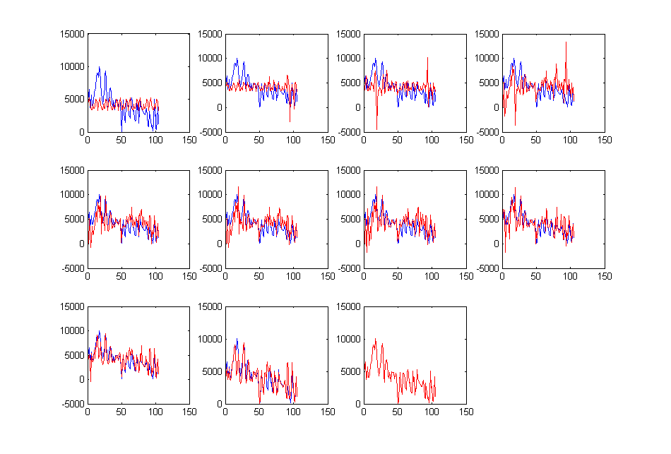
Figure 23: K-SVD spectral approximation (red) of the weekly-grouped arrivals, plotted against the true data series (blue); the horizontal axis is the time (days) (dictionary size = 11, sparsity constraint = 7, reconstruction error = 2.e-12).

It is clear from Figure 23 that K-SVD can produce a very accurate representation of the daily arrivals data series by using a rank-7 mixture and at least 11 dictionary elements. Although this seems a more complex model compared to the previous MF approaches, these plots show that even from a dictionary of five the reconstruction quality is already comparable to the other methods. The reason that the reconstruction becomes perfect only when the size becomes maximum $\left(k=11\right)$ is that the mixture is based on a sparse representation and not all dictionary elements are used equally. This is more evident, in a quantitative way, in the right-bottom histogram subplot in Figure 22, where the first or “background” component contributes roughly 50% of the energy of the original signal - exactly as it was described earlier for ICA in Figure 20 (third component). However, the top-left subplot in Figure 22 reveals that in this case the corresponding component is “flat” (constant). The remaining energy is spread in the rest of the components, but in this case their total number is 10 instead of six and, hence, the maximum relative contribution is roughly 10% instead of 13-15% as in ICA.

VIII Fractal dimension analysis

In recent years, dimensionality analysis in signal processing has been extensively linked to fractal analysis and fractal dimension, as a non-parametric method for the quantitative characterization of the complexity or “randomness” of a signal [63, 64]. When applied to 1-D signals, metrics like the Hurst exponent and the Lyapunov exponent have been used as statistical features to describe various types of data series, from biomedical signals (e.g. EEG, ECG, etc) to financial and climate time series. In 2-D signals, these methods provide additional features for characterizing the texture of images, e.g. when analyzing biomedical modalities (radiology, ultrasound, MRI, etc) [65]. Fractal dimension is closely linked to these fractal parameters and it provides a clear distinction between the embedding space, i.e., the full-rank space in the algebraic sense, from the actual space spanned by the registered sensory data. In the general case when fractal analysis is applied to some multi-dimensional signal, the estimation of the fractal dimension can be used as a realistic evaluation of the “complexity” of the space spanned by the actual data points available and, hence, a very useful hint regarding the inherent redundancy in a given data set.

In order to establish a preliminary estimation of the complexity and intrinsic dimensionality of data sets, fractal analysis provides a data-centric approach for this task. Data set fractal analysis, specifically the calculation of intrinsic fractal dimension (FD) of a data set, provides the quantitative means of investigating the non-linearity and the correlation between the available features (i.e., dimensions) in terms of dimensionality of the embedding space [65, 66].

In the case of data series, as the daily arrivals in this study, there are algorithms designed specifically for fast approximation of the FD in terms of the Hurst or Lyapunov exponents. However, the most generic approach is to treat the measurements of the data series as an arbitrary data set with dimension of two or one, if represented as $\left(x,y\right)$ pairs or single-valued, respectively, and process it via dataset-oriented algorithms for estimating the FD. The two most commonly used methods of calculating the FD in such cases are the pair-count ($PC$) and the box-counting ($BC$) algorithms [64, 66, 67, 63]. In the PC algorithm, all Euclidean distances between the samples of the data set are calculated and a closure measure is then used to cluster the resulting distances space into groups, according to various ranges $r$, i.e., the maximum allowable distance within samples of the same group. The $PC$ value is calculated for various sizes of $r$ and it has been proved that $PC\left(r\right)$ can be approximated by:

$$PC\left(r\right)=K\cdot r^{D}$$ (20)

where $K$ is a constant and $D$ is called PC exponent. The $PC\left(r\right)$ plot is then a plot of $log\left(PC\left(r\right)\right)$ versus $log\left(\nicefrac{{1}}{{r}}\right)$, i.e., $D$ is the slope of the linear part of the $PC\left(r\right)$ plot over a specific range of distances $r$. The exponent $D$ is called correlation fractal dimension of the data set, or $D_{2}$.

The BC approach calculates the exponent $D$ in a slightly different way, in order to accommodate case of large data sets; however, it essentially calculates an approximation of that same correlation fractal dimension value, i.e., $D_{2}$. It is commonly used when the data sets contain large number of samples, usually in the order of thousands [68, 69]. In this case, instead of calculating all distances between the samples, the input space is partitioned into a grid of $n$-dimensional cells of side equal to $r$. Then, the samples inside each cell are calculated and the frequency of occurrence $R_{r}$, i.e., the count of samples in a cell, divided by the total number of samples, is used to approximate the correlation fractal dimension by:

$$D_{2}=\frac{\partial log\underset{i}{\sum}\left(R_{r}^{i}\right)^{2}}{\partial log\left(\nicefrac{{1}}{{r}}\right)}$$ (21)

Ideally, both PC and BC algorithms calculate approximately the same value, i.e., the correlation fractal dimension $D_{2}$ of the initial data set, which characterizes the intrinsic (true) dimension of the input space [69]. In other words, $D_{2}$ would be the minimum dimension of the data set in order to correctly represent the original data set in any embedding space.

In this study, FD analysis was applied to the daily arrivals data series in the $\left(x,y\right)$ representation form, i.e., treating the individual signal values as distribution in the full 2-D embedding space. The PC algorithm employing Euclidean distances was used, due to the relatively small number of samples available, as well as the better stability and accuracy for $D_{2}$ against the BC approach [67].

In order to calculate the slope at the linear part of the $PC\left(r\right)$ plot, a parametric sigmoid function was used for fitting between the sample points of the plot. In the parametric sigmoid function:

$$y=y_{0}+C_{y}\left(\frac{1}{1+exp\left(-C_{x}\left(x-x_{0}\right)\right)}\right)$$ (22)

the $(x_{0},y_{0})$ identifies the transposition of the axes, while $C_{x}$ and $C_{y}$ identify the appropriate scaling factors. Specifically, the value of $C_{x}$ affects the steepness of the central part of the curve, while $C_{y}$ specifies the $Y$-axis width of the sigmoid curve. Then, the slope of the linear part around the central curvature point, i.e. the value of $D_{2}$, is:

$$\frac{\partial^{2}y\left(x_{0}\right)}{\partial x^{2}}=0\Rightarrow D_{2}=\frac{\partial y\left(x_{0}\right)}{\partial x}=\frac{C_{x}\cdot C_{y}}{4}$$ (23)

The fitness of the parametric sigmoid over a range of samples assumes uniform error weighting over the entire range of data. Thus, if a large percentage of points lies near the upper bound ($y=y_{max}$) or lower bound ($y=y_{min}$) of the $Y$-axis range, as in most cases of $PC(r)$ plots, then the fitness in the central region of the sigmoid, i.e., where the slope is calculated, can be fairly poor. For this reason, an additional weighting factor was introduced in the fitness calculation in this study. Specifically, the Tukey (tapered cosine) parametric window function [26] was applied over the $Y$-axis range when calculating the overall fitness error of the sigmoid. The Tukey window is parametric ($q$-value) in terms of the exact form around its center, ranging from completely rectangular ($q=0$) to completely triangular or Hanning window ($q=1$). When applied over the $Y$-axis range, the rectangular case is equivalent to calculating the fitness error uniformly over the entire range, while the triangular case is equivalent to calculating the fitness error primarily against the central point of the sigmoid curve. In this study, all fitness calculations employed Tukey windows as error weighting factors, using parameters $q$ in the range between 0.5 and 1.0 for optimal slope results. The equation for computing the coefficients $w_{j}$ of a discrete Tukey window of length $N$ ($j=1...N$) is as follows:

$$w_{j}=\begin{cases}\begin{array}[]{ccc}\frac{1}{2}\left(1+cos\left(\frac{2\pi\left(j-1\right)}{q\left(N-1\right)}-\pi\right)\right)\\ 1\\ \frac{1}{2}\left(1+cos\left(\frac{2\pi}{q}-\frac{2\pi\left(j-1\right)}{q\left(N-1\right)}-\pi\right)\right)\end{array}\end{cases}$$ (24)

where the first branch is for $1\leq j<\frac{q}{2}\left(N-1\right)$, the second for $\frac{q}{2}\left(N-1\right)\leq j\leq N-\frac{q}{2}\left(N-1\right)$ and the third for $N-\frac{q}{2}\left(N-1\right)<j\leq N$; $N$ is the size (span) of the window, $q$ is the smoothness factor.

Figure 24 illustrates the log-log PC plot (blue) and the corresponding best-fit approximation via a parametric sigmoid function (red). There are three different estimations that can be used as over- and under-estimations (bounds) for the most accurate one, namely FDA=1.43 for the complete (unweighted) sigmoid, FDC=2.07 for the central point-only and FDE=1.84 for the Tukey-weighted $\left(q=0.8\right)$ sigmoid slope at the central point. In this case, FD is expected to be 2.0 at most (upper bound) since the original signal is structured as 2-D; on the other hand, the further away from the value of 1, the more stochastic (random/complex/”chaotic”) it is. Hence, the value of 1.84 for FD is a clear hint for strong non-deterministic properties of the daily arrivals, as expected.

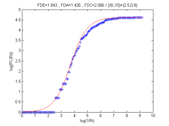
Figure 24: Estimation of the daily arrivals data series FD via parametric sigmoid approximation (red) in the log-log pair-count (blue) plot. The Tukey-weighted $\left(q=0.8\right)$ sigmoid slope at the central point yields FD around 1.84 (“FDE”).

IX Discussion

As it was mentioned from the start, the goal of this study is two-fold: (a) the statistical and signal-level characterization of the smuggling networks as a generating process; and (b) the draft formulation and preliminary assessment of such models for predictive purposes, i.e., to produce short-term forecasting of the refugee influx. Hence, all the results can be explained within this context of system-identification and predictive-analytics capabilities, especially under the scope of changes in policies and mandates that follows the “stable” time frame up to mid-January 2016. Predictive analytics are discussed first, as they provide hints to the statistical properties of the smuggling networks, followed by the system identification of the smuggling networks, as well as some hints for future enhancements and the current state-of-play in the refugee crisis.

IX-A Predictive analytics of the refugee influx

The standard statistics of the refugee influx reveal the nature of the daily arrivals as raw data. More specifically, the first few moments in Table I, as well as the histogram itself in Figure 7, reveal a distinct asymmetry between the left and the right side of the Gaussian approximation. The deviation of mean and median values from the absolute middle of the range confirm the conclusions drawn from the values of kurtosis and skewness, illustrating a trend towards the lower end. In practice, influx rates lower than the mean are a bit more common and more closely packed together than the ones higher than the mean, which are a bit less common and more sparsely distributed (greater variation). These observations are also confirmed by the best-fit parameters of the corresponding Poisson and GEV models.

Based on this statistical profile, it is safe to assert that the distribution is closely approximated by a Gaussian model, which results more or less that it follows the 2/3 inclusion rule for the mean$\pm$stdev range. When weekly-grouped (see: Figure 8), the average daily arrivals reveal a distinct difference in volume between the weekdays, with preference to Sundays and Mondays for the higher influx rates - more than double than the lower influx rates, as Figure 9 shows. Although not very useful for actual short-term forecasting, these data-backed conclusions are a very important verification of qualitative observations conducted throughout the same period by rescue & relief teams in the “hot” zones.

In this study, predictive analytics are described under the scope of various approaches and algorithms, including both daily and weekly-grouped formulations of the raw data. First, the linear and cosine-linear regressions reveal the general trends: a downward linear trend of 47 less arrivals per day within the time frame under investigation; and a primary periodic trend of roughly 6.2-6.5 days, i.e., a repetitive behavioral pattern. The later is further established by examining the largest coefficients of the (simple) linear regressor, where the previous 1-4 & 10-11 days seem to be the most important subset for predicting the next day’s influx rate. This periodic behavior is presented more clearly by the spectral analysis (FFT) in Figure 11 and the frequency-rescaling calculation, where the low-band density profile seems bounded, again, close to the limit of six days or slightly less than a full week.

An actual predictive model with significant short-term forecasting capabilities is the one described by ARMA. Different kernel sizes and adjustments to the time reference used (here, the weekday index) provide very useful insights of how this can be achieved with minimum computational requirements. More specifically, an auto-regressive convolutional kernel using no more than the previous 21 influx spot values can produce a very close approximation to the real data series. Most importantly, analysis of the AR coefficients prove the periodicity of the daily arrivals and the weak correlation between days with a lag 3-4 between them. This essentially confirms the strong correlation between influx rates more than three days apart, or immediately before the current one (lag 1) as in all low-frequency signals, exactly as the previous methods propose too.

The inherent complexity of the daily arrivals data series is characterized quantitatively by the fractal dimension analysis that was described earlier. In practice, a completely deterministic system would present a linear behavior and, therefore, its embedding dimension would be equal to one. On the other hand, a completely stochastic system would present perfectly random fluctuations that would cover its entire plane, i.e., its topological and its embedding dimension would coincide to the value of two (pairs of $\left\{x,y\right\}$ data, where $x$ is the time index and $y$ is the value). In this study, the fractal analysis shows that the (estimated) embedding dimension of the influx data series is 1.84, i.e., somewhere between chaotic and stochastic, closer to the second one. In other words, the daily arrivals show strong non-deterministic properties, but not as much as to make them non-predictable, at least with regard to short-term forecasting.

The weekly-grouped restructuring of the daily arrivals provides an alternative insight to the refugee influx, in terms of weekly patterns and trends. As the results in Figure 17 from SVD analysis show, the daily arrivals is a signal with strong low-frequency signature. According to the histogram of the energy-ranked SVD components, using just the first of them (i.e., associated with the largest eigenvalue) is enough to capture a significant portion of the signal’s energy and, hence, its general shape. In practice, this is not much different than employing an auto-regressive model of order seven (i.e, AR(7)) in the general sense of ARMA, in order to conduct short-term forecasting; but in this case the model’s coefficients are optimized according to its eigenvalues via SVD. As the Figure 17 shows, using the first three or four SVD components, i.e, 3x7=21 or 4x7=28 coefficients is adequate for a close approximation, similarly to the ARMA(21,1,1) that was presented earlier (see: Figure 16). Hence, a three-week time window seems adequate for constructing such analytical models for forecasting purposes in this context.

The K-SVD approach can be used in a similar way, i.e., discover weekly patterns via SVD-based error minimization. However, this assertion is valid only when the corresponding sparsity level is constrained to a very small number, e.g. 1 or 2, at the cost of overall approximation error. On the other hand, using a large dictionary and a large sparsity level can produce a very accurate approximation of the signal, as in Figure 23. This latter approach was the one employed for K-SVD in this study, i.e., to illustrate how such a MF method can be used to design an efficient predictive model for short-term forecasting of the daily arrivals.

IX-B System identification of the smuggling networks

The inherent behavioral properties of the smuggling networks, operating near the Turkish coastline and enabling the travel of thousands of people across the sea passages to the Greek islands, are the underlying statistics of the generating process, i.e., the “system” that creates the daily influx. Normally, this could be formulated more precisely by a full queuing model, including intermediate staging areas or “nodes” inside the mainland and transition routes or “edges” between them, effectively creating a typical network-based framework, e.g. for M/M/1 or M/G/1 analysis (e.g. see: [70]). However, this kind of in-depth analysis requires extensive data series, not only for the daily arrivals influx to Greece, but also for every intermediate “buffer” zone inside Turkey. In other words, the current data sets are sufficient only for a “black box” analysis of this generating process, namely the flow between departures (Turkey) and arrivals (Greece).

As it was mentioned for the predictive analytics, multiple methods point to a very clear periodic trend of roughly 6.2-6.5 days or slightly less than a full week. Linear-cosine regression and spectral analysis (FFT) has shown that the smuggling networks operate more or less in identifiable, almost-weekly behavioral patterns. Additionally, basic statistics and weekly averages show that there is a very distinct difference in daily influx rates between the 48-hour window of Sunday/Monday and the weekdays that follow.These are all clear evidence of a generating process that functions, in total, as a store-and-forward “black box”. It is known that the smuggling networks operating inside Turkey can actually be viewed as flow graphs, very similar to the data networks that employ buffers and store-and-forward techniques as part of their routing protocols (e.g. see: [70]). As described earlier, lack of detailed data for the internals of these smuggling networks effectively means that they can only be studied from the “outside”, i.e., with regard to their total “throughput”. Nevertheless, this evidence almost certainly proves that they operate in a (almost) two-day “burst” / five-day “pause” pattern, an assertion that complies completely with the results from the ARMA modeling.

The PPCA and ICA approaches are alternatives to the MF analysis of the weekly-grouped daily arrivals, not based on eigenvectors as in SVD but employing decorrelation and independency as the statistical constraints for the components, accordingly. In both cases, the blind “discovery” (in the BSS sense) of the underlying components or statistical “sources” that characterize the generating process is indeed a very effective investigation on how the smuggling networks. More specifically, the dominating weekly patterns, illustrated in Figure 18 for PPCA and in Figure 19 for ICA, as well as their relative energy distribution (for ICA, see: Figure 20), show that not only the signal is a low-frequency data series but the high influx rates are mostly associated to the Sunday/Monday 48-hour time frame.

IX-C Recent changes and retrospective

After a long period of discussions and meetings that had started as early as mid-November 2015, on March 18-20th 2016 the EU summit finalized and concluded the deal with Turkey regarding the handling of refugee flows from its coasts to the Greek islands. The mutual agreement included: (a) Turkey’s commitment in stopping the smuggling networks to drastically reduce the refugee influx towards Greece, (b) the involvement of NATO naval forces (SNMG2) for intensifying the monitoring of the most commonly used sea passages and (c) the immediate registering and deportation back to Turkey of any refugees landing in Greece, with the intent of either granting them passage to Europe via air travel (if recognized as “in danger”) or sending them back to their countries of origin.

This new EU-Turkey deal had very significant and almost immediate effects to the refugee influx in the Greek islands of first reception, where hundreds of thousands of people had arrived during the previous months. Figure 25 is an extension of the data series used throughout this study, as presented in Figure 5, including two special periods in 2016: (a) mid-February to March 20th and (b) March 20th to mid-April and current status. It is clear that the plot of the first one presents a pattern very similar to the previous period, i.e., the one analyzed thoroughly in this study, only now the time scale seems “compressed”: Indeed, there are nine peaks in the daily arrivals within a month, when the same pattern would have taken about 50 days if projected to an earlier time - a shrinking factor of about 50/30 or 1.67 (rough estimation, based on the plots). This can be easily explained by the urgency of the smuggling networks to “push” any remaining refugee “packets”, as fast as possible, before the EU-Turkey deal was concluded and much stricter restrictions would be enforced in the sea passages. With regard to the period after the March 20th, when the deal was in place and active, it should be noted that UNHCR and other NGOs that were involved in the reception and registration of the refugees in Greece’s “hotspots” decided to terminate their presence there, stating that this deal is violating fundamental human rights and the UN Convention about refugees and asylum seekers. As a result, registration of any daily arrivals (significantly reduced but certainly non-zero) is being conducted exclusively by the Greek authorities and, hence, there are no relevant data publicly accessible, as there was the case up to this date. Practically, this means that (a) is a very different data series in terms of statistical properties compared to the data set used in this study, while (b) is considered as missing/incomplete data time frame. These limitations were the main reason for setting the maximum usable “valid” date for this study at mid-January 2016, even though more data were available.

Figure 25: Estimated daily arrivals and weekly averages for the entire Greece, including the weeks just before and after the EU-Turkey deal (Feb-Apr.2016).

Another, more important outcome from the recent EU-Turkey deal and the strict controls imposed on the sea passages towards the Greek islands is the gradual shift of the refugee influx to the Central Med. route. Figure 26 illustrates the comparison between daily arrivals to Greece and to Italy during the weeks just before and after the deal. Although not quantified and analyzed here, it is evident that there is a strong negative correlation between the two data series: up to March 15th, the arrivals to Italy were practically zero, while Greece was receiving the last large “packets” before the activation of the new regime; from there on, there is a mixture of influx rates in both countries, in reduced rates; in the week following the mark of March 20th, the influx rates are very limited even for Greece; and finally, by the end of March there is a very large peak of refugee influx to Italy, almost 10 times the one registered towards Greece (2,691/281=9.57).

Figure 26: Comparison of refugee influx in Greece and Italy just before and after the EU-Turkey deal (Mar-Apr.2016).

The same pattern continues well within April, according to more recent data from IOM and UNHCR (not presented here). It seems that the new EU-Turkey deal does not actually stop the refugee influx towards Europe, only shifts it to previous, more dangerous routes, as it was the case 18-24 months earlier when the Mare Nostrum operation (Italy) was in place in the Central Med. route - only now, the Triton operation (EU/Frontex) is much more limited in scope and the total refugee influx is multiplied many times more. It is clear that, as long as the conditions remain the same and the war zones in Syria, Iraq, Afghanistan and elsewhere force people out and away from their homes, refugees will continue to converge towards Europe via the Mediterranean Sea. Therefore, the need for such early warning/alerting systems will continue to be an imperative need in Greece, in Italy or elsewhere.

IX-D Future work

The current study focused entirely in the daily arrivals of the refugees, i.e., on the influx data series. The goal was to conduct a data-driven analysis and modeling based on this data set alone. However, it is established that the intensity of the daily arrivals at the Greek islands is strongly associated to specific external factors, such as weather conditions, changes in refugee handling policies by the EU, the intensity of fights in the war zones in Syria, etc. Some of these factors can be quantified and included in such data-driven approaches, others can not.

The most promising external factor that may be used as “input” in these models is weather conditions. More specifically, it was pointed out empirically from early on that some weather elements are of utmost importance, such as wind intensity and wave height (not always correlated), while others were of lesser importance, such as rainfall, temperature, humidity or cloud coverage. Hence, wind intensity and wave height are the two external factors that will be investigated subsequently, in correlation to the core influx data series, in order to establish the significance of the statistical relevance and use these as additional inputs in the predictive analytics.

The issue of localization is also a factor that may be considered in more detail. In this study, only the total influx was used as a single data series; however, if more data are available or in cases where the local influx rates are sufficiently high for statistical significance (e.g. in Lesvos), localized data analysis and predictive modeling may be conducted. Combined with localized weather information, such systems would be even more useful and preemptive life-saving tools in the field of SSAR operations.

In terms of an actual early warning/alerting module for integration into rescue and relief operations, especially in “hot” zones like in eastern Greece and southern Italy, these predictive analytics have to be reformulated more strictly, assessed in terms of true performance on unknown data (k-fold cross validation testing [20]) and finalized with specific “alert levels” as output accordingly, similar to the way such systems of Civil Protection agencies work in other contexts, e.g. for tsunamis, wildfires, floods, etc. Ideally, this module could be fed with live data from registration agencies and other open data sources, publicly available Internet sources and satellite feeds, in order to produce reliable real-time short-term early warning of possible 24/48-hour influx periods of high intensity. This is already investigated as an add-in feature in “Prometheus”, a virtual Emergency Operations Center (EOC) developed and deployed already in Chios since January 2016 [71, 72].

X Conclusions

This study presents the first-ever data-driven systemic analysis of systemic analysis of the refugee influx in Greece, aiming at: (a) the statistical and signal-level characterization of the smuggling networks and (b) the formulation and preliminary assessment of such models for predictive purposes, i.e., as the basis of such an early warning/alerting protocol for the rescue and relief operations on-site.

The analysis employed a wide range of statistical, signal-based and matrix factorization (decomposition) techniques. It was established that the behavioral patterns of the smuggling networks closely match (as expected) the regular “burst” and “pause” periods of store-and-forward networks in digital communications. The most interesting aspect is the discovery of a strong almost-weekly periodic trend of 6.2-6.5 days, as well as a strong preference of the Sunday/Monday 48-hour time window for the highest peaks of influx rates.

These results show that such models can be used successfully for short-term forecasting of the influx intensity, producing an invaluable operational asset for planners, decision-makers and first-responders. It is expected that future extensions of these models, including weather factors (wind intensity, wave height) will further increase their accuracy and their value as actual early warning tools in such operations.

Harris Georgiou received his B.Sc. degree in Informatics from University of Ioannina, Greece, in 1997, and his M.Sc. degree in Digital Signal Processing & Computer Systems and Ph.D. degree in Machine Learning & Medical Imaging, from National & Kapodistrian University of Athens, Greece, in 2000 and 2009, respectively. Since 1998, he has been working with the Signal & Image Processing Lab (SIPL) in the Department of Informatics & Telecommunications (DIT) at National & Kapodistrian University of Athens (NKUA/UoA), Greece, in various academic and research projects. In 2013-2015 he worked as a post-doctorate associate researcher with SIPL in sparse models for distributed analysis of functional MRI (fMRI) signals. He has been actively involved in several national and EU-funded research & development projects, focusing on new and emerging technologies in Biomedicine and applications. He has also worked in the private sector as a consultant in Software Engineering and Quality Assurance (SQA, EDP/IT), as well as a faculty professor in private institutions in various ICT-related subjects, for more than 18 years. His main research interests include Machine Learning, Pattern Recognition, Signal Processing, Medical Imaging, Soft Computing, Artificial Intelligence and Game Theory. He has published more than 71 papers and articles (46 peer-reviewed) in various academic journals & conferences, open-access publications and scientific magazines, as well as two books in Biomedical Engineering & Computer-Aided Diagnosis and several contributions in seminal academic textbooks in Machine Learning & Pattern Recognition. He is a member of the IEEE and the ACM organizations, general secretary in the A.C. board of the Hellenic Informatics Union (HIU), team coordinator of the Greek ICT4D task group & the “Sahana4Greece” (virtual EOC for the refugee crisis) initiative and he has given several technical presentations in various countries.

References

- [1] UNHCR, “Unhcr: Mediterranean sea arrivals – 2015 data by location, country of arrival (data).” [Online]. Available: http://data.unhcr.org/mediterranean/download.php?id=490
- [2] IOM, “Iom: Missing migrants project - mediterranean, update 12 april 2016.” [Online]. Available: http://migration.iom.int/Europe/
- [3] MSF, “Msf: Obstacle course to europe (report).” [Online]. Available: http://www.msf.gr/publications/obstacle-course-europe
- [4] UNHCR, “Unhcr: Daily estimated arrivals per country – flows through western balkans route (portal).” [Online]. Available: http://data.unhcr.org/mediterranean/regional.php
- [5] HCG, “Hellenic coast guard - statistics of operations (2015).” [Online]. Available: http://www.hcg.gr
- [6] TCGC, “Turkish coast guard command - statistics of operations (2015).” [Online]. Available: http://www.sgk.tsk.tr/
- [7] IOM, “(iom) analysis: Flow monitoring surveys - mediterranean, data collected: 8 oct 2015 - 4 apr 2016.” [Online]. Available: http://is.gd/iZrIII
- [8] BBC, “(bbc) migrant crisis: Hundreds dead after capsize, say survivors - 18 apr 2016.” [Online]. Available: http://www.bbc.com/news/world-africa-36071737
- [9] Wikipedia, “2013 lampedusa migrant shipwreck.” [Online]. Available: https://en.wikipedia.org/wiki/2013_Lampedusa_migrant_shipwreck
- [10] T. Telegraph, “(the telegraph) un confirms 800 dead in shipwreck disaster: as it happened on april 20.” [Online]. Available: http://is.gd/iukThZ
- [11] Wikipedia, “Operation mare nostrum (italy).” [Online]. Available: https://en.wikipedia.org/wiki/Operation_Mare_Nostrum
- [12] ——, “Operation triton (eu frontex).” [Online]. Available: https://en.wikipedia.org/wiki/Operation_Triton
- [13] N. Times, “European union reaches deal with turkey to return new asylum seekers.” [Online]. Available: http://is.gd/9gOyVx
- [14] UNHCR, “Unhcr: Daily estimates per location 29 oct 2015 – 20 jan 2016 (report).” [Online]. Available: http://data.unhcr.org/mediterranean/download.php?id=456
- [15] ——, “Unhcr: Daily estimates per location 29 oct 2015 – 20 jan 2016 (data).” [Online]. Available: http://data.unhcr.org/mediterranean/download.php?id=456
- [16] MathWorks, “Mathworks matlab (r2015b).” [Online]. Available: http://www.mathworks.com/products/matlab/
- [17] U. o. W. Machine Learning Group, “Weka (v3.7.13).” [Online]. Available: http://www.cs.waikato.ac.nz/~ml/weka/
- [18] M. Spiegel, J. Schiller, and R. Srinivasan, Probability and Statistics (3rd/Ed.). McGraw-Hill: 2009, 2009.
- [19] M. Spiegel, J. Liu, and S. Lipschutz, Mathematical Handbook of Formulas and Tables (4th/Ed.). McGraw-Hill: 2012, 2012.
- [20] S. Theodoridis and K. Koutroumbas, Pattern Recognition, Fourth Edition. Academic Press, 2009.
- [21] S. Kotz and S. Nadarajah. Imperial College Press, London (UK).
- [22] E. Hannan, “The estimation of the order of an arma process,” Ann. Statistics, vol. 5, pp. 170–181, 1993.
- [23] A. Oppenheim and R. Schafer, Digital Signal Processing. Prentice-Hall: 1975, 1975.
- [24] D. Manolakis and J. Proakis, Introduction to Digital Signal Processing. Macmillan: 1989, 1989.
- [25] C. Therrien, Discrete Random Signals and Statistical Signal Processing. Prentice-Hall: 1992, 1992.
- [26] F. J. Harris, “On the use of windows for harmonic analysis with the discrete fourier transform,” Proc.IEEE., vol. 66, pp. 66–67, 1978.
- [27] H. Hsu, Signals and Systems. McGraw-Hill: 1995, 1995.
- [28] A. Oppenheim, A. Willsky, and I. Young, Signals and Systems. Prentice-Hall: 1983, 1983.
- [29] R. Hamming, Digital Filters, 3rd/Ed. Dover Publications: 1989, 1989.
- [30] B. Porat, Digital Processing of Random Signals - Theory and Methods. Dover Publications: 1994, 1994.
- [31] M. Elad, Sparse and Redundant Representations: From Theory to Applications in Signal and Image Processing. Springer, 2010.
- [32] G. I. Allen, “SVD on high dimensions,” Tech. Rep.
- [33] M. Tipping and C. Bishop, “Probabilistic principal component analysis,” Journal of the Royal Statistical Society - Series B (Statistical Methodology), vol. 61, no. 3, pp. 611–622, 1999.
- [34] D. R. Langers, “Blind source separation of fMRI data by means of factor analytic transformations,” NeuroImage, vol. 47, no. 1, pp. 77–87, Aug. 2009. [Online]. Available: http://www.sciencedirect.com/science/article/pii/S1053811909003681
- [35] J. Bobin, J.-L. Starck, Y. Moudden, and M. J. Fadili, “Blind source separation: the sparsity revolution,” Advances in Imaging and Electron Physics, vol. 152, pp. 221–302, 2008. [Online]. Available: http://www.sciencedirect.com/science/article/pii/S1076567008006058
- [36] V. Abolghasemi, S. Ferdowsi, and S. Sanei, “Blind separation of image sources via adaptive dictionary learning,” IEEE Transactions on Image Processing, vol. 21, no. 6, pp. 2921–2930, Jun. 2012. [Online]. Available: http://ieeexplore.ieee.org/lpdocs/epic03/wrapper.htm?arnumber=6151824
- [37] J. Silva, M. Chen, Y. C. Eldar, G. Sapiro, and L. Carin, “Blind compressed sensing over a structured union of subspaces,” arXiv preprint arXiv:1103.2469, 2011. [Online]. Available: http://arxiv.org/abs/1103.2469
- [38] A. Hyvarinen, J. Karhunen, and E. Oja, Independent Component Analysis. Wiley-Interscience, 2001.
- [39] A. Hyvärinen and E. Oja, “Independent component analysis: algorithms and applications,” Neural Networks, vol. 13, pp. 411–430, 2000.
- [40] P. Bai, H. Shen, and Y. Truong, “Robust independent component analysis for fMRI,” 2006. [Online]. Available: http://sisla06.samsi.info/ranmat/rc/ranmat-rc/Truong_main.pdf
- [41] M. Behroozi, M. R. Daliri, and H. Boyaci, “Statistical analysis methods for the fmri data,” Basic and Clinical Neuroscience, vol. 2, no. 4, pp. 67–74, 2011.
- [42] V. D. Calhoun, T. Adali, J. Hansen, L. K.and Larsen, and J. J. Pekar, “Ica of functional mri data: An overview,” in Proc. Int. Symp. Indep. Comp. Analysis (ICA 2003).
- [43] V. D. Calhoun and T. Adali, “Unmixing fMRI with independent component analysis,” Engineering in Medicine and Biology Magazine, IEEE, vol. 25, no. 2, pp. 79–90, 2006. [Online]. Available: http://ieeexplore.ieee.org/xpls/abs_all.jsp?arnumber=1607672
- [44] A. Hyvärinen and E. Oja, “Fastica toolbox for matlab.” [Online]. Available: http://research.ics.aalto.fi/ica/fastica/index.shtml
- [45] ——, “A fast fixed-point algorithm for independent component analysis,” Neural Computation, vol. 9, no. 7, pp. 1483–1492, 1997.
- [46] A. Hyvärinen, “Fast and robust fixed-point algorithms for independent component analysis,” Neural Networks, vol. 10, pp. 626–634, 1999.
- [47] N. Correa, T. Adali, Y.-O. Li, and V. Calhoun, “Comparison of blind source separation algorithms for fmri using a new matlab toolbox: Gift,” in Acoustics, Speech, and Signal Processing, 2005. Proceedings. (ICASSP ’05). IEEE International Conference on, vol. 5, March 2005, pp. v/401–v/404 Vol. 5.
- [48] I. Tosic and P. Frossard, “Dictionary learning,” IEEE Signal Processing Magazine, vol. 28, no. 2, pp. 27 –38, Mar. 2011.
- [49] H. Lee, A. Battle, R. Raina, and A. Ng, “Efficient sparse coding algorithms,” in Advances in neural information processing systems, 2006, pp. 801–808. [Online]. Available: http://machinelearning.wustl.edu/mlpapers/paper_files/NIPS2006_878.pdf
- [50] T. S., K. Y., and S. K., Sparsity-Aware Learning and Compressed Sensing: An Overview. Academic Press, 2014.
- [51] V. Abolghasemi, S. Ferdowsi, and S. Sanei, “Fast and incoherent dictionary learning algorithms with application to fMRI,” Signal, Image and Video Processing, Feb. 2013. [Online]. Available: http://link.springer.com/10.1007/s11760-013-0429-2
- [52] Y. Kopsinis, H. Georgiou, and S. Theodoridis, “fmri unmixing via properly adjusted dictionary learning,” in 22th European Signal Processing Conference (EUSIPCO 2014).
- [53] T. Bai, Y. F. Li, and X. Zhou, “Robust and fast visual tracking using constrained sparse coding and dictionary learning,” in Intelligent Robots and Systems (IROS), 2012 IEEE/RSJ International Conference on, 2012, pp. 3824–3829. [Online]. Available: http://ieeexplore.ieee.org/xpls/abs_all.jsp?arnumber=6385459
- [54] M. G. Jafari and M. D. Plumbley, “Speech denoising based on a greedy adaptive dictionary algorithm,” in Proc. European Signal Processing Conf, 2009. [Online]. Available: http://www.eurasip.org/Proceedings/Eusipco/Eusipco2009/contents/papers/1569192606.pdf
- [55] R. Rubinstein, M. Zibulevsky, and M. Elad, “Efficient implementation of the k-SVD algorithm using batch orthogonal matching pursuit,” CS Technion, 2008. [Online]. Available: http://pdf.aminer.org/000/322/616/efficient_computation_for_sequential_forward_observation_selection_in_image_reconstruction.pdf
- [56] M. Aharon, M. Elad, and A. Bruckstein, “K-SVD: an algorithm for designing overcomplete dictionaries for sparse representation,” IEEE Transactions on Signal Processing, vol. 54, no. 11, pp. 4311–4322, Nov. 2006. [Online]. Available: http://ieeexplore.ieee.org/lpdocs/epic03/wrapper.htm?arnumber=1710377
- [57] K. Lee and J. C. Ye, “A data-driven fmri analysis using k-svd sparse dictionary learning,” International Society of Magnetic Resonance in medicine (ISMRM), 2010.
- [58] R. Rubinstein, T. Faktor, and M. Elad, “K-SVD dictionary-learning for the analysis sparse model,” in 2012 IEEE International Conference on Acoustics, Speech and Signal Processing (ICASSP), Mar. 2012, pp. 5405 –5408.
- [59] K. Skretting and K. Engan, “Recursive least squares dictionary learning algorithm,” IEEE Transactions on Signal Processing, vol. 58, no. 4, pp. 2121–2130, Apr. 2010. [Online]. Available: http://ieeexplore.ieee.org/lpdocs/epic03/wrapper.htm?arnumber=5382523
- [60] C. Boutsidis and P. Drineas, “Random projections for the nonnegative least-squares problem,” Linear Algebra and its Applications, vol. 431, no. 5-7, pp. 760–771, 2009.
- [61] C.-J. Lin, “Projected gradient methods for nonnegative matrix factorization,” Neural Computation, vol. 19, no. 10, pp. 2756–2779, 2007.
- [62] T. Adah, M. Anderson, and G. Fu, “IVA and ICA: use of diversity in independent decompositions,” in Signal Processing Conference (EUSIPCO), 2012 Proceedings of the 20th European, 2012, pp. 61–65. [Online]. Available: http://ieeexplore.ieee.org/xpls/abs_all.jsp?arnumber=6334326
- [63] J. L. Encarnacao, H.-O. Peitgen, G. Sakas, and G. E. Englert, Fractal Geometry and Computer Graphics. Springer-Verlag, Berlin, 1992.
- [64] P. R. Massopust, Fractal Functions, Fractal Surfaces and Wavelets. Academic Press, San Diego, 1994.
- [65] C. C. Chen, J. S. Daponte, and F. M. D., “Fractal feature analysis and classification in medical imaging,” IEEE Trans. Med. Im., vol. 8, no. 2, pp. 133–142, 1989.
- [66] A. W. Moore and M. S. Lee, “Efficient algorithm for minimizing cross validation error,” in Proceedings of the 11th.International Conference on Machine Learning (ML-94), 10-13 July 1994, New Brunswick, New Jersey.
- [67] S. Pierre and J. F. Rivest, “On the validity of fractal dimension measurements in image analysis,” J. Vis. Com. Im. Proc., vol. 7, no. 3, pp. 217–229, 1996.
- [68] C. J. Traina, A. J. Traina, L. Wu, and C. Faloutsos, “Fast feature selection using fractal dimension,” in XV Brazilian Database Symposium 2000, Joao Pessoa, PA Brazil.
- [69] B. Abrahao and L. Barbosa, “Characterizing datasets using fractal methods,” Dept. of Computer Science, Universidade Federal de Minas Gerais, Belo Horizonte, MG Brazil, 2003.
- [70] D. Bertsekas and R. Gallager, Data Networks (2nd/Ed.). Prentice Hall: 1992, 1992.
- [71] S. Anastasiadis and H. Georgiou, “Prometheus: The virtual Emergency Operations Center for Chios and refugee influx data analytics,” in Free and Open-Source Software Communities (FOSSCOMM 2016), 2016.
- [72] S. Anastasiadis, “Prometheus: The virtual Emergency Operations Center for Chios.” [Online]. Available: http://chios.prometheus.online