A probabilistic max-plus numerical method for solving stochastic control problems

Abstract

We consider fully nonlinear Hamilton-Jacobi-Bellman equations associated to diffusion control problems involving a finite set-valued (or switching) control and possibly a continuum-valued control. We construct a lower complexity probabilistic numerical algorithm by combining the idempotent expansion properties obtained by McEneaney, Kaise and Han (2011) for solving such problems with a numerical probabilistic method such as the one proposed by Fahim, Touzi and Warin (2011) for solving some fully nonlinear parabolic partial differential equations. Numerical tests on a small example of pricing and hedging an option are presented.

I Introduction

We consider a finite horizon diffusion control problem on $\mathbb{R}^{d}$ involving at the same time a “discrete” control taking its values in a finite set $\mathcal{M}$, and a “continuum” control taking its values in some subset $\mathcal{U}$ of a finite dimensional space $\mathbb{R}^{p}$ (for instance a convex set with nonempty interior), which we next describe.

Let $T$ be the horizon. The state $\xi_{s}\in\mathbb{R}^{d}$ at time $s\in[0,T]$ satisfies the stochastic differential equation

$$d\xi_{s}=f^{\mu_{s}}(\xi_{s},u_{s})ds+\sigma^{\mu_{s}}(\xi_{s},u_{s})dW_{s}\enspace,$$ (1)

where $(W_{s})_{s\geq 0}$ is a $d$-dimensional Brownian motion on a filtered probability space $(\Omega,\mathcal{F},(\mathcal{F}_{s})_{0\leq s\leq T},P)$. The control processes $\mu:=(\mu_{s})_{0\leq s\leq T}$ and $u:=(u_{s})_{0\leq s\leq T}$ take their values in the sets $\mathcal{M}$ and $\mathcal{U}$ respectively and they are admissible if they are progressively measurable with respect to the filtration $(\mathcal{F}_{s})_{0\leq s\leq T}$. We assume that, for all $m\in\mathcal{M}$, the maps $f^{m}:\mathbb{R}^{d}\times\mathcal{U}\to\mathbb{R}^{d}$ and $\sigma^{m}:\mathbb{R}^{d}\times\mathcal{U}\to\mathbb{R}^{d\times d}$ are continuous and satisfy properties implying the existence of the process $(\xi_{s})_{0\leq s\leq T}$ for any admissible control processes $\mu$ and $u$.

Given an initial time $t\in[0,T]$, the control problem consists in maximizing the following payoff:

$$J(t,x,\mu,u):=\mathbb{E}\left[\int_{t}^{T}e^{-\int_{t}^{s}\delta^{\mu_{\tau}}(\xi_{\tau},u_{\tau})d{\tau}}\ell^{\mu_{s}}(\xi_{s},u_{s})ds\right.$$

$$\left.\quad+e^{-\int_{t}^{T}\delta^{\mu_{\tau}}(\xi_{\tau},u_{\tau})d{\tau}}\psi(\xi_{T})\mid\xi_{t}=x\right]\enspace,$$

where, for all $m\in\mathcal{M}$, $\ell^{m}:\mathbb{R}^{d}\times\mathcal{U}\to\mathbb{R}$, $\delta^{m}:\mathbb{R}^{d}\times\mathcal{U}\to\mathbb{R}_{+}$ (the set of positive reals), and $\psi:\mathbb{R}^{d}\to\mathbb{R}$ are given continuous maps. We then define the value function of the problem as the optimal payoff:

$$v(t,x)=\sup_{\mu,u}J(t,x,\mu,u)\enspace,$$

where the maximization holds over all admissible control processes $\mu$ and $u$.

Let $\mathbb{S}_{d}$ denotes the set of symmetric $d\times d$ matrices. The Hamiltonian $\mathcal{H}:\mathbb{R}^{d}\times\mathbb{R}\times\mathbb{R}^{d}\times\mathbb{S}_{d}\to\mathbb{R}$ of the above control problem is defined as:

$$\mathcal{H}(x,r,p,\Gamma):=\max_{m\in\mathcal{M}}\mathcal{H}^{m}(x,r,p,\Gamma)\enspace,$$

with

$$\mathcal{H}^{m}(x,r,p,\Gamma):= \max_{u\in\mathcal{U}}\Big{\{}\frac{1}{2}\mathop{\mathrm{tr}}\left(\sigma^{m}(x,u)\sigma^{m}(x,u)^{\mathsf{T}}\,\Gamma\right)$$

$$+f^{m}(x,u)\cdot p-\delta^{m}(x,u)r+\ell^{m}(x,u)\Big{\}}\enspace.$$

Under suitable assumptions, the value function $v:[0,T]\times\mathbb{R}^{d}\to\mathbb{R}$ is the unique (continuous) viscosity solution of the following Hamilton-Jacobi-Bellman equation

$$-\frac{\partial v}{\partial t}-\mathcal{H}(x,v(t,x),Dv(t,x),D^{2}v(t,x))=0,$$ (2)

$$\;\hskip 100.00015ptx\in\mathbb{R}^{d},\;t\in[0,T),$$

$$v(T,x)=\psi(x),\quad x\in\mathbb{R}^{d},$$

satisfying also some growth condition at infinity (in space).

In [1], Fahim, Touzi and Warin proposed a probabilistic numerical method to solve such fully nonlinear partial differential equations (2), inspired by their backward stochastic differential equation interpretation given by Cheridito, Soner, Touzi and Victoir in [2]. However this method only works when the diffusion matrices $\sigma^{m}(x,u)\sigma^{m}(x,u)^{\mathsf{T}}\,$ are at the same time bounded from below (with respect to the Loewner order) by a symmetrix positive definite matrix $a$ and bounded from above by $(1+2/d)a$. Such a constraint can be restrictive, in particular it may not hold even when the matrices $\sigma^{m}(x,u)$ do not depend on $x$ and $u$ but take different values for $m\in\mathcal{M}$. Also some regularity conditions may be needed for $\mathcal{H}$, which are not fulfilled when $\mathcal{M}$ is a finite set.

McEneaney, Kaise and Han proposed in [3, 4] an idempotent numerical method which works at least when the hamiltonian $\mathcal{H}^{m}$ corresponds to linear quadratic control problems. This method is based on the distributivity of the (usual) addition operation over the supremum (or infimum) operation, and on a property of invariance of the set of quadratic forms. It computes in a backward manner the value function $v(t,\cdot)$ at time $t$ as a supremum of quadratic forms. However, as $t$ decreases, the number of quadratic forms generated by the method increases exponentially (and even become infinite if the Brownian is not discretized in space) and some pruning is necessary to reduce the complexity of the algorithm.

Here, we combine the two above methods to construct a new algorithm. The method is using in particular the simulation of a small number of uncontrolled stochastic processes as in [1]. We show that even without pruning, the complexity of the algorithm is bounded polynomially in the number of discretization time steps and in the size of the sample of the uncontrolled stochastic processes. Numerical tests of our algorithm on an example of pricing and hedging an option in dimension 2 considered in [5] are presented.

II The algorithm of Fahim, Touzi and Warin

Let $h$ be a time discretization step such that $T/h$ is an integer. We denote by $\mathcal{T}_{h}=\{0,h,2h,\ldots,T-h\}$ the set of discretization times of $[0,T)$.

For each $m\in\mathcal{M}$, we shall assume that we can apply the algorithm of [1] to the equation:

$$-\frac{\partial v}{\partial t}-\mathcal{H}^{m}(x,v(t,x),Dv(t,x),D^{2}v(t,x))=0,$$ (3)

$$\;\hskip 100.00015ptx\in\mathbb{R}^{d},\;t\in[0,T).$$

For this purpose, we decompose $\mathcal{H}^{m}$ as the sum of the (linear) generator $\mathcal{L}^{m}$ of a diffusion (with no control) and of a nonlinear elliptic Hamiltonian $\mathcal{G}^{m}$, that is $\mathcal{H}^{m}=\mathcal{L}^{m}+\mathcal{G}^{m}$ with

$$\mathcal{L}^{m}(x,r,p,\Gamma):= \frac{1}{2}\mathop{\mathrm{tr}}\left(a^{m}(x)\Gamma\right)+\underline{f}^{m}(x)\cdot p\enspace,$$

$a^{m}(x)=\underline{\sigma}^{m}(x)\underline{\sigma}^{m}(x)^{\mathsf{T}}\,$ and $\mathcal{G}^{m}$ such that $\partial_{\Gamma}{\mathcal{G}^{m}}$ is positive semidefinite, for all $x\in\mathbb{R}^{d},\;r\in\mathbb{R},p\in\mathbb{R}^{d},\Gamma\in\mathbb{S}_{d}$. We also assume that $\mathop{\mathrm{tr}}(a^{m}(x)^{-1}\partial_{\Gamma}{\mathcal{G}^{m}})\leq 1$.

The time discretization of (3) proposed in [1] can be written in the following form:

$$v^{h}(t,x)=T_{t,h}^{m}(v^{h}(t+h,\cdot))(x),\quad t\in\mathcal{T}_{h}\enspace,$$

where, under some conditions, $T_{t,h}^{m}$ is a monotone operator over the set of Lipschitz continuous functions from $\mathbb{R}^{d}$ to $\mathbb{R}$:

$$\phi\leq\psi\implies T_{t,h}^{m}(\phi)\leq T_{t,h}^{m}(\psi)\enspace.$$ (4)

Moreover, the operator $T_{t,h}^{m}$ is constructed by using a probabilistic scheme. Denote by $\hat{X}^{m}$ the Euler discretization of the diffusion with generator $\mathcal{L}^{m}$:

$$\hat{X}^{m}(t+h)=$$ (5)

$$\hat{X}^{m}(t)+\underline{f}^{m}(\hat{X}^{m}(t))h+\underline{\sigma}^{m}(\hat{X}^{m}(t))(W_{t+h}-W_{t})\enspace.$$

Then,

$$T_{t,h}^{m}(\phi)(x)=\mathcal{D}_{m,t,h}^{0}(\phi)(x)$$ (6)

$$+h\mathcal{G}^{m}(x,\mathcal{D}_{m,t,h}^{0}(\phi)(x),\mathcal{D}_{m,t,h}^{1}(\phi)(x),\mathcal{D}_{m,t,h}^{2}(\phi)(x))$$

with, for $i=0,1,2$, $\mathcal{D}_{m,t,h}^{i}(\phi)$ being the approximation of the $i$th derivative of $\phi$ obtained as follows:

$$\mathcal{D}_{m,t,h}^{i}(\phi)(x)=\mathbb{E}(\phi(\hat{X}^{m}(t+h))\mathcal{P}^{i}_{m,t,x,h}(W_{t+h}-W_{t})\mid\hat{X}^{m}(t)=x)\enspace,$$

where, for all $m,t,x,h,i$, $\mathcal{P}^{i}_{m,t,x,h}$ is a polynomial of degree $i$ with values in an appropriate finite dimensional space, and in particular $\mathcal{P}^{0}_{m,t,x,h}\equiv 1$. Although the operator $T_{t,h}^{m}$ does not depend on $t$, since both the law of $W_{t+h}-W_{t}$ and the Hamiltonian $\mathcal{H}^{m}$ do not depend on $t$, we keep the index $t$ since it will become important when applying a regression approximation (see below).

In [1], the convergence of such a time discretization is proved under the above assumptions and some other technical assumptions. Note that these conditions include the boundedness of the coefficients of the Hamiltonians $\mathcal{L}^{m}$ and $\mathcal{H}^{m}$, and the boundedness of the value function of the corresponding control problem. However, a change of variable on the value and on the state allows one to obtain the same type of result for unbounded coefficients and value function satisfying some suitable growth conditions at infinity. Such a change of variables may induce a deformation on the discretizations (5) and (6) and so on the algorithm, but we shall not discuss this here. A greater difficulty is that the above assumptions do not allow in general to handle directly the case where $\mathcal{H}^{m}$ is replaced by $\mathcal{H}$. However, in the case of $\mathcal{H}$ as above one can simply consider the following scheme:

$$v^{h}(t,x)=\max_{m\in\mathcal{M}}\{T_{t,h}^{m}(v^{h}(t+h,\cdot))(x)\},\quad t\in\mathcal{T}_{h}\enspace.$$ (7)

The difference with the usual scheme of [1] is that one needs to construct several operators $T_{t,h}^{m}$ and so several processes $\hat{X}^{m}$, one for each $m\in\mathcal{M}$. The solution $v^{h}$ of this time discretization will converge to the value function of our problem, that is the solution of the Hamilton-Jacobi-Bellman equation with hamiltonian $\mathcal{H}$, as soon as the convergence is proved for the time discretization of the equations with hamiltonians $\mathcal{H}^{m}$.

Although the above scheme can be compared to a standard numerical approximation if one develops the expression of each $T_{t,h}^{m}(\phi)(x)$, with $m\in\mathcal{M}$, one may compute $v^{h}$ given by (7) as in [1], that is using a regression estimator. One just simulates the process $\hat{X}^{m}$ and do at each time $t\in\mathcal{T}_{h}$ a regression estimation to find the value of $\mathcal{D}_{m,t,h}^{i}(v^{h}(t+h,\cdot))$ at the points $\hat{X}^{m}(t)$ by using the values of $\hat{X}^{m}(t+h)$ and $W_{t+h}-W_{t}$.

Although this variation of the method of [1], based on (7), is appealing and may work in practice, several difficulties remain. First, theoretically, the sample size to obtain the convergence of the estimator is at least in the order of $1/h^{d/2}$ [6]. Hence, it is exponential in the dimension of the system showing the persistence of the curse of dimensionality, although in some practical examples, a much smaller sample size may be sufficient. Next, one possible regression estimation is to approximate the conditional expectation of a random map by projecting it orthogonally into a finite dimensional linear space of functions. Then, to obtain a good estimation, the dimension of this space need to be exponential in the dimension $d$. In the sequel, we shall rather use a small dimensional regression space and use a distributivity property as in the work of McEneaney, Kaise and Han [3, 4] to find a good approximation of $v_{h}$ living in the max-plus linear space of finite suprema of quadratic forms.

III The algorithm of McEneaney, Kaise and Han

In [3, 4], the following time discretization is used. Denote by $\hat{\xi}^{m,u}$ the Euler discretization of the process $\xi$ defined in the introduction, when the controls $m$ and $u$ are fixed:

$$\hat{\xi}^{m,u}(t+h)= \hat{\xi}^{m,u}(t)+f^{m}(\hat{\xi}^{m,u}(t),u)h+$$

$$\qquad\sigma^{m}(\hat{\xi}^{m,u}(t),u)(W_{t+h}-W_{t})\enspace.$$

Then, a time discretization of the solution of (2) is given by:

$$v^{h}(t,x)=T_{t,h}(v^{h}(t+h,\cdot))(x),\quad t\in\mathcal{T}_{h}\enspace,$$ (8)

where

$$T_{t,h}(\phi)(x)= \sup_{m\in\mathcal{M},u\in\mathcal{U}}\Big{\{}h\ell^{m}(x,u)+e^{-h\delta^{m}(x,u)}$$

$$\qquad\qquad\mathbb{E}\big{[}\phi(\hat{\xi}^{m,u}(t+h))\mid\hat{\xi}^{m,u}(t)=x\big{]}\Big{\}}\enspace,$$ (9)

Under appropriate assumptions, this scheme converges to the solution of (2) (see [4] for $\delta^{m}=0$). Note that the processes $\hat{X}^{m}$ of the previous section are not related to the processes $\hat{\xi}^{m,u}$ and so the above discretization is different from the one of the previous section.

Assume that the final reward $\psi$ of the control problem can be written as the supremum of a finite number of concave quadratic forms. Denote $\mathcal{Q}_{d}=\mathbb{S}_{d}^{-}\times\mathbb{R}^{d}\times\mathbb{R}$, where $\mathbb{S}_{d}^{-}$ is the set of negative definite symmetric $d\times d$ matrices, and let

$$q(x,z):=\frac{1}{2}x^{\mathsf{T}}\,Qx+b\cdot x+c,\quad\text{with}\;\;z=(Q,b,c)\in\mathcal{Q}_{d}\enspace,$$ (10)

be the quadratic form with parameter $z$ applied to the vector $x\in\mathbb{R}^{d}$. Then for $g_{T}=q$, we have

$$v^{h}(T,x)=\psi(x)=\sup_{z\in Z_{T}}g_{T}(x,z)$$

where $Z_{T}$ is a finite subset of $\mathcal{Q}_{d}$. Then, in [4], the following property is deduced from a max-plus distributivity property, in the more general case where the Brownian motion does not have the same dimension as the state space.

Theorem 1 ([4, Theorem 5.1])

Assume that $\delta^{m}=0$, that $\sigma^{m}$ does not depend on $x$ and $u$, that $f^{m}$ is affine with respect to $(x,u)$, that $\ell^{m}$ is concave quadratic with respect to $(x,u)$, and that $\psi$ is the supremum of a finite number of concave quadratic forms. Consider the time discretization of (8) with (9). Then, for all $t\in\mathcal{T}_{h}$, there exists a set $Z_{t}$ and a map $g_{t}:\mathbb{R}^{d}\times Z_{t}\to\mathbb{R}$ such that for all $z\in Z_{t}$, $g_{t}(\cdot,z)$ is a concave quadratic form and

$$v^{h}(t,x)=\sup_{z\in Z_{t}}g_{t}(x,z)\enspace.$$

Moreover, the sets $Z_{t}$ satisfy

$$Z_{t}=\mathcal{M}\times\{\bar{z}_{t+h}:\mathcal{W}\to Z_{t+h}\mid\text{Borel measurable}\}\enspace,$$

where $\mathcal{W}=\mathbb{R}^{d}$ is the space of values of the Brownian process.

Note that the sets $Z_{t}$ are infinite as soon as $t<T$. However, if the Brownian process is discretized in space, the set $\mathcal{W}$ can be replaced by a finite subset, and the sets $Z_{t}$ become finite. Nevertheless, their cardinality increases exponentially as $t$ decreases: $\#Z_{t}=\#\mathcal{M}\times(\#Z_{t+h})^{p}$ where $p$ is the cardinality of the discretization of $\mathcal{W}$. Then, McEneaney, Kaise and Han proposed in [4] a pruning method to reduce at each time step $t\in\mathcal{T}_{h}$ the cardinality of $Z_{t}$.

IV Combining max-plus approximations and probabilistic schemes

Here, we assume that the assumptions of the two previous sections hold, and consider a time discretization scheme similar to the one of Section II. The application of the operator $T_{t,h}^{m}$ of (6) to a function $\phi:\mathbb{R}^{d}\to\mathbb{R},x\mapsto\phi(x)$ can be written, for each $x\in\mathbb{R}^{d}$, as

$$T_{t,h}^{m}(\phi)(x) =G_{t,x,h}^{m}(\tilde{\phi}^{m}_{t,x,h})\enspace,$$ (11a)

where $$G_{t,x,h}^{m} \mathcal{D} \mathbb{R} \mathcal{D} \mathcal{W}:=\mathbb{R}^{d} \mathbb{R}$$ is an operator from to , where is the set of measurable functions from to with at most exponential growth rate, and

$$\tilde{\phi}^{m}_{t,x,h} :\mathcal{W}\to\mathbb{R},W\mapsto\phi(x+\underline{f}^{m}(x)h+\underline{\sigma}^{m}(x)W)\enspace.$$ (11b)

Indeed in the case of (6), $G_{t,x,h}^{m}$ is given by

$$G_{t,x,h}^{m}(\tilde{\phi})=D_{m,t,x,h}^{0}(\tilde{\phi})$$ (12)

$$+h\mathcal{G}^{m}(x,D_{m,t,x,h}^{0}(\tilde{\phi}),D_{m,t,x,h}^{1}(\tilde{\phi}),D_{m,t,x,h}^{2}(\tilde{\phi}))$$

with, for $i=0,1,2$,

$$D_{m,t,x,h}^{i}(\tilde{\phi})=\mathbb{E}(\tilde{\phi}(W_{t+h}-W_{t})\mathcal{P}^{i}_{m,t,x,h}(W_{t+h}-W_{t}))\enspace.$$

Let us say that an operator $G:\mathcal{D}\to\mathbb{R}$ is monotone if it satisfies:

$$\phi,\psi\in\mathcal{D},\;\phi\leq\psi\;\text{a.e.},\;\implies\;G(\phi)\leq G(\psi)\enspace,$$ (13a)

and that it is additively $$\alpha \alpha>0$$-subhomogeneous, for some constant , if it satisfies:

$$\forall K>0\text{ and }\phi\in\mathcal{D},\;G(\phi+K)\leq G(\phi)+\alpha K\enspace,$$ (13b)

where $\phi+K$ is the map $W\in\mathcal{W}\mapsto\phi(W)+K$. The above properties imply that the restriction of $G$ to the set of bounded measurable functions is Lipschitz continuous with constant $\alpha$. Using the same kind of proof as in [1] for (4), one can obtain the stronger property that all the operators $G_{t,x,h}^{m}$ belong to the class of monotone additively $\alpha_{h}$-subhomogeneous operators from $\mathcal{D}$ to $\mathbb{R}$, for some constant $\alpha_{h}=1+Ch$ with $C\geq 0$. This implies that $T_{t,h}^{m}$ sends the set of bounded measurable functions to itself and is Lipschitz continuous with constant $\alpha_{h}$ on it.

Since we shall consider approximations of the value function by suprema of concave quadratic forms, we shall need to apply the operators $T_{t,h}^{m}$ to quadratic forms, which are unbounded maps. Therefore, in order to apply the above properties, we shall rather assume that the operators $T_{t,h}^{m}$ can also be written as

$$T_{t,h}^{m}(\phi)=\widetilde{T}_{t,h}^{m}(\phi/\chi)\chi$$ (14)

where $\chi:\mathbb{R}^{d}\to\mathbb{R}$ is given by $\chi(x)=1+\|x\|^{2}$ with $\|\cdot\|$ beeing the Euclidian norm, and where $\widetilde{T}_{t,h}^{m}$ are also of the above form (11) with some operators $\widetilde{G}_{t,x,h}^{m}$ instead of $G_{t,x,h}^{m}$ belonging again to the class of monotone additively $\tilde{\alpha}_{h}$-subhomogeneous operators from $\mathcal{D}$ to $\mathbb{R}$, for some constant $\tilde{\alpha}_{h}=1+\tilde{C}h$ with $\tilde{C}\geq 0$. Under these conditions, We obtain a result similar to [4, Theorem 5.1].

Theorem 2

Consider the control problem of Section I. Assume that $\delta^{m}$ and $\sigma^{m}$ are constant, that $f^{m}$ is affine with respect to $(x,u)$, that $\ell^{m}$ is concave quadratic with respect to $(x,u)$, and that $\psi$ is the supremum of a finite number of concave quadratic forms. Consider the time discretization (7) with $\underline{\sigma}^{m}=\epsilon\sigma^{m}$, $0<\epsilon\leq 1$ and $\underline{f}^{m}$ affine. Assume that the operators $T_{t,h}^{m}$ satisfy (14) for some operators $\widetilde{T}_{t,h}^{m}$ of the form (11), with some operators $\widetilde{G}_{t,x,h}^{m}$ instead of $G_{t,x,h}^{m}$ belonging to the class of monotone additively $\tilde{\alpha}_{h}$-subhomogeneous operators from $\mathcal{D}$ to $\mathbb{R}$, for some constant $\tilde{\alpha}_{h}=1+\tilde{C}h$ with $\tilde{C}\geq 0$, see (13). Assume also that the discretized value function $v_{h}$ of (7) is such that $v_{h}/\chi$ is bounded and Lipschitz continuous with respect to $x$. Then, for all $t\in\mathcal{T}_{h}$, there exists a set $Z_{t}$ and a map $g_{t}:\mathbb{R}^{d}\times Z_{t}\to\mathbb{R}$ such that for all $z\in Z_{t}$, $g_{t}(\cdot,z)$ is a concave quadratic form and

$$v^{h}(t,x)=\sup_{z\in Z_{t}}g_{t}(x,z)\enspace.$$

Moreover, the sets $Z_{t}$ satisfy

$$Z_{t}=\mathcal{M}\times\{\bar{z}_{t+h}:\mathcal{W}\to Z_{t+h}\mid\text{Borel measurable}\}\enspace.$$

This result uses the following properties, the second one being a generalization of [4, Theorem 3.1].

Lemma 3

Let $\tilde{z}$ be a measurable function from $\mathcal{W}$ to $\mathcal{Q}_{d}$. Let us consider the notations and assumptions of Theorem 2 and let $G_{t,x,h}^{m}$ be related to $T_{t,h}^{m}$ by (12). Let $\tilde{q}^{m,\tilde{z}}_{t,x,h}$ be the map $\mathcal{W}\to\mathbb{R},\;W\mapsto q(x+\underline{f}^{m}(x)h+\underline{\sigma}^{m}(x)W,\tilde{z}(W))$, with $q$ as in (10). Then, the function $x\mapsto G_{t,x,h}^{m}(\tilde{q}^{m,\tilde{z}}_{t,x,h})$ is a concave quadratic form, that is it can be written as $q(x,Z)$ for some $Z\in\mathcal{Q}_{d}$.

Theorem 4

Let $\mathcal{W}=\mathbb{R}^{d}$ and $G$ be a monotone additively $\alpha$-subhomogeneous operator from $\mathcal{D}$ to $\mathbb{R}$, for some constant $\alpha>0$, see (13). Let $(Z,\mathfrak{A})$ be a mesurable space, and let $\mathcal{W}$ be endowed with its Borel $\sigma$-algebra. Let $\phi:\mathcal{W}\times Z\to\mathbb{R}$ be mesurable map such that for all $z\in Z$, $\phi(\cdot,z)$ is bounded and continuous. Let $v:\mathcal{W}\to\mathbb{R}$ be such that $v(W)=\sup_{z\in Z}\phi(W,z)$. Assume that v is continuous and bounded. Then,

$$G(v)=\sup_{\bar{z}\in\overline{Z}}G(\bar{\phi}^{\bar{z}})$$

where $\bar{\phi}^{\bar{z}}:\mathcal{W}\to\mathbb{R},\;W\mapsto\phi(W,\bar{z}(W))$, and

$$\overline{Z}= \{\bar{z}\,:\mathcal{W}\to Z,\;\text{measurable}$$

$$\quad\text{and such that}\;\bar{\phi}^{\bar{z}}\;\text{is bounded}\}.$$

Proof:

Since $v$ is bounded and continuous, it belongs to $\mathcal{D}$, so that $G(v)$ is well defined. Similarly, by definition, for all $\bar{z}\in\overline{Z}$, $\bar{\phi}^{\bar{z}}$ is measurable and bounded, so it belongs to $\mathcal{D}$, so that $G(\bar{\phi}^{\bar{z}})$ is well defined.

Let $\epsilon>0$. By definition of $v$, for all $W\in\mathcal{W}$, there exists $z^{W}\in Z$ such that $\phi(W,z^{W})\geq v(W)-\epsilon$. Then, since $W^{\prime}\mapsto\phi(W^{\prime},z_{W})$ and $W^{\prime}\mapsto v(W^{\prime})$ are continuous maps $\mathcal{W}\to\mathbb{R}$, there exists $\delta^{W}>0$ such that for all $W^{\prime}\in B(W,\delta^{W})$ (the open ball centered at $W$ with radius $\delta^{W}$), $|\phi(W^{\prime},z^{W})-\phi(W,z^{W})|\leq\epsilon$ and $|v(W^{\prime})-v(W)|\leq\epsilon$. Then, for $W^{\prime}\in B(W,\delta^{W})$, we have

$$\phi(W^{\prime},z^{W})\geq\phi(W,z^{W})-\epsilon\geq v(W)-2\epsilon\geq v(W^{\prime})-3\epsilon\enspace.$$

As $\mathcal{W}$ is the countable union of compact metric spaces, there exists a sequence $(W_{i})_{i\geq 0}$ of $\mathcal{W}$ such that $\mathcal{W}=\cup_{i\geq 0}B(W_{i},\delta^{W_{i}})$. Let us denote, for all $i\geq 0$, $\mathcal{W}_{i}=B(W_{i},\delta^{W_{i}})$ and $\mathcal{W}^{\prime}_{i}=\mathcal{W}_{i}\setminus(\cup_{j<i}\mathcal{W}_{j})$. Define the function $\bar{z}$ such that, for all $i\geq 0$, $\bar{z}(W^{\prime})=z^{W_{i}}$, for $W^{\prime}\in\mathcal{W}^{\prime}_{i}$. Since $(\mathcal{W}^{\prime}_{i})_{i\geq 0}$ is a countable partition of $\mathcal{W}$ composed of Borel sets, the map $\bar{z}$ is well defined on $\mathcal{W}$ and measurable. Moreover, by the above properties and the definition of $v$, we have

$$v(W)\geq\bar{\phi}^{\bar{z}}(W)=\phi(W,\bar{z}(W))\geq v(W)-3\epsilon,\quad\forall W\in\mathcal{W}\enspace.$$

Since $v$ is bounded, this implies that $\bar{\phi}^{\bar{z}}$ is bounded, which implies that $\bar{z}$ belongs to $\overline{Z}$.

Since $G$ is monotone and additively $\alpha$-subhomogeneous from $\mathcal{D}$ to $\mathbb{R}$, and $\epsilon>0$, we get that

$$G(v)\geq G(\bar{\phi}^{\bar{z}})\geq G(v-3\epsilon)\geq G(v)-3\alpha\epsilon\enspace.$$

Then

$$G(v)\geq\sup_{\bar{z}\in\overline{Z}}G(\bar{\phi}^{\bar{z}})\geq G(v)-3\alpha\epsilon\enspace,$$

and since this property holds for all $\epsilon>0$, we obtain the equality, which shows the assertion of the theorem. ∎

Using Theorem 2, we get that $v^{h}(t,\cdot)$ is the supremum of concave quadratic maps, but as in [4, Theorem 5.1], the sets $Z_{t}$ are infinite for $t<T$. Here, we shall compute the expression of the maps $v^{h}(t,\cdot)$ by approximating the operators $T_{t,h}^{m}$ as in the same spirit as in [1], that is using the simulation of the processes $\hat{X}^{m}$. The main difference with the method of [1] is that the egression estimations are done on quadratic forms and not on the value functions directly. Because of the simulations, we should only need to compute the values $v^{h}(t,\hat{X}^{m}(t))$. This means that if $N$ is the number of samples of the Brownian process, then the number of quadratic forms $g_{t}(\cdot,z)$ that are essentials in the computation of $v^{h}(t,\hat{X}^{m}(t))$ as a supremum of quadratic forms is less or equal to $N\times M$, where $M$ is the cardinality of $\mathcal{M}$. Then, for any random quadratic form which is optimal for a particular $\hat{X}^{m}(t)$, we need to compute its image by $T_{t,h}^{m}$. In [4], this image is obtained by hand. Here, we shall rather use a regression estimation. The result of Lemma 3 implies that taking for the linear regression space, the space of quadratic forms gives an exact result at least when the sample size is large (to ensure that the solution of the estimation problem is unique).

With all these properties in mind, we construct the following algorithm. Let us denote by $S_{t,h}^{m}(x,w)$ the following operator which sends $(\hat{X}^{m}(t),W_{t+h}-W_{t})$ into $\hat{X}^{m}(t+h)$:

$$S_{t,h}^{m}(x,w)=x+\underline{f}^{m}(x)h+\underline{\sigma}^{m}(x)w\enspace.$$

Since $\underline{\sigma}^{m}$ is constant and $\underline{f}^{m}$ is affine, the map $S_{t,h}^{m}(\cdot,w)$ is affine for all $w\in W$.

Algorithm 1

Input: A constant $\epsilon$ giving the precision, and a $5$-uple $N=(N_{\mathrm{in}},N_{\mathrm{rg}},N_{x},N_{w},N_{\mathrm{m}})$ of integers giving the numbers of samples and the “method of sampling” $N_{\mathrm{m}}\in\{1,\ldots,5\}$ described below. A finite subset $Z_{T}$ of $\mathcal{Q}_{d}$ such that $|\psi(x)-\max_{z\in Z_{T}}q(x,z)|\leq\epsilon$, for all $x\in\mathbb{R}^{d}$, and $\#Z_{T}\leq M\times N_{\mathrm{in}}$, and the operators $T_{t,h}^{m}$ and $G_{t,x,h}^{m}$ as in Theorem 2.

Output: The subsets $Z_{t}$ of $\mathcal{Q}_{d}$, for $t\in\mathcal{T}_{h}\cup\{T\}$, and the approximate value function $v^{h,N}:(\mathcal{T}_{h}\cup\{T\})\times\mathbb{R}^{d}\to\mathbb{R}$.

$\bullet$ Initialization: Let $\hat{X}^{m}(0)$ be random and independent of the Brownian process. Consider a sample of $(\hat{X}^{m}(0),(W_{t+h}-W_{t})_{t\in\mathcal{T}_{h}})$ of size $N_{\mathrm{in}}$ indexed by $\omega\in\Omega_{N_{\mathrm{in}}}:=\{1,\ldots,{N_{\mathrm{in}}}\}$, and denote, for each $t\in\mathcal{T}_{h}\cup\{T\}$ and $\omega\in\Omega_{N_{\mathrm{in}}}$, $\hat{X}^{m}(t,\omega)$ the value of $\hat{X}^{m}(t)$ induced by this sample and satisfying (5). Define $v^{h,N}(T,x)=\max_{z\in Z_{T}}q(x,z)$, for $x\in\mathbb{R}^{d}$, with $q$ as in (10).

$\bullet$ For $t=T-h,T-2h,\ldots,0$ apply the following 3 steps:

(1) For each $\omega\in\Omega_{N_{\mathrm{in}}}$ and $m\in\mathcal{M}$, construct a sample $(\omega_{1},\omega^{\prime}_{1}),\ldots,(\omega_{N_{\mathrm{rg}}},\omega^{\prime}_{N_{\mathrm{rg}}})$ of elements of $\Omega_{N_{\mathrm{in}}}\times\Omega_{N_{\mathrm{in}}}$, using the method $N_{\mathrm{m}}$ and possibly the constants $N_{x}$ and $N_{w}$. Induce the sample $\hat{X}^{m}(t,\omega_{i})$ (resp. $(W_{t+h}-W_{t})(\omega^{\prime}_{i})$) for $i\in\Omega_{N_{\mathrm{rg}}}$ of $\hat{X}^{m}(t)$ (resp. $W_{t+h}-W_{t}$). Denote by $\mathcal{W}^{N}_{t}\subset\mathcal{W}$ the set of $(W_{t+h}-W_{t})(\omega^{\prime}_{i})$ for $i\in\Omega_{N_{\mathrm{rg}}}$.

(2) For each $\omega\in\Omega_{N_{\mathrm{in}}}$ and $m\in\mathcal{M}$, construct $z_{t}\in\mathcal{Q}_{d}$ depending on $\omega$ and $m$ as follows:

Let $\bar{z}_{t+h}:\mathcal{W}^{N}_{t}\to Z_{t+h}\subset\mathcal{Q}_{d}$ be such that, for all $i\in\Omega_{N_{\mathrm{rg}}}$ we have

$$v^{h,N}(t+h,S^{m}_{t,h}(\hat{X}^{m}(t,\omega),(W_{t+h}-W_{t})(\omega^{\prime}_{i})))$$

$$\;=q\big{(}S^{m}_{t,h}(\hat{X}^{m}(t,\omega),(W_{t+h}-W_{t})(\omega^{\prime}_{i})),\bar{z}_{t+h}((W_{t+h}-W_{t})(\omega^{\prime}_{i}))\big{)}\enspace.$$

Extend $\bar{z}_{t+h}$ as a measurable map on $\mathcal{W}$. Let $\tilde{q}^{m,\bar{z}}_{t,x,h}$ be as in Lemma 3, that is be the map $\mathcal{W}\to\mathbb{R},\;W\mapsto q(x+\underline{f}^{m}(x)h+\underline{\sigma}^{m}(x)W,\bar{z}(W))$. Compute an approximation of $x\mapsto G_{t,x,h}^{m}(\tilde{q}^{m,\bar{z}}_{t,x,h})$ by a regression estimation on the set of quadratic forms using the sample $(\hat{X}^{m}(t,\omega_{i}),(W_{t+h}-W_{t})(\omega^{\prime}_{i}))$, with $i\in\Omega_{N_{\mathrm{rg}}}$. We obtain $z_{t}\in\mathcal{Q}_{d}$ such that $q(x,z_{t})\simeq G_{t,x,h}^{m}(\tilde{q}^{m,\bar{z}}_{t,x,h})$.

(3) Denote by $Z_{t}$ the set of all the $z_{t}\in\mathcal{Q}_{d}$ obtained in this way, and define

$$v^{h,N}(t,x)=\max_{z\in Z_{t}}q(x,z)\quad\forall x\in\mathbb{R}^{d}\enspace.$$

Let us precise now the different choices of the “method of sampling” $N_{\mathrm{m}}$ used in the algorithm:

• Assume $N_{\mathrm{rg}}=N_{\mathrm{in}}$ and take $\omega_{i}=\omega^{\prime}_{i}=i$ for $i\in\Omega_{N_{\mathrm{rg}}}$, which means that we take the initial sampling.

• Assume $N_{\mathrm{rg}}=N_{x}\times N_{w}$, and choose once for all $\omega\in\Omega_{N_{\mathrm{in}}}$ and $m\in\mathcal{M}$ in the algorithm: a random sampling $\omega_{i,1},\;i=1,\ldots,N_{x}$ among the elements of $\Omega_{N_{\mathrm{in}}}$ and independently a random sampling $\omega^{\prime}_{1,j}\;j=1,\ldots,N_{w}$ among the elements of $\Omega_{N_{\mathrm{in}}}$, then take the product of samplings, leading to $(\omega_{i,1},\omega^{\prime}_{1,j})$ for $i=1,\ldots,N_{w}$ and $j=1,\ldots,N_{w}$. Reindexing the sampling, we obtain $(\omega_{i},\omega^{\prime}_{i})$ for $i=1,\ldots,N_{\mathrm{rg}}$.

• Do as in Method 2, but choose different samplings for each $\omega\in\Omega_{N_{\mathrm{in}}}$ and $m\in\mathcal{M}$ in the algorithm, independently.

• Assume $N_{\mathrm{rg}}=N_{x}\times N_{w}$ and $N_{w}=N_{\mathrm{in}}$ and do as in Method 2, but take the fixed sampling $\omega^{\prime}_{1,j}=j$ instead of random sampling.

• Assume $N_{\mathrm{rg}}=N_{\mathrm{in}}^{2}$ and do as in Method 2, but take the fixed samplings $\omega_{i,1}=i$ and $\omega^{\prime}_{1,j}=j$ instead of random samplings.

It is easy to see that the sets $Z_{t}$ of the above algorithm satisfy $\#Z_{t}\leq M\times N_{\mathrm{in}}$ for all $t\in\mathcal{T}_{h}$. Then, the number of computations at each time step for the optimization (computation of the $\bar{z}_{t+h}$) will be at most in the order of $(M\times N_{\mathrm{in}})^{2}\times N_{\mathrm{rg}}$ and at most in the order of $(M\times N_{\mathrm{in}})^{2}\times N_{w}$ when using methods 2,3,4. Moreover, the number of computations at each time step for the regression estimation will be at most in the order of $\mathcal{M}\times N_{\mathrm{in}}\times N_{\mathrm{rg}}$ so will be negligeable with respect to the optimization step.

Note that in the above algorithm, the regression estimation depends only on the value of $\bar{z}_{t+h}$ on the simulations $(W_{t+h}-W_{t})(\omega_{i}))$, with $i\in\Omega_{N_{\mathrm{rg}}}$. That is the extension of $\bar{z}_{t+h}$ to a measurable function on $\mathcal{W}$ was only needed for the definition of $\tilde{q}^{m,\bar{z}}_{t,x,h}$ and $x\mapsto G_{t,x,h}^{m}(\tilde{q}^{m,\bar{z}}_{t,x,h})$. From Lemma 3, $p:x\mapsto G_{t,x,h}^{m}(\tilde{q}^{m,\bar{z}}_{t,x,h})$ is a quadratic form. Hence, when $N_{\mathrm{rg}}$ is large, the regression estimation of $p$ as a quadratic form using the given sample is a good approximation. Under these conditions, we have $v^{h,N}(t,x)=\sup_{m\in\mathcal{M}}v^{h,N,m}(t,x)$ for all $x$, with $v^{h,N,m}(t,x)\simeq T_{t,h}^{m}(v^{h,N}(t+h,\cdot))(x)$ holding for all $x=\hat{X}^{m}(t,\omega)$ with $\omega\in\Omega_{N_{\mathrm{in}}}$. This implies that, when the regression approximations converge, $v^{h,N}$ is a good approximation of $v^{h}$. Then, under the assumptions of Theorem 2, one may expect a convergence result comparable to the one of [1], showing the existence of some 5-uples $N_{h}$ such that $v^{h,N_{h}}$ converges towards the value function of the control problem when $h$ goes to $0$. We present numerical tests to confirm this convergence in the next section, at least in the case of some of the sampling methods proposed above. The precise convergence study is left for further work.

V Numerical tests

To test our algorithm, we consider the problem of pricing and hedging an option with uncertain volatility and two underlying processes, studied as an example in Section 3.2 of [5]. There, the method proposed is based on a regression on a process involving not only the state but also the (discrete) control.

With the notations of the introduction, we consider the case where $d=2$, $\mathcal{M}=\{\rho_{\min},\rho_{\max}\}$ with $-1\leq\rho_{min},\rho_{max}\leq 1$ , and there is no continuum control, so $u$ is ommited. The dynamics of the processes are given, for all $m\in\mathcal{M}$, by $f^{m}=0$, and for $\xi=(\xi_{1},\xi_{2})\in\mathbb{R}^{2}$,

$$\sigma^{m}(\xi)=\left[\begin{array}[]{cc}\sigma_{1}\xi_{1}&0\\ \sigma_{2}m\xi_{2}&\sigma_{2}\sqrt{1-m^{2}}\xi_{2}\\ \end{array}\right]$$

with $\sigma_{1},\sigma_{2}>0$. The parameters of the reward satisfy $\delta^{m}=0$, $l^{m}=0$, and, for $\xi=(\xi_{1},\xi_{2})\in\mathbb{R}^{2}$,

$$\psi(\xi)=(\xi_{1}-\xi_{2}-K_{1})^{+}-(\xi_{1}-\xi_{2}-K_{2})^{+}$$

with $x^{+}=\max(x,0)$, $K_{1}<K_{2}$.

The two coordinates of the controlled process stay in $\mathbb{R}_{+}$, the set of positive reals. To be in the conditions of Theorem 2, we approximate the function $\psi$ with a supremum of a finite number of concave quadratic forms on a large subset of $\mathbb{R}_{+}^{2}$, typically on the set of $\xi$ such that $\xi_{1}-\xi_{2}\in[-100,100]$. Note that since the second derivative of $\psi$ is $-\infty$ in some points, it is not $c$-semiconvex for any $c>0$ and bounded domain, so the approximation need to use some quadratic forms with a large negative curvature, and so the algorithm proposed in [4] may not work. The maps $\sigma^{m}$ for $m\in\mathcal{M}$ are not constant but they are linear, so one can show that the result of Theorem 2 still holds.

We take the same constants as in [5]: $\sigma_{1}=0.4,\;\sigma_{2}=0.3,\;K_{1}=-5,\;K_{2}=5,\;T=0.25$, $\rho_{\min}=-0.8,\rho_{\max}=0.8$. We fix the time discretization step to $h=0.1$.

We first tested our algorithm in the case where $\mathcal{M}$ is the singleton $\{\rho_{\min}\}$ or $\{\rho_{\max}\}$, which means that there is no action on the process, so that the true value function can be computed analytically, and compared with the solution obtained by our algorithm. The method $N_{\mathrm{m}}=1$ gives very bad results even at time $T-h$. The method $N_{\mathrm{m}}=5$ need too much space and time even for $N_{\mathrm{in}}=1000$. In Table I, we present for different values of $N=(N_{\mathrm{in}},N_{\mathrm{rg}},N_{x},N_{w},N_{\mathrm{m}})$, with $N_{\mathrm{m}}=2,3,4$, the norm of the error on the value function at time $t=0$ and states $\xi_{2}=50$ and $\xi_{1}\in[20,80]$. We see that the best method is the second one, and that Method 3 gives very bad results. This may be explained by the introduction of a biais due to the maximization of independent random variables. Note also that the errors for Method 2 are comparable to the standard deviations obtained in [7] by Gobet, Lemor and Warin in the case of similar option problems with a usual regression estimation of the value function.

$\rho$	$N_{\mathrm{in}}$	$N_{\mathrm{rg}}$	$N_{x}$	$N_{w}$	$N_{\mathrm{m}}$	$e_{\infty}$	$e_{1}$
-0.8	1000	10000	10	1000	2	0.521	0.173
0.8	1000	10000	10	1000	2	0.157	0.074
-0.8	1000	1000	10	100	2	0.75	0.41
0.8	1000	1000	10	100	2	0.36	0.11
-0.8	1000	1000	10	100	3	3.48	1.92
0.8	1000	1000	10	100	3	3.05	0.81
-0.8	100	1000	10	100	2	1.95	0.46
0.8	100	1000	10	100	2	1.81	0.33
-0.8	100	10000	10	1000	2	2.09	0.53
0.8	100	10000	10	1000	2	1.79	0.36
-0.8	100	1000	10	100	4	2.15	0.55
0.8	100	1000	10	100	4	1.80	0.39

TABLE I: Sup-norm and normalized $\ell^{1}$ norm of the error, on the value function with constant $\rho$, at time $t=0$, and states $\xi_{2}=50$ and $\xi_{1}\in[20,80]$, denoted $e_{\infty}$ and $e_{1}$ resp.

In view of these results, we present in Figure 1 the result obtained for the control problem tested in [5], that is with $\mathcal{M}=\{\rho_{\min},\rho_{\max}\}$, and $N_{\mathrm{in}}=1000$, $N_{\mathrm{rg}}=N_{x}\times N_{w}$, $N_{x}=10$, $N_{w}=1000$ and $N_{\mathrm{m}}=2$. The result is very similar to the one presented in [5].

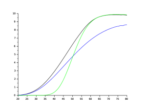
Figure 1: Value function obtained at $t=0$, and $\xi_{2}=50$ as a function of $\xi_{1}\in[20,80]$. Here $N_{\mathrm{in}}=1000$, $N_{\mathrm{rg}}=N_{x}\times N_{w}$, $N_{x}=10$, $N_{w}=1000$ and $N_{\mathrm{m}}=2$. In blue, $\rho$ is constant equal to $-0.8$, in green $\rho$ is constant equal to $0.8$, and in black $\rho\in\{-0.8,0.8\}$.

References

• [1] A. Fahim, N. Touzi, and X. Warin, “A probabilistic numerical method for fully nonlinear parabolic PDEs,” Ann. Appl. Probab., vol. 21, no. 4, pp. 1322–1364, 2011. [Online]. Available: http://dx.doi.org/10.1214/10-AAP723
• [2] P. Cheridito, H. M. Soner, N. Touzi, and N. Victoir, “Second-order backward stochastic differential equations and fully nonlinear parabolic PDEs,” Comm. Pure Appl. Math., vol. 60, no. 7, pp. 1081–1110, 2007. [Online]. Available: http://dx.doi.org/10.1002/cpa.20168
• [3] H. Kaise and W. M. McEneaney, “Idempotent expansions for continuous-time stochastic control: compact control space,” in Proceedings of the 49th IEEE Conference on Decision and Control, Atlanta, Dec. 2010.
• [4] W. M. McEneaney, H. Kaise, and S. H. Han, “Idempotent method for continuous-time stochastic control and complexity attenuation,” in Proceedings of the 18th IFAC World Congress, 2011, Milano, Italie, 2011, pp. 3216–3221.
• [5] I. Kharroubi, N. Langrené, and H. Pham, “A numerical algorithm for fully nonlinear HJB equations: an approach by control randomization,” Monte Carlo Methods Appl., vol. 20, no. 2, pp. 145–165, 2014. [Online]. Available: http://dx.doi.org/10.1515/mcma-2013-0024
• [6] B. Bouchard and N. Touzi, “Discrete-time approximation and Monte-Carlo simulation of backward stochastic differential equations,” Stochastic Process. Appl., vol. 111, no. 2, pp. 175–206, 2004. [Online]. Available: http://dx.doi.org/10.1016/j.spa.2004.01.001
• [7] E. Gobet, J.-P. Lemor, and X. Warin, “A regression-based monte carlo method to solve backward stochastic differential equations,” The Annals of Applied Probability, vol. 15, no. 3, p. 2172–2202, 2005.