Marginalized Particle Filtering and Related Filtering Techniques as Message Passing

Abstract

In this manuscript a factor graph approach is employed to investigate the recursive filtering problem for mixed linear/nonlinear state-space models. Our approach allows us to show that: a) the factor graph characterizing the considered filtering problem is not cycle free; b) in the case of conditionally linear Gaussian systems, applying the sum-product rule, together with different scheduling procedures for message passing, to this graph results in both known and novel filtering techniques. In particular, it is proved that, on the one hand, adopting a specific message scheduling for forward only message passing leads to marginalized particle filtering in a natural fashion; on the other hand, if iterative strategies for message passing are employed, a novel filtering method, dubbed turbo filter for its conceptual resemblance to the turbo decoding methods devised for concatenated channel codes, can be developed.

Keywords: State Space Representation, Hidden Markov Model, Particle Filter, Belief Propagation, Turbo Processing.

1 Introduction

The nonlinear filtering problem consists of inferring the posterior distribution of the hidden state of a nonlinear dynamic system from a set of past and present measurements [1]. It is well known that, if a nonlinear dynamic system can be described by a state-space model (SSM), a general sequential procedure, based on the Bayes’ rule and known as Bayesian filtering, can be easily derived for recursively computing the posterior distribution of the system current state [1]. Unluckily, Bayesian filtering is analytically tractable in few cases for the following two reasons [2]: a) one of the two steps it consists of requires multidimensional integration which, in most cases, does not admit a closed form solution; b) the functional form of the required posterior distribution may not be preserved over successive recursions. For this reason, sequential techniques employed in practice are based on various analytical approximations and, consequently, generate a functional approximation of the desired distribution. Such techniques are commonly divided into local and global methods on the basis of the way posterior distributions are approximated [3, 4, 5]. Local methods, like extended Kalman filtering [6] and unscented filtering [7], are computationally efficient, but may suffer from the problem of error accumulation over time. On the contrary, global methods, like sequential Monte Carlo methods [8, 9] (also known as particle filtering, PF, methods [10, 11, 12]) and point mass filtering [5, 13] may achieve high accuracy at the price, however, of an unmanageable complexity and numerical problems in the presence of a large dimension of system state [14]. These considerations have motivated various research activities focused on the development of novel Bayesian filters able to achieve high accuracy under given computational constraints. Significant results in this research area concern the use of the new representations for complex distributions, like belief condensation filtering [3], and the development of novel filtering techniques combining local and global methods, like marginalized particle filtering (MPF) [15, 16], and other methods originating from it [4, 17, 18]. Note that the last class of methods applies to mixed nonlinear/nonlinear models [19], that is to models whose state can be partitioned in a conditionally linear portion (usually called linear state variable) and in a nonlinear portion (representing the remaining part of system state and called nonlinear state variable). This partitioning of system state allows to combine a global method (e.g., particle filtering) operating on the nonlinear state variable with a local technique (e.g., Kalman filtering) involving the linear state variable only.

In this manuscript the factor graph (FG) approach illustrated by Loeliger et al. in [20] is employed to revisit the problem of recursive Bayesian filtering for mixed linear/nonlinear models from a perspective substantially different from that adopted in MPF [15]. This allows us to shed new light on the problem of filtering for mixed linear/nonlinear models, providing a new interpretation of MPF and paving the way for the development of new filtering techniques. In particular, based on this approach, we are able to show that: a) the considered filtering problem can be formulated as a message massing problem over a specific FG, which, unluckily, is not cycle free; b) in the case of a conditionally linear Gaussian (CLG) SSM [19], MPF results from the application of the sum-product algorithm (SPA) [20, 21], together with a specific scheduling procedure for forward only message passing, to this graph; c) our graphical representation leads, in a natural fashion, to the development of novel filtering methods simplifying and/or generalising it. As far as the last point is concerned, in our work specific attention is paid to the development of a novel iterative filtering technique that exploits the exchange of probabilistic (i.e., soft) messages to progressively refine the posteriors of the linear and nonlinear state variables within each recursion and is dubbed turbo filtering (TF) for its conceptual resemblance to the iterative (i.e., turbo) decoding of concatenated channel codes.

It is important to point that our approach has been inspired by various ideas and results already available in the technical literature concerning different research areas; here, we limit to mention the following relevant facts:

• A mixed linear/nonlinear Markov system can be represented as the concatenation of two interacting subsystems, one governed by linear dynamics, the other one accounting for a nonlinear behavior; conceptually related (finite state) Markov models can be found in data communications and, in particular, in concatenated channel coding (e.g., turbo coding [22]) and in coded transmissions over inter-symbol interference channels for which turbo decoding methods [22, 23] and turbo equalization techniques [24] have been developed, respectively.

• Factor graphs play an essential role in the derivation and interpretation of turbo decoding and equalization [20, 26] (for instance, turbo decoding techniques emerge in a natural fashion from graphical models of codes [27]).

• Both Kalman filtering and particle methods can be viewed as message passing procedures on factor graphs, as shown in [20, 21] and in [28], respectively.

• Various methods to progressively refine distributional approximations through multiple iterations have been developed in the field of Bayesian inference on dynamic systems (even if implementations substantially different from that we devise have been proposed), and, in particular, in expectation propagation in Bayesian networks [29, 30] and in variational Bayesian filtering [4]. Consequently, various links to previous work on Bayesian inference on graphical models and variational Bayes methods [31] can be also established.

The remaining part of this manuscript is organized as follows. The mathematical model of the considered class of mixed linear/nonlinear systems is illustrated in Section 2, whereas a representation of the filtering problem for these systems through a proper FG is provided in Section 3. Then, it is shown that applying the SPA and proper message scheduling strategies to this FG leads to MPF in Section 4. This approach paves the way, in a natural fashion, for the development of simplifications and generalizations of MPF, that are devised in Sections 5 and 6, respectively. The novel filtering methods proposed in this manuscript are compared, in terms of accuracy and computational effort, with MPF in Section 7. Finally, some conclusions are offered in Section 8.

Notations: The probability density function (pdf) of a random vector $\mathbf{R}$ evaluated at point $\mathbf{r}$ is denoted $f(\mathbf{r})$; $\mathcal{N}\left(\mathbf{r};\mathbf{\eta_{r}},\mathbf{C_{r}}\right)$ represents the pdf of a Gaussian random vector $\mathbf{R}$ characterized by the mean $\mathbf{\eta_{r}}$ and covariance matrix $\mathbf{\mathbf{C_{r}}}$ evaluated at point $\mathbf{r}$; the precision (or weight) matrix associated with the covariance matrix $\mathbf{\mathbf{C_{r}}}$ is denoted $\mathbf{\mathbf{W_{r}}}$, whereas the transformed mean vector $\mathbf{\mathbf{W_{r}}\eta_{r}}$ is denoted $\mathbf{\mathbf{w_{r}}}$; $x_{i}$ denotes the $i$-th element of the vector $\mathbf{x}$.

2 System Model

In the following we focus on a discrete-time mixed linear/nonlinear SSM [15], whose hidden state in the $l$-th interval is represented by a $D$-dimensional real vector $\mathbf{x}_{l}\triangleq[x_{0,l},x_{1,l},...,$ $x_{D-1,l}]^{T}$. We assume that this vector can be partitioned as

$$\mathbf{x}_{l}=\left[\left(\mathbf{x}_{l}^{(L)}\right)^{T},\left(\mathbf{x}_{l}^{(N)}\right)^{T}\right]^{T},$$ (1)

where $\mathbf{x}_{l}^{(L)}\triangleq[x_{0,l}^{(L)},x_{1,l}^{(L)},...,x_{D_{L}-1,l}^{(L)}]^{T}$ ($\mathbf{x}_{l}^{(N)}\triangleq[x_{0,l}^{(N)},x_{1,l}^{(N)},...,x_{D_{N}-1,l}^{(L)}]^{T}$) is the so called linear (nonlinear) component of $\mathbf{x}_{l}$ (1), with $D_{L}<D$ ($D_{N}=D-D_{L}$). This partitioning of $\mathbf{x}_{l}$ is accomplished as follows. First, $\mathbf{x}_{l}^{(L)}$ is identified as that portion of $\mathbf{x}_{l}$ (1) characterized by the following two properties:

1. Conditionally linear dynamics - This means that its update equation, conditioned on $\mathbf{x}_{l}^{(N)}$, is linear, so that

   $$\mathbf{x}_{l+1}^{(L)}=\mathbf{A}_{l}^{(L)}\left(\mathbf{x}_{l}^{(N)}\right)\mathbf{x}_{l}^{(L)}+\mathbf{f}_{l}^{(L)}\left(\mathbf{x}_{l}^{(N)}\right)+\mathbf{w}_{l}^{(L)},$$ (2)

   where $\mathbf{f}_{l}^{(L)}\left(\mathbf{x}\right)$ is a time-varying $D_{L}$-dimensional real function, $\mathbf{A}_{l}^{(L)}(\mathbf{x}_{l}^{(N)})$ is a time-varying $D_{L}\times D_{L}$ real matrix and $\mathbf{w}_{l}^{(L)}$ is the $l$-th element of the process noise sequence $\{\mathbf{w}_{k}^{(L)}\}$, which consists of $D_{L}$- dimensional independent and identically distributed (iid) noise vectors.

2. Conditionally linear (or almost linear) dependence of all the available measurements on it - In other words, these quantities, conditioned on $\mathbf{x}_{l}^{(N)}$, exhibit a linear dependence on $\mathbf{x}_{l}^{(L)}$ (additional details about this feature are provided below).

Then, $\mathbf{x}_{l}^{(N)}$ is generated by putting together all the components of $\mathbf{x}_{l}$ that do not belong to $\mathbf{x}_{l}^{(L)}$. For this reason, generally speaking, this vector is characterized by at least one of the following two properties:

a) Nonlinear dynamics - The update equation

$$\mathbf{x}_{l+1}^{(N)}=\mathbf{f}_{l}^{(N)}\left(\mathbf{x}_{l}^{(N)}\right)+\mathbf{A}_{l}^{(N)}\left(\mathbf{x}_{l}^{(N)}\right)\mathbf{x}_{l}^{(L)}+\mathbf{w}_{l}^{(N)}$$ (3)

is assumed in the following for the nonlinear component of system state, where $\mathbf{A}_{l}^{(N)}(\mathbf{x}_{l}^{(N)})$ is a time-varying $D_{N}\times D_{L}$ real matrix, $\mathbf{f}_{l}^{(N)}\left(\mathbf{x}\right)$ is a time-varying $D_{N}$-dimensional real function and $\mathbf{w}_{l}^{(N)}$ is the $l$-th element of the process noise sequence $\{\mathbf{w}_{k}^{(N)}\}$, which consists of $D_{N}$-dimensional iid noise vectors and is statistically independent of $\{\mathbf{w}_{k}^{(L)}\}$.

b) A nonlinear dependence of all the available measurements on it (further details are provided below).

In the following Section we focus on the so-called filtering problem, which concerns the evaluation of the posterior pdf $f(\mathbf{x}_{t}|\mathbf{y}_{1:t})$ at an instant $t>1$, given a) the initial pdf $f(\mathbf{x}_{1})$ and b) the $t\cdot P$-dimensional measurement vector

$$\mathbf{y}_{1:t}=\left[\mathbf{y}_{1}^{T},\mathbf{y}_{2}^{T},...,\mathbf{y}_{t}^{T}\right]^{T},$$ (4)

where $\mathbf{y}_{l}\triangleq[y_{0,l},y_{1,l},$ $...,y_{P-1,l}]^{T}$ denotes the $P$-dimensional real vector collecting all the noisy measurements available at time $l$. As already mentioned above, the measurement vector $\mathbf{y}_{l}$ exhibits a linear (nonlinear) dependence on $\mathbf{x}_{l}^{(L)}$ ($\mathbf{x}_{l}^{(N)}$), so that the model [18]

$$\mathbf{y}_{l}=\mathbf{h}_{l}\left(\mathbf{x}_{l}^{(N)}\right)+\mathbf{B}_{l}\left(\mathbf{x}_{l}^{(N)}\right)\mathbf{x}_{l}^{(L)}+\mathbf{e}_{l}$$ (5)

can be adopted, where $\mathbf{B}_{l}(\mathbf{x}_{l}^{(N)})$ is a time-varying $P\times D_{L}$ real matrix, $\mathbf{h}_{l}(\mathbf{x}_{l}^{(N)})$ is a time-varying $P$-dimensional real function and $\mathbf{e}_{l}$ the $l$-th element of the measurement noise sequence $\left\{\mathbf{e}_{k}\right\}$ consisting of $P$-dimensional iid noise vectors and independent of both $\{\mathbf{w}_{k}^{(N)}\}$ and $\{\mathbf{w}_{k}^{(L)}\}$.

3 Representation of the Filtering Problem via Factor Graphs

Generally speaking, the filtering problem for a SSM described by the Markov model $f(\mathbf{x}_{l+1}|\mathbf{x}_{l})$ and the observation model $f(\mathbf{y}_{l}|\mathbf{x}_{l})$ for any $l$ concerns the computation of the posterior pdf $f(\mathbf{x}_{t}|\mathbf{y}_{1:t})$ for $t\geq 1$ by means of a recursive procedure [1]. It is well known that, if the pdf $f(\mathbf{x}_{1})$ is known, a general Bayesian recursive procedure, consisting of a measurement update step followed by a time update step, can be employed. In practice, in the first step of the $l$-th recursion (with $l=1,2,...,t$) the conditional pdf

$$f\left(\mathbf{x}_{l}\left|\mathbf{y}_{1:l}\right.\right)=f\left(\mathbf{x}_{l}\left|\mathbf{y}_{1:(l-1)}\right.\right)f\left(\mathbf{y}_{l}\left|\mathbf{x}_{l}\right.\right)\frac{1}{f\left(\mathbf{y}_{l}\left|\mathbf{y}_{1:(l-1)}\right.\right)}$$ (6)

is computed on the basis of pdf $f(\mathbf{x}_{l}|\mathbf{y}_{1:(l-1)})$ (evaluated in the last step of the previous recursion), the present measurement vector $\mathbf{y}_{l}$ and the pdf

$$f\left(\mathbf{y}_{l}\left|\mathbf{y}_{1:(l-1)}\right.\right)=\int f\left(\mathbf{y}_{l}\left|\mathbf{x}_{l}\right.\right)f\left(\mathbf{x}_{l}\left|\mathbf{y}_{1:(l-1)}\right.\right)d\mathbf{x}_{l}.$$ (7)

In the second step $f(\mathbf{x}_{l}|\mathbf{y}_{1:l})$ (6) is exploited to compute the pdf

$$f\left(\mathbf{x}_{l+1}\left|\mathbf{y}_{1:l}\right.\right)=\int f\left(\mathbf{x}_{l+1}\left|\mathbf{x}_{l}\right.\right)f\left(\mathbf{x}_{l}\left|\mathbf{y}_{1:l}\right.\right)d\mathbf{x}_{l},$$ (8)

which represents a prediction about the future state $\mathbf{x}_{l+1}$. It is important to point out that: 1) the term $1/f(\mathbf{y}_{l}|\mathbf{y}_{1:(l-1)})$ appearing in the right hand side (RHS) of (6) represents a normalization factor; 2) both (7) and (8) require integration with respect to $\mathbf{x}_{l}$ and this may represent a formidable task when the dimensionality of $\mathbf{x}_{l}$ is large and/or the pdfs appearing in the integrands are not Gaussian; 3) this recursive procedure lends itself to be efficiently represented by a message passing algorithm over a proper FG [28], in which each factor of a product of functions is represented by a distinct node (a rectangle in our diagrams), whereas each variable is associated with a specific (and, usually, unoriented) edge or half edge. As far as the last point is concerned, we also note that the derivation of this FG relies on the fact that the a posteriori pdf $f(\mathbf{x}_{t}|\mathbf{y}_{1:t})$ has the same FG as the joint pdf $f(\mathbf{x}_{t},\mathbf{y}_{1:t})$ (see [20, Sec. II, p. 1297]) and the last pdf can be computed recursively through a procedure similar to that illustrated above, but in which the measurement update (6) and the time update (8) are replaced by

$$f\left(\mathbf{x}_{l},\mathbf{y}_{1:l}\right)=f\left(\mathbf{x}_{l},\mathbf{y}_{1:(l-1)}\right)f\left(\mathbf{y}_{l}\left|\mathbf{x}_{l}\right.\right),$$ (9)

and

$$f\left(\mathbf{x}_{l+1},\mathbf{y}_{1:l}\right)=\int f\left(\mathbf{x}_{l+1}\left|\mathbf{x}_{l}\right.\right)f\left(\mathbf{x}_{l},\mathbf{y}_{1:l}\right)d\mathbf{x}_{l},$$ (10)

respectively, so that the evaluation of the above mentioned normalization factor is no more required. In fact, eqs. (9) and (10) involve only products of pdfs and a sum (i.e., integration) of products, so that they can be represented by means of the FG shown in Fig. 1 (where, following [20], a simplified notation is used for the involved pdfs and the equality constraint node, which represents an equality constraint “function”, that is a Dirac delta function). Since this FG is cycle free, the pdf $f(\mathbf{x}_{l},\mathbf{y}_{1:l})$ can be evaluated applying the well known sum-product rule (i.e., the SPA) to it, i.e. developing a proper mechanism for passing probabilistic messages along this FG (the flow of messages is indicated by red arrows in Fig. 1). In fact, if the input message $\vec{m}_{in}\left(\mathbf{x}_{l}\right)=f(\mathbf{x}_{l},\mathbf{y}_{1:(l-1)})$ enters this FG, the message going out of the equality node is given by

$$\vec{m}_{e}\left(\mathbf{x}_{l}\right)=\vec{m}_{in}\left(\mathbf{x}_{l}\right)f\left(\mathbf{y}_{l}\left|\mathbf{x}_{l}\right.\right),$$ (11)

so that $\vec{m}_{e}\left(\mathbf{x}_{l}\right)=f(\mathbf{x}_{l},\mathbf{y}_{1:l})$ (see (9)); then, the message emerging from the function node referring to the pdf $f(\mathbf{x}_{l+1}|\mathbf{x}_{l})$ is expressed by

$$\vec{m}_{out}\left(\mathbf{x}_{l+1}\right)=\int f\left(\mathbf{x}_{l+1}\left|\mathbf{x}_{l}\right.\right)\vec{m}_{e}\left(\mathbf{x}_{l}\right)d\mathbf{x}_{l},$$ (12)

so that $\vec{m}_{out}\left(\mathbf{x}_{l+1}\right)=f(\mathbf{x}_{l+1},\mathbf{y}_{1:l})=\vec{m}_{in}\left(\mathbf{x}_{l+1}\right)$ (see (10)). From this result it can be easily inferred that the pdf $f(\mathbf{x}_{t},\mathbf{y}_{1:t})$ (and, up to a scale factor, the pdf $f(\mathbf{x}_{t}|\mathbf{y}_{1:t})$) results from the application of the SPA to the overall FG originating from the ordered concatenation of multiple subgraphs, each structured like the one shown in Fig. 1 and associated with $l=1,2,...,t$. In this graph the flow of messages produced by the SPA proceeds from left to right, i.e. the pdf $f(\mathbf{x}_{t},\mathbf{y}_{1:t})$ is generated by a forward only message passing. Note also that, in principle, the desired pdf $f(\mathbf{x}_{t},\mathbf{y}_{1:t})$ is computed as the product between two messages, one for each direction, reaching the rightmost half edge of the overall FG, but one of the two incoming messages for that edge is the constant function $\overleftarrow{m}_{he}(\mathbf{x}_{t})=1$.

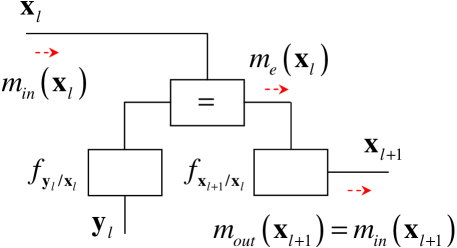
Figure 1: Factor graph representing (9) and (10). The SPA message flow characterizing the $l$-th recursion of Bayesian filtering is indicated by red arrows.

Unluckily, as the size $D$ of $\mathbf{x}_{l}$ (1) gets large, the computational burden associated with (6)-(8) (or, equivalently, (9) and (10)) becomes unmanageable. In principle, a substantial complexity reduction can be achieved decoupling the filtering problem for $\mathbf{x}_{l}^{(L)}$ from that for $\mathbf{x}_{l}^{(N)}$, i.e. the evaluation of $f(\mathbf{x}_{l}^{(L)}|\mathbf{y}_{1:l})$ from that of $f(\mathbf{x}_{l}^{(N)}|\mathbf{y}_{1:l})$. In fact, this approach potentially provides the following two benefits: a) a given filtering problem is turned into a couple of filtering problems of smaller dimensionality and b) some form of computationally efficient standard filtering (e.g., Kalman or extended Kalman filtering) can be hopefully exploited for the linear portion $\mathbf{x}_{l}^{(L)}$ of the state vector $\mathbf{x}_{l}$ (1). As a matter of fact, these principles have been exploited in devising MPF [10, 15] and, as it will become clearer in the following, they must be always kept into account in the derivation of our FG representation. Before illustrating this derivation, however, the measurement and state models on which such a representation relies need to be clearly defined; for this reason, these models are analysed in detail in the following part of this Section. To begin, let us concentrate on the models involved in the filtering problem for $\mathbf{x}_{l}^{(L)}$, i.e. on the evaluation of $f(\mathbf{x}_{l}^{(L)}|\mathbf{y}_{1:l})$, under the assumption that the nonlinear portion $\mathbf{x}_{l}^{(N)}$ of the system state is known for any $l$. In this case, the evaluation of this pdf can benefit not only from the knowledge of $\mathbf{y}_{l}$ (5), but also from that of the quantity (see (3))

$$\mathbf{z}_{l}^{(L)}\triangleq\mathbf{x}_{l+1}^{(N)}-\mathbf{f}_{l}^{(N)}\left(\mathbf{x}_{l}^{(N)}\right)=\mathbf{A}_{l}^{(N)}\left(\mathbf{x}_{l}^{(N)}\right)\mathbf{x}_{l}^{(L)}+\mathbf{w}_{l}^{(N)},$$ (13)

which can be interpreted as a pseudo-measurement [15], since it does not originate from real measurements, but from the constraints expressed by the state equation (3). This leads to considering the overall observation model

$$\begin{array}[c]{c}f\left(\mathbf{y}_{l},\mathbf{z}_{l}^{(L)}\left|\mathbf{x}_{l}^{(L)},\mathbf{x}_{l}^{(N)}\right.\right)\\ =f\left(\mathbf{y}_{l}\left|\mathbf{x}_{l}^{(L)},\mathbf{x}_{l}^{(N)}\right.\right)f\left(\mathbf{z}_{l}^{(L)}\left|\mathbf{x}_{l}^{(L)},\mathbf{x}_{l}^{(N)}\right.\right)\end{array}$$ (14)

for $\mathbf{x}_{l}^{(L)}$, where

$$f\left(\mathbf{y}_{l}\left|\mathbf{x}_{l}^{(L)},\mathbf{x}_{l}^{(N)}\right.\right)=\left.f\left(\mathbf{e}_{l}\right)\right|_{\mathbf{e}_{l}=\mathbf{y}_{l}-\mathbf{B}_{l}\left(\mathbf{x}_{l}^{(N)}\right)\mathbf{x}_{l}^{(L)}-\mathbf{h}_{l}\left(\mathbf{x}_{l}^{(N)}\right)},$$ (15)

and

$$f\left(\mathbf{z}_{l}^{(L)}\left|\mathbf{x}_{l}^{(L)},\mathbf{x}_{l}^{(N)}\right.\right)=\left.f\left(\mathbf{w}_{l}^{(N)}\right)\right|_{\mathbf{w}_{l}^{(N)}=\mathbf{z}_{l}^{(L)}-\mathbf{A}_{l}^{(N)}\left(\mathbf{x}_{l}^{(N)}\right)\mathbf{x}_{l}^{(L)}}.$$ (16)

If the observation model (14) and the state model (see (2))

$$\begin{array}[c]{c}f\left(\mathbf{x}_{l+1}^{(L)}\left|\mathbf{x}_{l}^{(L)},\mathbf{x}_{l}^{(N)}\right.\right)\\ =f_{\mathbf{w}^{(L)}}\left(\mathbf{x}_{l+1}^{(L)}-\mathbf{f}_{l}^{(L)}\left(\mathbf{x}_{l}^{(N)}\right)-\mathbf{A}_{l}^{(L)}\left(\mathbf{x}_{l}^{(N)}\right)\mathbf{x}_{l}^{(L)}\right)\end{array}$$ (17)

are adopted for $\mathbf{x}_{l}^{(L)}$, the graph identified by the blue lines and rectangles appearing in Fig. 1 can be drawn. Then, in principle, if the sum-product rule is applied to it under the assumption that the couple $(\mathbf{x}_{l}^{(N)},\mathbf{x}_{l+1}^{(N)})$ is known for any $l$, the expressions of the messages flowing in the overall graph for the evaluation of $f(\mathbf{x}_{t}^{(L)},\mathbf{y}_{1:t},\mathbf{z}_{1:t}^{(L)})$ can be easily derived. It is important to point out that:

• This graph contains a node which does not refer to the above mentioned density factorizations, but represents the transformation from the couple $(\mathbf{x}_{l}^{(N)},\mathbf{x}_{l+1}^{(N)})$ to $\mathbf{z}_{l}^{(L)}$ (see (13)); this feature of the graph has to be carefully kept into account when deriving message passing algorithms.

• Generally speaking, the evaluation of the conditional pdf $f(\mathbf{z}_{l}^{(L)}|\mathbf{x}_{l}^{(L)},\mathbf{x}_{l}^{(N)})$ requires the knowledge of the joint pdf of $\mathbf{x}_{l+1}^{(N)}$ and $\mathbf{x}_{l}^{(N)}$ conditioned on $\mathbf{x}_{l}^{(L)}$ (see (13)).

The same line of reasoning can be followed for the filtering problem concerning $\mathbf{x}_{l}^{(N)}$. Consequently, in this case the linear portion $\mathbf{x}_{l}^{(L)}$ of the system state is assumed to be known for any $l$ and the pseudo-measurement (see (2))

$$\mathbf{z}_{l}^{(N)}\triangleq\mathbf{x}_{l+1}^{(L)}-\mathbf{A}_{l}^{(L)}\left(\mathbf{x}_{l}^{(N)}\right)\mathbf{x}_{l}^{(L)}=\mathbf{f}_{l}^{(L)}\left(\mathbf{x}_{l}^{(N)}\right)+\mathbf{w}_{l}^{(L)}$$ (18)

is defined. This leads to the overall observation model

$$\begin{array}[t]{c}f\left(\mathbf{y}_{l},\mathbf{z}_{l}^{(N)}\left|\mathbf{x}_{l}^{(N)},\mathbf{x}_{l}^{(L)}\right.\right)=\\ f\left(\mathbf{y}_{l}\left|\mathbf{x}_{l}^{(N)},\mathbf{x}_{l}^{(L)}\right.\right)f\left(\mathbf{z}_{l}^{(N)}\left|\mathbf{x}_{l}^{(N)}\right.\right)\end{array}$$ (19)

for $\mathbf{x}_{l}^{(N)}$, where $f(\mathbf{z}_{l}^{(N)}|\mathbf{x}_{l}^{(N)})$ can be expressed similarly as $f(\mathbf{z}_{l}^{(L)}|\mathbf{x}_{l}^{(L)},\mathbf{x}_{l}^{(N)})$ (see (16)). Then, if the observation model (19) and the state model

$$\begin{array}[c]{c}f\left(\mathbf{x}_{l+1}^{(N)}\left|\mathbf{x}_{l}^{(N)},\mathbf{x}_{l}^{(L)}\right.\right)\\ =f_{\mathbf{w}_{N}}\left(\mathbf{x}_{l+1}^{(N)}-\mathbf{f}_{l}^{(N)}\left(\mathbf{x}_{l}^{(N)}\right)-\mathbf{A}_{l}^{(N)}\left(\mathbf{x}_{l}^{(N)}\right)\mathbf{x}_{l}^{(L)}\right)\end{array}$$ (20)

are adopted for $\mathbf{x}_{l}^{(N)}$, the red graph of Fig. 2 can be drawn and exploited in a similar way as the blue graph for the evaluation of $f(\mathbf{x}_{t}^{(N)},\mathbf{y}_{1:t},\mathbf{z}_{1:t}^{(N)})$, under the assumption that the couple $(\mathbf{x}_{l}^{(L)},$ $\mathbf{x}_{l+1}^{(L)})$ is known for any $l$. Note also that, similarly to what has been mentioned earlier about the conditional pdf $f(\mathbf{z}_{l}^{(L)}|\mathbf{x}_{l}^{(L)},\mathbf{x}_{l}^{(N)})$, the evaluation of $f(\mathbf{z}_{l}^{(N)}|\mathbf{x}_{l}^{(N)})$ requires the knowledge of the joint pdf of $\mathbf{x}_{l+1}^{(L)}$ and $\mathbf{x}_{l}^{(L)}$ conditioned on $\mathbf{x}_{l}^{(N)}$.

Finally, merging the blue graph with the red one (i.e., adding four equality constraint nodes for the variables $\mathbf{x}_{l}^{(L)}$ , $\mathbf{x}_{l}^{(N)}$, $\mathbf{x}_{l+1}^{(L)}$ and $\mathbf{x}_{l+1}^{(N)}$ shared by the red graph and the blue one) produces the overall FG illustrated in Fig. 2. Given this FG, we would like to follow the same line of reasoning as that adopted for the FG of Fig. 1. In other words, given the input messages $\vec{m}_{in}(\mathbf{x}_{l}^{(L)})=f(\mathbf{x}_{l}^{(L)},\mathbf{y}_{1:(l-1)})$ and $\vec{m}_{in}(\mathbf{x}_{l}^{(N)})=f(\mathbf{x}_{l}^{(N)},\mathbf{y}_{1:(l-1)})$ (entering the FG along the half edges associated with $\mathbf{x}_{l}^{(L)}$ and $\mathbf{x}_{l}^{(N)}$, respectively), we would like to derive a forward only message passing algorithm based on this FG and generating the output messages $\vec{m}_{out}(\mathbf{x}_{l+1}^{(L)})=f(\mathbf{x}_{l+1}^{(L)},\mathbf{y}_{1:l})$ and $\vec{m}_{out}(\mathbf{x}_{l+1}^{(N)})=f(\mathbf{x}_{l+1}^{(N)},\mathbf{y}_{1:l})$ (emerging from the FG along the half edges associated with $\mathbf{x}_{l+1}^{(L)}$ and $\mathbf{x}_{l+1}^{(N)}$, respectively) on the basis of the available a priori information and the noisy measurement $\mathbf{y}_{l}$. Unluckily, the new FG, unlike that shown in Fig. 1, is not cycle-free, so that any application of the SPA to it unavoidably leads to approximate results [21], whatever message scheduling procedure [21, 27] is adopted. This consideration must be carefully kept into account in both the derivation of MPF as a message passing algorithm and in the development of possible modifications and generalizations of this technique, as it will become clearer in Sections 4-6.

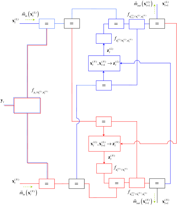
Figure 2: Overall factor graph resulting from the merge of two subgraphs, one referring to filtering for $\mathbf{x}_{l}^{(L)}$ (in blue), the other one to that for $\mathbf{x}_{l}^{(N)}$ (in red).  The equality constraint nodes introduced to connect these subgraphs are identified by black lines. The flow of the messages along the half edges $\mathbf{x}_{l}^{(L)}$ and $\mathbf{x}_{l}^{(N)}$ (input) and that of the messages along the half edges $\mathbf{x}_{l+1}^{(L)}$ and $\mathbf{x}_{l+1}^{(N)}$ (output) are indicated by green arrows.

4 Message Passing in Marginalized Particle Filtering

In the following Section we show how the equations describing the $l$-th recursion of MPF result from the application of the SPA to the FG shown in Fig. 2. However, before illustrating the detailed derivation of such equations, it is important to discuss the following relevant issues. First of all, the MPF technique has been developed for the specific class of GLG SSMs [15, 19], to which we always refer in the following discussion. In particular, in the following we assume that: a) $\{\mathbf{w}_{k}^{(L)}\}$ ($\{\mathbf{w}_{k}^{(N)}\}$) is a Gaussian random process and all its elements have zero mean and covariance $\mathbf{C}_{w}^{(L)}$ ($\mathbf{C}_{w}^{(N)}$) for any $l$; b) $\{\mathbf{e}_{k}^{(L)}\}$ is a Gaussian random process having zero mean and covariance matrix $\mathbf{C}_{e}$ for any $l$; c) all the above mentioned Gaussian processes are statistically independent. Under these assumptions, the pdfs $f(\mathbf{y}_{l}|\mathbf{x}_{l}^{(L)},\mathbf{x}_{l}^{(N})$, $f(\mathbf{z}_{l}^{(L)}|\mathbf{x}_{l}^{(L)})$ and $f(\mathbf{x}_{l+1}^{(L)}|\mathbf{x}_{l}^{(L)},\mathbf{x}_{l}^{(N)})$ (see (15)-(17)) are Gaussian with mean (covariance matrix) $\mathbf{B}_{l}(\mathbf{x}_{l}^{(N)})\mathbf{x}_{l}^{(L)}+\mathbf{h}_{l}(\mathbf{x}_{l}^{(N)})$, $\mathbf{A}_{l}^{(N)}(\mathbf{x}_{l}^{(N)})\,\mathbf{x}_{l}^{(L)}$and $\mathbf{f}_{l}^{(L)}(\mathbf{x}_{l}^{(N)})+\mathbf{A}_{l}^{(L)}(\mathbf{x}_{l}^{(N)})\,\mathbf{x}_{l}^{(L)}$, respectively ($\mathbf{C}_{e}$, $\mathbf{C}_{w}^{(N)}$ and $\mathbf{C}_{w}^{(L)}$, respectively). Similarly, the pdfs $f(\mathbf{z}_{l}^{(N)}|\mathbf{x}_{l}^{(N)})$ and $f(\mathbf{x}_{l+1}^{(N)}|\mathbf{x}_{l}^{(N)},\mathbf{x}_{l}^{(L)})$ (see (19) and (20)) are Gaussian with mean (covariance matrix) $\mathbf{f}_{l}^{(L)}(\mathbf{x}_{l}^{(N)})$ and $\mathbf{f}_{l}^{(N)}(\mathbf{x}_{l}^{(N)})+\mathbf{A}_{l}^{(N)}(\mathbf{x}_{l}^{(N)})\,\mathbf{x}_{l}^{(L)}$, respectively ($\mathbf{C}_{w}^{(L)}$ and $\mathbf{C}_{w}^{(N)}$, respectively).

Secondly, as explained below in detail, the MPF can be interpreted as a forward only message passing algorithm operating over the FG shown in Fig. 2. The scheduling procedure adopted for MPF unavoidably leads to ignoring the evaluation of the pseudo-measurement $\mathbf{z}_{l}^{(N)}$ (18). For this reason, in the following we refer to the simplified FG shown in Fig. 3, which has been obtained from that illustrated in Fig. 2 removing the block representing the transformation from $(\mathbf{x}_{l}^{(L)},\mathbf{x}_{l+1}^{(L)})$ to $\mathbf{z}_{l}^{(N)}$ and the edges referring to the evaluation of the last vector. Note that: a) in the new graph the block referring to the pdf $f(\mathbf{y}_{l}|\mathbf{x}_{l}^{(L)},\mathbf{x}_{l}^{(N})$ appears twice, since this pdf is involved in the two subgraphs shown in Fig. 2; b) some brown edges and equality nodes have been added to feed such blocks with $m_{in}(\mathbf{x}_{l}^{(N)})$ and $m_{in}(\mathbf{x}_{l}^{(L)})$, since these represents the only a priori information available about $\mathbf{x}_{l}^{(N)}$ and $\mathbf{x}_{l}^{(L)}$, respectively, at the beginning of the $l$-th recursion.

Thirdly, in MPF a particle-based model and a Gaussian model are adopted for the input and the output messages referring to $\mathbf{x}_{l}^{(N)}$ and $\mathbf{x}_{l}^{(L)}$, respectively, and the functional structure of the generated messages is preserved in each recursion. More specifically, on the one hand, the a priori information available about $\mathbf{x}_{l}^{(N)}$ at the beginning of the $l$-th recursion is represented by a set of $N_{p}$ particles $S_{l/(l-1)}^{(N)}=\{\mathbf{x}_{l/(l-1),j}^{(N)},\,j=0,1,...,N_{p}-1\}$ and their weights $\{w_{l/(l-1),j},\,j=0,\,1,...,\,N_{p}-1)\}$; following [15], we assume that such weights are uniform (in other words, $w_{l/(l-1),j}=1/N_{p}$ for $j=0,\,1,...,\,N_{p}-1$), so that they can be ignored in the following derivation. On the other hand, the a priori information available about $\mathbf{x}_{l}^{(L)}$ is represented by a set of Gaussian pdfs, each associated with a specific particle; in particular, the Gaussian model $\mathcal{N}(\mathbf{x}_{l}^{(L)};\mathbf{\eta}_{l/(l.-1),j}^{(L)},\mathbf{C}_{l/(l-1),j}^{(L)})$ is associated with the $j$-th particle (with $j=0,\,1,...,\,N_{p}-1$) at the beginning of the same recursion. From the last point it can be inferred that, in developing a message passing algorithm that represents the MPF technique, we can focus on: a) a single particle contained in the input message $m_{in}(\mathbf{x}_{l}^{(N)})$ and, in particular, on the $j$-th particle $\mathbf{x}_{l/(l-1),j}^{(N)}$; b) on the Gaussian model $\mathcal{N}(\mathbf{x}_{l}^{(L)};\mathbf{\eta}_{l/(l.-1),j}^{(L)},\mathbf{C}_{l/(l-1),j}^{(L)})$ associated with that particle. For this reason, we assume that, at the beginning of the $l$-th recursion, our knowledge about $\mathbf{x}_{l}^{(L)}$ and $\mathbf{x}_{l}^{(N)}$ is condensed in the message

$$\vec{m}_{in,j}\left(\mathbf{x}_{l}^{(L)}\right)=\mathcal{N}\left(\mathbf{x}_{l}^{(L)};\mathbf{\eta}_{l/(l.-1),j}^{(L)},\mathbf{C}_{l/(l-1),j}^{(L)}\right)$$ (21)

and in the message

$$\vec{m}_{in,j}\left(\mathbf{x}_{l}^{(N)}\right)=\delta\left(\mathbf{x}_{l}^{(N)}-\mathbf{x}_{l/(l-1),j}^{(N)}\right),$$ (22)

respectively, with $j=0,1,...,N_{p}-1$; these are processed to generate the corresponding output messages $\vec{m}_{out,j}(\mathbf{x}_{l+1}^{(L)})$ and $\vec{m}_{out,j}(\mathbf{x}_{l+1}^{(N)})$, which are required to have the same functional form as $\vec{m}_{in,j}(\mathbf{x}_{l}^{(L)})$ (21) and $\vec{m}_{in,j}(\mathbf{x}_{l}^{(N)})$ (22), respectively. For this reason, the algorithm for computing $\vec{m}_{out,j}(\mathbf{x}_{l+1}^{(N)})$ is expected to generate a new particle $\mathbf{x}_{(l+1)/l,j}^{(N)}$ with a (uniform) weight $w_{(l+1)/l,j}=1/N_{p}$; similarly, that for evaluating $\vec{m}_{out,j}(\mathbf{x}_{l+1}^{(L)})$ is expected to produce a new Gaussian pdf $\mathcal{N}(\mathbf{x}_{l+1}^{(L)};\mathbf{\eta}_{(l+1)/l,j}^{(L)},\mathbf{C}_{(l+1)/l,j}^{(L)})$ associated with the particle $\mathbf{x}_{(l+1)/l,j}^{(N)}$ (note that, in deriving this pdf, possible scale factors are unrelevant and, consequently, can be dropped).

Given $\vec{m}_{in,j}(\mathbf{x}_{l}^{(L)})$ (21) and $\vec{m}_{in,j}(\mathbf{x}_{l}^{(N)})$ (22), if the SPA is applied to the considered graph and the message scheduling illustrated in Fig. 3 (and, as a matter of fact, adopted in MPF) is employed, the steps described below are carried out to evaluate $\vec{m}_{out,j}(\mathbf{x}_{l+1}^{(L)})$ and $\vec{m}_{out,j}(\mathbf{x}_{l+1}^{(N)})$ in the $l$-th recursion of MPF.

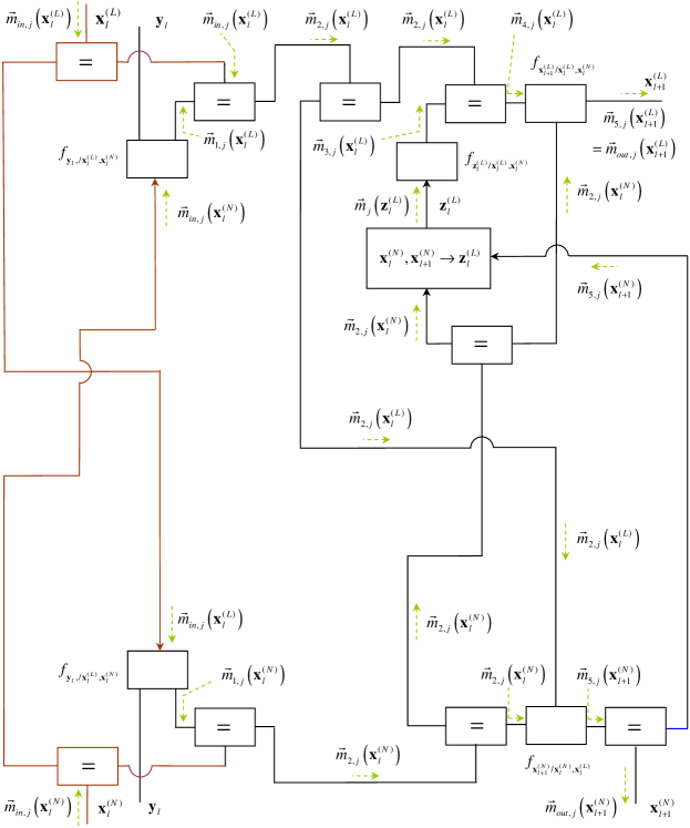
Figure 3: Overall factor graph for the representation of MPF processing; this graph is obtained from the one shown in Fig. 3 removing the part referring to the evaluation of  $\mathbf{z}_{l}^{(N)}$ and inserting two new (brown) equality constraints and some (brown) edges referring to  $\mathbf{x}_{l}^{(L)}$ and $\mathbf{x}_{l}^{(N)}$. The message flow characterizing MPF and referring to the $j$-th particle is also shown.

1. Measurement update for $\mathbf{x}_{l}^{(N)}$ - This step aims at updating the weight of the $j$-th particle $\mathbf{x}_{l/(l-1),j}^{(N)}$ on the basis of the new measurements $\mathbf{y}_{l}$ (this corresponds to step 2) of algorithm 1 in [15, Sec. II]). It involves the computation of the messages

$$\vec{m}_{1,j}\left(\mathbf{x}_{l}^{(N)}\right)=\int f\left(\mathbf{y}_{l}\left|\mathbf{x}_{l}^{(N)},\,\mathbf{x}_{l}^{(L)}\right.\right)\vec{m}_{in,j}\left(\mathbf{x}_{l}^{(L)}\right)d\mathbf{x}_{l}^{(L)}$$ (23)

and

$$\vec{m}_{2,j}\left(\mathbf{x}_{l}^{(N)}\right)=\vec{m}_{in,j}\left(\mathbf{x}_{l}^{(N)}\right)\,\vec{m}_{1,j}\left(\mathbf{x}_{l}^{(N)}\right),$$ (24)

which provides the new importance weight for the considered particle (see Fig. 3). Substituting the expression of $f(\mathbf{y}_{l}\mathbf{x}_{l}^{(N)},\,\mathbf{x}_{l}^{(L)})$ (see (15)) and (21) in (23) produces, after some manipulation (see the Appendix)

$$\vec{m}_{1,j}\left(\mathbf{x}_{l}^{(N)}\right)=\mathcal{N}\left(\mathbf{y}_{l};\mathbf{\eta}_{1,l,j}^{(N)}\left(\mathbf{x}_{l}^{(N)}\right),\mathbf{C}_{1,l,j}^{(N)}\left(\mathbf{x}_{l}^{(N)}\right)\right),$$ (25)

where

$$\mathbf{\eta}_{1,l,j}^{(N)}\left(\mathbf{x}_{l}^{(N)}\right)\triangleq\mathbf{B}_{l}\left(\mathbf{x}_{l}^{(N)}\right)\mathbf{\eta}_{l/(l.-1),j}^{(L)}+\mathbf{h}_{l}\left(\mathbf{x}_{l}^{(N)}\right)$$ (26)

and

$$\mathbf{C}_{1,l,j}^{(N)}\left(\mathbf{x}_{l}^{(N)}\right)\triangleq\mathbf{B}_{l}\left(\mathbf{x}_{l}^{(N)}\right)\mathbf{C}_{l/(l-1),j}^{(L)}\mathbf{B}_{l}\left(\mathbf{x}_{l}^{(N)}\right)^{T}+\mathbf{C}_{e}.$$ (27)

Then, substituting $\vec{m}_{in,j}(\mathbf{x}_{l}^{(N)})$ (22) and $\vec{m}_{1,j}(\mathbf{x}_{l}^{(N)})$ (25) in (24) yields

$$\vec{m}_{2,j}\left(\mathbf{x}_{l}^{(N)}\right)=w_{l,j}\,\delta\left(\mathbf{x}_{l}^{(N)}-\mathbf{x}_{l/(l-1),j}^{(N)}\right),$$ (28)

where

$$w_{l,j}\triangleq\mathcal{N}\left(\mathbf{y}_{l};\mathbf{\eta}_{1,l,j}^{(N)},\mathbf{C}_{1,l,j}^{(N)}\right)$$ (29)

is the new particle weight combining the a priori information about $\mathbf{x}_{l}^{(N)}$ with the information provided by the new measurements; here (see (26) and (27))

$$\mathbf{\eta}_{1,l,j}^{(N)}\triangleq\mathbf{\eta}_{1,l,j}^{(N)}\left(\mathbf{x}_{l/(l-1),j}^{(N)}\right)=\mathbf{B}_{l,j}\mathbf{\eta}_{l/(l.-1),j}^{(L)}+\mathbf{h}_{l,j}$$ (30)

and

$$\mathbf{C}_{1,l,j}^{(N)}\triangleq\mathbf{C}_{1,l,j}^{(N)}\left(\mathbf{x}_{l/(l-1),j}^{(N)}\right)=\mathbf{B}_{l,j}\mathbf{C}_{l/(l-1),j}^{(L)}\mathbf{B}_{l,j}^{T}+\mathbf{C}_{e},$$ (31)

with $\mathbf{h}_{l,j}\triangleq\mathbf{h}_{l}(\mathbf{x}_{l/(l-1),j}^{(N)})$ and $\mathbf{B}_{l,j}\triangleq\mathbf{B}_{l}(\mathbf{x}_{l/(l-1),j}^{(N)})$. In MPF, after normalization of the particle weights $\{w_{l,j}\}$ (i.e., after dividing them by $P_{l}^{(w)}\triangleq{\displaystyle\sum\limits_{j=0}^{N_{p}-1}}w_{l,j}$), particle resampling with replacement is accomplished (this corresponds to step 3) of algorithm 1 in [15, Sec. II]). Note that, even if resampling does not emerge from the application of SPA to the considered graph, its use, as it will become clearer at the end of this Section, plays an important role in the generation of the new particles for $\mathbf{x}_{l+1}^{(N)}$. Moreover, it can be easily incorporated in our message passing; in fact, resampling simply entails that $N_{p}$ particles $\{\mathbf{x}_{l/(l-1),j}^{(N)}\}$ and their associated weights $\{w_{l,j}\}$ (29) are replaced by the new particles $\{\mathbf{x}_{l/l,j}^{(N)}\}$ (forming the new set $S_{l/l}^{(N)}$) and their weights $\{w_{l/l,j}=1/N_{p}\}$, respectively. Consequently, $\vec{m}_{2}(\mathbf{x}_{l}^{(N)})$ (28) is replaced by

$$\vec{m}_{2,j}\left(\mathbf{x}_{l}^{(N)}\right)=\delta\left(\mathbf{x}_{l}^{(N)}-\mathbf{x}_{l/l,j}^{(N)}\right),$$ (32)

since the particle weight does not depend on the index $j$. It is also worth mentioning that, after resampling, the set of Gaussian messages $\{\vec{m}_{in,j}(\mathbf{x}_{l}^{(L)})\}$ (21) needs to be properly reordered and that the messages associated with all the discarded particles are not propagated to the next steps.

2. Measurement update for $\mathbf{x}_{l}^{(L)}$ - This step aims at updating our statistical knowlege about $\mathbf{x}_{l}^{(L)}$ on the basis of the new measurement $\mathbf{y}_{l}$ (and corresponds to step 3-a) of algorithm 1 in [15, Sec. II]). It involves the computation of the messages

$$\vec{m}_{1,j}\left(\mathbf{x}_{l}^{(L)}\right)=\int f\left(\mathbf{y}_{l}\left|\mathbf{x}_{l}^{(L)},\mathbf{x}_{l}^{(N)}\right.\right)\vec{m}_{in,j}\left(\mathbf{x}_{l}^{(N)}\right)d\mathbf{x}_{l}^{(N)}$$ (33)

and

$$\vec{m}_{2,j}\left(\mathbf{x}_{l}^{(L)}\right)=\vec{m}_{in,j}\left(\mathbf{x}_{l}^{(L)}\right)\,\vec{m}_{1,j}\left(\mathbf{x}_{l}^{(L)}\right),$$ (34)

which represents the output of the measurement update for $\mathbf{x}_{l}^{(L)}$ (see Fig. 3). Substituting (15) and (22) in (33) produces (see [32, Par. 2.3.3, eq. (2.115)])

$$\vec{m}_{1,j}\left(\mathbf{x}_{l}^{(L)}\right)=\mathcal{N}\left(\mathbf{y}_{l};\mathbf{B}_{l,j}\mathbf{x}_{l}^{(L)}+\mathbf{h}_{l,j},\mathbf{C}_{e}\right)$$ (35)

which, after some manipulation (in which unrelevant scale factors are dropped), can be put in the Gaussian form

$$\vec{m}_{1,j}\left(\mathbf{x}_{l}^{(L)}\right)=\mathcal{N}\left(\mathbf{x}_{l}^{(L)};\mathbf{\eta}_{1,l,j}^{(L)},\mathbf{C}_{1,l,j}^{(L)}\right),$$ (36)

with

$$\mathbf{w}_{1,l,j}^{(L)}\triangleq\mathbf{W}_{1,l,j}^{(L)}\mathbf{\eta}_{1,l,j}^{(L)}=\mathbf{B}_{l,j}^{T}\mathbf{W}_{e}\left(\mathbf{y}_{l}-\mathbf{h}_{l,j}\right),$$ (37)

$$\mathbf{W}_{1,l,j}^{(L)}\triangleq\left(\mathbf{C}_{1,l,j}^{(L)}\right)^{-1}=\mathbf{B}_{l,j}^{T}\mathbf{W}_{e}\mathbf{B}_{l,j}$$ (38)

and $\mathbf{W}_{e}\triangleq\mathbf{C}_{e}^{-1}$. Then, substituting (21) and (36) in (34) yields

$$\begin{array}[c]{c}\vec{m}_{2,j}\left(\mathbf{x}_{l}^{(L)}\right)=\mathcal{N}\left(\mathbf{x}_{l}^{(L)};\mathbf{\eta}_{l/(l-1),j}^{(L)},\mathbf{C}_{l/(l-1),j}^{(L)}\right)\\ \cdot\mathcal{N}\left(\mathbf{x}_{l}^{(L)};\mathbf{\eta}_{1,l,j}^{(L)},\mathbf{C}_{1,l,j}^{(L)}\right),\end{array}$$ (39)

which can be reformulated as

$$\vec{m}_{2,j}\left(\mathbf{x}_{l}^{(L)}\right)=\mathcal{N}\left(\mathbf{x}_{l}^{(L)};\mathbf{\eta}_{2,l,j}^{(L)},\mathbf{C}_{2,l,j}^{(L)}\right),$$ (40)

if scale factors are ignored; here,

$$\mathbf{w}_{2,l,j}^{(L)}\triangleq\mathbf{W}_{2,l,j}^{(L)}\mathbf{\eta}_{2,l,j}^{(L)}=\mathbf{w}_{l/(l-1),j}^{(L)}+\mathbf{w}_{1,l,j}^{(L)},$$ (41)

$$\mathbf{W}_{2,l,j}^{(L)}\triangleq\left(\mathbf{C}_{2,l,j}^{(L)}\right)^{-1}=\mathbf{W}_{l/(l-1),j}^{(L)}+\mathbf{W}_{1,l,j}^{(L)},$$ (42)

$\mathbf{W}_{l/(l-1),j}^{(L)}\triangleq(\mathbf{C}_{l/(l-1),j}^{(L)})^{-1}$ and $\mathbf{w}_{l/(l-1),j}^{(L)}\triangleq\mathbf{W}_{l/(l-1),j}^{(L)}\mathbf{\eta}_{l/(l-1),j}^{(L)}$.

3. Time update for $\mathbf{x}_{l}^{(N)}$ - This step aims at generating the $j$-th particle for $\mathbf{x}_{l+1}^{(N)}$ and its associated weight (this corresponds to step 3-b) of algorithm 1 in [15, Sec. II]); these information are conveyed by the message $\vec{m}_{5,j}(\mathbf{x}_{l+1}^{(N)})$, which can be expressed as (see Fig. 3)

$$\begin{array}[c]{c}\vec{m}_{5,j}\left(\mathbf{x}_{l+1}^{(N)}\right)=\int\int\,f\left(\mathbf{x}_{l+1}^{(N)}\left|\mathbf{x}_{l}^{(L)},\mathbf{x}_{l}^{(N)}\right.\right)\\ \cdot\vec{m}_{2,j}\left(\mathbf{x}_{l}^{(N)}\right)\,\vec{m}_{2,j}\left(\mathbf{x}_{l}^{(L)}\right)d\mathbf{x}_{l}^{(L)}d\mathbf{x}_{l}^{(N)}.\end{array}$$ (43)

The double integral appearing in the RHS of the last equation can be evaluated as follows. First of all, substituting $\vec{m}_{2,j}(\mathbf{x}_{l}^{(N)})$ (32) in (43) yields

$$\vec{m}_{5,j}\left(\mathbf{x}_{l+1}^{(N)}\right)=\int f\left(\mathbf{x}_{l+1}^{(N)}\left|\mathbf{x}_{l}^{(L)},\mathbf{x}_{l/l,j}^{(N)}\right.\right)\vec{m}_{2,j}\left(\mathbf{x}_{l}^{(L)}\right)d\mathbf{x}_{l}^{(L)}.$$ (44)

Then, substituting the expression of $f(\mathbf{x}_{l+1}^{(N)}|\mathbf{x}_{l}^{(N)},\mathbf{x}_{l}^{(L)})$ (see (20)) and $\vec{m}_{2,j}(\mathbf{x}_{l}^{(L)})$ (40) in (44) yields, after some manipulation, the Gaussian message (see [32, Par. 2.3.3, eq. (2.115)])

$$\vec{m}_{5,j}\left(\mathbf{x}_{l+1}^{(N)}\right)=\mathcal{N}\left(\mathbf{x}_{l+1}^{(N)};\mathbf{\eta}_{5,l,j}^{(N)},\mathbf{C}_{5,l,j}^{(N)}\right),$$ (45)

where

$$\mathbf{\eta}_{5,l,j}^{(N)}\triangleq\mathbf{A}_{l,j}^{(N)}\mathbf{\eta}_{2,l,j}^{(L)}+\mathbf{f}_{l,j}^{(N)},$$ (46)

$$\mathbf{C}_{5,l,j}^{(N)}\triangleq\mathbf{C}_{w}^{(N)}+\mathbf{A}_{l,j}^{(N)}\mathbf{C}_{2,l,j}^{(L)}\left(\mathbf{A}_{l,j}^{(N)}\right)^{T},$$ (47)

$\mathbf{A}_{l,j}^{(N)}\triangleq\mathbf{A}_{l}^{(N)}(\mathbf{x}_{l/l,j}^{(N)})$ and $\mathbf{f}_{l,j}^{(N)}\triangleq\mathbf{f}_{l}^{(N)}(\mathbf{x}_{l/l,j}^{(N)})$. Note that, in principle,

$$\vec{m}_{out,j}\left(\mathbf{x}_{l+1}^{(N)}\right)=\vec{m}_{5,j}\left(\mathbf{x}_{l+1}^{(N)}\right),$$ (48)

as it can be easily inferred from Fig. 3. However, as already mentioned above, in MPF the output message $\vec{m}_{out}^{(j)}(\mathbf{x}_{l+1}^{(N)})$ is required to have the same functional form as $\vec{m}_{in}^{(j)}(\mathbf{x}_{l}^{(N)})$ (22). This result can be achieved a) sampling the Gaussian function $\mathcal{N}(\mathbf{x}_{l+1}^{(N)};\mathbf{\eta}_{5,l,j}^{(N)},\mathbf{C}_{5,l,j}^{(N)})$ (see (45)), that is drawing a sample $\mathbf{x}_{(l+1)/l,j}^{(N)}$ from it and b) assigning to the sample $\mathbf{x}_{(l+1)/l,j}^{(N)}$ a probability $w_{(l+1)/l,j}$ equal to the weight $w_{l/l,j}=1/N_{p}$ (originating from resampling). It is worth pointing out that: 1) the particles $\{\mathbf{x}_{(l+1)/l,j}^{(N)}\}$ form the new set $S_{(l+1)/l}$; 2) in accomplishing step a) of this procedure, it may be useful to introduce artificial noise (this can be simply done adding the same positive quantity to the diagonal elements of the matrix $\mathbf{C}_{w}^{(N)}$ appearing in the RHS of (47)) in order to mitigate the so called degeneracy problem [1, 34]. If this approach is adopted, the message $\vec{m}_{5,j}(\mathbf{x}_{l+1}^{(N)})$ (45) is replaced by

$$\vec{m}_{5,j}\left(\mathbf{x}_{l+1}^{(N)}\right)=\delta\left(\mathbf{x}_{l+1}^{(N)}-\mathbf{x}_{(l+1)/l,j}^{(N)}\right),$$ (49)

which emerges from the graph as $\vec{m}_{out,j}(\mathbf{x}_{l+1}^{(N)})$. This message is also used in the time update for $\mathbf{x}_{l}^{(L)}$, as illustrated in the next step.

4. Time update for $\mathbf{x}_{l}^{(L)}$ - This step aims at generating a new Gaussian pdf associated with the $j$-th particle $\mathbf{x}_{(l+1)/l,j}^{(N)}$ and conveyed by $\vec{m}_{5,j}(\mathbf{x}_{l+1}^{(L)})=\vec{m}_{out,j}(\mathbf{x}_{l+1}^{(L)})$ (this corresponds to step 3-c) of algorithm 1 in [15, Sec. II]). However, before doing that, a further measurement update is accomplished on the basis of the pseudo-measurement $\mathbf{z}_{l}^{(L)}$ (13). This involves the evaluation of the messages $\vec{m}_{j}(\mathbf{z}_{l}^{(L)})$,

$$\vec{m}_{3,j}\left(\mathbf{x}_{l}^{(L)}\right)=\int\vec{m}_{j}\left(\mathbf{z}_{l}^{(L)}\right)\,f\left(\mathbf{z}_{l}^{(L)}\left|\mathbf{x}_{l}^{(L)},\mathbf{x}_{l}^{(N)}\right.\right)d\mathbf{z}_{l}^{(L)}$$ (50)

and

$$\vec{m}_{4,j}\left(\mathbf{x}_{l}^{(L)}\right)=\vec{m}_{2,j}\left(\mathbf{x}_{l}^{(L)}\right)\,\vec{m}_{3,j}\left(\mathbf{x}_{l}^{(L)}\right),$$ (51)

as shown in Fig. 3. Generally speaking, the message $\vec{m}_{j}(\mathbf{z}_{l}^{(L)})$ can be expressed as

$$\begin{array}[c]{c}\vec{m}_{j}\left(\mathbf{z}_{l}^{(L)}\right)=\int\int f\left(\mathbf{z}_{l}^{(L)}\left|\mathbf{x}_{l}^{(N)},\mathbf{x}_{l+1}^{(N)}\right.\right)\\ \cdot f\left(\mathbf{x}_{l+1}^{(N)}\left|\mathbf{x}_{l}^{(N)}\right.\right)\,f\left(\mathbf{x}_{l}^{(N)}\right)d\mathbf{x}_{l}^{(N)}d\mathbf{x}_{l+1}^{(N)}.\end{array}$$ (52)

However, since in this case $f(\mathbf{x}_{l}^{(N)})=\delta(\mathbf{x}_{l}^{(N)}-\mathbf{x}_{l/l,j}^{(N)})$, $f(\mathbf{x}_{l+1}^{(N)}|\mathbf{x}_{l}^{(L)})=\delta(\mathbf{x}_{l}^{(N+1)}-\mathbf{x}_{(l+1)/l,j}^{(N)})$ can be assumed (see $\vec{m}_{2,j}(\mathbf{x}_{l}^{(N)})$ (32) and $\vec{m}_{5,j}(\mathbf{x}_{l+1}^{(N)})$ (49), respectively), eq. (52) easily leads to the expression

$$\vec{m}_{j}\left(\mathbf{z}_{l}^{(L)}\right)=f\left(\mathbf{z}_{l}^{(L)}\left|\mathbf{x}_{l/l,j}^{(N)},\mathbf{x}_{(l+1)/l,j}^{(N)}\right.\right)=\delta\left(\mathbf{z}_{l}^{(L)}-\mathbf{z}_{l,j}^{(L)}\right),$$ (53)

where

$$\mathbf{z}_{l,j}^{(L)}\triangleq\mathbf{x}_{(l+1)/l,j}^{(N)}-\mathbf{f}_{l,j}^{(N)}.$$ (54)

Then, substituting (53) and the expression of $f(\mathbf{z}_{l}^{(L)}|\mathbf{x}_{l}^{(L)},\mathbf{x}_{l}^{(N)})$ (see (16)) in (50) yields

$$\vec{m}_{3,j}\left(\mathbf{x}_{l}^{(L)}\right)=\mathcal{\mathcal{N}}\left(\mathbf{z}_{l,j}^{(L)};\mathbf{A}_{l,j}^{(N)}\mathbf{x}_{l}^{(L)},\mathbf{C}_{w}^{(N)}\right).$$ (55)

Finally, substituting the last expression and (40) in (51) produces

$$\begin{array}[c]{c}\vec{m}_{4,j}\left(\mathbf{x}_{l}^{(L)}\right)=\mathcal{N}\left(\mathbf{x}_{l}^{(L)};\mathbf{\eta}_{2,l,j}^{(L)},\mathbf{C}_{2,l,j}^{(L)}\right)\\ \cdot\mathcal{\mathcal{N}}\left(\mathbf{z}_{l,j}^{(L)};\mathbf{A}_{l,j}^{(N)}\mathbf{x}_{l}^{(L)},\mathbf{C}_{w}^{(N)}\right),\end{array}$$ (56)

which, after some manipulation (in which unrelevant scale factors are dropped), can be rewritten as

$$\vec{m}_{4,j}\left(\mathbf{x}_{l}^{(L)}\right)=\mathcal{N}\left(\mathbf{x}_{l}^{(L)};\mathbf{\eta}_{4,l,j}^{(L)},\mathbf{C}_{4,l,j}^{(L)}\right),$$ (57)

where

$$\mathbf{w}_{4,l,j}^{(L)}\triangleq\mathbf{W}_{4,l,j}^{(L)}\mathbf{\eta}_{4,l,j}^{(L)}=\mathbf{w}_{2,l,j}^{(L)}+\left(\mathbf{A}_{l,j}^{(N)}\right)^{T}\mathbf{W}_{w}^{(N)}\mathbf{z}_{l,j}^{(L)},$$ (58)

$$\mathbf{W}_{4,l,j}^{(L)}\triangleq\left(\mathbf{C}_{4,l,j}^{(L)}\right)^{-1}=\mathbf{W}_{2,l,j}^{(L)}+\left(\mathbf{A}_{l,j}^{(N)}\right)^{T}\mathbf{W}_{w}^{(N)}\mathbf{A}_{l,j}^{(N)}$$ (59)

and $\mathbf{W}_{w}^{(N)}\triangleq[\mathbf{C}_{w}^{(N)}]^{-1}$.

The last part of the time update step for $\mathbf{x}_{l}^{(L)}$ requires the evaluation of the output message

$$\begin{array}[c]{c}\vec{m}_{5,j}\left(\mathbf{x}_{l+1}^{(L)}\right)=\int\int\,f\left(\mathbf{x}_{l+1}^{(L)}\left|\mathbf{x}_{l}^{(L)},\mathbf{x}_{l}^{(N)}\right.\right)\\ \cdot\vec{m}_{4,j}\left(\mathbf{x}_{l}^{(L)}\right)\,\vec{m}_{2,j}\left(\mathbf{x}_{l}^{(N)}\right)\,d\mathbf{x}_{l}^{(L)}d\mathbf{x}_{l}^{(N)},\end{array}$$ (60)

which, similarly as $\vec{m}_{5,j}(\mathbf{x}_{l+1}^{(N)})$ (43), requires double integration. Substituting $\vec{m}_{2,j}(\mathbf{x}_{l}^{(N)})$ (32) in the RHS of the last expression yields

$$\vec{m}_{5,j}\left(\mathbf{x}_{l+1}^{(L)}\right)=\int\,f\left(\mathbf{x}_{l+1}^{(L)}\left|\mathbf{x}_{l}^{(L)},\mathbf{x}_{l/l,j}^{(N)}\right.\right)\,\vec{m}_{4,j}\left(\mathbf{x}_{l}^{(L)}\right)\,d\mathbf{x}_{l}^{(L)}.$$ (61)

Then, substituting the expression of $f(\mathbf{x}_{l+1}^{(L)}|\mathbf{x}_{l}^{(L)},\mathbf{x}_{l/(l-1),j}^{(N)})$ (see (17)) and (57) in the last equation gives (see [32, Par. 2.3.3, eq. (2.115)])

$$\begin{array}[c]{c}\vec{m}_{5,j}\left(\mathbf{x}_{l+1}^{(L)}\right)=\mathcal{N}\left(\mathbf{x}_{l+1}^{(L)};\mathbf{\eta}_{5,l,j}^{(L)},\mathbf{C}_{5,l,j}^{(L)}\right)\\ =\vec{m}_{out,j}\left(\mathbf{x}_{l+1}^{(L)}\right)\text{,}\end{array}$$ (62)

where

$$\mathbf{\eta}_{5,l,j}^{(L)}\triangleq\mathbf{A}_{l,j}^{(L)}\mathbf{\eta}_{4,l,j}^{(L)}+\mathbf{f}_{l,j}^{(L)}=\mathbf{\eta}_{(l+1)/l,j}^{(L)},$$ (63)

$$\mathbf{C}_{5,l,j}^{(L)}\triangleq\mathbf{C}_{w}^{(L)}+\mathbf{A}_{l,j}^{(L)}\mathbf{C}_{4,l,j}^{(L)}\left(\mathbf{A}_{l,j}^{(L)}\right)^{T}=\mathbf{C}_{(l+1)/l,j}^{(L)},$$ (64)

$\mathbf{f}_{l,j}^{(L)}\triangleq\mathbf{f}_{l}^{(L)}(\mathbf{x}_{l/l,j}^{(N)})$ and $\mathbf{A}_{l,j}^{(L)}\triangleq\mathbf{A}_{l}^{(L)}(\mathbf{x}_{l/l,j}^{(N)})$. The evaluation of $\vec{m}_{out,j}(\mathbf{x}_{l+1}^{(L)})$ (62) concludes the MPF message passing procedure, which needs to be carried out for each of the $N_{p}$ particles available at the beginning of the $l$-th recursion. Note that this procedure needs a proper inizialization (this corresponds to step 1) of algorithm 1 in [15, Sec. II]). In practice, before starting the first recursion (corresponding to $l=1$), the set $S_{1/0}^{(N)}=\{\mathbf{x}_{1/0,j}^{(N)},\,j=0,1,...,N_{p}-1\}$, consisting of $N_{p}$ particles, is generated for $\mathbf{x}_{1}^{(N)}$ sampling the pdf

$$f\left(\mathbf{x}_{1}^{(N)}\right)=\int f\left(\mathbf{x}_{1}\right)d\mathbf{x}_{1}^{(L)},$$ (65)

and the same weight $w_{1/0}=1/N_{p}$ and Gaussian model $\mathcal{N}(\mathbf{x}_{1}^{(L)};\mathbf{\eta}_{1/0}^{(L)},\mathbf{C}_{1/0}^{(L)})$ for $\mathbf{x}_{1}^{(L)}$ are assigned to each of them.

Finally, it is worth pointing out that: 1) the processing accomplished in the measurement and time update for $\mathbf{x}_{l}^{(L)}$ can be interpreted as a form of Kalman filtering, in which both the real measurement $\mathbf{y}_{l}$ and the pseudo-measurement $\mathbf{z}_{l}^{(L)}$ are processed [15]; 2) in the $l$-th recursion estimates of $\mathbf{x}_{l}^{(N)}$ and $\mathbf{x}_{l}^{(L)}$ can be evaluated as $\mathbf{\hat{x}}_{l}^{(N)}=\sum_{j=0}^{N_{p}-1}w_{l,j}\mathbf{x}_{l/(l-1),j}^{(N)}/P_{l}^{(w)}$ (see (28)) and as $\mathbf{\hat{x}}_{l}^{(L)}=\sum_{j=0}^{N_{p}-1}\mathbf{\eta}_{4,l,j}^{(L)}/N_{{}_{p}}$ (see (58)), respectively; 3) the result expressed by eq. (45) shows that, generally speaking, the statistical representation generated by the SPA for the state $\mathbf{x}_{l+1}^{(N)}$ is a Gaussian mixture (GM), whose $N_{p}$ components have the same weight (equal to $1/N_{p}$) because resampling is always used in step 1. The last point leads to the conclusion that, if resampling was not accomplished in the $l$-th recursion, the weight of the $j$-th component of this GM would be proportional by $w_{l,j}$ (29); this would unavoidably raise the problem of sampling a GM with unequally weighted components in generating the particle set $S_{l/(l+1)}^{(N)}$ and that of properly handling the resulting pseudo-measurements $\{\mathbf{z}_{l,j}^{(L)}\}$. These considerations motivate the use of resampling in each recursion, indipendently of the effective sample size [1] characterizing the particle set $S_{l/(l-1)}^{(N)}$.

5 Simplifying Marginalized Particle Filtering

The MPF derivation illustrated in the last two Sections unveils the real nature of MPF and its limitations, and shows the inner structure of the processing accomplished within each step. For these reasons, it paves the way for the development of new filtering methods related to MPF. In this Section we exploit our FG-based representation of Bayesian filtering to develop reduced complexity alternatives to MPF by simplifying the message passing derived in the previous Section. It is worth mentioning that some methods for reducing MPF computational complexity [16] have been already proposed in the technical literature  [4], [17], [18]. In particular, the method proposed in [4] and [17] is based on representing the particle set for $\mathbf{x}_{l}^{(N)}$ as a single particle (that corresponds to the center of mass of the set itself), so that a single Kalman filter is employed in updating the statistics of the linear component $\mathbf{x}_{l}^{(L)}$; consequently, the statistical knowledge about $\mathbf{x}_{l}^{(L)}$ is condensed in the single message

$$\vec{m}_{in}\left(\mathbf{x}_{l}^{(L)}\right)=\mathcal{N}\left(\mathbf{x}_{l}^{(L)};\mathbf{\eta}_{l/(l.-1)}^{(L)},\mathbf{C}_{l/(l-1)}^{(L)}\right),$$ (66)

instead of the $N_{p}$ messages $\{\vec{m}_{in,j}(\mathbf{x}_{l}^{(L)})\}$ (21). Unluckily, this simplified MPF algorithm works well only if the posterior distribution of $\mathbf{x}_{l}^{(N)}$ is unimodal. Its generalization to the case in which the posterior distribution of $\mathbf{x}_{l}^{(N)}$ is multimodal has been illustrated later in [18]. In the proposed technique the particles are partitioned into $K_{l}$ groups or clusters (the parameter $K_{l}$ is required to equal the number of modes of the posterior density of $\mathbf{x}_{l}^{(N)}$) and each group is represented by a single particle that corresponds to its center of mass; this allows to reduce the overall number of Kalman filters from $N_{p}$ to $K_{l}$. The implementation of this technique requires, however, solving the following two specific problems: a) identifying the number of modes of the posterior distribution of $\mathbf{x}_{l}^{(N)}$; b) partitioning the particles into clusters according to a grouping method in each recursion. Unluckily, practical solutions for suche problems have not been proposed in [18].

Our derivation of simplified algorithms has been only partly inspired by the manuscripts cited above. In fact, first of all, it relies on the following specific methods: a) a set of $N_{p}$ equal weight particles $\{\mathbf{x}_{j};\,j=0,\,1,...,\,N_{p}-1\}$ is represented through its center of mass

$$\mathbf{\bar{x}}\triangleq\frac{1}{N_{p}}\sum_{j=0}^{N_{p}-1}\mathbf{x}_{j}\text{,}$$ (67)

as already suggested in [17] and [18], when the computation of a message referring to $\mathbf{x}_{l}^{(L)}$ involves the particle-based representation of $\mathbf{x}_{l}^{(N)}$; b) a set of $N_{p}$ Gaussian messages $\{\mathcal{N}(\mathbf{x};\mathbf{\eta}_{j},\mathbf{C}_{j});\,j=0,\,1,...,\,N_{p}-1\}$, that refer to a set of $N_{p}$ equal weight particles, is represented as the $N_{p}-$component GM

$$f_{GM}\left(\mathbf{x}\right)\triangleq\frac{1}{N_{p}}\sum_{j=0}^{N_{p}-1}\mathcal{N}\left(\mathbf{x};\mathbf{\eta}_{j},\mathbf{C}_{j}\right),$$ (68)

and this GM is approximated through its projection onto the Gaussian pdf $f_{G}\left(\mathbf{x}\right)=\mathcal{N}\left(\mathbf{x};\mathbf{\eta}_{G},\mathbf{C}_{G}\right)$, where $\mathbf{\eta}_{G}$ and $\mathbf{C}_{G}$ are selected as

$$\mathbf{\eta}_{G}\triangleq\frac{1}{N_{p}}\sum_{j=0}^{N_{p}-1}\mathbf{\eta}_{j}$$ (69)

and

$$\begin{array}[t]{c}\mathbf{C}_{G}=(1/N_{p})\sum_{j=0}^{N_{p}-1}\mathbf{C}_{j}\\ -\mathbf{\eta}_{G}\left(\mathbf{\eta}_{G}\right)^{T}+(1/N_{p})\sum_{j=0}^{N_{p}-1}\mathbf{\eta}_{j}\left(\mathbf{\eta}_{j}\right)^{T}\end{array}$$ (70)

respectively, so that the mean and covariance of $f_{GM}\left(\mathbf{x}\right)$ (68) are preserved (e.g., see [33, Sec. IV]). Secondly, as far as the messages $\{\vec{m}_{in,j}(\mathbf{x}_{l}^{(L)})\}$ (21) are concerned, we do not adopt the approximations proposed in [4], [17] and [18]. In fact, we focus on the following two cases: case #1 - the messages $\{\vec{m}_{in,j}(\mathbf{x}_{l}^{(L)})\}$ are all different but, when needed in message passing, are condensed in the single message (66), where $\mathbf{\eta}_{l/(l.-1)}^{(L)}$ and $\mathbf{C}_{l/(l-1)}^{(L)}$ are given by (69) and (70), respectively, with $\mathbf{\eta}_{j}=\mathbf{\eta}_{l/(l.-1),j}^{(L)}$ and $\mathbf{C}_{j}=\mathbf{C}_{l/(l-1),j}^{(L)}$; b) case #2 - the messages $\{\vec{m}_{in,j}(\mathbf{x}_{l}^{(L)})\}$ have different means, but their covariance matrices $\{\mathbf{C}_{l/(l-1),j}^{(L)}\}$ are all equal (their common value is denoted $\mathbf{\tilde{C}}_{l/(l-1)}^{(L)}$ in the following). In both cases our simplifications aim at minimizing the overall number of a) Cholesky decompositions for the generation of the new particle set $S_{(l+1)/l}$ (such decompositions are required for the $N_{p}$ matrices $\{\mathbf{C}_{5,l,j}^{(L)}\}$ (47)) and b) matrix inversions; such inversions are needed to compute: a) the $N_{p}$ matrices $\{\mathbf{W}_{1,l,j}^{(N)}\triangleq(\mathbf{C}_{1,l,j}^{(N)})^{-1}\}$ (required in the evaluation of the weights $\{w_{l,j}\}$ on the basis of (29)); b) the $N_{p}$ matrices $\{\mathbf{W}_{l/(l-1),j}^{(L)}\}$ (required to evaluate the vectors $\{\mathbf{w}_{2,l,j}^{(L)}\}$ (41) and the matrices $\{\mathbf{W}_{2,l,j}^{(L)}\}$ (42)); c) the $N_{p}$ matrices $\{\mathbf{C}_{2,l,j}^{(L)}\}$ (employed in (47)); c) the $N_{p}$ matrices $\{\mathbf{C}_{4,l,j}^{(L)}\}$ (employed in (64)).

Based on the methods illustrated above, our simplified versions of MPF are derived as follows. First of all, in the measurement update for $\mathbf{x}_{l}^{(N)}$, we use a single covariance matrix in the Gaussian pdf appearing in the RHS of (29); in other words, the $j$-th weigth $w_{l,j}$ is computed as

$$w_{l,j}\triangleq\mathcal{N}\left(\mathbf{y}_{l};\mathbf{\eta}_{1,l,j}^{(N)},\mathbf{C}_{1,l}^{(N)}\right),$$ (71)

where $\mathbf{C}_{1,l}^{(N)}$ is evaluated on the basis of (70) (see also (69)), setting $\mathbf{\eta}_{j}=\mathbf{\eta}_{1,l,j}^{(N)}$ (30) and $\mathbf{C}_{j}=\mathbf{C}_{1,l,j}^{(N)}$ (31) for any $j$.

Second, in the measurement update for $\mathbf{x}_{l}^{(L)}$, the particle set $S_{l/(l-1)}^{(N)}$ is condensed in its center of mass $\mathbf{\bar{x}}_{l/(l-1)}^{(N)}$ (see (67)). Consequently, the message $\vec{m}_{1,j}(\mathbf{x}_{l}^{(L)})$ (35) is replaced by its particle-independent form

$$\vec{m}_{1}\left(\mathbf{x}_{l}^{(L)}\right)=\mathcal{N}\left(\mathbf{y}_{l};\mathbf{\bar{B}}_{l}\mathbf{x}_{l}^{(L)}+\mathbf{\bar{h}}_{l},\mathbf{C}_{e}\right)$$ (72)

where $\mathbf{\bar{B}}_{l}\triangleq\mathbf{B}_{l}(\mathbf{\bar{x}}_{l/(l-1)}^{(N)})$ and $\mathbf{\bar{h}}_{l}\triangleq\mathbf{h}_{l}(\mathbf{\bar{x}}_{l/(l-1)}^{(N)})$. This message, similarly as (35), can be put in the Gaussian form (see (36)-(38))

$$\vec{m}_{1}\left(\mathbf{x}_{l}^{(L)}\right)=\mathcal{N}\left(\mathbf{x}_{l}^{(L)};\mathbf{\eta}_{1,l}^{(L)},\mathbf{C}_{1,l}^{(L)}\right),$$ (73)

where

$$\mathbf{w}_{1,l}^{(L)}\triangleq\mathbf{W}_{1,l}^{(L)}\mathbf{\eta}_{1,l}^{(L)}=\mathbf{\bar{B}}_{l}^{T}\mathbf{W}_{e}\left(\mathbf{y}_{l}-\mathbf{\bar{h}}_{l}\right)$$ (74)

and

$$\mathbf{W}_{1,l}^{(L)}\triangleq\left(\mathbf{C}_{1,l}^{(L)}\right)^{-1}=\mathbf{\bar{B}}_{l}^{T}\mathbf{W}_{e}\mathbf{\bar{B}}.$$ (75)

This allows us to replace the message $\vec{m}_{2,j}(\mathbf{x}_{l}^{(L)})$ (40) with its particle-independent counterpart

$$\vec{m}_{2}\left(\mathbf{x}_{l}^{(L)}\right)=\mathcal{N}\left(\mathbf{x}_{l}^{(L)};\mathbf{\eta}_{2,l}^{(L)},\mathbf{C}_{2,l}^{(L)}\right),$$ (76)

where $\mathbf{w}_{2,l}^{(L)}\triangleq\mathbf{W}_{2,l}^{(L)}\mathbf{\eta}_{2,l}^{(L)}$ and $\mathbf{W}_{2,l}^{(L)}\triangleq(\mathbf{C}_{2,l}^{(L)})^{-1}$ are easily obtained from (41) and (42) replacing a) $\mathbf{w}_{1,l,j}^{(L)}$  and $\mathbf{W}_{1,l,j}^{(L)}$ with $\mathbf{w}_{1,l}^{(L)}$ (74) and $\mathbf{W}_{1,l}^{(L)}$ (75), respectively; b) $\mathbf{w}_{l/(l-1),j}^{(L)}$ and $\mathbf{W}_{l/(l-1),j}^{(L)}$ with $\mathbf{w}_{l/(l-1)}^{(L)}\triangleq\mathbf{W}_{l/(l-1)}^{(L)}\mathbf{\eta}_{l/(l-1)}^{(L)}$ and $\mathbf{W}_{l/(l-1)}^{(L)}\triangleq(\mathbf{C}_{l/(l-1)}^{(L)})^{-1}$ ($\mathbf{\eta}_{l/(l.-1)}^{(L)}$ and $\mathbf{C}_{l/(l-1)}^{(L)}$ are given by (69) and (70), respectively, with $\mathbf{\eta}_{j}=\mathbf{\eta}_{l/(l.-1),j}^{(L)}$ and $\mathbf{C}_{j}=\mathbf{C}_{l/(l-1),j}^{(L)}$). Note that, since the precision matrix $\mathbf{W}_{2,l}^{(L)}$ is particle-independent, a single matrix $\mathbf{C}_{2,l}^{(L)}$ has to be computed for the next step.

Thirdly, in the time update for $\mathbf{x}_{l}^{(N)}$, the message $\vec{m}_{2}(\mathbf{x}_{l}^{(L)})$ (76) can be used in place of $\vec{m}_{2,j}(\mathbf{x}_{l}^{(L)})$ (40) in the evaluation of $\vec{m}_{5,j}(\mathbf{x}_{l+1}^{(N)})$ (see (44) and Fig. 3). This leads to the particle-dependent message

$$\vec{m}_{5,j}\left(\mathbf{x}_{l+1}^{(N)}\right)=\mathcal{N}\left(\mathbf{x}_{l+1}^{(N)};\mathbf{\eta}_{5,l,j}^{(N)},\mathbf{C}_{5,l,j}^{(N)}\right),$$ (77)

where $\mathbf{\eta}_{5,l,j}^{(N)}$ and $\mathbf{C}_{5,l,j}^{(N)}$ are obtained from (46) and (47), respectively, replacing $\mathbf{\eta}_{2,l,j}^{(L)}$ and $\mathbf{C}_{2,l,j}^{(L)}$ with $\mathbf{\eta}_{2,l}^{(L)}$ and $\mathbf{C}_{2,l}^{(L)}$, respectively. Then, to simplify the generation of the new particle set $S_{(l+1)/l}^{(N)}$, the covariance matrices $\{\mathbf{C}_{5,l,j}^{(N)}\}$ are condensed in a single matrix $\mathbf{C}_{5,l}^{(N)}$ using (70) (see also (69)) with $\mathbf{\eta}_{j}=\mathbf{\eta}_{5,l,j}^{(N)}=\mathbf{A}_{l,j}^{(N)}\mathbf{\eta}_{2,l}^{(L)}+\mathbf{f}_{l,j}^{(N)}$ and $\mathbf{C}_{j}=\mathbf{C}_{5,l,j}^{(N)}=\mathbf{C}_{w}^{(N)}+\mathbf{A}_{l,j}^{(N)}\mathbf{C}_{2,l}^{(L)}(\mathbf{A}_{l,j}^{(N)})^{T}$; consequently, the particle generation mechanism for $\mathbf{x}_{l+1}^{(N)}$ requires computing the Cholesky decomposition of a single matrix (namely, $\mathbf{C}_{5,l}^{(N)}$), since it is based on the modified message

$$\vec{m}_{5}\left(\mathbf{x}_{l+1}^{(N)}\right)=\mathcal{N}\left(\mathbf{x}_{l+1}^{(N)};\mathbf{\eta}_{5,l,j}^{(N)},\mathbf{C}_{5,l}^{(N)}\right),$$ (78)

which depends on the particle index $j$ through the mean vector $\mathbf{\eta}_{5,l,j}^{(N)}$ only.

Finally, in the time update for $\mathbf{x}_{l}^{(L)}$, the pdf

$$f\left(\mathbf{z}_{l}^{(L)}\left|\mathbf{x}_{l}^{(L)}\right.\right)=\mathcal{\mathcal{N}}\left(\mathbf{z}_{l}^{(L)};\mathbf{\bar{A}}_{l}^{(N)}\mathbf{x}_{l}^{(L)},\mathbf{C}_{w}^{(N)}\right)$$ (79)

is employed in the evaluation of $\vec{m}_{3,j}(\mathbf{x}_{l}^{(L)})$ through (50), where $\mathbf{\bar{A}}_{l}^{(N)}=\mathbf{A}_{l}^{(N)}(\mathbf{\bar{x}}_{l/l}^{(N)})$ and $\mathbf{\bar{x}}_{l/l}^{(N)}$ denotes the center of mass of the particle set $S_{l/l}^{(N)}$ (see (67)). Then, the messages $\vec{m}_{3,j}(\mathbf{x}_{l}^{(L)})$ (55) and $\vec{m}_{4,j}(\mathbf{x}_{l}^{(L)})$ (57) can be replaced by

$$\vec{m}_{3,j}\left(\mathbf{x}_{l}^{(L)}\right)=\mathcal{\mathcal{N}}\left(\mathbf{z}_{l,j}^{(L)};\mathbf{\bar{A}}_{l}^{(N)}\mathbf{x}_{l}^{(L)},\mathbf{C}_{w}^{(N)}\right)$$ (80)

and

$$\vec{m}_{4,j}\left(\mathbf{x}_{l}^{(L)}\right)=\mathcal{N}\left(\mathbf{x}_{l}^{(L)};\mathbf{\eta}_{4,l,j}^{(L)},\mathbf{C}_{4,l}^{(L)}\right),$$ (81)

respectively, with (see (58) and (59))

$$\mathbf{w}_{4,l,j}^{(L)}\triangleq\mathbf{W}_{4,l}^{(L)}\mathbf{\eta}_{4,l,j}^{(L)}=\mathbf{w}_{2,l}^{(L)}+\left(\mathbf{\bar{A}}_{l}^{(N)}\right)^{T}\mathbf{W}_{w}^{(N)}\mathbf{z}_{l,j}^{(L)}$$ (82)

and

$$\mathbf{W}_{4,l}^{(L)}\triangleq\left(\mathbf{C}_{4,l}^{(L)}\right)^{-1}=\mathbf{W}_{2,l}^{(L)}+\left(\mathbf{\bar{A}}_{l}^{(N)}\right)^{T}\mathbf{W}_{w}^{(N)}\mathbf{\bar{A}}_{l}^{(N)}.$$ (83)

Substituting now $\vec{m}_{4,j}(\mathbf{x}_{l}^{(L)})$ (81) (in place of $\vec{m}_{4,j}(\mathbf{x}_{l}^{(L)})$ (57)) and $\vec{m}_{2,j}(\mathbf{x}_{l}^{(N)})$ (32) in (60), produces, after some manipulation

$$\vec{m}_{5,j}\left(\mathbf{x}_{l+1}^{(L)}\right)=\mathcal{N}\left(\mathbf{x}_{l+1}^{(L)};\mathbf{\eta}_{5,l,j}^{(L)},\mathbf{C}_{5,l,j}^{(L)}\right),$$ (84)

where

$$\mathbf{\eta}_{5,l,j}^{(L)}\triangleq\mathbf{A}_{l,j}^{(L)}\mathbf{\eta}_{4,l,j}^{(L)}+\mathbf{f}_{l,j}^{(L)}$$ (85)

and

$$\mathbf{C}_{5,l,j}^{(L)}\triangleq\mathbf{C}_{w}^{(L)}+\mathbf{A}_{l,j}^{(L)}\mathbf{C}_{4,l}^{(L)}\left(\mathbf{A}_{l,j}^{(L)}\right)^{T}.$$ (86)

Note that: a) since the precision matrix $\mathbf{W}_{4,l}^{(L)}$ (83) is particle-independent, a single matrix inversion is needed to evaluate the matrix $\mathbf{C}_{4,l}^{(L)}$ appearing in (86); b) in case # 2 the matrix set $\{\mathbf{C}_{5,l,j}^{(L)}\}$ is condensed in a single matrix $\mathbf{C}_{5,l}^{(L)}$ (this represents the common value $\mathbf{\tilde{C}}_{(l+1)/l}^{(L)}$ taken on by all the matrices $\{\mathbf{C}_{(l+1)/l,j}^{(L)}\}$ processed in the next recursion); c) the matrix $\mathbf{C}_{5,l}^{(L)}$ is evaluated on the basis of (69) and (70), setting $\mathbf{\eta}_{j}=\mathbf{\eta}_{5,l,j}^{(L)}$ and $\mathbf{C}_{j}=\mathbf{C}_{5,l,j}^{(L)}$ for any $j$.

The new filtering techniques, based on MPF and on the simplified messages derived above, are called simplified MPF (SMPF) in the following; in particular the acronyms SMPF1 and SMPF2 are used to refer to case #1 and case #2, respectively.

6 Message Passing in Iterative Filtering Techniques Inspired by Marginalized Particle Filtering

As already mentioned above, the suboptimality of MPF can related to the fact that the FG underlying the considered filtering problem is not cycle free. It is well known that the SPA can also be applied to a factor graph with cycles simply by following the same message propagation rules; however, generally speaking, this leads to an “iterative” algorithm with no natural termination (and known as loopy belief propagation), since its messages are passed multiple times on a given edge [20], [21]. Despite this, some of the most relevant applications of the SPA have been developed for systems in which the underlying FG does have cycles, like the one shown in Fig. 1. In the following we show how a novel iterative technique can be developed for our filtering problem following this approach. To begin, we note that our interest in iterative methods is also motivated by the possibility of exploiting the pseudo-measurement $\mathbf{z}_{l}^{(N)}$ (18); in fact, the message $m_{j}(\mathbf{z}_{l}^{(N)})$ referring to this random vector cannot be computed in MPF because of the adopted scheduling, but can certainly provide additional information to refine our statistical knowledge about the nonlinear component $\mathbf{x}_{l}^{(N)}$. This message, similarly as the one referring to $\mathbf{z}_{l}^{(L)}$, can be put in a Gaussian form, that is

$$\vec{m}_{j}\left(\mathbf{z}_{l}^{(N)}\right)=\mathcal{N}\left(\mathbf{z}_{l}^{(N)};\mathbf{\eta}_{\mathbf{z},l,j}^{(N)},\mathbf{C}_{\mathbf{z},l,j}^{(N)}\right),$$ (87)

since $\mathbf{x}_{l+1}^{(L)}$ and $\mathbf{x}_{l}^{(L)}$, conditioned on $\mathbf{x}_{l}^{(N)}$, are modelled as jointly Gaussian random vectors. Let us show now how this message can be computed in an iterative filtering procedure generalising MPF and how it can exploited in such a procedure. First of all, we assume that the message $\vec{m}_{5,j}(\mathbf{x}_{l+1}^{(L)})$ (62), representing the pdf of $\mathbf{x}_{l+1}^{(L)}$ conditioned on $\mathbf{x}_{l}^{(N)}=\mathbf{x}_{l/l,j}^{(N)}$, is already available when the time update for $\mathbf{x}_{l}^{(L)}$ (i.e., the first step of MPF) is accomplished. Then, given $\vec{m}_{2,j}(\mathbf{x}_{l}^{(L)})$ (40) and $\vec{m}_{5,j}(\mathbf{x}_{l+1}^{(L)})$ (62), the mean and covariance of $\mathbf{z}_{l}^{(N)}$ can be evaluated as (see (18))

$$\mathbf{\eta}_{\mathbf{z},l,j}^{(N)}=\mathbf{\eta}_{5,l,j}^{(L)}-\mathbf{A}_{l,j}^{(L)}\mathbf{\eta}_{2,l,j}^{(L)}$$ (88)

and

$$\begin{array}[c]{c}\mathbf{C}_{\mathbf{z},l,j}^{(N)}=\mathbf{C}_{5,l,j}^{(L)}+\mathbf{A}_{l,j}^{(L)}\mathbf{C}_{2,l,j}^{(L)}\left(\mathbf{A}_{l,j}^{(L)}\right)^{T}\\ -\mathbf{A}_{l,j}^{(L)}\mathbf{C}_{\mathbf{x},l,j}^{(L)}-\left(\mathbf{C}_{\mathbf{x},l,j}^{(L)}\right)^{T}\left(\mathbf{A}_{l,j}^{(L)}\right)^{T},\end{array}$$ (89)

respectively, where $\mathbf{C}_{\mathbf{x},l,j}^{(L)}$ denotes the cross covariance matrix for the vectors $\mathbf{x}_{l}^{(L)}$ and $\mathbf{x}_{l+1}^{(L)}$ (conditioned on $\mathbf{x}_{l}^{(N)}=\mathbf{x}_{l/l,j}^{(N)}$). Given $\vec{m}_{2,j}(\mathbf{x}_{l}^{(L)})$ (40) and the conditional pdf $f(\mathbf{x}_{l+1}^{(L)}|\mathbf{x}_{l}^{(L)},\mathbf{x}_{l/l,j}^{(N)})=\mathcal{N}(\mathbf{x}_{l+1}^{(L)};\mathbf{f}_{l,j}^{(L)}+\mathbf{A}_{l,j}^{(L)}\mathbf{x}_{l}^{(L)},\mathbf{C}_{w}^{(L)})$ (see (17)), it is easy to show that $\mathbf{C}_{\mathbf{x},l,j}^{(L)}=\mathbf{C}_{2,l,j}^{(L)}(\mathbf{A}_{l,j}^{(L)})^{T}$ (e.g., see [32, Par. 2.3.3, eq. (2.104)]); consequently, eq. (89) can be rewritten as

$$\mathbf{C}_{\mathbf{z},l,j}^{(N)}=\mathbf{C}_{5,l,j}^{(L)}-\mathbf{A}_{l,j}^{(L)}\mathbf{C}_{2,l,j}^{(L)}\left(\mathbf{A}_{l,j}^{(L)}\right)^{T}.$$ (90)

Equations (88) and (90) represent the desired result, since they provide a complete statistical characterization of the message $\vec{m}_{j}(\mathbf{z}_{l}^{(N)})$ (87). In principle, this message could be exploited in a similar way as that adopted for $\vec{m}_{j}(\mathbf{z}_{l}^{(L)})$ (53); this approach would lead to draw a set of $N_{p}$ samples $\{\mathbf{z}_{l,j}^{(N)}\}$ from the Gaussian function appearing in the RHS of (87) and to process the resulting pseudo-measurements to generate a new weight for each particle of the set $S_{l/l}$. However, our computer simulations have shown that this approach is outperformed by more refined method illustrated in the following. In practice, in the iterative filtering method we propose the message $\vec{m}_{j}(\mathbf{z}_{l}^{(N)})$ (87), similarly as $\vec{m}_{j}(\mathbf{z}_{l}^{(L)})$ (53), is employed to evaluate the new message

$$\vec{m}_{3,j}\left(\mathbf{x}_{l}^{(N)}\right)=\int\vec{m}_{j}\left(\mathbf{z}_{l}^{(N)}\right)f\left(\mathbf{z}_{l}^{(N)}\left|\mathbf{x}_{l/l,j}^{(N)}\right.\right)d\mathbf{z}_{l}^{(N)},$$ (91)

which represents for $\mathbf{x}_{l}^{(N)}$ the counterpart of the message $\vec{m}_{3,j}(\mathbf{x}_{l}^{(L)})$ (50). Substituting (87) and the expression of $f(\mathbf{z}_{l}^{(N)}|\mathbf{x}_{l}^{(N)})$ (given $\mathbf{x}_{l}^{(N)}=\mathbf{x}_{l/l,j}^{(N)}$) in the RHS of the last expression gives (see the Appendix)

$$\begin{array}[c]{c}\vec{m}_{3,j}\left(\mathbf{x}_{l}^{(N)}\right)\\ =D_{3,l,j}^{(N)}\cdot\exp\left[\frac{1}{2}\left(\left(\mathbf{\eta}_{3,l,j}^{(N)}\right)^{T}\mathbf{W}_{3,l,j}^{(N)}\mathbf{\eta}_{3,l,j}^{(N)}\right.\right.\\ \left.\left.-\left(\mathbf{\eta}_{\mathbf{z},l,j}^{(N)}\right)^{T}\mathbf{W}_{\mathbf{z},l,j}^{(N)}\mathbf{\eta}_{\mathbf{z},l,j}^{(N)}-\left(\mathbf{f}_{l,j}^{(L)}\right)^{T}\mathbf{W}_{w}^{(L)}\mathbf{f}_{l,j}^{(L)}\right)\right]\triangleq p_{l,j},\end{array}$$ (92)

where

$$\mathbf{W}_{3,l,j}^{(N)}\triangleq\left(\mathbf{C}_{3,l,j}^{(N)}\right)^{-1}=\mathbf{W}_{\mathbf{z},l,j}^{(N)}+\mathbf{W}_{w}^{(L)},$$ (93)

$$\mathbf{w}_{3,l,j}^{(N)}\triangleq\mathbf{W}_{3,l,j}^{(N)}\mathbf{\eta}_{3,l,j}^{(N)}=\mathbf{w}_{\mathbf{z},l,j}^{(N)}+\mathbf{W}_{w}^{(L)}\mathbf{f}_{l,j}^{(L)},$$ (94)

$\mathbf{W}_{\mathbf{z},l,j}^{(N)}\triangleq(\mathbf{C}_{\mathbf{z},l,j}^{(N)})^{-1}$, $\mathbf{w}_{\mathbf{z},l,j}^{(N)}\triangleq\mathbf{W}_{\mathbf{z},l,j}^{(N)}\mathbf{\eta}_{\mathbf{z},l,j}^{(N)}$, $\mathbf{W}_{w}^{(L)}\triangleq[\mathbf{C}_{w}^{(L)}]^{-1}$,

$$D_{3,l,j}^{(N)}\triangleq\left[\det\left(\mathbf{\tilde{C}}_{l,j}^{(N)}\right)\right]^{-D_{L}/2}$$ (95)

and $\mathbf{\tilde{C}}_{l,j}^{(N)}\triangleq\mathbf{C}_{\mathbf{z},l,j}^{(N)}+\mathbf{C}_{w}^{(L)}$. Then, the new message $\vec{m}_{3,j}(\mathbf{x}_{l}^{(N)})$ (92) is exploited, similarly as $\vec{m}_{3,j}(\mathbf{x}_{l}^{(L)})$ (55), to generate the message (see (51))

$$\vec{m}_{4,j}\left(\mathbf{x}_{l}^{(N)}\right)=\vec{m}_{2,j}\left(\mathbf{x}_{l}^{(N)}\right)\vec{m}_{3,j}\left(\mathbf{x}_{l}^{(N)}\right),$$ (96)

where $\vec{m}_{2,j}(\mathbf{x}_{l}^{(N)})$ is expressed by (28) (i.e., it is the message emerging from the measurement update for $\mathbf{x}_{l}^{(N)}$ in the absence of resampling). This produces (see (92))

$$\vec{m}_{4,j}\left(\mathbf{x}_{l}^{(N)}\right)=W_{l,j}\,\delta\left(\mathbf{x}_{l}^{(N)}-\mathbf{x}_{l/(l-1),j}^{(N)}\right),$$ (97)

where

$$W_{l,j}\triangleq w_{l,j}\cdot p_{l,j}$$ (98)

represents the new weight for the $j$-th particle; such a weight accounts for both the (real) measurement $\mathbf{y}_{l}$ and the pseudo-measurement $\mathbf{z}_{l,j}^{(N)}$. Resampling with replacement can now be accomplished for the set $S_{l/(l-1)}^{(N)}\triangleq\{\mathbf{x}_{l/(l-1),j}^{(N)}\}$ on the basis of the more refined weights $\{W_{l,j}\}$ (98); if this is done, the message $\vec{m}_{4,j}(\mathbf{x}_{l}^{(N)})$ takes on the same form as $\vec{m}_{2,j}(\mathbf{x}_{l}^{(N)})$ (32), i.e. it can be expressed as

$$\vec{m}_{4,j}\left(\mathbf{x}_{l}^{(N)}\right)=\delta\left(\mathbf{x}_{l}^{(N)}-\mathbf{\tilde{x}}_{l/l,j}^{(N)}\right),$$ (99)

with $j=0,1,...,N_{p}-1$. Note that, generally speaking, the particle set $\tilde{S}_{l/l}^{(N)}\triangleq\{\mathbf{\tilde{x}}_{l/l,j}^{(N)}\}$ produced by resampling in this case is different from $S_{l/l}^{(N)}\triangleq\{\mathbf{x}_{l/l,j}^{(N)}\}$ (i.e., from the one obtained with MPF), even if both of them originate from the same set $S_{l/(l-1)}^{(N)}$; this is due to the fact that the weights $\{W_{l,j}\}$ (98) may be substantially different from the MPF weights $\{w_{l,j}\}$ because of the factor $p_{l,j}$. Finally, the new message $\vec{m}_{4,j}(\mathbf{x}_{l}^{(N)})$ (99) is used in place of $\vec{m}_{2,j}(\mathbf{x}_{l}^{(N)})$ in the RHS of (43) for the evaluation of the message $\vec{m}_{5,j}(\mathbf{x}_{l+1}^{(L)})$.

As already state above, our previous derivations rely on the assumption that the message $\vec{m}_{5,j}(\mathbf{x}_{l+1}^{(L)})$ (62) is available when the time update for $\mathbf{x}_{l}^{(L)}$ is carried out; unluckily, this message becomes available only in the last step of MPF. However, if MPF is generalised in a way that $N_{it}>1$ iterations (i.e., message passes) are carried out within the same recursion, in the $k$-th iteration (with $k=2,3,...,N_{it}$) the message $m_{j}(\mathbf{z}_{l}^{(N)})$ (87) can be really evaluated exploiting the message $\vec{m}_{5,j}(\mathbf{x}_{l+1}^{(L)})$ computed in the previous iteration. These considerations lead, in a natural fashion, to the development of the message passing illustrated in Fig. 4, which describes the message flow occurring in the $k$-th iteration of a new filtering technique, generalising MPF and called turbo filtering (TF) in the following; note that the superscripts $(k)$ or $(k-1)$ have been added to all the messages flowing in the considered graph to identify the iteration in which they are generated and that the grey circle appearing in the figure represents a unit delay cell. The processing tasks accomplished by TF can be summarized as follows. The first part of  this technique can be considered as a form of initialization, in which the messages $\{\vec{m}_{2,j}(\mathbf{x}_{l}^{(N)})\}$ and $\{\vec{m}_{2,j}(\mathbf{x}_{l}^{(L)})\}$ are computed; however, unlike MPF, resampling is not accomplished in the last part of the time update for $\mathbf{x}_{l}^{(N)}$ (so that the messages $\{\vec{m}_{2,j}(\mathbf{x}_{l}^{(N)})\}$ are expressed by (28) instead of (32) and refer to the particle set $S_{l/(l-1)}^{(N)}$). Moreover, as shown in Fig. 4, the messages $\{\vec{m}_{2,j}(\mathbf{x}_{l}^{(N)})\}$ and $\{\vec{m}_{2,j}(\mathbf{x}_{l}^{(L)})\}$ emerging from the first part of TF remain unchanged within the $l$-th recursion, since they represent the a priori information available about $\mathbf{x}_{l}^{(N)}$ and $\mathbf{x}_{l}^{(L)}$, respectively; consequently, like in any turbo processing method, these information are made available to all the iterations carried out within each recursion. In the second part of TF $N_{it}$-iterations are accomplished with the aim of progressively refining the set $S_{(l+1)/l}^{(N)}$ (the version of this set generated in the $k$-th iteration is denoted $S_{(l+1)/l}^{(N)}[k]$) and the associated Gaussian messages $\{\vec{m}_{5,j}^{(k)}(\mathbf{x}_{l+1}^{(L)})\}$.  To achieve these result, in the $k$-th iteration (with $k=1,2,...,N_{it}$) the ordered computation of the following messages is accomplished: $\vec{m}_{j}^{(k)}(\mathbf{z}_{l}^{(N)})$ (87), $\vec{m}_{3,j}^{(k)}(\mathbf{x}_{l}^{(N)})$ (92) (conveying the weight $p_{l,j}[k]$), $\vec{m}_{4,j}^{(k)}(\mathbf{x}_{l}^{(N)})$ (97) (conveying the weight $W_{l,j}[k]$), $\vec{m}_{5,j}^{(k)}(\mathbf{x}_{l+1}^{(N)})$ (45), $\vec{m}_{j}(\mathbf{z}_{l}^{(L)})$ (53), $\vec{m}_{3,j}^{(k)}(\mathbf{x}_{l}^{(L)})$ (55), $\vec{m}_{4,j}^{(k)}(\mathbf{x}_{l}^{(L)})$ (57) and $\vec{m}_{5,j}^{(k)}(\mathbf{x}_{l+1}^{(L)})$ (62). Moreover, in the $k$-th iteration resampling is accomplished on the basis of the particle weights $\{W_{l,j}[k]\}$; generally speaking, this results in a new particle set denoted $S_{l/l}^{(N)}[k]=\{\mathbf{x}_{l/(l-1),j}^{(N)}[k],\,j=0,1,...,N_{p}-1\}$ (which is always a subset of $S_{l/(l-1)}^{(N)}$). It is also important to point out that:

• In the first iteration (i.e, for $k=1$) the messages $\{\vec{m}_{5,j}^{(0)}(\mathbf{x}_{l+1}^{(N)})\}$ are undefined, so that $\{\vec{m}_{j}^{(1)}(\mathbf{z}_{l}^{(N)})=1\}$ (and, consequently, $\{\vec{m}_{3,j}^{(1)}(\mathbf{x}_{l}^{(N)})=1\}$) must be assumed; moreover, resampling is not accomplished (i.e., $S_{l/l}^{(N)}[1]=S_{l/l}^{(N)}=S_{l/(l-1)}^{(N)}$), since the weights $p_{l,j}$ appearing in the overall weight $W_{l,j}$ (98) become available in the following iterations.

• In each iteration the equality $\overleftarrow{m}_{he}(\mathbf{x}_{l+1}^{(L)})=$ $\overleftarrow{m}_{he}(\mathbf{x}_{l+1}^{(N)})=1$ is assumed for the two messages entering the FG along the half edges associated with $\mathbf{x}_{l+1}^{(L)}$ and $\mathbf{x}_{l+1}^{(N)}$ (see Fig. 4), since no information comes from the next recursion. For this reason, at the end of the last iteration (i.e., for $k=N_{it}$), the output messages (i.e., the input messages feeding the $(l+1)$-th recursion) are evaluated as (see (48)-(49) and (62))

  $$\vec{m}_{out,j}\left(\mathbf{x}_{l+1}^{(N)}\right)=\vec{m}_{5,j}^{(N_{it})}\left(\mathbf{x}_{l+1}^{(N)}\right)\,\overleftarrow{m}_{he}(\mathbf{x}_{l+1}^{(N)})=\vec{m}_{5,j}^{(N_{it})}\left(\mathbf{x}_{l+1}^{(N)}\right)$$ (100)

  and

  $$\vec{m}_{out,j}\left(\mathbf{x}_{l+1}^{(L)}\right)=\vec{m}_{5,j}^{(N_{it})}\left(\mathbf{x}_{l+1}^{(L)}\right)\,\overleftarrow{m}_{he}(\mathbf{x}_{l+1}^{(L)})=\vec{m}_{5,j}^{(N_{it})}\left(\mathbf{x}_{l+1}^{(L)}\right),$$ (101)

  with $j=0,1,...,N_{p}-1$.

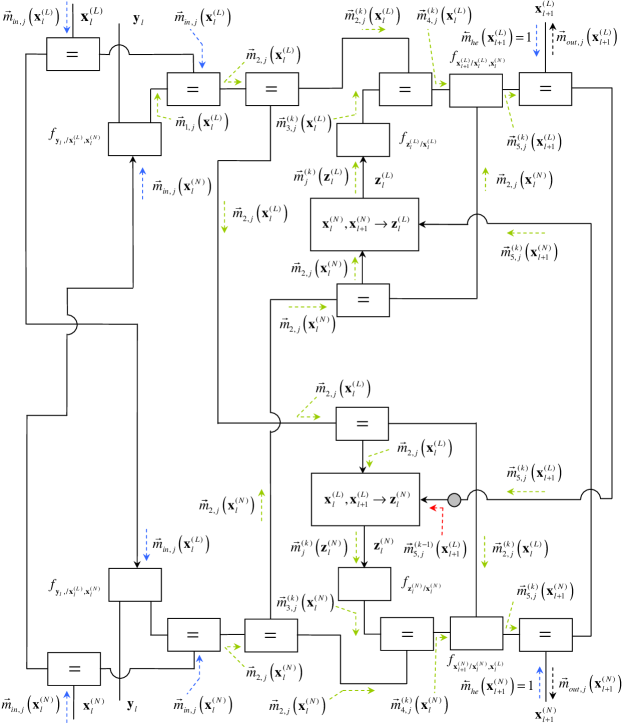
Figure 4: Message passing over the FG of Fig. 1 for the proposed TF technique. All the quantities appearing in this figure refer to the $k$-th iteration of the $l$-th recursion; the messages available at the beginning of the considered iteration are indicated by red arrows, those entering the graph by blue arrows, those leaving it at the end of the last iteration by black arrows and those computed within the considered iteration by green arrows.

Another relevant issue concerns the interpretation of the processing tasks accomplished in the TF technique. In fact, our derivations show that, at the end of the $k$-th iteration, the a posteriori statistical information about the $j$-th particle $\mathbf{x}_{l/l,j}^{(N)}[k]$ of $S_{l/l}^{(N)}[k]$ is provided by the message $\vec{m}_{4,j}^{(k)}(\mathbf{x}_{l}^{(N)})$ (97), which conveys the weight (see (98))

$$W_{l,j}[k]=w_{l,j}[k]\cdot p_{l,j}[k]\cdot w_{l,j}^{(a)},$$ (102)

where $w_{l,j}^{(a)}$ denotes the a priori information available at the beginning of the $l$-th recursion for the $j$-th particle ( in our derivation $w_{l,j}^{(a)}$ $=1$ has been assumed, in place of $w_{l,j}^{(a)}$ $=1/N_{p}$, to simplify the notation; see (22)), $p_{l,j}[k]$ is the weight originating from $\vec{m}_{j}(\mathbf{z}_{l}^{(N)})$ (87) and conveyed by $\vec{m}_{3,j}^{(k)}(\mathbf{x}_{l}^{(N)})$ (92), and $w_{l,j}[k]$ is the weight computed on the basis of the available measurement $\mathbf{y}_{l}$. Taking the natural logarithm of both sides of (102) produces

$$L_{l,j}[k]=L_{l,j}^{(a)}+L_{l,j}^{(y)}[k]+L_{l,j}^{(z)}[k],$$ (103)

where $L_{l,j}[k]\triangleq\ln(W_{l,j}[k])$, $L_{l,j}^{(y)}[k]\triangleq\ln(w_{l,j}[k])$, $L_{l,j}^{(z)}\triangleq\ln(p_{l,j}[k])$ and $L_{l,j}^{(a)}\triangleq\ln(w_{l,j}^{(a)})$. The last equation has exactly the same structure as the well known formula (see [35, Sec. 10.5, p. 450, eq. (19.15)] or [36, Par. II.C, p. 432, eq. (20)])

$$L\left(u_{j}|\mathbf{y}\right)=L\left(u_{j}\right)+L_{c}(y_{j})+L_{e}\left(u_{j}\right)$$ (104)

expressing of the log-likelihood ratio (LLR) available for the $j$-th information bit  $u_{j}$ at the output of a soft-input soft-output channel decoder operating over an additive white Gaussian noise (AWGN) channel and fed by: a) the channel output vector $\mathbf{y}$ (whose $j$-th element $y_{j}$ is generated by the communications channel in response to a channel symbol conveying $u_{j}$ and is processed to produce the so-called channel LLR $L_{c}(y_{j})$); b) the a priori LLR $L\left(u_{j}\right)$ about $u_{j}$; c) the extrinsic LLR $L_{e}\left(u_{j}\right)$, i.e. a form of soft information available about $u_{j}$, but intrinsically not influenced by such a bit (in turbo decoding of concatenated channel codes extrinsic infomation is generated by another channel decoder with which soft information is exchanged with the aim of progressively refining data estimates). This correspondence is not only formal, since in eqs. (103) and (104) terms playing similar roles can be easily identified. For instance, the term $L_{l,j}^{(y)}[k]$ ($L_{l,j}^{(a)}$) in (103) provides the same kind of information as $L_{c}(y_{j})$ ($L\left(u_{j}\right)$), since these are both related to the noisy data (a priori information) available about the quantities to be estimated (the system state in one case, an information bit the in the other one). What about the term $L_{l,j}^{(z)}[k]$ appearing in the RHS of (103)? The link we have established between (103) and (104) unavoidably leads to the conclusion that such a term should represent the counterpart of the quantity $L_{e}\left(u_{j}\right)$ appearing in (104), i.e. the so called extrinsic information (in other words, that part of the information available about $\mathbf{x}_{l}^{(N)}$ and not intrinsically influenced by $\mathbf{x}_{l}^{(N)}$ itself). This interpretation is confirmed by the fact that $L_{l,j}^{(z)}[k]$ is computed on the basis of the statistical knowledge available about $\mathbf{x}_{l}^{(L)}$ and $\mathbf{x}_{l+1}^{(L)}$ (see (88) and (90)), which, thanks to (2), does provide useful information about $\mathbf{x}_{l}^{(N)}$. The theory of turbo decoding of channel codes shows that, generally speaking, extrinsic information originates from code constraints. In our scenario, a similar interpretation can be also provided for $L_{l,j}^{(z)}[k]$, since $\mathbf{x}_{l+1}^{(L)}$ can be seen as the noisy output of a communication channel, affected by the bias $\mathbf{f}_{l,j}^{(L)}$ and the additive noise $\mathbf{w}_{l}^{(L)}$, and over which the codeword $\mathbf{A}_{l,j}^{(L)}\mathbf{x}_{l}^{(L)}$ of a rate-$1$ block code is transmitted in response to the message $\mathbf{x}_{l}^{(L)}$. These considerations show that, in evaluating $L_{l,j}^{(z)}[k]$, we are actually exploiting a sort of ‘code’ constraints, which are mathematically expressed by (2). The reader can easily verify that a similar interpretation can be provided for $\vec{m}_{j}(\mathbf{z}_{l}^{(L)})$ (53), which represents the extrinsic information component contained in $\vec{m}_{4,j}(\mathbf{x}_{l}^{(L)})$ (57) (conveying our a posteriori information about $\mathbf{x}_{l}^{(L)}$); the other two components are represented by the message $\vec{m}_{2,j}(\mathbf{x}_{l}^{(L)})$ (40) (representing the measurement information about $\mathbf{x}_{l}^{(L)}$) and the message $\vec{m}_{in,j}(\mathbf{x}_{l}^{(L)})$ (21) (corresponding to our a priori information about $\mathbf{x}_{l}^{(L)}$). Consequently, TF can be seen, in the domain of Bayesian filtering techniques, as the counterpart of turbo decoding of concatenated codes; this parallelism can be exploited to provide further insights into iterative filtering techniques. For instance, it is well known that, in turbo decoding of concatenated channel codes, the extrinsic information generated by soft decoders become more and more correlated as iterations evolve; this entails that diminishing benefits are provided by additional iterations. This phenomenon should be observed in TF too for similar reasons and can be motivated by rewriting $\mathbf{\eta}_{\mathbf{z},l,j}^{(N)}$ (88) and $\mathbf{C}_{\mathbf{z},l,j}^{(N)}$ (90) as

$$\mathbf{\eta}_{\mathbf{z},l,j}^{(N)}=\mathbf{f}_{l,j}^{(L)}+\mathbf{A}_{l,j}^{(L)}\left[\mathbf{\eta}_{4,l,j}^{(L)}-\mathbf{\eta}_{2,l,j}^{(L)}\right]$$ (105)

and

$$\mathbf{C}_{\mathbf{z},l,j}^{(N)}=\mathbf{C}_{w}^{(L)}+\mathbf{A}_{l,j}^{(L)}\left[\mathbf{C}_{4,l,j}^{(L)}-\mathbf{C}_{2,l,j}^{(L)}\right]\left(\mathbf{A}_{l,j}^{(L)}\right)^{T},$$ (106)

respectively (thanks to (85) and (86), respectively). In fact, the last two equations show that the vector $\mathbf{\eta}_{\mathbf{z},l,j}^{(N)}$ and the matrix $\mathbf{C}_{\mathbf{z},l,j}^{(N)}$ are influenced by the difference between the statistical information (expressed by a mean vector and a covariance matrix) available about $\mathbf{x}_{l}^{(L)}$ before processing the pseudomeasurement $\mathbf{z}_{l}^{(L)}$ and those available after this task has been carried out. In other words, the extrinsic information provided by $\mathbf{z}_{l}^{(L)}$ influences $\mathbf{z}_{l}^{(N)}$ and viceversa.

Finally, it is important to point out that the proposed analogy between turbo filtering and turbo decoding suggests the potential limits of the TF technique (and of any other iterative filtering method relying on the developed FG). In fact, it is well known that turbo decoding methods do not provide real benefits below a certain signal-to-noise ratio, i.e. when the quality of the received signal is so poor that the transmitted coded sequence cannot be recovered. A similar phenomenon is expected occur with TF too; consequently, this filtering method could not outperform MPF in the presence of strong measurement noise and/or fast dynamics affecting the considered SSM.

7 Numerical Results

In this Section MPF and the related filtering methods developed in this manuscript are compared in terms of accuracy and computational load for a specific CLG system, characterized by $D_{L}=3$, $D_{N}=1$ (so that $D=4$) and $P=2$. The structure of the considered system has been partly inspired by the example proposed by Schön in [37] and is characterized by: a) the state models

$$\mathbf{x}_{l+1}^{(L)}=\left(\begin{array}[c]{ccc}0.8&0.2&0\\ 0&0.7&-0.2\\ 0&0.2&0.7\end{array}\right)\mathbf{x}_{l}^{(L)}+\left(\begin{array}[c]{c}\cos(x_{l}^{(N)})\\ -\sin(x_{l}^{(N)})\\ 0.5\sin(2x_{l}^{(N)})\end{array}\right)+\mathbf{w}_{l}^{(L)}$$ (107)

and

$$x_{l+1}^{(N)}=\arctan\left(x_{l}^{(N)}\right)+\left(0.9\quad 0\quad 0\right)\mathbf{x}_{l}^{(L)}+w_{l}^{(N)}$$ (108)

with $\mathbf{w}_{l}^{(L)}\sim\mathcal{N}(0,(\sigma_{w}^{(L)})^{2}\mathbf{I}_{3})$, $w_{l}^{(N)}\sim\mathcal{N}(0,(\sigma_{w}^{(N)})^{2}$; b) the measurement model

$$\mathbf{y}_{l}=\left(\begin{array}[c]{c}0.1\left(x_{l}^{(N)}\right){}^{2}\cdot\text{sgn}\left(x_{l}^{(N)}\right)\\ 0\end{array}\right)+\left(\begin{array}[c]{ccc}0&0&0\\ 1&-1&1\end{array}\right)\mathbf{x}_{l}^{(L)}+\mathbf{e}_{l}$$ (109)

with $\mathbf{e}_{l}\sim\mathcal{N}(0,(\sigma_{e})^{2}\mathbf{I}_{2})$. Note that the state equation (107), unlike its counterpart proposed in [37], depends on $x_{l}^{(N)}$ (i.e., it contains a function $\mathbf{f}_{l}^{(L)}\left(x_{l+1}^{(N)}\right)\neq\mathbf{0}_{3}$ in its RHS), so that TF, which relies on the availability of the vector $\mathbf{z}_{l}^{(N)}$ (18), can be employed for this system.

In our computer simulations the root mean square error (RMSE) has been evaluated to compare the accuracy of the state estimates generated by different filtering techniques. More specifically, for each technique two RMSEs have been computed, one (denoted $RMSE_{L}($alg$)$, where ‘alg’ denotes the algorithm this parameter refers to) representing the square root of the average mean square error (MSE) evaluated for the three elements of $\mathbf{x}_{l}^{(L)}$, the other one (denoted $RMSE_{N}($alg$)$) referring to the (monodimensional) nonlinear component $x_{l}^{(N)}$; this distinction is important since, as shown by our simulation results, the estimation accuracy for $\mathbf{x}_{l}^{(L)}$ can be quite different from (and is usually smaller than) that referring to $x_{l}^{(N)}$.

As far the assessment of the computational requirements of the investigated filtering techniques is concerned, MPF (for which an accurate analysis of its computational complexity is available in [16]) has been taken as a baseline. For this reason, our comparisons between the considered filtering techniques are based on the evaluation of a single parameter, denoted $\Delta_{c}($alg$)$ and representing the percentage variation in computation time of the considered algorithm (denoted ‘alg’) with respect to MPF (operating with the same parameters and, in particular, with the same $N_{p}$ as alg).

Moreover, in our computer simulations, the following choices have been made: a) $\sigma_{w}^{(L)}=\sigma_{w}^{(N)}=5\cdot 10^{-3}$ has been selected for the standard deviations of the process noises $\{\mathbf{w}_{k}^{(L)}\}$ and $\{w_{k}^{(N)}\}$, unless differently stated; b) the so called jittering technique [34] has been employed to mitigate the so called depletion problem in the generation of new particles.

Some results illustrating the dependence of $RMSE_{L}$ and $RMSE_{N}$ on the number of particles ($N_{p}$) for MPF and SMPF#1 are illustrated in Fig. 5 (in this and in the following figures simulation results are identified by markers, whereas continuous lines are drawn to ease reading); $\sigma_{e}=10^{-2}$ and $N_{p}\in[50,300]$ have been selected in this case. From these results the following conclusions can be easily inferred for the considered system:

1. A negligible improvement in the estimation accuracy of both MPF and SMPF#1 is achieved if the value of $N_{p}$ exceeds $200$.

2. A significant gap between $RMSE_{L}($MPF$)$ and $RMSE_{N}($MPF$)$ exists; this is motivated by the fact that, in MPF, the estimation of $\mathbf{x}_{l}^{(L)}$ relies on both the real measurement $\mathbf{y}_{l}$ (109) and the pseudo-measurements $\{\mathbf{z}_{l,j}^{(L)}\}$ (54), whereas the estimation of $x_{l}^{(N)}$ benefits from $\mathbf{y}_{l}$ only.

3. The gap between $RMSE_{L}($SMPF#1$)$ and $RMSE_{N}($SMPF#1$)$ is much smaller than that observed for MPF, even if the pseudo-measurements $\{\mathbf{z}_{l,j}^{(L)}\}$ are also exploited by SMPF#1.  This reduction in the RMSE gap can be related to the degradation in the estimation accuracy of $\mathbf{x}_{l}^{(L)}$; for instance, for $N_{p}=200$, $RMSE_{L}($SMPF#1$)$ is about twice $RMSE_{L}($MPF$)$ (on the contrary, $RMSE_{N}($SMPF#1$)\cong 1.09\cdot$ $RMSE_{N}($MPF$)$).

Our numerical results have also evidenced that: a) SMPF#1 requires a substantially smaller computational effort than MPF, since $\Delta_{c}($SMPF#1$)$ approximately ranges in the interval $[-62\%,-58\%]\$ for the considered values of $N_{p}$; b) despite the above mentioned degradation in estimation accuracy (see point 3.), SMPF#1 does not suffer from tracking losses in the considered scenario; c) SMPF#2 accuracy is almost indentical that of SMPF#1; d) $\Delta_{c}($SMPF#2$)$ is approximately lower than $\Delta_{c}($SMPF#1$)$ by $6\%$ in the considered range for $N_{p}$ and, consequently, achieves a better complexity-performance tradeoff than SMPF#1. All this suggests that simplified MPF techniques can be really developed without incurring the serious technical problems that affect the techniques proposed in [17] (tracking losses and poor RMSE performance) and in [18] (partitioning and update of the particle set into groups within each recursion; see Section 5).

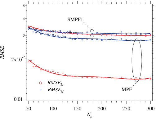
Figure 5: RMSE performance versus $N_{p}$ for the linear component ($RMSE_{L}$) and the nonlinear component ($RMSE_{N}$) of the state $\mathbf{x}_{l}$ for the system described by eqs. (107)-(109). MPF and SMPF#1 are considered; in both cases $\sigma_{w}^{(L)}=\sigma_{w}^{(N)}=5\cdot 10^{-3}$ and $\sigma_{e}=10^{-2}$ have been selected.

The dependence of $RMSE_{L}$ and $RMSE_{N}$ on $\sigma_{e}$ (i.e., on the intensity of the noise affecting the available measurements) has been also analysed for MPF and SMPF#1. Some results are shown in Fig. 6; $N_{p}$ $=500$ and $\sigma_{e}\in[10^{-3},5\cdot 10^{-2}]$ have been selected in this case. These results show that the gap between $RMSE_{L}($MPF$)$ and $RMSE_{L}($SMPF#1$)$ slightly increases as $\sigma_{e}$ becomes smaller; the opposite occurs for $RMSE_{N}($MPF$)$ and $RMSE_{N}($SMPF#1$)$. These results can be related again to the fact that the pseudo-measurements $\{\mathbf{z}_{l,j}^{(L)}\}$ (54) really play a role in the MPF estimation of $\mathbf{x}_{l}^{(L)}$ and that the quality of the information conveyed by these pseudo-measurements indirectly improves as the real measurements become less noisy.

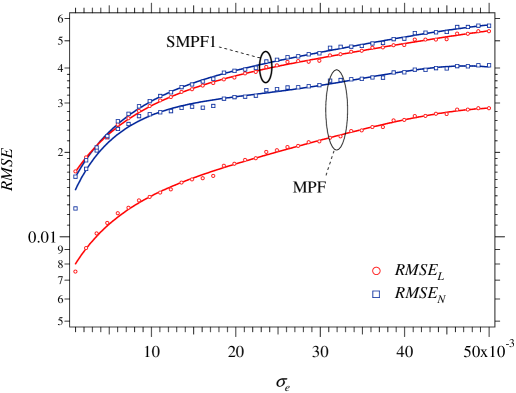
Figure 6: RMSE performance versus $\sigma_{e}$ for the linear component ($RMSE_{L}$) and the nonlinear component ($RMSE_{N}$) of the state $\mathbf{x}_{l}$ for the system described by eqs. (107)-(109). MPF and SMPF#1 are considered; in both cases $\sigma_{w}^{(L)}=\sigma_{w}^{(N)}=5\cdot 10^{-3}$ and $N_{p}=200$ have been selected.

Some results illustrating the dependence of $RMSE_{L}$ and $RMSE_{N}$ on the number of particles ($N_{p}$) for MPF and TF are illustrated in Fig. 7; $\sigma_{e}=10^{-2}$ , $N_{p}\in[1,300]$ and $N_{it}=2$ for TF, and $N_{p}\in[30,300]$ for MPF have been chosen in this case. From these results it is easily inferred that:

1. TF outperforms MPF in tems of both $RMSE_{L}$ and $RMSE_{N}$; for instance, $RMSE_{L}($MPF$)\cong 1.71\cdot$ $RMSE_{L}($TF$)$ and $RMSE_{N}($MPF$)\cong 2.86\cdot$ $RMSE_{N}($TF$)$ if $N_{p}=200$ is selected.

2. The gap between $RMSE_{L}($MPF$)$ and $RMSE_{N}($MPF$)$ is substantially larger than the corresponding gap for TF (in particular, $RMSE_{N}($MPF$)-RMSE_{L}($MPF$)$ $\cong 13.4\cdot[RMSE_{N}($TF$)-RMSE_{L}($TF$)]$; this can be easily related to the fact that, unlike MPF, in TF the estimation of both $\mathbf{x}_{l}^{(L)}$ and $x_{l}^{(N)}$ benefits from the availability of pseudo-measurements.

3. The performance gap between TF and MPF increases as $N_{p}$ gets smaller. Moreover, TF accuracy starts quickly degrading when $N_{p}$ drops below $11$, whereas the same phenomenon starts for $N_{p}\cong 30$ with MPF. Note, however, that different phenomena occur with MPF and TF when the particle set is small. In fact, our computer simulations have shown that MPF suffers from frequent tracking losses for $N_{p}<30$ (since it is unable to generate a reliable representation of $x_{l}^{(N)}$ when a limited number of particles is available); on the contrary, TF does not suffer from the same problem even if a very small particle set is used.

We believe that last result is really important and can be motivated as follows. The TF technique, through its feedback mechanism, makes a substantially more efficient use of the available particles than MPF; this results in an appreciable improvement of both stability and accuracy of state estimation.

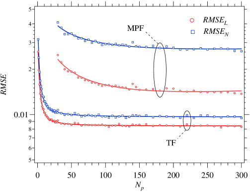
Figure 7: RMSE performance versus $N_{p}$ for the linear component ($RMSE_{L}$) and the nonlinear component ($RMSE_{N}$) of the state $\mathbf{x}_{l}$ for the system described by eqs. (107)-(109). MPF and TF are considered; in both cases $\sigma_{w}^{(L)}=\sigma_{w}^{(N)}=5\cdot 10^{-3}$ and $\sigma_{e}=10^{-2}$ have been selected.

Our simulation results have also shown that: a) in the considered scenario a negligible improvement in estimation accuracy is obtained if $N_{it}>2$ is selected; b) $\Delta_{c}($TF$)$ approximately ranges in the interval $[70\%,80\%]\$ for the considered values of $N_{p}$ and, consequently, requires a substantially larger computational effort than MPF if these algorithms operate with the same number of particles. In practice, however, as evidenced by the results shown in Fig. 7, TF can reliably operate with a very small particle set and, consequently, it outperforms MPF in terms of both performance and complexity if $N_{p}$ is properly selected. For instance, in the considered scenario TF with $N_{p}=20$ particles achieves a substally better accuracy than MPF with $N_{p}=40$ particles, even if, as evidenced by our computer simulations, they approximately require the same computation time. It is not difficult to show that similar considerations hold if SMPF#1 and SMPF#2 are considered in place of MPF. Therefore, our results suggest that the real key to the complexity reduction of the filtering techniques relying on the FG shown in Fig. 2 is not provided by the approximations adopted for the MPF processing tasks in Section 5, but by the exploitation of the new pseudo-measurement $\mathbf{z}_{l}^{(N)}$ (18). We should never forget, however, that TF cannot be adopted for all CLG systems; in fact, it cannot be employed if $\mathbf{f}_{l}^{(L)}\left(x_{l+1}^{(N)}\right)=\mathbf{0}_{D_{L}}$ in the RHS of (2).

Finally, the dependence of $RMSE_{L}$ and $RMSE_{N}$ on $\sigma_{e}$ has been assessed for TF and compared with that characterizing MPF. Some numerical are illustrated in Fig. 8. In this case, we have selected $\sigma_{e}\in[1.5\cdot 10^{-2},5\cdot 10^{-2}]$ , $N_{p}=200$ and $N_{it}=2$ for TF, and $N_{p}=200$ for MPF; moreover, $\sigma_{w}^{(L)}=\sigma_{w}^{(N)}=5\cdot 10^{-3}$ and $\sigma_{w}^{(L)}=\sigma_{w}^{(N)}=10^{-3}$ have been considered to analyse the dependence of the performance gap between TF and MPF on the intensity of process noise (and, consequently, on system dynamics). These results show that: a) the performance gap between TF and MPF undergoes small changes if $\sigma_{e}$ varies in the considered interval; b) on the contrary, a substantial change in this gap is obtained if $\sigma_{w}^{(L)}$ and $\sigma_{w}^{(N)}$ are reduced from $5\cdot 10^{-3}$ to $10^{-3}$. This suggests that measurement noise and process noise can have different impacts on the performance gain provided by TF over MPF.

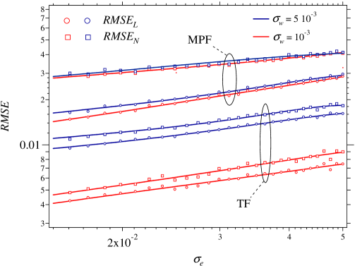
Figure 8: RMSE performance versus $\sigma_{e}$ for the linear component ($RMSE_{L}$) and the nonlinear component ($RMSE_{N}$) of the state $\mathbf{x}_{l}$ for the system described by eqs. (107)-(109). MPF and TF are considered; $\sigma_{e}=10^{-2}$ and $N_{p}=200$ are assumed in both cases. As far system noise is concerned, the cases $\sigma_{w}^{(L)}=\sigma_{w}^{(N)}=5\cdot 10^{-3}$ and $\sigma_{w}^{(L)}=\sigma_{w}^{(N)}=10^{-1}$ are taken into consideration.

8 Conclusions

In this manuscript a FG approach has been employed to analyse the filtering problem for mixed linear/nolinear models. This has allowed us to: a) prove that this problem involves a FG which is not cycle free; b) provide a new interpretation of MPF as a forward only message passing algorithm over a specific FG; c) develop novel filtering algorithms for simplifying or generalising it. In particular, an important iterative filtering technique, dubbed turbo filtering, has been devised and its relation with the turbo decoding techniques for concatenated channel codes has been analysed in detail. All the considered filtering techniques have been compared in terms of both accuracy and computational requirements for a specific CLG system. The most interesting result emerging from our computer simulations is represented by the clear superiority of turbo filtering over marginalized particle filtering. In fact, the former technique, through the exploitation of new pseudo-measurements, can achieve a better accuracy than the latter one at an appreciably smaller computational load. Our ongoing research activities in this area include the development of other related filtering techniques and the application of turbo filtering to specific state estimation problems.

Appendix A Appendix

Given the pdfs $f_{1}(\mathbf{y})\triangleq\mathcal{N}(\mathbf{y};\mathbf{\eta}_{1},\mathbf{C}_{1})$ and $f_{2}(\mathbf{y})\triangleq\mathcal{N}(\mathbf{y};\mathbf{\eta}_{1},\mathbf{C}_{2})$ for the $N$-dimensional vector $\mathbf{y}$, we are interested in evaluating the correlation between these two functions, i.e. the quantity

$$c_{1,2}\triangleq\int f_{1}(\mathbf{y})\cdot f_{2}(\mathbf{y})\,d\mathbf{y}$$ (110)

Substituting the expressions of $f_{1}(\mathbf{y})$ and $f_{2}(\mathbf{y})$ in the RHS of the last equation produces, after some manipulation,

$$c_{1,2}=D\,\exp\left[\frac{1}{2}\left(\mathbf{\eta}^{T}\mathbf{W}\mathbf{\eta}-\mathbf{\eta}_{1}^{T}\mathbf{W}_{1}\mathbf{\eta}_{1}-\mathbf{\eta}_{2}^{T}\mathbf{W}_{2}\mathbf{\eta}_{2}\right)\right]$$ (111)

where $\mathbf{\mathbf{W}}_{1}\triangleq\mathbf{C}_{1}^{-1}$, $\mathbf{\mathbf{W}}_{2}\triangleq\mathbf{C}_{2}^{-1}$,

$$\mathbf{W}=\mathbf{\mathbf{W}}_{1}+\mathbf{\mathbf{W}}_{2},$$ (112)

$$\mathbf{W}\mathbf{\eta}=\mathbf{W}_{1}\mathbf{\eta}_{1}+\mathbf{W}_{2}\mathbf{\eta}_{2}$$ (113)

and

$$D=\left(2\pi\det\left[\mathbf{C}_{1}+\mathbf{C}_{2}\right]\right)^{-N/2}.$$ (114)

References

- [1] M. S. Arulampalam, S. Maskell, N. Gordon and T. Clapp, “A Tutorial on Particle Filters for Online Nonlinear/Non-Gaussian Bayesian Tracking”, IEEE Trans. Sig. Proc., vol. 50, no. 2, pp. 174-188, Feb. 2002.
- [2] F. E. Daum, “Exact Finite-Dimensional Nonlinear Filters”, IEEE Tran. Aut. Contr., vol. 31, no. 7, pp. 616-622, July 1986.
- [3] S. Mazuelas, Y. Shen and M. Z. Win, “Belief Condensation Filtering”, IEEE Trans. Sig. Proc., vol. 61, no. 18, pp. 4403-4415, Sept. 2013.
- [4] V. Smidl and A. Quinn, “Variational Bayesian Filtering”, IEEE Trans. Sig. Proc., vol. 56, no. 10, pp. 5020-5030, Oct. 2008.
- [5] M. S̆imandl, J. Královeca and T. Söderströmc, “Advanced Point-Mass Method for Nonlinear State Estimation”, Automatica, vol. 42, pp. 1133-1145, 2006.
- [6] B. Anderson and J. Moore, Optimal Filtering, Englewood Cliffs, NJ, Prentice-Hall, 1979.
- [7] S. J. Julier and J. K. Uhlmann, “Unscented Filtering and Nonlinear Estimation”, IEEE Proc., vol. 92, no. 3, pp. 401-422, Mar. 2004.
- [8] A. Doucet, J. F. G. de Freitas and N. J. Gordon, “An Introduction to Sequential Monte Carlo methods,” in Sequential Monte Carlo Methods in Practice, A. Doucet, J. F. G. de Freitas, and N. J. Gordon, Eds. New York: Springer-Verlag, 2001.
- [9] A. Doucet, S. Godsill and C. Andrieu, “On Sequential Monte Carlo Sampling Methods for Bayesian Filtering”, Statist. Comput., vol. 10, no. 3, pp. 197-208, 2000.
- [10] F. Gustafsson, “Particle Filter Theory and Practice with Positioning Applications”, IEEE Aerosp. and Electr. Syst. Mag., vol. 25, no. 7, pp. 53-82, July 2010.
- [11] F. Gustafsson, F. Gunnarsson, N. Bergman, U. Forssell, J. Jansson, R. Karlsson and P. Nordlund, “Particle Filters for Positioning, Navigation, and Tracking”, IEEE Trans. Sig. Proc., vol. 50, 425-435, 2002.
- [12] P. J. Nordlund and F. Gustafsson, “Marginalized Particle Filter for Accurate and Reliable Terrain-Aided Navigation”, IEEE Trans. on Aerosp. and Elec. Syst., vol. 45, no. 4, pp. 1385-1399, Oct. 2009.
- [13] R. Bucy and K. Senne, “Digital Synthesis of Non-Linear Filters”, Automatica, vol. 7, no. 3, pp. 287-298, 1971.
- [14] F. Daum and J. Huang, “Curse of Dimensionality and Particle Filters”, Proc. IEEE Aerosp. Conf., vol. 4, pp. 1979-1993, March 2003.
- [15] T. Schön, F. Gustafsson, P.-J. Nordlund, “Marginalized Particle Filters for Mixed Linear/Nonlinear State-Space Models”, IEEE Trans. Sig. Proc., vol. 53, no. 7, pp. 2279-2289, July 2005.
- [16] R. Karlsson, T. Schön, F. Gustafsson, “Complexity Analysis of the Marginalized Particle Filter”, IEEE Trans. Sig. Proc., vol. 53, no. 11, pp. 4408-4411, Nov. 2005.
- [17] F. Mustiere, M. Bolic and M. Bouchard, “A Modified Rao-Blackwellised Particle Filter”, Proc. of the 2006 IEEE Int. Conf. on Ac., Sp. and Sig. Proc. (ICASSP 2006), vol. 3, 14-19 May 2006.
- [18] T. Lu, M. F. Bugallo and P. M. Djuric, “Simplified Marginalized Particle Filtering for Tracking Multimodal Posteriors”, Proc. IEEE/SP 14th Workshop on Stat. Sig. Proc. (SSP ’07), pp. 269-273, Madison, WI (USA), 2007.
- [19] F. Lindsten, P. Bunch, S. Särkkä, T. B. Schön and S. J. Godsill, “Rao-Blackwellized Particle Smoothers for Conditionally Linear Gaussian Models”, IEEE J. Sel. Topics in Sig. Proc., vol. 10, no. 2, pp. 353-365, March 2016.
- [20] H.-A. Loeliger, J. Dauwels, Junli Hu, S. Korl, Li Ping, F. R. Kschischang, “The Factor Graph Approach to Model-Based Signal Processing”, IEEE Proc., vol. 95, no. 6, pp. 1295-1322, June 2007.
- [21] F. R. Kschischang, B. Frey, and H. Loeliger, “Factor Graphs and the Sum-Product Algorithm”, IEEE Trans. Inf. Theory, vol. 41, no. 2, pp. 498-519, Feb. 2001.
- [22] C. Berrou and A. Glavieux, “Near Optimum Error Correcting Coding and Decoding: Turbo-Codes”, IEEE Trans. Commun., vol. 44, no. 10, pp. 1261 - 1271, Oct. 1996.
- [23] S. Benedetto, D. Divsalar, G. Montorsi and F. Pollara, “Serial Concatenation of Interleaved Codes: Performance Analysis, Design, and Iterative Decoding”, IEEE Trans. Inf. Theory, vol. 44, no. 3, pp. 909-926, May 1998.
- [24] R. Koetter, A. C. Singer and M. Tüchler, “Turbo Equalization”, IEEE Sig. Proc. Mag., vol. 21, no. 1, pp. 67-80, Jan. 2004.
- [25] J. Hagenauer, “The Turbo Principle: Tutorial Introduction & State of the Art”, Proc. Int. Symp. Turbo Codes & Related Topics, Brest, France, Sep. 1997, pp. 1-11.
- [26] A. P. Worthen and W. E. Stark, “Unified Design of Iterative Receivers using Factor Graphs”, IEEE Trans. Inf. Theory, vol. 47, no. 2, pp. 843–849, Feb. 2001.
- [27] F. R. Kschischang and B. J. Frey, “Iterative Decoding of Compound Codes by Probability Propagation in Graphical Models”, IEEE J. Sel. Areas Commun., vol. 16, no. 2, pp. 219-230, Feb. 1998.
- [28] J. Dauwels, S. Korl and H.-A. Loeliger, “Particle Methods as Message Passing”, Proc. 2006 IEEE Int. Symp. on Inf. Theory, pp. 2052-2056, 9-14 July 2006.
- [29] T. P. Minka, “Expectation Propagation for Approximate Bayesian Inference”, Proc. 17th Annual Conf. Uncertainty in Artif. Intell., pp. 362-369, Seattle, WA (USA), Aug. 2001.
- [30] O. Zoeter and T. Heskes, “Deterministic Approximate Inference Techniques for Conditionally Gaussian State Space Models”, Statistics and Computing, vol. 16, no. 3, pp. 279-292, Sep. 2006.
- [31] V. Smídl and A. Quinn, The Variational Bayes Method in Signal Processing, Berlin, Germany, Springer, 2005.
- [32] C. M. Bishop, Pattern Recognition and Machine Learning, Springer, 2006.
- [33] A. R. Runnalls, “Kullback-Leibler Approach to Gaussian Mixture Reduction”, IEEE Trans. on Aer. and Elec. Syst., vol. 43, no. 3, pp. 989-999, July 2007.
- [34] T. Li, M. Bolic, P. Djuric, “Resampling Methods for Particle Filtering: Classification, Implementation, and Strategies”, IEEE Sig. Proc. Mag., vol. 32, no. 3, pp.70-86, May 2015.
- [35] G. M. Vitetta, D. P. Taylor, G. Colavolpe, F. Pancaldi and P. A. Martin, Wireless Communications: Algorithmic Techniques, John Wiley & Sons, 2013.
- [36] J. Hagenauer, E. Offer and L. Papke, “Iterative decoding of binary block and convolutional codes”, IEEE Trans. Inf. Theory, vol. 42, no. 2, pp. 429-445, Mar 1996.
- [37] T. Schön, “Example Used in Exemplifying the Marginalized (Rao-Blackwellized) Particle Filter”, Nov. 2010 (available at http://users.isy.liu.se/en/rt/schon/Code/RBPF/Document/MPFexample.pdf).