Temperature chaos is a non-local effect

Abstract

Temperature chaos plays a role in important effects, like for example memory and rejuvenation, in spin glasses, colloids, polymers. We numerically investigate temperature chaos in spin glasses, exploiting its recent characterization as a rare-event driven phenomenon. The peculiarities of the transformation from periodic to anti-periodic boundary conditions in spin glasses allow us to conclude that temperature chaos is non-local: no bounded region of the system causes it. We precise the statistical relationship between temperature chaos and the free-energy changes upon varying boundary conditions.

1 Introduction.

Temperature chaos [1, 2, 3, 4, 5, 6, 7, 8, 9, 10, 11, 12, 13], is one of the outstanding mysteries posed by spin glasses [14, 15, 16, 17, 18, 19, 20]. It consists in the complete reorganization of the equilibrium configurations by the slightest change in temperature. The topic is currently under intense theoretical scrutiny [21, 22, 23, 24], not only because of its importance to analyze spectacular experiments [25, 26, 27, 28, 29, 30, 31, 32], but also as a crucial tool to assess the performance of quantum annealers [33, 34].

Here we exploit some of its very peculiar features to show that temperature chaos is a spatially non-local effect. For a disordered system, chaos should be studied on a sample by sample basis. In particular, for system sizes accessible to equilibrium computer simulations, chaos is a rare event, present only in a small fraction of the samples (as the system size increases, so does the fraction of chaotic samples [22]). We use this fact by thermalizing spin glasses down to a very low temperature (well below the critical temperature $T_{\mathrm{c}}$). Then, for each simulated system, with periodic boundary conditions (PBC), we consider its image under a transformation where we make the boundary conditions anti-periodic (APBC) in one direction. As we discuss below, this transformation amounts to change a tiny fraction of the coupling constants. Now, due to the gauge invariance in spin glasses, the couplings that have been changed by our transformation can be placed anywhere in the lattice. Interestingly enough, whether or not the PBC instance is chaotic carries essentially no information on the behaviour of its APBC transform. It follows that temperature chaos is not encoded in any localized region of the system.

We remark that our work relates as well to the long-standing controversy regarding the nature of the spin-glass phase. On the one hand, the Replica Symmetry Breaking theory (stemming from the mean-field solution) envisages the spin-glass phase as composed of a multiplicity of states [16, 35]. Thus, from this point of view, the change of boundary conditions is a strong perturbation and there are no reasons to expect that temperature chaos effects will be significantly correlated for the PBC system and its APBC transform. On the other hand, the droplet picture [36, 37, 38, 39] expects a single domain wall difference between the two types of boundary conditions, so there would be a strong correlation of the temperature chaos effects for the PBC/APBC systems. In this respect, our data favour Replica Symmetry Breaking (because little correlation is observed). However, it has been pointed out many times that resolving this controversy requires studying much larger systems than it is accessible to current simulations (or experiments [40]). This work is no exception. Furthermore, our analysis relies crucially in that the system sizes are modest. Indeed, we rely in that temperature chaos is a rare-event on small systems while, for larger systems, one expects that typical samples will display strong chaotic events.

The layout of the remaining part of this paper is as follows. In Sect. 2 we recall the model definition and the crucial quantities we study. Some crucial features of temperature chaos are presented in Sect. 3. Our main results are given in Sect. 4. We briefly explore the relationships between the free-energy and temperature chaos in Sect. 5. Our conclusions are given in Sect. 6. Technical details are provided in two appendices.

2 The Edwards-Anderson model.

Our $S_{\boldsymbol{u}}=\pm 1$ spins occupy the nodes of a $D=3$ lattice of size $L^{3}$ endowed with periodic boundary conditions. The Hamiltonian is

$$\mathcal{H}=-\sum_{\langle\boldsymbol{u},\boldsymbol{v}\rangle}S_{\boldsymbol{u}}J_{\boldsymbol{u}\boldsymbol{v}}S_{\boldsymbol{v}}\,.$$ (1)

The couplings $J_{\boldsymbol{u},\boldsymbol{v}}$ are $\pm 1$ with $50\%$ probability and only connect nearest neighbouring sites on the lattice. A particular realization of these couplings (quenched, i.e., fixed once and for all) is called a sample. Thermal averages for fixed $\{J_{\boldsymbol{u},\boldsymbol{v}}\}$ are denoted by $\langle\cdots\rangle_{J}$. This system has a second-order phase transition at temperature $T_{\mathrm{c}}=1.102(3)$ [41].

For any original (periodic, PBC) instance its anti-periodic pair (APBC) is obtained by reversing the coupling $J_{\boldsymbol{u},\boldsymbol{v}}$ that join sites $(x=0,y,z)$ and $(1,y,z)$ for all values of $y$ and $z$ [only a $1/(3L)$ fraction of the bonds is changed ]. The APBC image could be a perfectly reasonable original instance, and, in fact, it is as probable as its PBC pair.

Figure 1: Signatures of temperature chaos. Top: for a strongly chaotic (A, circles) and a non-chaotic (B, squares) sample, we show the chaos parameter $X_{T_{\mathrm{min}}=0.479,T}$ (solid symbols) and the energy per bond $\langle H/(3L^{3})\rangle_{J}$ (empty symbols) as a function of temperature. The dotted vertical line marks the critical temperature. A chaotic event for sample A at $T\approx 0.65$ is signalled by the strong drop of $X$. On the other hand, the effect in the energy is very subtle. Bottom: Probability distribution of the chaos integral $I_{J}$, as computed for lattices $L=8,12$ and $16$, with $T_{\mathrm{min}}=0.479$ and $T_{\mathrm{max}}=1.6$ (for all $L$, the same set of temperatures was used in the parallel tempering simulations). The distributions obtained with PBC and APBC are, of course, identical. The fraction of chaotic samples (i.e., small $I$) increases with system size. $L=16$ data from Ref. [40].

The system described by Eq. (1) has a gauge invariance [43]. The energy remains unchanged under the following transformation:

$$J_{\boldsymbol{u},\boldsymbol{v}}\longrightarrow\epsilon_{\boldsymbol{u}}\epsilon_{\boldsymbol{v}}J_{\boldsymbol{u},\boldsymbol{v}}\,,\quad S_{\boldsymbol{u}}\longrightarrow\epsilon_{\boldsymbol{u}}S_{\boldsymbol{u}}\;,$$ (2)

where $\epsilon_{\boldsymbol{u}}=\pm 1$ can be chosen arbitrarily for each site $\boldsymbol{u}$. Now consider the transformation where $\epsilon_{(1,y,z)}=-1$ and all other $\epsilon_{\boldsymbol{u}}=1$. This changes only the $J_{\boldsymbol{u},\boldsymbol{v}}$ that were reversed by the APBC transformation and those joining planes $x=1$ and $x=2$, moving in this way the transformed-couplings plane from $x=0$ to $x=1$. Using the same idea, we can place the transformed plane at any $x$. Furthermore, one can deform the plane of inverted couplings locally in an essentially arbitrary way by considering a more complicated gauge transformation. In short, the PBC $\leftrightarrow$ APBC transformation is non-local.

Another consequence of this gauge symmetry is the need to use real replicas of the system (i.e., copies that evolve independently but share the same couplings) in order to form gauge-invariant observables (see, e.g., [40]).

Figure 2: The non-local nature of chaos. Scatter plot of the chaos integral $(I_{\mathrm{PBC}},I_{\mathrm{APBC}})$ as computed for each of our 4000 pairs of samples with $L=12$ and $T_{\mathrm{min}}=0.414$. Hereafter we shall only show data from this simulation (the qualitatively identical results for other values of $L$ and $T_{\mathrm{min}}$ can be found in C).

We have simulated system sizes $L=8,12$ with parallel tempering [44, 45], carrying out several sets of runs for varying minimum temperature: $T_{\mathrm{min}}=0.15,0.414,0.479$ for $L=8$ and $T_{\mathrm{min}}=0.414,0.479$ for $L=12$. We have studied the same $4000$ samples and their $4000$ APBC counterparts for all $T_{\mathrm{min}}$. Since we want to study single-sample quantities and chaos, it has been very important to assess thermalization sample by sample by studying the temperature-mixing auto-correlation time of the parallel tempering [46]. In particular, we use the thermalization criteria of [40] (see also A).

3 Some crucial facts about temperature chaos.

Recently there has been much progress in the numerical characterization of temperature chaos [22, 23, 33]. A distinguishing feature of a chaotic sample is a very long auto-correlation time $\tau$ for temperature-mixing along a parallel tempering simulation. Unfortunately, $\tau$ is very difficult to measure with any precision, even for well equilibrated systems [40]. As shown in [22], see also B, this difficulty can be skirted by choosing a different quantity, easier to measure but strongly correlated with $\tau$.

In particular, we study the overlap between the spin configurations at temperatures $T_{1}$ and $T_{2}$,

$$q_{T_{1},T_{2}}=\frac{1}{L^{3}}\sum_{\boldsymbol{u}}q_{\boldsymbol{u}}^{T_{1},T_{2}}\,,\quad\mathrm{with}\quad q_{\boldsymbol{u}}^{T_{1},T_{2}}=S_{\boldsymbol{u}}^{T_{1}}S_{\boldsymbol{u}}^{T_{2}}\,,$$ (3)

and use it to define a chaos parameter [47]:

$$X_{T_{1},T_{2}} =\left\langle{q^{2}_{T_{1},T_{2}}}\right\rangle_{J}\big{/}\big{(}\left\langle{q^{2}_{T_{1},T_{1}}}\right\rangle_{J}\left\langle{q^{2}_{T_{2},T_{2}}}\right\rangle_{J}\big{)}^{1/2}\,,$$ (4)

$$I =\sum_{T_{2}}X_{T_{\mathrm{min}},T_{2}}\,.$$ (5)

In these equations, $\{S^{T_{1}}\}$ and $\{S^{T_{2}}\}$ are extracted from different real replicas. $X_{T_{1},T_{2}}$ is small when the equilibrium configurations at $T_{1}$ and $T_{2}$ differ significantly. Instead, $X_{T_{1},T_{2}}\approx 1$ in the absence of temperature chaos.

Figure 3: Absence of correlations. The red histogram is the probability density function of the chaos integral $p(I)$ for our PBC samples ($L=12$, $T_{\mathrm{min}}=0.414$). Now, let us consider the typical samples, namely those spanning the $20\%$ probability range around the median (the third quintile, if we divide the population in fifths). These third quintile samples belong to the narrow $I$ interval bounded by the two vertical green lines. Since temperature chaos is still rare for this system size, the third quintile samples are not chaotic. However, their APBC transforms (blue histogram) span the whole $I$ interval and reproduce the $p(I)$ for PBC. Indeed, an Anderson-Darling non-parametric test [48] yields a $p$-value of $53\%$ for the equal-distribution hypothesis. Inset: had we selected the $20\%$ most chaotic PBC instances (first quintile) the $p(I)$ for their APBC images would be slightly but definitively biased towards small $I_{J}$ (Anderson-Darling $p$-value of $0.08\%$). Indeed, the inset shows the conditional probability of having $I_{APBC}$ in the $k$-th quintile, given a fixed PBC quintile. For the central PBC quintile, the APBC conditional probability is uniform. For the first PBC quintile the APBC conditional probability is very slightly weighted to small $I$.

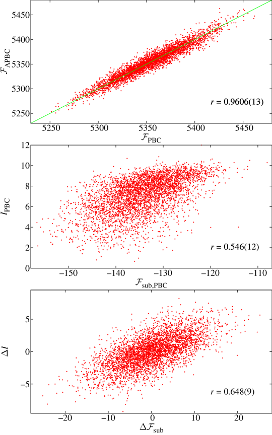
Figure 4: Temperature chaos and the free energy. We show several scatter plots for our $L=12$ and $T_{\mathrm{min}}=0.414$ data. Top: For the free-energy (6) we plot $({\cal F}_{\mathrm{PBC}},{\cal F}_{\mathrm{APBC}})$ for each of our 4000 sample pairs. The green straight line is $y=x$. Center: For the subtracted free-energy (7) we plot $({\cal F}_{\mathrm{sub,PBC}},I_{\mathrm{PBC}})$. Bottom: we plot $({\cal F}_{\mathrm{sub,PBC}}-{\cal F}_{\mathrm{sub,APBC}},I_{\mathrm{PBC}}-I_{\mathrm{APBC}})$.

We illustrate the ideas behind these parameters in Figure 1—top, where we represent $X_{T_{\mathrm{min}},T_{2}}$ for two samples $A$ and $B$. The ratio of their respective temperature-mixing times is $\tau^{\mathrm{A}}/\tau^{\mathrm{B}}\approx 3000$. Consequently, for sample A we can appreciate a very sudden drop in $X_{T_{\mathrm{min}},T_{2}}$ (which we name a chaotic event) for a low value of $T_{2}$, while sample B has a smooth $X$. This behaviour can be summarized by saying that chaotic samples (such as A) have a low value of $I$ (essentially the integral of $X$), while non-chaotic samples have a high $I$. Figure 1—bottom shows that the probability of finding a chaotic event in a prefixed temperature interval increases for larger system size .

We note also from Figure 1—top that the energy relates only in a very subtle way with temperature chaos. We shall further explore this relation below, since this quantity has been much emphasized in the literature [49, 12, 13, 24].

Finally, let us mention that we will base our analysis on $I$. However, essentially identical results are obtained from the temperature-mixing time $\tau$, as shown in B.

4 Results.

As Fig. 2 shows, the chaos integral $I$ for a sample has very low correlation to the $I$ value for its APBC transform. Yet, the $I$’s are not normally distributed (because the shape of the scatter plot is not elliptical). As a consequence, the characterization of correlations through the very small correlation parameter $r=0.074(16)$ is not complete. However, we can confirm the virtual absence of correlations is confirmed by a more refined analysis.

We start by considering the full probability distribution of $I$ for our PBC samples, which spans a wide range of values and of course coincides with the $p(I)$ for all the APBC samples. We then take the most typical samples, those contained in an interval of 20% probability around the median (the third quintile). All these samples, which span a very narrow $I$ range, are non-chaotic. If we consider the APBC transforms of this median samples at a first glance one can observe that they span the whole $I$ and therefore contain also chaotic instances. More precisely, one can construct the histogram of $I$ values for the APBC images of the PBC median, which turns out to reproduce exactly the full probability distribution of $I$ for this system. This is graphically shown in Fig. 3 but it can be proven using statistical methods. In particular, an Anderson-Darling non-parametric test [48] finds no difference between the full probability distribution of $I$ for the $L=12,T_{\mathrm{min}}=0.414$ system and the probability distribution of the images of the (non-chaotic) PBC median.

In short, the $I$ value of the APBC image of a median sample is completely uncorrelated with its $I_{\mathrm{PBC}}$. If we repeat the same analysis, using not the median PBC samples but the 20% most chaotic ones (the first quintile in $I$) we would find that again the APBC images span the whole $I$ range but now with a small bias toward low $I$ (see inset to Fig. 3). This is the reason for the non-Gaussian behaviour observed in Fig. 2.

Note that Figs. 2 and 3 are obtained from only one of our sets of simulations, but our results are essentially $L$- and $T_{\mathrm{min}}$-independent (see C).

5 Free energy and temperature chaos.

The free-energy change upon varying boundary conditions, $\Delta F=F_{\mathrm{APBC}}-F_{\mathrm{PBC}}$, has received much attention [49, 12, 13, 24]. However, to the best of our knowledge, the relation between $\Delta F$ and the spin correlations [e.g., the chaos parameter $X$ (4)], is yet to be researched. We can investigate $\Delta F$ from our parallel tempering simulations by means of thermodynamic integration:

$${\cal F}=\frac{F(T_{\mathrm{min}})}{T_{\mathrm{min}}}-\frac{F(T_{\mathrm{max}})}{T_{\mathrm{max}}}=\int_{T_{\mathrm{min}}}^{T_{\mathrm{max}}}\mathrm{d}\,T\,\frac{\langle H\rangle_{J,T}}{T^{2}}\,.$$ (6)

Here, $T_{\mathrm{max}}=1.6$ is the maximum temperature in our parallel tempering simulation. Note that, for large enough $T_{\mathrm{max}}$, $\Delta{\cal F}=\Delta F/T_{\mathrm{min}}$. Indeed, for a temperature $T$ such that the high-temperature expansion converges [50], $\Delta F(T)$ goes to zero exponentially in $L$.

Figure 1—top shows that chaotic events have an impact, albeit subtle, on the temperature evolution of $\langle H\rangle_{J,T}$. Hence, we expect some correlation between $X$ and the free energy. The question we address here is: how can we extract these correlations?

First, we note that $\mathcal{F}$ is not a good chaos indicator by itself. This is clear already from Fig. 1, but can be be seen more explicitly in Figure 4—top, where we show that $\mathcal{F}_{\mathrm{PBC}}$ and $\mathcal{F}_{\mathrm{APBC}}$ are almost equal (their correlation parameter is about $r\approx 0.95$). However, on a closer inspection one realizes that chaotic events, even close to $T=0$, result in minimal energy changes [51]. In other words, even in the most favourable case where only one member of the (PBC, APBC) pair has a chaotic event, the energy difference between the two samples is very small. Therefore, some sort of background subtraction is needed to enhance the chaotic signal:

$${\cal F}_{\mathrm{sub}}=\int_{T_{\mathrm{max}}}^{T_{\mathrm{min}}}\mathrm{d}\,T\,\frac{\langle H\rangle_{J,T}-\langle H\rangle_{J,T_{\mathrm{min}}}}{T^{2}}$$ (7)

Notice that, at very low temperature, (7) highlights the entropic contribution.

As we in see Figure 4—centre, $\mathcal{F}_{\mathrm{sub}}$ is correlated with the chaos integral $I$. However, this correlation is only of $r=0.546(12)$ and the scatter plot has a non-trivial structure, seemingly composed of two different populations. Therefore, $\mathcal{F}_{\mathrm{sub}}$, by itself, still does not seem a very good indicator of temperature chaos.

It is important to notice that the very strong correlation of $(\mathcal{F}_{\mathrm{PBC}},\mathcal{F}_{\mathrm{APBC}})$, together with the (weaker) correlation of $(\mathcal{F}_{\mathrm{PBC}},I_{\mathrm{PBC}})$ is in no contradiction with our previous assertion that $(I_{\mathrm{PBC}},I_{\mathrm{APBC}})$ are uncorrelated.

In order to see why, let us consider two stochastic variables, $A$ and $B$, that have the same variance $V$ and covariance $C$. Their covariance matrix has eigenvalues $\lambda_{\pm}=V\pm C$, and the corresponding normal coordinates are $N_{\pm}=(A\pm B)/\sqrt{2}$. It follows that the correlation coefficient is

$$r=\frac{C}{V}=\frac{1-\frac{\lambda_{-}}{\lambda_{+}}}{1+\frac{\lambda_{-}}{\lambda_{+}}}\,.$$ (8)

Clearly, $F_{\mathrm{APBC}}$ and $F_{\mathrm{PBC}}$, play the role of the stochastic variables $A$ and $B$ in the above reasoning. Now, as we shall explain next, there is a physical reason implying that $\lambda_{+}$ is orders of magnitude larger than $\lambda_{-}$. It follows that the correlation coefficient is $r\approx 1$ (as we find indeed). In other words, the only information in Fig. 4-top is $\lambda_{+}\gg\lambda_{-}$.

The physical reason underlying $\lambda_{+}\gg\lambda_{-}$ is quite simple. On the one hand the sample to sample fluctuations of the free-energy are of order $L^{D/2}$. On the other hand, $\lambda_{-}$, which is the variance of $(\mathcal{F}_{\mathrm{APBC}}-\mathcal{F}_{\mathrm{PBC}})/\sqrt{2}$ scales with the so called stiffness exponent $\lambda_{-}\propto L^{2y}$ with $y\approx 0.24$ in $D=3$ [52]. An elementary computation tells us that $\lambda_{-}/\lambda_{+}\propto L^{-x}$ with $x=D-2y\approx 2$.

A consequence of this analysis is that the free-energy difference $\Delta\mathcal{F}_{\mathrm{sub}}=(\mathcal{F}_{\mathrm{sub,APBC}}-\mathcal{F}_{\mathrm{sub,PBC}})$ is probably a much better chaos indicator than $\mathcal{F}_{\mathrm{sub}}$ by itself. This is confirmed by Figure 4—bottom, which shows an enhanced correlation between $\Delta\mathcal{F}_{\mathrm{sub}}$ and $\Delta I$, with a more Gaussian behaviour.

In conclusion, the free energy is related to temperature chaos as studied from the spatial correlation functions, but its sample-to-sample fluctuations are affected by several factors not related to chaos (see D). Therefore, a refined analysis is needed to extract information about the chaos integrals from $F$.

6 Conclusions.

We have shown that temperature chaos, one of the most complex effects in glass physics, is a non-local phenomenon. Our approach has two fundamental ingredients: the recent rare-event characterization of chaos and the very special nature of periodic boundary conditions transformations in disordered systems. In fact, anti-periodic boundary conditions cannot be precisely located in a finite region of the system. So, changing a tiny [$\mathcal{O}(1/L)$] fraction of the coupling constants produces a dramatic effect in the physics of the considered sample (and the spatial location of the changed couplings has little importance).

Appendix A Simulation parameters

Table 1: Parameters of our parallel-tempering simulations. In all cases we have simulated four independent real replicas for each of our $4000$ samples. The $N_{T}$ temperatures are uniformly distributed between $T_{\mathrm{min}}$ and $T_{\mathrm{max}}$. In this table $N_{\mathrm{mes}}$ is the number of heat-bath sweeps between measurements (we perform one parallel-tempering update every 10 heat-bath sweeps). The simulation length was adapted to the thermalization time of each sample (see [40]). The table shows the minimum, maximum and medium simulation times ($N_{\mathrm{HB}}$) for each lattice, in heat-bath steps.

$L$	$T_{\mathrm{min}}$	$T_{\mathrm{max}}$	$N_{T}$	$N_{\mathrm{mes}}$	$N_{\mathrm{HB}}^{\mathrm{min}}$	$N_{\mathrm{HB}}^{\mathrm{max}}$	$N_{\mathrm{HB}}^{\mathrm{med}}$
8	0.150	1.575	10	$10^{3}$	$5\times 10^{6}$	$8.30\times 10^{8}$	$7.82\times 10^{6}$
8	0.414	1.554	10	$10^{3}$	$10^{7}$	$2.00\times 10^{7}$	$1.00\times 10^{7}$
8	0.479	1.619	7	$10^{3}$	$10^{7}$	$10^{7}$	$10^{7}$
8	0.479	1.575	16	$10^{3}$	$10^{7}$	$10^{7}$	$10^{7}$
12	0.414	1.575	12	$5\times 10^{3}$	$10^{7}$	$1.53\times 10^{10}$	$4.60\times 10^{7}$
12	0.479	1.640	12	$2\times 10^{3}$	$8\times 10^{6}$	$7.49\times 10^{8}$	$1.08\times 10^{7}$
12	0.479	1.575	16	$2\times 10^{3}$	$8\times 10^{6}$	$2.56\times 10^{9}$	$1.94\times 10^{7}$

Our parallel tempering simulations closely follow Ref. [40]. Some details are provided in Table 1 for the sake of completeness. There are two simulation phases. In the first phase, all the PBC instances (and their APBC images) are simulated for the same amount of time (which is referred to in Table 1 as the minimum simulation time $N_{\mathrm{HB}}^{\mathrm{min}}$). At that point, we attempt a first estimate of the temperature-mixing time $\tau$ for each instance and check that the thermalization criteria were met [40]. We chose $N_{\mathrm{HB}}^{\mathrm{min}}$ in such a way that most instances (at least a $2/3$ fraction) are well thermalized. For the remaining instances, the simulation length is increased and $\tau$ recomputed. The procedure follows until safe thermalization is achieved.

Some of the simulations for our PBC-samples were actually taken from Ref. [40], specifically the $(L=8,T_{\mathrm{min}}=0.15)$ and $(L=12,T_{\mathrm{min}}=0.414)$ simulations. We did perform totally new simulations for the APBC image of this system. Additional simulations were performed in order to show the size-dependence in Fig. 1—bottom (the comparison of the chaos integral is easiest if we employ the same temperature grid in the Parallel Tempering for all system sizes).

Appendix B Mixing time or chaos integral?

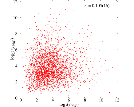
Figure 5: The chaos integral and the temperature-mixing autocorrelation time carry similar information. We show here two scatter plots, obtained from our $L=12$, $T_{\mathrm{min}}=0.414$ data. Left: We plot $(\mathrm{log}_{2}(\mathrm{PBC}),I_{PBC})$ for each of our 4000 original PBC samples. Right: for the temperature-mixing time $\tau$, we plot $(\mathrm{log}_{2}(\mathrm{PBC}),\mathrm{log}_{2}(\mathrm{APBC}))$ for each of our 4000 sample pairs. All the $\tau$ are integrated autocorrelation times (see [40]) and are expressed in units of $N_{\mathrm{mes}}=5000$ heat-bath steps (see Table 1).

As we explained in Sect. 3 the most appealing numerical characterization of temperature is the auto-correlation time $\tau$ for temperature-mixing along a parallel tempering simulation [22, 33]. Unfortunately, a high-accuracy computation of $\tau$ is not a light task, so we need an easier-to-compute alternative. A nice alternative is provided by the chaos integral $I$ defined in Eq. (5) [22].

Indeed, see Fig. 5—left, our estimations of $\tau$ and $I$ are very strongly correlated. Furthermore, our main theme (namely the very small correlation between the original PBC sample and its APBC-transform) is maintained when we work in terms of $\tau$, see Fig. 5—right.

Appendix C Additional results

The purpose of this section is to show that neither the choice of temperature interval nor of studied system size is critical. This is evinced in Figs. 6, 7 and 8.

Figure 6: We show two scatter plots, as obtained from our $L=8$ and $T_{\mathrm{min}}=0.15$ data. Left: The analogous of Fig. 5—left. Right: The analogous of Fig. 2.

Figure 7: The analogous of Fig 3, as obtained from our $L=8$ and $T_{\mathrm{min}}=0.15$ data.

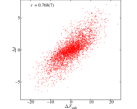
Figure 8: We show two scatter plots for our $L=8$ and $T_{\mathrm{min}}=0.15$ data (this figure is the analogous of Fig 4, as obtained for these $L$ and $T_{\mathrm{min}}$). Left: For the free-energy (6) we plot $({\cal F}_{\mathrm{PBC}},{\cal F}_{\mathrm{APBC}})$ for each of our 4000 sample pairs. The green straight line is $y=x$. Right: we plot $({\cal F}_{\mathrm{sub,PBC}}-{\cal F}_{\mathrm{sub,APBC}},I_{\mathrm{PBC}}-I_{\mathrm{APBC}})$.

Appendix D A geometric inequality on correlations

The assertion that the pair of stochastic variables $(I_{\mathrm{APBC}},I_{\mathrm{PBC}})$ are essentially uncorrelated might be surprising on the view of the mild correlations for $({\cal F}_{\mathrm{PBC}},I_{\mathrm{PBC}})$ [or, equivalently, $({\cal F}_{\mathrm{APBC}},I_{\mathrm{APBC}})$] and the very strong correlations depicted in Fig. 4 for $({\cal F}_{\mathrm{APBC}},{\cal F}_{\mathrm{PBC}})$. A simple geometric argument explains how misleading this way of reasoning might be. We thank one of our referees for calling our attention to this issue.

We shall first obtain an inequality, and then apply it to our problem. We start by considering a triplet of stochastic variables $(X_{0},X_{1},X_{2})$. Let $E(\cdots)$ denote the expectation value. For each $X_{i}$ we define a related quantity $x_{i}$:

$$X_{i}=E(X_{i})+\sigma_{ii}^{1/2}x_{i}\,,$$ (9)

where $\sigma_{ii}$ is the variance of $X_{i}$. We note that the $x_{i}$ are normalized, in the sense that $E(x_{i}^{2})=1$, that $E(x_{i})=0$ and that the correlation coefficient can be written as

$$r_{ij}=E(x_{i}\,x_{j})\,.$$ (10)

Now, we split the stochastic variable $x_{i}$ for $i=1,2$ as

$$x_{i}=r_{0i}\,x_{0}+\tilde{x}_{i}\,.$$ (11)

Note that

$$E(x_{0}\,\tilde{x}_{i})=0\ ,\quad E(\tilde{x}_{i}^{2})=1-r_{0i}^{2}\,.$$ (12)

It follows that

$$r_{12}=E(x_{1}\,x_{2})=r_{01}r_{02}+E(\tilde{x}_{1}\,\tilde{x}_{2})\,$$ (13)

Finally, we recall that the Cauchy-Schwarz-Bunyakovsky inequality unfortunately only implies $|E(x_{1}\,x_{2})|\leq\sqrt{E(x_{1}^{2})E(x_{2}^{2})}$. Hence, the most we can tell about $r_{12}$ judging from $r_{01}$ and $r_{02}$ is

$$r_{01}r_{02}-\sqrt{1-r_{01}^{2}}\sqrt{1-r_{02}^{2}}\ \leq\ r_{12}\ \leq\ r_{01}r_{02}+\sqrt{1-r_{01}^{2}}\sqrt{1-r_{02}^{2}}\,.$$ (14)

In our case, the variables of interest are $X_{1}=I_{\mathrm{PBC}}$ and $X_{2}=I_{\mathrm{APBC}}$. As for $X_{0}$ we can choose either ${\cal F}_{\mathrm{PBC}}$ or ${\cal F}_{\mathrm{APBC}}$ (these two quantities are so correlated that we can consider the most favourable case in which we identify them). Note that, in this approximation, $r_{01}=r_{02}\equiv r$. Hence, only for $r>1/\sqrt{2}\approx 0.71$ (much larger than the correlation we found), the inequality (14) guarantees some correlation, i.e., $r_{12}>0$.

References

References

- [1] McKay S R, Berker A N and Kirkpatrick S 1982 Phys. Rev. Lett. 48 767
- [2] Bray A J and Moore M A 1987 Phys. Rev. Lett. 58 57
- [3] Banavar J R and Bray A J 1987 Phys. Rev. B 35 8888
- [4] Kondor I 1989 J. Phys. A 22 L163
- [5] Kondor I and Végsö 1993 J. Phys. A 26 L641
- [6] Billoire A and Marinari E 2000 J. Phys. A 33 L265
- [7] Rizzo T 2001 J. Phys. A 34 5531
- [8] Mulet R, Pagnani A and Parisi G 2001 Phys. Rev. B 63 184438
- [9] Billoire A and Marinari E 2002 Europhys. Lett. 60 775
- [10] Krzakala F and Martin O C 2002 Eur. Phys. J. B 28 199
- [11] Rizzo T and Crisanti A 2003 Phys. Rev. Lett. 90 137201
- [12] Sasaki M, Hukushima K, Yoshino H and Takayama H 2005 Phys. Rev. Lett. 95 267203
- [13] Katzgraber H G and Krzakala F 2007 Phys. Rev. Lett. 98 017201
- [14] Edwards S F and Anderson P W 1975 Journal of Physics F: Metal Physics F 5 965 URL http://stacks.iop.org/0305-4608/5/i=5/a=017
- [15] Binder K and Young A P 1986 Rev. Mod. Phys. 58(4) 801–976 URL http://link.aps.org/doi/10.1103/RevModPhys.58.801
- [16] Mézard M, Parisi G and Virasoro M 1987 Spin-Glass Theory and Beyond (Singapore: World Scientific)
- [17] Fisher K and Hertz J 1991 Spin Glasses (Cambridge England: Cambridge University Press)
- [18] Young A P 1998 Spin Glasses and Random Fields (Singapore: World Scientific)
- [19] Mézard M and Montanari A 2009 Information, Physics, and Computation (Oxford, UK: OUP Oxford)
- [20] Binder K and Kob W 2011 Glassy Materials and Disordered Solids. An Introduction to Their Statistical Mechanics (Singapore: World Scientific)
- [21] Parisi G and Rizzo T 2010 J. Phys. A 43 235003
- [22] Fernandez L A, Martín-Mayor V, Parisi G and Seoane B 2013 EPL 103 67003 (Preprint arXiv:1307.2361)
- [23] Billoire A 2014 J. Stat. Mech. 2014 P04016 (Preprint arXiv:1401.4341)
- [24] Wang W, Machta J and Katzgraber H G 2015 Phys. Rev. B 92(9) 094410 (Preprint arXiv:1505.06222) URL http://link.aps.org/doi/10.1103/PhysRevB.92.094410
- [25] Jonason K, Vincent E, Hammann J, Bouchaud J P and Nordblad P 1998 Phys. Rev. Lett. 81 3243
- [26] Bellon L, Ciliberto S and Laroche C 2000 Europhys. Lett. 51 551
- [27] Vincent E, Depuis V, Alba M, Hammann J and Bouchaud J P 2000 Europhys. Lett. 50 674
- [28] Bouchaud J P, Doussineau P, de Lacerda-Arôso T and Levelut A 2001 Eur. Phys. J. B 21 335
- [29] Ozon F, Narita T, Knaebel A, Debrégeas Hébraud P and Munch J P 2003 Phys. Rev. E 68 032401
- [30] Yardimci H and Leheny R L 2003 Europhys. Lett. 62 203
- [31] Mueller V and Shchur Y 2004 Europhys. Lett. 65 137
- [32] Guchhait S and Orbach R L 2015 Phys. Rev. B 92(21) 214418 URL http://link.aps.org/doi/10.1103/PhysRevB.92.214418
- [33] Martín-Mayor V and Hen I 2015 Scientific Reports 5 15324 (Preprint arXiv:1502.02494)
- [34] Katzgraber H G, Hamze F, Zhu Z, Ochoa A J and Munoz-Bauza H 2015 Phys. Rev. X 5(3) 031026 (Preprint arXiv:1505.01545) URL http://link.aps.org/doi/10.1103/PhysRevX.5.031026
- [35] Marinari E, Parisi G, Ricci-Tersenghi F, Ruiz-Lorenzo J J and Zuliani F 2000 J. Stat. Phys. 98 973 (Preprint arXiv:cond-mat/9906076)
- [36] McMillan W L 1984 J. Phys. C: Solid State Phys. 17 3179
- [37] Bray A J and Moore M A 1987 Scaling theory of the ordered phase of spin glasses Heidelberg Colloquium on Glassy Dynamics (Lecture Notes in Physics no 275) ed van Hemmen J L and Morgenstern I (Berlin: Springer)
- [38] Fisher D S and Huse D A 1986 Phys. Rev. Lett. 56(15) 1601 URL http://link.aps.org/doi/10.1103/PhysRevLett.56.1601
- [39] Fisher D S and Huse D A 1988 Phys. Rev. B 38 373
- [40] Alvarez Baños R, Cruz A, Fernandez L A, Gil-Narvion J M, Gordillo-Guerrero A, Guidetti M, Maiorano A, Mantovani F, Marinari E, Martín-Mayor V, Monforte-Garcia J, Muñoz Sudupe A, Navarro D, Parisi G, Perez-Gaviro S, Ruiz-Lorenzo J J, Schifano S F, Seoane B, Tarancon A, Tripiccione R and Yllanes D (Janus Collaboration) 2010 J. Stat. Mech. 2010 P06026 (Preprint arXiv:1003.2569)
- [41] Baity-Jesi M, Baños R A, Cruz A, Fernandez L A, Gil-Narvion J M, Gordillo-Guerrero A, Iniguez D, Maiorano A, Mantovani F, Marinari E, Martín-Mayor V, Monforte-Garcia J, Muñoz Sudupe A, Navarro D, Parisi G, Perez-Gaviro S, Pivanti M, Ricci-Tersenghi F, Ruiz-Lorenzo J J, Schifano S F, Seoane B, Tarancon A, Tripiccione R and Yllanes D (Janus Collaboration) 2013 Phys. Rev. B 88 224416 (Preprint arXiv:1310.2910)
- [42] Wang W, Machta J and Katzgraber H G 2016 (Preprint arXiv:1603.00543)
- [43] Toulouse G 1977 Communications on Physics 2 115
- [44] Hukushima K and Nemoto K 1996 J. Phys. Soc. Japan 65 1604 (Preprint arXiv:cond-mat/9512035)
- [45] Marinari E 1998 Optimized Monte Carlo methods Advances in Computer Simulation ed Kerstész J and Kondor I (Springer-Verlag)
- [46] Fernandez L A, Martín-Mayor V, Perez-Gaviro S, Tarancon A and Young A P 2009 Phys. Rev. B 80 024422
- [47] Ney-Nifle M and Young A P 1997 Journal of Physics A: Mathematical and General 30 5311 URL http://stacks.iop.org/0305-4470/30/i=15/a=017
- [48] Scholz F W and Stephens M A 1987 Journal of the American Statistical Association 82 918–924
- [49] Fisher D S and Huse D A 1988 Phys. Rev. B 38 386
- [50] Parisi G 1988 Statistical Field Theory (Addison-Wesley)
- [51] Boettcher S 2004 EPL (Europhysics Letters) 67 453 URL http://stacks.iop.org/0295-5075/67/i=3/a=453
- [52] Boettcher S 2005 Phys. Rev. Lett. 95(19) 197205 (Preprint arXiv:cond-mat/0508061) URL http://link.aps.org/doi/10.1103/PhysRevLett.95.197205