Generalized Sparse Precision Matrix Selection for Fitting Multivariate

Gaussian Random Fields to Large Data Sets

S. Davanloo Tajbakhsh¹, N.S. Aybat², and E. del Castillo²

¹The Ohio State University and ²The Pennsylvania State University

Abstract: We present a new method for estimating multivariate, second-order stationary Gaussian Random Field (GRF) models based on the Sparse Precision matrix Selection (SPS) algorithm, proposed by Davanloo et al. (2015) for estimating scalar GRF models. Theoretical convergence rates for the estimated between-response covariance matrix and for the estimated parameters of the underlying spatial correlation function are established. Numerical tests using simulated and real datasets validate our theoretical findings. Data segmentation is used to handle large data sets.

Key words and phrases: Multivariate Gaussian Processes, Gaussian Markov Random Fields, Spatial Statistics, Covariance Selection, Convex Optimization.

1 Introduction

Gaussian Random Field (GRF) models are very popular in Machine Learning, e.g., (Rasmussen et al., 2006), and are widely used in Geostatistics, e.g. (Cressie et al., 2011). They also have applications in meteorology to model satellite data for forecasting or to solve inverse problems to tune weather models (Cressie et al., 2011), or to model outputs of expensive-to-evaluate deterministic Finite Element Method (FEM) computer codes, e.g., (Santner et al., 2003). More recently, there have been applications of GRF to model stochastic simulations, e.g., queuing or inventory control models (Ankenman et al., 2010; Kleijnen, 2010), or to model free-form surfaces of manufactured products from noisy measurements for inspection or quality control purposes (Del Castillo et al., 2015).

In a GRF model, a key role is played by the covariance or kernel function which determines how the covariance between the process values at two locations changes as the locations change across the process domain. There are many valid parametric covariance functions, e.g., Exponential, Squared Exponential, or Matern; and Maximum Likelihood (ML) is the dominant method to estimate their parameters from data (Santner et al. (2003)). However, the ML fitting procedure suffers from two main challenges: i) the negative loglikelihood is a nonconvex function of the covariance matrix; therefore, the covariance parameters may be poorly estimated, ii) the problem is computationally hard when the number of spatial locations $n$ is big. This is known as the “big-n” problem in the literature. Along with some other approximation methods, there is an important class that approximates the Gaussian likelihood using different forms of conditional independence assumptions which reduces the computational complexity significantly, e.g., (Snelson and Ghahramani, 2006; Pourhabib et al., 2014) and references therein.

In  (Davanloo et al., 2015) we proposed the Sparse Precision Selection (SPS) algorithm for univariate processes to deal with the first challenge by providing theoretical guarantees on the SPS parameter estimates, and presented a segmentation scheme on the training data to be able to solve big-$n$ problems. Given the nature of SPS, the segmentation does not result in discontinuities in the predicted process. In contrast, localized regression methods also rely on segmentation to reduce the computational cost; but, these methods may suffer from discontinuities on the predicted surface at the boundaries of the segments. In this paper, we present a Generalized SPS (GSPS) method for fitting a multivariate GRF process that deals with the two aforementioned challenges when there are possibly cross-correlated multiple responses that occur at each spatial location.

Compared to SPS (and also to GSPS), the likelihood approximation type GRF methods, e.g., (Snelson and Ghahramani, 2006), have the advantage of computational efficiency; but, there are no guarantees on the quality of the parameter estimates as only an approximation to the likelihood function is optimized (compared to MLE, this is a small dimensional problem; but, still non-convex). On the other hand, SPS has theoretical error bound guarantees on hyper-parameter estimates (this is also the case for GSPS, see Theorem 4 below) – note that these bounds also imply error guarantees on prediction quality through the mean of the predictive distribution.

There is a wide variety of applications that require the approximation of a vector of correlated responses obtained at each spatial or spatial-temporal location. Climate models are classic Geostatistical examples where environmental variables such as atmospheric CO₂ concentration, ocean heat uptake and global surface temperature are jointly modeled (a simple such model is studied in Urban et al. (2010)). Another classical application is environmental monitoring, for instance, Lin (2008) uses a Multivariate GRF model to map spatial variations of five different heavy metals in soil. This is an application sharing a similar aim with Kriging in mining engineering where the spatial occurrence of two metals may be cross-correlated, e.g., silver and lead. Multivariate GRFs are also popular in multi-task learning (Bonilla et a., 2008), an area of machine learning where multiple related tasks need to be learned so that simultaneously learning them can be better than learning them in isolation without any transfer of information between the tasks. The joint modeling of spatial responses is also useful in metrology when conducting multi-fidelity analysis (Forrester et al., 2008), where an expensive, high fidelity spatial response needs to be predicted from predominantly low fidelity responses, which are inexpensive – see also (Boyle et al., 2004). Likewise, multivariate GRFs have been used to reconstruct 3-dimensional free-form surfaces of manufactured products through modeling each of the 3 coordinates of a measured point as a parametric surface response (Del Castillo et al., 2015). Other applications of multivariate GRF include: (Wang and Chen, 2015) to model the response surface of a catalytic oxidation process with two highly correlated response variables; (Castellanos et al., 2015) to estimate low dimensional spatio-temporal patterns of finger motion in repeated reach-to-grasp movements; (Bhat et al., 2010) to study a multi-output GRF for computer model calibration with multivariate spatial data to infer parameters in a climate model. Note that in many of such applications multiple realizations of the GRF are sensed/measured over time ($N>1$) over a fixed set of locations. GRF applications with $N>1$ commonly arise in practice, including those i) in “metamodeling” of stochastic simulations for modeling an expensive-to-evaluate queuing or inventory control model, ii) in modeling product surfaces for inspection or quality control purposes, and iii) in models for which we observe a spatial process over time at the same locations for a system known to be static with respect to time.

Rather than considering each response independently, using the between-response covariance can significantly enhance the prediction performance. As mentioned by Cressie (2015), the principle of exploiting co-variation to improve mean-squared prediction error goes back to Kolmogorov and Wiener in the first half of the XX century. It is well-known that the minimum-mean-square-error predictor of a single response component of a multivariate GRF involves the between-response covariances of all responses (Santner et al., 2003), a result that lies at the basis of the so-called Co-Kriging technique in Geostatistics (Cressie, 2015).

In this paper, we adopted a separable cross-covariance structure – see (5) – which has been already adopted in the literature: Mardia and Goodall (1993) proposed separability to model multivariate spatio-temporal data, and Bhat et al. (2010) used separable cross-covariance for computer model calibration. This structure is also well known in the literature, see (Gelfand et al., 2004; Banerjee et al., 2014; Gelfand and Banerjee, 2010) and (Genton and Kleiber, 2015); moreover, Li et al. (2008) even proposed a technique to test the separability assumption for a multivariate random process. Furthermore, Gelfand and Banerjee (2010) mention one additional use of a separable covariance structure: “A bivariate spatial process model using separability becomes appropriate for regression with a single covariate $X(s)$ and a univariate response $Y(s)$. In fact, we treat this as a bivariate process to allow for missing $X(s)$ for some observed $Y(s)$ and for inverse problems, inferring about $X(s_{0})$ for a given $Y(s_{0})$”. As an example of this type of application, Banarjee and Gelfand have employed such separable models in (Banerjee and Gelfand, 2002; Banerjee et al., 2014) to analyze the relationship between shrub density and dew duration for a dataset consisting of 1129 locations in a west-facing watershed in the Negev desert in Israel.

However, fitting multivariate GRFs not only suffers from the two challenges mentioned above; in particular, the parametrization of the matrix-valued covariance functions requires a higher-dimensional parameter vector which aggravates the difficulty of the GRF estimation problem further (Banerjee et al., 2014; Cressie et al., 2011). The goal of this paper is to extend the theory of the univariate SPS method (Davanloo et al., 2015) to include the hyper-parameter estimation of multivariate GRF models for which the error bounds on the approximation quality can be established. The paper is organized as follows: Section 1.1 introduces the notation, and Section 2 provides some preliminary concepts related to the SPS method. In Section 3, GSPS, the multivariate generalization of the SPS method is described and compared with other methods for fitting multivariate GRF, and theoretical guarantees of the GSPS estimates are discussed. Section 4 includes numerical results. Finally, we summarize the main results in the paper and provide some future research directions in Section 5.

1.1 Notation

Throughout the paper, given $x\in\mathbb{R}^{n}$, $\|x\|$, $\|x\|_{1}$, $\|x\|_{\infty}$ denote the Euclidean, $\ell_{1}$, and $\ell_{\infty}$ norms, respectively. For $x\in\mathbb{R}^{n}$, $\mathop{\operator@font diag}\nolimits(x)\in\mathbb{S}^{n}$ denotes a diagonal matrix with its diagonal equal to $x$. Given $X\in\mathbb{R}^{m\times n}$, we denote the vectorization of $X$ using $\mathop{\bf vec}(X)\in\mathbb{R}^{np}$, obtained by stacking the columns of the matrix $X$ on top of one another. Moreover, let $r=\mathop{\bf rank}(X)$, and $\sigma=[\sigma_{i}]_{i=1}^{r}\subset\mathbb{R}^{r}_{++}$ (positive orthant) denote the singular values of $X$; then, $\|X\|_{F}:=\|\sigma\|$, $\|X\|_{2}:=\|\sigma\|_{\infty}$, and $\|X\|_{*}:=\|\sigma\|_{1}$ denote the Frobenius, spectral, and nuclear norms of $X$, respectively. Given $X,Y\in\mathbb{R}^{m\times n}$, $\left\langle X,Y\right\rangle:=\mathop{\bf Tr}(X^{\top}Y)$ denotes the standard inner product. Let $\mathcal{V}$ be a normed vector space with norm $\|.\|_{a}$. For $\bar{x}\in\mathcal{V}$ and $r>0$, $\mathcal{B}_{\|.\|_{a}}(\bar{x},r):=\{x\in\mathcal{V}:\ \|x-\bar{x}\|_{a}<r\}$ denotes the open ball centered at $\bar{x}$ with radius $r>0$, and $\bar{\mathcal{B}}_{\|.\|_{a}}(\bar{x},r)$ denotes its closure.

2 Preliminaries: the SPS method for a scalar GRF

Let $\mathcal{X}\subseteq\mathbb{R}^{d}$ and $y:\mathcal{X}\rightarrow\mathbb{R}$ be a GRF, where $y(\mathbf{x})$ denotes the value of the process at location $\mathbf{x}\in\mathcal{X}$. Let $m(\mathbf{x})=\mathbb{E}(y(\mathbf{x}))$ for $\mathbf{x}\in\mathcal{X}$, and $c(\mathbf{x},\mathbf{x}^{\prime})$ be the spatial covariance function denoting the covariance between $y(\mathbf{x})$ and $y(\mathbf{x}^{\prime})$, i.e., $c(\mathbf{x},\mathbf{x}^{\prime})=\mbox{cov}\left(y(\mathbf{x}),y(\mathbf{x}^{\prime})\right)$ for all $\mathbf{x},\mathbf{x}^{\prime}\in\mathcal{X}$. Without loss of generality, we assume that the GRF has a constant mean equal to zero, i.e., $m(\mathbf{x})=0$. Suppose the training data $\mathcal{D}=\{(\mathbf{x}_{i},y^{(r)}_{i}):i=1,...,n,\ r=1,...,N\}$ contains $N$ realizations of the GRF at each of $n$ distinct locations in $\mathcal{D}^{x}:=\{\mathbf{x}_{i}\}_{i=1}^{n}\subset\mathcal{X}$. Let $\mathbf{y}^{(r)}=[y_{i}^{(r)}]_{i=1}^{n}\in\mathbb{R}^{n}$ denote the vector of $r$-th realization values for locations in $\mathcal{D}^{x}$.

For simplicity in estimation, the covariance function, $c(\mathbf{x},\mathbf{x}^{\prime})$, is typically assumed to belong to some parametric family $\{c(\mathbf{x},\mathbf{x}^{\prime};{\boldsymbol{\theta}},\nu):\ {\boldsymbol{\theta}}\in\Theta,\ \nu\geq 0\}$ and $c(\mathbf{x},\mathbf{x}^{\prime},{\boldsymbol{\theta}}):=\nu\rho(\mathbf{x},\mathbf{x}^{\prime},\boldsymbol{\theta})$, where $\rho(\mathbf{x},\mathbf{x}^{\prime},\boldsymbol{\theta})$ is a parametric correlation function where ${\boldsymbol{\theta}}$ and $\nu$ denote the spatial correlation and variance parameters, respectively, and $\Theta\subset\mathbb{R}^{q}$ is a set that contains the true spatial correlation parameters – see e.g. Cressie (2015). Let ${\boldsymbol{\theta}}^{*}$ and $\nu^{*}$ denote the unknown true parameters of the process. Given a set of locations $\mathcal{D}^{x}=\{\mathbf{x}_{i}\}_{i=1}^{n}$, let $C({\boldsymbol{\theta}},\nu)\in\mathbb{S}^{n}_{++}$ be such that its $(i,j)^{th}$ element is $c(\mathbf{x}_{i},\mathbf{x}_{j};{\boldsymbol{\theta}},\nu)$ – throughout, $\mathbb{S}^{n}_{++}$ and $\mathbb{S}^{n}_{+}$ denote the set of $n$-by-$n$ symmetric, positive definite and positive semidefinite matrices, respectively.

Let $C^{*}=C({\boldsymbol{\theta}}^{*},\nu^{*})$ denote the true covariance matrix corresponding to locations in $\mathcal{D}^{x}=\{\mathbf{x}_{i}\}_{i=1}^{n}$, and $P^{*}=(C^{*})^{-1}$ denote the true precision matrix. In Davanloo et al. (2015), we proposed a two-stage method, SPS, to estimate the unknown process parameters ${\boldsymbol{\theta}}^{*}$ and $\nu^{*}$.

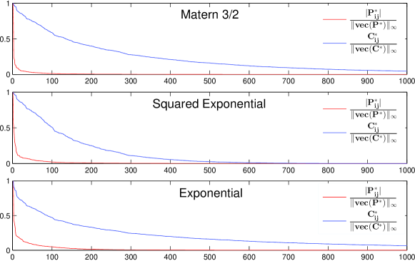
Fig. 1: Decaying behavior of elements of the Precision and Covariance matrices for GRFs. The largest 1000 off-diagonal elements of the precision and covariance matrices (scaled by their maximums) plotted in descending order. The underlying GRF was evaluated over 100 randomly selected points in $\mathcal{X}=\{\mathbf{x}\in\mathbb{R}^{2}:-50\leq\mathbf{x}\leq 50\}$ for three covariance functions with range and variance parameters equal to 10, and 1, respectively.

The method is motivated by the results in numerical linear algebra which demonstrate that if the elements of a matrix show a decay property, then the elements of its inverse also show a similar behavior – see Benzi (2016); Jaffard (1990). In particular, consider the two decay classes defined in Jaffard (1990):

Definition 1.

Given $\{\mathbf{x}_{i}\}_{i=1}^{n}\subset\mathcal{X}$ and a metric $d:\mathcal{X}\times\mathcal{X}\rightarrow\mathbb{R}_{+}$, a matrix $A\in\mathbb{R}^{n\times n}$ belongs to the class $\mathcal{E}_{\gamma}$ for some $\gamma>0$ if for all $\gamma^{\prime}<\gamma$ there exists a constant $K_{\gamma^{\prime}}$ such that $|A_{ij}|\leq K_{\gamma^{\prime}}\ \exp\big{(}-\gamma^{\prime}d(\mathbf{x}_{i},\mathbf{x}_{j})\big{)}$ for all $1\leq i,j\leq n$. Moreover, $A$ belongs to the class $\mathcal{Q}_{\gamma}$ for some $\gamma>1$ if there exists a constant $K$ such that $|A_{ij}|\leq K\ \big{(}1+d(\mathbf{x}_{i},\mathbf{x}_{j})\big{)}^{-\gamma}$ for all $1\leq i,j\leq n$.

Theorem 2.

Given $\{\mathbf{x}_{i}\}_{i=1}^{n}\subset\mathcal{X}$ and a metric $d:\mathcal{X}\times\mathcal{X}\rightarrow\mathbb{R}_{+}$, let $A\in\mathbb{R}^{n\times n}$ be an invertible matrix. If $A\in\mathcal{E}_{\gamma}$ for some $\gamma>0$, then $A^{-1}\in\mathcal{E}_{\gamma^{\prime}}$ for some $\gamma^{\prime}>0$. Moreover, if $A\in\mathcal{Q}_{\gamma}$ for some $\gamma>0$, then $A^{-1}\in\mathcal{Q}_{\gamma}$.

Proof.

See Proposition 2 and Proposition 3 in Jaffard (1990). ∎

This fast decay structure in the precision (inverse covariance) matrix of a GRF makes it a compressible signal (Candes, 2006); hence, one can argue that it can be well-approximated by a sparse matrix – compare it with the covariance matrix depicted in Figure 1. For all stationary GRFs tested, we observed that for a finite set of locations, the magnitudes of the off-diagonal elements of the precision matrix decay to 0 much faster than the elements of the covariance matrix.

Let $a^{*}$ and $b^{*}$ be given constants such that $0\leq a^{*}\leq\sigma_{\min}(P^{*})\leq\sigma_{\max}(P^{*})\leq b^{*}\leq\infty$. In the first stage of the SPS algorithm, we proposed to solve the following convex loglikelihood problem penalized with a weighted $\ell_{1}$-norm to estimate the true precision matrix corresponding to the given data locations $\mathcal{D}^{x}$:

$$\hat{P}:=\operatorname*{argmin}\{\left\langle S,P\right\rangle-\log\det(P)+\alpha\left\langle G,|P|\right\rangle:a^{*}\mathbf{I}\preceq P\preceq b^{*}\mathbf{I}\},\vspace*{-3mm}$$ (1)

where $S=\frac{1}{N}\sum_{r=1}^{N}\mathbf{y}^{(r)}{\mathbf{y}^{(r)}}^{\top}\in\mathbb{S}^{n}_{+}$ is the sample covariance matrix. The weight matrix $G\in\mathbb{S}^{n}$ is chosen as the matrix of pairwise distances:

$$G_{ij}=\|\mathbf{x}_{i}-\mathbf{x}_{j}\|,\quad\mbox{if $i\neq j$},\quad G_{ii}=\min\{\|\mathbf{x}_{i}-\mathbf{x}_{j}\|:\ j\in\mathcal{I}\setminus\{i\}\},\vspace*{-3mm}$$ (2)

for all $(i,j)\in\mathcal{I}\times\mathcal{I}$, where $\mathcal{I}=\{1,2,...,n\}$ and $|.|$ is the elementwise absolute value operator. The sparsity structure of the estimated precision matrix $\hat{P}$ encodes the conditional independence structure of a Gaussian Markov Random Field (GMRF) approximation to the GRF. Using ADMM, the Alternating Direction Method of Multipliers, see (Boyd et al., 2011), (1) can be solved efficiently. Indeed, since $-\log\det(.)$ is strongly convex and has a Lipschitz continuous gradient for $0<a^{*}\leq b^{*}<\infty$, ADMM iterate sequence converges linearly to the optimal solution with a linear rate (Deng and Yin, 2015).

In the second stage of the SPS method, we proposed to solve a least-square problem (3) to estimate the unknown parameters $\boldsymbol{\theta}^{*}$ and $\nu^{*}$:

$$(\hat{{\boldsymbol{\theta}}},\hat{\nu})=\operatorname*{argmin}_{{\boldsymbol{\theta}}\in\Theta,~{}\nu\geq 0}\|C({\boldsymbol{\theta}},\nu)-{\hat{P}}^{-1}\|_{F}^{2}.\vspace*{-3mm}$$ (3)

In Davanloo et al. (2015), we showed how to solve each optimization problem, and also established theoretical convergence rate of the SPS estimator.

SPS is therefore based on a Gaussian Markov Random Field (GMRF) approximation to the GRF. While a GMRF on a lattice can represent exactly a GRF under the conditional independence assumption, this representation of a GRF can only be an approximation in a general continuous location space. The index set is countable for the lattice data, but the index set $\mathcal{X}$ for a GRF is uncountable; hence, in general GMRF models cannot represent GRFs exactly. Lindgren et al. (2011) recently established that the Matern GRFs are Markovian; in particular, they are Markovian when the smoothing parameter $\nu$ is such that $\nu-d/2\in\mathbb{Z}_{+}$, where $d$ is the dimension of the input space – see Lindgren et al. (2011) and Fulgstad et al. (2015) for using this idea in the approximation of anisotropic and non-stationary GRFs. Rather than using a triangulation of the input space as proposed by Lindgren et al. (2011), or assuming a lattice process, the first stage of SPS lets the data determine the near-conditional independence pattern between variables through the precision matrix estimated via a weighted $\ell_{1}$-regularization. Furthermore, this first stage helps to “zoom into” the area where the true covariance parameters are located; hence, it helps not to get trapped in local optimum solutions in the second stage of the method.

3 Multivariate GRF Models

From now on, let $y(\mathbf{x})\in\mathbb{R}^{p}$ be the response vector at $\mathbf{x}\in\mathcal{X}\subseteq\mathbb{R}^{d}$ of a multivariate Gaussian Random Field (GRF) $y:\mathcal{X}\rightarrow\mathbb{R}^{p}$ with zero mean and a cross-covariance function $c(\mathbf{x},\mathbf{x}^{\prime})=\operatorname*{cov}\left(y(\mathbf{x}),y(\mathbf{x}^{\prime})\right)\in\mathbb{S}^{p}_{++}$. The cross-covariance function is a crucial object in multivariate GRF models which should converge to a symmetric and positive-definite matrix as $\|\mathbf{x}-\mathbf{x}^{\prime}\|\rightarrow 0$. Similar to the univariate case, the process is second-order stationarity if $c(.,.)$ depends on $\mathbf{x}$ and $\mathbf{x}^{\prime}$ only through $\mathbf{x}-\mathbf{x}^{\prime}$, and it is isotropic if $c(.,.)$ depends on $\mathbf{x}$ and $\mathbf{x}^{\prime}$ only through $\|\mathbf{x}-\mathbf{x}^{\prime}\|$.

The parametric structure of the cross-covariance matrix should be such that the resulting cross-covariance matrix is a positive-definite matrix. Gelfand et al. (2004) and Banerjee et al. (2014) review some methods to construct a valid cross-covariance function. In these methods, parameter estimation involves solving nonconvex optimization problems.

In this study, we assume a separable cross-covariance function belonging to a parametric family, and propose a two-stage procedure for estimating the unknown parameters. The separable model assumes that the cross-covariance function is a multiplication of a spatial correlation function and a positive-definite between-response covariance matrix (see Gelfand and Banerjee (2010); Gelfand et al. (2004) and the references therein):

$$c(\mathbf{x},\mathbf{x}^{\prime})=\rho(\mathbf{x},\mathbf{x}^{\prime})~{}\Gamma^{*}\in\mathbb{S}^{p}_{+},\vspace*{-5mm}$$ (4)

where $\rho:\mathcal{X}\times\mathcal{X}\rightarrow[0,1]$ is the spatial correlation function, and $\Gamma^{*}\in\mathbb{S}^{p}_{++}$ is the between-response covariance matrix. Furthermore, let $\mathbf{y}=[y(\mathbf{x}_{1})^{\top},...,y(\mathbf{x}_{n})^{\top}]^{\top}\in\mathbb{R}^{np}$ denote the process values in long vector form corresponding to locations in $\mathcal{D}^{x}:=\{\mathbf{x}_{i}\}_{i=1}^{n}\subset\mathcal{X}$. Given the cross-covariance function (4), and the set of locations $\mathcal{D}^{x}$, $\mathbf{y}$ follows a multivariate Gaussian distribution with zero mean and covariance matrix equal to

$$C^{*}=R^{*}\otimes\Gamma^{*},\vspace*{-3mm}$$ (5)

where $R^{*}\in\mathbb{S}^{n}_{++}$ is the spatial correlation matrix such that $R^{*}_{ij}=\rho(\mathbf{x}_{i},\mathbf{x}_{j})$ for $i,j\in\mathcal{I}:=\{1,\ldots,n\}$, and $\otimes$ denotes the Kronecker product. Hence,

$$\mathbf{y}\sim\mathcal{N}(\mathbf{0},C^{*}).\vspace*{-5mm}$$ (6)

Let $\mathcal{D}=\{(\mathbf{x}_{i},y_{i}^{(r)}):\ i\in\mathcal{I},\ r=1,...,N\}$ be the training data set that contains $N$ realizations of the process over $n$ distinct locations $\mathcal{D}^{x}\subset\mathcal{X}$, i.e., for each $r\in\{1,\ldots,N\}$, $\mathbf{y}^{(r)}=[y_{i}^{(r)}]_{i\in\mathcal{I}}\in\mathbb{R}^{np}$ is an independent realization of $\mathbf{y}=[y(\mathbf{x}_{i})]_{i\in\mathcal{I}}$. Hence, $\{\mathbf{y}^{(r)}\}_{r=1}^{N}$ are i.i.d. according to (6).

As in the univariate case, suppose the correlation function belongs to a parametric family $\{\rho(\mathbf{x},\mathbf{x}^{\prime};\boldsymbol{\theta}):\ \boldsymbol{\theta}\in\Theta\}$, where $\Theta$ is a closed convex set containing the true parameter vector, ${\boldsymbol{\theta}}^{*}$, of the correlation function $\rho$. Given $\mathcal{D}^{x}=\{\mathbf{x}_{i}\}_{i\in\mathcal{I}}$, define $R^{*}:=R({\boldsymbol{\theta}}^{*})$, where $R({\boldsymbol{\theta}})\in\mathbb{S}^{n}_{++}$ is such that

$$R({\boldsymbol{\theta}})=[r_{ij}({\boldsymbol{\theta}})]_{i,j\in\mathcal{I}},\quad r_{ij}({\boldsymbol{\theta}})=\rho(\mathbf{x}_{i},\mathbf{x}_{j};{\boldsymbol{\theta}})\quad\forall i,j\in\mathcal{I}.\vspace*{-3mm}$$ (7)

Consider a GRF model with all its parameters known, the best linear unbiased prediction at a new location $\mathbf{x}_{0}$ is given by the mean of the conditional distribution
$p(\mathbf{y}(\mathbf{x}_{0})|\{\mathbf{y}^{(r)}\}_{r=1}^{N},\mathcal{D}^{x})$ which is

$${\hat{\mathbf{y}}(\mathbf{x}_{0})=\large(\mathbf{r}(\mathbf{x}_{0};{\boldsymbol{\theta}}^{*})^{\top}\otimes\Gamma^{*}\large)\large(R({\boldsymbol{\theta}}^{*})\otimes\Gamma^{*}\large)^{-1}\sum_{r=1}^{N}\mathbf{y}^{(r)}/N,}\vspace*{-5mm}$$ (8)

where $\mathbf{r}(\mathbf{x}_{0};{\boldsymbol{\theta}}^{*})\in\mathbb{R}^{n}$ contains the spatial correlation between the new point $\mathbf{x}_{0}$ and $n$ observed data points – see (Santner et al., 2003). It is important to note that the prediction equation is a continuous function of the parameters ${\boldsymbol{\theta}}^{*}$ and $\Gamma^{*}$; hence, biased estimation of the parameters will translate to poor prediction performance. Finally, the prediction formula (8) shows the importance of considering the between-response covariance matrix $\Gamma^{*}$ rather than using $p$ independent univariate GRFs for prediction. Indeed, predicting each response independently of the others will result in suboptimal predictions.

The sample covariance matrix $S\in\mathbb{S}^{np}_{+}$ is calculated as $S=\frac{1}{N}\sum_{r=1}^{N}\mathbf{y}^{(r)}{\mathbf{y}^{(r)}}^{\top}$. Furthermore, let $G\in\mathbb{S}^{n}$ be such that $G_{ij}>0$ for all $i,j\in\mathcal{I}$; in particular, we fix $G$ as in (2) based on inter-distances. Let $P^{*}=(C^{*})^{-1}$ be the true precision matrix corresponding to locations in $\mathcal{D}^{x}$, and let $a^{*}$ and $b^{*}$ be some given constants such that $0\leq a^{*}\leq\sigma_{\min}(P^{*})\leq\sigma_{\max}(P^{*})\leq b^{*}\leq\infty$. To estimate $P^{*}$, we propose to solve the following convex program:

$$\hat{P}=\operatorname*{argmin}_{a^{*}I\preceq P\preceq b^{*}I}\left\langle S,P\right\rangle-\log\det(P)+\alpha\left\langle G\otimes(\mathbf{1}_{p}\mathbf{1}_{p}^{\top}),|P|\right\rangle,\vspace*{-3mm}$$ (9)

where $|.|$ is the element-wise absolute value operator, and $\mathbf{1}_{p}\in\mathbb{R}^{p}$ denotes the vector of all ones. This objective penalizes the elements of the precision matrix with weights proportional to the distance between their locations. Problem (9) can be solved efficiently using the ADMM implementation proposed in Davanloo et al. (2015). Indeed, for $0<a^{*}\leq b^{*}<\infty$, the function $-\log\det(.)$ is strongly convex and has a Lipschitz continuous gradient; therefore, the ADMM sequence converges linearly to the optimal solution – see Deng and Yin (2015).

Let $\hat{C}:=\hat{P}^{-1}$, and for all $(i,j)\in\mathcal{I}\times\mathcal{I}$ define block matrices $S^{ij}\in\mathbb{S}^{p}$, $\hat{C}^{ij}\in\mathbb{S}^{p}$ and $\Sigma^{ij}\in\mathbb{S}^{p}$ such that $S=[S^{ij}]$, $\hat{C}=[\hat{C}^{ij}]$ and $C^{*}=[\Sigma^{ij}]$, i.e., $S^{ij}\in\mathbb{S}^{p}$, $\hat{C}^{ij}\in\mathbb{S}^{p}$ and $\Sigma^{ij}\in\mathbb{S}^{p}$ are the sample, estimated and true covariance matrices between the locations $\mathbf{x}_{i}$ and $\mathbf{x}_{j}$. The following establishes a probability bound for the estimation error $\hat{P}-P^{*}$.

Theorem 3.

Let $\{\mathbf{y}^{(r)}\}_{r=1}^{N}\subset\mathbb{R}^{nq}$ be independent realizations of a GRF with zero-mean and stationary covariance function $c(\mathbf{x},\mathbf{x}^{\prime};\boldsymbol{\theta}^{*})$ observed over $n$ distinct locations $\{\mathbf{x}_{i}\}_{i\in\mathcal{I}}$ with $\mathcal{I}:=\{1,...,n\}$; furthermore, let $C^{*}=R({\boldsymbol{\theta}}^{*})\otimes\Gamma^{*}$ be the true covariance matrix, and $P^{*}:={C^{*}}^{-1}$ be the corresponding true precision matrix, where $R({\boldsymbol{\theta}})$ is defined in (7). Finally, let $\hat{P}$ be the GSPS estimator computed as in (9) for some $G\in\mathbb{S}^{n}$ such that $G_{ij}\geq 0$ for all $(i,j)\in\mathcal{I}\times\mathcal{I}$. Then for any given $M>0$, $N\geq N_{0}:=\left\lceil 2\big{[}(M+2)\ln(np)+\ln 4\big{]}\right\rceil$, and $b^{*}\geq\sigma_{\max}(P^{*})$,

$$\mbox{Pr}\left(\|\hat{P}-P^{*}\|_{F}\leq 2{b^{*}}^{2}p(n+\|G\|_{F})\alpha\right)\geq 1-(np)^{-M},\vspace*{-3mm}$$ (10)

for all $\alpha$ such that $40\max\limits_{i=1,...,p}(\Gamma_{ii}^{*})\sqrt{\frac{N_{0}}{N}}\leq\alpha\leq 40\max\limits_{i=1,...,p}(\Gamma_{ii}^{*})$.

Proof.

See the appendix. ∎

Given that $C^{*}=R^{*}\otimes\Gamma^{*}$, and the diagonal elements of the spatial correlation matrix $R^{*}$ are equal to one, we have $\Sigma^{ii}=\Gamma^{*}$. Therefore, we propose to estimate the between-response covariance matrix $\Gamma^{*}$ by taking the average of the $p\times p$ matrices along the diagonal of $\hat{C}$, i.e.,

$$\hat{\Gamma}:=\frac{1}{n}\sum_{i=1}^{n}\hat{C}^{ii}\in\mathbb{S}^{n}_{++}.\vspace*{-4mm}$$ (11)

Note that (9) implies that $\hat{P}\in\mathbb{S}^{np}_{++}$; hence, $\hat{C}\in\mathbb{S}^{np}_{++}$ as well. Therefore, all its block-diagonal elements are positive definite, i.e., $\hat{\Sigma}^{ii}\in\mathbb{S}^{n}_{++}$ for $i=1,...,n$. Since $\hat{\Gamma}$ is a convex combination of $\hat{\Sigma}^{ii}\in\mathbb{S}^{n}_{+},\ i=1,...,n$ and the cone of positive definite matrices is a convex set, we also have $\hat{\Gamma}\in\mathbb{S}^{n}_{++}$. A probability bound in the estimation error of the covariance matrices is shown in the following theorem.

Theorem 4.

Given $M>0$, $N\geq N_{0}:=\left\lceil 2\big{[}(M+2)\ln(np)+\ln 4\big{]}\right\rceil$, and $a^{*}$, $b^{*}$ such that $0<a^{*}\leq\sigma_{\min}(P^{*})\leq\sigma_{\max}(P^{*})\leq b^{*}<\infty$, let $\hat{P}$ be the SPS estimator as in (9). Then $\hat{\Gamma}$, defined in (11), and $\hat{C}=\hat{P}^{-1}$ satisfy

$$\mbox{Pr}\left(\max\{\|\hat{C}-C^{*}\|_{2},~{}\|\hat{\Gamma}-\Gamma^{*}\|_{2}\}\leq 2\left(\frac{b^{*}}{a^{*}}\right)^{2}p(n+\|G\|_{F})\alpha\right)\geq 1-(np)^{-M},\vspace*{-3mm}$$

for all $\alpha$ such that $40\max\limits_{i=1,...,p}(\Gamma_{ii}^{*})\sqrt{\frac{N_{0}}{N}}\leq\alpha\leq 40\max\limits_{i=1,...,p}(\Gamma_{ii}^{*})$.

Proof.

From (10), we have

$$\|\hat{C}-C^{*}\|_{2}\leq\frac{1}{{a^{*}}^{2}}\|\hat{P}-P^{*}\|_{2}\leq\frac{1}{{a^{*}}^{2}}\|\hat{P}-P^{*}\|_{F}\leq 2\left(\frac{b^{*}}{a^{*}}\right)^{2}p(n+\|G\|_{F})\alpha,\vspace*{-3mm}$$

where the first inequality follows from the Lipschitz continuity of $P\mapsto P^{-1}$ on the domain $P\succeq a^{*}\mathbf{I}$ with respect to the spectral norm $\|.\|_{2}$. Hence, given that $\Gamma^{*}=\Sigma^{ii}$ for all $i\in\mathcal{I}$, we have $\|\hat{C}^{ii}-\Gamma^{*}\|_{2}\leq 2\left(\frac{b^{*}}{a^{*}}\right)^{2}p(n+\|G\|_{F})\alpha$ for all $i\in\mathcal{I}$. Therefore, from convexity of $X\mapsto\|X-\Gamma^{*}\|_{2}$, it follows that

$$\|\hat{\Gamma}-\Gamma^{*}\|_{2}\leq\sum_{i\in\mathcal{I}}\frac{1}{n}\|\hat{C}^{ii}-\Gamma^{*}\|_{2}\leq 2\left(\frac{b^{*}}{a^{*}}\right)^{2}p(n+\|G\|_{F})\alpha.\vspace*{-1.2cm}$$

∎

Remark. For Theorems 2 and 3 to hold, $\alpha$ should belong to the interval $40\max\limits_{i=1,...,p}(\Gamma_{ii}^{*})\sqrt{\frac{N_{0}}{N}}\leq\alpha\leq 40\max\limits_{i=1,...,p}(\Gamma_{ii}^{*})$; for $N\geq N_{0}$ this interval is non-empty. The trade-off here is such that smaller $\alpha$ makes the estimation error bounds inside the probabilities tighter – hence, desirable; however, at the same time, smaller $\alpha$ makes the estimated precision matrix less sparse which would require more memory to store a denser estimated precision matrix. Although the upper-bound on $\alpha$ is fixed, one can play with the lower bound; in particular, one can make it smaller by requiring more realizations $N$.

Given $\mathcal{D}^{x}=\{\mathbf{x}_{i}\}_{i\in\mathcal{I}}\subset\mathcal{X}$, define $R:\mathbb{R}^{q}\rightarrow\mathbb{S}^{n}$ over $\Theta\subset\mathbb{R}^{q}$ as in (7), i.e., $R({\boldsymbol{\theta}})=[r_{ij}({\boldsymbol{\theta}})]_{i,j\in\mathcal{I}}\in\mathbb{S}^{n}$ and $r_{ij}({\boldsymbol{\theta}})=\rho(\mathbf{x}_{i},\mathbf{x}_{j};{\boldsymbol{\theta}})$ for all $(i,j)\in\mathcal{I}\times\mathcal{I}$. To estimate the true parameter vector of the spatial correlation function, ${\boldsymbol{\theta}}^{*}$, we propose to solve

$$\hat{{\boldsymbol{\theta}}}\in\operatorname*{argmin}_{{\boldsymbol{\theta}}\in\Theta}\frac{1}{2}\sum_{i,j\in\mathcal{I}}\|r_{ij}({\boldsymbol{\theta}})\hat{\Gamma}-\hat{C}^{ij}\|_{F}^{2}.\vspace*{-5mm}$$ (12)

The objective function of (12) can be written in a more compact form as the parametric function below, with parameters $\Gamma\in\mathbb{S}^{p}$ and $C\in\mathbb{S}^{np}$:

$$f({\boldsymbol{\theta}};\Gamma,C):=\frac{1}{2}\|R({\boldsymbol{\theta}})\otimes\Gamma-C\|_{F}^{2}.\vspace*{-3mm}$$ (13)

Let ${\boldsymbol{\theta}}=[\theta_{1},\ldots,\theta_{q}]^{\top}$, and $R_{k}^{\prime}:\mathbb{R}^{q}\rightarrow\mathbb{S}^{n}$ such that $R_{k}^{\prime}({\boldsymbol{\theta}})=[\frac{\partial}{\partial\theta_{k}}r_{ij}({\boldsymbol{\theta}})]_{i,j\in\mathcal{I}}$ for $k=1,\ldots,q$. Similarly, $R_{k\ell}^{{}^{\prime\prime}}:\mathbb{R}^{q}\rightarrow\mathbb{S}^{n}$ such that $R_{k\ell}^{{}^{\prime\prime}}({\boldsymbol{\theta}})=[\frac{\partial^{2}}{\partial\theta_{k}\partial\theta_{\ell}}r_{ij}({\boldsymbol{\theta}})]_{i,j\in\mathcal{I}}$ for $1\leq k,\ell\leq q$. Let $Z({\boldsymbol{\theta}};\Gamma,C):=R({\boldsymbol{\theta}})\otimes\Gamma-C$; hence, $f({\boldsymbol{\theta}};\Gamma,C)=\|Z({\boldsymbol{\theta}};\Gamma,C)\|_{F}^{2}/2$; and define $Z_{k}^{\prime}({\boldsymbol{\theta}};\Gamma):=R_{k}^{\prime}({\boldsymbol{\theta}})\otimes\Gamma$ for $k=1,\ldots,q$.

Lemma 5.

Suppose $\rho(\mathbf{x},\mathbf{x}^{\prime};{\boldsymbol{\theta}})$ is twice continuously differentiable in ${\boldsymbol{\theta}}$ over $\Theta$ for all $\mathbf{x},\mathbf{x}^{\prime}\in\mathcal{X}$, then there exists $\gamma^{*}>0$ such that $\nabla^{2}_{\boldsymbol{\theta}}f({\boldsymbol{\theta}}^{*};\Gamma^{*},C^{*})\succeq\gamma^{*}\mathbf{I}$ if and only if $\{\mathop{\bf vec}(R^{\prime}_{k}({\boldsymbol{\theta}}^{*}))\}_{k=1}^{q}\subset\mathbb{R}^{n^{2}}$ are linearly independent.

Proof.

Clearly, $\nabla_{\boldsymbol{\theta}}f({\boldsymbol{\theta}};\Gamma,C)=\left[\left\langle Z_{1}^{\prime}({\boldsymbol{\theta}};\Gamma),Z({\boldsymbol{\theta}};\Gamma,C)\right\rangle,\ldots,\left\langle Z_{q}^{\prime}({\boldsymbol{\theta}};\Gamma),Z({\boldsymbol{\theta}};\Gamma,C)\right\rangle\right]^{\top}$.
Hence, it can be shown that for $1\leq k\leq q$

$$\frac{\partial}{\partial\theta_{k}}f({\boldsymbol{\theta}};\Gamma,C)=\|\Gamma\|_{F}^{2}\left\langle R_{k}^{\prime}({\boldsymbol{\theta}}),R({\boldsymbol{\theta}})\right\rangle-\left\langle C,R_{k}^{\prime}({\boldsymbol{\theta}})\otimes\Gamma\right\rangle,\vspace*{-3mm}$$ (14)

and from the product rule for derivatives, it follows that for $1\leq k,\ell\leq q$

$$\frac{\partial^{2}}{\partial\theta_{k}\partial\theta_{\ell}}f({\boldsymbol{\theta}};\Gamma,C)=\|\Gamma\|_{F}^{2}\left\langle R_{k}^{\prime}({\boldsymbol{\theta}}),R_{\ell}^{\prime}({\boldsymbol{\theta}})\right\rangle+\left\langle R_{k\ell}^{{}^{\prime\prime}}({\boldsymbol{\theta}})\otimes\Gamma,R({\boldsymbol{\theta}})\otimes\Gamma-C\right\rangle.\vspace*{-8mm}$$ (15)

Thus, since $C^{*}=r({\boldsymbol{\theta}}^{*})\otimes\Gamma^{*}$, we have

$$\frac{\partial^{2}}{\partial\theta_{k}\partial\theta_{\ell}}f({\boldsymbol{\theta}};\Gamma^{*},C^{*})=\|\Gamma^{*}\|_{F}^{2}\left\langle R_{k}^{\prime}({\boldsymbol{\theta}}^{*}),R_{\ell}^{\prime}({\boldsymbol{\theta}}^{*})\right\rangle.\vspace*{-3mm}$$

Therefore, $\nabla^{2}_{\boldsymbol{\theta}}f({\boldsymbol{\theta}}^{*};\Gamma^{*},C^{*})=\|\Gamma^{*}\|_{F}^{2}~{}J({\boldsymbol{\theta}}^{*})^{\top}J({\boldsymbol{\theta}}^{*})$, where $J({\boldsymbol{\theta}})\in\mathbb{R}^{n^{2}\times q}$ such that $J({\boldsymbol{\theta}}):=[\mathop{\bf vec}(R_{1}^{\prime}({\boldsymbol{\theta}}))\ldots\mathop{\bf vec}(R_{q}^{\prime}({\boldsymbol{\theta}}))]$. Hence, there exists $\gamma^{*}>0$ such that $\nabla^{2}_{\boldsymbol{\theta}}f({\boldsymbol{\theta}}^{*};\Gamma^{*},C^{*})\succeq\gamma^{*}I$ when $\{\mathop{\bf vec}(R_{k}^{\prime}({\boldsymbol{\theta}}^{*}))\}_{k=1}^{q}\subset\mathbb{R}^{n^{2}}$ are linearly independent. ∎

Remark. We comment on the linear independence condition stated in Lemma 5. For illustration purposes, consider the anisotropic exponential correlation function $\rho(\mathbf{x},\mathbf{x}^{\prime},{\boldsymbol{\theta}})=\exp\big{(}-(\mathbf{x}-\mathbf{x}^{\prime})^{\top}\mathop{\operator@font diag}\nolimits({\boldsymbol{\theta}})(\mathbf{x}-\mathbf{x}^{\prime})\big{)}$, where $q=d$, and $\Theta=\mathbb{R}^{d}_{+}$. Let $\mathcal{X}=[-\beta,\beta]^{d}$ for some $\beta>0$, and suppose $\{\mathbf{x}_{i}\}_{i\in\mathcal{I}}$ is a set of independent identically distributed uniform random samples inside $\mathcal{X}$. Then it can be easily shown that for the anisotropic exponential correlation function, the condition in Lemma 5 holds with probability 1, i.e., $\{\mathop{\bf vec}(R_{k}^{\prime}({\boldsymbol{\theta}}^{*}))\}_{k=1}^{d}$ are linearly independent w.p. 1.

The next result builds on Lemma 5, and it shows the convergence of the GSPS estimator as the number of samples per location, $N$, increases.

Theorem 6.

Suppose ${\boldsymbol{\theta}}^{*}\in\mathop{\bf int}{\boldsymbol{\Theta}}$, and $\rho(\mathbf{x},\mathbf{x}^{\prime};{\boldsymbol{\theta}})$ is twice continuously differentiable in ${\boldsymbol{\theta}}$ over $\Theta$ for all $\mathbf{x},\mathbf{x}^{\prime}\in\mathcal{X}$. Suppose $\{\mathop{\bf vec}(R^{\prime}_{k}({\boldsymbol{\theta}}^{*}))\}_{k=1}^{q}\subset\mathbb{R}^{n^{2}}$ are linearly independent. For any given $M>0$ and $N\geq N_{0}:=\left\lceil 2(M+2)\ln(np)+\ln 16\right\rceil$, let $\hat{{\boldsymbol{\theta}}}^{(N)}$ be the GSPS estimator of ${\boldsymbol{\theta}}^{*}$, i.e., $\hat{{\boldsymbol{\theta}}}=\operatorname*{argmin}_{{\boldsymbol{\theta}}\in\Theta}f({\boldsymbol{\theta}};\hat{\Gamma},\hat{C})$, and $\hat{\Gamma}$ be computed as in (11). Then for any sufficiently small $\epsilon>0$, there exists $N\geq N_{0}$ satisfying $N=\mathcal{O}(N_{0}/\epsilon^{2})$ such that setting $\alpha=40\max_{i=1,\ldots,p}(\Gamma^{*}_{ii})\sqrt{\frac{N_{0}}{N}}$ in (9) implies $\|\hat{{\boldsymbol{\theta}}}^{(N)}-{\boldsymbol{\theta}}^{*}\|\leq\epsilon$ and $\|\hat{\Gamma}-\Gamma^{*}\|=\mathcal{O}(\epsilon)$ with probability at least $1-(np)^{-M}$; moreover, the STAGE-II function $f(\cdot;\hat{\Gamma},\hat{C})$ is strongly convex around the estimator $\hat{{\boldsymbol{\theta}}}$.

Proof.

See the appendix. ∎

Remark. In Theorem 4, $\alpha$ is explicitly set equal to the lower bound, i.e.,
$\alpha=40\max\limits_{i=1,...,p}(\Gamma_{ii}^{*})\sqrt{\frac{N_{0}}{N}}=40\max\limits_{i=1,...,p}(\Gamma_{ii}^{*})\sqrt{\frac{\left\lceil 2\big{[}(M+2)\ln(np)+\ln 4\big{]}\right\rceil}{N}}$. Note that $M$ controls the probability bound; hence, the only unknown is $\max\limits_{i=1,...,p}(\Gamma_{ii}^{*})$ – we implicitly assume that this quantity can be estimated empirically or we have a prior knowledge about it. Moreover, Theorem 4 also guides us how to select $\alpha$. Indeed, both $\|\hat{{\boldsymbol{\theta}}}^{(N)}-{\boldsymbol{\theta}}^{*}\|\leq\epsilon$ and $\|\hat{\Gamma}-\Gamma^{*}\|=\mathcal{O}(\epsilon)$ whenever $N=\mathcal{O}(N_{0}/\epsilon^{2})$; therefore, this implies we should set $\alpha=\mathcal{O}(\epsilon)$. In the simulations provided in Section 4, $\alpha$ is set equal to $c\sqrt{\log(np)/N}$ where $c$ is chosen $10^{-2}$ after some preliminary cross-validation studies.

A summary of the proposed algorithm for fitting multivariate GRFs models is provided in Algorithm 1.

Algorithm 1 GSPS algorithm to fit multivariate GRFs

input: $\mathcal{D}=\{(\mathbf{x}_{i},\mathbf{y}_{i}^{(r)})\}_{i=1}^{n}\subset\mathcal{X}\times\mathbb{R}^{p},\ i\in\mathcal{I},\ r=1,...,N\}$
/* Compute the sample covariance and distance matrices*/
      $\mathbf{y}^{(r)}\leftarrow[\mathbf{y}(\mathbf{x}_{1})^{T},...,\mathbf{y}(\mathbf{x}_{n})^{T}]^{T}\in\mathbb{R}^{np},\ r=1,...,N$
      $S\leftarrow\frac{1}{N}\sum_{r=1}^{N}\mathbf{y}^{(r)}{\mathbf{y}^{(r)}}^{\top}$
      $G_{ij}\leftarrow\|\mathbf{x}_{i}-\mathbf{x}_{j}\|_{2},\quad\mbox{if}\ i\neq j$, $G_{ii}\leftarrow\min\{\|\mathbf{x}_{i}-\mathbf{x}_{j}\|_{2}:\ j\in\mathcal{I}\setminus\{i\}$
/* Compute the precision matrix and its inverse */
      $\hat{P}\leftarrow\operatorname*{argmin}\{\left\langle S,P\right\rangle-\log\det(P)+\alpha\left\langle G\otimes(\mathbf{1}_{q}\mathbf{1}_{q}^{T}),|P|\right\rangle:\ a^{*}\mathbf{I}\preceq P\preceq b^{*}\mathbf{I}\}$
     $\hat{C}\leftarrow\hat{P}^{-1}$
/* Compute the between response covariance matrix */
      $\hat{\Gamma}\leftarrow\frac{1}{n}\sum_{i\in\mathcal{I}}\hat{C}^{ii}$
/* Compute the spatial correlation parameter vector*/
      $\hat{{\boldsymbol{\theta}}}\leftarrow\operatorname*{argmin}_{{\boldsymbol{\theta}}\in\Theta}\frac{1}{2}\sum_{i,j\in\mathcal{I}}\|\rho_{ij}({\boldsymbol{\theta}})~{}\hat{\Gamma}-\hat{C}^{ij}\|_{F}^{2}$
return: $\hat{\Gamma}$ and $\hat{{\boldsymbol{\theta}}}$

3.1. Connection to SPS. The main difference between the SPS method and GSPS is how $\hat{\Gamma}$, the estimator for $\Gamma^{*}$, is computed (when $p=1$, $\Gamma^{*}\in\mathbb{R}_{++}$ corresponds to the variance parameter $\nu^{*}>0$ in SPS), and this difference in the way $\Gamma^{*}$ is estimated has significant implications on: a) the numerical stability of solving STAGE-II problem, and b) the proof technique to show consistency of the hyperparameter estimate as the number of process realization, $N$, increases.

In the derivation of SPS, we considered the estimate $\hat{\nu}({\boldsymbol{\theta}})$ as an optimal response to the spatial correlation parameter ${\boldsymbol{\theta}}$, and show that $\hat{\nu}({\boldsymbol{\theta}})$ can be written in a closed form. In the second stage problem of SPS, given in (3), we solve a least squares problem over ${\boldsymbol{\theta}}$, i.e.,

$$\hat{{\boldsymbol{\theta}}}=\operatorname*{argmin}_{{\boldsymbol{\theta}}\in\mathbb{R}_{+}^{d}}\tfrac{1}{2}\sum_{i,j}(\hat{\nu}({\boldsymbol{\theta}})\rho(\mathbf{x}_{i},\mathbf{x}_{j},{\boldsymbol{\theta}})-\hat{C}_{ij})^{2}.\vspace*{-7mm}$$

Once $\hat{{\boldsymbol{\theta}}}$ is computed, we estimate $\nu^{*}$ using the best response function: $\hat{\nu}=\hat{\nu}(\hat{{\boldsymbol{\theta}}})$. The problem we observed with this approach in Davanloo et al. (2015) when applied to hyper-parameter estimation of a multivariate GRF is that the second stage problem becomes challenging due to its strong nonconvexity, which is significantly aggravated relative to the univariate case due to the multiplicative structure of $\hat{\Gamma}({\boldsymbol{\theta}})\rho(\mathbf{x}_{i},\mathbf{x}_{j},{\boldsymbol{\theta}})$ (when there is a single response, $p=1$, this was not a problem for SPS). However, when $p>1$, this same structure causes numerical problems in the STAGE-II problem as one would need to solve

$$\min_{{\boldsymbol{\theta}}\in\mathbb{R}_{+}^{d}}\tfrac{1}{2}\|R({\boldsymbol{\theta}})\otimes\hat{\Gamma}({\boldsymbol{\theta}})-\hat{C}\|_{F}^{2}.\vspace*{-5mm}$$ (16)

Compared to the above problem, the STAGE-II problem we proposed in (12) for GSPS, i.e., $\min_{{\boldsymbol{\theta}}\in\mathbb{R}_{+}^{d}}\tfrac{1}{2}\|R({\boldsymbol{\theta}})\otimes\hat{\Gamma}-\hat{C}\|_{F}^{2}$, behaves much better (although it is also non-convex in general), where $\hat{\Gamma}=\tfrac{1}{n}\sum_{i=1}^{n}\hat{C}_{ii}$ – note that Theorem 6 shows that the STAGE-II objective of GSPS is strongly convex around a neighborhood of the estimator. In all our numerical tests, standard nonlinear optimization techniques were able to compute a point close to the global minimizer very efficiently; however, this was not the case for the problem in (16) when $p>1$ – the same nonlinear optimization solvers we used for GSPS get stuck at a local minimizer far away from the global minimum. This is why we propose GSPS using (12) in this paper. Moreover, this new step of estimating $\hat{\Gamma}=\tfrac{1}{n}\sum_{i=1}^{n}\hat{C}_{ii}$ also helps us to give a much simpler proof for Theorem 4.

We now comment on using GSPS to fit a multivariate GRF as opposed to using SPS to fit $p$ independent univariate GRFs to $p$ responses. As mentioned earlier, the latter can only be suboptimal in the presence of cross-covariances between the responses. Furthermore, fitting a multivariate anisotropic GRF requires estimating $p(p+1)/2$ parameters for the between-response covariance matrix $\Gamma^{*}\in\mathbb{S}^{p}_{++}$ and $d$ parameters for the anisotropic spatial correlation function ${\boldsymbol{\theta}}\in\Theta\subseteq\mathbb{R}^{d}_{++}$. On the other hand, fitting $p$ independent univariate anisotropic GRF requires estimating $p(d+1)$ parameters, i.e., for each univariate GRF one needs to estimate $d$ spatial correlation parameters and $1$ variance parameter. Therefore, if $d>\frac{p}{2}$, then fitting $p$ univariate GRF requires estimating more hyperparameters. Indeed, for some machine learning problems we have $d\gg p$, e.g., the classification problem for text categorization (Joachims, 1998) with $p>1$ related classes, and for these type of problems $d$ could be $\approx 10000$ and estimating $pd$ hyper-parameters will lead to overfitting; hence, its prediction performance on test data will be worse compared to the prediction performance for multivariate GRF using (8) with ${\boldsymbol{\theta}}^{*}$ and $\Gamma^{*}$ replaced by $\hat{{\boldsymbol{\theta}}}$ and $\hat{\Gamma}$ which are computed as in (12) and (11), respectively – see Theorem 6 for bounds on hyper-parameter approximation quality. In Sections 4.2 and 4.3, the numerical tests conducted on simulated and real-data also show that the proposed GSPS method performs significantly better than modeling each response independently.

3.2. Computational Complexity. The computational bottleneck of GSPS method is the singular value decompositions (SVD) that arises when solving the STAGE-I problem using the ADMM algorithm. The per-iteration complexity is $\mathcal{O}((np)^{3})$. However, we should note that the STAGE-I problem is strongly convex; and ADMM has a linear rate (Deng and Yin, 2015). Therefore, an $\epsilon$-optimal solution can be computed within $\mathcal{O}(\log(1/\epsilon))$ iterations of ADMM. Thus, the overall complexity of solving STAGE-I is $\mathcal{O}((np)^{3}~{}\log(1/\epsilon))$. Note that likelihood approximation methods do not have such iteration complexity results due to the non-convexity of the approximate likelihood problem being solved, even though they have cheaper per-iteration-complexity. In case of an isotropic process, the STAGE-II problem in (12) is one dimensional and it can simply be solved by using bisection. If the process is anisotropic, then (12) is non-convex in general. That said, this problem is low dimensional due to $d\ll n$; hence, standard nonlinear optimization techniques can compute a local minimizer very efficiently – note that we also show that STAGE-II objective is strongly convex around a neighborhood of the estimator. In all our numerical tests, STAGE-II problem is solved in much shorter time compared to STAGE-I problem; hence, it does not affect the overall complexity significantly. In our code, we use golden-section search for isotropic processes, and Knitro’s nonconvex solver to solve (12) for general anisotropic processes.

To eliminate $\mathcal{O}((np)^{3})$ complexity due to an SVD computation per ADMM iteration and due to computing $\hat{C}$, we used a segmentation scheme. We partition the data to $K$ segments, each one composed of $\approx n/K$ points chosen uniformly at random among $n$ locations, and assuming conditional independence between blocks. In (Davanloo et al., 2015), we discussed two blocking/segmentation schemes: Spatial Segmentation (SS) and Random Selection (RS). Solving the STAGE-I problem with blocking schemes assumes a conditional independence assumption between blocks. In SS scheme such conditional independence assumption is potentially violated for points along the common boundary between two blocks. The RS scheme, however, works numerically better for “big-n” scenarios. We believe that with RS scheme the infill asymptotics make the blocks conditionally independent to a reasonable degree. Using such blocking schemes, the bottleneck complexity reduces to $\mathcal{O}((np/K)^{3})$ by solving STAGE-I problem for each block; hence, solving STAGE-I and computing $\hat{C}$, which we assume to be block diagonal, requires a total complexity of $\mathcal{O}(\log(1/\epsilon)~{}(np)^{3}/K^{2})$ and this bottleneck complexity can be controlled by properly choosing $K$.

4. Numerical results

In this section, comprehensive simulation analyses are reported for the study of the performance of the proposed method. $N$ realizations of a zero-mean $p$-variate GRF with anisotropic spatial correlation function are simulated in a square domain $\mathcal{X}=[0,10]^{d}$ over $n$ distinct points. The separable covariance function is the product of an anisotropic exponential spatial correlation function $\rho(\mathbf{x},\mathbf{x}^{\prime},{\boldsymbol{\theta}}^{*})=\exp\big{(}-(\mathbf{x}-\mathbf{x}^{\prime})^{\top}\mathop{\operator@font diag}\nolimits({\boldsymbol{\theta}}^{*})(\mathbf{x}-\mathbf{x}^{\prime})\big{)}$ and a $p$-variate between-response covariance matrix $\Gamma^{*}\in\mathbb{S}^{p}_{++}$. The correlation function parameter vector ${\boldsymbol{\theta}}^{*}_{\ell}$ is sampled uniformly from the surface of a hyper-sphere in $\mathbb{R}^{d}$ in the positive orthant for each replication $\ell\in\{1,...,L\}$. The between-response covariance matrix is $\Gamma^{*}_{\ell}=A^{\top}A$ for $A\in\mathbb{R}^{w\times p}$ such that $w>p$, where the elements of $A$ are sampled independently from $\mathcal{N}(0,1)$ per replication. To solve the STAGE-I problem, the sparsity parameter $\alpha$ in (1) is set equal to $c\sqrt{\log(np)/N}$ for some constant $c$. After some preliminary cross-validation studies, we set $c$ equal to $10^{-2}$. In our code, we use golden-section search for isotropic processes which requires a univariate optimization in STAGE-II, and use Knitro’s nonconvex solver to solve (12) for general anisotropic processes.

4.1. Parameter estimate consistency

We first compare the quality of GSPS parameter estimate with the Maximum Likelihood Estimate (MLE). For 10 different replicates, we simulated $N$ independent realizations of GRF described above under different scenarios, and the mean of $\{\|\hat{{\boldsymbol{\theta}}}_{\ell}-{\boldsymbol{\theta}}^{*}\|\}_{\ell=1}^{10}$ and $\{\|\hat{\Gamma}_{\ell}-\Gamma^{*}\|_{F}\}_{\ell=1}^{10}$ are reported.

To deal with the nonconcavity of the likelihood, the MLEs are calculated from 10 random initial solutions and the best final solutions are reported. To solve problem in (9) for the scenarios with $np>2000$, we used the Random Selection (RS) blocking scheme as described in Davanloo et al. (2015). Tables 1 and 2 show the results for $p$-variate GRF models with $p=2$ and $p=5$, respectively.

			N=1		N=10		N=40
d	n	Method	$\|\hat{{\boldsymbol{\theta}}}_{l}-{\boldsymbol{\theta}}^{*}\|_{2}$	$\|\hat{\Gamma}_{\ell}-\Gamma^{*}\|_{F}$	$\|\hat{{\boldsymbol{\theta}}}_{l}-{\boldsymbol{\theta}}^{*}\|_{2}$	$\|\hat{\Gamma}_{\ell}-\Gamma^{*}\|_{F}$	$\|\hat{{\boldsymbol{\theta}}}_{l}-{\boldsymbol{\theta}}^{*}\|_{2}$	$\|\hat{\Gamma}_{\ell}-\Gamma^{*}\|_{F}$	Time (sec)
2	100	GSPS	0.43	0.89	0.34	0.66	0.21	0.53	14.9
		MLE	0.38	0.78	0.36	0.70	0.26	0.61	21.3
	500	GSPS	0.39	0.81	0.29	0.60	0.13	0.43	312.3
		MLE	0.37	0.83	0.32	0.62	0.19	0.50	496.1
	1000	GSPS	0.33	0.73	0.23	0.57	0.08	0.34	2342.5
		MLE	0.32	0.74	0.28	0.58	0.11	0.40	3216.5
5	100	GSPS	0.49	0.96	0.38	0.71	0.26	0.56	18.9
		MLE	0.46	0.93	0.42	0.71	0.36	0.61	36.5
	500	GSPS	0.44	0.88	0.33	0.69	0.29	0.53	527.4
		MLE	0.46	0.89	0.38	0.67	0.34	0.59	1023.4
	1000	GSPS	0.40	0.81	0.30	0.62	0.29	0.50	2987.3
		MLE	0.43	0.92	0.35	0.66	0.34	0.56	6120.8
10	100	GSPS	0.55	1.05	0.39	0.82	0.35	0.58	29.1
		MLE	0.57	1.02	0.56	0.89	0.53	0.69	75.2
	500	GSPS	0.47	0.99	0.35	0.73	0.31	0.49	613.8
		MLE	0.54	1.00	0.53	0.81	0.50	0.58	4125.6
	1000	GSPS	0.41	0.89	0.31	0.71	0.29	0.43	4920.5
		MLE	0.51	0.97	0.49	0.76	0.47	0.50	7543.3

Table 1: Comparison of GSPS vs. MLE for p=2 response variables

			N=1		N=10		N=40
d	n	Method	$\|\hat{{\boldsymbol{\theta}}}_{l}-{\boldsymbol{\theta}}^{*}\|_{2}$	$\|\hat{\Gamma}_{\ell}-\Gamma^{*}\|_{F}$	$\|\hat{{\boldsymbol{\theta}}}_{l}-{\boldsymbol{\theta}}^{*}\|_{2}$	$\|\hat{\Gamma}_{\ell}-\Gamma^{*}\|_{F}$	$\|\hat{{\boldsymbol{\theta}}}_{l}-{\boldsymbol{\theta}}^{*}\|_{2}$	$\|\hat{\Gamma}_{\ell}-\Gamma^{*}\|_{F}$	Time (sec)
2	100	GSPS	0.66	1.43	0.38	0.91	0.30	0.76	17.2
		MLE	0.62	1.40	0.57	1.30	0.41	1.28	26.3
	500	GSPS	0.58	1.35	0.35	0.87	0.27	0.73	363.4
		MLE	0.57	1.32	0.51	1.24	0.39	1.15	512.5
	1000	GSPS	0.49	1.24	0.31	0.82	0.24	0.70	2835.4
		MLE	0.49	1.22	0.42	1.19	0.33	1.10	3913.7
5	100	GSPS	0.73	1.49	0.50	0.92	0.39	0.79	25.6
		MLE	0.71	1.47	0.62	1.36	0.49	1.35	53.1
	500	GSPS	0.60	1.41	0.44	1.00	0.36	0.75	665.6
		MLE	0.64	1.43	0.54	1.26	0.44	1.24	1424.3
	1000	GSPS	0.54	1.32	0.39	1.06	0.31	0.74	3783.6
		MLE	0.63	1.36	0.47	1.20	0.38	1.17	7346.7
10	100	GSPS	0.77	1.57	0.59	0.98	0.52	0.85	45.3
		MLE	0.79	1.60	0.67	1.39	0.61	1.43	87.2
	500	GSPS	0.65	1.47	0.54	1.03	0.46	0.81	717.6
		MLE	0.74	1.56	0.60	1.31	0.52	1.37	4994.3
	1000	GSPS	0.59	1.39	0.49	1.08	0.42	0.75	6001.3
		MLE	0.66	1.48	0.53	1.27	0.45	1.29	8223.1

Table 2: Comparison of GSPS vs. MLE for p=5 response variables

For fixed $n$, the parameter estimation error increases with the dimension of the input space $d$, which is reasonable due to higher number of parameters in the anisotropic correlation function. Furthermore, the errors increase with $p$, the number of responses. As expected, increasing the point density $n$ helps in improving the estimation of the parameters, i.e., reducing the errors, a result in accordance to the expected effect of infill asymptotics.

Overall, the GSPS method results in better parameter estimates compared to MLE with relative performance improvements becoming more obvious as $p$ and $d$ increase. Furthermore, as the number of realizations $N$ increases GSPS performs consistently better than MLE. Note that the robust performance of the proposed method is theoretically guaranteed for $N\geq N_{0}$ from Theorem 6.

4.2. Prediction consistency

To evaluate prediction performance, we compared the GSPS method against using multiple univariate SPS (mSPS) fits and against the Convolved Multiple output Gaussian Process (CMGP) method by Alvarez and Lawrence (2011). Given the size of the training data $n$, none of the approximations in (Alvarez and Lawrence, 2011) with induced points were used, this corresponds to what Alvarez and Lawrence refer as the CMGP method.

For 10 different replicates, we simulated $N$ independent realizations of the same GRF, which is defined at the beginning of Section 4, under different scenarios to learn the model parameters. We also simulated the p-variate response over a fixed set of $n_{0}=1000$ test locations per replicate. The mean of the conditional distribution $p(\mathbf{y}(\mathbf{x}_{0})|\{\mathbf{y}^{(r)}\}_{r=1}^{N},\mathcal{D}^{x})$ is used to predict at these test locations and, then, the mean of Mean Squared Prediction Error (MSPE) over 10 replicates, $p$ outputs, and $n_{0}$ test points are reported for $p=2$ and $p=5$ in Tables 4 and 4, respectively.

Table 3: MSPE comparison for $p=2$ response variables

d	n	Method	$N=1$	$N=10$	$N=40$
2	100	mSPS	7.02	2.68	2.08
		GSPS	6.71	2.12	1.44
		CMGP	6.40	2.39	1.61
	400	mSPS	6.76	2.22	1.87
		GSPS	5.53	1.89	0.91
		CMGP	5.16	2.04	1.33
5	100	mSPS	7.12	3.09	2.39
		GSPS	6.98	2.45	1.52
		CMGP	6.74	2.95	1.99
	400	mSPS	7.34	3.04	2.24
		GSPS	5.88	2.45	1.05
		CMGP	6.32	2.89	1.73
10	100	mSPS	7.83	4.15	3.23
		GSPS	7.11	3.34	2.02
		CMGP	6.97	3.67	2.39
	400	mSPS	7.65	3.53	2.65
		GSPS	6.13	2.96	1.22
		CMGP	6.63	3.32	2.28

Table 4: MSPE comparison for $p=5$ response variables

d	n	Method	$N=1$	$N=10$	$N=40$
2	100	mSPS	7.83	4.42	3.08
		GSPS	7.05	3.89	2.11
		CMGP	6.74	3.71	2.49
	400	mSPS	7.51	3.78	2.18
		GSPS	6.81	2.96	1.32
		CMGP	6.23	3.36	2.03
5	100	mSPS	8.54	5.30	3.32
		GSPS	7.19	4.43	2.01
		CMGP	7.10	4.97	2.86
	400	mSPS	8.22	4.15	2.63
		GSPS	7.00	3.10	1.45
		CMGP	7.45	4.04	2.65
10	100	mSPS	9.23	5.67	3.43
		GSPS	7.23	4.68	2.19
		CMGP	8.53	5.25	3.24
	400	mSPS	8.54	4.24	2.94
		GSPS	7.08	3.23	1.63
		CMGP	7.82	4.20	2.87

The mean of the Mean Squared Prediction Error (MSPE) comparison of multiple SPS (mSPS), Generalized SPS (GSPS) and Convolved Multiple Gaussian Process (CMGP) of Alvarez and Lawrence (2011) for $p$ response variables

One important observation is that the prediction performance of GSPS is almost ubiquitously better than mSPS method. This means that learning the cross-covariance between different responses provides additional useful information that helps improve the prediction performance of the joint model, GSPS, over mSPS. Comparing GSPS vs. CMGP, we observe relatively better performance of CMGP over GSPS when $N=1$ in a lower dimensional input space, e.g., $(N,d)=(1,2)$. However, as $n$, the number of locations, increases, the GSPS predictions become better than CMGP even if $N=1$, e.g., for $(N,d)=(1,5)$, GSPS does better than CMPG for $n=400$. The prediction performance of GSPS improves significantly with increasing $N$, the number of realizations of the process. In $d=10$ dimensional space, GSPS is performing consistently better, even when $N=1$ for both $p=2$ and $p=5$. However, we should note that CMGP with 50 inducing points is significantly faster than GSPS in the learning phase.

4.3. Real data set

We now use a real data set to compare the prediction performance of GSPS with the naive method of using multiple univariate SPS (mSPS) fits, and with the two approximation methods proposed in Alvarez and Lawrence (2011). The data set consists of n=9635 $(x,y,z)$ measurements obtained by a laser scanner from a free-form surface of a manufactured product. Del Castillo et al. (2015) proposed modeling each coordinate, separately, as a function of the corresponding $(u,v)$ surface coordinates (obtained using the ISOMAP algorithm by Tenenbaum et al. (2000)). These $(u,v)$ coordinates are selected such that their pairwise Euclidean distance is equal to the pairwise geodesic distances between their corresponding $(x,y,z)$ points along the surface. We first model $(x(u,v),y(u,v),z(u,v))$ as a multivariate GRF using GSPS and compare against fitting $p=3$ independent univariate GRF using the SPS method (mSPS).

Given the large size of the data set, n=9635, we use the Random Selection blocking scheme as described in Davanloo et al. (2015) for varying number of blocks; hence, there are different number of observations per block. Table 5 reports the MSPE and the corresponding standard errors (std. error) obtained from 10-fold cross validation.

Method	n/block	MSPE	std. error
mSPS	100	0.0932	0.0047
mSPS	500	0.0621	0.0021
mSPS	1000	0.0842	0.0013
GSPS	100	0.0525	0.0023
GSPS	500	0.0167	0.0012
GSPS	1000	0.0285	0.0019

Table 5: 10-fold cross validation to evaluate prediction performance of multiple SPS (mSPS) and GSPS for the metrology data set with n=9635 data points.

According to the results reported in Table 5, the best predictions are obtained when the number of observations per block is 500. We compare the GSPS method with 500 data points per block against the two approximation methods developed in Alvarez and Lawrence (2011), namely the Full Independent Training Conditional (FITC) method and the Partially Independent Training Conditional (PITC) method. For different number of inducing points $K\in\{100,500,1000\}$, we ran both methods on the data set. The locations of the inducing points along with the hyper-parameters of their model are found by maximizing the likelihood through a scaled conjugate gradient method as proposed by Alvarez and Lawrence (2011). Initially, the inducing points are located completely at random.

Method	MSPE	std. error
mSPS (n/block=500)	0.0621	0.0021
GSPS (n/block=500)	0.0167	0.0012
FITC (K=100)	0.0551	0.0042
FITC (K=500)	0.0463	0.0011
FITC (K=1000)	0.0174	0.0010
PITC (K=100)	0.0698	0.0062
PITC (K=500)	0.0421	0.0021
PITC (K=1000)	0.0197	0.0007

Table 6: 10-fold cross validation to compare prediction performance of mSPS, GSPS vs. FITC and PITC methods by Alvarez and Lawrence (2011) for the metrology data set with n=9635 data points

Intuitively, the best prediction performance for both FITC and PITC approximations are obtained for the larger $K$ values as this represents a better approximation of the underlying GRF. The GSPS method is performing better than FITC and PITC for all $K$ parameter choice. Finally, as expected, fitting $p$ univariate GRF models (mSPS) is performing worse than the multivariate methods.

4 Conclusions and future research

A new two-stage estimation method is proposed to fit multivariate Gaussian Random Field (GRF) models with separable covariance functions. Theoretical convergence rates for the estimated between-response covariance matrix and the estimated correlation function parameter are established with respect to the number of process realizations. Numerical studies confirm the theoretical results. From a statistical perspective, the first stage provides a Gaussian Markov Random Field (GMRF) approximation to the underlying GRF without discretizing the input space or assuming a sparsity structure for the precision matrix. From an optimization perspective, the first stage helps to “zoom into” the region where the global optimal covariance parameters exist, facilitating the second stage least-squares optimization.

In this research, we considered separable covariance functions. Future research may consider non-separable covariance functions, e.g., convolutions of covariance functions, or kernel convolutions. As another potential future work, we also propose estimating the cross-covariance matrix $\hat{\Gamma}$ at the outset by solving $\hat{\Gamma}=\operatorname*{argmin}_{\Gamma}\{\|\Gamma-\frac{1}{n}\sum_{i=1}^{n}S^{ii}\|_{F}:\ \Gamma\succeq\epsilon\mathbf{I}\}$. Then we propose solving the following problem as the new STAGE-I:

$$\begin{split}\hat{P}_{\rho}=&\operatorname*{argmin}_{P_{\rho}}\left\langle S,P_{\rho}\otimes\hat{\Gamma}^{-1}\right\rangle-\log\det(P_{\rho}\otimes\hat{\Gamma}^{-1})+\alpha\left\langle G\otimes(\mathbf{1}_{p}\mathbf{1}_{p}^{\top}),|P_{\rho}\otimes\hat{\Gamma}^{-1}|\right\rangle\\ &\quad\hbox{s.t.}\qquad{a^{*}}{\lambda_{\max}(\hat{\Gamma})}I\preceq P_{\rho}\preceq{b^{*}}{\lambda_{\min}(\hat{\Gamma})}I.\end{split}\vspace*{-4mm}$$

Note that $\log\det(P_{\rho}\otimes\hat{\Gamma}^{-1})=p\log\det(P_{\rho})-n\log\det(\hat{\Gamma})$. Hence, there exists some $S_{\rho},~{}G_{\rho}\in\mathbb{S}^{n}$, which can be computed very efficiently, such that

$$\hat{P}_{\rho}=\operatorname*{argmin}_{P_{\rho}}\left\{\left\langle S_{\rho},P_{\rho}\right\rangle-p\log\det(P_{\rho})+\alpha\left\langle G_{\rho},|P_{\rho}|\right\rangle:\ {a^{*}}{\lambda_{\max}(\hat{\Gamma})}I\preceq P_{\rho}\preceq{b^{*}}{\lambda_{\min}(\hat{\Gamma})}I\right\}.\vspace*{-3mm}$$

Such an approach would be much easier to solve in terms of computational complexity – the overall complexity is $\mathcal{O}(\log(1/\epsilon)n^{3})$ for this STAGE-I problem. Further work could be devoted to proving consistency of the resulting estimator and its rate could be compared with the $\log(1/\epsilon^{2})$ of GSPS.

References

Alvarez, M. A., Lawrence, N. D. (2011). Computationally efficient convolved multiple output Gaussian processes. Journal of Machine Learning Research: 1459-1500.

Ankenman, B., Nelson, B. L., and Staum, J. (2010). Stochastic Kriging for Simulation Metamodeling. Operations Research, 58, 2, 371-382.

Banerjee, S., and Gelfand, A. E. (2002). Prediction, interpolation and regression for spatially misaligned data. Sankhya: The Indian Journal of Statistics, Series A, 227-245.

Banerjee, S., Carlin, B. P., and Gelfand, A. E. (2014). Hierarchical modeling and analysis for spatial data. Boca Raton, FL: CRC Press.

Benzi, M. (2016), Localization in matrix computations: Theory and applications. Technical Report Math/CS Technical Report, Emory University. To appear in M. Benzi and V. Simoncini (Eds.), Exploiting Hidden Structure in Matrix Computations: Algorithms and Applications (2015), Lecture Notes in Mathematics, Springer and Fondazione CIME.

Bhat, K., Haran, M., and Goes, M. (2010). Computer model calibration with multivariate spatial output: A case study. Frontiers of Statistical Decision Making and Bayesian Analysis, 168-184.

Bonilla, E.V., Chai, K.M.A., and Williams, C.K.I. (2007). Multi-task Gaussian Process Prediction. NIPs. Vol. 20.

Boyd, S., Parikh, N., Chu, E., Peleato, B., and Eckstein, J. (2011). Distributed optimization and statistical learning via the alternating direction method of multipliers. Foundations and Trends in Machine Learning, 3(1), 1–122.

Boyle, P. and Frean, M. R. (2004). Dependent Gaussian Processes. NIPS vol. 17, pp. 217-224.

Cand s, E. J. (2006). Compressive sampling. Proceedings of the international congress of mathematicians. Vol. 3.

Castellanos, L., Vu, V. Q., Perel, S., Schwartz, A. B., and Kass, R. E. (2015). A multivariate gaussian process factor model for hand shape during reach-to-grasp movements. Statistica Sinica, 5-24.

Cressie, N., (2015). Statistics for spatial data, 2nd ed. John Wiley & Sons.

Cressie, N., and Wikle, K. (2011). Statistics for Spatio-Temporal Data. John Wiley & Sons.

Davanloo Tajbakhsh, S., Aybat, N. S., Del Castillo, E. (2015). Sparse Precision Matrix Selection for Fitting Gaussian Random Field Models to Large Data Sets. arXiv:1405.5576.

Del Castillo, E., Colosimo, B., and Davanloo Tajbakhsh, S. (2015). Geodesic Gaussian Processes for the Reconstruction of a 3D Free-Form Surface, Technometrics, 57:1, pp. 87–99.

Deng, W., and Yin, W. (2015). On the Global and Linear Convergence of the Generalized Alternating Direction Method of Multipliers. Journal of Scientific Computing, 66(3), 889-916.

Forrester, A., Sobester, A., and Keane, A. (2008). Engineering design via surrogate models. John Wiley & Sons.

Fulgstad, G. A., Lindgren, F., Simpson, D., and Rue, H. (2015). Exploring a new class of non-stationary spatial Gaussian random fields with varying anisotropy. Statistica Sinica, 25, 115-133.

Gelfand, A. E., Schmidt, A. M., Banerjee, S., and Sirmans, C. F. (2004). Nonstationary multivariate process modeling through spatially varying coregionalization. Test, 13(2), 263-312.

Gelfand, A. E., and Banerjee, S. (2010). Multivariate spatial process models. Handbook of Spatial Statistics, 495-515.

Genton, M. G., and Kleiber, W. (2015). Cross-covariance functions for multivariate geostatistics. Statistical Science, 30(2), 147-163.

Jafard S. (1990) Proprietes des matrices bien localisees pres de leur digonale et quelques applications. In Annales de l’IHP Analyse non Lineaire, 7:461–476.

Joachims, T. (1998). Text categorization with support vector machines: Learning with many relevant features. In European conference on machine learning (pp. 137-142). Springer Berlin Heidelberg.

Kleijnen, J.P.C. (2010). Design and analysis of simulation experiments. NY: Springer.

Li, B., Genton, M. G., and Sherman, M. (2008). Testing the covariance structure of multivariate random fields. Biometrika, 813-829.

Lin, Y.P., (2008). Multivariate geostatistical methods to identify and map spatial variations of soils heavy metals. Environmental Geology, 42, pp. 1-10.

Lindgren, F., Rue, H., and Lindström, J. (2011). An explicit link between Gaussian fields and Gaussian Markov random fields: the stochastic partial differential equation approach. Journal of the Royal Statistical Society: Series B (Statistical Methodology), 73(4), 423–498.

Mardia, K. V., and Goodall, C. R. (1993). Spatial-temporal analysis of multivariate environmental monitoring data. Multivariate environmental statistics, 6(76), 347-385.

Ok, E. A. (2007). Real Analysis with Economic Applications. Princeton University Press.

Pourhabib, A., Faming L., and Ding, Y. (2014). Bayesian site selection for fast Gaussian process regression. IIE Transactions 46.5: 543–555.

Ravikumar, P., Wainwright, M. J., Raskutti, G., and Yu, B. (2011). High-dimensional covariance estimation by minimizing $\ell_{1}$-penalized log-determinant divergence. Electronic Journal of Statistics, 5, 935-980.

Rasmussen, C.E., and Williams, C.K. (2006). Gaussian Processes for Machine Learning, MIT Press.

Rue, H. and Held, L. (2005). Gaussian Markov Random Fields: Theory and Applications. NY: Chapman & Hall/CRC.

Santner, T. J., Williams, B. J., and Notz, W. I., (2003). The design and analysis of computer experiments. NY: Springer.

Snelson, E., and Ghahramani, Z. (2006). Sparse Gaussian processes using pseudo-inputs. Advances in Neural Information Processing Systems. 18, 1257.

Tenenbaum, J. B., de Silva, V., and Langford, J. C. (2000), A Global Geometric Framework for Nonlinear Dimensionality Reduction, Science, 290, 2319–2323.

Urban, N. M., and Keller, K. (2010), Probabilistic Hindcasts and Projections of the Coupled Climate, Carbon Cycle, and Atlantic Meridional Overturning Circulation Systems: A Bayesian Fusion of Century-Scale Observations With a Simple Model, Tellus A, 62, 737–750.

Wang, B., and Chen, T. (2015). Gaussian process regression with multiple response variables. Chemometrics and Intelligent Laboratory Systems, 142, 159-165.
Dept. of Integrated Systems Engineering, Columbus OH 43210 USA E-mail: davanloo-tajbakhsh.1@osu.edu
Dept. of Industrial and Manufacturing Engineering, University Park PA 16802 USA E-mail: nsa10@psu.edu
Dept. of Industrial and Manufacturing Engineering, University Park PA 16802 USA E-mail: exd13@psu.edu

5 Appendix

Proof of Theorem 3
The proof given below is a slight modification of the proof of Theorem 3.1 in Davanloo et al. (2015) to obtain tighter bounds. For the sake of completeness, we provide the proof. Through the change of variables $\Delta:=P-P^{*}$, we can write (1) in terms of $\Delta$ as

$$\hat{\Delta}=\operatorname*{argmin}\{F(\Delta):=\left\langle S,\Delta+P^{*}\right\rangle-\log\det(\Delta+P^{*})+\alpha\left\langle G\otimes(\mathbf{1}_{p}\mathbf{1}_{p}^{\top}),|\Delta+P^{*}|\right\rangle:\Delta\in\mathcal{F}\},\vspace*{-2mm}$$

where $\mathcal{F}:=\{\Delta\in\mathbb{R}^{np\times np}:\ \Delta=\Delta^{\top},\ a^{*}\mathbf{I}\preceq\Delta+P^{*}\preceq b^{*}\mathbf{I}\}$. Note that $\hat{\Delta}=\hat{P}-P^{*}$. Define $g(\Delta):=-\log\det(\Delta+P^{*})$ on $\mathcal{F}$. $g(.)$ is strongly convex over $\mathcal{F}$ with modulus $1/{b^{*}}^{2}$; hence, for any $\Delta\in\mathcal{F}$, it follows that $g(\Delta)-g(\mathbf{0})\geq-\left\langle{P^{*}}^{-1},\Delta\right\rangle+\frac{1}{2{b^{*}}^{2}}\|\Delta\|_{F}^{2}$. Let $H(\Delta):=F(\Delta)-F(\mathbf{0})$ and $S_{\Delta}:=\{\Delta\in\mathcal{F}:\|\Delta\|_{F}>2{b^{*}}^{2}p(n+\|G\|_{F})\alpha\}$. Under probability event $\Omega=\{\|\mathop{\bf vec}(S^{ij}-\Sigma^{ij})\|_{\infty}\leq\alpha,\ \forall(i,j)\in\mathcal{I}\times\mathcal{I}\}$, for any $\Delta\in S_{\Delta}\subset\mathcal{F}$,

$$H(\Delta) \geq\left\langle S,\Delta\right\rangle-\left\langle{P^{*}}^{-1},\Delta\right\rangle+\frac{1}{2{b^{*}}^{2}}\|\Delta\|_{F}^{2}+\alpha\left\langle G\otimes(\mathbf{1}_{p}\mathbf{1}_{p}^{\top}),|\Delta+P^{*}|\right\rangle-\alpha\left\langle G,|P^{*}|\right\rangle$$

$$\geq\frac{1}{2{b^{*}}^{2}}\|\Delta\|_{F}^{2}+\left\langle\Delta,S-C^{*}\right\rangle-\alpha\left\langle G\otimes(\mathbf{1}_{p}\mathbf{1}_{p}^{\top}),|\Delta|\right\rangle$$

$$\geq\frac{1}{2{b^{*}}^{2}}\|\Delta\|_{F}^{2}-\alpha p(n+\|G\|_{F})\|\Delta\|_{F}>0,\vspace*{-4mm}$$

where the second inequality follows from the triangle inequality, the third one holds under the probability event $\Omega$ and follows from the Cauchy-Schwarz inequality, and the final strict one follows from the definition of $S_{\Delta}$. Since $F(\mathbf{0})$ is a constant, $\hat{\Delta}=\operatorname*{argmin}\{H(\Delta):\Delta\in\mathcal{F}\}$. Hence, $H(\hat{\Delta})\leq H(\mathbf{0})=0$. Therefore, $\hat{\Delta}\not\in S_{\Delta}$ under the probability event $\Omega$. It is important to note that $\hat{\Delta}$ satisfies the first two conditions given in the definition of $S_{\Delta}$. This implies $\|\hat{\Delta}\|_{F}\leq 2{b^{*}}^{2}p(n+\|G\|_{F})\alpha$ whenever the probability event $\Omega$ is true. Hence,

$$\mbox{Pr}\left(\|\hat{P}-P^{*}\|_{F}\leq 2{b^{*}}^{2}p(n+\|G\|_{F})\alpha\right) \geq\mbox{Pr}\left(\|\mathop{\bf vec}(S^{ij}-\Sigma^{ij})\|_{\infty}\leq\alpha,\ \forall(i,j)\in\mathcal{I}\times\mathcal{I}\right)$$

$$=1-\mbox{Pr}\left(\max_{i,j\in\mathcal{I}}\|\mathop{\bf vec}(S^{ij}-\Sigma^{ij})\|_{\infty}>\alpha\right)$$

$$\geq 1-\sum_{i,j\in\mathcal{I}}\mbox{Pr}\left(\|\mathop{\bf vec}(S^{ij}-\Sigma^{ij})\|_{\infty}>\alpha\right).\vspace*{-3mm}$$

Recall that $S=\frac{1}{N}\sum_{r=1}^{N}\mathbf{y}^{(r)}{\mathbf{y}^{(r)}}^{\top}$ and $\mathbf{y}^{(r)}=[y_{i}^{(r)}]_{i\in\mathcal{I}}$ for $r=1,\ldots,N$. Note $\Sigma^{ii}=\Gamma^{*}$ for $i\in\mathcal{I}$; hence, $y_{i}^{(r)}\sim\mathcal{N}(\mathbf{0},\Gamma^{*})$, i.e., multivariate Gaussian with mean $\mathbf{0}$ and covariance matrix $\Gamma^{*}$, for all $i$ and $r$. Therefore, Lemma 1 in Ravikumar et al. (2011) implies $\mbox{Pr}\left(\|\mathop{\bf vec}(S^{ij}-\Sigma^{ij})\|_{\infty}>\alpha\right)\leq B_{\alpha}$ for $\alpha\in\left(0,40\max_{i}\Gamma^{*}_{ii}\right)$, where

$$B_{\alpha}:=4p^{2}\exp\left(\frac{-N}{2}\left(\frac{\alpha}{40\max_{i}\Gamma^{*}_{ii}}\right)^{2}\right).$$

Hence, given any $M>0$, by requiring
$N\geq\left(\frac{40\max_{i}\Gamma^{*}_{ii}}{\alpha}\right)^{2}N_{0}$, we get $B_{\alpha}\leq\frac{1}{n^{2}}(np)^{-M}$. Thus, for any $N\geq N_{0}$, we have

$$\sum_{i,j\in\mathcal{I}}\mbox{Pr}\left(\|\mathop{\bf vec}(S^{ij}-\Sigma^{ij})\|_{\infty}>\alpha\right)\leq(np)^{-M}$$

for all $40\max_{i}\Gamma^{*}_{ii}\sqrt{\frac{N_{0}}{N}}\leq\alpha\leq 40\max_{i}\Gamma^{*}_{ii}$.

Proof of Theorem 6
For the sake of simplicity of the notation let $\Phi=(\Gamma,C)\in\mathbb{S}^{n}\times\mathbb{S}^{np}$, and define $\|(\Gamma,C)\|_{a}:=\max\{\|\Gamma\|_{2},\|C\|_{2}\}$ over the product vector space $\mathbb{S}^{n}\times\mathbb{S}^{np}$; also let $\Psi=({\boldsymbol{\theta}},\Gamma,C)\in\mathbb{R}^{q}\times\mathbb{S}^{n}\times\mathbb{S}^{np}$, and define $\|({\boldsymbol{\theta}},\Gamma,C)\|_{b}:=\|{\boldsymbol{\theta}}\|+\|(\Gamma,C)\|_{a}$ over the product vector space $\mathbb{R}^{q}\times\mathbb{S}^{n}\times\mathbb{S}^{np}$. Throughout the proof $\hat{\Phi}:=(\hat{\Gamma},\hat{C})$, $\Phi^{*}:=(\Gamma^{*},C^{*})$, and $\hat{\Psi}:=(\hat{{\boldsymbol{\theta}}},\hat{\Phi})$, $\Psi^{*}:=({\boldsymbol{\theta}}^{*},\Phi^{*})$.

As ${\boldsymbol{\theta}}^{*}\in\mathop{\bf int}(\Theta)$, there exists $\delta_{1}>0$ such that $\mathcal{B}_{\|.\|_{2}}({\boldsymbol{\theta}}^{*},\delta_{1})\subset\Theta$. Moreover, since $\rho(\mathbf{x},\mathbf{x}^{\prime};{\boldsymbol{\theta}})$ is twice continuously differentiable in ${\boldsymbol{\theta}}$ over $\Theta$ for all $\mathbf{x},\mathbf{x}^{\prime}\in\mathcal{X}$, $R:\Theta\rightarrow\mathbb{S}^{n}$ is also twice continuously differentiable. Hence, from (15), it follows that $\nabla^{2}f({\boldsymbol{\theta}};\Gamma,C)$ is continuous in $\Psi=({\boldsymbol{\theta}},\Gamma,C)$; and since eigenvalues of a matrix are continuous functions of matrix entries, $\lambda_{\min}\left(\nabla^{2}f({\boldsymbol{\theta}};\Gamma,C)\right)$ is continuous in $\Psi$ on $\mathcal{B}_{\|.\|_{b}}(\Psi^{*},\delta_{1})$ as well. Therefore, it follows from Lemma 5 that there exists $0<\delta_{2}\leq\delta_{1}$ such that $\nabla_{\boldsymbol{\theta}}^{2}f({\boldsymbol{\theta}};\Gamma,C)\succeq\frac{\gamma^{*}}{2}I$ for all $\Psi=({\boldsymbol{\theta}},\Gamma,C)\in\mathcal{B}_{\|.\|_{b}}(\Psi^{*},\delta_{2})$.

Let $\mathcal{Q}:=\bar{\mathcal{B}}_{\|.\|_{a}}(\Phi^{*},\tfrac{1}{2}\delta_{2})$ and $\Theta^{\prime}:=\Theta\cap\bar{\mathcal{B}}_{\|.\|_{2}}({\boldsymbol{\theta}}^{*},\tfrac{1}{2}\delta_{2})$, i.e.,

$$\mathcal{Q} =\{(\Gamma,C):\ \max\{\|\Gamma-\Gamma^{*}\|_{2},~{}\|C-C^{*}\|_{2}\}\leq\tfrac{1}{2}\delta_{2}\},$$ (17)

$$\Theta^{\prime} =\{{\boldsymbol{\theta}}\in\Theta:\ \|{\boldsymbol{\theta}}-{\boldsymbol{\theta}}^{*}\|\leq\tfrac{1}{2}\delta_{2}\}.$$ (18)

Clearly $f$ is strongly convex in ${\boldsymbol{\theta}}$ over $\Theta^{\prime}$ with convexity modulus $\frac{\gamma^{*}}{2}$ for all $(\Gamma,C)\in\mathcal{Q}$. Define the unique minimizer over $\Theta^{\prime}$:

$${\boldsymbol{\theta}}(\Gamma,C):=\operatorname*{argmin}_{{\boldsymbol{\theta}}\in\Theta^{\prime}}f({\boldsymbol{\theta}};\Gamma,C).\vspace*{-3mm}$$ (19)

Since $\Theta^{\prime}$ is a convex compact set and $f({\boldsymbol{\theta}};\Gamma,C)$ is jointly continuous in $\Psi=({\boldsymbol{\theta}},\Gamma,C)$ on $\Theta^{\prime}\times\mathcal{Q}$, from Berge’s Maximum Theorem – see Ok (2007), ${\boldsymbol{\theta}}(\Gamma,C)$ is continuous at $(\Gamma^{*},C^{*})$ and ${\boldsymbol{\theta}}(\Gamma^{*},C^{*})={\boldsymbol{\theta}}^{*}$. Therefore, for any $0<\epsilon\leq\tfrac{1}{2}\delta_{2}$, there exists $\delta(\epsilon)>0$ such that $\delta(\epsilon)\leq\tfrac{1}{2}\delta_{2}$ and $\|{\boldsymbol{\theta}}(\Gamma,C)-{\boldsymbol{\theta}}^{*}\|<\epsilon$ for all $\Phi=(\Gamma,C)$ satisfying $\|\Phi-\Phi^{*}\|_{a}<\delta(\epsilon)$.

Fix some arbitrary $\epsilon\in(0,\tfrac{1}{2}\delta_{2}]$. Let $\hat{P}(\epsilon)$ be computed as in (9) with
$\alpha(\epsilon)=40\max\limits_{i=1,...,p}(\Gamma_{ii}^{*})\sqrt{\frac{N_{0}}{N(\epsilon)}}$ where sample size $N(\epsilon)$ denotes the number of process realizations (chosen depending on $\epsilon>0$). Hence, Theorem 4 implies that by choosing $N(\epsilon)$ sufficiently large, we can guarantee that $\hat{C}(\epsilon)=\hat{P}(\epsilon)^{-1}$, and $\hat{\Gamma}(\epsilon)$ defined as in (11) satisfy

$$\max\{\|\hat{C}(\epsilon)-C^{*}\|_{2},~{}\|\hat{\Gamma}(\epsilon)-\Gamma^{*}\|_{2}\}<\delta(\epsilon)\leq\tfrac{1}{2}\delta_{2},\vspace*{-3mm}$$ (20)

i.e., $\|\hat{\Phi}-\Phi^{*}\|_{a}<\delta(\epsilon)$, with high probability. In the rest of the proof, for the sake of notational simplicity, we do not explicitly show the dependence on the fixed tolerance $\epsilon$; instead we simply write $\hat{P}$, $\hat{C}$, and $\hat{\Gamma}$.

Note that due to the parametric continuity discussed above, (20) implies that $\|{\boldsymbol{\theta}}(\hat{\Gamma},\hat{C})-{\boldsymbol{\theta}}^{*}\|<\epsilon\leq\tfrac{1}{2}\delta_{2}$. Hence, the norm-ball constraint in the definition of $\Theta^{\prime}$ will not be tight when $f({\boldsymbol{\theta}};\hat{\Gamma},\hat{C})$ is minimized over ${\boldsymbol{\theta}}\in\Theta^{\prime}$, i.e.,

$${\boldsymbol{\theta}}(\hat{\Gamma},\hat{C})=\operatorname*{argmin}_{{\boldsymbol{\theta}}\in\Theta^{\prime}}f({\boldsymbol{\theta}};\hat{\Gamma},\hat{C})=\operatorname*{argmin}_{{\boldsymbol{\theta}}\in\Theta}f({\boldsymbol{\theta}};\hat{\Gamma},\hat{C})=:\hat{{\boldsymbol{\theta}}},$$

see (12) for the definition of $\hat{{\boldsymbol{\theta}}}$. Therefore, $\|\hat{\Psi}-\Psi^{*}\|_{b}<\delta_{2}\leq\delta_{1}$, i.e.,

$$\|\hat{{\boldsymbol{\theta}}}-{\boldsymbol{\theta}}^{*}\|+\|(\hat{\Gamma},\hat{C})-(\Gamma^{*},C^{*})\|_{a}<\delta_{2}\leq\delta_{1}.\vspace*{-3mm}$$ (21)

This implies that $\hat{{\boldsymbol{\theta}}}\in\mathop{\bf int}\Theta$; thus, $\nabla_{\boldsymbol{\theta}}f(\hat{{\boldsymbol{\theta}}};\hat{\Gamma},\hat{C})=\mathbf{0}$.

Although one can establish a direct relation between $\delta(\epsilon)$ and $\epsilon$ by showing that ${\boldsymbol{\theta}}(\Gamma,C)$ is Lipschitz continuous around ${\boldsymbol{\theta}}^{*}$, we will show a more specific result by upper bounding the error $\|\hat{{\boldsymbol{\theta}}}-{\boldsymbol{\theta}}^{*}\|$ using $\|\hat{\Phi}-\Phi^{*}\|_{a}$. Indeed, since $(\hat{\Gamma},\hat{C})\in\mathcal{Q}$, $f({\boldsymbol{\theta}};\hat{\Gamma},\hat{C})$ is strongly convex in ${\boldsymbol{\theta}}\in\Theta^{\prime}$ with modulus $\tfrac{1}{2}\gamma^{*}$; hence, ${\boldsymbol{\theta}}^{*}\in\Theta^{\prime}$ and $\hat{{\boldsymbol{\theta}}}\in\Theta^{\prime}$ imply that

$$\frac{\gamma^{*}}{2}\|\hat{{\boldsymbol{\theta}}}-{\boldsymbol{\theta}}^{*}\|^{2} \leq\left\langle\nabla_{\boldsymbol{\theta}}f({\boldsymbol{\theta}}^{*};\hat{\Gamma},\hat{C})-\nabla_{\boldsymbol{\theta}}f(\hat{{\boldsymbol{\theta}}};\hat{\Gamma},\hat{C}),~{}{\boldsymbol{\theta}}^{*}-\hat{{\boldsymbol{\theta}}}\right\rangle$$

$$=\left\langle\nabla_{\boldsymbol{\theta}}f({\boldsymbol{\theta}}^{*};\hat{\Gamma},\hat{C})-\nabla_{\boldsymbol{\theta}}f({\boldsymbol{\theta}}^{*};\Gamma^{*},C^{*}),~{}{\boldsymbol{\theta}}^{*}-\hat{{\boldsymbol{\theta}}}\right\rangle,$$ (22)

where the equality follows from the fact that $\nabla_{\boldsymbol{\theta}}f({\boldsymbol{\theta}}^{*};\Gamma^{*},C^{*})=\nabla_{\boldsymbol{\theta}}f(\hat{{\boldsymbol{\theta}}};\hat{\Gamma},\hat{C})=\mathbf{0}$. Next, from (14) it follows that

$$\Delta_{k}:=\left|\frac{\partial}{\partial\theta_{k}}f({\boldsymbol{\theta}}^{*};\hat{\Gamma},\hat{C})-\frac{\partial}{\partial\theta_{k}}f({\boldsymbol{\theta}}^{*};\Gamma^{*},C^{*})\right|$$

$$\leq\left|(\|\hat{\Gamma}\|_{F}^{2}-\|\Gamma^{*}\|_{F}^{2})\left\langle R^{\prime}_{k}({\boldsymbol{\theta}}^{*}),R({\boldsymbol{\theta}}^{*})\right\rangle+\left\langle C^{*},R^{\prime}_{k}({\boldsymbol{\theta}}^{*})\otimes\Gamma^{*}\right\rangle-\langle\hat{C},R^{\prime}_{k}({\boldsymbol{\theta}}^{*})\otimes\hat{\Gamma}\rangle\right|$$

$$\leq\left(\|\hat{\Gamma}+\Gamma^{*}\|_{*}\|R({\boldsymbol{\theta}}^{*})\|_{*}+\|\hat{C}\|_{*}\right)\|R^{\prime}_{k}({\boldsymbol{\theta}}^{*})\|_{2}\|\hat{\Gamma}-\Gamma^{*}\|_{2}+n\|\Gamma^{*}\|_{*}\|R^{\prime}_{k}({\boldsymbol{\theta}}^{*})\|_{2}\|\hat{C}-C^{*}\|_{2},$$

where the second inequality uses the following basic inequalities and identities: Given $X,Y,V,W\in\mathbb{R}^{m\times n}$ i) $\left\langle X,Y\right\rangle\leq\|X\|_{2}\|Y\|_{*}$, ii) $\|X\|_{F}^{2}-\|Y\|_{F}^{2}=\left\langle X+Y,X-Y\right\rangle$, iii) $\left\langle X,Y\right\rangle-\left\langle V,W\right\rangle=\left\langle X,Y-W\right\rangle+\left\langle W,X-V\right\rangle$; given $X\in\mathbb{S}^{p}$, $Y\in\mathbb{S}^{n}$ iv) $\|X\otimes Y\|_{2}=\|X\|_{2}\|Y\|_{2}$, v) $\|X\otimes Y\|_{*}\leq\min\{p\|X\|_{2}\|Y\|_{*},~{}n\|X\|_{*}\|Y\|_{2}\}$. Note that since $R({\boldsymbol{\theta}}^{*})\in\mathbb{S}^{n}_{++}$, $\|R({\boldsymbol{\theta}}^{*})\|_{*}=\mathop{\bf Tr}(R({\boldsymbol{\theta}}^{*}))=n$. Moreover, (20) implies that $\|\hat{\Gamma}\|_{*}\leq\|\Gamma^{*}\|_{*}+\tfrac{p}{2}\delta_{2}$, and $\|\hat{C}\|_{*}\leq\|C^{*}\|_{*}+\tfrac{np}{2}\delta_{2}$. Hence,

$$\Delta_{k}\leq\left(3n\|\Gamma^{*}\|_{*}+\|C^{*}\|_{*}+\frac{(np+1)}{2}\delta_{2}\right)\|R_{k}^{\prime}({\boldsymbol{\theta}}^{*})\|_{2}\|(\hat{\Gamma},\hat{C})-(\Gamma^{*},C^{*})\|_{a}.$$

Therefore, for $\kappa:=\left(3n\|\Gamma^{*}\|_{*}+\|C^{*}\|_{*}+\frac{(np+1)}{2}\delta_{2}\right)\left(\sum_{k=1}^{q}\|R_{k}^{\prime}({\boldsymbol{\theta}}^{*})\|_{2}^{2}\right)^{\tfrac{1}{2}}$

$$\|\nabla_{\boldsymbol{\theta}}f({\boldsymbol{\theta}}^{*};\hat{\Gamma},\hat{C})-\nabla_{\boldsymbol{\theta}}f({\boldsymbol{\theta}}^{*};\Gamma^{*},C^{*})\|_{2}\leq\kappa~{}\|(\hat{\Gamma},\hat{C})-(\Gamma^{*},C^{*})\|_{a}\vspace*{-3mm}$$

Applying Cauchy Schwarz inequality to (22), we have

$$\|\hat{{\boldsymbol{\theta}}}-{\boldsymbol{\theta}}^{*}\|\leq 2\frac{\kappa}{\gamma^{*}}~{}\|(\hat{\Gamma},\hat{C})-(\Gamma^{*},C^{*})\|_{a}.\vspace*{-3mm}$$ (23)

Thus, choosing $N(\epsilon)\geq N_{0}:=\left\lceil 2\big{[}(M+2)\ln(np)+\ln 4\big{]}\right\rceil$ such that

$$\sqrt{\frac{N(\epsilon)}{N_{0}}}\geq 160\max\limits_{i=1,...,p}(\Gamma_{ii}^{*})\frac{\kappa}{\gamma^{*}}\left(\frac{b^{*}}{a^{*}}\right)^{2}p(n+\|G\|_{F})~{}\frac{1}{\epsilon},\vspace*{-3mm}$$

i.e., $N(\epsilon)=\mathcal{O}(\frac{1}{\epsilon^{2}})$, implies that $\|\hat{{\boldsymbol{\theta}}}-{\boldsymbol{\theta}}^{*}\|\leq\epsilon$, and $\|\hat{\Gamma}-\Gamma^{*}\|_{2}\leq\frac{\gamma^{*}}{2\kappa}\epsilon$ with probability at least $1-(np)^{-M}$.