The Sherwood simulation suite: overview and data comparisons with the Lyman-$\alpha$ forest at redshifts $2\leq z\leq 5$

Abstract

We introduce a new set of large scale, high resolution hydrodynamical simulations of the intergalactic medium: the Sherwood simulation suite. These are performed in volumes $10^{3}$–$160^{3}h^{-3}$ comoving $\rm Mpc^{3}$, span almost four orders of magnitude in mass resolution with up to 17.2 billion particles, and employ a variety of physics variations including warm dark matter and galactic outflows. We undertake a detailed comparison of the simulations to high resolution, high signal-to-noise observations of the Ly$\alpha$ forest over the redshift range $2\leq z\leq 5$. The simulations are in very good agreement with the observational data, lending further support to the paradigm that the Ly$\alpha$ forest is a natural consequence of the web-like distribution of matter arising in $\Lambda$CDM cosmological models. Only a small number of minor discrepancies remain with respect to the observational data. Saturated Ly$\alpha$ absorption lines with column densities $N_{\rm HI}>10^{14.5}\rm\,cm^{-2}$ at $2<z<2.5$ are underpredicted in the models. An uncertain correction for continuum placement bias is required to match the distribution and power spectrum of the transmitted flux, particularly at $z>4$. Finally, the temperature of intergalactic gas in the simulations may be slightly too low at $z=2.7$ and a flatter temperature-density relation is required at $z=2.4$, consistent with the expected effects of non-equilibrium ionisation during He$\,\rm\scriptstyle II\$reionisation.

1 Introduction

Hydrodynamical simulations of structure formation have convincingly demonstrated that the Ly$\alpha$ forest is an excellent probe of the underlying dark matter distribution, tracing the cosmic web of large scale structure on scales $1$–$80h^{-1}$ comoving Mpc (cMpc) along the line of sight (Cen et al., 1994; Zhang et al., 1995; Hernquist et al., 1996; Miralda-Escudé et al., 1996; Theuns et al., 1998). Detailed comparison of intergalactic Ly$\alpha$ absorption line observations to simulations at $2\la z\la 5$ have placed constraints on the matter power spectrum (Croft et al., 1999; McDonald et al., 2006; Viel et al., 2004b; Palanque-Delabrouille et al., 2013), the ionisation and thermal state of the intergalactic medium (Rauch et al., 1997; Davé et al., 1999; Schaye et al., 2000; Meiksin & White, 2003; Faucher-Giguère et al., 2008a; Becker & Bolton, 2013), the coldness of cold dark matter (Narayanan et al., 2000; Seljak et al., 2006; Viel et al., 2005, 2013a), and the baryon acoustic oscillation scale (Slosar et al., 2013; Busca et al., 2013).

In the forthcoming decade, thirty metre class telescopes equipped with high resolution ($R\geq 50\,000$) echelle spectrographs, coupled with huge numbers of low-to-moderate resolution spectra ($R\sim 2000$–$5000$) obtained with proposed large scale quasar surveys with the William Herschel Telescope Enhanced Area Velocity Explorer (WEAVE) and the Dark Energy Spectroscopic Instrument (DESI), will open up new vistas on the high redshift intergalactic medium (IGM) probed by the Ly$\alpha$ forest. These facilities and surveys will enable access to fainter, more numerous background quasars, and will probe the IGM transverse to the line of sight with densely packed background sources.

Critical to all these programmes are high fidelity models of the IGM. These are required for forward modelling the observational data and facilitating (model-dependent) constraints on quantities of cosmological and astrophysical interest. A drawback of existing hydrodynamical simulations of the IGM is their narrow dynamic range, which translates to simulation volumes of $\sim 10^{3}$–$20^{3}h^{-3}\rm\,cMpc^{3}$ due to the requirement of resolving structures with $M_{\rm gas}\sim 10^{6}h^{-1}M_{\odot}$ (Bolton & Becker, 2009) and spatial scales of $\sim 20h^{-1}\rm\,ckpc$ (Lukić et al., 2015). This requirement is problematic when simulating correlations in the IGM on large scales, analysing the properties of Ly$\alpha$ absorption systems around rare, massive haloes, and correcting for the lack of large scale power in small simulation volumes. Convergence at the $<10$ per cent level in the Ly$\alpha$ forest power spectrum requires gas particle masses of $\sim 10^{5}h^{-1}M_{\odot}$ and volumes $\geq 40^{3}h^{-3}\rm\,cMpc^{3}$ to correctly capture the relevant large scale modes (Bryan et al., 1999; Meiksin & White, 2001; McDonald, 2003; Bolton & Becker, 2009; Tytler et al., 2009; Lidz et al., 2010; Borde et al., 2014; Arinyo-i-Prats et al., 2015; Lukić et al., 2015).

In addition to achieving a sufficient dynamic range, it is important to assess how faithfully the hydrodynamical simulations reproduce the observational properties of the Ly$\alpha$ forest. Although the overall agreement between high resolution spectroscopic data at $2\leq z\leq 5$ and $\Lambda$CDM hydrodynamical simulations is astonishingly good, several discrepancies have been highlighted over the last few decades. These include absorption line velocity widths in the simulations which are too narrow (Theuns et al., 1998; Bryan et al., 1999), underdense gas that may be significantly hotter than typically assumed in the models (Bolton et al., 2008; Viel et al., 2009), and too few absorption lines in the simulations with H$\,\rm\scriptstyle I\$column densities $10^{14}\rm\,cm^{-2}<N_{\rm HI}<10^{16}\rm\,cm^{-2}$ (Tytler et al., 2009).

In this work, we revisit these issues while introducing a new set of state-of-the-art hydrodynamical simulations of the IGM – the Sherwood simulation suite – performed with a modified version of the parallel Tree-PM smoothed-particle hydrodynamics (SPH) code P-Gadget-3, an updated and extended version of the publicly available Gadget-2 (Springel, 2005). These are some of the largest hydrodynamical simulations of the Ly$\alpha$ forest performed to date, in volumes $10^{3}$–$160^{3}h^{-3}\rm\,cMpc^{3}$ with up to $2\times 2048^{3}$ (17.2 billion) particles. Other recent simulations similar in scale include Ly$\alpha$ forest models performed with the Eulerian Nyx hydrodynamical code (Lukić et al., 2015), as well as the Illustris (Vogelsberger et al., 2014) and EAGLE simulations (Schaye et al., 2015). The Sherwood simulations are similar in terms of volume and resolution to the Ly$\alpha$ forest simulations presented by Lukić et al. (2015), but employ a different hydrodynamics algorithm and explore a wider array of model parameters including warm dark matter and galactic outflows. Illustris and EAGLE – performed with the moving mesh code Arepo (Springel, 2010) and a modified version of P-Gadget-3, respectively – have more sophisticated sub-grid treatments for gas cooling, star formation and feedback, but are performed at lower mass resolution. The highest resolution Sherwood runs furthermore stop at $z=2$, whereas Illustris and EAGLE have been performed to $z=0$.

The Sherwood simulations are designed to fulfill a broad range of roles, including studying the IGM during hydrogen reionisation at $z\geq 6$, constraining the matter power spectrum with the Ly$\alpha$ forest at $z\simeq 4$, mapping three dimensional structure in the IGM with multiple quasars at $2<z<3$ and examining the properties of the low redshift Ly$\alpha$ forest at $z<1$. A subset of these models have already been compared to metal line observations approaching reionisation at $z\simeq 6$ (Keating et al., 2016) and to the Ly$\alpha$ forest in an ultra-high signal-to-noise spectrum ($\rm S/N\simeq 280$ per pixel) of quasar HE0940$-$1050 at $z=3.09$ (Rorai et al. 2016, submitted). In this work – the first in a series of papers – we provide an overview of the simulations and undertake a comparison to high resolution observations of Ly$\alpha$ absorption at H$\,\rm\scriptstyle I\$column densities $N_{\rm HI}<10^{17.2}\rm\,cm^{-2}$ over the redshift range $2\leq z\leq 5$, where observational data are readily accessible with optical spectroscopy. Our goal is not to advocate for a “best fit” set of model parameters in this work. Rather, we instead report the differences and agreements between our simulations and observational data. For a comprehensive set of reviews on this topic, we also refer the interested reader to Rauch (1998), Meiksin (2009) and McQuinn (2015).

This paper is structured as follows. We first describe the simulations in Section 2. In Section 3 we compare the simulations to a wide variety of observational data, including the distribution and power spectrum of the transmitted flux, the column density distribution function and the distribution of Ly$\alpha$ absorption line velocity widths. We summarise and present our conclusions in Section 4. The Appendix contains numerical convergence tests. We assume the cosmological parameters $\Omega_{\rm m}=0.308$, $\Omega_{\Lambda}=0.692$ and $h=0.678$ throughout (Planck Collaboration et al., 2014) and refer to comoving and proper distance units with the prefixes “c” and “p” respectively.

2 Methodology

2.1 Hydrodynamical simulations

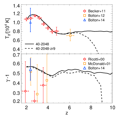
Figure 1: The two thermal histories used in the Sherwood simulations. The reference 40-2048 model corresponds to the Haardt & Madau (2012) ionising background (solid curve, reionisation at $z_{\rm r}=15$) with a small modification to the He$\,\rm\scriptstyle II\$photo-heating rate (see text for details). This is tuned to match observational constraints on the IGM temperature at mean density, $T_{0}$ (upper panel), obtained from the Ly$\alpha$ forest (Becker et al., 2011; Bolton et al., 2012, 2014). The 40-2048-zr9 model is similar at $z<6$, but with later reionisation at $z_{\rm r}=9$. The lower panel displays the power-law index, $\gamma-1$, of the temperature-density relation, $T=T_{0}\Delta^{\gamma-1}$, compared to Ly$\alpha$ forest measurements at $2<z<4$ (Ricotti et al., 2000; McDonald et al., 2001; Bolton et al., 2014). Note that Becker et al. (2011) measure the IGM temperature at the (redshift dependent) characteristic gas density probed by the Ly$\alpha$ forest, $T({\bar{\Delta}})$, rather than the temperature at mean density, $T_{0}$. This characteristic density ranges from ${\bar{\Delta}}=1.2$–$5.7$ at $2\leq z\leq 5$ (see their table 3). The Becker et al. (2011) $T_{0}$ data points in the upper panel are thus obtained using the $\gamma-1$ evolution shown by the solid line in the lower panel, i.e. $T_{0}=T({\bar{\Delta}})/{\bar{\Delta}}^{\gamma-1}$.

Table 1: Summary of the Sherwood simulation suite. The models analysed in this work are listed in the upper part of the table. The naming convention in the first column, L-N-param, encodes the box size, $L$, in $\rm h^{-1}\,cMpc$, the cube root, $N$, of the gas particle number, and any parameters which have been varied from the reference run (40-2048). These are: wdm –warm dark matter consisting of a $3.5\rm\,keV$ thermal relic (Viel et al., 2013a); zr9 – rapid reionisation beginning at $z_{\rm r}=9$ (cf. $z_{\rm r}=15$ for the reference model); ps13 – models including a sub-resolution treatment for star formation and galactic outflows (Puchwein & Springel, 2013); ps13+agn – as for ps13 but with the addition of AGN feedback. Subsequent columns list the dark matter and gas particle masses in $h^{-1}M_{\odot}$, the gravitational softening length in comoving $h^{-1}\rm\,kpc$, the final redshift, $z_{\rm end}$, of the simulation, the choice of random seed for the initial conditions and comments on each model.

Name	$M_{\rm dm}$	$M_{\rm gas}$	$l_{\rm soft}$	$z_{\rm end}$	Seed	Comments
	$\rm[h^{-1}\,M_{\odot}]$	$\rm[h^{-1}\,M_{\odot}]$	$\rm\,[h^{-1}\,ckpc]$
40-2048	$5.37\times 10^{5}$	$9.97\times 10^{4}$	0.78	2	A	Reference model
40-2048-wdm	$5.37\times 10^{5}$	$9.97\times 10^{4}$	0.78	2	A	Warm dark matter, $3.5\rm\,keV$ thermal relic
40-2048-zr9	$5.37\times 10^{5}$	$9.97\times 10^{4}$	0.78	2	A	Ionising background at $z\leq 9$ only
80-2048	$4.30\times 10^{6}$	$7.97\times 10^{5}$	1.56	2	B
40-1024	$4.30\times 10^{6}$	$7.97\times 10^{5}$	1.56	2	A
40-1024-ps13	$4.30\times 10^{6}$	$7.97\times 10^{5}$	1.56	2	A	Puchwein & Springel (2013) winds
20-512	$4.30\times 10^{6}$	$7.97\times 10^{5}$	1.56	2	C
40-512	$3.44\times 10^{7}$	$6.38\times 10^{6}$	3.13	0	A
40-2048-ps13	$5.37\times 10^{5}$	$9.97\times 10^{4}$	0.78	5.2	A	Puchwein & Springel (2013) winds
20-1024	$5.37\times 10^{5}$	$9.97\times 10^{4}$	0.78	2	C
10-512	$5.37\times 10^{5}$	$9.97\times 10^{4}$	0.78	2	A
160-2048	$3.44\times 10^{7}$	$6.38\times 10^{6}$	3.13	2	C
80-1024	$3.44\times 10^{7}$	$6.38\times 10^{6}$	3.13	0	B
20-256	$3.44\times 10^{7}$	$6.38\times 10^{6}$	3.13	0	C
160-1024	$2.75\times 10^{8}$	$5.10\times 10^{7}$	6.25	2	C
80-512	$2.75\times 10^{8}$	$5.10\times 10^{7}$	6.25	0	B
80-512-ps13	$2.75\times 10^{8}$	$5.10\times 10^{7}$	6.25	0	B	Puchwein & Springel (2013) winds
80-512-ps13+agn	$2.75\times 10^{8}$	$5.10\times 10^{7}$	6.25	0	B	Puchwein & Springel (2013) winds and AGN
160-512	$2.20\times 10^{9}$	$4.08\times 10^{8}$	12.50	2	C
80-256	$2.20\times 10^{9}$	$4.08\times 10^{8}$	12.50	0	B

The Sherwood simulations are summarised in Table 1. These consist of 20 models that span almost four orders of magnitude in mass resolution and employ a variety of physics parameters. The simulations required a total of 15 million core hours to run on the Curie supercomputer in France at the Tré Grand Centre de Calcul, using up to 6912 cores per run. The eight models analysed in this work are listed in the upper part of the table – the other models will be described in detail elsewhere (see e.g. Keating et al., 2016).

All the simulations were performed with a modified version of the parallel Tree-PM SPH code P-Gadget-3, which is an updated and extended version of the publicly available Gadget-2 (Springel, 2005). The models use the best fit $\Lambda$CDM Planck+WP+highL+BAO cosmological parameters (Planck Collaboration et al., 2014), where $\Omega_{\rm m}=0.308$, $\Omega_{\Lambda}=0.692$, $h=0.678$, $\Omega_{\rm b}=0.0482$, $\sigma_{8}=0.829$ and $n=0.961$. A primordial helium fraction by mass of $Y_{\rm p}=0.24$ is assumed throughout. The simulations do not include metal line cooling. This is expected to have very little effect on the Ly$\alpha$ forest transmission as the metallicity of the low density IGM is very low (Viel et al., 2013b). Initial conditions were generated at $z=99$ on a regular grid using the N-GenIC code (Springel et al., 2005) using transfer functions generated by CAMB (Lewis et al., 2000). The single exception is the 40-2048-wdm model, where the linear matter power spectrum has been suppressed at small scales to correspond to a warm dark matter thermal relic with mass $3.5\rm\,keV$, consistent with lower limits inferred from the Ly$\alpha$ forest at $z>4$ (Viel et al., 2013a). The gravitational softening length is set to $1/25^{\rm th}$ of the mean interparticle spacing and the SPH kernel uses $64$ neighbour particles in all simulations. Three different random seeds were used to generate the initial conditions. The same seed was used for simulations with the same box size (see Table 1) so that the same large scale structures are present.

The photo-ionisation and photo-heating of the hydrogen and helium gas is calculated using the spatially uniform Haardt & Madau (2012) ionising background model. The gas is assumed to be optically thin and in ionisation equilibrium. Except in rare, highly overdense regions, this is expected to be a very good approximation for the post-reionisation IGM at $z\leq 5$, when hydrogen is highly ionised and the mean free path for ionising photons is significantly larger than the typical separation of ionising sources (e.g. Worseck et al., 2014). However, inhomogeneous He$\,\rm\scriptstyle II\$reionisation may affect the gas temperatures at $z<4$, which is important for line widths but of secondary importance to the transmitted Ly$\alpha$ flux (we discuss this further in Section 3.5). The ionisation fractions are obtained following the method outlined by Katz et al. (1996), but with the case-A recombination rates from Verner & Ferland (1996), the dielectric He$\,\rm\scriptstyle I\$recombination rate from Aldrovandi & Pequignot (1973), collisional ionisation rates from Voronov (1997), collisional excitation cooling rates from Cen (1992), the bremsstrahlung cooling rate from Theuns et al. (1998) and the inverse Compton cooling rate from Weymann (1966), for free electrons scattering off cosmic microwave background photons with temperature $T_{\rm CMB}=2.73\rm\,K\,(1+z)$. A small modification to the He$\,\rm\scriptstyle II\$photo-heating rate, $\epsilon_{\rm HeII}=1.7\epsilon_{\rm HeII}^{\rm HM12}$ for $2.2<z<3.4$, is applied to match observational measurements of the IGM temperature at mean density, $T_{0}$, inferred from the curvature of Ly$\alpha$ forest absorption lines (Becker et al., 2011). A boost to the IGM temperature from non-equilibrium and radiative transfer effects during He$\,\rm\scriptstyle II\$reionisation is expected at these redshifts (Abel & Haehnelt, 1999; McQuinn et al., 2009; Puchwein et al., 2015).

The Haardt & Madau (2012) model furthermore results in the IGM being quickly reionised at $z_{\rm r}=15$. The most important effect this choice has on the Ly$\alpha$ forest at $z<5$ is to alter the pressure smoothing scale of gas in the simulations (e.g. Gnedin & Hui, 1998; Pawlik et al., 2009; Kulkarni et al., 2015); gas which has been ionised and heated later will have had less time to dynamically respond to the change in pressure. We thus also consider an alternative model, 40-2048-zr9, where the Haardt & Madau (2012) background has been modified to reionise the IGM at $z_{\rm r}=9$ but retains a similar evolution in the gas temperature at $z<6$. This later reionisation model is in better agreement with the latest measurement of the Thomson scattering optical depth for cosmic microwave background photons, which is consistent with instantaneous reionisation at $z_{\rm r}=8.8^{+1.7}_{-1.4}$ (Planck Collaboration et al., 2015). A comparison of the reference (40-2048) and 40-2048-zr9 thermal histories to observational measurements of the power-law IGM temperature-density relation, $T=T_{0}\Delta^{\gamma-1}$, where $\Delta=\rho/\langle\rho\rangle$ is the gas density relative to the background density (Hui & Gnedin, 1997; McQuinn & Upton Sanderbeck, 2016), is displayed in Fig. 1. We note that a fully self-consistent treatment of pressure smoothing would require radiation hydrodynamical simulations that model patchy reionisation (e.g. Pawlik et al., 2015), but these are too computationally expensive at present for modelling the $2\leq z\leq 5$ Ly$\alpha$ forest at high resolution. However, we do not expect these differences to be large, particularly at $z<5$; thermal pressure dominates over any hydrodynamical response of the gas to passing cosmological ionisation fronts, which can have velocities approaching a significant fraction of the speed of light (see also Finlator et al., 2012). The dynamical effects of He$\,\rm\scriptstyle II\$reionisation at $z\simeq 3$ are also at the few per cent level in dense regions when compared to simulations performed in the optically thin limit (Meiksin & Tittley, 2012).

Star formation is not followed in most of the simulations. Instead, gas particles with temperature $T<10^{5}\rm\,K$ and an overdensity $\Delta>1000$ are converted to collisionless particles (Viel et al., 2004b), resulting in a significant increase in computation speed at the expense of removing cold, dense gas from the model. This choice has a minimal effect on the low column density absorption systems probed by the Ly$\alpha$ forest. We do, however, perform some simulations with the star formation and energy-driven outflow model of Puchwein & Springel (2013) to investigate this further. The star formation prescription in this model follows Springel & Hernquist (2003), although it assumes a Chabrier rather than a Salpeter initial mass function. This increases the available supernovae feedback energy by a factor of $\sim 2$. Furthermore, rather than assuming a constant value of the wind velocity $v_{w}$, it scales with the escape velocity of the galaxy. The mass outflow rate in units of the star formation rate is then computed from the wind velocity and the available energy, i.e. it scales as $~{}v_{w}^{-2}$. This increased mass loading in low mass galaxies results in a much better agreement with the observed galaxy stellar mass function below the knee at low redshift, as well as in a suppression of excessive high-redshift star formation. Good agreement with the observed $z\sim 6$ galaxy stellar mass function is obtained (Keating et al., 2016). The wind and star formation model parameters are the same as in the S15 run of Puchwein & Springel (2013). The simulations discussed in this work do not include feedback from active galactic nuclei (AGN), although we have performed one low resolution run (80-512-ps13+agn) with the AGN feedback model described in Puchwein & Springel (2013) for examining the Ly$\alpha$ forest at $z<2$. AGN feedback is expected to impact on Ly$\alpha$ forest transmission statistics at the $5$–$10$ per cent level at $z=2.25$, but has a substantially smaller effect on the Ly$\alpha$ forest at higher redshift (Viel et al., 2013b).

Finally, we note that Ly$\alpha$ forest statistics are predominantly sensitive to low density gas ($\Delta\la 10$), and differ at only the $\sim 5$ per cent level between “standard” SPH used in this work and moving-mesh (Bird et al., 2013) or grid based codes (Regan et al., 2007). Uncertainties associated with high resolution observational measurements of the Ly$\alpha$ forest are typically similar to or larger than this, and at present this is not expected to significantly alter our conclusions.

2.2 Mock Ly$\alpha$ forest spectra

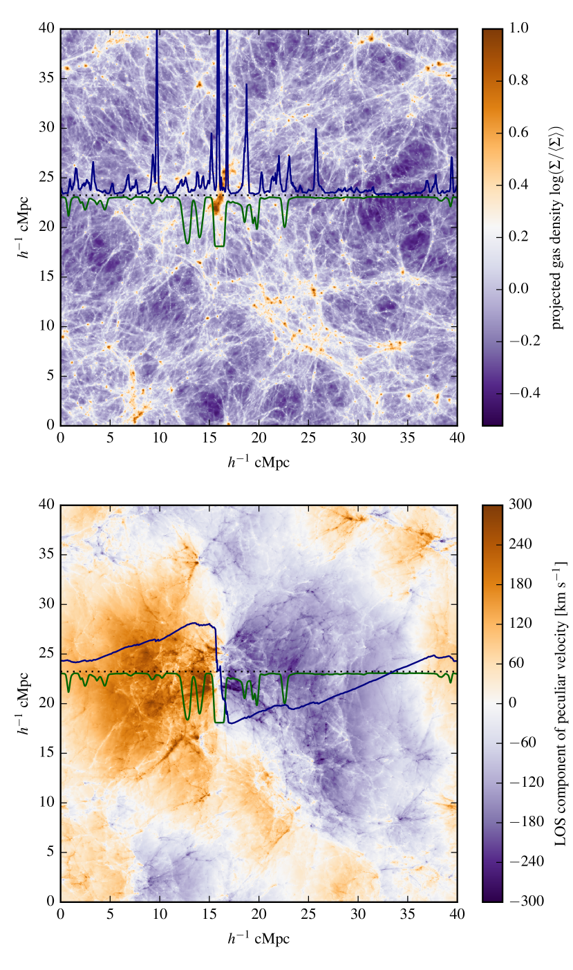
Figure 2: Projections of the proper gas density (upper panel) and the component of the peculiar velocity along the horizontal axis (lower panel) in the y-z plane of the 40-2048-zr9 simulation at $z=2$. The projection is performed along the entire box length of $40h^{-1}\,\rm cMpc$. Neutral hydrogen that traces the web-like distribution of gas in the upper panel is responsible for the absorption lines observed in the Ly$\alpha$ forest. This is illustrated by the horizontal dotted line, which marks the location of the line of sight corresponding to the Ly$\alpha$ absorption spectrum shown in green. The superimposed blue curves display the corresponding line of sight gas density (upper panel) and peculiar velocity (lower panel). Note the peculiar velocities shown by the blue curve are scaled such that the distance from the dotted line corresponds to the shift between real and redshift space along the line of sight.

Mock Ly$\alpha$ absorption spectra were extracted on-the-fly at redshift intervals of $\Delta z=0.1$ from all simulations. At each redshift, 5000 lines of sight with 2048 pixels were drawn parallel to each of the box axes ($x$, $y$ and $z$) on regularly spaced grids of $50^{2}$, $40^{2}$ and $30^{2}$, respectively. The gas density, H$\,\rm\scriptstyle I\$fraction, H$\,\rm\scriptstyle I\$weighted temperature and H$\,\rm\scriptstyle I\$weighted peculiar velocities were extracted following Theuns et al. (1998). The H$\,\rm\scriptstyle I\$Ly$\alpha$ optical depth along each line of sight, $\tau_{\rm HI}^{\alpha}$, was computed using the Voigt profile approximation provided by Tepper-García (2006). The transmitted flux in each pixel is then $F=e^{-\tau_{\rm HI}^{\alpha}}$.

An example mock Ly$\alpha$ forest spectrum and projections of the gas density and the component of the peculiar velocity along the horizontal axis in the 40-2048-zr9 model at $z=2$ are displayed in Fig. 2. The Ly$\alpha$ absorption lines arise from mildly overdense regions at this redshift, although the absorption features are typically offset from the physical location of the gas. This is because peculiar velocity gradients associated with structure formation impact on the location of the Ly$\alpha$ absorption features in velocity space. For example, the high density peaks at $10h^{-1}\rm\,cMpc$ and $25h^{-1}\rm\,cMpc$ along the horizontal axis correspond to the absorption features at approximately $12h^{-1}\rm\,cMpc$ and $23h^{-1}\rm\,cMpc$. These density peaks are associated with the filaments in the simulation volume. The most massive halo is located near the centre of the gas density projection in the upper panel of Fig. 2, with a dark matter mass of $2.4\times 10^{13}h^{-1}M_{\odot}$. The component of the peculiar velocity along the line of sight clearly shows gravitational infall around this high density region; positive (orange) peculiar velocities indicate gas that is moving from left to right, whereas negative (blue) velocities show gas that is moving from right to left.

Further comparison of the simulations to observations requires matching the properties of the observational data as closely as possible (Rauch et al., 1997; Meiksin et al., 2001). Throughout this paper we follow the standard practice of rescaling the optical depth in each pixel of the mock spectra by a constant factor to match the observed evolution of the Ly$\alpha$ forest effective optical depth, $\tau_{\rm eff}(z)=-\ln\langle F\rangle$ (Theuns et al., 1998; Bolton et al., 2005; Lukić et al., 2015). Here $\langle F\rangle=\langle f_{\rm obs}/C_{\rm est}\rangle$ is the mean Ly$\alpha$ forest transmission, $f_{\rm obs}$ is the observed flux in a resolution element of the background quasar spectrum and $C_{\rm est}$ is the corresponding estimate for the continuum level.

There are a wide range of effective optical depth measurements quoted in the literature (e.g. Kim et al., 2002; Bernardi et al., 2003; Schaye et al., 2003; Faucher-Giguère et al., 2008b; Pâris et al., 2011; Becker et al., 2013). In this work, when comparing simulations directly to published observational data sets we therefore always rescale to match the $\tau_{\rm eff}$ quoted in the publication where the observations were first presented. If we instead are comparing one simulation to another without reference to any observational measurements, we then adopt the following form for the redshift evolution of $\tau_{\rm eff}$ (Viel et al., 2013a):

$$\tau_{\rm eff}(z)=\left\{\begin{array}[]{cl}1.274\left(\frac{1+z}{5.4}\right)^{2.90}-0.132,&2\leq z\leq 4.4,\\ 1.142\left(\frac{1+z}{5.4}\right)^{4.91},&4.4<z\leq 5.\end{array}\right.$$ (3)

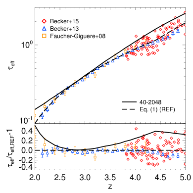
Figure 3: Upper panel: Observational measurements of the Ly$\alpha$ forest effective optical depth with redshift from Faucher-Giguère et al. (2008b) and Becker et al. (2013, 2015). The solid curve shows the redshift evolution in the 40-2048 simulation, obtained from mock spectra with a total path length of $10^{5}h^{-1}\rm\,cMpc$. The dashed curve, which more closely represents the data, is given by Eq. (3). Lower panel: The simulated and observational data relative to Eq. (3).

The fit at $z\leq 4.4$ corresponds to eq. (5) in Becker et al. (2013), with a steeper redshift evolution at $4.4<z<5$ similar to Fan et al. (2006). A comparison of Eq. (3) to the unscaled $\tau_{\rm eff}(z)$ from the reference model and observational data is displayed in Fig. 3. As already pointed out by Puchwein et al. (2015), the Haardt & Madau (2012) ionising background overestimates $\tau_{\rm eff}$ at $2<z<2.5$ and $z>4$. In order for the 40-2048 model to match Eq. (3), we find the H$\,\rm\scriptstyle I\$photo-ionisation rate, $\Gamma_{\rm HI}$, predicted by the Haardt & Madau (2012) model must be increased by $[87,\,3,\,47,\,65]$ per cent at $z=[2,\,3,\,4,\,5]$, corresponding to $\Gamma_{\rm HI}=[1.76,\,0.86,\,0.83,\,0.71]\times 10^{-12}\rm\,s^{-1}$. For a more detailed study of the H$\,\rm\scriptstyle I\$photo-ionisation rate at $2<z<5$ that includes an analysis of systematic uncertainties, see Becker & Bolton (2013).

Once rescaled to match the appropriate $\tau_{\rm eff}$, all mock spectra are convolved with a Gaussian instrument profile with a Full Width Half Maximum (FWHM) of $7\rm\,km\,s^{-1}$, typical of high resolution ($R\sim 40\,000$) Ly$\alpha$ forest observations obtained with echelle spectrographs. The spectra are rebinned onto $3\rm\,km\,s^{-1}$ pixels and uniform, Gaussian distributed noise is added. We adopt a signal-to-noise ratio of $\rm S/N=50$ per pixel unless otherwise stated, typical of the high resolution data sets we compare to.

The final adjustment we make to the mock spectra is a correction to the effective optical depth arising from systematic bias in the continuum level, $C_{\rm est}$, estimated in the observational data. This correction also changes the shape of the transmitted flux distribution and Ly$\alpha$ absorption lines. Identifying the continuum level in the Ly$\alpha$ forest becomes challenging toward higher redshift as the effective optical depth increases. The continuum may be placed too low on the observational data if the Ly$\alpha$ forest is optically thick, and there can also be large scale variations in the continuum placement along individual spectra. Faucher-Giguère et al. (2008b) quantify this bias by manually fitting the continuum, $C_{\rm est}$, on mock Ly$\alpha$ forest spectra where the true continuum, $C_{\rm true}$, has been deliberately hidden. This yields an estimate for a continuum correction $C_{\rm corr}=C_{\rm est}/C_{\rm true}$. In this work, unless otherwise stated we follow Faucher-Giguère et al. (2008b) and adopt their estimate for the mean continuum error at $2\leq z\leq 4$

$$C_{\rm corr}(z)=1-1.58\times 10^{-5}(1+z)^{5.63}.$$ (4)

As Faucher-Giguère et al. (2008b) do not determine $C_{\rm corr}$ at $z>4.5$, when comparing to observational data at $z=5$ in this work we instead follow Viel et al. (2013a) and estimate a maximum correction of $C_{\rm corr}=0.8$. We forward model this continuum bias by applying $C_{\rm corr}$ to mock spectra where the “true” continuum is already known. We use an iterative procedure where the optical depths in each pixel are first rescaled to match the observed $\tau_{\rm eff}$, the resolution and noise properties of the mock spectra are adjusted and finally the continuum bias correction is applied as $e^{-\tau_{\rm HI}^{\alpha}}/C_{\rm corr}$, again for each pixel (see also Rauch et al., 1997; Meiksin et al., 2001). This procedure is repeated until convergence on the required $\tau_{\rm eff}$ is achieved. Results from mock spectra where this procedure has been applied have labels appended with “cc” throughout.

An example of the continuum correction is displayed in Fig. 4. The mock spectra recover to the true continuum level ($F=1$) less frequently toward higher redshift as $\tau_{\rm eff}$ increases, hence the tendency to place the continuum too low when performing a blind normalisation. Note, however, Eq. (4) is model dependent. If there is missing physics in the simulations, for example volumetric heating which raises the temperature (and hence transmission) in underdense intergalactic gas (Puchwein et al., 2012; Lamberts et al., 2015), this may reduce the continuum bias estimated from the models.

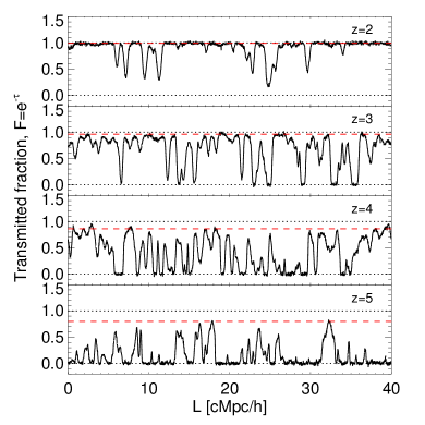
Figure 4: Mock Ly$\alpha$ forest spectra drawn from the reference 40-2048 simulation at $z=2,\,3,\,4$ and $5$. The spectra have been processed to resemble high resolution observational data (see text for details). The red dashed lines display the redshift dependent continuum correction we adopt in this work, given by Eq. (4).

Lastly, to estimate the expected sample variance in the observational data, we follow Rollinde et al. (2013) and bootstrap resample the simulated data with replacement over the observed absorption path length. The absorption path length interval, $\Delta X$, is related to the redshift interval by (Bahcall & Peebles, 1969)

$$\Delta X=\frac{(1+z)^{2}}{(\Omega_{\rm m}(1+z)^{3}+\Omega_{\Lambda})^{1/2}}\Delta z.$$ (5)

We bootstrap with replacement 1000 times over a total path length of $10^{5}h^{-1}\rm\,cMpc$, corresponding to $5000$ sight-lines from the smallest simulation box size considered in this work, $20h^{-1}\rm\,cMpc$. For convenience, we also provide the values of $\Delta X$ and $\Delta z$ that correspond to the box size of our reference model, 40-2048, in Table 2.

Table 2: Equivalent values for $L=40h^{-1}\rm\,cMpc$ – the box size of our reference model – expressed in terms of the redshift interval $\Delta z$, the absorption length interval $\Delta X$, the distance $R=L/h(1+z)$ in proper Mpc, and velocity $v_{\rm H}=H(z)R$ in $\rm km\,s^{-1}$.

z	$\Delta z$	$\Delta X$	$R$	$v_{\rm H}$
			[pMpc]	$[\rm km\,s^{-1}]$
2.0	0.040	0.120	19.7	4002
2.1	0.042	0.128	19.0	4053
2.5	0.050	0.163	16.9	4260
2.7	0.054	0.183	15.9	4364
3.0	0.060	0.213	14.7	4517
3.9	0.081	0.320	12.0	4961
4.0	0.084	0.334	11.8	5008
5.0	0.109	0.480	9.8	5466

3 Results

3.1 The transmitted flux distribution

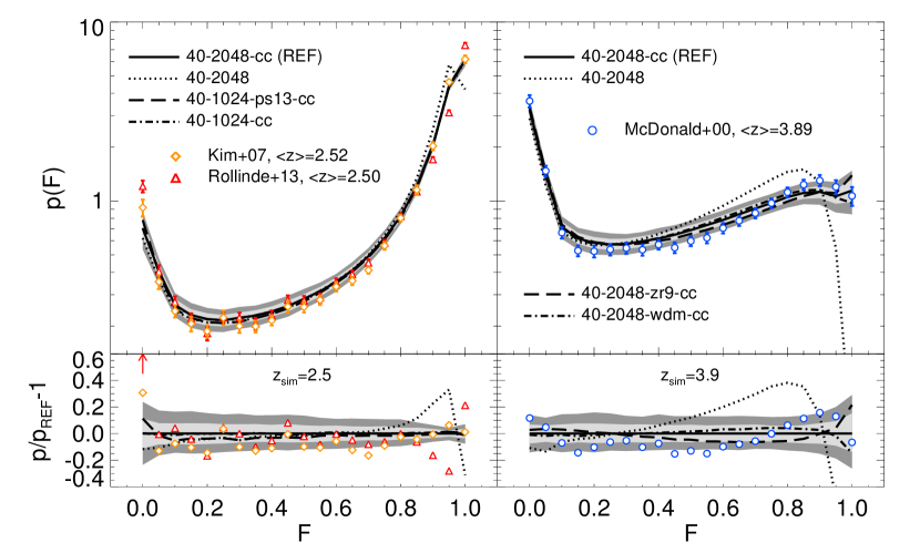
Figure 5: Upper panels: The transmitted flux PDF at $z\simeq 2.5$ (left) and $z\simeq 3.9$ (right). The observational data are from Kim et al. (2007), Rollinde et al. (2013) and McDonald et al. (2000). The solid curves correspond to the reference model after rescaling the effective optical depth to $\tau_{\rm eff}=0.227$ $(0.744)$ at $z=2.5$ $(z=3.9)$, and applying a redshift dependent continuum correction using Eq. (4) with a small adjustment at $z=3.9$ (see text for details). The grey shaded regions display the $1\sigma$ and $2\sigma$ uncertainties obtained when bootstrap resampling an absorption path length of $\Delta X=6.2$ ($z=2.5$) and $\Delta X=4.5$ ($z=3.9$) from a simulated path length of $10^{5}h^{-1}\rm cMpc$. The dotted curves in both panels show the reference model without the continuum correction. The effect of star formation and galactic winds may be assessed by comparing the dashed and dot-dashed curves in the left panel. The effect of a $3.5\rm\,keV$ warm dark matter particle and reionisation at $z_{\rm r}=9$ is shown in the right panel. Lower panels: The simulated and observational data (without the $1\sigma$ error bars) relative to the reference model. Upward pointing arrows indicate data points which lie outside the range of the ordinate.

We first examine the probability distribution function (PDF) of the transmitted flux. This has been examined in detail in the existing literature at $z<3$ (McDonald et al., 2000; Lidz et al., 2006; Kim et al., 2007; Calura et al., 2012; Rollinde et al., 2013; Lee et al., 2015), where discrepancies between hydrodynamical simulations and the observational data have been highlighted (Bolton et al., 2008, 2014; Tytler et al., 2009; Viel et al., 2009). These differences may be due in part to missing physics in the simulations; Bolton et al. (2008) noted the PDF measured by Kim et al. (2007) is in better agreement with models where underdense gas is hotter than usually expected. Rorai et al. (2016, submitted) have recently obtained a similar result in an analysis of the ultra-high signal-to-noise spectrum ($\rm S/N\simeq 280$ per pixel) of quasar HE0940$-$1050. A correction for continuum bias (Lee, 2012) and underestimated sample variance (Rollinde et al., 2013) can also assist with alleviating the tension between simulations and the observed PDF.

In the left panel of Fig. 5 we compare the PDF from the simulations to observational measurements from Kim et al. (2007) and Rollinde et al. (2013) at $z\simeq 2.5$. Both observational data sets consist of 18 high resolution spectra obtained with the Very Large Telescope (VLT) using the Ultraviolet and Visual Echelle Spectrograph (UVES) (Dekker et al., 2000). A total of 14 spectra are common to both compilations, but the spectra have been reduced independently. The data in the Kim et al. (2007) redshift bin displayed in Fig. 5 spans $2.37\leq z\leq 2.71$ and has a total absorption path length of $\Delta X=6.2$. Rollinde et al. (2013) use the same redshift bin with $\Delta X=5.3$. The mock spectra have been scaled to match the effective optical depth from Kim et al. (2007), $\tau_{\rm eff}=0.227$. The spectra are then convolved with a Gaussian instrument profile, rebinned and noise is added as described in Section 2.2.

The majority of the observational data at $z=2.5$ are within the $2\sigma$ range estimated from the simulations, although around half of the bins lie more than $1\sigma$ below the model average (see also fig. 6 in Rollinde et al., 2013). An isothermal ($\gamma-1=0$) temperature-density relation improves the agreement at $0.1<F<0.8$ (cf. fig. 4 in Bolton et al., 2014), suggesting that hot underdense gas may be missing from the simulations. The most significant discrepancies, however, are at $F>0.8$ and $F=0$. As noted by Lee (2012) the continuum correction helps improve agreement with the Kim et al. (2007) data at $F>0.8$ – the reference model with no continuum correction is shown by the dotted curve. Significant differences with the Rollinde et al. (2013) measurements at $F\geq 0.85$ remain, although we find a further 3 per cent change to the continuum correction in Eq. (4) improves the agreement.

In contrast, at $F=0$ the star formation and galactic winds implementation and the signal-to-noise ratio are important. This is evident from the effect of the Puchwein & Springel (2013) outflow model, shown by the dashed curve, which increases the number of saturated pixels by 10 per cent. This additional absorption is associated with saturated Ly$\alpha$ absorption lines with $N_{\rm HI}>10^{14.5}\rm\,cm^{-2}$. We demonstrate later that these systems are more common in the model with star formation and outflows (see Section 3.4). As pointed out by Kim et al. (2007), the signal-to-noise of the data also impacts on the PDF quite strongly at $F<0.1$. Differences in the PDF can be up to a factor of two between $\rm S/N=25$ and $\rm S/N=100$ (see their fig. 7), with higher $\rm S/N$ increasing the PDF at $F=0$ and decreasing it at $F=0.1$. A more detailed treatment of the noise may therefore also assist with improving agreement here.

The right panel of Fig. 5 compares the reference model to measurements from McDonald et al. (2000) at higher redshift, $z=3.9$. The McDonald et al. (2000) measurements are derived from eight high resolution spectra obtained with the High Resolution Echelle Spectrometer (HIRES) on the Keck telescope (Vogt et al., 1994). The total path length for the McDonald et al. (2000) data is $\Delta X=4.5$ and their redshift bin spans $3.39\leq z\leq 4.43$. The mock spectra have been scaled to match the McDonald et al. (2000) effective optical depth, $\tau_{\rm eff}=0.744$, and processed as before to resemble the data.

Without any continuum correction the reference model (dotted curve) fails to reproduce the shape of the PDF. We correct for this using Eq. (4) with a small modification, where $C_{\rm corr}$ is adjusted upwards by $0.02$ to $C_{\rm corr}=0.9$. This significantly improves the agreement (solid curve), decreasing the number of pixels by $30$–$40$ per cent at $F=0.8$. Note, however, that at $z=4$ the simulations will still underpredict the number of pixels close to the continuum by $\sim 10$ per cent due to poor mass resolution in the low density regions probed by the Ly$\alpha$ forest at high redshift (see the convergence tests in the Appendix). A similar convergence rate was noted by Lukić et al. (2015) using the Nyx code, suggesting that correcting for box size effects would require a value of $C_{\rm corr}$ closer to the value predicted by Eq. (4) to achieve a similar level of agreement. However, given the relatively small path length of the McDonald et al. (2000) data, updated measurements of the PDF at $z>3.5$ would be very useful for testing this further.

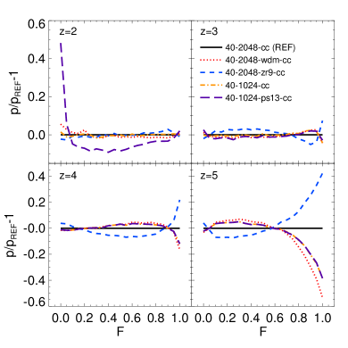
Figure 6: The transmitted flux PDF at $z=2,\,3,\,4$ and $5$ relative to the reference model (40-2048-cc). The effect of different model parameters on the PDF is displayed, including a $3.5\rm\,keV$ warm dark matter particle (red dotted curve), rapid reionisation at $z_{\rm r}=9$ (blue short dashed curve) and star formation and galactic winds (purple long dashed curve). The latter model is at lower resolution, and should be directly compared to the 40-1024-cc model (orange dot-dashed curve). The effective optical depth is scaled to match Eq. (3).

Finally, the dashed and dot-dashed curves in the right panel of Fig. 5 demonstrate models with later reionisation at $z_{\rm r}=9$ (40-2048-zr9-cc) or a $3.5\rm\,keV$ warm dark matter particle (40-2048-wdm-cc) impact on the PDF at the 5–10 per cent level at $z=3.9$. These differences are smaller than the effect of a plausible continuum correction, and largely disappear by $z<3$. On the other hand, star formation and galactic outflows have very little effect on the low density gas probed by the Ly$\alpha$ forest at $z\simeq 4$ (see also Theuns et al., 2002; Viel et al., 2013b). This may be observed more clearly in Fig. 6, which displays the ratio of the PDF to the reference model for a variety of model parameters at $z=2,\,3,\,4$ and $5$ after rescaling all models to have the same effective optical depth. In contrast, the effect of warm dark matter and pressure smoothing become increasingly important approaching high redshift but act in opposite directions, decreasing and increasing the fraction of high transmission regions, respectively.

3.2 The transmitted flux power spectrum

The power spectrum of the transmitted flux has been extensively used to constrain cosmological parameters with the Ly$\alpha$ forest (Croft et al., 1999, 2002; McDonald et al., 2000, 2006; Viel et al., 2004b, 2013a; Palanque-Delabrouille et al., 2013, 2015). A comparison of the simulations to measurements of the power spectrum at $z=2.1$ and $z=3.9$ is displayed in Fig. 7.

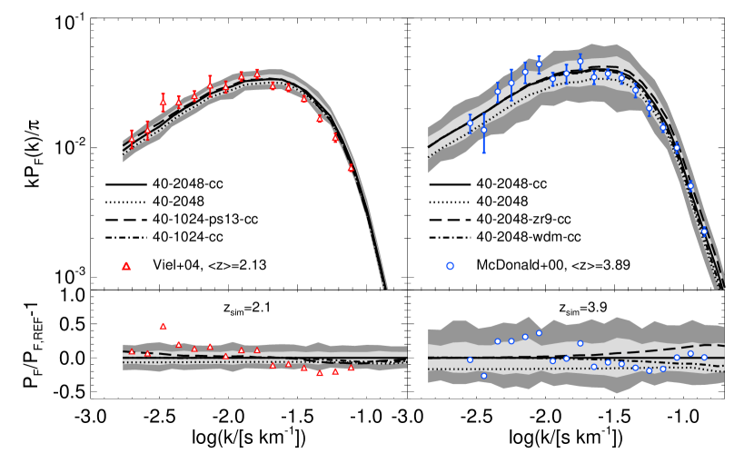
Figure 7: Upper panels: The power spectrum of the transmitted flux estimator $\delta_{\rm F}=F/\langle F\rangle-1$ at $z\simeq 2.1$ (left) and of the transmitted flux $F$ at $z\simeq 3.9$ (right), compared to observational data from Viel et al. (2004b) and McDonald et al. (2000). The solid curves correspond to the 40-2048 model after rescaling the effective optical depth to $\tau_{\rm eff}=0.180$ $(0.744)$ at $z=2.1$ $(z=3.9)$, and applying a redshift dependent continuum correction using Eq. (4) with a small adjustment at $z=3.9$ (see text for details). The grey shaded regions display the 68 and 95 per cent confidence intervals obtained when bootstrap resampling an absorption path length of $\Delta X=11.9$ ($\Delta X=4.5$) from a simulated path length of $10^{5}h^{-1}\rm cMpc$. The other curves are as described in Fig. 5. Lower panels: The simulations and observational data (excluding error bars) relative to the reference model 40-2048-cc.

The left panel of Fig. 7 compares the measurements of Viel et al. (2004b) at $\langle z\rangle=2.13$ to the models. The Viel et al. (2004b) data are obtained from 16 quasar spectra spanning the redshift bin $2<z<2.3$, selected from the VLT/UVES LUQAS (Large Sample of UVES Quasar Absorption Spectra) sample from Kim et al. (2004). The Viel et al. (2004b) power spectrum is computed using the estimator $\delta_{\rm F}=F/\langle F\rangle-1$. The absorption path length of these data is $\Delta X=11.9$ and our mock spectra are rescaled to correspond to $\tau_{\rm eff}=0.18$, consistent with the value of $\tau_{\rm eff}=0.17\pm 0.02$ quoted by Viel et al. (2004b). These authors inferred cosmological parameters by fitting the power spectrum in the range $-2.5<\log(k/\rm s\,km^{-1})<-1.5$, where systematic uncertainties due to continuum fitting, damped absorption systems and metal lines should be minimised.

We find the Sherwood simulations are in good agreement with the data, with the majority of the bins lying within $1$–$2\sigma$ of the models. The largest discrepancy is the data point at $\log(k/\rm s\,km^{-1})\simeq-2.5$, although the dashed curve corresponding to 40-1024-ps13-cc again indicates that star formation and outflows may improve agreement here. The larger number of high column density systems in this model increases the power by around 10 per cent at large scales, $\log(k/\rm s\,km^{-1})<-2$ (see also Viel et al., 2004a; McDonald et al., 2005). In contrast, the impact of the Puchwein & Springel (2013) star formation and winds at scales $\log(k/\rm s\,km^{-1})>-1.5$ is rather small; note that much of the difference relative to the reference run is due to the lower mass resolution of the 40-1024-ps13-cc model. Instead, hotter underdense gas can decrease power on small scales at this redshift, potentially improving agreement with the small scale measurements (see e.g. fig. 3 in Viel et al., 2004b). The continuum correction is small at $z=2.1$, but acts to increase power on all scales by $\sim 5$ per cent.

A higher redshift measurement at $\langle z\rangle=3.89$ from McDonald et al. (2000) is compared to the models in the right hand panel of Fig. 7. The mock spectra have been scaled to $\tau_{\rm eff}=0.744$, and the observational data, absorption path length and continuum correction are the same as those used for the McDonald et al. (2000) PDF measurement at the same redshift (see Section 3.1). The reference model is in excellent agreement ($1$–$2\sigma$) with data following the continuum correction, which increases power on all scales. Without this correction, however, the data points lie systematically above the model, particularly at scales $\log(k/\rm s\,km^{-1})<-1.5$. This suggests a careful treatment of the continuum placement is especially important for forward modelling high redshift Ly$\alpha$ forest data. Although the effect of star formation and galactic outflows is minimal at $z\simeq 4$ (see Fig. 9), a later reionisation at $z_{\rm r}=9$ results in less pressure smoothing and hence more power on scales $\log(k/\rm s\,km^{-1})>-1.7$. This indicates it should be possible to constrain the integrated thermal history during reionisation using the line of sight Ly$\alpha$ forest power spectrum at high redshift (Nasir et al., 2016). However, the magnitude of the effect at $z\simeq 4$ lies within the $1\sigma$ bootstrapped uncertainty for the McDonald et al. (2000) absorption path length. Either more quasar spectra or higher redshift data where the effect is stronger will assist here. Note also the opposite effect is observed for the warm dark matter model, with power reduced by around 10 per cent at scales $\log(k/\rm s\,km^{-1})\sim-1$. Again, however, this difference lies within the expected $1\sigma$ range for the rather small absorption path length of the McDonald et al. (2000) sample.

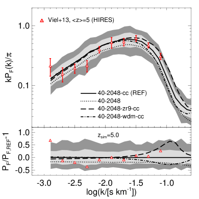
Figure 8: Upper panel: The power spectrum of the transmitted flux estimator $\delta_{\rm F}=F/\langle F\rangle-1$ at $z=5$, compared to observational data from Viel et al. (2013a) obtained with the Keck/HIRES spectrograph. The solid curve corresponds to the 40-2048-cc model with $\tau_{\rm eff}=1.76$. The grey shaded regions display the $1\sigma$ and $2\sigma$ uncertainties obtained when bootstrap resampling an absorption path length interval of $\Delta X=5.4$ from a simulated path length of $10^{5}h^{-1}\rm cMpc$. The dotted curve shows the 40-2048 model without the continuum correction. The effect of a $3.5\rm\,keV$ warm dark matter particle and rapid reionisation at $z_{\rm r}=9$ are shown by the dashed and dot-dashed curves. The mock spectra have been processed to match the resolution and signal-to-noise properties of the observational data (see text for details). Lower panel: The simulated and observational data (excluding error bars) relative to the reference model.

In Fig. 8 we also compare the simulations to the power spectrum at $\langle z\rangle=5$ presented by Viel et al. (2013a). These authors placed a lower limit on the possible mass of a warm dark matter thermal relic, $m_{\rm WDM}\geq 3.3\rm\,keV$ ($2\sigma$). The power spectrum measurement is based on an analysis of 14 quasar spectra with emission redshifts $4.48\leq z\leq 6.42$ obtained with Keck/HIRES. The redshift bin displayed here spans the redshift range $4.8<z<5.2$. The total path absorption path length is $\Delta X=5.4$ with a typical $\rm S/N=10$–$20$. The simulations have been rescaled to $\tau_{\rm eff}=1.76$, consistent with the lower $1\sigma$ bound on the best fit obtained by Viel et al. (2013a), and a uniform signal-to-noise of $\rm S/N=20$ is added to each pixel. Note that to obtain their warm dark matter constraints, Viel et al. (2013a) use the power spectrum over the range $-2.3\leq\log(k/\rm s\,km^{-1})\leq-1.1$.

As with the comparison at $z\simeq 3.9$, the continuum correction increases the power by around 20 per cent on all scales. The observations are again in very good agreement with the reference model; most lie within $1$–$2\sigma$ of the expected variance. It is also clear that the differences between the reference and late reionisation models are more apparent toward higher redshift, closer to the reionisation redshift and where the Ly$\alpha$ forest probes scales where structure is closer to the linear regime. Note, however, the mass resolution correction means the power on scales $\log(k/\rm s\,km^{-1})\simeq-1$ is still underestimated by around 10 per cent in this model (see the Appendix and Bolton & Becker, 2009; Viel et al., 2013a).

Finally, Fig. 9 displays the power spectrum for different model parameters at four different redshifts, where again all models are scaled to match Eq. (3). As for the PDF, the effect of star formation and galactic winds is significant at $z<3$, increasing the power on large scales due to the presence of additional high column density systems (see Section 3.4). Similarly, the effect of a $3.5\rm\,keV$ warm dark matter thermal relic and late reionisation are degenerate and have a dramatic effect on the power on small scales at high redshift (40–80 per cent), but only at the level of a few per cent at lower redshift.

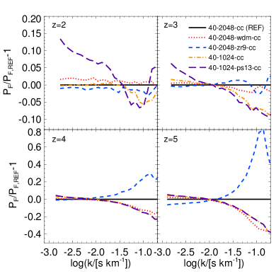
Figure 9: The power spectrum of the transmitted flux, $F$, at $z=2,\,3,\,4$ and $5$ relative to the reference model (40-2048-cc). The effect of different model parameters on the power spectrum is displayed, including a $3.5\rm\,keV$ warm dark matter particle (red dotted curve), rapid reionisation at $z_{r}=9$ (blue short dashed curve) and star formation and outflows (purple long dashed curve). The latter model is at lower resolution, and should be directly compared to the 40-1024-cc model (orange dot-dashed curve). The effective optical depth is scaled to match Eq. (3).

3.3 The standard deviation of the mean transmitted flux

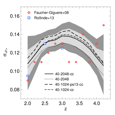
Figure 10: The standard deviation of the mean transmitted flux measured in $3\rm\,pMpc$ segments as a function of redshift. The red diamonds and blue squares are observational measurements from Faucher-Giguère et al. (2008b) and Rollinde et al. (2013). Simulation results are represented by the curves indicated in the panel. All simulation results, aside from the dotted curve, also have a redshift dependent continuum correction applied (see Eq. 4). The grey shaded regions correspond to the 68 and 95 per cent confidence intervals for the 40-2048 model, obtained when bootstrap resampling the Faucher-Giguère et al. (2008b) path length in each redshift bin from a total simulated path length of $10^{5}h^{-1}\rm\,cMpc$.

We next investigate the scatter in the mean transmission by comparing the standard deviation of the mean transmitted flux, $\sigma_{\langle F\rangle}$, to observational measurements from Faucher-Giguère et al. (2008b) and Rollinde et al. (2013) (the latter data set is described in Section 3.1). The Faucher-Giguère et al. (2008b) data consist of 86 high resolution quasar spectra obtained with the Echelle Spectrograph and Imager (ESI) and HIRES on the Keck telescope and the Magellan Inamori Kyocera Echelle (MIKE) spectrograph on the Magellan telescope. Our mock spectra are processed to match the best-fit power law to the effective optical depth from Faucher-Giguère et al. (2008b), $\tau_{\rm eff}=0.0018(1+z)^{3.92}$. Following these authors, at intervals of $\Delta z=0.2$ over the range $2\leq z\leq 4.2$ we compute the standard deviation of the mean transmitted flux, $\sigma_{\langle F\rangle}$, in segments of $3\rm\,pMpc$. We estimate the sample variance on this quantity by bootstrap resampling the observed path length from Faucher-Giguère et al. (2008b) (see their fig. 4) from a total path length of $10^{5}h^{-1}\rm\,cMpc$.

Fig. 10 shows the standard deviation peaks around $z=3$, and falls toward lower and higher redshift as proportionally more pixels lie either at the continuum ($F=1$) or are saturated ($F=0$). The 68 and 95 per cent confidence intervals for the continuum corrected reference model are indicated by the grey shaded regions. The simulations are in agreement with the data at $z<3$, but at $z>3$ three data points differ at more than $2\sigma$. It is unlikely these differences are attributable to star formation and galactic outflows. A comparison of the dot-dashed and dashed curves in Fig. 10 demonstrate the Puchwein & Springel (2013) variable winds model increases $\sigma_{\langle F\rangle}$ by $\sim 8$ per cent at $z=2$, but this difference diminishes toward higher redshift. In contrast, the impact of the continuum correction – indicated by the solid and dotted curves – is much larger. This acts to increase $\sigma_{\langle F\rangle}$ by distributing the pixels over a broader range of values. Lowering the continuum at $z=4.2$ by a further $10$ per cent, or placing the continuum too high by $5$ per cent at $z=3.2$ and $z=3.4$, leads to $2\sigma$ agreement with the data. This suggests that observational systematics may in part explain the discrepancy at $z>3$. We have verified the reference simulation is converged to within $2$–$3$ per cent with respect to box size and mass resolution over the redshift range we consider; further details are available in the Appendix.

3.4 The column density distribution function

In this section we now turn to compare our mock spectra to the results of a Voigt profile analysis of high resolution data using VPFIT (Carswell & Webb, 2014). The observational data are from Kim et al. (2013), which comprises 18 high resolution quasar spectra from the European Southern Observatory (ESO) VLT/UVES archive with a typical signal-to-noise per pixel of $\rm S/N=35$–$50$. We compare to the Ly$\alpha$ forest observed in two redshift bins at $\langle z\rangle=2.13$ and $\langle z\rangle=2.72$, spanning $1.9<z<2.4$ and $2.4<z<3.2$ with a total absorption path length of $\Delta X=12.5$ and $\Delta X=10.5$, respectively. Absorption features within $\pm 50\rm\,\AA$ of damped Ly$\alpha$ absorbers are ignored in these data, as well as all Ly$\alpha$ lines within $5000\rm\,km\,s^{-1}$ of the quasar systemic redshift to avoid the proximity effect. We use the H$\,\rm\scriptstyle I\$column densities, $N_{\rm HI}$, and velocity widths, $b_{\rm HI}$, obtained from fits to the Ly$\alpha$ absorption profiles only, enabling a straightforward comparison to the mock Ly$\alpha$ forest spectra. We note, however, that both Kim et al. (2013) and Rudie et al. (2013) provide alternative fits for saturated lines, $N_{\rm HI}>10^{14.5}\rm\,cm^{-2}$, obtained using higher order Lyman series transitions.

The mock spectra are rescaled to match the effective optical depth evolution from Kim et al. (2007), $\tau_{\rm eff}=0.143$ $(0.273)$ at $z=2.1$ ($z=2.7$), and processed as described in Section 2.2. Voigt profiles were then fitted to $20h^{-1}\rm\,cMpc$ segments using VPFIT. All lines within $100\rm\,km\,s^{-1}$ of the start and end of each segment were ignored to avoid edge artefacts. We use the same procedure followed by Kim et al. (2013) when performing this analysis, thus minimising any possible biases introduced by the Voigt profile decomposition process.

We first examine the column density distribution function (CDDF), defined as the number of absorption lines per unit column density per unit absorption path length

$$f(N_{\rm HI},X)=\frac{\partial^{2}n}{\partial N_{\rm HI}\partial X}.$$ (6)

We compare to the Kim et al. (2013) CDDF measurements for absorption lines in the Ly$\alpha$ forest with column densities in the range $10^{12.3}\rm\,cm^{-2}\leq N_{\rm HI}\leq 10^{16.8}\rm\,cm^{-2}$. Note, however, that at $N_{\rm HI}<10^{12.7}\rm\,cm^{-2}$ the CDDF will be affected by incompleteness. Absorption lines that are optically thick to Lyman continuum photons (i.e $N_{\rm HI}>10^{17.2}\rm\,cm^{-2}$) will not be captured in our optically thin simulations, and we do not consider these further here. Recent hydrodynamical simulations that incorporate corrections for self-shielding have been shown to capture the normalisation and shape of the CDDF in this regime (Altay et al., 2011; Rahmati et al., 2013).

Fig. 11 displays the observed CDDF in comparison to simulations at $z=2.1$ (left) and $z=2.7$ (right). The agreement, particularly for unsaturated lines with $10^{12.7}\rm\,cm^{-2}<N_{\rm HI}<10^{14.4}\rm\,cm^{-2}$ is remarkably good and is largely within the expected $1\sigma$ and $2\sigma$ bootstrapped uncertainties displayed by the grey shading. The dotted curve indicates the continuum correction acts to slightly decrease (increase) the number of weak (strong) lines. On the other hand, the simulations underestimate the number of lines at $N_{\rm HI}=10^{12.4}\rm\,cm^{-2}$ by $30$–$40$ per cent. The comparison between the solid and dot-dashed curves indicates the simulations are well converged with respect to mass resolution here (see also the Appendix). However, these low column density lines are strongly affected by the signal-to-noise of the data and misidentified metal lines. We have verified that lowering the signal-to-noise further decreases the number of weak lines identified. As our simulations do not include metals and adopt a uniform $\rm S/N=50$, this may in part account for the difference.

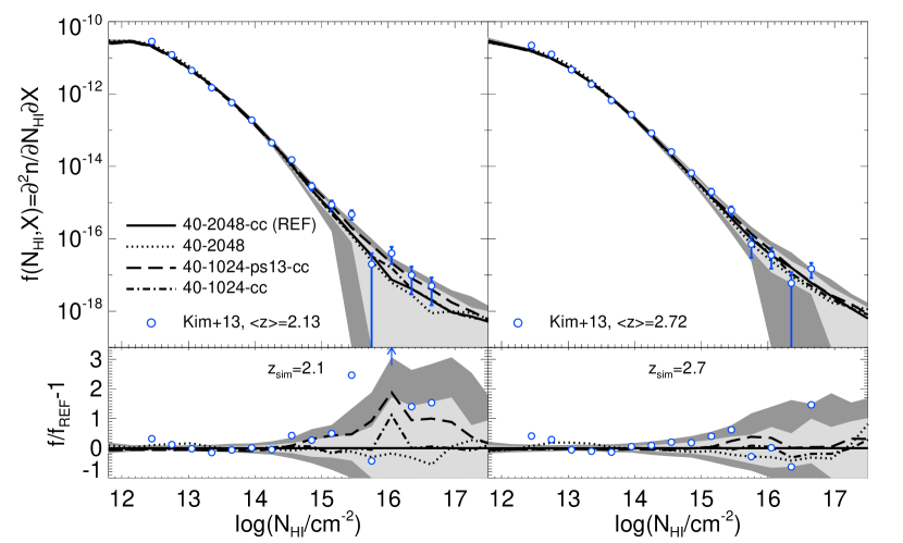
Figure 11: Upper panels: The Ly$\alpha$ forest column density distribution function compared to observational data from Kim et al. (2013) at $z\simeq 2.1$ (left) and $z\simeq 2.7$ (right). The solid curves correspond to the 40-2048-cc model after rescaling the effective optical depth to match Kim et al. (2007), $\tau_{\rm eff}=0.143$ ($0.273$) at $z=2.1$ ($z=2.7$), and applying the redshift dependent continuum correction from Eq. (4). The grey shaded regions display the 68 and 95 per cent confidence intervals obtained when bootstrap resampling an absorption path length interval of $\Delta X=12.5$ ($z=2.1$) and $\Delta X=10.5$ ($z=2.7$) from a simulated path length of $10^{5}h^{-1}\rm cMpc$. The dotted curve shows the 40-2048 model without the continuum correction. The effect of galactic winds may be assessed by comparing the dashed and dot-dashed curves. The mock spectra have been processed to broadly match the resolution and signal-to-noise properties of the observational data (see text for details). Lower panel: The simulated and observational data (excluding error bars) relative to the reference model. Upward pointing arrows indicate data points which lie outside the range of the ordinate.

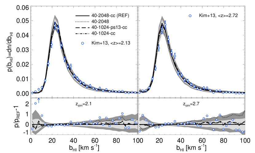
Figure 12: Upper panels: The distribution of velocity widths, $b_{\rm HI}$, for Ly$\alpha$ absorption lines compared to observational data from Kim et al. (2013) at $z=2.1$ (left) and $z=2.7$ (right). Only lines with $12.3\leq\log(N_{\rm HI}/\rm cm^{-2})\leq 17.0$ are included in this comparison. The simulation data, shown by the curves and grey shading, are as described in the caption of Fig. 11. Lower panels: The simulated and observational data (excluding error bars) relative to the reference model. Upward pointing arrows indicate data points which lie outside the range of the ordinate.

For saturated lines at $N_{\rm HI}\geq 10^{14.5}\rm\,cm^{-2}$, a much larger difference is seen for the model with the Puchwein & Springel (2013) star formation and galactic winds implementation at $z=2.1$. Comparing the dot-dashed and dashed curves suggest the incidence of saturated lines is underestimated by up to a factor of two for models which do not include sub-resolution treatments for galaxy formation physics and galactic outflows. This suggests the approximate scheme for removing cold $(T<10^{5}\rm\,K$), dense ($\Delta>1000$) gas used in our reference runs does not fully capture the incidence of saturated absorption systems at $z\simeq 2$. These differences are qualitatively consistent with the results from the PDF and power spectrum, where the observational data exhibit more saturated pixels and an increase in large scale power compared to the simulations at similar redshifts. In contrast, at $z=2.7$ the effect of star formation and galactic outflows on the CDDF is more modest and the incidence of saturated lines in the mock spectra is consistent with the observations. This indicates that the sensitivity of the Ly$\alpha$ forest to high density gas decreases toward higher redshift.

3.5 The velocity width distribution

The distribution of Ly$\alpha$ line velocity widths, $b_{\rm HI}$, from the Kim et al. (2013) observational data are displayed in Fig. 12. Only the velocity widths for absorbers with $10^{12.3}\rm\,cm^{-2}\leq N_{\rm HI}\leq 10^{17.0}\rm\,cm^{-2}$ are included in the distribution. The simulations are again in very good agreement with the data. In this case, the continuum correction acts to produce more (fewer) narrow (wide) lines. At $z=2.1$ there is a deviation at just over $2\sigma$ for the bin at $20\rm\,km\,s^{-1}$, although the peak of the simulated distribution matches the data. However, the main discrepancy at $z=2.1$ (and to a much lesser extent at $z=2.7$) is for lines with $b_{\rm HI}<10\rm\,km\,s^{-1}$. In combination with missing low column density lines in the CDDF, this again suggests misidentified metal line absorbers – which become more prevalent toward lower redshift – are responsible for the additional weak, narrow lines in the data. The excellent agreement with the shape of the distribution at $b_{\rm HI}>10\rm\,km\,s^{-1}$ indicates that the gas temperatures at this redshift are largely consistent with the observational data. This is expected given the models were tuned to match (independent) observational constraints on the IGM temperature (e.g. Fig. 1).

In the higher redshift bin, the agreement is also generally good. The peak of the velocity width distribution in the simulations is $3\rm\,km\,s^{-1}$ below the peak in the observed distribution, but remains consistent within the expected $2\sigma$ range. Two data points at $17\rm\,km\,s^{-1}$ and $20\rm\,km\,s^{-1}$ again deviate at more than $2\sigma$, possibly indicating the gas may be slightly too cold (by a few thousand degrees) in the model at this redshift. Additional heating from non-equilibrium ionisation effects during He$\,\rm\scriptstyle II\$reionisation may account for this small difference (Puchwein et al., 2015).

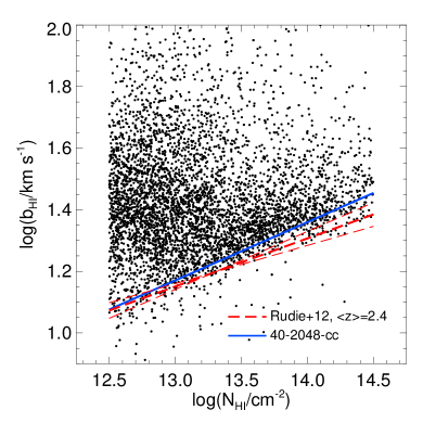
Figure 13: The $b_{\rm HI}-N_{\rm HI}$ plane at $z=2.4$, shown by the points, corresponds to $5\,000$ Voigt profiles which have been fitted to mock spectra from the reference model. The effective optical depth is scaled to match Eq. (3) and a redshift dependent continuum correction has been applied using Eq. (4). The signal to noise is $\rm S/N=89$, and the lines have been selected following the default criteria specified by Rudie et al. (2012). The lower envelope of this distribution may be compared to the observationally measured lower cut-off from Rudie et al. (2012). The thick red dashed line corresponds to their ”default” measurement, with the thin lines representing the $1\sigma$ uncertainty. For comparison, the blue line shows the lower cut-off measured in the same way from the simulation data.

As a further consistency check, in Fig. 13 we examine the $b_{\rm HI}$–$N_{\rm HI}$ plane at $z=2.4$ in the simulations. This is compared to the lower envelope of the $b_{\rm HI}$–$N_{\rm HI}$ plane measured by Rudie et al. (2012) from simultaneous fits to Ly$\alpha$ and Ly$\beta$ absorption in a sample of 15 high signal-to-noise ($\rm S/N\simeq 50$–$200$) quasar spectra obtained with Keck/HIRES. Their Voigt profile analysis consists of $5758$ absorbers with $12.0<\log(N_{\rm HI}/\rm cm^{-2})<17.2$ and a mean redshift of $\langle z\rangle=2.37$. Rudie et al. (2012) fit a power-law to the lower envelope of the $b_{\rm HI}$–$N_{\rm HI}$ distribution for $12.5<\log(N_{\rm HI}/\rm cm^{-2})<14.5$ following the method of Schaye et al. (1999). By comparing this power-law relation to models, it is possible to infer the amplitude and slope of the temperature density relation, $T=T_{0}\Delta^{\gamma-1}$. Bolton et al. (2014) performed a detailed reanalysis of this measurement, finding $T_{0}=10000^{+3200}_{-2100}\rm\,K$ and $\gamma-1=0.54\pm 0.11$.

We scale the effective optical depth of mock spectra at $z=2.4$ to match Eq. (3) and add a uniform signal-to-noise per pixel of $\rm S/N=89$, corresponding to the average of the Rudie et al. (2012) data set. Lines are selected following the default criteria described by these authors. The resulting $b_{\rm HI}$–$N_{\rm HI}$ plane in Fig. 13 is broadly consistent with the Rudie et al. (2012) measurement, shown by the red dashed line, although note again that from Fig. 1 this should be expected. The blue line displays the lower cut-off measured from the mock data in the same way as Rudie et al. (2012). A column density of $N_{\rm HI}\simeq 10^{12.95}\rm\,cm^{-2}$ corresponds to the mean background density at this redshift (Bolton et al., 2014), suggesting that the value of $T_{0}=11735\rm\,K$ used in the 40-2048 simulation is in reasonable agreement with the observations. On the other hand, the slightly steeper slope relative to the red dashed line indicates that reducing the value of $\gamma-1=0.57$ used in the simulation by $\Delta\gamma\sim 0.05$–$0.1$ may provide better agreement with the observational data at $z=2.4$. As discussed in Bolton et al. (2014) and Rorai et al. (2016, submitted), however, this agreement does not rule out the possibility that underdense gas in the IGM is hotter than expected from a simple extrapolation of this temperature-density relation to $\Delta<1$. The Ly$\alpha$ forest absorption lines at $z<3$ typically probe mildly overdense gas (Becker et al., 2011; Lukić et al., 2015). Hot gas can still persist at $\Delta<1$, allowing for consistency with the lower envelope of the $b_{\rm HI}$–$N_{\rm HI}$ plane for Ly$\alpha$ absorption lines at $z=2.4$. We stress the PDF (e.g. Rorai et al. 2016, submitted) and power spectrum of the transmitted flux do not yet rule out this possibility.

4 Conclusions

In this work we introduce a new set of large scale, high resolution hydrodynamical simulations of the IGM – the Sherwood simulation suite. We perform a detailed comparison to high resolution ($R\simeq 40000$), high signal-to-noise ($\rm S/N\sim 50$) observations of the Ly$\alpha$ forest over the redshift range $2\leq z\leq 5$. Our conclusions are as follows:

• The observed effective optical depth at $2<z<2.5$ and $4<z<5$ is overpredicted by the recent Haardt & Madau (2012) ionising background model (see also Puchwein et al., 2015). The H$\,\rm\scriptstyle I\$photo-ionisation rate, $\Gamma_{\rm HI}$, in the Haardt & Madau (2012) model must be increased by $[87,\,3,\,47,\,65]$ per cent at $z=[2,\,3,\,4,\,5]$ in our reference 40-2048 simulation, corresponding to $\Gamma_{\rm HI}=[1.76,\,0.86,\,0.83,\,0.71]\times 10^{-12}\rm\,s^{-1}$, in order to match the effective optical depth evolution described by Eq. (3). An in depth analysis of the H$\,\rm\scriptstyle I\$photo-ionisation rate that includes systematic uncertainties is presented in Becker & Bolton (2013).

• The observed transmitted flux PDF from Kim et al. (2007) and Rollinde et al. (2013) at $F=0$ is not recovered correctly in the simulations at $z=2.5$. This is most likely due to the uncertain effect of star formation and galactic outflows, which increase the incidence of saturated ($N_{\rm HI}>10^{14.5}\rm\,cm^{-2}$) Ly$\alpha$ absorption lines, as well as the detailed signal-to-noise properties of the spectra (Kim et al., 2007). The observed PDF at $0.1<F<0.8$ furthermore still lies systematically below the mock data, although we find it is generally within the $2\sigma$ uncertainty we estimate from the models (see also Rollinde et al., 2013). This agreement may be improved for models with hotter underdense gas (Bolton et al., 2014). A recent analysis of an ultra-high resolution quasar spectrum by Rorai et al. (2016, submitted) is consistent with this possibility.

• We find that star formation and galactic winds have the largest impact on the Ly$\alpha$ forest at redshifts $z<2.5$ (see also Theuns et al., 2002; Viel et al., 2013b). When compared to simulations optimised for Ly$\alpha$ forest modelling which simply convert all gas with $\Delta>1000$ and $T<10^{5}\rm\,K$ into stars, the Puchwein & Springel (2013) star formation and winds sub-grid model produces a greater incidence of saturated Ly$\alpha$ absorption systems and increases the transmitted flux power spectrum on large scales. At $z\geq 4$, however, this has little impact on the Ly$\alpha$ forest.

• The effect of later reionisation (and hence less pressure smoothing) and the suppression of small scale power by a warm dark matter thermal relic has a large impact on the Ly$\alpha$ forest at $z>4$. Decreasing the pressure smoothing scale acts on the PDF and power spectrum in the opposite direction to warm dark matter. It produces more pixels with $F>0.6$ in the PDF, and increases the power spectrum at scales $\log(k/\rm s\,km^{-1})>-1.5$. This indicates it should be possible to constrain the integrated thermal history during reionisation using the line of sight Ly$\alpha$ forest power spectrum at high redshift (Nasir et al., 2016).

• Mock Ly$\alpha$ forest spectra extracted from hydrodynamical simulations are in better agreement with the observed PDF and power spectrum if a correction for the uncertain continuum normalisation is applied. The continuum is typically placed too low on the observed spectra, and the correction varies from a few per cent at $z=2$ to as much as $20$ per cent at $z=5$ (see also Faucher-Giguère et al., 2008b). This changes the shape of the PDF at $F>0.8$ and increases the power spectrum on all scales.

• The observed scatter in the mean transmitted flux (Faucher-Giguère et al., 2008b) is in reasonable agreement with the simulations at $z<3$. However, this quantity is sensitive to the continuum placement on the simulated spectra. Increasing (decreasing) the continuum level decreases (increases) the scatter in the mean transmission. Variations in this correction may explain the broader scatter in the data at $z>3$ relative to the simulations.

• The simulations are in good agreement with the CDDF of Ly$\alpha$ forest absorbers presented by Kim et al. (2013) at $2<z<3$. The only discrepancies are that the simulations underpredict the number of weak lines with $N_{\rm HI}=10^{12.4}\rm\,cm^{-2}$, and (at $z=2.1$ only) underpredict the incidence of saturated absorption lines with $N_{\rm HI}>10^{14.5}\rm cm^{-2}$. We suggest the former may be due to unidentified metals and the detailed signal-to-noise properties of the data, whereas the latter agreement is improved (but not resolved) by including a sub-grid model for star formation and galactic winds.

• The observed distribution of Ly$\alpha$ absorption line velocity widths (Kim et al., 2013) is in good overall agreement with the simulations at $z=2.1$ and $z=2.7$, although absorption lines with $b\leq 10\rm km\,s^{-1}$ are underpredicted by the models. This difference is likely due to the presence of unidentified narrow metal lines in the observational sample. At $z=2.7$, the simulations slightly overpredict the number of lines with $b_{\rm HI}=17$–$20\rm\,km\,s^{-1}$. This suggests the simulations may be slightly too cold at $z=2.7$, possibly due to additional non-equilibrium heating not included in the simulations (Puchwein et al., 2015).

• The lower cut-off in the $b_{\rm HI}$–$N_{\rm HI}$ distribution for lines with $10^{12.5}\rm\,cm^{-2}\leq N_{\rm HI}\leq 10^{14.5}\rm\,cm^{-2}$ measured by Rudie et al. (2012) and reanalysed by Bolton et al. (2014) at $z=2.4$ is in broad agreement with our reference simulation, which has a temperature at mean density of $T_{0}=11735\rm\,K$ at this redshift. However, a slightly lower value (by $\Delta\gamma\simeq 0.05$–$0.1$) for the slope of temperature-density relation assumed in the models at this redshift, $\gamma-1=0.57$, may provide better agreement with the observational data at $z=2.4$. We stress, however, that Ly$\alpha$ forest absorption lines at $z<3$ typically probe mildly overdense gas. Hot gas may still persist at $\Delta<1$ while still allowing consistency with the lower envelope of the $b_{\rm HI}$–$N_{\rm HI}$ plane for Ly$\alpha$ absorption lines at $z=2.4$ (see Rorai et al. 2016, submitted).

Overall, we conclude the Sherwood simulations are in very good agreement with a wide range of Ly$\alpha$ forest data at $2<z<5$. These results lend further support to the now well established paradigm that the Ly$\alpha$ forest is a natural consequence of the web-like distribution of matter arising in $\Lambda$CDM cosmological models. However, a number of small discrepancies still remain with respect to the observational data, motivating further observational and theoretical investigation. We suggest that in the short-term, improved measurements of the power spectrum and PDF at $z>3$ using larger, high resolution data sets, and tighter constraints on the slope of the temperature-density relation at $z\simeq 3$ will be particularly beneficial.

Appendix A Numerical convergence

Fig. 14–21 display convergence tests with mass resolution and box size for all the quantities studied in this paper. All results are computed from mock spectra with a total path length of $10^{5}h^{-1}\rm\,cMpc$. In general, we find that the convergence properties of the simulations are excellent; simulation volumes that are $40h^{-1}\rm\,cMpc$ on a side with a gas particle mass of $7.97\times 10^{5}h^{-1}M_{\odot}$ are sufficient for resolving many of the statistics examined in this work. Similar results along with a more detailed discussion of these issues may be found in Bolton & Becker (2009) and more recently Lukić et al. (2015).

All the transmitted flux statistics are converged to within $\sim 5$ per cent with respect to mass resolution and box size except at $z\geq 4$, where the PDF at $F>0.8$ and the power spectrum on scales $\log(k/\rm s\,km^{-1})>-1$ are converged at $10$–$20$ per cent level. With regard to the Voigt profile fits, we find the CDDF at $N_{\rm HI}<10^{14.5}\rm\,cm^{-2}$ and the velocity width distribution are also converged to within $\sim 5$–$10$ per cent with box size and mass resolution at $2\leq z\leq 3$. At $N_{\rm HI}>10^{14.5}\rm\,cm^{-2}$, the CDDF is converged at the $10$–$20$ per cent level, although note the variance in the CDDF can become comparable to this toward high column densities as the number of lines in each bin becomes very small. This is illustrated by the grey shading in Fig. 20 and Fig. 21, corresponding to the Poisson error in each bin.

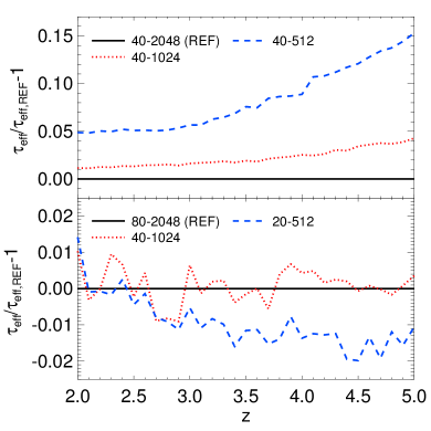
Figure 14: The redshift evolution of the effective optical depth relative to the reference model indicated in each panel. Top: Convergence with mass resolution for a fixed box size of $40h^{-1}\,\rm cMpc$. Bottom: Convergence with box size for a fixed mass resolution of $M_{\rm gas}=7.97\times 10^{5}h^{-1}\,M_{\odot}$. Note that $\tau_{\rm eff}$ has not been rescaled in this comparison.

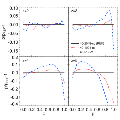
Figure 15: The probability distribution of the transmitted flux at $z=2,\,3,\,4$ and $5$ relative to the reference model indicated in the upper right panel. Each panel displays the convergence with mass resolution for a fixed box size of $40h^{-1}\,\rm cMpc$ at the four different redshifts. Note that $\tau_{\rm eff}$ has been rescaled to match Eq. (3) and the mock spectra are convolved with a $7\rm\,km\,s^{-1}$ Gaussian instrument profile.

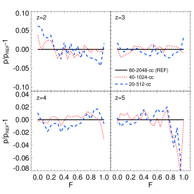
Figure 16: The probability distribution of the transmitted flux at $z=2,\,3,\,4$ and $5$ relative to the reference model indicated in the upper right panel. Each panel displays the convergence with box size for a fixed mass resolution of $M_{\rm gas}=7.97\times 10^{5}h^{-1}\,M_{\odot}$ at the four different redshifts. Note that $\tau_{\rm eff}$ has been rescaled to match Eq. (3) and the mock spectra are convolved with a $7\rm\,km\,s^{-1}$ Gaussian instrument profile.

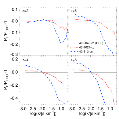
Figure 17: The power spectrum of the transmitted flux at $z=2,\,3,\,4$ and $5$ relative to the reference model indicated in the upper right panel. Each panel displays the convergence with mass resolution for a fixed box size of $40h^{-1}\,\rm cMpc$ at the four different redshifts. Note that $\tau_{\rm eff}$ has been rescaled to match Eq. (3) and the mock spectra are convolved with a $7\rm\,km\,s^{-1}$ Gaussian instrument profile for all models.

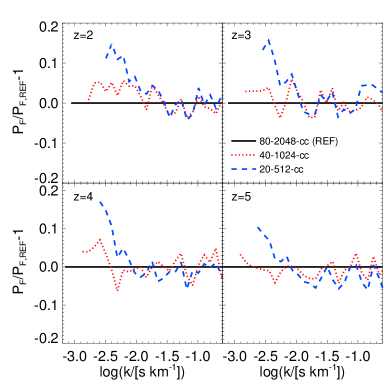
Figure 18: The power spectrum of the transmitted flux at $z=2,\,3,\,4$ and $5$ relative to the reference model indicated in the upper right panel. Each panel displays the convergence with box size for a fixed mass resolution of $M_{\rm gas}=7.97\times 10^{5}h^{-1}\,M_{\odot}$ at the four different redshifts. Note that $\tau_{\rm eff}$ has been rescaled to match Eq. (3) and the mock spectra are convolved with a $7\rm\,km\,s^{-1}$ Gaussian instrument profile.

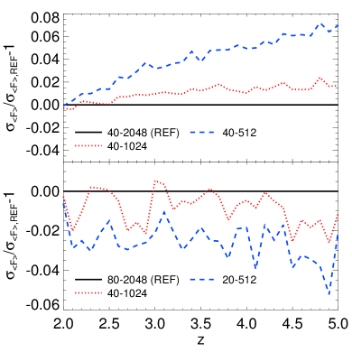
Figure 19: The redshift evolution of the standard deviation of the mean transmission in $3\rm\,pMpc$ segments relative to the reference model indicated in each panel. Top: Convergence with mass resolution for a fixed box size of $40h^{-1}\,\rm cMpc$. Bottom: Convergence with box size for a fixed mass resolution of $M_{\rm gas}=7.97\times 10^{5}h^{-1}\,M_{\odot}$. Note that $\tau_{\rm eff}$ has been rescaled to match Eq. (3).

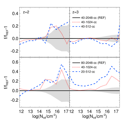
Figure 20: The column density distribution function at $z=2$ (left column) and $z=3$ (right column) relative to the reference models indicated in each row. Top panels: Convergence with mass resolution for a fixed box size of $40h^{-1}\,\rm cMpc$. Bottom panels: Convergence with box size for a fixed mass resolution of $M_{\rm gas}=7.97\times 10^{5}h^{-1}\,M_{\odot}$. Note that $\tau_{\rm eff}$ has been rescaled to match Eq. (3) for all models and the mock spectra have been processed as described in Section 2.2. The grey shading corresponds to the Poisson error in each bin.

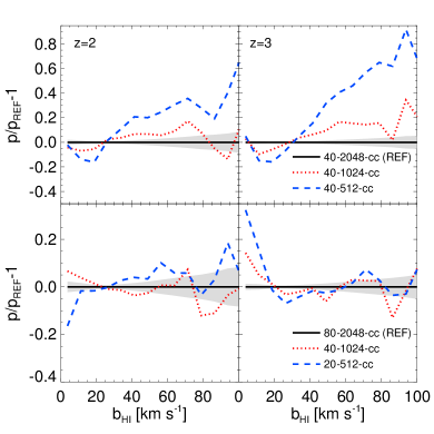
Figure 21: The velocity width distribution of Ly$\alpha$ absorption lines at $z=2$ (left column) and $z=3$ (right column) relative to the reference models indicated in each row. Top panels: Convergence with mass resolution for a fixed box size of $40h^{-1}\,\rm cMpc$. Bottom panels: Convergence with box size for a fixed mass resolution of $M_{\rm gas}=7.97\times 10^{5}h^{-1}\,M_{\odot}$. Note that $\tau_{\rm eff}$ has been rescaled to match Eq. (3) for all models and the mock spectra have been processed as described in Section 2.2. The grey shading corresponds to the Poisson error in each bin.

References

- Abel & Haehnelt (1999) Abel, T. & Haehnelt, M. G. 1999, ApJ, 520, L13
- Aldrovandi & Pequignot (1973) Aldrovandi, S. M. V. & Pequignot, D. 1973, A&A, 25, 137
- Altay et al. (2011) Altay, G., Theuns, T., Schaye, J., Crighton, N. H. M., & Dalla Vecchia, C. 2011, ApJ, 737, L37
- Arinyo-i-Prats et al. (2015) Arinyo-i-Prats, A., Miralda-Escudé, J., Viel, M., & Cen, R. 2015, J. Cosmology Astropart. Phys, 12, 017
- Bahcall & Peebles (1969) Bahcall, J. N. & Peebles, P. J. E. 1969, ApJ, 156, L7
- Becker & Bolton (2013) Becker, G. D. & Bolton, J. S. 2013, MNRAS, 436, 1023
- Becker et al. (2011) Becker, G. D., Bolton, J. S., Haehnelt, M. G., & Sargent, W. L. W. 2011, MNRAS, 410, 1096
- Becker et al. (2015) Becker, G. D., Bolton, J. S., Madau, P., Pettini, M., Ryan-Weber, E. V., & Venemans, B. P. 2015, MNRAS, 447, 3402
- Becker et al. (2013) Becker, G. D., Hewett, P. C., Worseck, G., & Prochaska, J. X. 2013, MNRAS, 430, 2067
- Bernardi et al. (2003) Bernardi, M. et al., 2003, AJ, 125, 32
- Bird et al. (2013) Bird, S., Vogelsberger, M., Sijacki, D., Zaldarriaga, M., Springel, V., & Hernquist, L. 2013, MNRAS, 429, 3341
- Bolton & Becker (2009) Bolton, J. S. & Becker, G. D. 2009, MNRAS, 398, L26
- Bolton et al. (2014) Bolton, J. S., Becker, G. D., Haehnelt, M. G., & Viel, M. 2014, MNRAS, 438, 2499
- Bolton et al. (2012) Bolton, J. S., Becker, G. D., Raskutti, S., Wyithe, J. S. B., Haehnelt, M. G., & Sargent, W. L. W. 2012, MNRAS, 419, 2880
- Bolton et al. (2005) Bolton, J. S., Haehnelt, M. G., Viel, M., & Springel, V. 2005, MNRAS, 357, 1178
- Bolton et al. (2008) Bolton, J. S., Viel, M., Kim, T.-S., Haehnelt, M. G., & Carswell, R. F. 2008, MNRAS, 386, 1131
- Borde et al. (2014) Borde, A., Palanque-Delabrouille, N., Rossi, G., Viel, M., Bolton, J. S., Yèche, C., LeGoff, J.-M., & Rich, J. 2014, J. Cosmology Astropart. Phys, 7, 005
- Bryan et al. (1999) Bryan, G. L., Machacek, M., Anninos, P., & Norman, M. L. 1999, ApJ, 517, 13
- Busca et al. (2013) Busca, N. G. et al., 2013, A&A, 552, A96
- Calura et al. (2012) Calura, F., Tescari, E., D’Odorico, V., Viel, M., Cristiani, S., Kim, T.-S., & Bolton, J. S. 2012, MNRAS, 422, 3019
- Carswell & Webb (2014) Carswell, R. F. & Webb, J. K. 2014, VPFIT: Voigt profile fitting program, Astrophysics Source Code Library
- Cen (1992) Cen, R. 1992, ApJS, 78, 341
- Cen et al. (1994) Cen, R., Miralda-Escudé, J., Ostriker, J. P., & Rauch, M. 1994, ApJ, 437, L9
- Croft et al. (2002) Croft, R. A. C., Weinberg, D. H., Bolte, M., Burles, S., Hernquist, L., Katz, N., Kirkman, D., & Tytler, D. 2002, ApJ, 581, 20
- Croft et al. (1999) Croft, R. A. C., Weinberg, D. H., Pettini, M., Hernquist, L., & Katz, N. 1999, ApJ, 520, 1
- Davé et al. (1999) Davé, R., Hernquist, L., Katz, N., & Weinberg, D. H. 1999, ApJ, 511, 521
- Dekker et al. (2000) Dekker, H., D’Odorico, S., Kaufer, A., Delabre, B., & Kotzlowski, H. 2000, in Proc. SPIE, Vol. 4008, Optical and IR Telescope Instrumentation and Detectors, ed. M. Iye & A. F. Moorwood, 534–545
- Fan et al. (2006) Fan, X. et al., 2006, AJ, 132, 117
- Faucher-Giguère et al. (2008a) Faucher-Giguère, C.-A., Lidz, A., Hernquist, L., & Zaldarriaga, M. 2008a, ApJ, 688, 85
- Faucher-Giguère et al. (2008b) Faucher-Giguère, C.-A., Prochaska, J. X., Lidz, A., Hernquist, L., & Zaldarriaga, M. 2008b, ApJ, 681, 831
- Finlator et al. (2012) Finlator, K., Oh, S. P., Özel, F., & Davé, R. 2012, MNRAS, 427, 2464
- Gnedin & Hui (1998) Gnedin, N. Y. & Hui, L. 1998, MNRAS, 296, 44
- Haardt & Madau (2012) Haardt, F. & Madau, P. 2012, ApJ, 746, 125
- Hernquist et al. (1996) Hernquist, L., Katz, N., Weinberg, D. H., & Miralda-Escudé, J. 1996, ApJ, 457, L51
- Hui & Gnedin (1997) Hui, L. & Gnedin, N. Y. 1997, MNRAS, 292, 27
- Katz et al. (1996) Katz, N., Weinberg, D. H., & Hernquist, L. 1996, ApJS, 105, 19
- Keating et al. (2016) Keating, L. C., Puchwein, E., Haehnelt, M. G., Bird, S., & Bolton, J. S. 2016, MNRAS, 461, 606
- Kim et al. (2007) Kim, T.-S., Bolton, J. S., Viel, M., Haehnelt, M. G., & Carswell, R. F. 2007, MNRAS, 382, 1657
- Kim et al. (2002) Kim, T.-S., Carswell, R. F., Cristiani, S., D’Odorico, S., & Giallongo, E. 2002, MNRAS, 335, 555
- Kim et al. (2013) Kim, T.-S., Partl, A. M., Carswell, R. F., & Müller, V. 2013, A&A, 552, A77
- Kim et al. (2004) Kim, T.-S., Viel, M., Haehnelt, M. G., Carswell, R. F., & Cristiani, S. 2004, MNRAS, 347, 355
- Kulkarni et al. (2015) Kulkarni, G., Hennawi, J. F., Oñorbe, J., Rorai, A., & Springel, V. 2015, ApJ, 812, 30
- Lamberts et al. (2015) Lamberts, A., Chang, P., Pfrommer, C., Puchwein, E., Broderick, A. E., & Shalaby, M. 2015, ApJ, 811, 19
- Lee (2012) Lee, K.-G. 2012, ApJ, 753, 136
- Lee et al. (2015) Lee, K.-G. et al., 2015, ApJ, 799, 196
- Lewis et al. (2000) Lewis, A., Challinor, A., & Lasenby, A. 2000, ApJ, 538, 473
- Lidz et al. (2010) Lidz, A., Faucher-Giguère, C.-A., Dall’Aglio, A., McQuinn, M., Fechner, C., Zaldarriaga, M., Hernquist, L., & Dutta, S. 2010, ApJ, 718, 199
- Lidz et al. (2006) Lidz, A., Heitmann, K., Hui, L., Habib, S., Rauch, M., & Sargent, W. L. W. 2006, ApJ, 638, 27
- Lukić et al. (2015) Lukić, Z., Stark, C. W., Nugent, P., White, M., Meiksin, A. A., & Almgren, A. 2015, MNRAS, 446, 3697
- McDonald (2003) McDonald, P. 2003, ApJ, 585, 34
- McDonald et al. (2001) McDonald, P., Miralda-Escudé, J., Rauch, M., Sargent, W. L. W., Barlow, T. A., & Cen, R. 2001, ApJ, 562, 52
- McDonald et al. (2000) McDonald, P., Miralda-Escudé, J., Rauch, M., Sargent, W. L. W., Barlow, T. A., Cen, R., & Ostriker, J. P. 2000, ApJ, 543, 1
- McDonald et al. (2006) McDonald, P. et al., 2006, ApJS, 163, 80
- McDonald et al. (2005) McDonald, P., Seljak, U., Cen, R., Bode, P., & Ostriker, J. P. 2005, MNRAS, 360, 1471
- McQuinn (2015) McQuinn, M. 2015, ARA&A in press, arXiv:1512.00086
- McQuinn et al. (2009) McQuinn, M., Lidz, A., Zaldarriaga, M., Hernquist, L., Hopkins, P. F., Dutta, S., & Faucher-Giguère, C.-A. 2009, ApJ, 694, 842
- McQuinn & Upton Sanderbeck (2016) McQuinn, M. & Upton Sanderbeck, P. R. 2016, MNRAS, 456, 47
- Meiksin et al. (2001) Meiksin, A., Bryan, G., & Machacek, M. 2001, MNRAS, 327, 296
- Meiksin & Tittley (2012) Meiksin, A. & Tittley, E. R. 2012, MNRAS, 423, 7
- Meiksin & White (2001) Meiksin, A. & White, M. 2001, MNRAS, 324, 141
- Meiksin & White (2003) Meiksin, A. & White, M. 2003, MNRAS, 342, 1205
- Meiksin (2009) Meiksin, A. A. 2009, Reviews of Modern Physics, 81, 1405
- Miralda-Escudé et al. (1996) Miralda-Escudé, J., Cen, R., Ostriker, J. P., & Rauch, M. 1996, ApJ, 471, 582
- Narayanan et al. (2000) Narayanan, V. K., Spergel, D. N., Davé, R., & Ma, C.-P. 2000, ApJ, 543, L103
- Nasir et al. (2016) Nasir, F., Bolton, J. S., & Becker, G. D. 2016, MNRAS in press, arXiv:1605.04155
- Palanque-Delabrouille et al. (2015) Palanque-Delabrouille, N. et al., 2015, J. Cosmology Astropart. Phys, 11, 011
- Palanque-Delabrouille et al. (2013) Palanque-Delabrouille, N. et al., 2013, A&A, 559, A85
- Pâris et al. (2011) Pâris, I. et al., 2011, A&A, 530, A50
- Pawlik et al. (2015) Pawlik, A. H., Schaye, J., & Dalla Vecchia, C. 2015, MNRAS, 451, 1586
- Pawlik et al. (2009) Pawlik, A. H., Schaye, J., & van Scherpenzeel, E. 2009, MNRAS, 394, 1812
- Planck Collaboration et al. (2014) Planck Collaboration et al. 2014, A&A, 571, A16
- Planck Collaboration et al. (2015) Planck Collaboration et al. 2015, A&A in press, arXiv:1502.01589
- Puchwein et al. (2015) Puchwein, E., Bolton, J. S., Haehnelt, M. G., Madau, P., Becker, G. D., & Haardt, F. 2015, MNRAS, 450, 4081
- Puchwein et al. (2012) Puchwein, E., Pfrommer, C., Springel, V., Broderick, A. E., & Chang, P. 2012, MNRAS, 423, 149
- Puchwein & Springel (2013) Puchwein, E. & Springel, V. 2013, MNRAS, 428, 2966
- Rahmati et al. (2013) Rahmati, A., Pawlik, A. H., Raicevic, M., & Schaye, J. 2013, MNRAS, 430, 2427
- Rauch (1998) Rauch, M. 1998, ARA&A, 36, 267
- Rauch et al. (1997) Rauch, M. et al., 1997, ApJ, 489, 7
- Regan et al. (2007) Regan, J. A., Haehnelt, M. G., & Viel, M. 2007, MNRAS, 374, 196
- Ricotti et al. (2000) Ricotti, M., Gnedin, N. Y., & Shull, J. M. 2000, ApJ, 534, 41
- Rollinde et al. (2013) Rollinde, E., Theuns, T., Schaye, J., Pâris, I., & Petitjean, P. 2013, MNRAS, 428, 540
- Rudie et al. (2012) Rudie, G. C., Steidel, C. C., & Pettini, M. 2012, ApJ, 757, L30
- Rudie et al. (2013) Rudie, G. C., Steidel, C. C., Shapley, A. E., & Pettini, M. 2013, ApJ, 769, 146
- Schaye et al. (2003) Schaye, J., Aguirre, A., Kim, T., Theuns, T., Rauch, M., & Sargent, W. L. W. 2003, ApJ, 596, 768
- Schaye et al. (2015) Schaye, J. et al., 2015, MNRAS, 446, 521
- Schaye et al. (1999) Schaye, J., Theuns, T., Leonard, A., & Efstathiou, G. 1999, MNRAS, 310, 57
- Schaye et al. (2000) Schaye, J., Theuns, T., Rauch, M., Efstathiou, G., & Sargent, W. L. W. 2000, MNRAS, 318, 817
- Seljak et al. (2006) Seljak, U., Makarov, A., McDonald, P., & Trac, H. 2006, Physical Review Letters, 97, 191303
- Slosar et al. (2013) Slosar, A. et al., 2013, J. Cosmology Astropart. Phys, 4, 026
- Springel (2005) Springel, V. 2005, MNRAS, 364, 1105
- Springel (2010) Springel, V. 2010, MNRAS, 401, 791
- Springel & Hernquist (2003) Springel, V. & Hernquist, L. 2003, MNRAS, 339, 289
- Springel et al. (2005) Springel, V. et al., 2005, Nature, 435, 629
- Tepper-García (2006) Tepper-García, T. 2006, MNRAS, 369, 2025
- Theuns et al. (1998) Theuns, T., Leonard, A., Efstathiou, G., Pearce, F. R., & Thomas, P. A. 1998, MNRAS, 301, 478
- Theuns et al. (2002) Theuns, T., Viel, M., Kay, S., Schaye, J., Carswell, R. F., & Tzanavaris, P. 2002, ApJ, 578, L5
- Tytler et al. (2009) Tytler, D., Paschos, P., Kirkman, D., Norman, M. L., & Jena, T. 2009, MNRAS, 393, 723
- Verner & Ferland (1996) Verner, D. A. & Ferland, G. J. 1996, ApJS, 103, 467
- Viel et al. (2013a) Viel, M., Becker, G. D., Bolton, J. S., & Haehnelt, M. G. 2013a, Phys. Rev. D, 88, 043502
- Viel et al. (2009) Viel, M., Bolton, J. S., & Haehnelt, M. G. 2009, MNRAS, 399, L39
- Viel et al. (2004a) Viel, M., Haehnelt, M. G., Carswell, R. F., & Kim, T.-S. 2004a, MNRAS, 349, L33
- Viel et al. (2004b) Viel, M., Haehnelt, M. G., & Springel, V. 2004b, MNRAS, 354, 684
- Viel et al. (2005) Viel, M., Lesgourgues, J., Haehnelt, M. G., Matarrese, S., & Riotto, A. 2005, Phys. Rev. D, 71, 063534
- Viel et al. (2013b) Viel, M., Schaye, J., & Booth, C. M. 2013b, MNRAS, 429, 1734
- Vogelsberger et al. (2014) Vogelsberger, M. et al., 2014, MNRAS, 444, 1518
- Vogt et al. (1994) Vogt, S. S. et al., 1994, in Proc. SPIE, Vol. 2198, Instrumentation in Astronomy VIII, ed. D. L. Crawford & E. R. Craine, 362
- Voronov (1997) Voronov, G. S. 1997, Atomic Data and Nuclear Data Tables, 65, 1
- Weymann (1966) Weymann, R. 1966, ApJ, 145, 560
- Worseck et al. (2014) Worseck, G. et al., 2014, MNRAS, 445, 1745
- Zhang et al. (1995) Zhang, Y., Anninos, P., & Norman, M. L. 1995, ApJ, 453, L57