Nonparametric hierarchical Bayesian quantiles

Abstract

Here we develop a method for performing nonparametric Bayesian inference on quantiles. Relying on geometric measure theory and employing a Hausdorff base measure, we are able to specify meaningful priors for the quantile while treating the distribution of the data otherwise nonparametrically. We further extend the method to a hierarchical model for quantiles of subpopulations, linking subgroups together solely through their quantiles. Our approach is computationally straightforward, allowing for censored and noisy data. We demonstrate the proposed methodology on simulated data and an applied problem from sports statistics, where it is observed to stabilize and improve inference and prediction.

Keywords: Censoring; Hausdorff measure, Hierarchical models; Nonparametrics; Quantile.

1 Introduction

Consider learning about $\beta$, the $\tau\in(0,1)$ quantile of the random variable $Z$. This will be based on data $\mathcal{D}=\{z_{1},...,z_{n}\}$, where we assume $z_{i}$, $i=1,2,...,n$, are scalars and initially that they are independent and identically distributed.  We will perform nonparametric Bayesian inference on $\beta$ given $\mathcal{D}$. The importance of quantiles is emphasized by, for example, Parzen (1979, 2004), Koenker and Bassett (1978) and Koenker (2005). By solving this problem we will also deliver a nonparametric Bayesian hierarchical quantile model, which allows us to analyze data with subpopulations only linked through quantiles. The methods extend to censored and partially observed data.

1.1 Background

In early work on Bayesian inference on quantiles, Section 4.4 of Jeffreys (1961) used a “substitute likelihood” $s(\beta)=\binom{n}{n_{\beta}}\tau^{n_{\beta}}(1-\tau)^{n-n_{\beta}}$, where $n_{\beta}=\sum_{i=1}^{N}1(z_{i}\leq\beta)$. See also Boos and Monahan (1986), Lavine (1995) and Dunson and Taylor (2005). This relates to other approximations to the likelihood suggested by Lazar (2003), Lancaster and Jun (2010) and Yang and He (2012), who use empirical likelihoods, and Chernozhukov and Hong (2003) who are inspired by some connections with M-estimators. Chamberlain and Imbens (2003) use a Bayesian bootstrap (Rubin (1981)) to carry out Bayesian inference on a quantile but have no control over the prior for $\beta$.

Yu and Moyeed (2001) carried out Bayesian analysis of quantiles using a likelihood based on an asymmetric Laplace distribution for the regression residuals $e_{i}=y_{i}-x_{i}^{\prime}\beta$ (see also Koenker and Machado (1999) and Tsionas (2003)), $L(\mathcal{D}|\beta)=\exp\{-\sum_{i=1}^{n}\rho_{\tau}(e_{i})\}$ where $\rho_{\tau}(\cdot)$ is the “check function” (Koenker and Bassett (1978)),

$$\rho_{\tau}(e)=|e|\left\{(1-\tau)1_{e<0}+\tau 1_{e\geq 0}\right\},\quad e\in R.$$ (1)

Here $\rho_{\tau}(e)$ is continuous everywhere, convex and differentiable at all points except when $e=0$. This Bayesian posterior is relatively easy to compute using mixture representations of Laplace distributions. Papers which extend this tradition include Kozumi and Kobayashi (2011), Li et al. (2010), Tsionas (2003), Kottas and Krnjajic (2009) and Yang et al. (2015). Unfortunately the Laplace distribution is a misspecified distribution and so typically yields inference which is overly optimistic. Yang et al. (2015) and Feng et al. (2015) discuss how to overcome some of these challenges, see the related works by Chernozhukov and Hong (2003) and Muller (2013).

Closer to our paper is Hjort and Petrone (2007) who assume the distribution function of $Z$ is a Dirichlet process with parameter $aF_{0}$, focusing on when $a\downarrow 0$. Hjort and Walker (2009) write down nonparametric Bayesian priors on the quantile function. Our focus is on using informative priors for $\beta$, but our focus on a non-informative prior for the distribution of $Z$ aligns with that of Hjort and Petrone (2007).

Our paper is related to Bornn et al. (2016) who develop a Bayesian nonparametric approach to moment based estimation. Their methods do not cover our case; the differences are brought out in the next section. The intellectual root is similar though: the quantile model only specifies a part of the distribution, so we complete the model by using Bayesian nonparametrics.

Hierarchical models date back to Stein (1966), while linear regression versions were developed by Lindley and Smith (1972). Discussions of the literature include Morris and Lysy (2012) and Efron (2010). Our focus is on developing models where the quantiles of individual subpopulations are thought of as drawn from a common population-wide mixing distribution, but where all other features of the subpopulations are nonparametric and uncommon across the populations. The mixing distribution is also nonparametrically specified. There is some linkages with deconvolution problems, see for example Butucea and Comte (2009) and Cavalier and Hengartner (2009), but our work is discrete and not linear. It is more related to, for example, Robbins (1956), Carlin and Louis (2008), McAuliffe et al. (2006) and Efron (2013) on empirical Bayes methods.

Here we report a simple to use method for handling this problem, which scales effectively with the sample size and the number of subpopulations. The method extends to allow for censored data. Our hierarchical method is illustrated on an example drawn from sports statistics.

1.2 Outline of the paper

In Section 2 we discuss our modelling framework and how we define Bayesian inference on quantiles. Particular focus is on uniqueness and priors. A flexible way of building tractable models is developed. This gives an analytic expression for the posterior on a quantile. A Monte Carlo analysis is carried out to study the bias, precision and coverage of our proposed method, which also compares the results to that seen for sample quantiles using central limit theories and bootstraps. In Section 3 we extend the analysis by introducing a nonparametric hierarchical quantile model and show how to handle it using very simple simulation methods. A detailed study is made of individual sporting careers using the hierarchical model, borrowing strengths across careers when the careers are short and data is limited. In Section 4 we extend the analysis to data which is censored and this is applied in practice to our sporting career example. Section 5 concludes, while an Appendix contains various proofs of results stated in the main body of the paper.

2 A Bayesian nonparametric quantile

2.1 Definition of the problem

We use the conventional modern definition of the $\tau$ quantile $\beta$, that is

$$\beta=\underset{b}{\mathop{\mathrm{a}rgmin}}\ \mathrm{E}\left\{\rho_{\tau}(Z-b)\right\}.$$

To start suppose $Z$ has known finite support $\mathcal{S}=\{s_{1},...,s_{J}\}$, and write

$$\Pr(Z=s_{j}|\theta)=\theta_{j},\quad\text{for }1\leq j\leq J,$$

with $\theta=(\theta_{1},\theta_{2},...,\theta_{J-1})^{\prime}\in\Theta_{\theta}$, and $\Theta_{\theta}\subseteq\Delta$, where $\Delta$ is the simplex, $\Delta=\{\theta;\ \iota^{\prime}\theta<1\text{ and }\theta_{j}>0\}$, and define $\theta_{J}=1-\iota^{\prime}\theta$, in which $\iota$ is a vector of ones. The function

$$\Psi(b,\theta)=\mathrm{E}_{\theta}\left\{\rho_{\tau}(Z-b)\right\}=\sum_{j=1}^{J}\theta_{j}\rho_{\tau}(s_{j}-b),$$

is continuous everywhere, convex and differentiable at all points except when $b\in\mathcal{S}$.

We define the “Bayesian nonparametric quantile” problem as learning from data the unknowns

$$(\beta,\theta^{\prime})^{\prime}\in\Theta_{\beta,\theta},\quad\text{where}\quad\Theta_{\beta,\theta}\subseteq\mathbb{R}\times\Delta\subset\mathbb{R}^{J}.$$

Each point within $\Theta_{\beta,\theta}$ is a pair $(\beta,\theta)$ which satisfies both the probability axioms and

$$\beta=\underset{b}{\mathop{\mathrm{a}rgmin}}\ \sum_{j=1}^{J}\theta_{j}\rho_{\tau}(s_{j}-b).$$

Here $\theta$ almost surely determines $\beta$ — this will be formalized in Proposition 1.

Unique $\beta$

(with probability $1$)

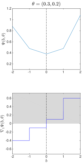
Non-unique $\beta$

(with probability $0$)

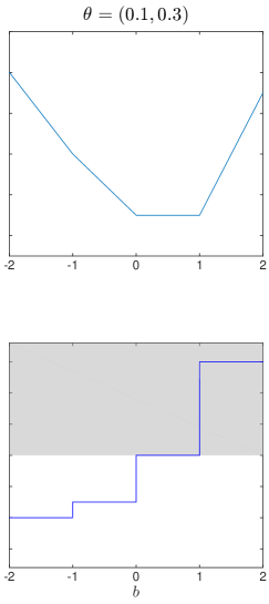
Figure 1: This plot shows the 0.4-quantile with support $S=\{-1,0,1\}$. Plotted is $\Psi(b,\theta)$ and its directional derivatives with respect to $b$, $\nabla_{1}\Psi(b,\theta)$. Left hand has $\theta=(0.3,0.2)^{\prime}$, the center is $\theta=(0.1,0.1)^{\prime}$,  and the right hand is $\theta=(0.1,0.3)^{\prime}$. In the left and center, the quantiles are are $0$ and $1$, respectively, while, in the right the optimization does not have a unique solution.  

Example 1

Figure 1 sets $\tau=0.4$, and $\mathcal{S}=\{-1,0,1\}$. In the left panel, for $\theta=(0.3,0.2)^{\prime}$, we plot $\Psi(b,\theta)$ and its directional derivatives with respect to $b$, $\nabla_{1}\Psi(b,\theta)$. The resulting quantile is $\beta=0$. In the center panels, $\theta=(0.1,0.1)^{\prime}$, implying $\beta=1$.  $\beta$ is not unique iff $\theta_{1}=0.4$ or $\theta_{1}+\theta_{2}=0.4$ — which are 0 probability events. An example of the latter case is $\theta=\left(0.1,0.3\right)^{\prime}$, which is shown in the right panel . Here $\Psi(b,\theta)$ is minimized on $[0,1]$.

Proposition 1 formalizes the connection between $\beta$ and $\theta$.

Proposition 1

Without loss of generality, assume $s_{1}<\cdots<s_{J}$. Then $\beta$ is unique iff $\tau\notin\{\theta_{1},\theta_{1}+\theta_{2},....,\theta_{1}+\cdots+\theta_{J-1}\}$. If $\theta$ has a continuous distribution with respect to the Lebesgue measure, then with probability 1, for each $\theta$ there is a unique quantile $\beta\in\mathcal{S}$ and with probability 1

$$\frac{\partial\beta}{\partial\theta^{\prime}}=0.\newline$$ (2)

Proposition 1 means we can partition the simplex in $J+1$ sets, $\Delta=\left(\bigcup_{k=1}^{J}\mathcal{A}_{k}\right)\cup\mathcal{N}$, where $\mathcal{N}$ is a zero Lebesgue measure set and the sets $\mathcal{A}_{k}=\{\theta\in\Delta;\ s_{k}=\underset{b}{\mathop{\mathrm{a}rgmin}}\ \Psi(b,\theta)\}$, $1\leq k\leq J$, contain all the values of $\theta$ which deliver a quantile $\beta=s_{k}=\underset{b}{\mathop{\mathrm{a}rgmin}}\ \Psi(b,\theta)$. We write this compactly as $\beta=t(\theta)$, $\beta\in\mathcal{S}$, $\theta\in\Delta$, and the corresponding set index $k=k(\theta)$, $1\leq k\leq J$, $\theta\in\Delta$, so $\beta=s_{k(\theta)}$.

Example 2 (continues=exa:QEExample1)

Figure 2 is a ternary plot showing all possible values of $\theta=\left(\theta_{1},\theta_{2}\right)^{\prime}$ and $\theta_{3}=1-\theta_{1}-\theta_{2}$ and the implied value of $\beta$ overlaid for $\tau=0.4$.  The values of $\theta$ which contain distinct values of $\beta$ are collected into the sets $\mathcal{A}_{1}$ (where $\beta=s_{1}$), $\mathcal{A}_{2}$ (where $\beta=s_{2}$), $\mathcal{A}_{3}$ (where $\beta=s_{3}$). The interior lines marking the boundaries between these sets are the zero measure events collected into $\mathcal{N}$. The union of the disjoint sets $\mathcal{A}_{1},\mathcal{A}_{2},\mathcal{A}_{3}$, and $\mathcal{N}$, make up the simplex $\Delta$.

Figure 2: Ternary plots of $\theta_{1},\theta_{2}$ and $\theta_{3}=1-\theta_{1}-\theta_{2}$ and the implied quantiles $\beta$ at level $\tau=0.4$.  Here $\beta\in\left\{s_{1},s_{2},s_{3}\right\}$. $\mathcal{A}_{k}$ is the set of probabilities $\theta_{1},\theta_{2}$ where $\beta=s_{k}$.

2.2 The prior and posterior

The set of admissible pairs $(\beta,\theta)$ is denoted by $\Theta_{\beta,\theta}\subseteq\mathcal{S}\times\Delta$. Now $\Theta_{\beta,\theta}$ is a lower dimensional space as $\beta=t(\theta)$. Using the Hausdorff measure, we are able to assign measures to the lower dimensional subsets of $\mathcal{S}\times\Delta$, and therefore we can define probability density functions with respect to Hausdorff measure on manifolds within $\mathcal{S}\times\Delta$.

One approach to building a joint prior $p(\beta,\theta)$ is to place a prior on $\beta\in\mathcal{S}$, which we write as

$$p(\beta),\quad\beta\in\mathcal{S}$$

and then build a conditional prior density,

$$p(\theta|\beta=s_{k}),\quad\theta\in\mathcal{A}_{k}$$

recalling $\mathcal{A}_{k}\subseteq\Delta$. Then the joint density with respect to Hausdorff measure on $\Theta_{\beta,\theta}$ is

$$p(\beta,\theta)=p(\beta)p(\theta|\beta).$$

For the quantile problem, with probability one $\beta=t(\theta)$, so the “area formula” of Federer (1969) (see also Diaconis et al. (2013) and Bornn et al. (2016)) implies the marginal density for the probabilities is induced as

$$p(\theta)=p(\beta,\theta),\quad\beta=t(\theta),$$

as Proposition 1 shows that $\partial\beta/\partial\theta^{\prime}=0$. Here the right hand side is the density of the prior with respect to Hausdorff measure defined on $\Theta_{\beta,\theta}$, while the left hand side is the implied density of the prior distribution of $\theta$ with respect to Lebesgue measure defined on the simplex $\Delta$.

The model’s likelihood is,

$$\prod_{j=1}^{J}\theta_{j}^{n_{j}},$$

where $n_{j}=\sum_{i=1}^{n}1(z_{i}=s_{j})$. Then the posterior distribution of $\beta,\theta$ will be,

$$p(\theta|\mathcal{D})=p(\beta=s_{k(\theta)},\theta|\mathcal{D})\propto p(\beta=s_{k(\theta)})p(\theta|\beta=s_{k(\theta)})\prod_{j=1}^{J}\theta_{j}^{n_{j}},\quad\beta=t(\theta).$$ (3)

This means that

$$p(\beta=s_{k}|\mathcal{D})=\int_{\mathcal{A}_{k}}p(\theta|\mathcal{D})\mathrm{d}\theta\propto p(\beta=s_{k})\int_{\mathcal{A}_{k}}\left\{p(\theta|\beta=s_{k})\prod_{j=1}^{J}\theta_{j}^{n_{j}}\right\}\mathrm{d}\theta.$$

2.3 A class of $p(\theta|\beta)$ models

Assume $f_{\Delta}(\theta)$ is the density function of a continuous distribution on $\Delta$, and define,

$$c_{k}=\Pr_{f_{\Delta}}(\beta=s_{k})=\int_{\mathcal{A}_{k}}f_{\Delta}(\theta)\mathrm{d}\theta.$$

Then one way to build an explicit prior for $p(\theta|\beta)$ is to decide to set

$$p(\theta|\beta=s_{k})=\frac{f_{\Delta}(\theta)}{c_{k}}1_{\mathcal{A}_{k}}(\theta),\quad\theta\in\mathcal{A}_{k}.$$

Proposition 2 shows how to compute $\left\{c_{k}\right\}$.

Proposition 2

Here $c_{1}=1-\Pr(\theta_{1}<\tau)$, $c_{J}=\Pr\left(\sum_{j=1}\theta_{j}<\tau\right)$, and $c_{k}=\Pr\left(\sum_{j=1}^{k-1}\theta_{j}<\tau\right)-\Pr\left(\sum_{j=1}^{k}\theta_{j}<\tau\right)$, for $k=2,...,J-1$.

This conditional distribution can be combined with a fully flexible prior $\Pr(\beta=s_{k})=b_{k}$, where $b_{k}>0$, for $1\leq k\leq J$, and $\sum_{k=1}^{J}b_{k}=1$. Returning to the general case, this implies the joint

$$p(\theta)=p(\beta=s_{k(\theta)},\theta)=\frac{b_{k(\theta)}}{c_{k(\theta)}}f_{\Delta}(\theta),$$ (4)

which in turn means, $\Pr(\beta=s_{k})=\int_{\mathcal{A}_{k}}p(\beta,\theta;\alpha)\mathrm{d}\theta=b_{k}$, the scientific marginal for $\beta$. Note that $p(\theta)$ is discontinuous at the set boundaries (that is the zero Lebesgue measure set $\mathcal{N}$), and $p(\theta)\neq f_{\Delta}(\theta)$ unless $b_{k}=c_{k}$ for all $k$.

From (3) the posterior distribution of $\beta,\theta$ will be,

$$p(\beta=s_{k(\theta)},\theta|\mathcal{D})\propto\frac{b_{k(\theta)}}{c_{k(\theta)}}f_{\Delta}(\theta)\prod_{j=1}^{J}\theta_{j}^{n_{j}},\quad\text{and\quad}p(\beta=s_{k}|\mathcal{D})\propto\frac{b_{k}}{c_{k}}\int_{\mathcal{A}_{k}}\left\{f_{\Delta}(\theta)\prod_{j=1}^{J}\theta_{j}^{n_{j}}\right\}\mathrm{d}\theta.$$

The Dirichlet case is particularly convenient.

2.4 Dirichlet special case

Let $f_{\Delta}$ be the Dirichlet density, $f_{D}(\theta;\alpha)=B(\alpha)^{-1}\prod_{j=1}^{J}\theta_{j}^{\alpha_{j}-1}$, where $\alpha=(\alpha_{1},...,\alpha_{J})$ is the vector of positive parameters, and $B(\alpha)$ is the beta function. Then $c_{k}$ can be computed via Proposition 2 using the distribution function of

$$\theta_{k}^{+}\sim Be\left(\alpha_{k}^{+},\alpha_{J}^{+}-\alpha_{k}^{+}\right),\quad\text{where generically\quad}\alpha_{k}^{+}=\sum_{j=1}^{k}\alpha_{j}.$$

To mark their dependence on $\alpha$, in the Dirichlet case we write $c_{k}=c_{k}(\alpha)$. We will refer to

$$p(\theta|\beta=s_{k})=\frac{f_{D}(\theta;\alpha)}{c_{k}}1_{\mathcal{A}_{k}}(\theta),\quad\theta\in\mathcal{A}_{k},$$ (5)

as the density function of $D_{J}(\alpha,k)$, the Dirichlet distribution truncated to $\mathcal{A}_{k}$.

This result can be used to power the following simple prior to posterior calculation.

Proposition 3

When $f_{\Delta}(\theta)=f_{D}(\theta;\alpha)$, then

$$\Pr(\beta=s_{k}|\mathcal{D})=\frac{1}{C(\alpha,\mathbf{n})}\frac{c_{k}(\alpha+\mathbf{n})}{c_{k}(\alpha)}\Pr(\beta=s_{k}),$$

where $\mathbf{n}=(n_{1},...,n_{J})$. Here $C(\alpha,\mathbf{n})$ is the normalizing constant, which is computed via enumeration, $C(\alpha,\mathbf{n})=\sum_{k=1}^{J}\frac{c_{k}(\alpha+\mathbf{n})}{c_{k}(\alpha)}b_{k}$. Further,

$$p(\theta|\mathcal{D})=\frac{1}{C(\alpha,\mathbf{n})}\frac{\Pr(\beta=s_{k(\theta)})}{c_{k(\theta)}(\alpha)}f_{D}(\theta;\alpha+\mathbf{n}).$$

The Bayesian posterior mean or quantiles of the posterior can be computed by enumeration unless $J$ is massive, in which case simulation can be used.

Discrete prior for median

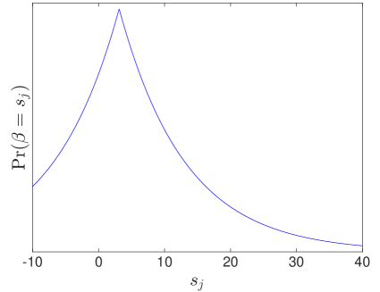
Posterior for median

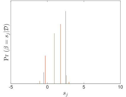
Figure 3: The left hand side shows the prior distribution of $\beta$ for the discrete method, and the right shows the corresponding posterior for the first replication. Notice the posterior has many small atoms marked in short green lines. These points originate from the prior and represent around $1$ data points.

2.5 Monte Carlo experiment   

Here $\mathcal{D}$ is simulated from the long right hand tailed $z_{i}\overset{iid}{\sim}-\log\chi_{1}^{2}$, so the $\tau$-quantile is $\beta_{\tau}=-\log\left\{F_{\chi_{1}^{2}}^{-1}(1-\tau)\right\}$. The empirical quantile $\widehat{\beta}_{\tau}$ will be used to benchmark the Bayesian procedures. The distribution of $\widehat{\beta}_{\tau}$ will be computed using its limiting distribution $\sqrt{n}\left(\widehat{\beta}_{\tau}-\beta_{\tau}\right)\overset{d}{\rightarrow}N(0,\tau(1-\tau)/f_{z}(\beta_{\tau})^{2})$ and by bootstrapping. In the case of the limiting distribution, the $f_{z}(\beta_{\tau})$ has been estimated by a kernel density estimator, with normal kernel and Silverman’s optimal bandwidth.

We build two Bayesian estimators:

1. Discrete.  The $s_{j}=-10+50(j-1)/(J-1)$, where $J=1,000$, and assume a weak prior for the median

   $$\Pr(\beta_{\tau}=s_{k})\propto\exp\left\{-\lambda\left|s_{k}-\delta_{\tau}\right|\right\},$$ (6)

   where $\lambda=0.1$, and $\delta_{\tau}=\beta_{\tau}+\gamma_{\tau}$, where $\gamma_{\tau}>0$, and we let $\gamma_{\tau}$ increases when $\tau$ deviates from $0.5$. This prior is not centered at the true value of the quantile and is more contaminated for the tail quantiles. In particular in our simulations we use $\gamma_{0.5}=2.333$ and $\gamma_{0.9}=6.032$. The data is binned using the support, and $\alpha=\frac{1}{J}$. The (6), for $\tau=0.5$, is shown in Figure 3 together with the associate posterior for one replication of simulated data.

2. Data.  The support $\mathcal{S}$ is the data (therefore $J=n$), $\alpha=\frac{1}{J}$, and the prior height (6) sits on those $J$ points of support (so the prior changes in each replication).

Table 1 reports

	$\tau=0.5$				$\tau=0.9$
	Sample quantile		Posterior		Sample quantile		Posterior
	CLT	Boot	Discrete	Data	CLT	Boot	Discrete	Data
	$n=10$
Bias	-0.157	0.152	0.345	0.206	1.245	-0.174	1.083	-0.167
$n^{1/2}$ SE	2.221	2.119	2.155	2.136	7.909	5.087	4.764	5.206
RMSE	0.720	0.687	0.764	0.706	2.794	1.618	1.856	1.655
Coverage	0.913	0.943	0.936	0.897	0.805	0.645	0.932	0.638
	$n=40$
Bias	-0.039	0.038	0.085	0.054	-0.224	0.050	0.438	0.098
$n^{1/2}$ SE	2.309	2.184	2.214	2.203	5.639	5.403	5.731	5.560
RMSE	0.367	0.347	0.360	0.353	0.919	0.856	1.007	0.885
Coverage	0.945	0.945	0.937	0.940	0.810	0.912	0.944	0.910
	$n=160$
Bias	0.020	0.010	0.021	0.014	0.072	0.014	0.102	0.025
$n^{1/2}$ SE	2.358	2.258	2.266	2.262	6.130	5.650	5.767	5.700
RMSE	0.187	0.179	0.180	0.179	0.490	0.447	0.467	0.451
Coverage	0.955	0.948	0.946	0.953	0.922	0.944	0.952	0.947
	$n=320$
Bias	-0.003	0.002	0.005	0.003	-0.015	0.002	0.023	0.004
$n^{1/2}$ SE	2.343	2.296	2.297	2.297	6.029	5.856	5.885	5.867
RMSE	0.093	0.091	0.091	0.091	0.239	0.231	0.234	0.232
Coverage	0.952	0.950	0.948	0.947	0.930	0.947	0.940	0.951

Table 1: Monte Carlo experiment using 25,000 replications and a highly biased prior. Coverage probability is based on a nominal 95% confidence or credible interval. Bayesian estimators are the posterior mean. RMSE denotes root mean square error. Boot denotes bootstrap, CLT implemented using a kernel for the asymptotic standard error.

the results from $25,000$ replications, comparing the five different modes of inference. It shows the asymptotic distribution of the empirical quantile provides a poor guide when working within a thin tail even when the $n$ is quite large. In the center of the distribution it is satisfactory by the time $n$ hits 40. The bootstrap performs poorly in the tail when $n$ is tiny, but is solid when $n$ is large.

Not surprisingly the bootstrap of the empirical quantile $\widehat{\beta}$ and the Bayesian method using support from the data are very similar. Assuming no ties, straightforward computations leads to,

$$\Pr(\widehat{\beta}=s_{j})=F_{\text{B}}\left(\lceil\tau J\rceil-1;J,(j-1)/J\right)-F_{\text{B}}\left(\lceil\tau J\rceil-1;J,j/J\right)$$

where $F_{\text{B}}(\cdot;n,p)$ is the binomial cumulative distribution function with size parameter $n$, and probability of success $p$. Interestingly, for large $J$, this is a close approximation to $c_{j}(\mathbf{1})$. This connection will become more explicit in the next subsection.

The discrete Bayesian procedure is by far the most reliable, performing quite well for all $n$. It does have a large bias for small $n$, caused by the poor prior, but the coverage is encouraging.  Overall, there is some evidence that for small samples the Bayesian estimators perform well in moderate to large samples. The two Bayesian procedures have roughly the same properties.

2.6 Comparison with Jeffrey’s substitution likelihood

Some interesting connections can be established by thinking of $\alpha$ as being small.

Proposition 4

Conditioning on the data, if $\alpha_{k}\downarrow 0$, and $\frac{\alpha_{k}}{\alpha_{l}}\rightarrow 1$, then $c_{k}(\alpha)\rightarrow\frac{1}{J}$, and,

$$c_{k}(\alpha+\mathbf{n}) \rightarrow \sum_{j=n_{k-1}^{+}}^{n_{k}^{+}-1}f_{\text{B}}(j;n-1,\tau),\quad k=1,2,...,J,$$

where, for $k=0,1,...,n$, $f_{\text{B}}(k;n,p)=$ $\binom{n}{k}p^{k}(1-p)^{n-k}$, is the binomial probability mass function with the size parameter $n$, and the probability of success $p$, and $n_{0}^{+}=0$.

The reason why $n-1$, not $n$,appears in the limit of $c_{k}(\alpha+\mathbf{n})$ is that $\mathcal{S}$ only has $n$ elements so $j$ runs from $0$ to $n-1$. The proposition means that if there are no ties in the data and $\mathcal{D}=\mathcal{S}$, then

$$\begin{array}[]{lll}c_{k}(\alpha+\mathbf{n})&\rightarrow&f_{\text{{B}}}(k-1;J-1,\tau),\quad k=1,2,...,J,\\ \Pr(\beta=s_{k}|\mathcal{D})&\rightarrow&C(\mathbf{n})^{-1}f(k-1;J-1,\tau)\Pr(\beta=s_{k}).\end{array}\quad$$

Here $C(\mathbf{n})$ is the normalizing constant, computed via enumeration, $C(\mathbf{n})=\sum_{k=1}^{J}f(k-1;J-1,\tau)b_{k}$.

The result in Proposition 4 is close to, but different from, Jeffrey’s substitution likelihood $s(\beta)=f(k;J,\tau)$, for $s_{k}\leq\beta<s_{k+1}$ where $s_{0}=-\infty$ and $s_{J+1}=\infty$ (Jeffrey has $n+1$ categories to choose from, not $n$, as he allows data outside the supposed $\mathcal{S}$). $s(\beta)$ is a piecewise constant, non-integrable function (which means it needs proper priors to make sense) in $\beta\in R$, while for us $\beta\in\mathcal{S}$ (and the posterior is always proper).

2.7 Comparison with Bayesian bootstrap

The prior and posterior distribution of $\beta$ in the Bayesian bootstrap are $\Pr(\beta=s_{k})=c_{k}(\alpha)$ and $\Pr(\beta=s_{k}|\mathcal{D})=c_{k}(\alpha+\mathbf{n})$, respectively. Therefore, Proposition 3 demonstrates that the choice of $b_{k}=c_{k}(\alpha)$ delivers the Bayesian bootstrap (here the results are computed analytically rather than via simulation). If a Bayesian bootstrap was run, each draw would be weighed by $w_{k}=b_{k}/c_{k}(\alpha)$ to produce a Bayesian analysis using a proper prior; $w_{k}$ is the ratio of the priors and does not depend upon the data. Finally, Proposition 4 implies that as $\alpha\downarrow 0$, so $c_{k}(\alpha)\rightarrow J^{-1}$. This demonstrates that, in the Bayesian bootstrap, the implied prior of $\beta$ is the uniform discrete distribution on the support of the data. In many applications this is an inappropriate prior.

Remark 1

To simulate from

$$p(\theta|\mathcal{D})=\frac{1}{C(\alpha,\mathbf{n})}\frac{b_{k(\theta)}}{c_{k(\theta)}(\alpha)}f_{D}(\theta;\alpha+\mathbf{n}),\quad b_{k}=\Pr(\beta=s_{k}),$$

write $m_{k}=\frac{b_{k}}{c_{k}}/C(\alpha,\mathbf{n})$, $m_{k}^{\prime}=b_{k}/c_{k}$, $M=\max\left(m_{1},...,m_{J}\right)$ and $M^{\prime}=\max\left(m_{1}^{\prime},...,m_{J}^{\prime}\right)$. Now $p(\theta|\mathcal{D})\leq Mf_{D}(\theta;\alpha+\mathbf{n})$, for any $\theta$. We can sample from $p(\theta|\mathcal{D})$ by drawing from $\text{Dirichlet}(\alpha+\mathbf{n})$ and accepting with probability $m_{k(\theta)}/M=m_{k(\theta)}^{\prime}/M^{\prime}$. The overall acceptance rate is $1/M$. If the prior on $\beta$ is weakly informative then $m_{k}^{\prime}\simeq 1$ for each $k$, and so the acceptance rate $m_{k(\theta)}^{\prime}/M^{\prime}\simeq 1$.

2.8 A cheap approximation

If $J$ is large, $\alpha\downarrow 0$ and no ties, then a central limit theory for binomial random variables implies

$$\frac{1}{J}\log f_{\text{B}}(k-1;J-1,\tau)\simeq-\frac{\left(\frac{k-1}{J-1}-\tau\right)^{2}}{2\tau\left(1-\tau\right)},$$

which should be a good approximation unless $\tau$ is in the tails, or $J$ is small. So the resulting trivial approximations to the main posterior quantities are

$$\widehat{\mathrm{E}}\left(\beta|\mathcal{D}\right) = \sum_{j=1}^{J}w_{j}^{\ast}s_{j},\quad w_{k}^{\ast}=w_{k}b_{k}/\sum_{j=1}^{J}w_{j}b_{j},\quad w_{k}=\exp\left\{-\frac{J\left(\frac{k-1}{J-1}-\tau\right)^{2}}{2\tau\left(1-\tau\right)}\right\},$$

$$\widehat{\mathrm{Var}}\left(\beta|\mathcal{D}\right) = \sum_{j=1}^{J}w_{j}^{\ast}\left\{s_{j}-\widehat{\mathrm{E}}\left(\beta|\mathcal{D}\right)\right\}^{2},\quad\widehat{F}_{\beta|\mathcal{D}}(\beta)=\sum_{j=1}^{J}w_{j}^{\ast}1_{s_{j}\leq\beta}\text{.}$$

When the prior is flat, this is a kernel weighted average of the data where the weights are determined by the ordering of the data. So large weights are placed on data with ranks $\left(k-1\right)/\left(J-1\right)$ which are close to $\tau$. This is very close to the literature on kernel quantiles, e.g. Parzen (1979), Azzalini (1981), Yang (1985) and Sheather and Marron (1990).

3 Hierarchical quantile models

3.1 Model structure

Assume a population is indexed by $i=1,2,...,I$ subpopulations, and that our random variable $Z$ again has known discrete support, $\mathcal{S}=\{s_{1},...,s_{J}\}$.  Then we assume within the $i$-th subpopulation

$$\Pr(Z=s_{j}|\theta,i)=\theta_{j}^{(i)},$$ (7)

thus allowing the distribution to change across the subpopulations. Here $\theta^{(i)}=(\theta_{1}^{(i)},...,\theta_{J-1}^{(i)})$, $\theta_{J}^{(i)}=1-\iota^{\prime(i)}$, and $\theta=(\theta^{(1)},...,\theta^{(I)})$. We assume the data $\mathcal{D}=\left\{Z_{1},...,Z_{n}\right\}$ are conditionally independent draws from (7). We assume that each time we see datapoints we also see which subpopulation the datapoint comes from. The data from the $i$-th population will be written as $\mathcal{D}_{i}$.

For the $i$-th subpopulation, the Bayesian nonparametric $\tau$ quantile is defined as

$$\beta_{i}=\underset{b}{\mathop{\mathrm{a}rgmin}}\ \sum_{j=1}^{J}\theta_{j}^{(i)}\rho_{\tau}(s_{j}-b).$$

Collecting terms $\beta=\left(\beta_{1},\beta_{2},...,\beta_{I}\right)^{\prime}$, the crucial assumption in our model is that

$$f(\theta|\beta)=\mathop{\displaystyle\prod}\limits_{i=1}^{I}f(\theta^{(i)}|\beta_{i}).$$

This says the distributions across subpopulations are conditionally independent given the quantile. That is, the single quantiles are the only feature which is shared across subpopulations.

We assume $\beta_{i}\in\mathcal{S}$, and the $\left\{\beta_{i}\right\}$ are i.i.d. across $i$, but from the shared distribution $\Pr(\beta_{i}=s_{j}|i,\pi)=\pi_{j}$, $i=1,2,...,I$, where $\pi=(\pi_{1},...,\pi_{J-1})$, and $\pi_{J}=1-\iota^{\prime}\pi$. We write a prior on $\pi$ as $p(\pi)$. Then the prior on the hierarchical parameters is

$$f(\beta,\pi)=f(\pi)f(\beta|\pi)=f(\pi)\mathop{\displaystyle\prod}\limits_{i=1}^{I}f(\beta_{i}|\pi).$$

This structured distribution will allow us to pool quantile information across subpopulations.

Our task is to make inference on $\left(\beta_{1},\beta_{2},...,\beta_{I}\right)^{\prime}$ from $\mathcal{D}$. When taken together, we call this a “nonparametric hierarchical quantile model”. This can also be thought of as related to the Robbins (1956) empirical Bayes method, but here each step is nonparametric.

By Bayes theorem,

$$f(\beta,\pi|\mathcal{D})\propto f(\beta,\pi)f(\mathcal{D}|\beta,\pi).$$ (8)

We will access this joint density using simulation.

• Algorithm 1: $\beta,\pi|\mathcal{D}$ Gibbs sampler 

1. Sample from $\Pr(\beta|\mathcal{D},\pi)=\mathop{\displaystyle\prod}\limits_{i=1}^{I}\Pr(\beta_{i}|\mathcal{D}_{i},\pi)$.

2. Sample from $f(\pi|\mathcal{D},\beta)=f(\pi|\beta)$.

In the Dirichlet case, we can sample from $\Pr(\beta_{i}|\mathcal{D}_{i},\pi)$ using Proposition 3.  If $f(\pi)$ is Dirichlet, then $\pi|\beta=$Dirichlet$(\lambda+\nu)$, where $\nu=(\nu_{1},...,\nu_{J})$, in which $\nu_{j}=\sum_{i=1}^{I}1(\beta^{(i)}=s_{j})$.

3.2 Example: batting records in cricket

We illustrate the hierarchical model using a dataset of the number of runs (which is a non-negative integer) scored in each innings by the most recent (by debut) $I=300$ English test players.  “Tests” are international matches, typically played over 5 days. Here we look at only games involving the English national team. This team plays matches against Australia, Bangladesh, India, New Zealand, Pakistan, South Africa, Sri Lanka, West Indies and Zimbabwe. Batsmen can bat up to twice in each test, but some players fail to get to bat in an individual game due to the weather or due to the match situation. Some players are elite batsmen and score many runs, others specialize in other aspects of the game and have poor batting records without any runs.

The database starts on 14th December 1951 and ends on 22nd January 2016. Some of these players never bat, others have long careers, the largest of which we see in our database is 235 innings, covering well over 100 test matches. In test matches batsmen can continue their innings for potentially a very long time and so can accumulate very high scores. An inning can be left incomplete for a number of reasons, so the score is right-censored — such innings are marked as being “not out”. By the rules of cricket at least 9% of the data must be right-censored. The database is quite large, but has a simple structure. The statistical challenge is with the data. Batting records are full of heterogeneity, highly skewed, partially censored and heavy tailed data. It is a good test case for our methods.

Interesting academic papers on the statistics of batting includes Kimber and Hansford (1993), which is a sustained statistical analysis of estimating the average performance of batsmen just using their own scores. Elderton (1945) is a pioneering cricket statistics paper in the same spirit. More recent papers include Philipson and Boys (2015) and Brewer (2013).

Our initial aim will be to make inference on the $0.5$ quantile for each and every batsmen, even if they have never batted. To start we will ignore the “not out” indicator. The player-by-player empirical median ranges from $0$ and $46$, and is itself heavily negatively skewed.

$50$% quantile

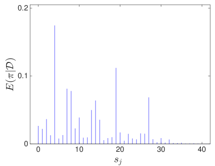
Posterior on median for $4$ players

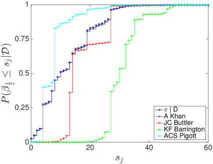
Figure 4: The left hand side shows the posterior distribution of the population probabilities of the quantiles $\pi_{j}=P(\beta=s_{j})$, $\tau=0.5$. The right hand side shows the posterior distribution of median of several players along with the posterior distribution of $\pi$. Notice in the case of Barrington there is only one innings which finished in the range 36 to 44 inclusive, which makes estimating the median unexpectedly hard (given how large a sample we have) and encourages the Bayesian method to aggressively shrink the estimator of the median.    

The common support of data for all the players is $\mathcal{S}=\{0,1,...,350\}$, therefore $J=351$. The prior distribution of $\theta^{(i)}$ is a Dirichlet distribution with $\alpha=(\alpha_{1},...,\alpha_{J})$, where $\alpha_{j}=4\tilde{\alpha}_{j}+\frac{1}{J}$ with $\tilde{\alpha}_{j}\propto e^{-0.03s_{j}}$ and $\sum_{j=1}^{J}\tilde{\alpha}_{j}=1$ (The empirical probability mass function of batting scores of all English players in the matches started between $1930$ and $1949$, $p_{i}=\Pr(Z=s_{j})$, is approximately proportional to $e^{-0.03s_{j}}$. Therefore our Dirichlet prior for $\theta$ is approximately centered around this empirical probability mass function with a large variability). We assume $\pi\sim\text{Dirichlet}(\lambda)$, where $\lambda_{j}=\tilde{\lambda}_{j}+\frac{1}{J}$, in which $\tilde{\lambda}_{j}\propto e^{-\frac{1}{2}\left(\frac{s_{j}-15}{15}\right)^{2}}$ for $j=1,...,J$, and $\sum_{j=1}^{J}\tilde{\lambda}_{j}=5$. In the left hand side of Figure 4 we have depicted $\mathrm{E}(\pi|\mathcal{D})$ for the $\tau=0.5$ median case. Figure 6 shows the results for the $\tau=0.3$ and $\tau=0.9$ cases. We will return to the non-median cases in the next subsection.

	Posterior						Posterior
Batsman	$\widetilde{\beta}_{1/2}$	Q5	Q95	$\widehat{\beta}_{1/2}$	$n_{i}$	Batsman	$\widetilde{\beta}_{1/2}$	Q5	Q95	$\widehat{\beta}_{1/2}$	$n_{i}$
A Khan	12.8	1	27	–	0	CJ Tavare	17.4	13	25	19.5	56
ACS Pigott	7.8	4	19	6	2	PCR Tufnell	1.2	0	2	1	59
A McGrath	13.1	4	27	34	5	MS Panesar	1.6	0	4	1	64
AJ Hollioake	4.9	2	12	3	6	CM Old	8.4	7	11	9	66
JB Mortimore	16.7	9	19	11.5	12	JA Snow	5.5	4	8	6	71
DS Steele	18.8	7	38	43	16	DW Randall	14.6	9	19	15	79
PJW Allott	6.6	4	14	6.5	18	RC Russell	14.6	10	20	15	86
JC Buttler	17.4	13	27	13.5	20	MR Ramprakash	18.7	14	21	19	92
W Larkins	12.8	7	25	11	25	PD Collingwood	23.2	19	28	25	115
NG Cowans	4.1	3	7	3	29	RGD Willis	4.1	4	5	5	128
JK Lever	5.4	4	10	6	31	KF Barrington	31	25	46	46	131
M Hendrick	3.4	1	4	2	35	APE Knott	17.6	13	24	19	149
DR Pringle	7.8	4	9	8	50	IT Botham	20.7	15	27	21	161
C White	11.5	7	19	10.5	50	DI Gower	26.9	25	28	27	204
GO Jones	15.9	10	22	14	53	AJ Stewart	25.6	19	28	27	235

Table 2:  Estimated median batting scores, treating not outs as if they were completed innings (i.e. ignoring right censoring). The batsman are ordered by sample size (i.e. the number of innings the batsman had). Table shows, for each batsmen, the mean of the Bayesian posterior of the median given the data, $\widetilde{\beta}_{1/2}$ = $E(\beta_{1/2}|\mathcal{D})$, the sample median $\widehat{\beta}_{1/2}$ and the sample size $n_{i}$. $Q_{5}$ and $Q_{95}$ are the estimates of the Bayesian 5% and 95% quantiles of the posterior distribution of the median, so indicates how uncertain we are about the Bayesian estimator of the mean. All the Bayesian quantities are estimated by simulation.

In the right hand side plot in Figure 4, the posterior distribution function of the median of scores for several players have been compared with the posterior distribution function of $\pi$ (the black curve). For the first player, A. Khan (the blue curve), no data are available as he never batted, and the distribution is indistinguishable from that for $\mathrm{E}(\pi|\mathcal{D)}$. A.C.S. Pigott played two innings for England, scoring 4 and 8 not out. The light blue curve shows that even with just two data points a lot of the posterior mass on the median has moved to the left, but the median is very imprecisely estimated (the estimate of median is $7.8$ with $95\%$ credible region $[4,19]$). The red curve corresponds to J. C. Buttler, whose sample median ($13$) is close to $\mathbb{E}_{\pi|\mathcal{D}}(\beta)=12.9$. His 20 actual scores were 85, 70, 45, 0, 59*, 13, 3*, 35*, 67, 14, 10, 73, 27, 7, 13, 11, 9, 12, 1, 42. His scores are not particularly heavy-tailed and so the median is reasonably well determined (the estimate of median is $17.4$ with $95\%$ credible region $[13,27]$). The green line shows the results for K. F. Barrington who batted 131 times and one of the highest averages of any English batsman. His median is relatively high ($31.0$) but surprisingly not well determined (with $95\%$ credible region $[25,46]$). Remarkably he has only once scored between 36 and 44 (inclusive), so there is a whole range of possible scores where there is no data. This stretches the Bayesian nonparametric interval. The right hand side of Figure 4 shows this clearly. Of course a 90% interval would be much shorter as it would not include this blank range.

Table 2 shows estimated posterior mean of the median for 30 players, together with sample sizes, 90% intervals, putting 5% of the posterior probability in each tail. Also given is the empirical median. The players are sorted by sample size. It shows that when the sample size is small there is a great deal of borrowing across the subpopulations. However, when the subpopulation is large then the hierarchy does not make much difference. McGrath’s scores are 69, 81, 34, 4, 13 (with sample median $34$), so he has very little data in the middle (he either fails or scores highly), and therefore the procedure shrinks the median a great deal towards a typical median result (the Bayesian estimate is $13.1$). Steele’s sample median ($43$) is very high (it is very similar to Barrington’s) and the sample size is low ($16$). The resulting Bayes estimate is still a high number ($18.8$), but is less than half of his sample median. Hence we think the evidence is that Steele was a very good batsmen, but there is not the evidence to rank him as a great batsman like Barrington. His record is more in line with Botham and Ramprakash.

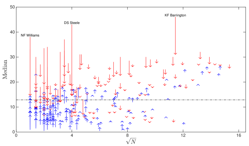
Figure 5: Sample median (arrow nocks) and mean of posterior distribution of medians (arrow heads) against the sample size for all players. The blue arrows indicate the estimates which were moved upwards, and the estimators which were moved down demonstrated by the red arrows. The dashed line is the expected value of $\beta$ under $E(\pi|D)$.

Figure 5 highlights the shrinkage of the sample median by the hierarchical model. We plot the batsman’s sample median $\widehat{\beta}_{1/2}$ against the batsman’s sample size $n_{i}$. Blue arrows show that the Bayesian posterior mean of the median is below the sample median, that is, it is shrunk down. Red arrows are the opposite, the Bayesian estimator is above the sample median, so is moved upwards. The picture shows there is typically more shrinkage for small sample sizes. But also, high sample medians are typically shrunk more than low sample medians, but there are more medians which are moved up than down. All this makes sense: the data are highly skewed, so high scores can occur due to high medians or by chance. Hence until we have seen a lot of high scores, we should shrink a high median down towards a more common value.

3.3 Estimating the quantile function

Of interest is $\beta_{\tau}$, the $\tau$-th quantile, as a function of $\tau$. Here we estimate that relationship pointwise, building a separate hierarchical model for each value of $\tau$. The only change we will employ is to set $\tilde{\lambda}_{j}\propto\exp\left\{-\left(s_{j}-\mu_{\tau}\right)^{2}/\sigma_{\tau}^{2}\right\}$, allowing $\mu_{\tau}=15+15\Phi^{-1}(\tau)$ and $\sigma_{\tau}=15$.

30% quantile

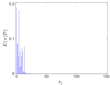
90% quantile

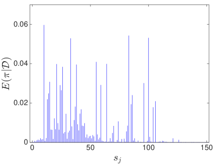
Figure 6: The left hand side shows the posterior distribution of the population probabilities of the quantiles $\pi_{j}=P(\beta=s_{j})$, $\tau=0.30$. The right hand side shows the corresponding result for $\tau=0.90$.

Figure 6 shows the common mixing distribution $\mathrm{E}\left(\pi|\mathcal{D}\right)$ for two quantile levels $\tau=0.30$ and $\tau=0.90$. Notice, of course, how different they are, with a great deal of mass on low scores when $\tau=0.30$ and vastly more scatter for $\tau=0.90$. This is because even the very best batsmen fail with a substantial probability, frequently recording very low scores. In the right hand tail, the difference between the skill levels of the players is much more stark, with enormous scatter.

We now turn to individual players. The dashed blue line in the left hand side of Figure 7 shows the empirical quantile function for P.J.W. Allott, while also plotted using a blue full line is the associated Bayesian quantile function $\mathrm{E}(\beta_{\tau}|\mathcal{D})$. The results are computed for $\tau\in\left\{0.01,0.2,...,0.99\right\}$. The Bayesian function also shows a central $90$% interval around the estimate.

The right hand side shows the same object but for K.F. Barrington, who tended to score very highly and also played a great deal (his $n_{i}$ is around 8 times larger than Allott’s). We can see in both players’ cases the lower quantiles are very precisely estimated and not very different, but at higher quantile levels the uncertainty is material and the differences in level stretch out. Further, at these higher levels the 90% intervals are typically skewed, with a longer right hand tail.

The Bayesian quantile functions seem shrunk more for Barrington, which looks odd as Allott has a smaller sample size. But Barrington has typically much higher scores (and so more variable) and so his quantiles are intrinsically harder to estimate and so are more strongly shrunk. His exceptionalism is reduced by the shrinkage.

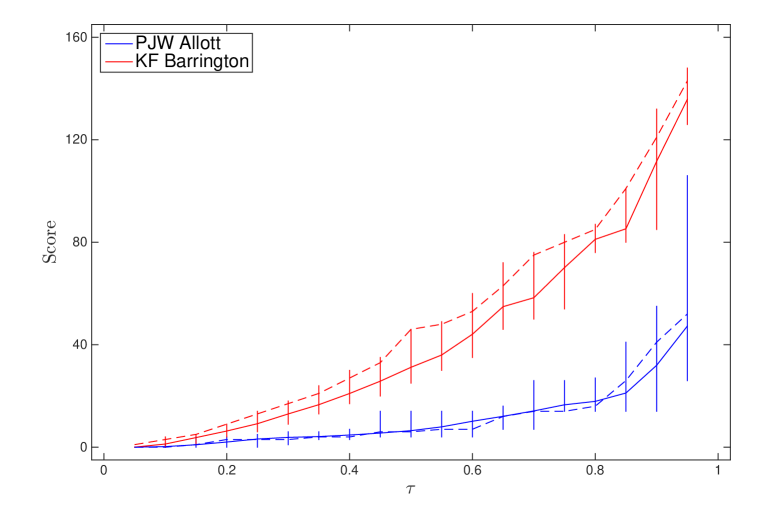
Figure 7: The pointwise estimated quantile function for two cricketers: P.J.W. Allott and K.F. Barrington. These calculations ignore the impact of censoring. Horizonal lines denote 90% posterior intervals with 5% in each tail. The curve for Allott uses his 18 innings, Barrington had 131 innings.  

For a moment we now leave the cricket example. We should note that we have ignored the fact some innings were not completed and marked “not out”, a form of censoring. We now develop methods to overcome this deficiency.

4 Truncated data

4.1 Censored data

Here we show how this methodology can be extended to models with truncated data. The probabilistic aspect of the model is unaltered. We assume the support is sorted and known to be $\mathcal{S}$, and $\Pr(Z=s_{j}|\theta)=\theta_{j}$.  However, in addition to some fully observed data, $\mathcal{D}_{1}=\{z_{1},...,z_{N}\}$, there exist $N^{\prime}$ additional data, $\mathcal{D}_{2}=\{s_{l_{i}},...,s_{l_{N^{\prime}}}\}$, which we know has been right truncated. We assume the non-truncated versions of the data are independent over $i$, such that $U_{i}\geq s_{l_{i}}$, $1\leq i\leq N^{\prime}$, $U_{i}\in\mathcal{S}$, $\Pr(U=s_{j}|\theta)=\theta_{j}$. We write $\mathcal{U=}\{U_{1},...,U_{N^{\prime}}\}$. Therefore our data is $\mathcal{D}=\mathcal{D}_{1}\bigcup\mathcal{D}_{2}$.

Inference on $(\beta,\pi)$ is carried out by augmenting it with $U$, and employing a Gibbs sampler in order to draw from $p(\beta,\pi,U|\mathcal{D})$.

4.2 Computational aspects

We implement this by Gibbs sampling, adding a first step to Algorithm 1.

• Algorithm 2: $\beta,\pi,U|\mathcal{D}$ Gibbs sampler 

1. Sample $\Pr(U|\beta,\mathcal{D},\pi).$

2. Sample $\Pr(\beta|\mathcal{D},U,\pi).$

3. Sample $f(\pi|\beta)$, returning to $1$.

Sampling from $U|\left(\beta=s_{k},\mathcal{D}\right)$ is not standard, but is also not difficult. We carry this out through data augmentation:

1. Sampling from $\Pr(U|\beta,\mathcal{D},\pi)$ by,

   1. Sample $\theta|\left(\beta=s_{k},\mathcal{D}\right)\mathcal{\sim}D_{J}(\alpha+\mathbf{n},k)$.

   2. Sample $U|\left(\beta=s_{k},\theta,\mathcal{D}\right)$.

Step 1(b) is straightforward, while 1(a) is a truncated Dirichlet defined in (5). The Appendix C shows how to simulate from $D_{J}(\alpha,k)$ exactly. As a side remark, it is tempting to sample $\theta|U,\mathcal{D}$ and $U|\theta,\mathcal{D}$ but this fails in practice; the reasons for this are described in detail in Appendix B.

4.3 A Bayesian bootstrap for the censored data

A Bayesian bootstrap algorithm can be developed to deal with the censored data (however its extension to hierarchical model is not straightforward, since priors on $\beta$ can not be incorporated in this algorithm). Independent draws from the Bayesian bootstrap posterior distribution can be obtained by the following algorithm.

• Algorithm 3: Bayesian bootstrap with censored data

1. Draw $\theta^{\ast}\sim\text{Dirichlet}(\alpha+\mathbf{n})$.

2. For $1\leq i\leq N^{\prime}$, draw $U_{i}$ from $\{s_{l_{i}},...,s_{J}\}$, with probability $\Pr(U_{i}=s_{j})=\frac{\theta_{j}^{\ast}}{\sum_{k=l_{i}}^{J}\theta_{k}^{\ast}}$, and set $n_{j}^{\prime}=\sum_{1}^{N^{\prime}}1(U_{i}=s_{j})$, and $\mathbf{n}^{\prime}=(n_{1}^{\prime},...,n_{J}^{\prime})$.

3. Draw $\theta\sim\text{Dirichlet}(\alpha+\mathbf{n}+\mathbf{n}^{\prime})$. Set $\beta=t(\theta)$. Go to $1$.

4.4 Returning to cricket: the impact of not outs

In cricket scores at least 9% of scores in each innings must be not out, so right censoring is important statistically. Not outs are particularly important for weaker batsmen who are often left not out at the end of the team’s innings. In Section 3.2 we ignored this feature of batting and here we return to it to correct the results.

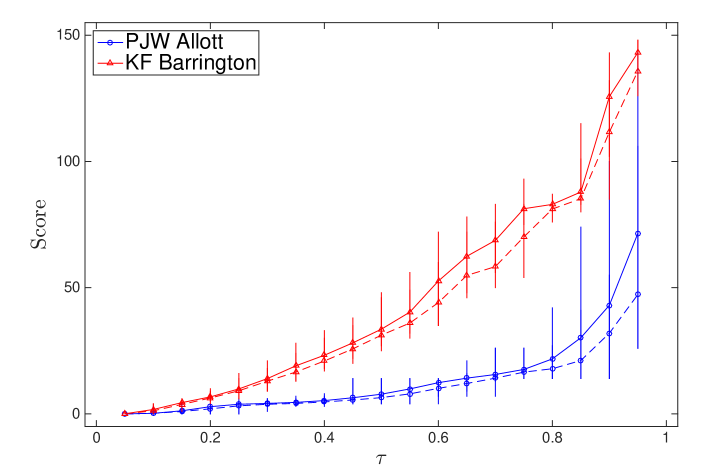
Figure 8: The censored-adjusted pointwise estimated quantile function for two cricketers: P.J.W. Allott and K.F. Barrington. The solid lines are the the estimates with the censored observations, and the dashed lines are obtained by ignoring that they are censored data. Horizonal lines denote 90% posterior intervals with 5% in each tail. The curve for Allott uses his 18 innings, Barrington had 131 innings.

Figure 8 shows the estimated pointwise quantile function for Barrington and Allott, taking into account the not outs.  Both are shifted upwards, particularly Allott in the right hand tail. However, Allott’s right hand tail is not precisely estimated.

				Ignoring censoring in analysis
	Bayesian			Bayesian			Empirical
Batsman	$\widetilde{\beta}_{1/2}$	$Q_{5}$	$Q_{95}$	$\widetilde{\beta}_{1/2}$	$Q_{5}$	$Q_{95}$	$n_{i}$	$n_{i}^{\prime}$	$\widehat{\beta}_{1/2}$
A Khan	14.7	4	30	12.7	2	27	0	0	–
ACS Pigott	9.7	4	27	7.8	4	19	2	1	4
A McGrath	14.3	4	31	13	4	27	5	0	34
AJ Hollioake	5.5	4	14	4.7	2	12	6	0	2
JB Mortimore	16.4	9	20	16.7	9	19	12	2	11
DS Steele	19.4	7	37	18.8	7	35	16	0	42
PJW Allott	7.8	4	14	6.7	4	14	18	3	6
JC Buttler	17.7	13	27	17.1	13	27	20	3	13
W Larkins	12.6	7	27	13.3	7	25	25	1	11
NG Cowans	5.9	4	10	4.1	3	7	29	7	3
JK Lever	6.7	4	11	5.3	4	8.5	31	5	6
M Hendrick	6.3	4	10	3.4	1	5	35	15	2
DR Pringle	8.3	7	10	7.7	4	9	50	4	8
C White	13.1	8	19	11.7	7	19	50	7	10
GO Jones	17.1	10	22	15.9	10	19	53	4	14
CJ Tavare	17.4	12.5	25	17.3	13	25	56	2	22
PCR Tufnell	4.8	1	9	1.2	0	2	59	29	1
MS Panesar	4	4	4	1.6	0	4	64	21	1
CM Old	8.9	7	13	8.4	7	11	66	9	9
JA Snow	7.9	4	9	5.5	4	8	71	14	6
DW Randall	14.6	9	19	14.5	10	19	79	5	15
RC Russell	16.2	9.5	24	14.6	12	20	86	16	15
MR Ramprakash	18.8	14	21	18.6	14	21	92	6	19
PD Collingwood	25	19	30	23.3	19	28	115	10	25
RGD Willis	8.5	7	10	4.1	4	5	128	55	5
KF Barrington	33.7	27	48	31	25	46	131	15	46
APE Knott	18.9	14	27	17.5	13	24	149	15	19
IT Botham	20.6	15	27	20.7	15	27	161	6	21
DI Gower	27.5	26	32	27	25	28	204	18	27
AJ Stewart	26.3	19	29.5	25.6	19	28	235	21	27

Table 3: Estimated median batting scores. Sample median is compared with two Bayesian estimators, where $\widetilde{\beta}_{1/2}$ = $E(\beta_{1/2}|D)$. $n_{i}$ is the number of innings, $n_{i}^{\prime}$ denotes the number of not outs which are treated as right censored data and $\widehat{\beta}_{1/2}$ is the empirical median. In the first model the not outs are assumed to be right censored observations. In the second model they are treated as if they were completed innings. $Q_{5}$ denotes the estimated 5% point on the relevant posterior distribution.

Table 3 shows the Bayesian results for our selected 30 players, updating Table 2 to reflect the role of right censoring. Here $n_{i}^{\prime}$ denotes the number of not out, that is right censored innings, the player had. In many cases this is between 10% and 20% of the innings, but for some players it is far higher. R.G.S. Willis is the leading example, who had 55 not outs of 128 innings. A leading bowler, he usually batted towards the end of innings and was often left not out. His posterior mean of the median is inflated greatly by the statistical treatment of censoring. Further, the interval between $Q_{5}$ and $Q_{95}$ is widened substantially. Other players are hardly affected, e.g. M.R. Ramprakash, who had 6 not outs in 92 innings.

Table 3 shows a ranking of players by the mean of the posteriors of the quantiles, at three different levels of quantiles. This shows how the rankings change greatly with the quantile level. For small levels, we can think of this as being about consistency. For the median it is about typical performance. For the 90% quantile this is about upside potential to bat long. A remarkable result is J.B. Bolus who has a very high $\beta_{0.30}$ quantile. His career innings were the following: 14, 43, 33, 15, 88, 22, 25, 57, 39, 35, 58, 67. He only played for a single year, but never really failed in a single inning. However he never managed to put together a very long memorable innings and this meant his Test career was cut short by the team selectors. They seem to not so highly value reliability.

	0.3 quantile				0.5 quantile				0.9 quantile
rank	Batsman	$\widetilde{\beta}_{0.3}$	Q5	Q95	Batsman	$\widetilde{\beta}_{0.5}$	Q5	Q95	Batsman	$\widetilde{\beta}_{0.9}$	Q5	Q95
1	JB Bolus	16.6	4	33	KF Barrington	33.7	27	48	KF Barrington	121.3	101	143
2	KF Barrington	14.0	9	21	KP Pietersen	30.5	26	34	IR Bell	116.8	109	121
3	DI Gower	13.1	11	16	JH Edrich	29.5	22	35	GP Thorpe	115.8	94	119
4	AN Cook	12.9	11	13	G Boycott	29.1	23	35	PH Parfitt	115.6	86	121
5	ER Dexter	12.8	10	16	ER Dexter	28.5	27	32	IJL Trott	111.2	64	121
6	G Boycott	12.6	10	13	ME Trescothick	28.4	24	32	MC Cowdrey	111.1	96	119
7	GA Gooch	12.6	10	13	BL D’Oliveira	28.2	23	32	G Boycott	109.7	106	116
8	KP Pietersen	12.6	9	14	AJ Strauss	28.1	25	32	DL Amiss	106.9	64	119
9	RW Barber	12.5	6	13	R Subba Row	27.9	22	32	AN Cook	106.7	96	118
10	AJ Strauss	12.5	9	14	DI Gower	27.5	26	32	MP Vaughan	106.3	100	115
11	G Pullar	12.4	9	14	MC Cowdrey	27.3	23	32	ME Trescothick	105.4	90	113
12	ME Trescothick	12.4	9	14	AW Greig	27.2	19	32	KP Pietersen	105.2	96	119
13	MP Vaughan	12.4	9	13	AN Cook	27.2	22	32	AJ Strauss	105.0	83	112
14	MC Cowdrey	12.3	9	13	GA Gooch	27.1	22	30	AW Greig	102.8	96	110
15	JE Root	12.2	6	13	JB Bolus	27.1	15	36	N Hussain	102.5	85	109
16	R Subba Row	12.1	8	13	GP Thorpe	27.1	19	32	CT Radley	102.4	59	106
17	RA Smith	12.1	8	13	IJL Trott	26.7	19	35	JE Root	102.1	83	130
18	JM Parks	12.0	7	14	AJ Stewart	26.3	19	29	DI Gower	101.8	85	106
19	JG Binks	12.0	6	13	PH Parfitt	25.8	18	32	AJ Lamb	101.4	83	119
20	GP Thorpe	11.8	9	13	MP Vaughan	25.7	19	32	DS Steele	100.8	64	106

Table 4: Best $20$ players ranked based on the mean of the posteriors of the quantiles, at three different levels of quantiles.

Again K.F. Barrington is the standout batsman. He is very strong at all the different quantiles. Notice though he still had a 30% chance of scoring 14 or less — which would be regarded by many cricket watchers as a failure. But once his innings was established his record was remarkably strong, typically playing long innings.

5 Conclusions

In this paper we provide a Bayesian analysis of quantiles by embedding the quantile problem in a larger inference challenge. This delivers quite simple ways of performing inference on a single quantile. The frequentist performance of our methods are similar to that of the bootstrap.

We extend the framework to introduce a hierarchical quantile model, where each subpopulation’s distribution is modeled nonparametrically but linked through a nonparametric mixing distribution placed on the quantile. This allows non-linear shrinkage, adjusting to skewed and sparse data in an automatic manner.

This approach is illustrated by the analysis of a large database from sports statistics of 300 Test cricketers. Each person’s batting performance is modeled nonparametrically and separately, but linked through a quantile which is drawn from a common distribution. This allows us to shrink each cricketer’s performance – a particular advantage in cases where the careers are very short.

The modeling approach is extended to allow for truncated data. This is implemented by using simulation based inference. Again this set is illustrated in practice by looking at not outs in batting innings, where we think of the data as right censored.

Appendix A Appendix

A.1 Proof or Proposition 1

As $\Psi(b,\theta)$ is a convex function it has a unique minimizer on $\mathbb{R}$, or its optimal set is a closed interval, $[\beta_{l},\beta_{u}]$, where $s_{1}\leq\beta_{l}<\beta_{u}\leq s_{J}$ (Rockafellar (1970)). In the latter case, there exist $\beta_{m}\in[\beta_{l},\beta_{u}]\backslash\mathcal{S}$, at which $\frac{\partial\Psi(b,\theta)}{\partial b}$ exists and is equal to zero,

$$\left.\frac{\partial\Psi(b,\theta)}{\partial b}\right|_{b=\beta_{m}}=(1-\tau)\tau^{\prime}-\tau(1-\tau^{\prime})=0$$

where $\tau^{\prime}=\sum_{j=1}^{k}\theta_{j}$, and $k=\max\{j;s_{j}<\beta_{m}\}$. For a specific value of $\beta_{m}$, this equality holds if $\tau^{\prime}=\tau$, that means, $\sum_{j=1}^{k}\theta_{j}=\tau$. This implies that the minimizer of $\Psi(b,\theta)$ is not unique if and only if $\tau\in\{\theta_{1},\theta_{1}+\theta_{2},....,\theta_{1}+\cdots+\theta_{J-1}\}$, and this is a zero measure event if $\theta$ is non-singular.

Now assume $\beta^{\ast}$ is the unique minimizer of $\Psi(b,\theta)$ for $\theta=\theta^{\ast}$. This implies that the directional derivatives of $\Psi(b,\theta)$ are strictly positive at the optimal point, $\nabla_{v}\Psi(\beta^{\ast},\theta^{\ast})>0$, for$\quad v\in\{-1,1\}$. However, $\nabla_{v}\Psi(\theta,b)$ is an affine (and therefore a continuous) function of $\theta$,

$$\nabla_{v}\Psi(b,\theta)=\sum_{j=1}^{J}(1-\tau)\theta_{j}v1(s_{j}<b)-\tau\theta_{j}v1(s_{j}>b)+\theta_{j}\rho_{\tau}(-v)1(s_{j}=b),$$

therefore there exists an open ball centered at $\theta^{\ast}$ with radius $\delta>0$, $\mathcal{B}_{\delta}(\theta^{\ast})$, in such a way that, $\forall v\in\{-1,1\}$, $\forall\theta\in\mathcal{B}_{\delta}(\theta^{\ast})$, $\nabla_{v}\Psi(\beta^{\ast},\theta)>0$. Hence, for any $\theta\in\mathcal{B}_{\delta}(\theta^{\ast})$, the objective function $\Psi(b,\theta)$ has a unique minimizer at $\beta^{\ast}$: $\forall\theta\in\mathcal{B}_{\delta}(\theta^{\ast})$, $\beta^{\ast}=\underset{b}{\mathop{\mathrm{a}rgmin}}\ \Psi(b,\theta)$, and this implies, $\left.\partial\beta/\partial\theta^{\prime}\right|_{\theta=\theta^{\ast}}=0$.

A.2 Proof of Proposition 2

For $k=1$, $\mathcal{A}_{1}=\{\theta;\theta_{1}>\tau\}$, therefore, $c_{1}=\Pr(\theta\in\mathcal{A}_{1})=\Pr(\theta_{1}>\tau)$. For $2\leq k\leq J-1$, we have,

$$\mathcal{A}_{k}=\left\{\theta;\sum_{j=1}^{k-1}\theta_{j}<\tau,\ \ \text{and}\ \ \sum_{j=1}^{k}\theta_{j}>\tau\right\}=\left\{\theta;\sum_{j=1}^{k-1}\theta_{j}<\tau\right\}\backslash\left\{\theta;\sum_{j=1}^{k}\theta_{j}\leq\tau\right\}.$$

Since $\left\{\theta;\sum_{j=1}^{k}\theta_{j}\leq\tau\right\}\subset\left\{\theta;\sum_{j=1}^{k-1}\theta_{j}<\tau\right\}$, then, $c_{k}=\Pr(\theta\in\mathcal{A}_{k})=\Pr\left(\sum_{j=1}^{k-1}\theta_{j}<\tau\right)-\Pr\left(\sum_{j=1}^{k}\theta_{j}<\tau\right)$. Finally, for $k=J$, $\mathcal{A}_{J}=\left\{\theta;\sum_{j=1}\theta_{j}<\tau\right\}$, and so $c_{J}=\Pr\left(\sum_{j=1}\theta_{j}<\tau\right)$.

A.3 Proof of Proposition 3

In the Dirichlet case the posterior distribution of $\beta,\theta$ will be,

$$p(\beta=s_{k(\theta)},\theta|\mathcal{D})\propto\left(\prod_{j=1}^{J}\theta_{j}^{n_{j}}\right)\frac{b_{k(\theta)}}{c_{k(\theta)}(\alpha)}f_{D}(\theta;\alpha)=\frac{1}{c(\alpha+n)}\frac{b_{k(\theta)}}{c_{k(\theta)}(\alpha)}f_{D}(\theta;\alpha+n),$$

where $n=(n_{1},...,n_{J})$ and $c(\alpha+n)=\int_{\Delta}f_{D}(\theta;\alpha+n)\mathrm{d}\theta$. The right hand side integrates to $C(\alpha,n)=\sum_{k=1}^{J}\frac{c_{k}(\alpha+n)}{c_{k}(\alpha)}b_{k}$, hence the normalized posterior is $p(\beta=s_{k(\theta)},\theta|\mathcal{D})=m_{k(\theta)}f_{D}(\theta;\alpha+n)$, where $m_{k}=\frac{1}{C(\alpha,n)}\frac{b_{k}}{c_{k}(\alpha)}$.

The posterior distribution of $\beta$ can be found analytically, recalling that for quantiles the area formula implies $p(\theta|\mathcal{D})=p(\beta,\theta|\mathcal{D})$, as $\Pr(\beta=s_{k}|\mathcal{D})=\int_{\mathcal{A}_{k}}p(\theta|\mathcal{D})\mathrm{d}\theta=\frac{1}{C(\alpha,n)}\frac{c_{k}(\alpha+n)}{c_{k}(\alpha)}b_{k}$.

A.4 Proof of Proposition 4

Note that,

$$\underset{\alpha,\beta\rightarrow 0}{\lim}B(\alpha,\beta) = \underset{\alpha,\beta\rightarrow 0}{\lim}\frac{\Gamma(\alpha)\Gamma(\beta)}{\Gamma(\alpha+\beta)}=\underset{\alpha,\beta\rightarrow 0}{\lim}\frac{\Gamma(\alpha+1)\Gamma(\beta+1)}{\Gamma(\alpha+\beta+1)}\frac{\alpha+\beta}{\alpha\beta}=\underset{\alpha,\beta\rightarrow 0}{\lim}\frac{\alpha+\beta}{\alpha\beta},$$

$$\underset{\alpha,\beta\rightarrow 0}{\lim}\alpha B(\tau;\alpha,\beta) = \underset{\alpha,\beta\rightarrow 0}{\lim}\alpha\frac{\tau^{\alpha}(1-\tau)^{\beta}}{\alpha}\left(1+\frac{\alpha+\beta}{\alpha+1}\tau+\frac{(\alpha+\beta)(\alpha+\beta+1)}{(\alpha+1)(\alpha+2)}\tau^{2}+\cdots\right)=1.$$

Hence, $\underset{\alpha,\beta\rightarrow 0}{\lim}I_{\tau}(\alpha,\beta)=\beta/\left(\alpha+\beta\right)$. Assume all the elements of $\alpha$ goes to $0$ at the same rate,

$$c_{k}(\alpha) \rightarrow \underset{\alpha_{k}\downarrow 0}{\lim}\ I_{\tau}(\alpha_{k-1}^{+},\alpha_{J}^{+}-\alpha_{k-1}^{+})-I_{\tau}(\alpha_{k}^{+},\alpha_{J}^{+}-\alpha_{k}^{+})$$

$$\rightarrow \underset{\varepsilon\downarrow 0}{\lim}\ I_{\tau}((k-1)\varepsilon,(J-k+1)\varepsilon)-I_{\tau}(k\varepsilon,(J-k)\varepsilon)=\frac{J-k+1}{J}-\frac{J-k}{J}=\frac{1}{J}.$$

As $\alpha\downarrow 0$, so $\theta_{k}^{+}\overset{L}{\rightarrow}\text{Beta}(n_{k}^{+},n-n_{k}^{+})$. Now using that limit, $\Pr(\theta_{k}^{+}<\tau)=I_{\tau}(n_{k}^{+},n-n_{k}^{+})$. For $\tau\in(0,1)$, and positive integers $k$ and $n$, $I_{\tau}(k,n)=1-F_{\text{B}}(k-1;n+k-1,\tau)$. So, for $2\leq k\leq J-1$,

$$c_{k} = \Pr(\theta_{k-1}^{+}<\tau)-\Pr(\theta_{k}^{+}<\tau)=I_{\tau}(n_{k-1}^{+},n-n_{k-1}^{+})-I_{\tau}(n_{k}^{+},n-n_{k}^{+})$$

$$= F_{\text{B}}(n_{k}^{+}-1;n-1,\tau)-F_{\text{B}}(n_{k-1}^{+}-1;n-1,\tau)=\sum_{k=n_{k-1}^{+}}^{n_{k}^{+}-1}f_{\text{B}}(k;n-1,\tau),$$

$$c_{1} = 1-\Pr(\theta_{1}^{+}<\tau)=F_{\text{B}}(n_{1}^{+}-1;n-1,\tau)=\sum_{k=0}^{n_{1}^{+}-1}f_{\text{B}}(k;n-1,\tau)=\sum_{k=n_{0}^{+}}^{n_{1}^{+}-1}f_{\text{B}}(k;n-1,\tau)$$

$$c_{J} = \Pr(\theta_{J-1}^{+}<\tau)=1-F_{\text{B}}(n_{J-1}^{+}-1;n-1,\tau)=\sum_{k=n_{J-1}^{+}}^{n-1}f_{\text{B}}(k;n-1,\tau)=\sum_{k=n_{J-1}^{+}}^{n_{J}^{+}-1}f_{\text{B}}(k;n-1,\tau),$$

where $n_{0}^{+}=0$. If there are no ties, n=J, and $z_{1}=s_{1}<\cdots<z_{J}=s_{J}$, then the result holds.

Appendix B A basic simulator which does not work

The $U=(U_{1},...,U_{N^{{}^{\prime}}})$, will be treated as missing data, and the inference can be performed by sampling from $\pi,\theta,U|\mathcal{D}$. To do this we would need to sample from $p(\theta,U|\mathcal{D})$.

One approach to sampling from this is using a Gibbs sampler.

• Algorithm 2: $\theta,U|\mathcal{D}$ Gibbs sampler

1. Draw from, $\theta|\mathcal{D},U\sim$Dirichlet$(\alpha+\mathbf{n}+\mathbf{n}^{\prime})$, $\mathbf{n}^{\prime}=(n_{1}^{\prime},...,n_{J}^{\prime})$, $n_{j}^{{}^{\prime}}=\sum_{i=1}^{N^{\prime}}1(U_{i}=s_{j})$.

2. Draw from $p(U|\theta,\mathcal{D})=p(U|\theta)$, $\Pr(U_{i}=s_{j}|\theta)=\left\{\theta_{j}/\sum_{k=l_{i}}^{J}\theta_{k}\right\}1_{\{s_{l_{i}},...,s_{J}\}}(s_{j})$, $i=1,2,...,N^{\prime}$.

This Gibbs sampler sometimes performs well. However, if some of the missing data is constrained to fall in a block with no other data, which we call “isolated missingness”, then there are numerical difficulties. In the case of right censored data, a censored data point is suffering from isolated missingness if $s_{l_{i}}>\underset{k}{\mathop{\mathrm{m}ax}}\ \{z_{1},...,z_{N}\}$. Assume $\alpha$ is small and $U_{i}=s_{j}$. Then, for $\theta$ simulated in Step 1, with high probability we have $\theta_{j}/\sum_{k=l_{i}}^{J}\theta_{k}\simeq 1$, and so at Step 2 with high probability $U_{i}=s_{j}$. The result is a highly correlated Gibbs chain and this form of simulation is highly likely to fail.

Appendix C Constrained Dirichlet sampling

Assume $\theta\sim\text{Dirichlet}(\alpha)$, and consider simulating from $\theta|\beta=s_{k}$, for $k=1,...,J$. This is equivalent to simulating from $\theta\sim$Dirichlet$(\alpha)1_{\mathcal{A}_{k}}(\theta)$. Let $D_{J}(\alpha,k)$ denote the $J-1$ dimensional Dirichlet distribution with the parameters $\alpha=(\alpha_{1},...,\alpha_{J})$, and truncated to $\mathcal{A}_{k}$, for $k=1,...,J$, with the following density function: $p(\theta)=f_{D}(\theta;\alpha)/c_{k}(\alpha)$. Below we show how we can sample from $D_{3}(\alpha,k)$.  Once this is developed the generalization to $J>3$ is straightforward.

• Algorithm: sampling from $D_{3}(\alpha,k)$

1. $\mathcal{A}_{1}$: Draw from $\theta\sim\text{Dirichlet}(\alpha)1_{\mathcal{A}_{1}}(\theta)$, by: draw $\theta_{1}$ from $\text{Beta}(\alpha_{1},\alpha_{2}+\alpha_{3})1_{(\tau,1)}(\theta_{1})$; then draw $\theta_{2}$ from $(1-\theta_{1})\text{Beta}(\alpha_{2},\alpha_{3})$.

2. $\mathcal{A}_{2}$: Draw from $\theta\sim\text{Dirichlet}(\alpha)1_{\mathcal{A}_{2}}(\theta)$ by: draw $\theta_{1}$ from $\text{Beta}(\alpha_{1},\alpha_{2}+\alpha_{3})1_{(0,\tau)}(\theta_{1})$; then draw $\theta_{2}$ from $(1-\theta_{1})\text{Beta}(\alpha_{2},\alpha_{3})$, until $\theta_{1}+\theta_{2}>\tau$. However, the rejection step could be inefficient. Now

   $$f(\theta_{1}|\theta\in\mathcal{A}_{2})=\frac{1}{c_{2}(\alpha)}f_{B}(\theta_{1};\alpha_{1},\alpha_{2}+\alpha_{3})\left[1-F_{B}\left(\frac{\tau-\theta_{1}}{1-\theta_{1}};\alpha_{2},\alpha_{3}\right)\right]1_{(0,\tau)}(\theta_{1}),$$

   Therefore we can instead use the more reliable alternative: draw $\theta_{1}$ from $f(\theta_{1}|\theta\in\mathcal{A}_{2})$; draw $\theta_{2}$ from $(1-\theta_{1})\text{Beta}(\alpha_{2},\alpha_{3})1_{(\frac{\tau-\theta_{1}}{1-\theta_{1}},1)}(\theta_{2})$.

3. $\mathcal{A}_{3}$: Draw from $\theta\sim\text{Dirichlet}(\alpha)1_{\mathcal{A}_{3}}(\theta)$ by drawing $\theta_{3}$ from $\text{Beta}(\alpha_{3},\alpha_{1}+\alpha_{2})1_{(1-\tau,1)}(\theta_{3})$; then draw $\theta_{1}$ from $(1-\theta_{3})\text{Beta}(\alpha_{1},\alpha_{2})$.

• Algorithm: sampling from $D_{J}(\alpha,k)$ for $J>3$.

1. For $k=1$: draw $(\theta_{1},S,\theta_{J})$ from $D_{3}((\alpha_{1},\alpha^{+}_{J-1}-\alpha^{+}_{1},\alpha_{J}),1)$; then draw $\frac{1}{S}(\theta_{2},...,\theta_{J-1})$ from $\text{Dirichlet}(\alpha_{2},...,\alpha_{J-1})$.

2. For $2\leq k\leq J-1$: draw $(S_{1},\theta_{k},S_{2})$ from $D_{3}((\alpha^{+}_{k-1},\alpha_{k},\alpha^{+}_{J}-\alpha^{+}_{k}),2)$; draw $\frac{1}{S_{1}}(\theta_{1},...,\theta_{k-1})$ from $\text{Dirichlet}(\alpha_{1},...,\alpha_{k-1})$; draw $\frac{1}{S_{2}}(\theta_{k+1},...,\theta_{J})$ from $S_{2}\ \text{Dirichlet}(\alpha_{k+1},...,\alpha_{J})$.

3. For $k=J$: draw $(S,\theta_{J-1},\theta_{J})$ from $D_{3}((\alpha^{+}_{J-2},\alpha_{J-1},\alpha_{J}),3)$; then draw $\frac{1}{S}(\theta_{1},...,\theta_{J-2})$ from $\text{Dirichlet}(\alpha_{1},...,\alpha_{J-2})$.

Appendix D Sampling from truncated beta distribution

Here we simulate $\theta$ from $\text{Beta}(\alpha,\beta)$, truncated to $(L,U)$ interval, where $0\leq L<U\leq 1$ (assuming either $L\neq 0$ or $U\neq 1$). Inverse transform sampling will be numerically infeasible if $F_{B}(L;\alpha,\beta)$ and $F_{B}(U;\alpha,\beta)$ are both very close to $0$ or $1$. We can distinguish $4$ cases. All other cases can be transformed to one of the four cases by $\text{Beta}(\alpha,\beta)\overset{d}{=}1-\text{Beta}(\beta,\alpha)$.

• Algorithm: $\alpha<1$, $\beta<1$, and $U<1$. Draws from $\text{Beta}(\alpha,\beta)$ truncated to $(L,U)$:

1. Draw $u\sim\text{Uniform}(0,1)$, and set $z^{\ast}=\frac{1}{\alpha}\ln(L^{\alpha}+(U^{\alpha}-L^{\alpha})u)$.

2. Draw $v\sim\text{Uniform}(0,1)$; if $v\leq\left(\frac{1-e^{z^{\ast}}}{1-U}\right)^{\beta-1}$, set $z=z^{\ast}$, otherwise go to step (1).

3. Return $\theta=e^{z}$.

This is a rejection sampler for $z=\ln\theta,$ with the proposal density $f_{Z}(z)=\frac{\alpha e^{\alpha z}}{U^{\alpha}-L^{\alpha}}\ 1_{(\log L,\log U)}(z)$.

• Algorithm: $\alpha<1$, $\beta>1$, and $0<L$. Draws from $\text{Beta}(\alpha,\beta)$ truncated to $(L,U)$:

1. Draw $u\sim\text{Uniform}(0,1)$, and set $\theta^{\ast}=1-\left[(1-L)^{\beta}-\left[(1-L)^{\beta}-(1-U)^{\beta}\right]u\right]^{\frac{1}{\beta}}$.

2. Draw $v\sim\text{Uniform}(0,1)$; if $v\leq\left(\frac{\theta^{\ast}}{L}\right)^{\alpha-1}$, set $\theta=\theta^{\ast}$, otherwise go to step 1.

This is a rejection sampler for $\theta,$ with the proposal density $f_{Z}(z)=\frac{\beta}{(1-L)^{\beta}-(1-U)^{\beta}}(1-\theta)^{\beta-1}$.

• Algorithm: $\alpha>1$, $\beta<1$. If $\frac{\beta\ B(\alpha,\beta)}{U^{\alpha-1}\left[(1-L)^{\beta}-(1-U)^{\beta}\right]}\leq 1$, then generate $\theta$ from $\text{B}(\alpha,\beta)$, and accept if $L\leq\theta\leq U$. Otherwise, if $0<L$, the following rejection algorithm is more efficient:

1. Draw $u\sim\text{Uniform}(0,1)$, and set $\theta^{\ast}=1-\left[(1-L)^{\beta}-\left[(1-L)^{\beta}-(1-U)^{\beta}\right]u\right]^{\frac{1}{\beta}}$.

2. Draw $v\sim\text{Uniform}(0,1)$; if $v\leq\left(\frac{\theta^{\ast}}{U}\right)^{\alpha-1}$, set $\theta=\theta^{\ast}$, otherwise go to step 1.

• Algorithm: $\alpha>1$, $\beta>1$, and $\frac{\alpha}{\alpha+\beta}<U$. If $L<\frac{\alpha}{\alpha+\beta}$, then generate $\theta$ from $\text{B}(\alpha,\beta)$, an accept if $L\leq\theta\leq U$. Otherwise, define $\lambda=\frac{(\beta-1)L-(\alpha-1)(1-L)}{L(1-L)}$. The following returns a draw from $\text{Beta}(\alpha,\beta)$ truncated to $(L,U)$:

1. Draw $u\sim\text{Uniform}(0,1)$, and set $\theta^{\ast}=L-\frac{1}{\lambda}\ln\left[1-\left(1-e^{-\lambda(U-L)}\right)u\right]$.

2. Draw $v\sim\text{Uniform}(0,1)$; if $v\leq\left(\frac{\theta^{\ast}}{L}\right)^{\alpha-1}\left(\frac{1-\theta^{\ast}}{1-L}\right)^{\beta-1}e^{\lambda(\theta^{\ast}-L)}$, set $\theta=\theta^{\ast}$, otherwise go to 1.

This rejection algorithm for $\theta$ uses proposal density $f_{Z}(z)=\frac{\lambda e^{-\lambda(\theta-L)}}{1-e^{-\lambda(U-L)}}1_{(L,U)}(\theta)$.

References

• Azzalini (1981) Azzalini, A. (1981). A note on the estimation of a distribution function and quantiles by a kernel method. Biometrika 68, 326–328.
• Boos and Monahan (1986) Boos, D. and J. F. Monahan (1986). Bootstrap methods using prior information. Biometrika 73, 77–83.
• Bornn et al. (2016) Bornn, L., N. Shephard, and R. Solgi (2016). Moment conditions and Bayesian nonparametrics. Unpublished paper: arXiv:1507.08645.
• Brewer (2013) Brewer, B. J. (2013). Getting your eye in: A Bayesian analysis of early dismissals in cricket. Unpublished paper: School of Mathematics and Statistics, The University of New South Wales.
• Butucea and Comte (2009) Butucea, C. and F. Comte (2009). Adaptive estimation of linear functionals in the convolution model and applications. Bernoulli 15, 69––98.
• Carlin and Louis (2008) Carlin, B. P. and T. A. Louis (2008). Bayes and Empirical Bayes Methods for Data Analysis (3 ed.). Chapman and Hall.
• Cavalier and Hengartner (2009) Cavalier, L. and N. W. Hengartner (2009). Estimating linear functionals in Poisson mixture models. Journal of Nonparametric Statistics 21, 713––728.
• Chamberlain and Imbens (2003) Chamberlain, G. and G. Imbens (2003). Nonparametric applications of Bayesian inference. Journal of Business and Economic Statistics 21, 12–18.
• Chernozhukov and Hong (2003) Chernozhukov, V. and H. Hong (2003). An MCMC approach to classical inference. Journal of Econometrics 115, 293–346.
• Diaconis et al. (2013) Diaconis, P., S. Holmes, and M. Shahshahani (2013). Sampling from a manifold. In G. Jones and X. Shen (Eds.), Advances in Modern Statistical Theory and Applications. Institute of Mathematical Statistics.
• Dunson and Taylor (2005) Dunson, D. and J. Taylor (2005). Approximate Bayesian inference for quantiles. Journal of Nonparametric Statistics 17, 385–400.
• Efron (2010) Efron, B. (2010). Large-Scale Inference: Empirical Bayes Methods for Estimation, Testing, and Prediction. Cambridge University Press.
• Efron (2013) Efron, B. (2013). Empirical Bayes modeling, computation, and accuracy. Unpublished paper, Department of Statistics, Stanford University.
• Elderton (1945) Elderton, W. (1945). Cricket scores and some skew correlation distributions. Journal of the Royal Statistical Society 108, 1–11.
• Federer (1969) Federer, H. (1969). Geometric Measure Theory. New York: Springer–Verlag.
• Feng et al. (2015) Feng, Y., Y. Chen, and X. He (2015). Bayesian quantile regression with approximate likelihood. Bernoulli 21, 832–850.
• Hjort and Petrone (2007) Hjort, N. and S. Petrone (2007). Nonparametric quantile inference with Dirichlet processes. In V. Nair (Ed.), Advances in Statistical Modeling and Inference. Essays in Honor of Kjell A. Doksum, pp.  463–492. World Scientific.
• Hjort and Walker (2009) Hjort, N. L. and S. G. Walker (2009). Quantile pyramids for Bayesian nonparametrics. The Annals of Statistics 37, 105–131.
• Jeffreys (1961) Jeffreys, H. (1961). Theory of Probability. Oxford: Oxford University Press.
• Kimber and Hansford (1993) Kimber, A. C. and A. R. Hansford (1993). A statistical analysis of batting in cricket. Journal of the Royal Statistical Society, Series B 156, 443–455.
• Koenker (2005) Koenker, R. (2005). Quantile Regression. Cambridge: Cambridge University Press.
• Koenker and Bassett (1978) Koenker, R. and G. Bassett (1978). Regression quantiles. Econometrica 46, 33–50.
• Koenker and Machado (1999) Koenker, R. and J. Machado (1999). Goodness of fit and related inference processes for quantile regression. Journal of the American Statistical Association 94, 1296?1309.
• Kottas and Krnjajic (2009) Kottas, A. and M. Krnjajic (2009). Bayesian semiparametric modelling in quantile regression. Scandinavian Journal of Statistics 36, 297–319.
• Kozumi and Kobayashi (2011) Kozumi, H. and G. Kobayashi (2011). Gibbs sampling methods for Bayesian quantile regression. Journal of Statistical Computation and Simulation 81, 1565–1578.
• Lancaster and Jun (2010) Lancaster, T. and S. J. Jun (2010). Bayesian quantile regression methods. Journal of Applied Econometrics 25, 287–307.
• Lavine (1995) Lavine, M. (1995). On an approximate likelihood for quantiles. Biometrika 82, 220––222.
• Lazar (2003) Lazar, N. A. (2003). Bayesian empirical likelihood. Biometrika 90, 319––326.
• Li et al. (2010) Li, Q., R. Xi, and N. Lin (2010). Bayesian regularized quantile regression. Bayesian Analysis 5, 1–24.
• Lindley and Smith (1972) Lindley, D. V. and A. F. M. Smith (1972). Bayes estimates for the linear model. Journal of the Royal Statistical Society, Series B, 1–41.
• McAuliffe et al. (2006) McAuliffe, J. D., D. M. Blei, and M. I. Jordan (2006). Nonparametric empirical Bayes for the Dirichlet process mixture model. Statistical Computing 16, 5–14.
• Morris and Lysy (2012) Morris, C. N. and M. Lysy (2012). Shrinkage estimation in multilevel normal models. Statistical Science 27, 115–134.
• Muller (2013) Muller, U. (2013). Risk of Bayesian inference in misspecified models, and the sandwich covariance matrix. Econometrica 81, 1805–1849.
• Parzen (1979) Parzen, E. (1979). Nonparametric statistical data modeling. Journal of the American Statistical Association 74, 105–121.
• Parzen (2004) Parzen, E. (2004). Quantile probability and statistical data modeling. Statistical Science 19, 652–662.
• Philipson and Boys (2015) Philipson, P. and R. Boys (2015). Who is the greatest? A Bayesian analysis of test match cricketers. Unpublished paper: New England Symposium on Statistics in Sports.
• Robbins (1956) Robbins, H. (1956). An empirical Bayesian approach to statistics. In Proceedings of the Third Berkeley Symposium on Mathematical Statistics and Probability, Volume 1, pp.  157–163. University of California Press.
• Rockafellar (1970) Rockafellar, R. (1970). Convex Analysis. Princeton, New Jersey: Princeton University Press.
• Rubin (1981) Rubin, D. B. (1981). The Bayesian bootstrap. Annals of Statistics 9, 130–134.
• Sheather and Marron (1990) Sheather, S. J. and J. S. Marron (1990). Kernel quantile estimators.  85, 410–416.
• Stein (1966) Stein, C. M. (1966). An approach to recovery of interblock information in balanced incomplete block designs. In Research Papers in Statistics (Festchrift J. Neyman), pp. 351–366. London: Wiley.
• Tsionas (2003) Tsionas, E. G. (2003). Bayesian quantile regression. Journal of Statistical Computation and Simulation 73, 659–674.
• Yang (1985) Yang, S. S. (1985). A smooth nonparametric estimator of a quantile function. Journal of the American Statistical Association 80, 1004–1011.
• Yang and He (2012) Yang, Y. and X. He (2012). Bayesian empirical likelihood for quantile regression. The Annals of Statistics 40, 1102––1131.
• Yang et al. (2015) Yang, Y., H. J. Wang, and X. He (2015). Posterior inference in Bayesian quantile regression with asymmetric Laplace likelihood. International Statistical Review. Forthcoming.
• Yu and Moyeed (2001) Yu, K. and R. A. Moyeed (2001). Bayesian quantile regression. Statistics and Probability Letters 54, 437–447.