On-the-fly Network Pruning
for Object Detection

Abstract

Object detection with deep neural networks is often performed by passing a few thousand candidate bounding boxes through a deep neural network for each image. These bounding boxes are highly correlated since they originate from the same image. In this paper we investigate how to exploit feature occurrence at the image scale to prune the neural network which is subsequently applied to all bounding boxes. We show that removing units which have near-zero activation in the image allows us to significantly reduce the number of parameters in the network. Results on the PASCAL 2007 Object Detection Challenge demonstrate that up to 40% of units in some fully-connected layers can be entirely eliminated with little change in the detection result.

1 Introduction

Deep neural networks are often trained for recognition problems over very many labels. This is partially to ensure wide applicability of the network and partially because networks are known to benefit from multi-label data (additional training examples from one class can increase performance of another class because they share features among several layers). At testing time, however, one might want to apply the neural network to a collection of examples which are highly correlated. They only contain a limited subset of the original labels and consequently will result in sparse node activations in the network. In these cases, application of the full neural network to the whole collection results in a considerable amount of wasted computation. In this paper we describe a method for pruning of neural networks based on analysis of internal unit activations with the objective of constructing more efficient networks.

In computer vision many problems have the structure described above. We briefly mention two here. Imagine you want to classify the semantic content in each frame (an example) of a video (the collection). A fast assessment of the video might reveal that it is an indoor birthday party. This knowledge might exclude many of the nodes in the neural network – those which correspond to ’snow’, ’leopards’, and ’rivers’, for example, will be unlikely to be needed in any of the thousands of frames in this video. Another example is object detection, where we extract thousands of bounding boxes (examples) from a single image (the collection) with the aim of locating all semantic objects in the image. Given an assessment of the image, we have knowledge of the node activations for the entire collection, and based on this we can propose a smaller network which is subsequently applied to the thousands of bounding boxes. We will here only consider the latter example in more detail.

Reducing the size and complexity of neural networks (or network compression) enjoys a long history in the learning community. The authors of Bucila et al. (2006) train a simpler neural network to mimic the output of a complex one, and in Ba & Caruana (2014) the authors compress deep and wide (i.e. with many feature maps) networks to shallow but wider ones. The technique of Knowledge Distillation was introduced in Hinton et al. (2015) as a model compression framework. The framework compresses an ensemble of deep networks (teacher) into a student network of similar depth. More recently, the FitNets approach leverages the Knowledge Distillation framework to exploit depth and train student networks that are thin but remain deep( Romero et al. (2014)). Another network compression strategy was proposed in Girshick (2015); Xue et al. (2013) that uses singular value decomposition to reduce the rank of weight matrices in fully connected layers in order to improve efficiency.

In this paper we are not interested in mimicking the operation of a deep neural network over all examples and all classes (as in the student-teacher compression paradigm common in the literature). Rather, our approach is to make a quick assessment of image content and then, based on analysis of unit activation on entire image, to modify the network to use only those units likely to contribute to correct classification of labels of interest when applied to each candidate bounding box.

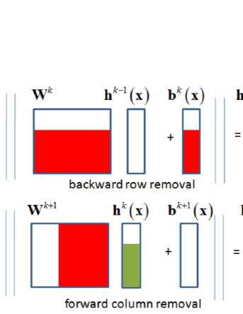
Figure 1: Example of backward and forward unit pruning. We use $\left\|.\right\|$ to indicate the $\mathrm{relu}\left(.\right)$ activation function. Based on knowledge that some unit activations ${\bf{h}}^{k}\left({\bf{x}}\right)$ are zero (indicated in green), we can reduce the parameters of ${\bf{W}}^{k}$, ${\bf{W}}^{k+1}$ and ${\bf{b}}^{k}$ (indicated in red).

2 Forward and backward unit pruning for object detection

Consider the original neural network $f\left({x;\theta}\right)$, where $\theta$ are the network parameters. We wish to compute a network defined by parameters $\theta^{*}$ for which:

$$f\left({x;\theta^{*}}\right)\approx f\left({x;\theta}\right)\forall x\in C$$ (1)

where $\left|{\theta^{*}}\right|<\left|\theta\right|$ (i.e. the number of parameters in $\theta^{*}$ is considerably lower than in the original network). In the case of object detection we will use the unit activations of the entire image to prune the network which will be applied to all the bounding box proposals. This is based on the observation that for some layers, nodes with zero activations on the whole image cannot have nonzero activation on any bounding box in the image.

The hidden layer activation of a fully connected layer $k$ can be written as:

$${\bf{h}}^{k}\left({\bf{x}}\right)=\mathrm{relu}({{\bf{b}}^{k}+{\bf{W}}^{k}{\bf{h}}^{k-1}\left({\bf{x}}\right)})$$ (2)

where ${\bf{b}}^{k}$ and ${\bf{W}}$ are the biases and weights of the $k$-th layer, and $\mathrm{relu}(\cdot)$ indicates the rectified linear activation function. We first consider how knowledge of the absence of node activations in the image can be translated into a network with fewer parameters. We consider two cases: backward and forward unit pruning, as illustrated in Fig. 1.

Backward unit pruning:   Without loss of generality, we order the activations in layer $h^{k}$ so that the $q$ non-active, zero nodes are at the end of vector $h^{k}$. Then we can write:

$$\left[{{\bf{h}}^{k}\left({\bf{x}}\right)_{1:\left({n-q}\right)};{\bf{0}}_{q,1}}\right]=\mathrm{relu}\left({\left[{{\bf{W}}^{k}_{1:\left({n-q}\right),1:m};{\bf{0}}_{q,m}}\right]{\bf{h}}^{k-1}\left({\bf{x}}\right)+\left[{{\bf{b}}^{k}_{{}_{1:\left({n-q}\right)}};{\bf{0}}_{q,1}}\right]}\right)$$ (3)

where we use ${\bf{0}}_{m,n}$ to indicate the zero-matrix of dimension $m$ by $n$, and subscripts are used to indicate a selection of indices from the original vector or matrix. We use $\left[{.,.}\right]$ for horizontal and $\left[{.;.}\right]$ for vertical concatenation (following Matlab convention). Eq. 3 shows that backward unit pruning allows us to remove from ${\bf{W}}^{k}$ and ${\bf{b}}^{k}$ an equal amount of rows as there are zeros in ${\bf{h}}^{k}$ – without changing the output of the network.

Forward unit pruning:   Here we look how the zeros in the activation ${\bf{h}}^{k}$ can be exploited to remove parameters from the following layer. The activation in layer $k+1$ can be written:

$${\bf{h}}^{k+1}\left({\bf{x}}\right)=\mathrm{relu}\left({\left[{{\bf{W}}^{k+1}_{1:p,1:\left({n-q}\right)},{\bf{0}}_{p,q}}\right]\left[{{\bf{h}}^{k}\left({\bf{x}}\right)_{1:\left({p-q}\right)};{\bf{0}}_{q,1}}\right]+{\bf{b}}^{k+1}}\right)$$ (4)

In this case, the zeros in ${\bf{h}}^{k}$ result in the removal of columns from ${\bf{W}}^{k+1}$. These can be removed without changing the output of the network.

In practice there might only be a few zero activation in the image and therefore we consider all node activations which are below a certain threshold to be zero. This allows us to further increase the parameter reduction of the network $f\left({x;\theta^{*}}\right)$ but at the cost of slight deviations from the original network $f\left({x;\theta}\right)$. We also note that although notations are about fully-connected layers for simplicity, our proposal would also be applicable to convolutional layers too.

3 Results and Conclusions

We evaluate our proposed methods on the VOC PASCAL 2007 dataset (Everingham et al. (2010)) with the fast R-CNN framework by Girshick (2015). The VOC 2007 has a total of 24,640 annotated objects for training, with an average of 2.5 objects per image, and in the test set an average of 2.4 objects per image. The Fast R-CNN framework is fit for our purposes since it first passes the image through all the convolutional layers to later use the extracted feature maps with the corresponding bounding boxes which we want to evaluate (usually 1,000+ boxes). The network used a modification of the VGG16 network (Simonyan & Zisserman (2014)).

Forward pruning.   Our first experiment uses forward unit pruning on the pool5 layer of the VGG16 network to reduce the number of parameters of the fc6 layer. This is the layer with highest percentage of parameters (38.7% parameters in the network). The pool5 layer has $512\times 7\times 7$ outputs, where the first dimension represents the feature maps, and the second and third dimensions are spatial dimensions (smaller than the original image size because of the resizing at each pooling layer). In order to decide which activations to prune, we first pass the whole image through the network and observe the activations at each unit in pool5. We sum over the spatial dimensions and apply a threshold to select units to prune from the network before applying it to all bounding boxes.

Figure 2: Performance loss as a function of parameter reduction.

Results show an initial minor improvement in the performance of the framework when removing parameters (see Fig. 2). The lack of propagation through the network of very low value activations could be the cause of the small difference in performance. Then, for reductions of 25-40% of the parameters on layer fc6, we obtain a mAP loss of less than 1. From that point on, further removal of parameters leads to higher loss. This happens because the activations removed start to be too relevant for the network’s discriminative power.

Backward pruning.   The second experiment applies backward unit pruning to the fc8 layer to reduce the number of parameters from the weight and bias matrices used to compute the network outputs. In this case, we use an image classifier (VGG16 deep features based) to decide which classes (activations) would be more likely to appear in the original image. Based on that classification, we adopt a top-$N$ strategy where we keep the $N$ classes with higher probability from the image classifier and remove the rest. This reduction affects the weight and bias matrices of the fc8, which would no longer propagate into the following layers (the softmax in this case). In this case, results keeping 6 or more classes (reductions of 0-70%) show a mAP loss of less than 1. However, performance starts dropping after because of images having more classes present than classes kept. It should be noted that only a small percentage of the total parameters of the network are in fc8. However, when considering object detection with thousands of classes, the relevance of this layer is comparable to fc6.

Conclusions.   We have presented a method to prune units in neural networks for object detection through analysis of unit activation on the entire image. We show that for some layers up to 40% of the parameters can be removed with minimal impact on performance. We are interested in combining our method with other parameter reduction methods such as Xue et al. (2013). Also applying our method to other types of layers (e.g. convolutional) and evaluating on datasets with very many labels are promising research directions. In addition, we are interested in applying our method to semantic segmentation where, similarly as in our problem, a redundant network is applied to every pixel.

Acknowledgments

This work is funded by the Projects TIN2013-41751-P of the Spanish Ministry of Science, the Catalan project 2014 SGR 221 and the CHIST ERA project PCIN-2015-226. We gratefully acknowledge the support of NVIDIA.

References

- Ba & Caruana (2014) Jimmy Ba and Rich Caruana. Do deep nets really need to be deep? In Advances in neural information processing systems (NIPS), pp. 2654–2662, 2014.
- Bucila et al. (2006) C Bucila, R Caruana, and A Niculescu-Mizil. Model compression: Making big, slow models practical. In Proc. of the 12th International Conf. on Knowledge Discovery and Data Mining (KDD’06), 2006.
- Everingham et al. (2010) Mark Everingham, Luc Van Gool, Christopher KI Williams, John Winn, and Andrew Zisserman. The pascal visual object classes (voc) challenge. International journal of computer vision, 88(2):303–338, 2010.
- Girshick (2015) Ross Girshick. Fast r-cnn. In Proceedings of the IEEE International Conference on Computer Vision, pp. 1440–1448, 2015.
- Hinton et al. (2015) Geoffrey Hinton, Oriol Vinyals, and Jeff Dean. Distilling the knowledge in a neural network. arXiv preprint arXiv:1503.02531, 2015.
- Romero et al. (2014) Adriana Romero, Nicolas Ballas, Samira Ebrahimi Kahou, Antoine Chassang, Carlo Gatta, and Yoshua Bengio. Fitnets: Hints for thin deep nets. CoRR, abs/1412.6550, 2014. URL http://arxiv.org/abs/1412.6550.
- Simonyan & Zisserman (2014) Karen Simonyan and Andrew Zisserman. Very deep convolutional networks for large-scale image recognition. arXiv preprint arXiv:1409.1556, 2014.
- Xue et al. (2013) Jian Xue, Jinyu Li, and Yifan Gong. Restructuring of deep neural network acoustic models with singular value decomposition. In INTERSPEECH, pp. 2365–2369, 2013.