Periods and Superstring Amplitudes

Abstract

Scattering amplitudes which describe the interaction of physical states play an important role in determining physical observables. In string theory the physical states are given by vibrations of open and closed strings and their interactions are described (at the leading order in perturbation theory) by a world–sheet given by the topology of a disk or sphere, respectively. Formally, for scattering of $N$ strings this leads to $N\!-\!3$–dimensional iterated real integrals along the compactified real axis or $N\!-\!3$–dimensional complex sphere integrals, respectively. As a consequence the physical observables are described by periods on ${\cal M}_{0,N}$ – the moduli space of Riemann spheres of $N$ ordered marked points. The mathematical structure of these string amplitudes share many recent advances in arithmetic algebraic geometry and number theory like multiple zeta values, single–valued multiple zeta values, Drinfeld, Deligne associators, Hopf algebra and Lie algebra structures related to Grothendiecks Galois theory. We review these results, with emphasis on a beautiful link between generalized hypergeometric functions describing the real iterated integrals on ${\cal M}_{0,N}({\bf R})$ and the decomposition of motivic multiple zeta values. Furthermore, a relation expressing complex integrals on ${\cal M}_{0,N}({\bf C})$ as single–valued projection of iterated real integrals on ${\cal M}_{0,N}({\bf R})$ is exhibited.

1 Introduction

During the last years a great deal of work has been addressed to the problem of revealing and understanding the hidden mathematical structures of scattering amplitudes in both field– and string theory. Particular emphasis on their underlying geometric structures seems to be especially fruitful and might eventually yield an alternative way of constructing perturbative amplitudes by methods residing in arithmetic algebraic geometry . In such a framework physical quantities are given by periods (or more generally by $L$–functions) typically describing the volume of some polytope or integrals of a discriminantal configuration (a configuration of multivariate hyperplanes). The mathematical quantities which occur in string amplitude computations are periods which relate to fundamental objects in number theory and algebraic geometry. A period is a complex number whose real and imaginary parts are given by absolutely convergent integrals of rational functions with rational coefficients over domains in ${\bf R}^{n}$ described by polynomial inequalities with rational coefficients. More generally, periods are values of integrals of algebraic differential forms over certain chains in algebraic varieties Kontsevich . E.g. in quantum field theory the coefficients of the Laurent series in the parameter $\epsilon=\frac{1}{2}(4\!-\!D)$ of dimensionally regulated Feynman integrals are numerical periods in the Euclidian region with all ratios of invariants and masses having rational values BognerMN . Furthermore, the power series expansion in the inverse string tension $\alpha^{\prime}$ of tree–level superstring amplitudes yields iterated integrals OprisaWU ; StiebergerTE ; BroedelTTA , which are periods of the moduli space ${\cal M}_{0,N}$ of genus zero curves with $N$ ordered marked points GM and integrate to ${\bf Q}$–linear combinations of multiple zeta values (MZVs) BrownQJA ; Terasoma . Similar considerations BL are expected to hold at higher genus in string perturbation theory, cf. BroedelVLA for some recent investigations at one–loop. At any rate, the analytic dependence on the inverse string tension $\alpha^{\prime}$ of string amplitudes furnishes an extensive and rich mathematical structure, which is suited to exhibit and study modern developments in number theory and arithmetic algebraic geometry.

The forms and chains entering the definition of periods may depend on parameters (moduli). As a consequence the periods satisfy linear differential equations with algebraic coefficients. This type of differential equations is known as generalized Picard–Fuchs equations or Gauss–Manin systems. A subclass of the latter describes the $A$–hypergeometric system or Gelfand–Kapranov–Zelevinsky (GKZ) system relevant to tree–level string scattering. One notorious example of periods are multivariate (multidimensional) or generalized hypergeometric functions. In the non–resonant case the solutions of the GKZ system can be represented by generalized Euler integrals GKZ , which appear as world–sheet integrals in superstring tree–level amplitudes and integrate to multiple Gaussian hypergeometric functions OprisaWU . Other occurrences of periods as physical quantities are string compactifications on Calabi–Yau manifolds. According to Batyrev the period integrals of Calabi–Yau toric varieties are also governed by GKZ systems. Therefore, the GKZ system is ubiquitous to functions describing physical effects in string theory as periods.

2 Periods on $\vec{{\cal M}_{0,N}}$

The object of interest is the moduli space ${\cal M}_{0,N}$ of Riemann spheres (genus zero curves) of $N\geq 4$ ordered marked points modulo the action of $PSL(2,{\bf C})$ on those points. The connected manifold ${\cal M}_{0,N}$ is described by the set of $N$–tuples of distinct points $(z_{1},\ldots,z_{N})$ modulo the action of $PSL(2,{\bf C})$ on those points. As a consequence with the choice

$$z_{1}=0,\ \ \ z_{N-1}=1,\ \ \ z_{N}=\infty$$ (2.1)

there is a unique representative

$$(z_{1},\ldots,z_{N})=(0,t_{1},\ldots,t_{N-3},1,\infty)$$ (2.2)

of each equivalence class of ${\cal M}_{0,N}$

$${\cal M}_{0,N}\simeq\{\ (t_{1},\ldots,t_{N-3})\in\left({\bf P}^{1}\backslash\{0,1,\infty\}\right)^{N-3}\ |\ t_{i}\neq t_{j}\ \mbox{for all}\ i\neq j\ \}\ ,$$ (2.3)

and the dimension of ${\cal M}_{0,N}({\bf C})$ is $N-3$. On the other hand, the real part of (2.3) describing the space of points

$${\cal M}_{0,N}({\bf R}):=\{(0,t_{1},\ldots,t_{N-3},1,\infty)\ |\ t_{i}\in{\bf R}\}$$ (2.4)

is not connected. Up to dihedral permutation each of its $\frac{1}{2}(N-1)!$ connected components (open cells $\gamma$)

$$\gamma=(z_{1},z_{2},\ldots,z_{N})$$ (2.5)

is completely described by the (real) ordering of the $N$ marked points

$$z_{1}<z_{2}<\ldots<z_{N}\ ,$$ (2.6)

with:

$$\bigcup_{i=1}^{N}\{z_{i}\}=\{0,t_{1},\ldots,t_{N-3},1,\infty\}\ .$$ (2.7)

In the compactification $\overline{\cal M}_{0,N}({\bf R})$ the components $\gamma$ become closed cells. Each cell corresponds to a triangulation of a regular polygon with $N$ sides. The number of triangulations is given by $C_{N-2}=\frac{2^{N-2}(2N-5)!!}{(N-1)!}$ (with $C_{N}$ the Catalan number). In total an underlying $K_{N-1}$ associahedron (Stasheff polytope) can naturally be associated with each vertex describing one triangulation BrownQJA . The standard cell of ${\cal M}_{0,N}$ is denoted by $\delta$ and given by the set of real marked points $(z_{1},z_{2},\ldots,z_{N})=(0,t_{1},t_{2},\ldots,t_{N-3},1,\infty)$ on ${\cal M}_{0,N}$ subject to the (canonical) ordering (2.6), i.e.:

$$\delta=\{\ t_{l}\in{\bf R}\ |\ 0<t_{1}<t_{2}<\ldots<t_{N-3}<1\ \}\ .$$ (2.8)

A period on ${\cal M}_{0,N}$ is defined to be a convergent integral GM

$$\int_{\delta}\omega$$ (2.9)

over the standard cell (2.8) in ${\cal M}_{0,N}({\bf R})$ and $\omega\in H^{N-3}({\cal M}_{0,N})$ a regular algebraic $(N-3)$–form, which converges on $\delta$ and has no poles along $\overline{\delta}$. Every period on ${\cal M}_{0,N}$ is a ${\bf Q}$–linear combination of MZVs BrownQJA . Furthermore, every MZV can be written as (2.9).

To each cell $\gamma$ a unique $(N-3)$–form can be associated BCS

$$\omega_{\gamma}=\prod_{i=2}^{N}(z_{i}-z_{i-1})^{-1}\ dt_{1}\wedge\ldots\wedge dt_{N-3}\ ,$$ (2.10)

subject to (2.7) with $z_{l}=\infty$ dismissed in the product. The form (2.10) is unique up to scalar multiplication, holomorphic on the interior of $\gamma$ and has simple poles on the boundary of that cell. To a cell (2.6) in ${\cal M}_{0,N}({\bf R})$ modulo rotations an oriented $N$–gon ($N$–sided polygons) may be associated by labelling clockwise its sides with the marked points $(z_{1},z_{2},\ldots,z_{N})$. E.g. according to (2.6) the polygon with the cyclically labelled sides $\gamma=(0,1,t_{1},t_{3},\infty,t_{2})$ is identified with the cell $0<1<t_{1}<t_{3}<\infty<t_{2}$ in ${\cal M}_{0,6}({\bf R})$ and the corresponding cell form is:

$$\omega_{\gamma}=\pm\frac{dt_{1}dt_{2}dt_{3}}{(-t_{2})\ (t_{3}-t_{1})\ (t_{1}-1)}\ .$$

The cell form (2.10) refers to the ordering (2.6). A cyclic structure $\gamma$ corresponds to the cyclic ordering $(\gamma(1),\gamma(2),\ldots,\gamma(N))$ of the elements $\{1,2,\ldots,N\}$ and refers to the standard $N$–gon $(1,2,\ldots,N)$ modulo rotations. There is a unique ordering $\sigma$ of the $N$ marked points (2.2) as

$$z_{\sigma(1)}<z_{\sigma(2)}<\ldots<z_{\sigma(N)}\ .$$ (2.11)

with $\sigma(N)=N$ and compatible with the cyclic structure $\gamma$. The cell–form corresponding to $\gamma$ is defined as BCS

$$\omega_{\gamma}=\prod\limits_{i=2}^{N-1}\left(z_{\sigma(i)}-z_{\sigma(i-1)}\right)^{-1}dt_{1}\wedge\ldots\wedge dt_{N-3}\ .$$ (2.12)

E.g. for the cyclic structure $(2,5,1,6,4,3)$ the unique ordering $\sigma$ compatible with the latter and with $\sigma(6)=6$ is the ordering $(4,3,2,5,1,6)$, i.e. $\gamma=(t_{3},t_{2},t_{1},1,0,\infty)$.

In the following, we consider orderings (2.6) ($01$ cyclic structure $\gamma$) of the set $\bigcup_{i=1}^{N}\{z_{i}\}=\{0,t_{1},\ldots,t_{N-3},1,\infty\}$ with the elements $z_{1}=0$ and $z_{N-1}=1$ being consecutive, i.e. $\gamma=(0,1,\rho)$ with $\rho\in S_{N-2}$ some ordering of the $N-2$ points $\{t_{1},\ldots,t_{N-3},\infty\}$. The corresponding cell–function is given by

$$\omega_{\rho}=z_{\rho(2)}^{-1}\ \prod\limits_{i=3}^{N-2}\left(z_{\rho(i)}-z_{\rho(i-1)}\right)^{-1}dt_{1}\wedge\ldots\wedge dt_{N-3}\ \ \ ,\ \ \ \rho\in S_{N-2}\ ,$$ (2.13)

it is called $01$ cell–function BCS and its associated $N$–gon, in which the edge referring to $0$ appears next to that referring to $1$, is depicted in Fig. 1.

[width=0.35]polygon.eps

Figure 1: $N$–gon describing the $01$ cyclic structure $\gamma=(0,1,\rho)$.

The $(N-2)!$ $01$ cell–functions (2.13) generate the top–dimensional cohomology group $H^{N-3}({\cal M}_{0,N})$ of ${\cal M}_{0,N}$ by constituting a basis of $H^{N-3}({\cal M}_{0,N},{\bf Q})$, i.e. BCS :

$$\dim H^{N-3}({\cal M}_{0,N},{\bf Q})=(N-2)!\ .$$ (2.14)

As a consequence the cohomology group $H^{N-3}({\cal M}_{0,N})$ is canonically isomorphic to the subspace of polygons having the vertex (edge) $0$ adjacent to edge $1$ BCS .

Generically, in terms of cells a period (2.9) on ${\cal M}_{0,N}$ may be defined as the integral BCS

$$\int_{\beta}\omega_{\gamma}$$ (2.15)

over the cell $\beta$ in ${\cal M}_{0,N}({\bf R})$ and the cell–form $\omega_{\gamma}$ with the pair $(\beta,\gamma)$ referring to some polygon pair. Therefore, generically the cell–forms (2.10) integrated over cells (2.5) give rise to periods on ${\cal M}_{0,N}$, which are ${\bf Q}$–linear combinations of MZV. By changing variables the period integral (2.15) can be brought into an integral over the standard cell $\delta$ parameterized in (2.8). To obtain a convergent integral (2.15) in BCS certain linear combinations of $01$ cell–forms (2.13) (called insertion forms) have been constructed with the properties of having no poles along the boundary of the standard cell $\delta$ and converging on the closure $\overline{\delta}$. E.g. in the case of ${\cal M}_{0,5}$ the cell–form $\omega_{\gamma}$ corresponding to the cell $\gamma=(0,1,t_{1},\infty,t_{2})$ can be integrated over the compact standard cell $\overline{\delta}$ defined in (2.8)

$$\int_{\overline{\delta}}\omega_{\gamma}=\int_{0\leq t_{1}\leq t_{2}\leq 1}\frac{dt_{1}dt_{2}}{(1-t_{1})\ t_{2}}=\zeta_{2}\ ,$$ (2.16)

with the period $\zeta_{2}$ following from the general definition for the Riemann zeta function:

$$\zeta_{a}=\sum_{k=1}^{\infty}k^{-a}\ \ \ ,\ \ \ a\in{\bf N},\ a\geq 2\ .$$ (2.17)

3 Volume form and period matrix on $\vec{{\cal M}_{0,N}}$

For a regular algebraic $(N-3)$–form $\omega_{\delta}$ on ${\cal M}_{0,N}$ conditions exist for the integral (2.9) over the standard cell $\delta$ to converge. The set of all regular $(N-3)$–forms can be written in terms of the canonical cyclically invariant form BrownQJA :

$$\omega_{\delta}=\frac{dt_{1}\wedge\ldots\wedge dt_{N-3}}{t_{2}\ (t_{3}-t_{1})\ (t_{4}-t_{2})\cdot\ldots\cdot(t_{N-3}-t_{N-5})\ (1-t_{N-4})}\ .$$ (3.18)

(Up to multiplication by ${\bf Q}^{+}$) this form is the canonical volume form on ${\cal M}_{0,N}({\bf R})$ without zeros or poles along the standard cell (2.8). An algebraic volume form $\Omega$ on ${\cal M}_{0,N}({\bf R})$ may be supplemented by the $PSL(2,{\bf C})$ invariant factor $\prod_{i<j}^{N-1}|z_{i}-z_{j}|^{s_{ij}}$ (subject to (2.1) and with some conditions on the parameter $s_{ij}$, which turn into physical conditions, cf. (6.101)) as

$$\Omega=\frac{dt_{1}\wedge\ldots\wedge dt_{N-3}}{t_{2}\ (t_{3}-t_{1})\ (t_{4}-t_{2})\cdot\ldots\cdot(t_{N-3}-t_{N-5})\ (1-t_{N-4})}\ \left(\prod_{i<j}^{N-1}|z_{i}-z_{j}|^{s_{ij}}\right)\ ,$$ (3.19)

with $s_{ij}\in{\bf Z}$. The form (3.19) gives rise to the family of periods $\int_{\overline{\delta}}\Omega$ of ${\cal M}_{0,N}$

$$I_{\delta}(a,b,c)=\int_{\overline{\delta}}dt_{1}\cdot\ldots\cdot dt_{N-3}\ \prod\limits_{i=1}^{N-3}t_{i}^{a_{i}}\ (1-t_{i})^{b_{i}}\ \prod\limits_{1\leq i<j\leq N-3}(t_{i}-t_{j})^{c_{ij}}\ ,$$ (3.20)

for suitable choices of integers $a_{i},b_{i},c_{ij}\in{\bf Z}$ such that the integral converges. The latter refers to the compactified standard cell $\delta$ defined in (2.8). It has been shown by Brown and Terasoma, that integrals of the form (3.20) yield linear combinations of MZVs with rational coefficients. In cubical coordinates $x_{1}=\frac{t_{1}}{t_{2}},\ x_{2}=\frac{t_{2}}{t_{3}},\ldots,x_{N-4}=\frac{t_{N-4}}{t_{N-3}},\ x_{N-3}=t_{N-3}$ parameterizing the integration region (2.8) as $t_{k}=\prod_{l=k}^{N-3}x_{l},\ k=1,\ldots,N-3$ with $0<x_{i}<1$, the integral (3.20) becomes

$$I_{\delta}(a^{\prime},b^{\prime},c^{\prime})=\left(\prod_{i=1}^{N-3}\ \int^{1}_{0}dx_{i}\right)\ \prod_{j=1}^{N-3}\,x_{j}^{a^{\prime}_{j}}\ (1-x_{j})^{b^{\prime}_{j}}\ \prod_{l=j+1}^{N-3}\ \left(\ 1\ -\ \prod_{k=j}^{l}x_{k}\ \right)^{c_{jl}^{\prime}}\ ,$$ (3.21)

with some integers $a_{i}^{\prime},b_{i}^{\prime},c_{ij}^{\prime}\in{\bf Z}$.

Moreover, the form (3.19) can be generalized to the family of real period integrals $\int_{\overline{\delta}}\Omega$ on $\overline{\delta}$, with $s_{ij}\in{\bf R}$. Then, Taylor expanding (3.19) w.r.t. $s_{ij}$ at integral points $s_{ij}\in{\bf Z}^{+}$ yields coefficients representing period integrals of the form (3.20). Similar observations have been made in OprisaWU ; StiebergerTE when computing $\alpha^{\prime}$–expansions of string amplitudes which can be described by integrals of the type (3.21). In this setup the additional $PSL(2,{\bf C})$ invariant factor $\prod_{i<j}^{N-1}|z_{i}-z_{j}|^{\alpha^{\prime}s_{ij}}$ represents the so–called Koba–Nielsen factor with the parameter $\alpha^{\prime}$ being the inverse string tension and the kinematic invariants $s_{ij}$ specified in (6.101).

Similarly to (3.19) in the following let us consider all the $(N-2)!$ $01$ cell–forms (2.13) supplemented by the $PSL(2,{\bf C})$ invariant factor $\prod_{i<j}^{N-1}|z_{i}-z_{j}|^{\alpha^{\prime}s_{ij}}$ and integrated over the standard cell $\delta$ in ${\cal M}_{0,N}({\bf R})$, i.e.:

$$\int_{\delta}\left(\prod_{i<j}^{N-1}|z_{i}-z_{j}|^{\alpha^{\prime}s_{ij}}\right)\ \omega_{\rho}=\int_{\delta}\frac{dt_{1}\wedge\ldots\wedge dt_{N-3}}{z_{\rho(2)}\ \prod\limits_{i=3}^{N-2}\left(z_{\rho(i)}-z_{\rho(i-1)}\right)}\ \left(\prod_{i<j}^{N-1}|z_{i}-z_{j}|^{\alpha^{\prime}s_{ij}}\right)\ \ \ ,\ \ \ \rho\in S_{N-2}\ .$$ (3.22)

Integration by part allows to express the $(N-2)!$ integrals (3.22) in terms of a basis of $(N-3)!$ integrals, i.e.:

$$\dim H^{N-3}({\cal M}_{0,N},{\bf R})=(N-3)!\ .$$ (3.23)

For a given cell $\pi$ in ${\cal M}_{0,N}({\bf R})$ we can choose the $01$ cell–form $\omega_{\gamma}$ with $\gamma=(0,1,\infty,\rho),\ \rho\in S_{N-3}$ and the following basis (subject to (2.1)) BroedelTTA

$$Z_{\pi}^{\rho} := Z_{\pi}(1,\rho(2,3,\ldots,N-2),N,N-1)$$

$$= \displaystyle{\int_{\pi}\left(\prod_{i=2}^{N-2}dz_{i}\right)\ \frac{\prod\limits_{i<j}^{N-1}|z_{ij}|^{\alpha^{\prime}s_{ij}}}{z_{1\rho(2)}z_{\rho(2),\rho(3)}\ldots z_{\rho(N-3),\rho(N-2)}}\ \ \ ,\ \ \ \pi,\rho\in S_{N-3}\ ,}$$

with

$$z_{ij}:=z_{i}-z_{j}\ ,$$ (3.25)

and $\rho$ describing some ordering of the $N-3$ points $\bigcup_{i=2}^{N-2}\{z_{i}\}=\{t_{1},\ldots,t_{N-3}\}$ along the $N$–gon depicted in Fig. 2.

[width=0.35]polygon2.eps

Figure 2: $N$–gon describing the cyclic structure $\gamma=(0,1,\infty,\rho)$.

The iterated integrals (3) represent generalized Euler (Selberg) integral and integrate to multiple Gaussian hypergeometric functions OprisaWU . Furthermore, the integrals (3) can also be systematized within the framework of Aomoto-Gelfand hypergeometric functions or GKZ structures GKZ .

The integrals (3) can be Taylor expanded w.r.t. $\alpha^{\prime}$ around the point $\alpha^{\prime}=0$, e.g.:

$$\begin{array}[]{lcl}&&\displaystyle{\int\limits_{\delta}\left(\prod_{l=2}^{3}dz_{l}\right)\ \frac{\prod\limits_{i<j}^{4}|z_{ij}|^{\alpha^{\prime}s_{ij}}}{z_{12}\ z_{23}\ z_{41}}}\\[19.91692pt] &=&\displaystyle{\alpha^{\prime-2}\ \left(\frac{1}{s_{12}s_{45}}+\frac{1}{s_{23}s_{45}}\right)+\zeta_{2}\ \left(1-\frac{s_{34}}{s_{12}}-\frac{s_{12}}{s_{45}}-\frac{s_{23}}{s_{45}}-\frac{s_{51}}{s_{23}}\right)+{\cal O}(\alpha^{\prime})\ .}\end{array}$$ (3.26)

Techniques for computing $\alpha^{\prime}$ expansions for the type of integrals (3) have been exhibited in OprisaWU ; StiebergerTE , systematized in BroedelTTA , and pursued in Puhlfuerst:2015gta . In fact, the lowest order contribution of (3) in the Taylor expansion around the point $\alpha^{\prime}=0$ is given by

$$\left.Z\right|_{\alpha^{\prime 3-N}}=(-1)^{N-3}\ S^{-1}\ ,$$ (3.27)

with the kernel KawaiXQ ; BernSV ; Bohr

$$S[\rho|\sigma]:=S[\,\rho(2,\ldots,N-2)\,|\,\sigma(2,\ldots,N-2)\,]=\alpha^{\prime N-3}\ \prod_{j=2}^{N-2}\Big{(}\,s_{1,j_{\rho}}\ +\ \sum_{k=2}^{j-1}\theta(j_{\rho},k_{\rho})\,s_{j_{\rho},k_{\rho}}\,\Big{)}\ ,$$ (3.28)

with $j_{\rho}=\rho(j)$ and $\theta(j_{\rho},k_{\rho})=1$ if the ordering of the legs $j_{\rho},k_{\rho}$ is the same in both orderings $\rho(2,\ldots,N-2)$ and $\sigma(2,\ldots,N-2)$, and zero otherwise. The matrix elements $S[\rho|\sigma]$ are polynomials of the order $N-3$ in the parameters (6.101).

A natural object to define is the $(N-3)!\times(N-3)!$–matrix

$$F_{\pi\sigma}=(-1)^{N-3}\ \sum_{\rho\in S_{N-3}}Z_{\pi}(\rho)\ S[\rho|\sigma]\ ,$$ (3.29)

which according to (3.27) satisfies:

$$\left.F\right|_{\alpha^{\prime 3-N}}=1\ .$$ (3.30)

The matrix $F$ has rank

$${\rm rk}(F)=(N-3)!$$ (3.31)

and represents the period matrix of ${\cal M}_{0,N}$ Sasha .

In SS it has been observed, that $F$ can be written in the following way

$$F=P\ Q\ :\exp\left\{\sum\limits_{n\geq 1}\zeta_{2n+1}\ M_{2n+1}\right\}:\ ,$$ (3.32)

with the Riemann zeta–functions (2.17). This decomposition is guided by its organization w.r.t. multiple zeta values (MZVs) $\zeta_{n_{1},\ldots,n_{r}}$ as

$$\begin{array}[]{lcl}M_{2n+1}&=&\displaystyle{\left.F\right|_{\zeta_{2n+1}}\ ,}\\[8.53581pt] P_{2n}&=&\displaystyle{\left.F\right|_{\zeta_{2}^{n}}\ ,}\end{array}$$ (3.33)

with:

$$P = 1+\sum_{n\geq 1}\zeta_{2}^{n}\ P_{2n}\ ,$$ (3.34)

$$Q = \displaystyle{1+\sum_{n\geq 8}Q_{n}=1+\frac{1}{5}\ \zeta_{3,5}\ [M_{5},M_{3}]+\left\{\ \frac{3}{14}\ \zeta_{5}^{2}+\frac{1}{14}\ \zeta_{3,7}\ \right\}\ [M_{7},M_{3}]}$$ (3.35)

$$+ \displaystyle{\left\{\ 9\ \zeta_{2}\ \zeta_{9}+\frac{6}{25}\ \zeta_{2}^{2}\ \zeta_{7}-\frac{4}{35}\ \zeta_{2}^{3}\ \zeta_{5}+\frac{1}{5}\ \zeta_{3,3,5}\ \right\}\ [M_{3},[M_{5},M_{3}]]+\ldots\ .}$$

MZVs are generalizations of single zeta functions (2.17)

$$\zeta_{n_{1},\ldots,n_{r}}:=\zeta(n_{1},\ldots,n_{r})=\sum\limits_{0<k_{1}<\ldots<k_{r}}\ \prod\limits_{l=1}^{r}k_{l}^{-n_{l}}\ \ \ ,\ \ \ n_{l}\in{\bf N}^{+}\ ,\ n_{r}\geq 2\ ,$$ (3.36)

with $r$ specifying its depth and $w=\sum_{l=1}^{r}n_{l}$ denoting its weight. Hence, all the information is kept in the matrices $P$ and $M$ and the particular form of $Q$. The entries of the matrices $M_{2n+1}$ are polynomials in $s_{ij}$ of degree $2n+1$ (and hence of the order $\alpha^{\prime 2n+1}$), while the entries of the matrices $P_{2n}$ are polynomials in $s_{ij}$ of degree $2n$ (and hence of the order $\alpha^{\prime 2n}$). E.g. for $N=5$ we have

$$P=\alpha^{\prime 2}\ \left(\begin{array}[]{lcl}-s_{34}s_{45}+s_{12}\ (s_{34}-s_{51})&s_{13}\ s_{24}\\ s_{12}\ s_{34}&(s_{12}+s_{23})\ (s_{23}+s_{34})-s_{45}s_{51}\end{array}\right)\ ,$$ (3.37)

and

$$M_{3}=\alpha^{\prime 3}\ \left(\begin{array}[]{lcl}m_{11}&m_{12}\\ m_{21}&m_{22}\end{array}\right)\ ,$$ (3.38)

with:

$$\begin{array}[]{lcl}m_{11}&=&s_{34}\ [\ -s_{12}\ (s_{12}+2s_{23}+s_{34})+s_{34}s_{45}+s_{45}^{2}\ ]+s_{12}s_{51}\ (s_{12}+s_{51})\ ,\\[2.84526pt] m_{12}&=&-s_{13}\ s_{24}\ (s_{12}+s_{23}+s_{34}+s_{45}+s_{51})\ ,\\[2.84526pt] m_{21}&=&s_{12}\ s_{34}\ [\ s_{12}+s_{23}+s_{34}-2\ (s_{45}+s_{51})\ ]\ ,\\[2.84526pt] m_{22}&=&(s_{23}+s_{34})\ [\ (s_{12}+s_{23})(s_{12}+s_{34})-2\ s_{12}s_{45}\ ]\\[2.84526pt] &&-[\ 2s_{12}s_{34}-s_{45}^{2}+2s_{23}\ (s_{34}+s_{45})\ ]s_{51}+s_{45}s_{51}^{2}\ .\end{array}$$ (3.39)

As we shall see in section 5 the form (3.32) is bolstered by the algebraic structure of motivic MZVs. The form (3.32) exactly appears in F. Browns decomposition of motivic MZVs Brown . In section 6 we shall demonstrate, that the period matrix $F$ has also a physical meaning describing scattering amplitudes of open and closed strings.

4 Motivic and single–valued multiple zeta values

MZVs (3.36) can be represented as period integrals. With the iterated integrals of the following form

$$I_{\gamma}(a_{0};a_{1},\ldots,a_{n};a_{n+1})=\int_{\Delta_{n},\gamma}\frac{dz_{1}}{z_{1}-a_{1}}\ldots\frac{dz_{n}}{z_{n}-a_{n}}\ ,$$ (4.40)

with $\gamma$ a path in $M={\bf C}/\{a_{1},\ldots,a_{n}\}$ with endpoints $\gamma(0)=a_{0}\in M,\ \gamma(1)=a_{n+1}\in M$ and $\Delta_{n,\gamma}$ a simplex consisting of all ordered $n$–tuples of points $(z_{1},\ldots,z_{n})$ on $\gamma$ and for the map

$$\rho(n_{1},\ldots,n_{r})=10^{n_{1}-1}\ldots 10^{n_{r}-1}\ ,$$ (4.41)

with $n_{r}\geq 2$ Kontsevich observed that

$$\zeta_{n_{1},\ldots,n_{r}} = (-1)^{r}\ I_{\gamma}(0;\rho(n_{1}\ldots n_{r});1)$$ (4.42)

$$= \displaystyle{(-1)^{r}\ \int\limits_{0\leq t_{1}\leq\ldots\leq t_{n}\leq 1}\frac{dt_{1}}{t_{1}-a_{1}}\ldots\frac{dt_{n}}{t_{n}-a_{n}}\ ,}$$

with the sequence of numbers $(a_{1},\ldots,a_{n})$ given by $(1,0^{n_{1}-1},\ldots,1,0^{n_{r}-1})$. Note, that the integral (4.42) defines a period. Furthermore, the numbers (3.36) arise as coefficients of the Drinfeld associator $Z(e_{0},e_{1})$ Drinii . The latter is a function in terms of the generators $e_{0}$ and $e_{1}$ of a free Lie algebra $g$ and is given by the non–commutative generating series of (shuffle–regularized) MZVs LeMurakami

$$Z(e_{0},e_{1})=\sum_{w\in\{e_{0},e_{1}\}^{\times}}\zeta(w)\ w\ ,$$ (4.43)

with the symbol $w\in\{e_{0},e_{1}\}^{\times}$ denoting a non–commutative word $w_{1}w_{2}\ldots$ in the letters $w_{i}\in\{e_{0},e_{1}\}$. Furthermore, we have the shuffle product $\zeta(w_{1})\zeta(w_{2})=\zeta(w_{1}\shuffle w_{2})$ and $\zeta(e_{0})=0=\zeta(e_{1})$ and $\zeta(e_{1}e_{0}^{n_{1}-1}\ldots e_{1}e_{0}^{n_{r}-1})=\zeta_{n_{1},\ldots,n_{r}}$. Explicitly, (4.43) becomes:

$$Z(e_{0},e_{1}) = \sum_{w\in\{e_{0},e_{1}\}^{\times}}\zeta(w)\ w=1+\zeta_{2}\ [e_{0},e_{1}]+\zeta_{3}\ (\ [e_{0},[e_{0},e_{1}]]-[e_{1},[e_{0},e_{1}]\ )$$

$$+ \zeta_{4}\ \Big{(}\ [e_{0},[e_{0},[e_{0},e_{1}]]]-\frac{1}{4}\ [e_{1},[e_{0},[e_{0},e_{1}]]]+[e_{1},[e_{1},[e_{0},e_{1}]]]+\frac{5}{4}\ [e_{0},e_{1}]^{2}\ \Big{)}$$

$$+ \zeta_{2}\ \zeta_{3}\ \Big{(}\ ([e_{0},[e_{0},e_{1}]]-[e_{1},[e_{0},e_{1}])\ [e_{0},e_{1}]+[e_{0},[e_{1},[e_{0},[e_{0},e_{1}]]]]$$

$$- [e_{0},[e_{1},[e_{1},[e_{0},e_{1}]]]]\ \Big{)}+\zeta_{5}\ \Big{(}\ [e_{0},[e_{0},[e_{0},[e_{0},e_{1}]]]]$$

$$- \frac{1}{2}\ [e_{0},[e_{0},[e_{1},[e_{0},e_{1}]]]]-\frac{3}{2}\ [e_{1},[e_{0},[e_{0},[e_{0},e_{1}]]]]+(e_{0}\leftrightarrow e_{1})\ \Big{)}+\ldots\ .$$ (4.45)

The set of integral linear combinations of MZVs (3.36) is a ring, since the product of any two values can be expressed by a (positive) integer linear combination of the other MZVs Zagier . There are many relations over ${\bf Q}$ among MZVs. We define the (commutative) ${\bf Q}$–algebra ${\cal Z}$ spanned by all MZVs over ${\bf Q}$. The latter is the (conjecturally direct) sum over the ${\bf Q}$–vector spaces ${\cal Z}_{N}$ spanned by the set of MZVs (3.36) of total weight $w=N$, with $n_{r}\geq 2$, i.e. ${\cal Z}=\bigoplus_{k\geq 0}{\cal Z}_{k}$. For a given weight $w\in{\bf N}$ the dimension $\dim_{\bf Q}({\cal Z}_{N})$ of the space ${\cal Z}_{N}$ is conjecturally given by $\dim_{\bf Q}({\cal Z}_{N})=d_{N}$, with $d_{N}=d_{N-2}+d_{N-3},\ N\geq 3$ and $d_{0}=1,\ d_{1}=0,\ d_{2}=1$ Zagier . Starting at weight $w=8$ MZVs of depth greater than one $r>1$ appear in the basis. By applying stuffle, shuffle, doubling, generalized doubling relations and duality it is possible to reduce the MZVs of a given weight to a minimal set. Strictly speaking this is explicitly proven only up to weight $26$ DataMine . For $D_{w,r}$ being the number of independent MZVs at weight $w>2$ and depth $r$, which cannot be reduced to primitive MZVs of smaller depth and their products, it is believed, that $D_{8,2}=1,D_{10,2}=1,\ D_{11,3}=1,\ D_{12,2}=1$ and $D_{12,4}=1$ Broadii . For $Z=\frac{{\cal Z}_{>0}}{{\cal Z}_{>0}\cdot{\cal Z}_{>0}}$ with ${\cal Z}_{>0}=\oplus_{w>0}{\cal Z}_{w}$ the graded space of irreducible MZVs we have: $dim(Z_{w})\equiv\sum_{r}D_{w,r}=1,0,1,0,1,1,1,1,2,2,3,3,4,5$ for $w=3,\ldots,16$, respectively Broadii ; DataMine .

An important question is how to decompose a MZV of a certain weight $w$ in terms of a given basis of the same weight $w$. E.g. for the decomposition

$$\zeta_{4,3,3}=\frac{4336}{1925}\ \zeta_{2}^{5}+\frac{1}{5}\ \zeta_{2}^{2}\zeta_{3}^{2}+10\ \zeta_{2}\zeta_{3}\zeta_{5}-\frac{49}{2}\ \zeta_{5}^{2}-18\ \zeta_{3}\zeta_{7}-4\ \zeta_{2}\zeta_{3,5}+\zeta_{3,7}$$ (4.46)

we wish to find a method to determine the rational coefficients. Clearly, this question cannot be answered within the space of MZV ${\cal Z}$ as we do not know how to construct a basis of MZVs for any weight. Eventually, we seek to answer the above question within the space ${\cal H}$ of motivic MZVs with the latter serving as some auxiliary objects for which we assume certain properties Brown . For this purpose the actual MZVs (3.36) are replaced by symbols (or motivic MZVs), which are elements of a certain algebra. We lift the ordinary MZVs $\zeta$ to their motivic versions $\zeta^{\mathfrak{m}}$ with the surjective projection (period map) Goncharov ; GoncharovBrown :

$$\rm per:\zeta^{\mathfrak{m}}\longrightarrow\zeta\ .$$ (4.47)

Furthermore, the standard relations among MZV (like shuffle and stuffle relations) are supposed to hold for the motivic MZVs $\zeta^{\mathfrak{m}}$. In particular, ${\cal H}$ is a graded Hopf algebra ${\cal H}$ with a coproduct $\Delta$, i.e.

$${\cal H}=\bigoplus_{n\geq 0}{\cal H}_{n}\ ,$$ (4.48)

and for each weight $n$ the Zagier conjecture is assumed to be true, i.e.  $\dim_{\bf Q}({\cal H}_{n})=d_{n}$. To explicitly describe the structure of the space ${\cal H}$ one introduces the (trivial) algebra–comodule:

$${\cal U}={\bf Q}\langle f_{3},f_{5},\ldots\rangle\ \otimes_{\bf Q}\ {\bf Q}[f_{2}]\ .$$ (4.49)

The multiplication on

$${\cal U}^{\prime}={\cal U}\big{/}f_{2}{\cal U}={\bf Q}\langle f_{3},f_{5},\ldots\rangle$$ (4.50)

is given by the shuffle product $\shuffle$

$$f_{i_{1}}\ldots f_{i_{r}}\shuffle f_{i_{r+1}}\ldots f_{i_{r+s}}=\sum_{\sigma\in{\Sigma}(r,s)}f_{i_{\sigma(1)}}\ldots f_{i_{\sigma(r+s)}}\ ,$$ (4.51)

${\Sigma}(r,s)=\{\sigma\in{\Sigma}(r+s)\ |\ \sigma^{-1}(1)<\ldots<\sigma^{-1}(r)\cap\sigma^{-1}(r+1)<\ldots<\sigma^{-1}(r+s)\}$. The Hopf–algebra ${\cal U}^{\prime}$ is isomorphic to the space of non–commutative polynomials in $f_{2i+1}$. The element $f_{2}$ commutes with all $f_{2r+1}$. Again, there is a grading ${\cal U}_{k}$ on ${\cal U}$, with $\dim({\cal U}_{k})=d_{k}$. Then, there exists a morphism $\phi$ of graded algebra–comodules

$$\phi:\ {\cal H}\longrightarrow{\cal U}\ ,$$ (4.52)

normalized by:

$$\phi\big{(}\zeta^{\mathfrak{m}}_{n}\big{)}=f_{n}\ \ \ ,\ \ \ n\geq 2\ .$$ (4.53)

Furthermore, (4.52) respects the shuffle multiplication rule (4.51):

$$\phi(x_{1}x_{2})=\phi(x_{1})\shuffle\phi(x_{2})\ \ \ ,\ \ \ x_{1},x_{2}\in{\cal H}\ .$$ (4.54)

The map (4.52) is defined recursively from lower weight and sends every motivic MZV $\xi\in{\cal H}_{N+1}$ of weight $N+1$ to a non–commutative polynomial in the $f_{i}$. The latter is given as series expansion up to weight $N+1$ w.r.t. the basis $\{f_{2r+1}\}$

$$\phi(\xi)=c_{N+1}\ f_{N+1}+\sum_{3\leq 2r+1\leq N}f_{2r+1}\ \xi_{2r+1}\in{\cal U}_{N+1}\ ,$$ (4.55)

with the coefficients $\xi_{2r+1}\in{\cal U}_{N-2r}$ being of smaller weight than $\xi$ and computed from the coproduct as follows. The derivation $D_{r}:{\cal H}_{m}\rightarrow{\cal A}_{r}\otimes{\cal H}_{m-r}$, with ${\cal A}={\cal H}/\zeta_{2}{\cal H}$ takes only a subset of the full coproduct, namely the weight $(r,m-r)$–part. Hence, $D_{2r+1}\xi$ gives rise to a weight $(2r+1,N-2r)$–part $x_{2r+1}\otimes y_{N-2r}\in{\cal A}_{2r+1}\otimes{\cal H}_{N-2r}$ and $\xi_{2r+1}:=c_{2r+1}^{\phi}(x_{2r+1})\cdot\phi(y_{N-2r})$ The operator $c_{2r+1}^{\phi}(x_{2r+1})$, with $x_{2r+1}\in{\cal A}_{2r+1}$ determines the rational coefficient of $f_{2r+1}$ in the monomial $\phi(x_{2r+1})\in{\cal U}_{2r+1}$. Note, that the right hand side of $\xi_{2r+1}$ only involves elements from ${\cal H}_{\leq N}$ for which $\phi$ has already been determined. On the other hand, the coefficient $c_{N+1}$ cannot be determined by this method unless we specify a basis $B$ and compute $\phi$ for this basis giving rise to the basis dependent map $\phi^{B}$. E.g. for the basis $B=\{\zeta_{2}^{\mathfrak{m}}\zeta_{3}^{\mathfrak{m}},\zeta_{5}^{\mathfrak{m}}\}$ we have $\phi^{B}(\zeta_{2}^{\mathfrak{m}}\zeta_{3}^{\mathfrak{m}})=f_{2}f_{3}$ and $\phi^{B}(\zeta_{5}^{\mathfrak{m}})=f_{5}$, while $\phi^{B}(\zeta^{\mathfrak{m}}_{2,3})=3f_{3}f_{2}+cf_{5}$ with $c$ undetermined.

To illustrate the procedure for computing the map (4.52) and determining the decomposition let us consider the case of weight $10$. First, we introduce a basis of motivic MZVs

$$B_{10}=\{\ \zeta^{\mathfrak{m}}_{3,7},\ \zeta^{\mathfrak{m}}_{3}\ \zeta^{\mathfrak{m}}_{7},\ (\zeta^{\mathfrak{m}}_{5})^{2},\ \zeta^{\mathfrak{m}}_{3,5}\ \zeta^{\mathfrak{m}}_{2},\ \zeta^{\mathfrak{m}}_{3}\ \zeta^{\mathfrak{m}}_{5}\ \zeta^{\mathfrak{m}}_{2},\ (\zeta^{\mathfrak{m}}_{3})^{2}\ (\zeta^{\mathfrak{m}}_{2})^{2},\ (\zeta^{\mathfrak{m}}_{2})^{5}\ \}\ ,$$ (4.57)

with $\dim(B_{10})=d_{10}$. Then for each basis element we compute (4.52):

$$\begin{array}[]{lcl}\displaystyle{\phi^{B}\left(\zeta^{\mathfrak{m}}_{3,7}\right)}&=&\displaystyle{-14\ f_{7}f_{3}-6\ f_{5}f_{5},\ \ \ \phi^{B}\left(\zeta^{\mathfrak{m}}_{3}\zeta^{\mathfrak{m}}_{7}\right)=f_{3}\shuffle f_{7}\ ,}\\[8.53581pt] \displaystyle{\phi^{B}\left((\zeta^{\mathfrak{m}}_{5})^{2}\right)}&=&\displaystyle{f_{5}\shuffle f_{5},\ \ \ \phi^{B}\left(\zeta^{\mathfrak{m}}_{3,5}\zeta^{\mathfrak{m}}_{2}\right)=-5\ f_{5}f_{3}f_{2}\ ,}\\[8.53581pt] \displaystyle{\phi^{B}\left(\zeta^{\mathfrak{m}}_{3}\zeta^{\mathfrak{m}}_{5}\zeta^{\mathfrak{m}}_{2}\right)}&=&\displaystyle{f_{3}\shuffle f_{5}f_{2},\ \ \ \phi^{B}\left((\zeta^{\mathfrak{m}}_{3})^{2}(\zeta^{\mathfrak{m}}_{2})^{2}\right)=f_{3}\shuffle f_{3}f_{2}^{2}\ ,}\\[8.53581pt] \displaystyle{\phi^{B}\left((\zeta^{\mathfrak{m}}_{2})^{5}\right)}&=&\displaystyle{f_{2}^{5}\ .}\end{array}\$$ (4.58)

The above construction allows to assign a ${\bf Q}$–linear combination of monomials to every element $\zeta^{\mathfrak{m}}_{n_{1},\ldots,n_{r}}$. The map (4.52) sends every motivic MZV of weight less or equal to $N$ to a non–commutative polynomial in the $f_{i}$’s. Inverting the map $\phi$ gives the decomposition of $\zeta^{\mathfrak{m}}_{n_{1},\ldots,n_{r}}$ w.r.t. the basis $B_{n}$ of weight $n$, with $n=\sum_{l=1}^{r}n_{l}$. We construct operators acting on $\phi(\xi)\in{\cal U}$ to detect elements in ${\cal U}$ and to decompose any motivic MZV $\xi$ into a candidate basis $B$. The derivation operators $\partial_{2n+1}:{\cal U}\rightarrow{\cal U}$ are defined as Brown :

$$\partial_{2n+1}(f_{i_{1}}\ldots f_{i_{r}})=\left\{\begin{array}[]{lcl}f_{i_{2}}\ldots f_{i_{r}},&i_{1}=2n+1\ ,\\ 0\ ,&\rm{otherwise}\ ,\end{array}\right.$$ (4.59)

with $\partial_{2n+1}f_{2}=0$. Furthermore, we have the product rule for the shuffle product:

$$\partial_{2n+1}(a\shuffle b)=\partial_{2n+1}a\shuffle b+a\shuffle\partial_{2n+1}b\ \ \ ,\ \ \ a,b\in{\cal U}^{\prime}\ .$$ (4.60)

Finally, $c_{2}^{n}$ takes the coefficient of $f_{2}^{n}$. By first determining the map (4.52) for a given basis $B_{n}$ we then can construct the motivic decomposition operator $\xi_{n}$ such that it acts trivially on this basis. This is established for the weight ten basis (4.58) in the following.

With the differential operator (4.59) we may consider the following operator

$$\begin{array}[]{lcl}\displaystyle{\xi_{10}}&=&\displaystyle{a_{0}\ (\zeta^{\mathfrak{m}}_{2})^{5}+a_{1}\ (\zeta^{\mathfrak{m}}_{2})^{2}\ (\zeta^{\mathfrak{m}}_{3})^{2}+a_{2}\ \zeta^{\mathfrak{m}}_{2}\ \zeta^{\mathfrak{m}}_{3}\ \zeta^{\mathfrak{m}}_{5}+a_{3}\ (\zeta^{\mathfrak{m}}_{5})^{2}}\\[8.53581pt] &+&\displaystyle{a_{4}\ \zeta^{\mathfrak{m}}_{2}\ \zeta^{\mathfrak{m}}_{3,5}+a_{5}\ \zeta^{\mathfrak{m}}_{3}\ \zeta^{\mathfrak{m}}_{7}+a_{6}\ \zeta^{\mathfrak{m}}_{3,7}}\end{array}$$ (4.61)

with the operators

$$\begin{array}[]{lcl}a_{1}&=&\frac{1}{2}\ c_{2}^{2}\ \partial_{3}^{2},\ a_{2}=c_{2}\ \partial_{5}\partial_{3},\ a_{3}=\frac{1}{2}\ \partial_{5}^{2}+\frac{3}{14}\ [\partial_{7},\partial_{3}]\\[8.53581pt] a_{4}&=&\frac{1}{5}\ c_{2}\ [\partial_{5},\partial_{3}],\ a_{5}=\partial_{7}\partial_{3},\ a_{6}=\frac{1}{14}\ [\partial_{7},\partial_{3}]\end{array}$$ (4.62)

acting on $\phi^{B}(\xi_{10})$. Clearly, for the basis (4.58) we exactly verify (4.61) to a be a decomposition operator acting trivially on the basis elements.

Let us now discuss a special class of MZVs (3.36) identified as single–valued MZVs (SVMZVs)

$${\zeta_{\rm sv}}(n_{1},\ldots,n_{r})\in{\bf R}$$ (4.63)

originating from single–valued multiple polylogarithms (SVMPs) at unity BrownPoly . The latter are generalization of the Bloch–Wigner dilogarithm:

$$D(z)=\Im\left\{{\cal L}i_{2}(z)+\ln|z|\ \ln(1-z)\ \right\}\ .$$ (4.64)

Thus, e.g.:

$${\zeta_{\rm sv}}(2)=D(1)=0\ .$$ (4.65)

SVMZVs represent a subset of the MZVs (3.36) and they satisfy the same double shuffle and associator relations than the usual MZVs and many more relations SVMZV . SVMZVs have recently been studied by Brown in SVMZV from a mathematical point of view. They have been identified as the coefficients in an infinite series expansion of the Deligne associator Deligne  in two non–commutative variables. The latter is defined through the equation SVMZV

$$W(e_{0},e_{1})=Z(-e_{0},-e_{1}^{\prime})^{-1}\ Z(e_{0},e_{1})\ ,$$ (4.66)

with the Drinfeld associator (4.45) and $e_{1}^{\prime}=We_{1}W^{-1}$. The equation (4.66) can systematically be worked out at each weight yielding StiebergerWEA :

$$\begin{array}[]{lcl}W(e_{0},e_{1})&=&1+2\ \zeta_{3}\ ([e_{0},[e_{0},e_{1}]]-[e_{1},[e_{0},e_{1}])+2\ \zeta_{5}\ \Big{(}[e_{0},[e_{0},[e_{0},[e_{0},e_{1}]]]]\\ &-&\frac{1}{2}\ [e_{0},[e_{0},[e_{1},[e_{0},e_{1}]]]]-\frac{3}{2}\ [e_{1},[e_{0},[e_{0},[e_{0},e_{1}]]]]+(e_{0}\leftrightarrow e_{1})\Big{)}+\ldots\ .\end{array}$$ (4.67)

Strictly speaking, the numbers (4.63) are established in the Hopf algebra (4.48) of motivic MZVs $\zeta^{\mathfrak{m}}$. In analogy to the motivic version of the Drinfeld associator (4.45)

$$Z^{\mathfrak{m}}(e_{0},e_{1})=\sum_{w\in\{e_{0},e_{1}\}^{\times}}\zeta^{\mathfrak{m}}(w)\ w$$ (4.68)

in Ref. SVMZV Brown has defined the motivic single–valued associator as a generating series

$$W^{\mathfrak{m}}(e_{0},e_{1})=\sum_{w\in\{e_{0},e_{1}\}^{\times}}\zeta_{\rm sv}^{\mathfrak{m}}(w)\ w\ ,$$ (4.69)

whose period map (4.47) gives the Deligne associator (4.66). Hence, for the motivic MZVs there is a map from the motivic MZVs to SVMZVs furnished by the following homomorphism

$${\rm sv}:{\cal H}\rightarrow{\cal H}^{\rm sv}\ ,$$ (4.70)

with:

$${\rm sv}:\zeta^{\mathfrak{m}}_{n_{1},\ldots,n_{r}}\mapsto{\zeta^{\mathfrak{m}}_{\rm sv}}(n_{1},\ldots,n_{r})\ .$$ (4.71)

In the algebra ${\cal H}$ the homomorphism (4.70) together with

$${\zeta^{\mathfrak{m}}_{\rm sv}}(2)=0$$ (4.72)

can be constructed SVMZV . The motivic SVMZVs ${\zeta^{\mathfrak{m}}_{\rm sv}}(n_{1},\ldots,n_{r})$ generate the subalgebra ${\cal H}^{\rm sv}$ of the Hopf algebra ${\cal H}$ and satisfy all motivic relations between MZVs.

In practice, the map ${\rm sv}$ is constructed recursively in the (trivial) algebra–comodule (4.49) with the first factor given by (4.50) and generated by all non–commutative words in the letters $f_{2i+1}$. We have ${\cal H}\simeq{\cal U}$, in particular $\zeta^{\mathfrak{m}}_{2i+1}\simeq f_{2i+1}$. The homomorphism

$${\rm sv}:{\cal U}^{\prime}\longrightarrow{\cal U}^{\prime}\ ,$$ (4.73)

with

$$w\longmapsto\sum_{uv=w}u\shuffle\tilde{v}\ ,$$ (4.74)

and

$${\rm sv}(f_{2})=0$$ (4.75)

maps the algebra of non–commutative words $w\in{\cal U}$ to the smaller subalgebra ${\cal U}^{\rm sv}$, which describes the space of SVMZVs SVMZV . In eq. (4.74) the word $\tilde{v}$ is the reversal of the word $v$ and $\shuffle$ is the shuffle product. For more details we refer the reader to the original reference SVMZV and subsequent applications in StiebergerWEA . With (4.74) the image of ${\rm sv}$ can be computed very easily, e.g.:

$${\rm sv}(f_{2i+1})=2f_{2i+1}\ .$$ (4.76)

Eventually, the period map (4.47) implies the homomorphism

$${\rm sv}:\zeta_{n_{1},\ldots,n_{r}}\mapsto\ {\zeta_{\rm sv}}(n_{1},\ldots,n_{r})\ ,$$ (4.77)

and with (4.74) we find the following examples (cf. Ref. StiebergerWEA for more examples):

$${\rm sv}(\zeta_{2}) = {\zeta_{\rm sv}}(2)=0\ ,$$ (4.78)

$${\rm sv}(\zeta_{2n+1}) = {\zeta_{\rm sv}}(2n+1)=2\ \zeta_{2n+1}\ ,\ \ \ n\geq 1\ ,$$ (4.79)

$${\rm sv}(\zeta_{3,5}) = -10\ \zeta_{3}\ \zeta_{5}\ \ \ ,\ \ \ {\rm sv}(\zeta_{3,7})=-28\ \zeta_{3}\ \zeta_{7}-12\ \zeta_{5}^{2}\ ,$$ (4.80)

$${\rm sv}(\zeta_{3,3,5}) = 2\ \zeta_{3,3,5}-5\ \zeta_{3}^{2}\ \zeta_{5}+90\ \zeta_{2}\ \zeta_{9}+\frac{12}{5}\ \zeta_{2}^{2}\ \zeta_{7}-\frac{8}{7}\ \zeta_{2}^{3}\ \zeta_{5}^{2}\ ,\ldots\ .$$ (4.81)

5 Motivic period matrix $\vec{F^{\mathfrak{m}}}$

The motivic version $F^{\mathfrak{m}}$ of the period matrix (3.32) is given by passing from the MZVs $\zeta\in{\cal Z}$ to their motivic versions $\zeta^{\mathfrak{m}}\in{\cal H}$ as

$$F^{\mathfrak{m}}=P^{\mathfrak{m}}\ Q^{\mathfrak{m}}\ :\exp\left\{\sum_{n\geq 1}\zeta_{2n+1}^{\mathfrak{m}}\ M_{2n+1}\right\}:\ ,$$ (5.82)

with

$$P^{\mathfrak{m}}=\left.P\right|_{\zeta_{2}\rightarrow\zeta_{2}^{\mathfrak{m}}}\ \ \ ,\ \ \ Q^{\mathfrak{m}}=\left.Q\right|_{\zeta_{n_{1},\ldots,n_{r}}\rightarrow\zeta^{\mathfrak{m}}_{n_{1},\ldots,n_{r}}}\ ,$$ (5.83)

and the matrices $P,M$ and $Q$ defined in (3.33) and (3.35), respectively. Extracting e.g. the weight $w=10$ part of (5.82)

$$\left.F^{\mathfrak{m}}\ \right|_{\zeta^{\mathfrak{m}}_{3}\zeta^{\mathfrak{m}}_{7}} = M_{7}\ M_{3}\ ,$$

$$\left.F^{\mathfrak{m}}\ \right|_{\zeta^{\mathfrak{m}}_{3,7}} = \frac{1}{14}\ \left[M_{7},M_{3}\right]\ ,$$

$$\left.F^{\mathfrak{m}}\ \right|_{(\zeta^{\mathfrak{m}}_{5})^{2}} = \frac{1}{2}\ M_{5}^{2}+\frac{3}{14}\ \left[M_{7},M_{3}\right]\ ,$$

$$\left.F^{\mathfrak{m}}\ \right|_{\zeta^{\mathfrak{m}}_{2}\zeta^{\mathfrak{m}}_{3}\zeta^{\mathfrak{m}}_{5}} = P_{2}\ M_{5}\ M_{3}\ ,$$

$$\left.F^{\mathfrak{m}}\ \right|_{\zeta^{\mathfrak{m}}_{2}\zeta^{\mathfrak{m}}_{3,5}} = \frac{1}{5}\ P_{2}\ \ \left[M_{5},M_{3}\right]\ ,$$

$$\left.F^{\mathfrak{m}}\ \right|_{(\zeta^{\mathfrak{m}}_{2})^{2}(\zeta^{\mathfrak{m}}_{3})^{2}} = \frac{1}{2}\ P_{4}\ \ M_{3}^{2}\ ,$$

$$\left.F^{\mathfrak{m}}\ \right|_{(\zeta^{\mathfrak{m}}_{2})^{5}} = P_{10}\ ,$$ (5.84)

and comparing with the motivic decomposition operators (4.62) yields a striking exact match in the coefficients and commutator structures by identifying the motivic derivation operators with the matrices (3.33) as:

$$\partial_{2n+1} \simeq M_{2n+1}\ \ \ ,\ \ \ n\geq 1\ ,$$

$$c_{2}^{k} \simeq P_{2k}\ \ \ ,\ \ \ k\geq 1\ .$$ (5.85)

This agreement has been shown to exist up to the weight $w=16$ in SS and extended through weight $w=22$ in BroedelTTA . Hence, at least up to the latter weight the decomposition of motivic MZVs w.r.t. to a basis of MZVs encapsulates the $\alpha^{\prime}$–expansion of the motivic period matrix written in terms of the same basis elements (5.82).

In the following we shall demonstrate, that the isomorphism (4.52) encapsulates all the relevant information of the $\alpha^{\prime}$–expansion of the motivic period matrix (5.82) without further specifying the latter explicitly in terms of motivic MZVs $\zeta^{\mathfrak{m}}$. In the sequel we shall apply the isomorphism $\phi$ to $F^{\mathfrak{m}}$. The action (4.52) of $\phi$ on the motivic MZVs is explained in the previous section. The first hint of a simplification under $\phi$ occurs by considering the weight $w\!=\!8$ contribution to $F^{\mathfrak{m}}$, where the commutator term $[M_{5},M_{3}]$ from $Q_{8}^{\mathfrak{m}}$ together with the prefactor ${1\over 5}\zeta_{3,5}^{\mathfrak{m}}$ conspires into (with $\phi^{B}(\zeta_{3,5}^{\mathfrak{m}})=-5f_{5}f_{3}$):

$$\phi^{B}\left(\ \zeta_{3}^{\mathfrak{m}}\zeta_{5}^{\mathfrak{m}}\ M_{5}M_{3}+Q_{8}^{\mathfrak{m}}\ \right)=f_{3}f_{5}\ M_{5}M_{3}\ +\ f_{5}f_{3}\ M_{3}M_{5}\ .$$ (5.86)

The right hand side obviously treats the objects $f_{3},M_{3}$ and $f_{5},M_{5}$ in a democratic way. The effect of the map $\phi$ is, that in the Hopf algebra ${\cal U}$, every non–commutative word of odd letters $f_{2k+1}$ multiplies the associated reverse product of matrices $M_{2k+1}$. Powers $f_{2}^{k}$ of the commuting generator $f_{2}$ are accompanied by $P_{2k}$, which multiplies all the operators $M_{2k+1}$ from the left. Most notably, in contrast to the representation in terms of motivic MZVs, the numerical factors become unity, i.e. all the rational numbers in (3.35) drop out. Our explicit results confirm, that the beautiful structure with the combination of operators $M_{i_{p}}\ldots M_{i_{2}}M_{i_{1}}$ accompanying the word $f_{i_{1}}f_{i_{2}}\ldots f_{i_{p}}$, continues to hold through at least weight $w=16$. To this end, we obtain the following striking and short form for the motivic period matrix $F^{\mathfrak{m}}$ SS :

$$\phi^{B}(F^{\mathfrak{m}})=\left(\sum_{k=0}^{\infty}f_{2}^{k}\ P_{2k}\right)\ \left(\sum_{p=0}^{\infty}\sum_{i_{1},\ldots,i_{p}\atop\in 2{\bf N}^{+}+1}f_{i_{1}}f_{i_{2}}\ldots f_{i_{p}}\ M_{i_{p}}\ldots M_{i_{2}}M_{i_{1}}\ \right)\ .$$ (5.87)

In (5.87) the sum over the combinations $f_{i_{1}}f_{i_{2}}\ldots f_{i_{p}}M_{i_{p}}\ldots M_{i_{2}}M_{i_{1}}$ includes all possible non–commutative words $f_{i_{1}}f_{i_{2}}\ldots f_{i_{p}}$ with coefficients $M_{i_{p}}\ldots M_{i_{2}}M_{i_{1}}$ graded by their length $p$. Matrices $P_{2k}$ associated with the powers $f_{2}^{k}$ always act by left multiplication. The commutative nature of $f_{2}$ w.r.t. the odd generators $f_{2k+1}$ ties in with the fact that in the matrix ordering the matrices $P_{2k}$ have the well–defined place left of all matrices $M_{2k+1}$. Alternatively, we may write (5.87) in terms of a geometric series:

$$\phi^{B}(F^{\mathfrak{m}})=\left(\sum_{k=0}^{\infty}f_{2}^{k}\ P_{2k}\right)\ \left(1-\sum_{k=1}^{\infty}f_{2k+1}\ M_{2k+1}\right)^{-1}\ .$$ (5.88)

Thus, under the map $\phi$ the motivic period matrix $F^{\mathfrak{m}}$ takes a very simple structure $\phi^{B}(F^{\mathfrak{m}})$ in terms of the Hopf–algebra.

After replacing in (5.87) the matrices (3.33) by the operators as in (5.85) the operator (5.87) becomes the canonical element in ${\cal U}\otimes{\cal U}^{\ast}$, which maps any non–commutative word in ${\cal U}$ to itself. In this representation (5.87) gives rise to a group like action on ${\cal U}$. Hence, the operators $\partial_{2n+1}$ and $c_{2}^{k}$ are dual to the letters $f_{2n+1}$ and $f_{2}^{k}$ and have the matrix representations $M_{2n+1}$ and $P_{2k}$, respectively. By mapping the motivic MZVs $\zeta^{\mathfrak{m}}$ of the period matrix $F^{\mathfrak{m}}$ to elements $\phi^{B}(\zeta^{\mathfrak{m}})$ of the Hopf algebra ${\cal U}$ the map $\phi$ endows $F^{\mathfrak{m}}$ with its motivic structure: it maps the latter into a very short and intriguing form in terms of the non–commutative Hopf algebra ${\cal U}$. In particular, the various relations among different MZVs become simple algebraic identities in the Hopf algebra ${\cal U}$. Moreover, in this representation the final result (5.87) for period matrix does not depend on the choice of a specific set of MZVs as basis elements. In fact, this feature follows from the basis–independent statement in terms of the motivic coaction (subject to matrix multiplication) Drummond:2013vz

$$\Delta F^{\mathfrak{m}}=F^{a}\otimes F^{\mathfrak{m}}\ ,$$ (5.89)

with the superscripts $a$ and $m$ referring to the algebras ${\cal A}$ and ${\cal H}$, respectively. Furthermore with BSST

$$\partial_{2n+1}F^{\mathfrak{m}}=F^{\mathfrak{m}}\ M_{2n+1}$$ (5.90)

one can explicitly prove (5.87).

It has been pointed out in Brown:2015qmm that the simplification occurring in (5.87) can be interpreted as a compatibility between the motivic period matrix and the action of the Galois group of periods. Let us introduce the free graded Lie algebra ${\cal F}$ over ${\bf Q}$, which is freely generated by the symbols $\tau_{2n+1}$ of degree $2n+1$. Ihara has studied this algebra to relate the Galois Lie algebra ${\cal G}$ of the Galois group $G$ to the more tractable object ${\cal F}$ YI1 . The dimension $\dim({\cal F}_{m})$ can explicitly given by TS

$$\dim({\cal F}_{m})=\sum_{d|m}\frac{1}{d}\ \mu(d)\ \sum_{\lceil\frac{m}{3d}\rceil\leq n\leq\lfloor\frac{m-d}{2d}\rfloor}\frac{1}{n}\ \left(n\atop\frac{m}{d}-2n\right)\ ,$$ (5.91)

with the Möbius function $\mu$.

Table 1: Linearly independent elements in ${\cal L}_{m}$ and primitive MZVs for $m=1,\ldots,22$.

$m$	$\dim({\cal F}_{m})$	linearly independent elements at $\alpha^{\prime\mathfrak{m}}$	irreducible MZVs
1	0	$-$	$-$
2	0	$-$	$-$
3	1	$\tau_{3}$	$\zeta_{3}$
4	0	$-$	$-$
5	1	$\tau_{5}$	$\zeta_{5}$
6	0	$-$	$-$
7	1	$\tau_{7}$	$\zeta_{7}$
8	1	$[\tau_{5},\tau_{3}]$	$\zeta_{3,5}$
9	1	$\tau_{9}$	$\zeta_{9}$
10	1	$[\tau_{7},\tau_{3}]$	$\zeta_{3,7}$
11	2	$\tau_{11},\ [\tau_{3},[\tau_{5},\tau_{3}]]$	$\zeta_{11},\ \zeta_{3,3,5}$
12	2	$[\tau_{9},\tau_{3}],\ [\tau_{7},\tau_{5}]$	$\zeta_{3,9}\ ,\zeta_{1,1,4,6}$
13	3	$\tau_{13},\ [\tau_{3},[\tau_{7},\tau_{3}]],\ [\tau_{5},[\tau_{5},\tau_{3}]]$	$\zeta_{13},\ \zeta_{3,3,7},\ \zeta_{3,5,5}$
14	3	$[\tau_{11},\tau_{3}],\ [\tau_{9},\tau_{5}],\ [\tau_{3},[\tau_{3},[\tau_{5},\tau_{3}]]]$	$\zeta_{3,11},\ \zeta_{5,9},\ \zeta_{3,3,3,5}$
15	4	$\tau_{15},\ [\tau_{3},[\tau_{9},\tau_{3}]],\ [\tau_{5},[\tau_{7},\tau_{3}]],\ [\tau_{7},[\tau_{5},\tau_{3}]]$	$\zeta_{15},\ \zeta_{5,3,7},\ \zeta_{3,3,9},\ \zeta_{1,1,3,4,6}$
16	5	$[\tau_{13},\tau_{3}],\ [\tau_{11},\tau_{5}],\ [\tau_{9},\tau_{7}],$	$\zeta_{3,13},\ \zeta_{5,11},\ \zeta_{1,1,6,8},$
		$[\tau_{3},[\tau_{5},[\tau_{5},\tau_{3}]]],\ [\tau_{3},[\tau_{3},[\tau_{7},\tau_{3}]]]$	$\zeta_{3,3,3,7},\ \zeta_{3,3,5,5}$
17	7	$\tau_{17},\ [\tau_{3},[\tau_{3},[\tau_{3},[\tau_{5},\tau_{3}]]]],\ [\tau_{7},[\tau_{7},\tau_{3}]],\ [\tau_{5},[\tau_{7},\tau_{5}]],$	$\zeta_{17},\ \zeta_{3,3,3,3,5},\ \zeta_{1,1,3,6,6},\ \zeta_{5,5,7},$
		$[\tau_{3},[\tau_{11},\tau_{3}]],\ [\tau_{9},[\tau_{5},\tau_{3}]],\ [\tau_{5},[\tau_{9},\tau_{3}]]$	$\zeta_{3,3,11},\ \zeta_{5,3,9},\ \zeta_{3,5,9}$
18	8	$[\tau_{15},\tau_{3}],\ [\tau_{13},\tau_{5}],\ [\tau_{11},\tau_{7}],$	$\zeta_{3,15},\ \zeta_{5,13},\ \zeta_{1,1,6,10},$
		$[\tau_{5},[\tau_{5},[\tau_{5},\tau_{3}]]],\ [\tau_{3},[\tau_{3},[\tau_{7},\tau_{5}]]],$	$\zeta_{3,5,5,5},\ \zeta_{5,3,3,7},$
		$[\tau_{5},[\tau_{3},[\tau_{7},\tau_{3}]]],\ [\tau_{3},[\tau_{3},[\tau_{9},\tau_{3}]]],\ [\tau_{3},[\tau_{5},[\tau_{7},\tau_{3}]]]$	$\zeta_{3,3,3,9},\ \zeta_{3,5,3,7},\ \zeta_{1,1,3,3,4,6}$
19	11	$\tau_{19},\ [\tau_{3},[\tau_{13},\tau_{3}]],\ [\tau_{7},[\tau_{9},\tau_{3}]],\ [\tau_{9},[\tau_{7},\tau_{3}]],$	$\zeta_{19},\ \zeta_{3,3,13},\ \zeta_{7,3,9},\ \zeta_{1,1,3,6,8},$
		$\ [\tau_{5},[\tau_{11},\tau_{3}]],\ [\tau_{11},[\tau_{5},\tau_{3}]],\ [\tau_{5},[\tau_{9},\tau_{5}]],\ [\tau_{7},[\tau_{7},\tau_{5}]],$	$\zeta_{5,3,11},\ \zeta_{3,5,11},\ \zeta_{5,5,9},\ \zeta_{1,1,5,6,6},$
		$[\tau_{3},[\tau_{3},[\tau_{5},[\tau_{5},\tau_{3}]]]],\ [\tau_{5},[\tau_{3},[\tau_{3},[\tau_{5},\tau_{3}]]]],$	$\zeta_{3,3,5,3,5},\ \zeta_{3,3,3,5,5},$
		$[\tau_{3},[\tau_{3},[\tau_{3},[\tau_{7},\tau_{3}]]]]$	$\zeta_{3,3,3,3,7}$
20	13	$[\tau_{17},\tau_{3}],\ [\tau_{15},\tau_{5}],\ [\tau_{13},\tau_{7}],\ [\tau_{11},\tau_{9}],$	$\zeta_{7,13},\ \zeta_{5,15},\ \zeta_{3,17},\ \zeta_{1,1,8,10},$
		$[\tau_{3},[\tau_{3},[\tau_{3},[\tau_{3},[\tau_{5},\tau_{3}]]]]],$	$\zeta_{3,3,3,3,3,5},$
		$[\tau_{5},[\tau_{5},[\tau_{7},\tau_{3}]]],\ [\tau_{3},[\tau_{5},[\tau_{7},\tau_{5}]]],\ [\tau_{3},[\tau_{3},[\tau_{9},\tau_{5}]]],$	$\zeta_{5,5,3,7},\ \zeta_{3,5,5,7},\ \zeta_{5,3,3,9},$
		$[\tau_{3},[\tau_{7},[\tau_{7},\tau_{3}]]],\ [\tau_{3},[\tau_{5},[\tau_{9},\tau_{3}]]],\ [\tau_{3},[\tau_{3},[\tau_{11},\tau_{3}]]],$	$\zeta_{3,3,7,7},\ \zeta_{3,5,3,9},\ \zeta_{3,3,3,11},$
		$[\tau_{5},[\tau_{3},[\tau_{7},\tau_{5}]]],\ [\tau_{5},[\tau_{3},[\tau_{9},\tau_{3}]]]$	$\zeta_{1,1,3,3,4,8},\ \zeta_{1,1,5,3,4,6},$
21	17	$\tau_{21},\ [\tau_{9},[\tau_{9},\tau_{3}]],\ [\tau_{7},[\tau_{11},\tau_{3}]],\ [\tau_{7},[\tau_{9},\tau_{5}]],$	$\zeta_{21},\ \zeta_{3,9,9},\ \zeta_{1,1,3,6,10},\ \zeta_{7,5,9},$
		$\ [\tau_{5},[\tau_{13},\tau_{3}]],\ [\tau_{5},[\tau_{11},\tau_{5}]],\ [\tau_{5},[\tau_{9},\tau_{7}]],$	$\zeta_{5,3,13},\ \zeta_{1,1,5,4,10},\ \zeta_{1,1,5,6,8},$
		$[\tau_{3},[\tau_{15},\tau_{3}]],\ [\tau_{3},[\tau_{13},\tau_{5}]],\ [\tau_{3},[\tau_{11},\tau_{7}]],$	$\zeta_{3,3,15},\ \zeta_{3,5,13},\ \zeta_{7,3,11},$
		$[\tau_{7},[\tau_{3},[\tau_{3},[\tau_{5},\tau_{3}]]]],\ [\tau_{5},[\tau_{3},[\tau_{5},[\tau_{5},\tau_{3}]]]],\$	$\zeta_{3,5,3,3,7},\ \zeta_{3,5,3,5,5},$
		$[\tau_{5},[\tau_{3},[\tau_{3},[\tau_{7},\tau_{3}]]]],\ [\tau_{3},[\tau_{5},[\tau_{5},[\tau_{5},\tau_{3}]]]],$	$\zeta_{5,3,3,3,7},\ \zeta_{3,3,5,5,5},$
		$\ [\tau_{3},[\tau_{3},[\tau_{3},[\tau_{7},\tau_{5}]]]],\ [\tau_{3},[\tau_{5},[\tau_{3},[\tau_{7},\tau_{3}]]]],$	$\zeta_{3,3,5,3,7},\ \zeta_{1,1,3,3,3,4,6},$
		$\ [\tau_{3},[\tau_{3},[\tau_{3},[\tau_{9},\tau_{3}]]]]$	$\zeta_{3,3,3,3,9}$
22	21	$[\tau_{19},\tau_{3}],\ [\tau_{17},\tau_{5}],\ [\tau_{15},\tau_{7}],\ [\tau_{13},\tau_{9}]$	$\zeta_{3,19},\ \zeta_{5,17},\ \zeta_{7,15},\ \zeta_{1,1,8,12}$
		$[\tau_{3},[\tau_{3},[\tau_{13},\tau_{3}]]]$	$\zeta_{3,3,3,13}$
		$[\tau_{11},[\tau_{3},[\tau_{5},\tau_{3}]]],\ [\tau_{3},[\tau_{5},[\tau_{11},\tau_{3}]]],\ [\tau_{3},[\tau_{11},[\tau_{5},\tau_{3}]]]$	$\zeta_{5,3,3,11},\ \zeta_{3,5,3,11},\ \zeta_{3,3,5,11}$
		$[\tau_{9},[\tau_{3},[\tau_{7},\tau_{3}]]],\ [\tau_{7},[\tau_{3},[\tau_{9},\tau_{3}]]],\ [\tau_{3},[\tau_{9},[\tau_{7},\tau_{3}]]]$	$\zeta_{3,7,3,9},\ \zeta_{1,1,7,3,2,8},\ \zeta_{1,1,3,3,6,8}$
		$[\tau_{7},[\tau_{5},[\tau_{7},\tau_{3}]]],\ [\tau_{7},[\tau_{7},[\tau_{5},\tau_{3}]]]],\ [\tau_{5},[\tau_{7},[\tau_{7},\tau_{3}]]]]$	$\zeta_{5,3,7,7},\ \zeta_{3,7,5,7},\ \zeta_{1,1,3,5,6,6}$
		$[\tau_{5},[\tau_{9},[\tau_{5},\tau_{3}]]],\ [\tau_{5},[\tau_{5},[\tau_{9},[\tau_{3}]]]]],\ [\tau_{3},[\tau_{5},[\tau_{9},\tau_{5}]]]$	$\zeta_{5,3,5,9},\ \zeta_{3,5,5,9},\ \zeta_{5,5,3,9}$
		$[\tau_{5},[\tau_{5},[\tau_{7},\tau_{5}]]]$	$\zeta_{1,1,5,5,4,6}$
		$[\tau_{3},[\tau_{3},[\tau_{3},[\tau_{5},[\tau_{5},\tau_{3}]]]]],\ [\tau_{3},[\tau_{5},[\tau_{3},[\tau_{3},[\tau_{5},\tau_{3}]]]]]$	$\zeta_{3,3,3,5,3,5},\ \zeta_{3,3,3,3,5,5}$
		$[\tau_{3},[\tau_{3},[\tau_{3},[\tau_{3},[\tau_{7},\tau_{3}]]]]]$	$\zeta_{3,3,3,3,3,7}$

Alternatively, we have YI1

$$\dim({\cal F}_{m})=\frac{1}{m}\ \sum_{d|m}\mu\left(\frac{m}{d}\right)\ \left(\sum_{i=1}^{3}\alpha_{i}^{d}-1-(-1)^{d}\right)\ ,$$ (5.92)

with $\alpha_{i}$ being the three roots of the cubic equation $\alpha^{3}-\alpha-1=0$. The graded space of irreducible (primitive) MZVs $Z=\frac{{\cal Z}_{>0}}{{\cal Z}_{>0}\cdot{\cal Z}_{>0}}$ with ${\cal Z}_{>0}=\oplus_{w>0}{\cal Z}_{w}$ is isomorphic to the dual of ${\cal F}$, i.e. $\dim(Z_{m})=\dim({\cal F}_{m})$ Goncharov1 ; Goncharov2 . This property relates linearly independent elements ${\cal F}$ in the $\alpha^{\prime}$–expansion of (3.32) or (5.82) to primitive MZVs. The linearly independent algebra elements of ${\cal F}$ and irreducible (primitive) MZVs (in lines of DataMine ) at each weight $m$ are displayed in the Table 1 through weight $m=22$.

The generators $M_{2n+1}$ defined in (3.33) are represented as $(N-3)!\times(N-3)!$–matrices and enter the commutator structure

$$[M_{n_{2}},[M_{n_{3}},\ldots,[M_{n_{r}},M_{n_{1}}]]\ldots]$$ (5.93)

in the expansion of (3.32) or (5.82). These structures can be related to a graded Lie algebra over ${\bf Q}$

$${\cal L}=\bigoplus_{r\geq 1}{\cal L}_{r}\ ,$$ (5.94)

which is generated by the symbols $M_{2n+1}$ with the Lie bracket $(M_{i},M_{j})\mapsto[M_{i},M_{j}]$. The grading is defined by assigning $M_{2n+1}$ the degree $2n+1$. More precisely, the algebra ${\cal L}$ is generated by the following elements:

$$M_{3},\ M_{5},\ M_{7},\ [M_{5},M_{3}],\ M_{9},\ [M_{7},M_{3}],\ M_{11},\ [M_{3}[M_{5},M_{3}]],\ [M_{9},M_{3}],\ [M_{7},M_{5}],\ldots\ .$$ (5.95)

However, this Lie algebra ${\cal L}$ is not free for generic matrix representations $M_{2i+1}$ referring to any $N\geq 5$. Hence, generically ${\cal L}\not\simeq{\cal F}$. In fact, for $N=5$ at weight $w=18$ we find the relation $[M_{3},[M_{5},[M_{7},M_{3}]]]=[M_{5},[M_{3},[M_{7},M_{3}]]]$ leading to $\dim({\cal L}_{18})=7$ in contrast to $\dim({\cal F}_{18})=8$.

For a given multiplicity $N$ the generators $M_{2n+1}$, which are represented as $(N-3)!\times(N-3)!$–matrices, are related to their transposed $M_{l}^{t}$ by a similarity (conjugacy) transformation $S_{0}$

$$S_{0}^{-1}\;M_{l}^{t}\;S_{0}=M_{l}\ ,$$ (5.96)

i.e. $M_{l}$ and $M_{l}^{t}$ are similar (conjugate) to each other. The matrix $S_{0}$ is symmetric and has been introduced in SS . The relation (5.96) implies, that the matrices $M_{l}$ are conjugate to symmetric matrices. An immediate consequence is the set of relations

$$S_{0}\ {\mathcal{Q}}_{(r)}+(-1)^{r}\ {\mathcal{Q}}^{t}_{(r)}S_{0}=0\ ,$$ (5.97)

for any nested commutator of generic depth $r$

$${\mathcal{Q}}_{(r)}=[M_{n_{2}},[M_{n_{3}},\ldots,[M_{n_{r}},M_{n_{1}}]]\ldots]\;,\ \ \ \ \ r\geq 2\ .$$

As a consequence any commutator ${\mathcal{Q}}_{2r}$ is similar to an anti–symmetric matrix and any commutator ${\mathcal{Q}}_{2r+1}$ is similar to a symmetric and traceless matrix. Depending on the multiplicity $N$ the relations (5.97) impose constraints on the number of independent generators at a given weight $m$ given in the Table 1. E.g. for $N=5$ the constraints (5.97) imply:

$$r_{1}+r_{2}\in 2{\bf Z}^{+} :\ \ \ [\;{\mathcal{Q}}_{(r_{1})},\tilde{\mathcal{Q}}_{(r_{2})}\;]=0\ ,$$ (5.98)

$$r_{1}+r_{2}\in 2{\bf Z}^{+}+1 :\ \ \{\;{\mathcal{Q}}_{(r_{1})},\tilde{\mathcal{Q}}_{(r_{2})}\;\}=0\ .$$ (5.99)

As a consequence, for $N=5$ the number of independent elements at a given weight $m$ does not agree with the formulae (5.91) nor (5.92) starting at weight $w=18$. The actual number of independent commutator structures at weight $w$ is depicted in Table 2.

Table 2: Linearly independent elements in ${\cal F},{\cal L}^{(5)}_{m}$ and primitive MZVs for $m=18,\ldots,23$ for $N=5$.

$m$	$\dim({\cal F}_{m})$	$\dim({\cal L}^{(5)}_{m})$	irreducible MZVs
18	8	7	7
19	11	11	11
20	13	11	11
21	17	16	16
22	21	16	16
23	28	25	25

Therefore, for $N=5$ an other algebra ${\cal L}^{(5)}$ rather than ${\cal F}$ is relevant for describing the expansion of (3.32) or (5.82). For $N\geq 6$ we expect the mismatch $\dim({\cal F}_{m})\neq\dim({\cal L}_{m})$ to show up at higher weights $m$. This way, for each $N\geq 5$ we obtain a different algebra ${\cal L}^{(N)}$, which is not free. However, we speculate that for $N$ large enough, the matrices $M_{2k+1}$ should give rise to the free Lie algebra ${\cal F}$, i.e.:

$$\lim_{N\rightarrow\infty}{\cal L}^{(N)}\simeq{\cal F}\ .$$ (5.100)

6 Open and closed superstring amplitudes

The world–sheet describing the tree–level scattering of $N$ open strings is depicted in Fig. 3.

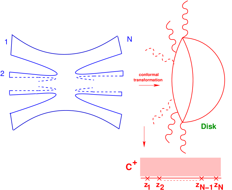
Figure 3: World–sheet describing the scattering of $N$ open strings.

Asymptotic scattering of strings yields the string $S$–matrix defined by the emission and absorption of strings at space–time infinity, i.e. the open strings are incoming and outgoing at infinity. In this case the world–sheet can conformally be mapped to the half–sphere with the emission and absorption of strings taking place at the boundary through some vertex operators. Source boundaries representing the emission and absorption of strings at infinity become points accounting for the vertex operator insertions along the boundary of the half–sphere (disk). After projection onto the upper half plane ${\bf C}^{+}$ the strings are created at the $N$ positions $z_{i},\ i=1,\ldots,N$ along the (compactified) real axis ${\bf R}{\bf P}^{1}$. By this there appears a natural ordering $\Pi\in S_{N}$ of open string vertex operator insertions $z_{i}$ along the boundary of the disk given by $z_{\Pi(1)}<\ldots<z_{\Pi(N)}$. To conclude, the topology of the string world–sheet describing tree–level scattering of open strings is a disk or upper half plane ${\bf C}^{+}$. On the other hand, the tree–level scattering of closed strings is characterized by a complex sphere ${\bf P}^{1}$ with vertex operator insertions on it.

At the $N$ positions $z_{i}$ massless strings carrying the external four–momenta $k_{i},\ i=1,\ldots,N$ and other quantum numbers are created, subject to momentum conservation $k_{1}+\ldots+k_{N}=0$. Due to conformal invariance one has to integrate over all vertex operator positions $z_{i}$ in any amplitude computation. Therefore, for a given ordering $\Pi$ open string amplitudes ${\cal A}^{o}(\Pi)$ are expressed by integrals along the boundary of the world–sheet disk (real projective line) as iterated (real) integrals on ${\bf R}{\bf P}^{1}$ giving rise to multi–dimensional integrals on the space ${\cal M}_{0,N}({\bf R})$ defined in (2.4). The $N$ external four–momenta $k_{i}$ constitute the kinematic invariants of the scattering process:

$$s_{ij}=(k_{i}+k_{j})^{2}=2k_{i}k_{j}\ .$$ (6.101)

Out of (6.101) there are $\frac{1}{2}N(N-3)$ independent kinematic invariants involving $N$ external momenta $k_{i},\ i=1,\ldots,N$. Any amplitude analytically depends on those independent kinematic invariants $s_{ij}$.

A priori there are $N!$ orderings $\Pi$ of the vertex operator positions $z_{i}$ along the boundary. However, string world–sheet symmetries like cyclicity, reflection and parity give relations between different orderings. In fact, by using monodromy properties on the world–sheet further relations are found and any superstring amplitude ${\cal A}^{o}(\Pi)$ of a given ordering $\Pi$ can be expressed in terms of a minimal basis of $(N-3)!$ amplitudes Stieberger:2009hq ; Vanhove :

$${\cal A}^{o}(\sigma):={\cal A}^{o}(1,\sigma(2,\ldots,N-2),N-1,N)\ \ \ ,\ \ \ \sigma\in S_{N-3}\ .$$ (6.102)

The amplitudes (6.102) are functions of the string tension $\alpha^{\prime}$. Power series expansion in $\alpha^{\prime}$ yields iterated integrals (3.20) multiplied by some polynomials in the parameters (6.101).

On the other hand, closed string amplitudes are given by integrals over the complex world–sheet sphere ${\bf P}^{1}$ as iterated integrals integrated independently on all choices of paths. While in the $\alpha^{\prime}$–expansion of open superstring tree–level amplitudes generically the whole space of MZVs (3.36) enters OprisaWU ; GRAV ; SS , closed superstring tree–level amplitudes exhibit only a subset of MZVs appearing in their $\alpha^{\prime}$–expansion GRAV ; SS . This subclass can be identified StiebergerWEA as the single–valued multiple zeta values (SVMZVs) (4.63).

The open superstring $N$–gluon tree–level amplitude ${\mathfrak{A}}^{o}_{N}$ in type I superstring theory decomposes into a sum

$${\mathfrak{A}}^{o}_{N}=(g_{YM}^{o})^{N-2}\ \sum_{\Pi\in S_{N}/{\bf Z}_{2}}{\rm Tr}(T^{a_{\Pi(1)}}\ldots T^{a_{\Pi(N)}})\ {\cal A}^{o}(\Pi(1),\ldots,\Pi(N))$$ (6.103)

over color ordered subamplitudes ${\cal A}^{o}(\Pi(1),\ldots,\Pi(N))$ supplemented by a group trace over matrices $T^{a}$ in the fundamental representation. Above, the YM coupling is denoted by $g_{YM}^{o}$, which in type I superstring theory is given by $g_{YM}^{o}\sim e^{\Phi/2}$ with the dilaton field $\Phi$. The sum runs over all permutations $S_{N}$ of labels $i=1,\ldots,N$ modulo cyclic permutations ${\bf Z}_{2}$, which preserve the group trace. The $\alpha^{\prime}\rightarrow 0$ limit of the open superstring amplitude (6.103) matches the $N$–gluon scattering amplitude of super Yang–Mills (SYM):

$$\left.{\cal A}^{o}(\Pi(1),\ldots,\Pi(N))\right|_{\alpha^{\prime}=0}=A(\Pi(1),\ldots,\Pi(N))\ .$$ (6.104)

As a consequence from (6.102) also in SYM one has a minimal basis of $(N-3)!$ independent partial subamplitudes Bern:2008qj :

$$A(\sigma):=A(1,\sigma(2,\ldots,N-2),N-1,N)\ \ \ ,\ \ \ \sigma\in S_{N-3}\ .$$ (6.105)

Hence, for the open superstring amplitude we may consider a vector ${\cal A}^{o}$ with its entries ${\cal A}^{o}_{\sigma}={\cal A}^{o}(\sigma)$ describing the $(N-3)!$ independent open $N$–point superstring subamplitudes (6.102), while for SYM we have another vector $A$ with entries $A_{\sigma}=A(\sigma)$:

$${\cal A}^{o} = (N-3)!\ \mbox{dimensional vector encompassing}$$

$$\mbox{\hskip 28.45274pt{\bf all} independent superstring subamplitudes}\ {\cal A}^{o}_{\sigma}={\cal A}^{o}(\sigma),\ \sigma\in S_{N-3}\ ,$$

$$A = (N-3)!\ \mbox{dimensional vector encompassing}$$

$$\mbox{\hskip 28.45274pt{\bf all} independent SYM subamplitudes}\ A_{\sigma}=A(\sigma),\ \sigma\in S_{N-3}\ .$$

The two linear independent $(N-3)!$–dimensional vectors ${\cal A}$ and $A$ are related by a non–singular matrix of rank $(N-3)!$. An educated guess is the following relation

$${\cal A}^{o}=F\ A\ ,$$ (6.106)

with the period matrix $F$ given in (3.29). Note, that with (3.30) the Ansatz (6.106) matches the condition (6.104). In components the relation (6.106) reads:

$${\cal A}^{o}(\pi)=\sum_{\sigma\in S_{N-3}}F_{\pi\sigma}\ A(\sigma)\ \ \ ,\ \ \ \pi\in S_{N-3}\ .$$ (6.107)

In fact, an explicit string computation proves the relation (6.106) MafraNV ; MafraNW .

Let us now move on to the scattering of closed strings. In heterotic string vacua gluons are described by massless closed strings. Therefore, we shall consider the closed superstring $N$–gluon tree–level amplitude ${\mathfrak{A}}_{N}^{c}$ in heterotic superstring theory. The string world–sheet describing the tree–level scattering of $N$ closed strings has the topology of a complex sphere with $N$ insertions of vertex operators. The closed string has holomorphic and anti–holomorphic fields. The anti–holomorphic part is similar to the open string case and describes the space–time (or superstring) part. On the other hand, the holomorphic part accounts for the gauge degrees of freedom through current insertions on the world–sheet. As in the open string case (6.103), the single trace part decomposes into the sum

$${\mathfrak{A}}_{N,\;{\rm s.t.}}^{c}=(g_{YM}^{\rm HET})^{N-2}\ \sum_{\Pi\in S_{N}/{\bf Z}_{2}}{\rm tr}(T^{a_{\Pi(1)}}\ldots T^{a_{\Pi(N)}})\ {\cal A}^{c}(\Pi(1),\ldots,\Pi(N))$$ (6.108)

over partial subamplitudes ${\cal A}^{c}(\Pi)$ times a group trace over matrices $T^{a}$ in the vector representation. In the $\alpha^{\prime}\rightarrow 0$ limit the latter match the $N$–gluon scattering subamplitudes of SYM

$$\left.{\cal A}^{c}(\Pi(1),\ldots,\Pi(N))\right|_{\alpha^{\prime}=0}=A(\Pi(1),\ldots,\Pi(N))\ ,$$ (6.109)

similarly to open string case (6.104). Again, the partial subamplitudes ${\cal A}^{c}(\Pi)$ can be expressed in terms of a minimal basis of $(N-3)!$ elements ${\cal A}^{c}(\rho),\ \rho\in S_{N-3}$. The latter have been computed in Stieberger:2014hba and are given by

$${\cal A}^{c}(\rho)=(-1)^{N-3}\ \sum_{\sigma\in S_{N-3}}\sum_{\overline{\rho}\in S_{N-3}}J[\rho\,|\,\overline{\rho}]\ S[\overline{\rho}|\sigma]\ A(\sigma)\ ,\ \ \rho\in S_{N-3}\ ,$$ (6.110)

with the complex sphere integral

$$J[\rho\,|\,\overline{\rho}] := V_{\rm CKG}^{-1}\ \left(\prod_{j=1}^{N}\int\limits_{z_{j}\in{\bf C}}d^{2}z_{j}\right)\ \prod\limits_{i<j}^{N}|z_{ij}|^{2\alpha^{\prime}s_{ij}}\ \frac{1}{z_{1\rho(2)}z_{\rho(2),\rho(3)}\ldots z_{\rho(N-2),N-1}z_{N-1,N}z_{N,1}}$$ (6.111)

$$\times \displaystyle{\frac{1}{\overline{z}_{1\overline{\rho}(2)}\overline{z}_{\overline{\rho}(2),\overline{\rho}(3)}\ldots\overline{z}_{\overline{\rho}(N-3),\overline{\rho}(N-2)}\overline{z}_{\overline{\rho}(N-2),N}\overline{z}_{N,N-1}\ \overline{z}_{N-1,1}}}\ ,$$ (6.112)

the kernel $S$ introduced in (3.28) and the SYM amplitudes (6.105). In (6.112) the rational function comprising the dependence on holomorphic and anti–holomorphic vertex operator positions shows some pattern depicted in Fig. 4.

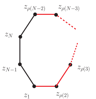
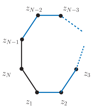
Figure 4: $N$–gons describing the cyclic structures of holomorphic and anti–holomorphic cell forms.

Based on the results StiebergerWEA the following (matrix) identity has been established in Stieberger:2014hba

$$J={\rm sv}(Z)\ ,$$ (6.113)

relating the complex integral (6.112) to the real iterated integral (3). The holomorphic part of (6.112) simply turns into the corresponding integral ordering of (3). As a consequence of (6.113) we find the following relation between the closed (6.110) and open (6.107) superstring gluon amplitude Stieberger:2014hba :

$${\cal A}^{c}(\rho)={\rm sv}\left({\cal A}^{o}(\rho)\right)\ \ \ ,\ \ \ \rho\in S_{N-3}\ .$$ (6.114)

To conclude, the single trace heterotic gauge amplitudes ${\cal A}^{c}(\rho)$ referring to the color ordering $\rho$ are simply obtained from the relevant open string gauge amplitudes ${\cal A}^{o}(\rho)$ by imposing the projection ${\rm sv}$ introduced in (4.77). Therefore, the $\alpha^{\prime}$–expansion of the heterotic amplitude ${\cal A}^{c}(\rho)$ can be obtained from that of the open superstring amplitude ${\cal A}^{o}(\rho)$ by simply replacing MZVs by their corresponding SVMZVs according to the rules introduced in (4.77). The relation (6.114) between the heterotic gauge amplitude ${\cal A}^{c}$ and the type I gauge amplitude $A^{o}$ establishes a non–trivial relation between closed string and open string amplitudes: the $\alpha^{\prime}$–expansion of the closed superstring amplitude can be cast into the same algebraic form as the open superstring amplitude: the closed superstring amplitude is essentially the single–valued (sv) version of the open superstring amplitude.

Also closed string amplitudes other than the heterotic (single–trace) gauge amplitudes (6.110) can be expressed as single–valued image of some open string amplitudes. From (6.113) the closed string analog of (3.27) follows:

$$\left.J\right|_{\alpha^{\prime}=0}=(-1)^{N-3}\ S^{-1}\ .$$ (6.115)

Hence, the set of complex world–sheet sphere integrals (6.112) are the closed string analogs of the open string world–sheet disk integrals (3) and serve as building blocks to construct any closed string amplitude. After applying partial integrations to remove double poles, which are responsible for spurious tachyonic poles, further performing partial fraction decompositions and partial integration relations all closed superstring amplitudes can be expressed in terms of the basis (6.112), which in turn through (6.113) can be related to the basis of open string amplitudes (3). As a consequence the $\alpha^{\prime}$–dependence of any closed string amplitude is given by that of the underlying open string amplitudes. This non–trivial connection between open and closed string amplitudes at the string tree–level points into a deeper connection between gauge and gravity amplitudes than what is implied by Kawai–Lewellen–Tye relations KawaiXQ .

7 Complex vs. iterated integrals

Perturbative open and closed string amplitudes seem to be rather different due to their underlying different world–sheet topologies with or without boundaries, respectively. On the other hand, mathematical methods entering their computations reveal some unexpected connections. As we have seen in the previous section a new relation (6.113) between open (3) and closed (6.112) string world–sheet integrals holds.

Open string world–sheet disk integrals (3) are described as real iterated integrals on the space ${\cal M}_{0,N}({\bf R})$ defined in (2.4), while closed string world–sheet sphere integrals (6.112) are given by integrals on the space ${\cal M}_{0,N}({\bf C})$ defined in (2.3). The latter integrals, which can be considered as iterated integrals on ${\bf P}^{1}$ integrated independently on all choices of paths, are more involved than the real iterated integrals appearing in open string amplitudes. The observation (6.113) that complex integrals can be expressed as real iterated integrals subject to the projection ${\rm sv}$ has exhibited non–trivial relations between open and closed string amplitudes (6.114). In this section we shall elaborate on these connections at the level of the world–sheet integrals.

The simplest example of (6.113) arises for $N=4$ yielding the relation

$$\int_{\bf C}d^{2}z\ \frac{|z|^{2s}\ |1-z|^{2u}}{z\ (1-z)\ \overline{z}}={\rm sv}\left(\int_{0}^{1}dx\ x^{s-1}\ (1-x)^{u}\right)\ ,$$ (7.116)

with $s,u\in{\bf R}$ such that both integrals converge. While the integral on the l.h.s. of (7.116) describes a four–point closed string amplitude the integral on the r.h.s. describes a four–point open string amplitude. Hence, the meaning of (7.116) w.r.t. to the corresponding closed vs. open string world–sheet diagram describing four–point scattering (6.114) can be depicted as Fig. 5.

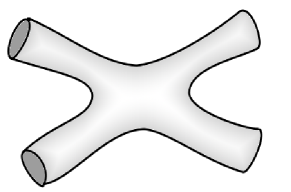
Figure 5: Relation between closed and open string world–sheet diagram describing four–point scattering.

= sv

After performing the integrations the relation (7.116) becomes (with $s+t+u=0$):

$$\frac{\Gamma(s)\ \Gamma(u)\ \Gamma(t)}{\Gamma(-s)\ \Gamma(-u)\ \Gamma(-t)}={\rm sv}\left(\frac{\Gamma(1+s)\ \Gamma(1+u)}{\Gamma(1+s+u)}\right)\ .$$ (7.117)

Essentially, this equality (when acting on $[e_{0},e_{1}]$) represents the relation between the Deligne (4.67) and Drinfeld (4.45) associators in the explicit representation of the limit ${\rm mod}(g^{\prime})^{2}$ with $(g^{\prime})^{2}=[g,g]^{2}$, $s=-{\rm ad}_{e_{1}},\ u={{\rm ad}}_{e_{0}}$ and ${\rm ad}_{x}y=[x,y]$, i.e. dropping all quadratic commutator terms Drummond:2013vz ; StiebergerWEA . Note, that applying Kawai–Lewellen–Tye (KLT) relations KawaiXQ to the complex integral of (7.116) rather yields

$$\int_{\bf C}d^{2}z\ \frac{|z|^{2s}\ |1-z|^{2u}}{z\ (1-z)\ \overline{z}}=\sin(\pi u)\ \left(\int_{0}^{1}dx\ x^{s-1}\ (1-x)^{u-1}\right)\ \left(\int_{1}^{\infty}dx\ x^{t-1}\ (1-x)^{u}\right)\ ,$$ (7.118)

expressing the latter in terms of a square of real iterated integrals instead of a single real iterated integral as in (7.116). In fact, any direct computation of this complex integral by means of a Mellin representation or Gegenbauer decomposition ends up at (7.118).

Similar (7.116) explicit and direct correspondences (6.113) between the complex sphere integrals $J$ and the real disk integrals $Z$ can be made for $N\geq 5$. In order to familiarize with the matrix notation let us explicitly write the case (6.113) for $N=5$ (with (2.1)):

$$\hskip-35.56593pt\left(\begin{array}[]{lcl}\displaystyle{\int\limits_{z_{2},z_{3}\in{\bf C}}d^{2}z_{2}\ d^{2}z_{3}\ \frac{\prod\limits_{i<j}^{4}|z_{ij}|^{2\alpha^{\prime}s_{ij}}}{z_{12}z_{23}z_{34}\ \overline{z}_{12}\overline{z}_{23}}}&\displaystyle{\int\limits_{z_{2},z_{3}\in{\bf C}}d^{2}z_{2}\ d^{2}z_{3}\ \frac{\prod\limits_{i<j}^{4}|z_{ij}|^{2\alpha^{\prime}s_{ij}}}{z_{12}z_{23}z_{34}\ \overline{z}_{13}\overline{z}_{32}}}\\ \displaystyle{\int\limits_{z_{2},z_{3}\in{\bf C}}d^{2}z_{2}\ d^{2}z_{3}\ \frac{\prod\limits_{i<j}^{4}|z_{ij}|^{2\alpha^{\prime}s_{ij}}}{z_{13}z_{32}z_{24}\ \overline{z}_{12}\overline{z}_{23}}}&\displaystyle{\int\limits_{z_{2},z_{3}\in{\bf C}}d^{2}z_{2}\ d^{2}z_{3}\ \frac{\prod\limits_{i<j}^{4}|z_{ij}|^{2\alpha^{\prime}s_{ij}}}{z_{13}z_{32}z_{24}\ \overline{z}_{13}\overline{z}_{32}}}\end{array}\right)$$ (7.121)

$$\hskip 7.11317pt={\rm sv}\left(\begin{array}[]{lcl}\displaystyle{\int\limits_{0<z_{2}<z_{3}<1}dz_{2}\ dz_{3}\ \frac{\prod\limits_{i<j}^{4}|z_{ij}|^{\alpha^{\prime}s_{ij}}}{z_{12}z_{23}}}&\displaystyle{\int\limits_{0<z_{2}<z_{3}<1}dz_{2}\ dz_{3}\ \frac{\prod\limits_{i<j}^{4}|z_{ij}|^{\alpha^{\prime}s_{ij}}}{z_{13}z_{32}}}\\ \displaystyle{\int\limits_{0<z_{3}<z_{2}<1}dz_{2}\ dz_{3}\ \frac{\prod\limits_{i<j}^{4}|z_{ij}|^{\alpha^{\prime}s_{ij}}}{z_{12}z_{23}}}&\displaystyle{\int\limits_{0<z_{3}<z_{2}<1}dz_{2}\ dz_{3}\ \frac{\prod\limits_{i<j}^{4}|z_{ij}|^{\alpha^{\prime}s_{ij}}}{z_{13}z_{32}}}\end{array}\right)$$ (7.124)

In (7.124) we explicitly see how the presence of the holomorphic gauge insertion in the complex integrals results in the projection onto real integrals involving only the right–moving part. Similar matrix relations can be extracted from (6.113) beyond $N>5$.

From (6.113) it follows that the $\alpha^{\prime}$–expansion of the closed string amplitude can be obtained from that of the open superstring amplitude by simply replacing MZVs by their corresponding SVMZVs according to the rules introduced in (4.77). Hence, closed string amplitudes use only the smaller subspace of SVMZVs. From a physical point of view SVMZVs appear in the computation of graphical functions (positive functions on the punctured complex plane) for certain Feynman amplitudes Schnetz . In supersymmetric Yang–Mills theory a large class of Feynman integrals in four space–time dimensions lives in the subspace of SVMZVs or SVMPs. As pointed out by Brown in SVMZV , this fact opens the interesting possibility to replace general amplitudes with their single–valued versions (defined in (4.77) by the map ${\rm sv}$), which should lead to considerable simplifications. In string theory this simplification occurs by replacing open superstring amplitudes by their single–valued versions describing closed superstring amplitudes.

Acknowledgments

We wish to thank the organizers (especially José Burgos, Kurush Ebrahimi-Fard, and Herbert Gangl) of the workshop Research Trimester on Multiple Zeta Values, Multiple Polylogarithms, and Quantum Field Theory and the conference Multiple Zeta Values, Modular Forms and Elliptic Motives II at ICMAT, Madrid for inviting me to present the work exhibited in this publication and creating a stimulating atmosphere.

References

- (1) N. Arkani-Hamed, J.L. Bourjaily, F. Cachazo, A.B. Goncharov, A. Postnikov and J. Trnka, “Scattering Amplitudes and the Positive Grassmannian,” [arXiv:1212.5605 [hep-th]].
- (2) N. Arkani-Hamed and J. Trnka, “The Amplituhedron,” JHEP 1410, 30 (2014). [arXiv:1312.2007 [hep-th]].
- (3) Z. Bern, L.J. Dixon, M. Perelstein and J.S. Rozowsky, “Multileg one loop gravity amplitudes from gauge theory,” Nucl. Phys. B 546, 423 (1999). [hep-th/9811140].
- (4) Z. Bern, J.J.M. Carrasco and H. Johansson, “New Relations for Gauge-Theory Amplitudes,” Phys. Rev. D 78, 085011 (2008) [arXiv:0805.3993 [hep-ph]].
- (5) F. Beukers, “Algebraic A–hypergeometric functions,” Invent. Math. 180 (2010), 589–610.
- (6) N.E.J. Bjerrum-Bohr, P.H. Damgaard and P. Vanhove, “Minimal Basis for Gauge Theory Amplitudes,” Phys. Rev. Lett. 103, 161602 (2009) [arXiv:0907.1425 [hep-th]].
- (7) N.E.J. Bjerrum-Bohr, P.H. Damgaard, T. Sondergaard and P. Vanhove, “The Momentum Kernel of Gauge and Gravity Theories,” JHEP 1101, 001 (2011). [arXiv:1010.3933 [hep-th]].
- (8) J. Blümlein, D.J. Broadhurst and J.A.M. Vermaseren, “The Multiple Zeta Value Data Mine,” Comput. Phys. Commun. 181, 582 (2010). [arXiv:0907.2557 [math-ph]].
- (9) R.H. Boels, “On the field theory expansion of superstring five point amplitudes,” Nucl. Phys. B 876, 215 (2013) [arXiv:1304.7918 [hep-th]].
- (10) C. Bogner and S. Weinzierl, “Periods and Feynman integrals,” J. Math. Phys. 50, 042302 (2009). [arXiv:0711.4863 [hep-th]].
- (11) D.J. Broadhurst and D. Kreimer, “Association of multiple zeta values with positive knots via Feynman diagrams up to 9 loops,” Phys. Lett. B 393, 403 (1997). [hep-th/9609128].
- (12) J. Broedel, O. Schlotterer and S. Stieberger, “Polylogarithms, Multiple Zeta Values and Superstring Amplitudes,” Fortsch. Phys. 61, 812 (2013). [arXiv:1304.7267 [hep-th]].
- (13) J. Broedel, O. Schlotterer, S. Stieberger and T. Terasoma, “Notes on Lie Algebra structure of Superstring Amplitudes,” unpublished.
- (14) F. Brown, “Single-valued multiple polylogarithms in one variable,” C.R. Acad. Sci. Paris, Ser. I 338, 527-532 (2004).
- (15) F. Brown, “Multiple zeta values and periods of moduli spaces ,” Ann. Sci. Ec. Norm. Sup. 42, 371 (2009). [arXiv:math/0606419 [math.AG]].
- (16) F.C.S. Brown, S. Carr, and L. Schneps, “Algebra of cell-zeta values,” Compositio Math. 146 (2010), 731-771
- (17) F. Brown, “On the decomposition of motivic multiple zeta values,” in ‘Galois-Teichmüller Theory and Arithmetic Geometry’, Advanced Studies in Pure Mathematics 63 (2012) 31-58 [arXiv:1102.1310 [math.NT]].
- (18) F.C.S. Brown and A. Levin, “Multiple Elliptic Polylogarithms,” [arXiv:1110.6917 [math.NT]].
- (19) F. Brown, “Mixed Tate Motives over ,” Ann. Math. 175 (2012) 949–976.
- (20) F. Brown, “Single-valued Motivic Periods and Multiple Zeta Values,” SIGMA 2, e25 (2014) [arXiv:1309.5309 [math.NT]].
- (21) F. Brown, “Periods and Feynman amplitudes,” arXiv:1512.09265 [math-ph].
- (22) F. Brown, “A class of non-holomorphic modular forms I,” arXiv:1707.01230 [math.NT].
- (23) P. Deligne, “Le groupe fondamental de la droite projective moins trois points,” in: Galois groups over , Springer, MSRI publications 16 (1989), 72-297; “Periods for the fundamental group,” Arizona Winter School 2002.
- (24) V.G. Drinfeld, “On quasitriangular quasi-Hopf algebras and on a group that is closely connected with ,” Alg. Anal. 2, 149 (1990); English translation: Leningrad Math. J. 2 (1991), 829-860.
- (25) J.M. Drummond and E. Ragoucy, “Superstring amplitudes and the associator,” JHEP 1308, 135 (2013) [arXiv:1301.0794 [hep-th]].
- (26) I.M. Gelfand, M.M. Kapranov, A.V. Zelevinsky, “Generalized Euler integrals and –hypergeometric functions,” Adv. Math. 84 (1990) 255–271.
- (27) J. Golden, A.B. Goncharov, M. Spradlin, C. Vergu and A. Volovich, “Motivic Amplitudes and Cluster Coordinates,” JHEP 1401, 091 (2014). [arXiv:1305.1617 [hep-th]].
- (28) A.B. Goncharov, “Multiple zeta-values, Galois groups, and geometry of modular varieties”, arXiv:math/0005069v2 [math.AG].
- (29) A.B. Goncharov, “Multiple polylogarithms and mixed Tate motives,” [arXiv:math/ 0103059v4 [math.AG]].
- (30) A. Goncharov and Y. Manin, “Multiple –motives and moduli spaces ”, Compos. Math. 140 (2004) 1–14 [arXiv:math/0204102].
- (31) A.B. Goncharov, “Galois symmetries of fundamental groupoids and noncommutative geometry,” Duke Math. J. 128 (2005) 209-284. [arXiv:math/0208144v4 [math.AG]].
- (32) A.B. Goncharov, private communication.
- (33) Y. Ihara, “Some arithmetic aspects of Galois actions in the pro-p fundamental group of ,” in Arithmetic Fundamental Groups and Noncommutative Algebra, Proceedings of Symposia in Pure Mathematics, Vol 70 (2002).
- (34) H. Kawai, D.C. Lewellen and S.H.H. Tye, “A Relation Between Tree Amplitudes Of Closed And Open Strings,” Nucl. Phys. B 269, 1 (1986).
- (35) M. Kontsevich and D. Zagier, “Periods,” in: B. Engquist, and W. Schmid, Mathematics unlimited – 2001 and beyond, Berlin, New York: Springer-Verlag, 771–808.
- (36) T.Q.T. Le and J. Murakami, “Kontsevich’s integral for the Kauffman polynomial,” Nagoya Math. J. 142 (1996), 39-65.
- (37) C.R. Mafra, O. Schlotterer and S. Stieberger, “Complete N-Point Superstring Disk Amplitude I. Pure Spinor Computation,” Nucl. Phys. B 873, 419 (2013). [arXiv:1106.2645 [hep-th]];
- (38) C.R. Mafra, O. Schlotterer and S. Stieberger, “Complete N-Point Superstring Disk Amplitude II. Amplitude and Hypergeometric Function Structure,” Nucl. Phys. B 873, 461 (2013). [arXiv:1106.2646 [hep-th]].
- (39) D. Oprisa and S. Stieberger, “Six gluon open superstring disk amplitude, multiple hypergeometric series and Euler-Zagier sums,” [hep-th/0509042].
- (40) G. Puhlfürst and S. Stieberger, “Differential Equations, Associators, and Recurrences for Amplitudes,” Nucl. Phys. B 902, 186 (2016) [arXiv:1507.01582 [hep-th]]; “A Feynman Integral and its Recurrences and Associators,” Nucl. Phys. B 906, 168 (2016) [arXiv:1511.03630 [hep-th]].
- (41) O. Schlotterer and S. Stieberger, “Motivic Multiple Zeta Values and Superstring Amplitudes,” J. Phys. A 46, 475401 (2013). [arXiv:1205.1516 [hep-th]].
- (42) O. Schnetz, “Graphical functions and single-valued multiple polylogarithms,” Commun. Num. Theor. Phys. 08 (2014) 589 [arXiv:1302.6445 [math.NT]].
- (43) S. Stieberger and T.R. Taylor, “Multi-Gluon Scattering in Open Superstring Theory,” Phys. Rev. D 74, 126007 (2006). [hep-th/0609175].
- (44) S. Stieberger, “Open & Closed vs. Pure Open String Disk Amplitudes,” arXiv:0907.2211 [hep-th].
- (45) S. Stieberger, “Constraints on Tree-Level Higher Order Gravitational Couplings in Superstring Theory,” Phys. Rev. Lett. 106, 111601 (2011) [arXiv:0910.0180 [hep-th]].
- (46) S. Stieberger, “Closed superstring amplitudes, single-valued multiple zeta values and the Deligne associator,” J. Phys. A 47, 155401 (2014). [arXiv:1310.3259 [hep-th]].
- (47) S. Stieberger and T.R. Taylor, “Closed String Amplitudes as Single-Valued Open String Amplitudes,” Nucl. Phys. B 881, 269 (2014) [arXiv:1401.1218 [hep-th]].
- (48) T. Terasoma, “Selberg Integrals and Multiple Zeta Values”, Compos. Math. 133 1–24, 2002.
- (49) H. Tsunogai, “On ranks of the stable derivation algebra and Deligne’s problem,” Proc. Japan Acad. Ser. A, 73 (1997) 29-31.
- (50) D. Zagier, “Values of zeta functions and their applications,” in First European Congress of Mathematics (Paris, 1992), Vol. II, A. Joseph et. al. (eds.), Birkhäuser, Basel, 1994, pp. 497-512.