Parallel Equivalence Class Sorting: Algorithms, Lower Bounds, and Distribution-Based Analysis

Abstract

We study parallel comparison-based algorithms for finding all equivalence classes of a set of $n$ elements, where sorting according to some total order is not possible. Such scenarios arise, for example, in applications, such as in distributed computer security, where each of $n$ agents are working to identify the private group to which they belong, with the only operation available to them being a zero-knowledge pairwise-comparison (which is sometimes called a “secret handshake”) that reveals only whether two agents are in the same group or in different groups. We provide new parallel algorithms for this problem, as well as new lower bounds and distribution-based analysis.

1 Introduction

In the Equivalence Class Sorting problem, we are given a set, $S$, of $n$ elements and an equivalence relation, and we are asked to group the elements of the set into their equivalence classes by only making pairwise equivalence tests (e.g., see [12]). For example, imagine a convention of $n$ political interns where each person at the convention belongs to one of $k$ political parties, such as Republican, Democrat, Green, Labor, Libertarian, etc., but no intern wants to openly express his or her party affiliation unless they know they are talking with someone of their same party. Suppose further that each party has a secret handshake that two people can perform that allows them to determine whether they are in the same political party (or they belong to different unidentified parties). We are interested in this paper in the computational complexity of the equivalence class sorting problem in distributed and parallel settings, where we would like to minimize the total number of parallel comparison rounds and/or the total number of comparisons needed in order to classify every element in $S$.

An important property of the equivalence class sorting problem is that it is not possible to order the elements in $S$ according to some total ordering that is consistent with the equivalence classes. Such a restriction could come from a general lack of such an ordering or from security or privacy concerns. For example, consider the following applications:

• Generalized fault diagnosis. Suppose that each of $n$ different computers are in one of $k$ distinct malware states, depending on whether they have been infected with various computer worms. Each worm does not wish to reveal its presence, but it nevertheless has an ability to detect when another computer is already infected with it (or risk autodetection by an exponential cascade, as occurred with the Morris worm [15]). But a worm on one computer is unlikely to be able to detect a different kind of worm on another computer. Thus, two computers can only compare each other to determine if they have exactly the same kinds of infections or not. The generalized fault diagnosis problem, therefore, is to have the $n$ computers classify themselves into $k$ malware groups depending on their infections, where the only testing method available is for two computers to perform a pairwise comparison that tells them that they are either in the same malware state or they are in different states. This is a generalization of the classic fault diagnosis problem, where there are only two states, “faulty” or “good,” which is studied in a number of interesting papers, including one from the very first SPAA conference (e.g., see [5, 6, 4, 10, 17, 18]).

• Group classification via secret handshakes. This is a cryptographic analogue to the motivating example given above of interns at a political convention. In this case, $n$ agents are each assigned to one of $k$ groups, such that any two agents can perform a cryptographic “secret handshake” protocol that results in them learning only whether they belong to the same group or not (e.g., see [7, 11, 20, 22]). The problem is to perform an efficient number of pairwise secret-handshake tests in a few parallel rounds so that each agent identifies itself with the others of its group.

• Graph mining. Graph mining is the study of structure in collections of graphs [8]. One of the algorithmic problems in this area is to classify which of a collection of $n$ graphs are isomorphic to one another (e.g., see [16]). That is, testing if two graphs are in the same group involves performing a graph isomorphism comparison of the two graphs, which is a computation that tends to be nontrivial but is nevertheless computationally feasible in some contexts (e.g., see [3]).

Note that each of these applications contains two important features that form the essence of the equivalence class sorting problem:

1. In each application, it is not possible to sort elements according to a known total order, either because no such total order exists or because it would break a security/privacy condition to provide such a total order.

2. The equivalence or nonequivalence between two elements can be determined only through pairwise comparisons.

There are nevertheless some interesting differences between these applications, as well, which motivate our study of two different versions of the equivalence class sorting problem. Namely, in the first two applications, the comparisons done in any given round in an algorithm must be disjoint, since the elements themselves are performing the comparisons. In the latter two applications, however, the elements are the objects of the comparisons, and we could, in principle, allow for comparisons involving multiple copies of the same element in each round. For this reason, we allow for two versions of the equivalence class sorting problem:

• Exclusive-Read (ER) version. In this version, each element in $S$ can be involved in at most a single comparison of itself and another element in $S$ in any given comparison round.

• Concurrent-Read (CR) version. In this version, each element in $S$ can be involved in multiple comparisons of itself and other elements in $S$ in any comparison round.

In either version, we are interested in minimizing the number of parallel comparison rounds and/or the total number of comparisons needed to classify every element of $S$ into its group.

Because we expect the number parallel comparison rounds and the total number of comparisons to be the main performance bottlenecks, we are interested here in studying the equivalence class sorting problem in Valiant’s parallel comparison model [21], which only counts steps in which comparisons are made. This is a synchronous computation model that does not count any steps done between comparison steps, for example, to aggregate groups of equivalent elements based on comparisons done in previous steps.

1.1 Related Prior Work

In addition to the references cited above that motivate the equivalence class sorting problem or study the special case when the number of groups, $k$, is two, Jayapaul et al. [12] study the general equivalence class sorting problem, albeit strictly from a sequential perspective. For example, they show that one can solve the equivalence class sorting problem using $O(n^{2}/\ell)$ comparisons, where $\ell$ is the size of the smallest equivalence class. They also show that this problem has a lower bound of $\Omega(n^{2}/\ell^{2})$ even if the value of $\ell$ is known in advance.

The equivalence class sorting problem is, of course, related to comparison-based algorithms for computing the majority or mode of a set of elements, for which there is an extensive set of prior research (e.g., see [2, 1, 9, 19]). None of these algorithms for majority or mode result in efficient parallel algorithms for the equivalence class sorting problem, however.

1.2 Our Results

In this paper, we study the equivalence class sorting (ECS) problem from a parallel perspective, providing a number of new results, including the following:

1. The CR version of the ECS problem can be solved in $O(k+\log\log n)$ parallel rounds using $n$ processors, were $k$ is the number of equivalence classes.

2. The ER version of the ECS problem can be solved in $O(k\log n)$ parallel rounds using $n$ processors, were $k$ is the number of equivalence classes.

3. The ER version of the ECS problem can be solved in $O(1)$ parallel rounds using $n$ processors, for the case when $\ell$ is at least $\lambda n$, for a fixed constant $0<\lambda\leq 0.4$, where $\ell$ is the size of the smallest equivalence class.

4. If every equivalence class is of size $f$, then solving the ECS problem requires $\Omega(n^{2}/f)$ total comparisons. This improves a lower bound of $\Omega(n^{2}/f^{2})$ by Jayapaul et al. [12].

5. Solving the ECS problem requires $\Omega(n^{2}/\ell)$ total comparisons, where $\ell$ is the size of the smallest equivalence class. This improves a lower bound of $\Omega(n^{2}/\ell^{2})$ by Jayapaul et al. [12].

6. In Section 4, we study how to efficiently solve the ECS problem when the input is drawn from a known distribution on equivalence classes. In this setting, we assume $n$ elements have been sampled and fed as input to the algorithm. We establish a relationship between the mean of the distribution and the algorithm’s total number of comparisons, obtaining upper bounds with high probability for a variety of interesting distributions.

7. We provide the results of several experiments to validate the results from Section 4 and study how total comparison counts change as parameters of the distributions change.

Our methods are based on several novel techniques, including a two-phased compounding-comparison technique for the parallel upper bounds and the use of a new coloring argument for the lower bounds.

2 Parallel Algorithms

In this section, we provide efficient parallel algorithms for solving the equivalence class sorting (ECS) problem in Valiant’s parallel model of computation [21]. We focus on both the exclusive-read (ER) and concurrent-read (CR) versions of the problem, and we assume we have $n$ processors, each of which can be assigned to one equivalence comparison test to perform in a given parallel round. Note, therefore, that any lower bound, $T(n)$, on the total number of comparisons needed to solve the ECS problem (e.g., as given by Jayapaul et al. [12] and as we discuss in Section 3), immediately implies a lower bound of $\Omega(T(n)/n)$ for the number of parallel rounds of computation using $n$ processors per round. For instance, these lower bounds imply that the number of parallel rounds for solving the ECS problem with $n$ processors must be $\Omega(n/\ell)$ and $\Omega(k)$, respectively, where $k$ is the number of equivalence classes and $\ell$ is the size of the smallest equivalence class.

With respect to upper bounds, recall that Jayapaul et al. [12] studied the ECS problem from a sequential perspective. Unfortunately, their algorithm cannot be easily parallelized, because the comparisons performed in a “round” of their algorithm depend on the results from other comparisons in that same round. Thus, new parallel ECS algorithms are needed.

2.1 Algorithms Based on the Number of Groups

In this subsection, we describe CR and ER algorithms based on knowledge of the number of groups, $k$.

If two sets of elements are sorted into their equivalence classes, merging the two answers into the answer for the union requires at most $k^{2}$ equivalence tests by simply performing a comparison between every pair of equivalence class one from the first answer and one from the second. This idea leads to the following algorithm, which uses a two-phased compounding-comparison technique to solve the ECS problem:

1. Initialize a list of $n$ answers containing the individual input elements.

2. While the number of processors per answer is less than $4k^{2}$, merge pairs of answers by performing $k^{2}$ tests.

3. While there is more than one answer, let $ck^{2}$ be the number of processors available per answer and merge $c$ answers together by performing at most ${c\choose 2}k^{2}$ tests between each of the answers.

We analyze this algorithm in the following two lemmas and we illustrate it in Figure 1.

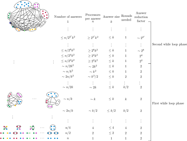
Figure 1: A visualization of the parallel algorithm with a table on the right keeping track of relevant numbers for each loop iteration.

Lemma 1.

The first while loop takes $O(k)$ rounds to complete.

Proof.

In each round the number of equivalence classes in an answer at most doubles until it reaches the upper bound of $k$. In loop iteration $i\leq\lceil\log k\rceil$, the answers are size at most $2^{i}$ and there are $2^{i}$ processors per answer. Therefore it takes at most $2^{i}$ rounds to merge two answers. The number of rounds to reach the $\lceil\log k\rceil$ loop iteration is $O(k)$. For loop iterations $\lceil\log k\rceil<i<\lceil\log k\rceil^{2}$, the answers are size at most $k$, but there are still at most $2^{i}$ processors per answer. The number of rounds needed for these iterations is also $O(k)$, as it forms a geometric sum that adds up to be $O(k)$. This part of the algorithm is illustrated in the bottom half of Figure 1. ∎

Lemma 2.

The second while loop takes $O(\log\log n)$ rounds to complete.

Proof.

When entering the second while, there are more processors per answer than needed to merge just two answers at a time. If an answer has access to $ck^{2}$ processors, then a group of ${c\choose 2}$ answers can merge into one answer in a single round. This means that if there are $n/(ck^{2})$ answers at the start of a round, then we merge groups of $c^{2}/2$ answers into one answer and there are $n/(c^{3}k/2)$ answers remaining. Because $c\geq 4$ by the condition of the first while loop, in the iteration $i$ of the second while loop, there are at most $n/(2^{2^{i}}k)$ answers. And so the second while loop will terminate after $O(\log\log n)$ rounds with the single answer for the entire input. This is illustrated in the top half of Figure 1. ∎

Combining these two lemmas, we get the following.

Theorem 1.

The CR version of the equivalence class sorting problem on $n$ elements and $k$ equivalence classes can be solved in $O(k+\log\log n)$ parallel rounds of equivalence tests, using $n$ processors in Valiant’s parallel comparison model.

Proof.

Lemmas 1 and 2. ∎

We also have the following.

Theorem 2.

The ER version of the equivalence class sorting problem on $n$ elements and $k$ equivalence classes can be solved in $O(k\log n)$ parallel rounds of equivalence tests, using $n$ processors in Valiant’s parallel comparison model.

Proof.

Merging two answers for the ER version of the ECS problem model will always take at most $k$ rounds. Repeatedly merging answers will arrive at one answer in $\log n$ iterations. So equivalence class sorting can be done in $O(k\log n)$ parallel rounds of equivalence tests. ∎

2.2 Algorithms Based on the Smallest Group Size

In this subsection, we describe ER algorithms based on knowledge of $\ell$, the size of the smallest equivalence class. We assume in this section that $\ell\geq\lambda n$, for some constant $\lambda>0$, and we show how to solve the ECS problem in this scenario using $O(1)$ parallel comparison rounds. Our methods are generalizations of previous methods for the parallel fault diagnosis problem when there are only two classes, “good” and “faulty” [5, 6, 4, 10]. Let us assume, therefore, that there are at least 3 equivalence classes.

We begin with a theorem from Goodrich [10].

Theorem 3 (Goodrich [10]).

Let $V$ be a set of $n$ vertices, and let $0<\gamma,\lambda<1$. Let $H_{d}=(V,E)$ be a directed graph defined by the union of $d$ independent randomly-chosen Hamiltonian cycles on $V$ (with all such cycles equally likely). Then, for all subsets $W$ of $V$ of $\lambda n$ vertices, $H_{d}$ induces at least one strongly connected component on $W$ of size greater than $\gamma\lambda n$, with probability at least

$$1-e^{n[(1+\lambda)\ln 2+d(\alpha\ln\alpha+\beta\ln\beta-(1-\lambda)\ln(1-\lambda))]+O(1)},$$

where $\alpha=1-\frac{1-\gamma}{2}\lambda$ and $\beta=1-\frac{1+\gamma}{2}\lambda$.

In the context of the present paper, let us take $\gamma=1/4$, so $\alpha=1-(3/8)\lambda$ and $\beta=1-(5/8)\lambda$. Let us also assume that $\lambda\leq 0.4$, since we are considering the case when the number of equivalence classes is at least $3$; hence, the smallest equivalence class is of size at most $n/3$.

Unfortunately, using standard approximations for the natural logarithm is not sufficient for us to employ the above probability bound for small values of $\lambda$. So instead we use the following inequalities, which hold for $x$ in the range $[0,0.4]$ (e.g., see [13]), and are based on the Taylor series for the natural logarithm:

$$-x-\frac{x^{2}}{2}-\frac{x^{3}}{2}\leq\ln(1-x)\leq-x-\frac{x^{2}}{2}-\frac{x^{3}}{4}.$$

These bounds allow us to bound the main term, $t$, in the above probability of Theorem 3 (for $\gamma=1/4$) as follows:

$$t = \alpha\ln\alpha\ +\ \beta\ln\beta-(1-\lambda)\ln(1-\lambda)$$

$$= (1-\frac{3}{8}\lambda)\ln(1-\frac{3}{8}\lambda)\ +\ (1-\frac{5}{8}\lambda)\ln(1-\frac{5}{8}\lambda)$$

$$-\ (1-\lambda)\ln(1-\lambda)$$

$$\leq (1-\frac{3}{8}\lambda)\left(-\frac{3}{8}\lambda-\frac{1}{2}\left(\frac{3}{8}\lambda\right)^{2}-\frac{1}{4}\left(\frac{3}{8}\lambda\right)^{3}\right)$$

$$+\ (1-\frac{5}{8}\lambda)\left(-\frac{5}{8}\lambda-\frac{1}{2}\left(\frac{5}{8}\lambda\right)^{2}-\frac{1}{4}\left(\frac{5}{8}\lambda\right)^{3}\right)$$

$$-\ (1-\lambda)\left(-\lambda-\frac{\lambda^{2}}{2}-\frac{\lambda^{3}}{2}\right)$$

$$\leq -\frac{3743}{8192}\lambda^{4}+\frac{19}{256}\lambda^{3}-\frac{15}{64}\lambda^{2},$$

which, in turn, is at most

$$-\frac{\lambda^{2}}{8},$$

for $0<\lambda\leq 0.4$. Thus, since this bound is negative for any constant $0<\lambda\leq 0.4$, we can set $d$ to be a constant (depending on $\lambda$) so that Theorem 3 holds with high probability.

Our ECS algorithm, then, is as follows:

1. Construct a graph, $H_{d}$, as in Theorem 3, as described above, with $d$ set to a constant so that the theorem holds for the fixed $\lambda$ in the range $(0,0.4]$ that is given. Note that this step does not require any comparisons; hence, we do not count the time for this step in our analysis (and the theorem holds with high probability in any case).

2. Note that $H_{d}$ is a union of $d$ Hamiltonian cycles. Thus, let us perform all the comparisons in $H_{d}$ in $2d$ rounds. Furthermore, we can do this set of comparisons even for the ER version of the problem. Moreover, since $d$ is $O(1)$, this step involves a constant number of parallel rounds (of $O(n)$ comparisons per round).

3. For each strongly connected component, $C$, in $H_{d}$ consisting of elements of the same equivalence class, compare the elements in $C$ with the other elements in $S$, taking $|C|$ at a time. By Theorem 3, $|C|\geq\lambda n/8$. Thus, this step can be performed in $O(1/\lambda)=O(1)$ rounds for each connected component; hence it requires $O(1)$ parallel rounds in total. Moreover, after this step completes, we will necessarily have identified all the members of each equivalence class.

We summarize as follows.

Theorem 4.

Suppose $S$ is a set of $n$ elements, such that the smallest equivalence class in $S$ is of size at least $\lambda n$, for a fixed constant, $\lambda$, in the range $(0,0.4]$. Then the ER version of the equivalence class sorting problem on $S$ can be solved in $O(1)$ parallel rounds using $n$ processors in Valiant’s parallel comparison model.

This theorem is true regardless of whether or not $\lambda$ is known. If the value of $\lambda$ is not known, it is possible to repeatedly run the ECS algorithm starting with an arbitrary constant of $0.4$ for $\lambda$ and halving the constant whenever the algorithm fails. Once the value is less than the unknown $\lambda$, the algorithm will succeed and the number of rounds will be independent of $n$ and a function of only the constant $\lambda$.

As we show in the next section, this performance is optimal when $\ell\geq\lambda n$, for a fixed constant $\lambda\in(0,0.4]$.

3 Lower Bounds

The following lower bound questions were left open by Jayapaul et al. [12]:

• If every equivalence class has size $f$, the total number of comparisons needed to solve the equivalence class sorting problem $\Theta(n^{2}/f)$ or $\Theta(n^{2}/f^{2})$?

• Is the total number of comparisons for finding an element in the smallest equivalence class $\Theta(n^{2}/\ell)$ or $\Theta(n^{2}/\ell^{2})$?

Speaking loosely these lower bounds can be thought of as a question of how difficult it is for an element to locate its equivalence class. The $\Theta(n^{2}/f)$ and $\Theta(n^{2}/\ell)$ bounds can be interpreted as saying the average element needs to compare to at least one element in most of the other equivalence classes before it finds an equivalent element. Because there must be ${x\choose 2}$ comparisons between $x$ equivalence classes, the $\Theta(n^{2}/f^{2})$ and $\Theta(n^{2}/\ell^{2})$ bounds say we do not need too many more comparisons then the very minimal number needed just to differentiate the equivalence classes. It seems unlikely that so few comparisons are required and we prove that this intuition is correct by proving lower bounds of $\Omega(n^{2}/f)$ and $\Omega(n^{2}/\ell)$ comparisons.

Note that these lower bounds are on the total number of comparisons needed to accomplish a task, that is they bound the work a parallel algorithm would need to perform. By dividing by $n$, they also give simple bounds on the number of rounds needed in either the ER or CR models.

With respect to such lower bound questions as these, let us maintain the state of an algorithm’s knowledge about element relationships in a simple graph. At each step, the vertex set of this graph is a partition of the elements where each set is a partially discovered equivalence class for $S$. Thus, each element in $S$ is associated with exactly one vertex in this graph at each step of the algorithm, and a vertex can have multiple elements from $S$ associated with it. If a pair of elements was compared and found to not be equal, then there should be an edge in between the two vertices containing those elements. So initially the graph has a vertex for each element and no edges. When an algorithm tests equivalence for a pair of elements, then, if the elements are not equivalent, the appropriate edge is added (if it is absent) and, if the elements are equivalent, the two corresponding vertices are contracted into a new vertex whose set is the union of the two. A depiction of this is shown in Figure 2. An algorithm has finished sorting once this graph is a clique and the vertex sets are the corresponding equivalence classes.

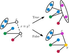
Figure 2: We test if $x$ and $y$ are in the same equivalence class. If they are, their vertices are contracted together. If they are not, an edge is added.

An equitable $k$-coloring of a graph is a proper coloring of a graph such that the size of each color class is either $\lfloor n/k\rfloor$ or $\lceil n/k\rceil$. A weighted equitable $k$-coloring of a vertex weighted graph is a proper coloring of a graph such that the sum of the weight in each color class is either $\lfloor n/k\rfloor$ or $\lceil n/k\rceil$. Examples of these can be seen in Figure 3.

Figure 3: On the left we have a graph with an equitable $3$-coloring and on the right we have a graph with a weighted equitable $3$-coloring.

An adversary for the problem of equivalence class sorting when every equivalence class has the same size $f$ (so $f$ divides $n$) must maintain that the graph has a weighted equitable $n/f$-coloring where the weights are the size of the vertex sets. The adversary we describe here will maintain such a coloring and additionally mark the elements and the color classes in a special way. It proceeds as follows.

First, initialize an arbitrary equitable coloring on the starting graph that consists of $n$ vertices and no edges. For each comparison of two elements done by the adversary algorithm, let us characterize how we react based on the following case analysis:

• If either of the elements is unmarked and this comparison would increase its degree to higher than $n/4f$, then mark it as having “high” element degree.

• If either element is still unmarked, they currently have the same color, and there is another unmarked vertex such that it is not adjacent to a vertex with the color involved in the comparison and no vertex with its color is adjacent to the unmarked vertex in the comparison (i.e. we can have it swap colors with one of the vertices in the comparison), then swap the color of that element and the unmarked element in the comparison.

• If either element is still unmarked, they currently have the same color, and there is no other unmarked vertex with a different unmarked color not adjacent to the color of the two elements being compared, then mark all elements with the color involved in the comparison as having “high” color degree and mark the color as having “high” degree.

• At this point, either both elements are marked and we answer based on their color, or one of the elements is unmarked and they have different colors, so we answer “not equal” to the adversary algorithm.

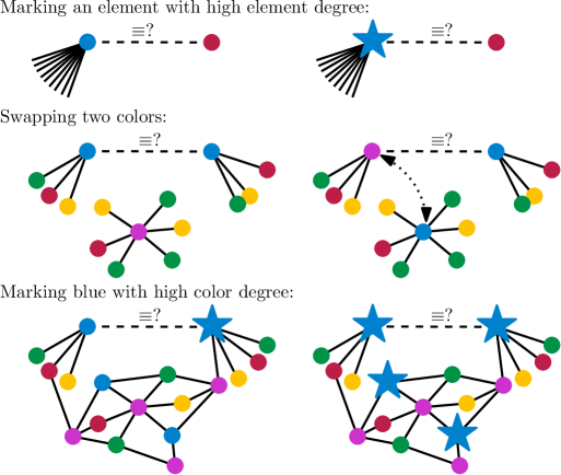
Figure 4: Three cases of how the adversary works to mark vertices and swap colors. The dashed line indicates the two elements being compared. Marked vertices are denoted with stars.

At all times, the vertices that contain unmarked elements all have weight one, because the adversary only answers equivalent for comparisons once both vertices are marked. When a color class is marked, all elements in that color class are marked as having “high” color degree. A few of the cases the adversary goes through are depicted in Figure 4.

Lemma 3.

If $n/8$ elements are marked during the execution of an algorithm, then $\Omega(n^{2}/f)$ comparisons were performed.

Proof.

There are three types of marked vertices: those with “high” element degree marks, those with “high” color degree marks, and those with both marks.

The color classes must have been marked as having “high” degree when a comparison was being performed between two elements of that color class and there were no unmarked color candidates to swap colors with. Because one of the elements in the comparison had degree less than $n/4f$, only a quarter of the elements have a color class it cannot be swapped with. So if there were at least $n-n/4$ unmarked elements in total, then the elements in the newly marked color class must have been in a comparison $n/2$ times.

The “high” element degree elements were involved in at least $n/4f$ comparisons each. So if $i$ color classes were marked and $j$ elements were only marked with “high” element degree, then the marked elements must have been a part of a test at least $ni/2+nj/4f\geq(i+j/f)n/4$ times. Once $if+j\geq n/8$, then at least $n^{2}/64f$ equivalence tests were performed. ∎

Theorem 5.

If every equivalence class has the same size $f$, then sorting requires at least $\Omega(n^{2}/f)$ equivalence comparisons.

Proof.

When an algorithm finishes sorting, each vertex will have weight $f$ and so the elements must all be marked. Thus, by Lemma 3, at least $\Omega(n^{2}/f)$ comparisons must have been performed. ∎

We also have the following lower bound as well.

Theorem 6.

Finding an element in the smallest equivalence class, whose size is $\ell$, requires at least $\Omega(n^{2}/\ell)$ equivalence comparisons.

Proof.

We use an adversary argument similar to the previous one, but we start with $\ell$ vertices colored a special smallest class color (scc) and seperate the remaining $n-\ell$ vertices into $\lfloor(n-\ell)/(\ell+1)\rfloor$ color classes of size $\frac{n}{\lfloor(n-\ell)/(\ell+1)\rfloor}$ or $\frac{n}{\lfloor(n-\ell)/(\ell+1)\rfloor}+1$.

There are two changes to the previous adversary responses. First, the degree requirement for having “high” degree is now $n/4\ell$. Second, if an scc element is about to be marked as having “high” degree, we attempt to swap its color with any valid unmarked vertex. Otherwise, we proceed exactly as before.

If an algorithm attempts to identify an element as belonging to the smallest equivalence class, no scc elements are marked, and there have been fewer than $n/8$ elements marked, then the identified element must be able to be swapped with a different color and the algorithm made a mistake. Therefore, to derive a lower bound for the total number of comparisons, it suffices to derive a lower bound for the number of equivalence tests until an scc element is marked.

The scc color class cannot be marked as having “high” color degree until at least one scc element has high element degree. However, as long as fewer than $n/8$ elements are marked, we will never mark an scc element with “high” degree. So at least $n/8$ elements need to be marked as having “high” element degree or “high” color degree and, by the same type of counting as in Lemma 3, $\Omega(n^{2}/\ell)$ equivalence tests are needed. ∎

4 Sorting Distributions

In this subsection, we study a version of the equivalence class sorting problem where we are given a distribution, $D$, on a countable set, $S$, and we wish to enumerate the set in order of most likely to least likely, $s_{0},s_{1},s_{2},\dots$. For example, consider the following distributions:

• Uniform: In this case, $D$ is a distribution on $k$ equivalence classes, with each equivalence class being equally likely for every element of $S$.

• Geometric: Here, $D$ is a distribution such that the $i$th most probable equivalence class has probability $p^{i}(1-p)$. Each element “flips” a biased coin where “heads” occurs with probability $p$ until it comes up “tails.” Then that element is in equivalence class $i$ if it flipped $i$ heads.

• Poisson: In this case, $D$ is model of the number of times an event occurs in an interval of time, with an expected number of events determined by a parameter $\lambda$. Equivalence class $i$ is defined to be all the samples that have the same number of events occurring, where the probability of $i$ events occurring is

  $$\frac{\lambda^{i}e^{-\lambda}}{i!}\ .$$

• Zeta: This distribution, $D$, is related to Zipf’s law, and models when the sizes of the equivalence classes follows a power law, based on a parameter, $s>1$, which is common in many real-world scenarios, such as the frequency of words in natural language documents. With respect to equivalence classes, the $i$th equivalence class has probability

  $$\frac{i^{-s}}{\zeta(s)},$$

  where $\zeta(s)$ is Riemann zeta function (which normalizes the probabilities to sum to 1).

So as to number equivalence classes from most likely to least likely, as $i=0,1,\ldots$, define $D_{\mathbb{N}}$ to be a distribution on the natural numbers such that

$$\Pr_{x\sim D_{\mathbb{N}}}\left[x=i\right]=\Pr_{y\sim D}\left[y=s_{i}\right].$$

Furthermore, so as to “cut off” this distribution at $n$, define $D_{\mathbb{N}}(n)$ to be a distribution on the natural numbers less than or equal to $n$ such that, for $0\leq i<n$,

$$\Pr_{x\sim D_{\mathbb{N}}(n)}\left[x=i\right]=\Pr_{y\sim D_{\mathbb{N}}}\left[y=i\right]$$

and

$$\Pr_{x\sim D_{\mathbb{N}}(n)}\left[x=n\right]=\Pr_{y\sim D_{\mathbb{N}}}\left[y\geq n\right].$$

That is, we are “piling up” the tail of the $D_{\mathbb{N}}$ distribution on $n$.

The following theorem shows that we can use $D_{\mathbb{N}}(n)$ to bound the number of comparisons in an ECS algorithm when the equivalence classes are drawn from $D$. In particular, we focus here on an algorithm by Jayapaul et al. [12] for equivalence class sorting, which involves a round-robin testing regiment, such that each element, $x$, initiates a comparison with the next element, $y$, with an unknown relationship to $x$, until all equivalence classes are known.

Theorem 7.

Given a distribution, $D$, on a set of equivalence classes, then $n$ elements who have corresponding equivalence class independently drawn from $D$ can be equivalence class sorted using a total number of comparisons stochastically dominated by twice the sum of $n$ draws from the distribution $D_{\mathbb{N}}(n)$.

Proof.

Let $V_{i}$ denote the random variable that is equal to the natural number corresponding to the equivalence class of element $i$ in $D_{\mathbb{N}}(n)$. We denote the number of elements in equivalence class $i$ as $Y_{i}$. Let us denote the number of equivalence tests performed by the algorithm by Jayapaul et al. [12] using the random variable, $R$.

By a lemma from [12], for any pair of equivalence classes, $i$ and $j$, the round-robin ECS algorithm performs at most $2\min(Y_{i},Y_{j})$ equivalence tests in total. Thus, the total number of equivalence tests in our distribution-based analysis is upper bounded by

$$R \leq \sum_{i=0}^{\infty}\sum_{j=0}^{i-1}2\min(Y_{i},Y_{j})$$

$$= 2\sum_{i=0}^{n}\sum_{j=0}^{i-1}\min(Y_{i},Y_{j})+2\sum_{i=n+1}^{\infty}\sum_{j=0}^{i-1}\min(Y_{i},Y_{j})$$

$$\leq 2\sum_{i=0}^{n}\sum_{j=0}^{i-1}Y_{i}+2\sum_{i=n+1}^{\infty}nY_{i}$$

$$\leq 2\left(\sum_{i=0}^{n}iY_{i}+\sum_{i=n+1}^{\infty}nY_{i}\right)=2\sum_{i=1}^{n}V_{i}$$

The second line in the above simplification is a simple separation of the double summation and the third line follows because $\sum_{j=0}^{i-1}\min(Y_{i},Y_{j})$ is zero if $Y_{i}$ is zero and at most $n$, otherwise. So the total number of comparisons in the algorithm is bounded by twice the sum of $n$ draws from $D_{\mathbb{N}}(n)$. ∎

Given this theorem, we can apply it to a number of distributions to show that the total number of comparisons performed is linear with high probability.

Theorem 8.

If $D$ is a discrete uniform, a geometric, or a Poisson distribution on a set equivalence classes, then it is possible to equivalence class sort using linear total number of comparisons with exponentially high probability.

Proof.

The sum of $n$ draws from $D_{\mathbb{N}}(n)$ is stochastically dominated by the sum of $n$ draws from $D_{\mathbb{N}}$. Let us consider each distribution in turn.

• Uniform: The sum of $n$ draws from a discrete uniform distribution is bounded by $n$ times the maximum value.

• Geometric: Let $p$ be the parameter of a geometric distribution and let $X=\sum_{i=0}^{n-1}X_{i}$ where the $X_{i}$ are drawn from $\mathop{Geom}(p)$, which is, of course, related to the Binomial distribution, $\mathop{Bin}(n,p)$, where one flips $n$ coins with probability $p$ and records the number of “heads.” Then, by a Chernoff bound for the geometric distribution (e.g., see [14]),

  $$\Pr[X-(1/p)n>k] = \Pr[\mathop{Bin}(k+(1/p)n,p)<n]$$

  $$\leq e^{-2\frac{(pk+n-n)^{2}}{k+(1/p)n}}$$

  $$\Pr[X>(2/p)n] \leq e^{-np}$$

• Poisson: Let $\lambda$ be the parameter of a Poisson distribution and let $Y=\sum_{i=0}^{n-1}Y_{i}$ where the $Y_{i}$ are drawn from $\mathop{Poisson}(\lambda)$. Then, by a Chernoff bound for the Poisson distribution (e.g., see [14]),

  $$\Pr[Y>(\lambda(e-1)+1)n] = \Pr[e^{Y}>e^{(\lambda(e-1)+1)n}]$$

  $$\leq \frac{(E[e^{Y_{i}}])^{n}}{e^{(\lambda(e-1)+1)n}}$$

  $$= \frac{e^{\lambda(e-1)n}}{e^{(\lambda(e-1)+1)n}}=e^{-n}$$

So, in each case with exponentially high probability, the sum of $n$ draws from the distribution is $O(n)$ and the round-robin algorithm does $O(n)$ total equivalence tests. ∎

We next address the zeta distribution.

Theorem 9.

Given a zeta distribution with parameter $s>2$, $n$ elements who have corresponding equivalence class independently drawn from the zeta distribution can be equivalence class sorted in $O(n)$ work in expectation.

Proof.

When $s>2$, the mean of the zeta distribution is

$$\frac{\zeta(s-1)}{\zeta(s)},$$

which is a constant. So the sum of $n$ draws from the distribution is expected to be linear. Therefore, the expected total number of comparisons in the round-robin algorithm is linear. ∎

Unfortunately, for zeta distributions it is not immediately clear if it is possible to improve the above theorem so that total number of comparisons is shown to be linear when $2\geq s>1$ or obtain high probability bounds on these bounds. This uncertainty motivates us to look experimentally at how different values of $s$ cause the runtime to behave. Likewise, our high-probability bounds on the total number of comparisons in the round-robin algorithm for the other distibutions invites experimental analysis as well.

5 Experiments

In this section, we report on experimental validatations of the theorems from the previous section and investigations of the behavior of running the round-robin algorithm on the zeta distribution. For the uniform, geometric, and Poisson distributions, we ran ten tests on sizes of $10,000$ to $200,000$ elements incrementing in steps of $10,000$. For the zeta distribution, because setting $s<2$ seems to lead to a super linear number of comparisons, we reduced the test sizes by a factor of $10$ and ran ten tests each on sizes from $1,000$ to $20,000$ in increments of $1,000$. For each distribution we used the following parameter settings for various experiments:

Uniform:	$k=10,25,100$
Geometric:	$p=\frac{1}{2},\frac{1}{10},\frac{1}{50}$
Poisson:	$\lambda=1,5,25$
Zeta:	$s=1.1,1.5,2,2.5$

The results of these tests are plotted in Figure 5. Best fit lines were fitted whenever we have theorems stating that there will be a linear number of comparisons with high probability or in expectation (i.e., everything except for zeta with $s<2$). We include extra plots of the zeta distribution tests with the $s=1.1$ data and the $s=1.1,1.5$ data removed to better see the other data sets.

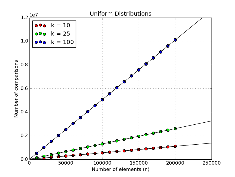
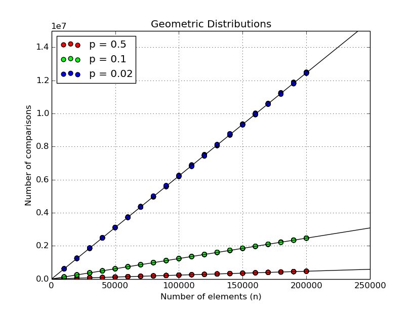
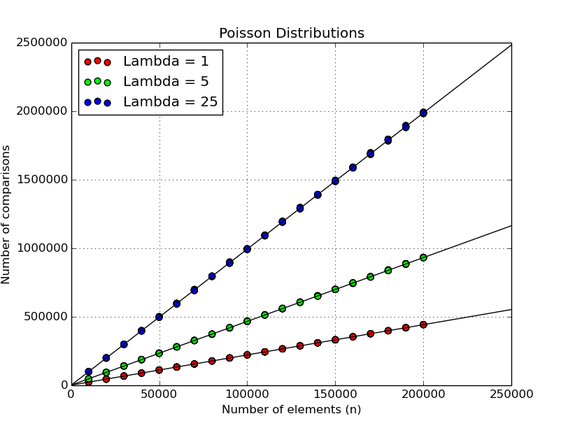
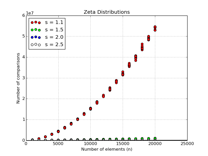
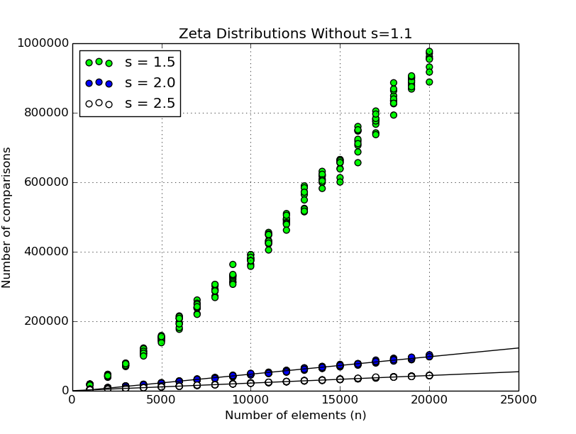
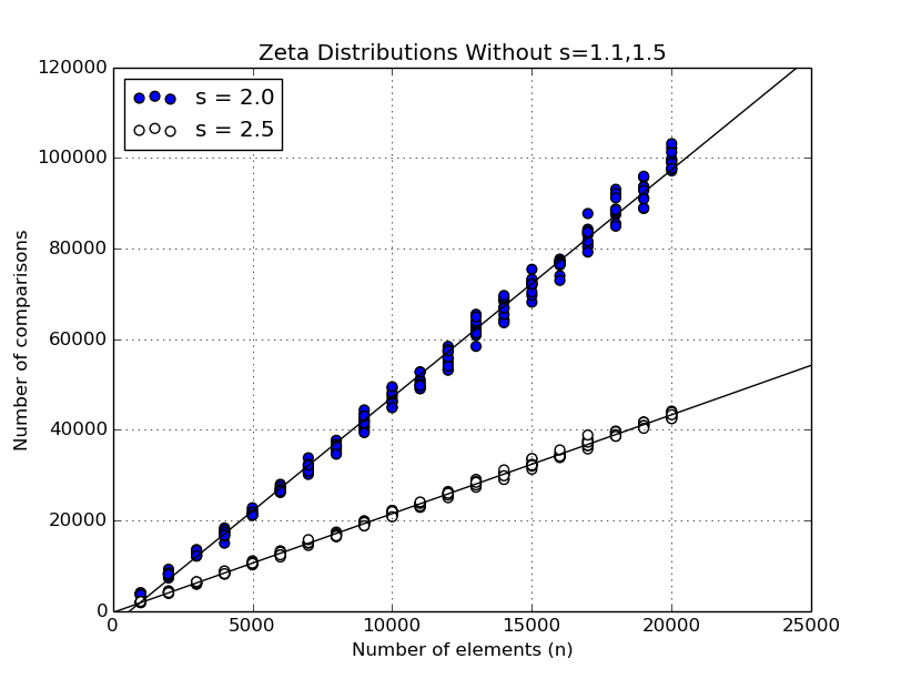
Figure 5: The results of the experiments are plotted and best fit lines are placed when we have a linear number of comparisons with high probability or in expectation.

We can see from the data that the number of comparisons for the uniform, geometric, and Poisson distributions are so tightly concentrated around the best fit line that only one data point is visible. Contrariwise, the data points for the zeta distributions do not cluster nearly as nicely. Even when we have linear expected comparisons with $s=2$, the data points vary by as much as $10\%$.

6 Conclusion

In this paper we have studied the equivalence class sorting problem, from a parallel perspective, giving several new algorithms, as well as new lower bounds and distribution-based analysis. We leave as open problems the following interesting questions:

• Is it possible to find all equivalance classes in the ER version of the ECS problem in $O(k)$ parallel rounds, for $k\geq 3$, where $k$ is the number of equivalence classes? Note that the answer is “yes” for $k=2$, as it follows from previous results for the parallel fault diagnosis problem [5, 6, 4].

• Is it possible to bound the number of comparisons away from $O(n^{2})$ for the zeta distribution when $s<2$ even just in expectation?

• Is it possible to prove a high-probability concentration bound for the zeta distribution, similar to the concentration bounds we proved for other distributions?

Acknowledgments

This research was supported in part by the National Science Foundation under grant 1228639 and a gift from the 3M Corporation. We would like to thank David Eppstein and Ian Munro for several helpful discussions concerning the topics of this paper.

References

- [1] L. Alonso and E. M. Reingold. Analysis of Boyer and Moore’s MJRTY algorithm. Information Processing Letters, 113(13):495–497, 2013.
- [2] L. Alonso, E. M. Reingold, and R. Schott. Determining the majority. Information Processing Letters, 47(5):253 – 255, 1993.
- [3] L. Babai, P. Erdös, and S. M. Selkow. Random graph isomorphism. SIAM Journal on Computing, 9(3):628–635, 1980.
- [4] R. Beigel, W. Hurwood, and N. Kahale. Fault diagnosis in a flash. In 36th IEEE Symp. on Foundations of Computer Science (FOCS), pages 571–580, 1995.
- [5] R. Beigel, S. R. Kosaraju, and G. F. Sullivan. Locating faults in a constant number of parallel testing rounds. In 1st ACM Symp. on Parallel Algorithms and Architectures (SPAA), pages 189–198, 1989.
- [6] R. Beigel, G. Margulis, and D. A. Spielman. Fault diagnosis in a small constant number of parallel testing rounds. In 5th ACM Symp. on Parallel Algorithms and Architectures (SPAA), pages 21–29, 1993.
- [7] C. Castelluccia, S. Jarecki, and G. Tsudik. Secret handshakes from CA-oblivious encryption. In P. J. Lee, editor, Advances in Cryptology - ASIACRYPT, pages 293–307. Springer, 2004.
- [8] D. J. Cook and L. B. Holder. Mining Graph Data. John Wiley & Sons, 2006.
- [9] D. Dobkin and J. I. Munro. Determining the mode. Theoretical Computer Science, 12(3):255–263, 1980.
- [10] M. T. Goodrich. Pipelined algorithms to detect cheating in long-term grid computations. Theoretical Computer Science, 408(2–3):199–207, 2008.
- [11] S. Jarecki and X. Liu. Unlinkable secret handshakes and key-private group key management schemes. In J. Katz and M. Yung, editors, 5th Int. Conf. on Applied Cryptography and Network Security (ACNS), pages 270–287. Springer, 2007.
- [12] V. Jayapaul, J. I. Munro, V. Raman, and S. R. Satti. Sorting and selection with equality comparisons. In F. Dehne, J.-R. Sack, and U. Stege, editors, 14th Int. Symp. on Algorithms and Data Structures (WADS), pages 434–445. Springer, 2015.
- [13] L. Kozma. Useful inequalities cheat sheet, 2016. http://www.lkozma.net/inequalities_cheat_sheet/.
- [14] M. Mitzenmacher and E. Upfal. Probability and Computing: Randomized Algorithms and Probabilistic Analysis. Cambridge University Press, 2005.
- [15] H. Orman. The Morris worm: A fifteen-year perspective. IEEE Security & Privacy, 1(5):35–43, 2003.
- [16] S. Parthasarathy, S. Tatikonda, and D. Ucar. A survey of graph mining techniques for biological datasets. In C. C. Aggarwal and H. Wang, editors, Managing and Mining Graph Data, pages 547–580. Springer, 2010.
- [17] A. Pelc and E. Upfal. Reliable fault diagnosis with few tests. Combinatorics, Probability and Computing, 7:323–333, 1998.
- [18] F. P. Preparata, G. Metze, and R. T. Chien. On the connection assignment problem of diagnosable systems. IEEE Trans. on Electronic Computers, EC-16(6):848–854, 1967.
- [19] M. E. Saks and M. Werman. On computing majority by comparisons. Combinatorica, 11(4):383–387, 1991.
- [20] A. Sorniotti and R. Molva. A provably secure secret handshake with dynamic controlled matching. Computers & Security, 29(5):619–627, 2010.
- [21] L. G. Valiant. Parallelism in comparison problems. SIAM Journal on Computing, 4(3):348–355, 1975.
- [22] S. Xu and M. Yung. K-anonymous secret handshakes with reusable credentials. In 11th ACM Conf. on Computer and Communications Security (CCS), pages 158–167, 2004.