Effect of magnetic field on a magnetic topological insulator film with structural inversion asymmetry

Abstract

The effect of magnetic field on an ultrathin magnetic topological insulator film with structural inversion asymmetry is investigated. We introduce the phase diagram, calculate the Landau-level spectrum analytically and simulate the transport behavior in Landauer-Büttiker formalism. The quantum anomalous Hall phase will survive increasing magnetic field. Due to the two spin polarized zero modes of Landau levels a nontrivial phase similar with quantum spin Hall effect can be induced by magnetic field which is protected by structural inversion symmetry. Some exotic longitudinal and Hall resistance plateaus with fractional values are also found in a six terminal Hall bar, arising from the coupling between edge states due to inverted energy band and Landau levels.

I Introduction

The quantum Hall effect (QHE),IQHE as a quantized version of Hall effect,Halleffect occurs when dissipationless chiral edge states form at sample edges due to the Landau level (LL) quantization in the perpendicular magnetic field. QHE is also suggested to exist without LLs and magnetic field.QAH(Haldane) ; QAH(proposal) ; Yu(science) In this type of QHE, the chiral edge states are due to the inverted energy band structure. It is considered the quantized version of the anomalous Hall effectAHE_E and named as quantum anomalous Hall (QAH) effect. If time reversal symmetry (TRS) is preserved, counterpropagate dissipationless edge states can form due to inverted energy band structure,QSH_T which is named quantum spin Hall (QSH) effect as a quantized version of spin Hall effect.SpinHall In QSH effect, two counterpropagate spin polarized edge states will vanish the Hall resistance while the longitudinal resistance is quantized to be $h/(2e^{2})$.QSH_E ; jiang1 QSH effect is soon discoveredQSH_E after the prediction.QSH_T However the QAH effect is observed very recently by Chang $et$ $al$Xue_QAH though predicted much earlier.QAH(Haldane)

In Ref.(Xue_QAH ), QAH effect is observed in a magnetically doped topological insulator (TI) film. The TI is a new phase of matter which behaves as an insulator in the bulk but has dissipationless edge states (two dimensional) or surface states (three dimensional).review(Ti) The low energy excitation is the massless Dirac fermion for isolated surface states. But if the TI film is thin enough, inter-surface tunnelling will occur resulting in an energy gap to make the excitation massive.NJP(Shan) ; PRB(Lu) By magnetically doping the TI film, ferromagnetic order will form resulting in an exchange field at low temperature. If the exchange field overcomes the energy gap and is perpendicular to the film, QAH effect will occur.Yu(science) With gates on both surfaces of the film, the potential of each surface as well the Fermi energy of the sample can be tuned conveniently. The potential difference between two surfaces acts as a structure inversion asymmetry (SIA) term. In Ref.(Xue_QAH ) measurement under magnetic field is also performed, but only the QAH resistivity plateau is observed even in a strong magnetic field. The QHE keeps missing because of the low mobility of the sample. Therefore it’s still unknown how the QAH effect and QHE will interplay and what’s the effect of SIA potential in presence of magnetic field.

Existing literature mainly focus on the LL spectrum in two dimensional (2D) infinite TI film.effective_H_Liu ; QSH_E ; LLTIfilm ; PRB(L.Sheng) ; JAPLL In a perpendicular magnetic field, both the massless and massive Dirac fermions will quantize into LLs.book_QED1965 The isolated surface state accounts for the massless caseeffective_H_Liu and the $\mathbb{k}$-independent inter-surface tunneling acts as the mass term which can be tuned by the thickness.LLTIfilm Indeed there has already been several experimental progress. The quantized LLs for massless Dirac fermions have been measured in $Bi_{2}Se_{3}$,DiracLL_TI_E $Sb_{2}Te_{3}$,PRL(Y.P.Jiang) $Bi_{2}Te_{3}$,DLL(Okada) and $HgTe$.DLL(HgTe) However the effect of $\mathbb{k}$-dependent inter-surface tunneling, SIA potential and exchange field is still not studied theoretically. The $\mathbb{k}$-dependent tunneling will make two zero modes of LLs linearly depend on the magnetic field and cross to form a QSH-like phase. SIA potential term is necessary to describe the potential distribution in the perpendicular direction even for a film grown on a substrate with a single back gate.lu2013QAH

Few work focuses on the transport simulation to understand the interplay between QAH effect and QHE. Though LL spectrum is helpful, transport simulation is still necessary to give a complete explanation. The reason is that edge state occurs at the boundary, then only in a finite size sample the coupling between the edge state due to inverted band structure and edge state due to LLs are uncovered directly. Indeed, the coupling gives rise to exotic behavior missing in LL spectrum.

In this paper we study the property of a magnetic TI film with SIA in a perpendicular magnetic field. Both the LL spectrum and transport simulation are investigated. The two zero modes are spin polarized with opposite Chern number to form a QSH-like phase protected by structural inversion symmetry at small magnetic field. Magnetic field can’t break the QAH phase with Chern number $C=1$. When it comes to the case of nanoribbon with open boundary condition, the edge state due to the inverted band structure will couple with the edge state due to LLs at the same edge to form an exotic energy band. Correspondingly exotic resistance plateaus with nonzero longitudinal component can be observed in a six terminal Hall bar. Besides we find that it’s helpful to classify the LLs according to the energy band they correspond to. The coupling between edge state due to inverted energy band and edge states due to LLs corresponding to trivial energy band is weaker than that to nontrivial band.

The rest of the paper is organized as follows. In Sec. II, we introduce the Hamiltonian and the phase diagram in absence of magnetic field. In Sec. III, we derive the LL spectrum in the infinite system analytically. In Sec. IV, we study the transport properties of the six-terminal system in Landauer-Büttiker formalism. A summary is given in the last section.

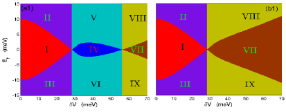
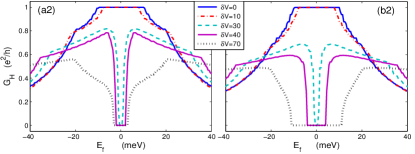
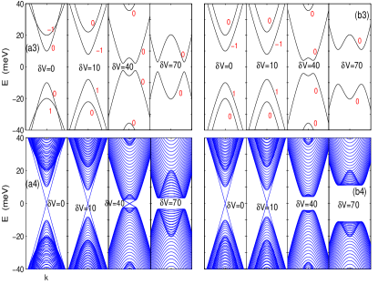
Figure 1: (Color online) (a1,b1) phase diagrams in the plane of SIA potential $\delta V$ and Fermi energy $E_{f}$. Regions I-VI are in inverted regime. Region I (IV) is the QAH (QPH) phase with Fermi level in the bulk gap, and II,V (III,VI) are the n(p)-doped inverted system. Region VII is the normal insulator phase with Fermi level in the bulk gap. Regions VIII and IX are in normal metal phase. (a2,b2) Hall conductance as a function of Fermi energy for several $\delta V$. (a3,b3) the energy dispersion of the 2D system in a certain direction. (a4,b4) the energy dispersion of a nanoribbon with the ribbon width $480nm$. (a1-4) for $m_{0}/B<0$ and (b1-4) for $m_{0}/B>0$ with the exchange field $M=-15meV$. Energy in unit of $meV$ in this paper if not indicated.

II Hamiltonian and Phase diagram

The effective Hamiltonian near the $\Gamma$ point for bulk $Bi_{2}Se_{3}$ is given byHJZhang

$$H_{bulk}\!\!=\!\!\epsilon_{0}({\mathbb{k}})I_{4\times 4}\!\!+\!\!\left(\begin{array}[]{cccc}M({\mathbb{k}})&-iA_{1}\partial_{z}&0&A_{2}k_{-}\\ -iA_{1}\partial_{z}&-M({\mathbb{k}})&A_{2}k_{-}&0\\ 0&A_{2}k_{+}&M({\mathbb{k}})&iA_{1}\partial_{z}\\ A_{2}k_{+}&0&iA_{1}\partial_{z}&-M({\mathbb{k}})\end{array}\right),$$ (5)

in the basis formed by the hybridized states of $Se$ and $Bi$ $p_{z}$ orbitals, denoted as $(|p1_{z}^{+},\!\uparrow\rangle,|p2_{z}^{-},\!\uparrow\rangle,|p1_{z}^{+},\!\downarrow\rangle,|p2_{z}^{-},\!\downarrow\rangle)^{T}$. where $k_{\pm}=k_{x}\pm ik_{y}$, $\epsilon_{0}({\mathbb{k}})=C-D_{1}\partial_{z}^{2}+D_{2}k^{2}$, $M({\mathbb{k}})=M+B_{1}\partial_{z}^{2}-B_{2}k^{2}$, and $k^{2}=k_{x}^{2}+k_{y}^{2}$, with $A_{1}$, $A_{2}$, $B_{1}$, $B_{2}$, $C$, $D_{1}$, $D_{2}$ and $M$ being the model parameters.

For a thin film with surfaces perpendicular to the $z$-direction, surface states will emerge with effective HamiltonianYu(science) ; note1

$$H_{sf}=\tilde{A}_{2}(k_{y}\sigma_{x}\!-\!k_{x}\sigma_{y})\tau_{z}+m_{k}\tau_{x},$$ (7)

in basis $(|t\!\uparrow\rangle,\,|t\!\downarrow\rangle,|b\!\uparrow\rangle,\,|b\!\downarrow\rangle)^{T}$, where $t\,\,(b)$ represents the top (bottom) surface states and $\uparrow(\downarrow)$ represent the up(down)-spin states. $|\!\!\uparrow\!\!(\downarrow)\!\rangle$ is the superposition of the up(down)-spin hybridized states of $Se$ and $Bi$ $p_{z}$ orbitals. $\sigma_{x,y,z}$ and $\tau_{x,y,z}$ are Pauli matrices acting on spin space and mixing the top and bottom surface states respectively. The first term in Hamiltonian describes the free surface states with $\tilde{A}_{2}=\hbar v_{F}$ describing the Fermi velocity of surface state. The second term is the coupling between the top and bottom surface states with $m_{k}=m_{0}+Bk^{2}$. Inter-surface tunneling will open a gap with width $2m_{0}$, then the ultrathin three dimensional TI film is in QSH phase with two inverted band structure for $m_{0}/B<0$ and topological trivial phase for $m_{0}/B>0$ depending on film thickness.Yu(science) ; QSH_NI_Osci(Liu) ; NJP(Shan) ; PRB(L.Sheng2012)

Then the Hamiltonian of the thin magnetic TI film with electric potential on both surfaces can be written as,

$$H\!=H_{sf}+\!M\sigma_{z}\!+\!\frac{\delta V}{2}\tau_{z}$$ (8)

The second term is due to the exchange field along $z$ direction to describe the ferromagnetic order induced by magnetic dopants. It acts just like the Zeeman energy. A moderate enough exchange field ($|M|>|m_{0}|$) will alter the energy band resulting in only one inverted band to give rise to the QAH phase both for $m_{0}/B<0$ and $m_{0}/B>0$ . The last term is the SIA potential, i.e. it describes the effect of the gate voltages on top and bottom surfaces with magnitudes $\pm\delta V/2$ respectively.

There is only a difference of unitary transformation between $H(-\delta V,m_{k},v_{F},M)$, $H(\delta V,-m_{k},v_{F},M)$, $H(\delta V,m_{k},-v_{F},M)$, $-H(\delta V,m_{k},v_{F},-M)$ and $H(\delta V,m_{k},v_{F},M)$. Therefore we only consider the positive SIA potential $\delta V$, the positive $m_{0}$ and the negative $M$. Accordingly parameters in Hamiltonian are chosen as $v_{F}=4.53\times 10^{5}ms^{-1}$, $m_{0}=5meV$ and $B=\pm 800meV\cdot nm^{2}$ in this paper.nphys(Y.Zhang) Both cases $m_{0}/B<0$ and $m_{0}/B>0$ are studied respectively. For the case $M=0$ the system lies in QSH phase which has been studied in detail and well understood.review(Ti) ; QSH_E ; PRB_HgTe(J.C.Chen) ; jiang2 Therefore we mainly focus on the case $|M|>m_{0}$ and set $M=-15meV$ so that the QAH phase will emerge for both $m_{0}/B<0$ and $m_{0}/B>0$ in absence of SIA potential ($\delta V=0$).

The continuous energy band of the Hamiltonian (8) is derived as,

$$\epsilon^{2} = \hbar^{2}v_{F}^{2}k^{2}+m_{k}^{2}+M^{2}+\delta V^{2}/4$$ (9)

$$\pm 2\sqrt{m_{k}^{2}M^{2}+M^{2}\delta V^{2}/4+\hbar^{2}v_{F}^{2}k^{2}\delta V^{2}/4}.$$

An energy gap can be opened by the inter-surface tunneling $m_{k}$, exchange field $M$ or SIA potential $\delta V$. There are two branches split by exchange field and SIA potential in both electron-like and hole-like energy bands. Fig.1 (a3,b3) show energy dispersion curves. The two branches will cross for $m_{0}/B<0$ and $\delta V=0$. However, even a tiny $\delta V$ can break the crossing. In the following we will show that this crossing leads to interesting phenomena.

Tuning the potential difference $\delta V$ adiabatically, the energy gap will close and reopen according to Eq.(9). For $m_{0}/B<0$ the gap closing occurs twice for $|\delta V|/2=\sqrt{M^{2}-m_{0}^{2}}$ at $\Gamma$ point and $|\delta V|/2=\sqrt{M^{2}+\hbar^{2}v_{F}^{2}|m_{0}/B|}$ at $|\mathbb{k}|\!=\!\sqrt{-m_{0}/B}$ in $\mathbb{k}$-space as shown in Fig.1(a1). For the $m_{0}/B<0$ case, the gap only closes and reopens once for $|\delta V|/2=\sqrt{M^{2}-m_{0}^{2}}$ at $\Gamma$ point. Fig.1(a/b1) show the phase diagram in the plane of the SIA potential $\delta V$ and Fermi energy $E_{f}$, in which nine regions emerge for the $m_{0}/B<0$ case and six regions for the $m_{0}/B>0$ case. To determine the topological property of each region we calculate the Chern number which equals the zero-temperature Hall conductance by $G_{H}\!=\!C\frac{e^{2}}{h}$ and can be calculated via the Kubo formulaKuboChern ; note2

$$G_{H}\!\!=\!\!\frac{2e^{2}}{\hbar}\int_{BZ}\frac{dk_{x}dk_{y}}{(2\pi)^{2}}\!\!\sum_{\epsilon_{l}<E_{f}<\epsilon_{n}}\!\!\!Im\frac{\langle l|\frac{\partial H}{\partial k_{x}}|n\rangle\langle n|\frac{\partial H}{\partial k_{y}}|l\rangle}{(\epsilon_{l}-\epsilon_{n})^{2}},$$ (10)

where BZ represents first Brillouim zone, and $\epsilon_{l/n}$ and $|l/n\rangle$ are the corresponding eigenenergy and eigenstate respectively. Results shown in Fig.1(a2,b2) indicate that regions I-III in Fig.1(a1,b1) are in inverted regime. To determine the property of regions IV-IX, we calculate the energy dispersion of a nanoribbon with open boundary condition along $y$ direction to check directly whether an edge state exists or not. Results in Fig.1(a4,b4) suggest that regions IV-VI and VII-IX are in inverted regime and normal insulator regime respectively. And region IV is a quantum pseudo-spin (QPH) phaseNJP(Shan) ; PRB(L.Sheng2012) with two counterpropagating edge states at the same edge of the sample. In short it goes through QAH phase, QPH phase and normal insulator phase as $\delta V$ increases from zero for $m_{0}/B<0$. In contrast, in the case $m_{0}/B>0$, it directly goes from QAH phase to the normal insulator phase, and the QPH phase doesn’t appear.

Integers in Fig.1(a2,b2) show the Chern number of the corresponding band. From Fig.1(a4,b4) and the Chern number, we indicate that the inner (outer) two bands are trivial (nontrivial) for $m_{0}/B<0$ but nontrivial (trivial) for $m_{0}/B>0$ in absence of SIA potential ($\delta V=0$). But even for a small nonzero SIA potential $\delta V$, the two inner bands are nontrivial and the outer ones are trivial in the inverted regime. While $\delta V$ is large enough ($\delta V/2>\sqrt{M^{2}-m_{0}^{2}}$ for $m_{0}/B>0$ or $\delta V/2>\sqrt{M^{2}+\hbar^{2}v^{2}_{F}|m_{0}/B|}$ for $m_{0}/B<0$), the system is in the normal regime, and then all four bands are trivial.

III magnetic field and Landau levels

In this section the LL spectrum of the 2D infinite system is studied. It is useful for understanding magnetic properties, such as the Hall effect, magneto-optics and Shubnikov-de Haas oscillation.

Magnetic fields will induce two types of contributions, the orbital effect and the Zeeman effect. The Zeeman term takes the same form as the exchange field but with a lesser order of magnitude. Therefore the Zeeman term can be neglected in the effective Hamiltonian. The orbital effect can be included by Peierls substitution $\mathbb{k}\to\mathbb{\pi}=\mathbb{k}+\frac{e}{\hbar}\mathbb{A}$ in which $\mathbb{A}=(B_{z}y,0,0)$ for magnetic field $(0,0,-B_{z})$ and $e$ is the magnitude of electron charge. To calculate the LL spectrum we define the annihilation and creation operator for the harmonic oscillator function $\phi_{N}$ as $\hat{a}=l_{c}\pi_{+}/\sqrt{2},\,\hat{a}^{\dagger}=l_{c}\pi_{-}/\sqrt{2}$ satisfying $[\hat{a},\hat{a}^{\dagger}]=1$, $\hat{a}\,\phi_{N}=\sqrt{N}\phi_{N-1}$, $\hat{a}^{\dagger}\,\phi_{N}=\sqrt{N+1}\phi_{N+1}$ with $l_{c}=\sqrt{\frac{\hbar}{eB_{z}}}$, $\pi_{\pm}=\pi_{x}\pm i\pi_{y}$ and $N=1,2,3,...$ .PRL(2004)(S.Q.Shen)(SR) Then the Hamiltonian can be written as

$$\tilde{H}\!=\!\!\left(\!\begin{array}[]{cccc}M+\delta V/2&i\omega_{1}a^{\dagger}&m_{N}-\alpha/2&0\\ -i\omega_{1}a&-M+\delta V/2&0&m_{N}-\alpha/2\\ m_{N}-\alpha/2&0&M-\delta V/2&-i\omega_{1}a^{\dagger}\\ 0&m_{N}-\alpha/2&i\omega_{1}a&-M-\delta V/2\end{array}\!\right)\\$$

in which $m_{N}=m_{0}-\alpha\hat{a}^{\dagger}\hat{a}$, $\omega_{1}=v_{F}\sqrt{2eB_{z}\hbar}$ and $\alpha=-\frac{2eB_{z}B}{\hbar}$. With the wave function ansatz $\psi_{N}=(f_{1}^{N}\phi_{N},f_{2}^{N}\phi_{N-1},f_{3}^{N}\phi_{N},f_{4}^{N}\phi_{N-1})^{T}$, the Hamiltonian can be written as

$$\tilde{H}^{\prime}\!\!=\!\!\left(\begin{array}[]{cccc}M+\delta V/2&i\omega_{N}&\tilde{m}_{N}-\alpha/2&0\\ -i\omega_{N}&-M+\delta V/2&0&\tilde{m}_{N}+\alpha/2\\ \tilde{m}_{N}-\alpha/2&0&M-\delta V/2&-i\omega_{N}\\ 0&\tilde{m}_{N}+\alpha/2&i\omega_{N}&-M-\delta V/2\end{array}\!\!\right)\!\!\!\!\!\!\!$$ (15)

in which $\tilde{m}_{N}=m_{0}-\alpha N$ and $\omega_{N}=v_{F}\sqrt{2e\hbar B_{z}N}$. Then LLs can be solved from the secular equation straightforwardly.

The zero mode of LLs can be derived as $E_{0\pm}=M\pm\sqrt{(m_{0}-\alpha/2)^{2}+(\delta V/2)^{2}}$ with wave function $\psi_{0}=(f_{1}^{0}\phi_{0},0,f_{3}^{0}\phi_{0},0)^{T}$. In absence of SIA potential, the two branches are defined as $E_{0\pm}=M\pm(m_{0}+\frac{eBB_{z}}{\hbar})$ which depends linearly on magnetic field. However the general analytical expression for nonzero modes is tediously long. Here we only analytically give the solutions in which case the electron-like and hole-like nonzero modes are symmetrical:

case I: $B=0$, with only lowest-order inter-surface tunnelling,

$$E_{N}^{2}= \omega_{N}^{2}+(\frac{\delta V}{2})^{2}+M^{2}+m_{0}^{2}$$

$$\pm 2\sqrt{\omega_{N}^{2}(\frac{\delta V}{2})^{2}+(\frac{\delta V}{2})^{2}M^{2}+M^{2}m_{0}^{2}},$$ (17)

case II: $M=0$, undoped TI film,

$$E_{N}^{2}= \omega_{N}^{2}+(\frac{\delta V}{2})^{2}+(\frac{\alpha}{2})^{2}+\tilde{m}_{N}^{2}$$

$$\pm 2\sqrt{\omega_{N}^{2}(\frac{\delta V}{2})^{2}+(\frac{\delta V}{2})^{2}(\frac{\alpha}{2})^{2}+(\frac{\alpha}{2})^{2}\tilde{m}_{N}^{2}}.$$ (18)

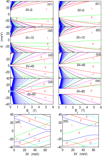
Figure 2: (Color online) Landau level spectrum. (a/b1-4) LLs as a function of magnetic field for several $\delta V$. (a/b5) LLs as a function of $\delta V$ for $B_{z}=3T$. Light green lines are the zero modes $E_{0\pm}$. $E_{0-}$ is the one lies below at small magnetic field. Red integers indicate the Chern number. (a1-5) for $m_{0}/B<0$, (b1-5) for $m_{0}/B>0$. The exchange field $M=-15meV$.

By eliminating the extra terms, i.e. inter-surface tunneling $m_{k}$, exchange field $M$ and SIA potential $\delta V$, the LL spectrum of Dirac electrons with linear energy dispersion is reduced into $E_{N}=sign(N)v_{F}\sqrt{2eB_{z}\hbar|N|}$ with $N=0,\pm 1,\pm 2...$ which is the well known result.book_QED1965 ; DiracLL_graphene_E However, the existence of these terms makes the dependence on $N$ and $B_{z}$ complex. Exchange field will break the symmetry of electron-like and hole-like LLs. LLs will emerge and split to realize fascinating phases by varying the magnetic field and SIA potential as is shown in Fig.2.

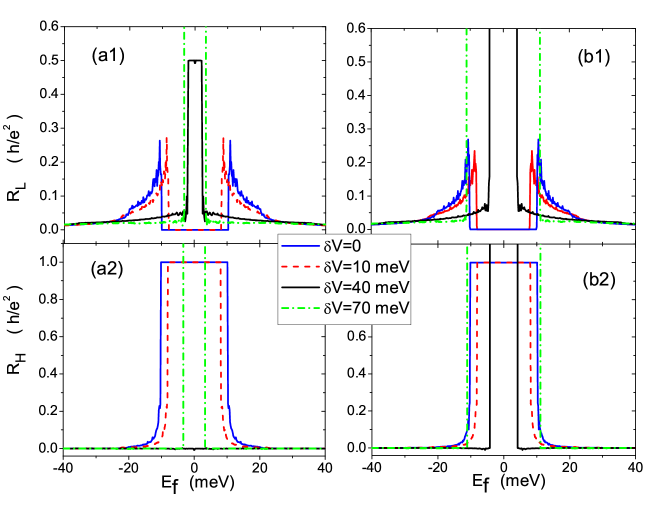
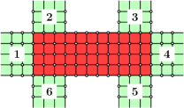
Figure 3: (Color online) Hall resistance $R_{H}$ and longitudinal resistance $R_{L}$ as a function of Fermi energy $E_{f}$ for several SIA terms in absence of magnetic field. (a1-2) for $m_{0}/B<0$, (b1-2) for $m_{0}/B>0$. Inset is the schematic of the Hall bar. The width of both the central region and six contacts is $480nm$.

If magnetic field is close to zero, $B_{z}\approx 0$, the nonzero LLs will converge at $E_{N}\approx\pm(M\pm\sqrt{m_{0}^{2}+\delta V^{2}/4})$ while zero modes at $E_{0\pm}\approx M\pm\sqrt{m_{0}^{2}+\delta V^{2}/4}$. Accordingly LLs can be classified into four groups as is shown in Fig.2 (a/b1-4). Each group corresponds to one branch of the four energy bands. For instance, the group that converges at $M-\sqrt{m_{0}^{2}+\delta V^{2}/4}$ corresponds to the negative outer energy band. Red integers in Fig.2 represent Chern numbers of each region from which the Chern number of each mode of LLs can be indicated. The two zero modes have opposite Chern numbers. If $E_{0-}$ corresponds to a trivial band it will be hole-like with negative Chern number $C=-1$ the same as nonzero modes in the same group, see Fig.2(a2-4,b1-4). However $E_{0-}$ will be electron-like with positive Chern number different from other modes in the same group if it corresponds to a nontrivial band, see Fig.2(a1).

In Fig.2(a1) $E_{0-}$ lies below $E_{0+}$ and cross with the hole-like inner LLs with negative Chern number for $B_{z}\!<\!B_{c}=-\frac{\hbar m_{0}}{eB}\approx 4.1T$. Here $4.1T$ also is the crosspoint of $E_{0+}$ and $E_{0-}$ (see the light green lines in Fig.2(a1)). As a result, in the region encircled by $E_{0-}$ and $E_{0+}$, there will be one anticlockwise edge state, $E_{0-}$, and several clockwise edge states for a finite size sample with appropriate Fermi energy $E_{0-}\!\!<\!E_{f}\!<\!E_{0+}$. Decreasing the magnetic field from $B_{c}$, more clockwise edge states will emerge. In the region $E_{0-}<E_{f}<E_{1}$ and $0<B_{z}<0.7T$ ($0.7T$ is the crosspoint of $E_{0-}$ and $E_{1}$, the $N=1$ mode of inner hole-like LLs), there are more than one clockwise edge states but the anticlockwise edge state is one always.

The regime with vanished Chern number in Fig.2(a1) is similar with that in inverted HgTe/CdTe quantum well in Ref.(QSH_E ; PRB_HgTe(J.C.Chen) ). Two zero modes are up-spin polarized completely with opposite Chern number. Therefore zero modes lead to a QSH-like phase with vanished Chern number and counterpropagating edge states for $B_{z}<B_{c}$. By increasing the magnetic field from $B_{c}$, two zero modes will cross with each other to form a normal-insulator gap. It’s well known that magnetic field is to break the QSH phase,PRB_HgTe(J.C.Chen) here we show that the moderate magnetic field can result in and large magnetic field can break the QSH-like phase. Besides, since $E_{0+}-E_{0-}=2\sqrt{(m_{0}-\alpha/2)^{2}+(\delta V/2)^{2}}$, the SIA term will break the crossing of zero modes (see Fig.2(a1-2)), leading to a normal-insulator gap though they are in the same phase for $|\delta V|/2<\sqrt{M^{2}-m_{0}^{2}}$ in absence of magnetic field. The reason is that the presence of SIA potential makes the topological properties of inner bands and outer bands exchange abruptly. Exchange field will not contribute since it can not lead that change. For $m_{0}/B>0$, there is no cross between two zero modes $E_{0\pm}$ (see Fig.2(b1-4)) and the QSH-like phase does not emerge. In brief the QSH-like phase is irrelevant with the exchange field and protected by structural inversion symmetry and $m_{0}/B<0$.

In Fig.2(a/b1-2) there is only one region with Chern number $C=1$ due to one zero mode for $|\delta V|/2<\sqrt{M^{2}-m_{0}^{2}}$, which is just the boundary of QAH phase for vanishing magnetic field. And for $B_{z}\approx 0$ the width of this region is given as $M+\sqrt{m_{0}^{2}+\delta V^{2}/4}<E_{f}<-M-\sqrt{m_{0}^{2}+\delta V^{2}/4}$, which is just the nontrivial gap of the QAH phase. Therefore the $C=1$ region can be seen as a QAH phase. In other words QAH phase can survive by increasing magnetic field consistent with the experiment result by Chang $et$ $al$. Xue_QAH Increasing $\delta V$ from zero, the inner two groups of LLs corresponding to $\pm(M+\sqrt{m_{0}^{2}+\delta V^{2}/4})$ will move upward or downward respectively to meet at $B_{z}=0$ when $\delta V/2=\sqrt{M^{2}-m_{0}^{2}}$. Increase $\delta V$ anymore, two groups of LLs will exchange Chern number with a insulator-gap formed, to lead a region with Chern number $C=0$. Increasing $\delta V$ anymore, the gap will enlarge for $m_{0}/B>0$, see Fig.2(b3-4). But it will close and reopen at about $\delta V/2=\sqrt{M^{2}-m_{0}\hbar^{2}v_{F}^{2}/B}$ for $m_{0}/B<0$, see Fig.2(a3-4). To further show the effect of SIA potential, we plot LLs against $\delta V$ at fixed magnetic filed $B_{z}=3T$ in Fig.2 (a5,b5). As expected the region with Chern number $C=1$ at small $\delta V$ corresponds to the QAH phase, large SIA potential will break the QAH phase.

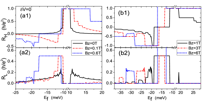
Figure 4: (Color online) Hall resistance $R_{H}$ and longitudinal resistance $R_{L}$ as a function of Fermi energy with fixed magnetic field $B_{z}$. $\delta V=0$, $m_{0}/B<0$.

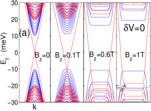
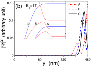
Figure 5: (Color online) (a) The energy dispersion for a 1D nanoribbon with width of 480 nm for several magnetic field respectively. (b) Wave function distribution along $y$ direction for the exotic edge states, (A,B) and edge state due to LL, C. Inset of (b) is the amplification of (a). Parameters are identical to those in Fig.4.

IV Transport analysis

This section is to study the transport properties of a standard Hall bar with six leads (as shown in the inset of Fig.3) by Landauer-Büttiker formalism at zero temperature. On one hand numerical results here will verify the analysis in Sec.II and Sec.III. On the other hand finite size will lead to an intrinsic edge state due to inverted energy band in the nontrivial energy gap. And in presence of magnetic field, this intrinsic edge state will coexist or couple with the magnetic edge state due to LLs leading to exotic transport phenomena.

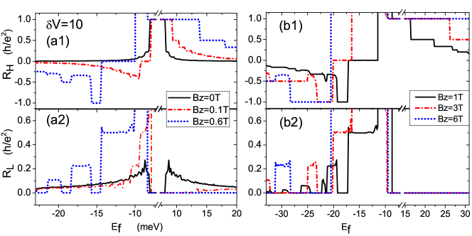
Figure 6: (Color online) (a,b) Hall resistance $R_{H}$ and longitudinal resistance $R_{L}$ as a function of Fermi energy with fixed magnetic field $B_{z}$. $\delta V=10meV$, $m_{0}/B<0$.

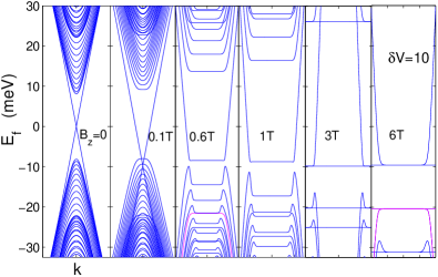
Figure 7: (Color online) The energy dispersion for a nanoribbon with width of 480 nm for several magnetic field. Parameters are identical to those in Fig.6.

For convenience, we discretize the Hamiltonian in Eq.(8) in square lattice:

$$H_{d} = \sum_{\mathbb{x}}[\psi^{\dagger}_{\mathbb{x}}T_{0}\psi_{\mathbb{x}}+(\psi^{\dagger}_{\mathbb{x}}T_{x}\psi_{\mathbb{x}+\delta\hat{x}}+\psi^{\dagger}_{\mathbb{x}}T_{y}\psi_{\mathbb{x}+\delta\hat{y}}+H.C.)]$$

$$T_{0} = M\sigma_{z}+\tilde{m}_{0}\tau_{x}+\frac{\delta V}{2}\tau_{z}$$

$$T_{x} = (it_{a}\sigma_{y}\tau_{z}-B_{a}\tau_{x})e^{i\phi_{{\mathbb{x},\mathbb{x}+\delta\hat{x}}}}$$

$$T_{y} = (-it_{a}\sigma_{x}\tau_{z}-B_{a}\tau_{x})e^{i\phi_{{\mathbb{x},\mathbb{x}+\delta\hat{y}}}}$$ (19)

where $\mathbb{x}$ is the site index and $\delta\hat{x}\,(\delta\hat{y})$ is the unit vector along $x\,(y)$ direction. $\psi_{\mathbb{x}}=(a_{\mathbb{x}},b_{\mathbb{x}},c_{\mathbb{x}},d_{\mathbb{x}})^{T}$ represents the four operators annihilate an electron on site ${\mathbb{x}}$ in states $|t\uparrow\rangle,\,|t\downarrow\rangle,|b\uparrow\rangle,\,|b\downarrow\rangle$ respectively. $V$ represents the onsite energy term and $T_{x/y}$ represents the hopping term along $x/y$ direction. The effect of the perpendicular magnetic field $B_{z}$ is included by adding to the hopping matrix a phase term $\phi_{\mathbb{x}_{1},\mathbb{x}_{2}}=\int_{\mathbb{x}_{1}}^{\mathbb{x}_{2}}\mathbb{A}\cdot d\mathbb{l}/\phi_{0}$ where $\mathbb{A}=(B_{z}y,0,0)$ is the vector potential inducing magnetic field $-B_{z}$ along $z$ direction and $\phi_{0}=\hbar/e$. Other parameters in Hamiltonian (IV) are given as : $t_{a}=\frac{\hbar v_{F}}{2a}$, $B_{a}=B/a^{2}$, $\tilde{m}_{0}=m_{0}+4B_{a}$. $a=4nm$ is the lattice constant along x/y direction. The width of both the central region and six contacts is $480nm$.

In Landauer-Büttiker formalism the current flowing out of lead $i$ is given by,LBformula ; long1 ; sun1

$$I_{i}=\frac{e^{2}}{h}\sum_{j}T_{ij}(E_{f})(V_{i}-V_{j})$$ (20)

where $V_{i}$ is the bias voltage on lead $i$ and $T_{ij}(E_{f})=Tr[\Gamma^{i}G^{r}\Gamma^{j}G^{a}]$ is the transition coefficient from lead $j$ to $i$ at Fermi energy $E_{f}$. $G^{r}=[G^{a}]^{\dagger}=1/(E_{f}-\tilde{H}-\sum_{i=1}^{6}\Sigma_{i}^{r})$ is the retarded Green’s functions and $\tilde{H}$ is the Hamiltonian of the central region. $\Sigma_{i}^{r}=[\Sigma_{i}^{a}]^{\dagger}$ is the retarded self-energy coupling to lead $i$ which can be calculated numerically.DHLsgf The linewidth function $\Gamma_{i}$ is related to the self-energy by $\Gamma_{i}=i(\Sigma_{i}^{r}-\Sigma_{i}^{a})$. We apply a small bias $V=V_{1}-V_{4}$ across the sample and set leads $2,3,5,6$ as voltage leads with current being zero. Then from Eq.(20), voltages $V_{2}$, $V_{3}$, $V_{5}$ and $V_{6}$ and the current $I=I_{1}=-I_{4}$ flowing over the sample from lead $1$ to $4$ can be calculated. At last the Hall and longitudinal resistance are given by $R_{H}\equiv\frac{V_{6}-V_{2}}{I}$ and $R_{L}\equiv\frac{V_{2}-V_{3}}{I}$ respectively.

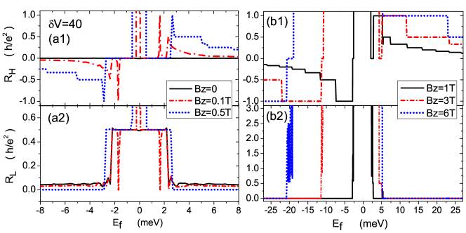
Figure 8: (Color online) (a,b) Hall resistance $R_{H}$ and longitudinal resistance $R_{L}$ as a function of Fermi energy with fixed magnetic field $B_{z}$. $\delta V=40meV,\,m_{0}/B<0$.

Figure 9: (Color online) The energy dispersion for a nanoribbon with width of 480 nm for several magnetic field. Parameters are identical to those in Fig.8.

The longitudinal and Hall resistances in absence of magnetic field are shown in Fig.3, which verify the analysis in Sec.II. Fig.3(a1-2) correspond to the $m_{0}/B<0$ case. For $\delta V<2\sqrt{M^{2}-m_{0}^{2}}\approx 28meV$, Hall resistance shows a Hall plateau with the plateau value $h/e^{2}$ and the longitudinal resistance is zero at the position of the Hall plateau. This corresponds to the QAH phase which has been observed in the recent experiment.Xue_QAH For $28mev<\delta V<\sqrt{M^{2}-m_{0}\hbar^{2}v_{F}^{2}/|B|}\approx 56mev$, the Hall resistance is almost zero, but the longitudinal resistance shows a plateau with the plateau value $h/2e^{2}$, which corresponds to the QPH phase, i.e. the phase IV in Fig.1(a1). Increase $\delta V$ anymore, the resistance at certain regime become infinite corresponding to the normal-insulator phase VII in Fig.1(a1). On the other hand, for $m_{0}/B>0$ case, the system directly goes from the QAH phase to the normal-insulator phase without passing the QPH phase by increasing $\delta V$. Therefore there is no longitudinal resistance plateau, and only the Hall plateau is observed at $\delta V<2\sqrt{M^{2}-m_{0}^{2}}$ (see Fig.3(b1-2)). $R_{H}$ and $R_{L}$ are symmetric about $E_{f}=0$. The reason is that the Hamiltonian (see Eq.(8)) is invariant under the spatial inversion and electron-hole transformation and resultantly the energy band (see Fig.1(a4,b4)) is symmetric about $E_{f}=0$. Magnetic field will destroy electron-hole symmetry and the energy band and resistances will be asymmetric about $E_{f}=0$ as shown in the following.

In the following we study the effect of magnetic field. We first consider the case $m_{0}/B<0$ and $\delta V=0$. The longitudinal and Hall resistances are shown in Fig.4. For positive Fermi energy, there are several integer quantum Hall (IQH) -like plateaus with zero longitudinal resistance and integer Hall resistance. These plateaus are consistent with Chern numbers calculated by Kubo formula and can be explained with LL spectrum completely. For negative Fermi energy at small magnetic field, see Fig.4(a), there is no IQH-like plateau but some exotic plateaus with nonzero longitudinal resistances. However both IQH-like and exotic plateaus will form at negative Fermi energy regime for larger magnetic field, see Fig.4(b). The exotic plateaus with values $(R_{L},\,R_{H})=(\frac{1}{2}h/e^{2},0),\,(\frac{2}{9}h/e^{2},-\frac{1}{3}h/e^{2}),\,(\frac{3}{28}h/e^{2},-\frac{2}{7}h/e^{2})...$, can be described by

$$R_{L}=\frac{n_{a}n_{c}}{n^{3}_{a}+n_{c}^{3}}\frac{h}{e^{2}},\,\,R_{H}=\frac{n_{a}^{2}-n_{c}^{2}}{n^{3}_{a}+n_{c}^{3}}\frac{h}{e^{2}},$$ (21)

with $(n_{a},\,n_{c})=(1,1),\,(1,2),\,(1,3)...$ . The first pair is a QSH-like plateau and the followings are fractional plateaus. $n_{c}$ and $n_{a}$ represent the number of clockwise and anticlockwise edge states respectively. Suppose that only edge states contribute to transport without mixing, then Eq.(21) can be derived straightforwardly with Landauer-Büttiker formula similar with that in the QSH effect case.PRB_HgTe(J.C.Chen) Therefore these exotic plateaus originate from the coexistence of clockwise and anticlockwise edge states.

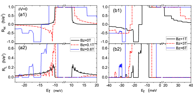
Figure 10: (Color online) (a,b) Hall resistance $R_{H}$ and longitudinal resistance $R_{L}$ as a function of Fermi energy with fixed magnetic field $B_{z}$. $\delta V=0$, $m_{0}/B>0$.

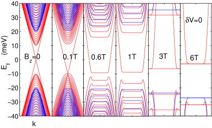
Figure 11: (Color online) The energy dispersion for a nanoribbon with width of 480 nm for several magnetic field. Parameters are identical to those in Fig.10.

In order to examine it more clearly, we study the energy dispersion for several magnetic fields as shown in Fig.5(a). Since $\delta V=0$ the Hamiltonian can be decoupled into inverted (see red curves in Fig.5(a)) and non-inverted (see blue curves in Fig.5(a)) block. Increasing magnetic field the Dirac cone will move downward into the trivial band. Then magnetic edge states due to LLs and the intrinsic edge state due to intrinsic energy band will counterpropagate at the same edge of the sample for certain Fermi energy regime. Consequently a nonzero longitudinal plateau will emerge. Such analysis is consistent with that by LL spectrum in Fig.2(a1).

According to Fig.2(a1) the first fractional plateau will only exist below a critical magnetic field about $0.7T$, where the zero mode $E_{0-}$ with positive Chern number cross with the $N=1$ mode of the inner hole-like LLs with negative Chern number. The critical values for the other fractional plateaus are smaller. However Fig.4(b) shows that exotic plateaus can survive even above the critical value but become less perfect. And they can exist even for $E_{f}<-20meV$ while the phase with counterpropagate edge states suggested in Fig.2(a1) lies between $-20meV<E_{f}<-10meV$. The reason is that large enough magnetic field will move the Dirac cone into the nontrivial band. And these two kinds of edge states will couple to form an exotic energy band with two humps connected to the LL and its edge state, as shown in Fig.5(a) and the inset of Fig.5(b). From Fig.2(a1), the Chern number in the region $E_{f}=-21meV$ and $B_{z}=1T$ (see the green line in Fig.5(a) or inset of Fig.5(b)) is equal to $-1$, and there should be only a hole edge state (the state C, see inset of Fig.5(b)). However, due to the exotic band with two humps, a pair of extra counterpropagate edge states (states A and B) at one edge of the sample emerge. Fig.5(b) gives the distribution of the wave functions of these extra states A, B and the hole edge state C, and they are indeed edge states. Therefore, the clockwise and anticlockwise edge states number is $(n_{a},n_{c})=(1,2)$ to give rise to the first fractional plateau $(R_{L}\,,R_{H})=(\frac{2}{9}h/e^{2},-\frac{1}{3}h/e^{2})$, although the Chern number is $-1$ as shown in Fig.2(a1).

The perfect QSH-like plateau $(R_{L},\,R_{H})=(\frac{1}{2}h/e^{2},\,0)$ is consistent with the QSH-like phase suggested in Fig.2(a1) (see the region with Chern number 0). But unlike the QSH effect, counterpropagating edge states here are caused by magnetic field with time reversal symmetry broken. The width of this plateau increases to a maximum at $B_{z}=0.7T$ and then decreases as the magnetic field $B_{z}$ increases. It will disappear if the magnetic field is larger than the critical value $B_{c}=-\frac{\hbar m_{0}}{eB}\approx 4.1T$.

Then we consider the case with SIA potential $\delta V$ but still in the QAH phase with $m_{0}/B<0,\,\delta V=10meV$. Fig.6 and Fig.7 show the longitudinal and Hall resistance and the energy dispersion, respectively. The inner (outer) bulk bands are nontrivial (trivial). Moderate magnetic field can move the Dirac cone into the nontrivial band to form the exotic energy band with two humps accompanied by an insulator energy gap. The resistance will be infinite in the gap region, see Fig.6. On the right side of the gap is the QAH plateau and other IQH-like plateaus consistent with the LL spectrum. On the left side of the gap is the IQH-like and exotic plateaus. Comparing energy dispersion in Fig.7 and LL spectrum in Fig.2(a2), we find that hole-like bands corresponding to the non-trivial branch form obvious humps while those corresponding to the trivial branch don’t. It indicates that the coupling between intrinsic edge state and trivial band is weaker than that to the nontrivial band, since the intrinsic edge state is due to the nontrivial band. Increasing magnetic field, hole-like LLs move downward except $E_{0-}$ (pink line in Fig.7) which will move upward below about $B_{c}=4.1T$, see Fig.2(a2). For large enough magnetic field, $E_{0-}$ will be the first hole-like LL without humps to vanish the imperfect QSH-like plateau. But the first fractional plateau will remain since the second hole-like LL corresponds to the nontrivial band, see Fig.2(a2).

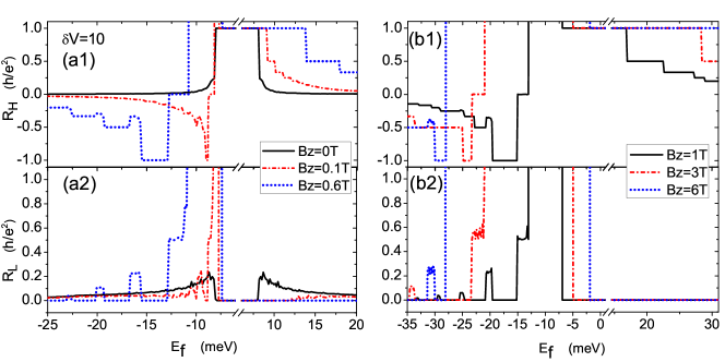
Figure 12: (Color online) (a,b) Hall resistance $R_{H}$ and longitudinal resistance $R_{L}$ as a function of Fermi energy with fixed magnetic field $B_{z}$. $\delta V=10meV$, $m_{0}/B>0$.

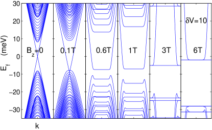
Figure 13: (Color online) The energy dispersion for a nanoribbon with width of 480 nm for several magnetic field. Parameters are identical to those in Fig.12.

In the following, the influence of magnetic field on QPH phase is studied with SIA potential $\delta V=40\,meV$. Fig.8 show the longitudinal and Hall resistance and Fig.9 is the energy band. Magnetic field moves two Dirac cones upward and downward respectively to split the degeneracy. Therefore there will be exotic plateaus for both negative and positive Fermi energy regime. But unlike the QAH phase the intrinsic edge state can not enter inside the bulk bands, see as Fig.7 and Fig.9. Therefore, only the two innermost LL edge states can couple with the intrinsic edge state and form the exotic band with two humps, which cause the QSH-like plateau with the longitudinal resistance $h/2e^{2}$ and zero Hall resistance at small magnetic field. The third and following exotic plateaus will not appear. Increase the magnetic field, two humps gradually fall and the QSH-like plateau disappear. At the large magnetic field, the system come into the IQH regime, in which the quantum Hall plateaus with the plateau value $h/ne^{2}$ ($n=\pm 1,\pm 2,...$) well form on both the electron- and hole-sides and the longitudinal resistance is zero, see Fig.8(b).

Finally, the case $m_{0}/B>0$ is studied. Only the QAH phase is considered, since in trivial phase only IQH-like plateaus appear which can be described by LL spectrum completely. Resistance curves for $\delta V=0$ and $\delta V=10meV$ are shown in Figs. 10 and 12. And they can be understood following the analysis for $m_{0}/B<0$ with the energy dispersion (Figs.11 and 13) and LL spectrum (Fig.2(b1-2)). The exotic plateau may be successive for $\delta V=0$, see Fig.10(b), but separated by a IQH-like plateau if $\delta V\neq 0$, see Fig.12(b), similar with that in the case $m_{0}/B<0$. But unlike $m_{0}/B<0$, the inner (outer) bands are nontrivial (trivial) whether SIA potential vanishes or not. Therefore exotic plateaus are imperfect even for $\delta V=0$.

To extensively show the effect of SIA potential, the phase diagram at $B_{z}=3T$ is plotted in Fig.14. Integers show the Hall conductance ($G_{H}=\frac{R_{H}}{R_{H}^{2}+R_{L}^{2}}$) of the region with zero longitudinal component ($G_{L}=\frac{R_{L}}{R_{H}^{2}+R_{L}^{2}}$) which are consistent with Fig.2(a5,b5). Light green regions are due to the formation of exotic bands and show the region where the longitudinal resistance doesn’t vanish. They occupy the QH phase region partially and narrow the insulator gap. The area of light green region is much smaller for $m_{0}/B>0$ comparing with that for $m_{0}/B<0$. For large enough $\delta V$, the light green region will disappear since $\delta V$ leads to the normal-insulator phase.

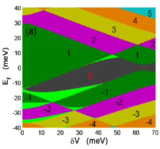
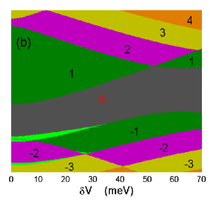
Figure 14: (Color online) Phase diagram at $B_{z}=3T$ in the plane of Fermi energy and SIA potential for (a) $m_{0}/B<0$ and (b) $m_{0}/B>0$ respectively. Integers show the Hall conductance of the region with zero longitudinal component. Exotic plateaus with nonzero longitudinal component form in the light green region.

V Conclusion

In summary we have studied the effect of magnetic field on an ultrathin magnetic topological insulator film with structure inversion asymmetry term. We give the phase diagram in the plane of the structure-inversion-asymmetry strength and the Fermi energy and derive the Landau level spectrum analytically. We find that the quantum anomalous Hall phase will survive increasing magnetic field. A new QSH-like phase will form at moderate magnetic field. Transport properties is simulated in Landauer-Büttiker formalism. Exotic resistance plateau with nonzero longitudinal elements are predicted in a standard Hall bar. Additionally, the effect of structure inversion asymmetry term on Landau level spectrum and transport behavior is investigated in detail.

References

- (1) K. v. Klizing, G. Dorda, and M. Pepper, Phys.Rev.Lett 45, 494 (1980).
- (2) E. H. Hall, Am.J.Math. 2, 287 (1879).
- (3) F. D. M. Haldane, Phys. Rev. Lett. 61,2015 (1988).
- (4) R. Yu, W. Zhang, H. J. Zhang, S. C. Zhang, X. Dai, and Z. Fang, Science 329, 61 (2010).
- (5) M. Onoda and N. Nagaosa, Phys. Rev. Lett. 90, 206601 (2003); X. L. Qi, Y. S. Wu, and S. C. Zhang, Phys. Rev. B 74, 085308 (2006); X. L. Qi, T. L. Hughes, and S. C. Zhang, Phys.Rev.B 78, 195424 (2008); C. X. Liu, X. L. Qi, X. Dai, Z. Fang, and S. C. Zhang, Phys. Rev. Lett. 101, 146802 (2008); Z. Qiao, S. A. Yang, W. X Feng, W. K Tse, J. Ding, Y. G Yao, J. Wang, and Q. Niu, Phys.Rev.B 82, 161414 (2010); K. Nomura, and N. Nagaosa, Phys.Rev.Lett. 106, 166802 (2011); H. Jiang, Z. H. Qiao, H. W. Liu, and Q. Niu, Phys.Rev.B 85, 045445 (2012); W. K. Tse, Z. H. Qiao, Y. G. Yao, A. H. MacDonald, and Q. Niu, Phys.Rev.B 83, 155447 (2011); T. W. Chen, Z. R. Xiao, D. W. Chiou, and G. Y. Guo, Phys.Rev.B 84, 165453 (2011); J. Ding, Z. H. Qiao, W. X. Feng, Y. G. Yao, and Q. Niu, Phys.Rev.B 84, 195444 (2011).
- (6) E. H. Hall, Philos. Mag. 12, 157 (1881); N. Nagaosa, J. Sinova, S. Onoda, A. H. MacDonald, and N. P. Ong, Rev. Mod. Phys. 82 1539 (2010).
- (7) C. L. Kane, E. J. Mele, Phys. Rev. Lett. 95, 146802 (2005); B. A. Bernevig and S. C. Zhang, Phys. Rev. Lett. 96, 106802 (2006); B. A. Bernevig, T. L. Hughes and S. C. Zhang, Science 314, 1757 (2006).
- (8) M.I. Dyakonov and V.I. Perel, Sov. Phys. JETP Lett. 13, 467 (1971); J. E. Hirsch, Phys. Rev. Lett. 83, 1834 (1999); Y. K. Kato, R. C. Myers, A. C. Gossard, D. D. Awschalom, Science 306, 1910 (2004).
- (9) M. König, S. Wiedmann, C. Brüne, A. Roth, H. Buhmann, L. W. Molenkamp, X. L Qi, and S. C. Zhang, Science 318, 766 (2007).
- (10) H. Jiang, S. Cheng, Q.-F. Sun, and X. C. Xie, Phys. Rev. Lett. 103, 036803 (2009).
- (11) C. Z. Chang, J. S. Zhang, X. Feng, J. Shen, Z. C. Zhang, M. H. Guo, K. Li, Y. B. Ou, P. Wei, L. L. Wang, Z. Q. Ji, Y. Feng, S. H. Ji, X. Chen, J. F. Jia, X. Dai, Z. Fang, S. C. Zhang, K. He, Y. Y. Wang, L. Lu, X. C. Ma, and Q. K. Xue, Science 340, 167 (2013).
- (12) M. Z. Hasan and C. L. Kane, Rev. Mod. Phys. 82, 3045 (2010); X. L. Qi, S. C. Zhang, Rev. Mod. Phys. 83, 1057 (2011).
- (13) W. Y. Shan, H. Z. Lu, and S. Q. Shen, New J. Phys. 12, 043048 (2010).
- (14) H. Z. Lu, W. Y. Shan, W. Yao, Q. Niu, and S. Q. Shen Phys. Rev. B 81, 115407 (2010); H. C. Li, L. Sheng, D. N. Sheng, and D. Y. Xing Phys. Rev. B 82, 165104 (2010).
- (15) A. A. Zyuzin and A. A. Burkov, Phys. Rev. B 83 195413 (2011).
- (16) H. C. Li, L. Sheng, and D. Y. Xing Phys. Rev. B 84, 035310 (2011).
- (17) C. X. Liu, X. L. Qi, H. J. Zhang, X. Dai, Z. Fang, and S. C. Zhang, Phys. Rev. B 82, 045122 (2010).
- (18) M. Tahir, K. Sabeeh, and U. Schwingenschlögl, J. Appl. Phys. 113, 043720 (2013).
- (19) A. I. Akheizer and V. B. Berestetsky, (Interscience, New York, 1965).
- (20) P. Cheng, C. l. Song, T. Zhang, Y. Y. Zhang, Y. L. Wang, J. F. Jia, J. Wang, Y. Y. Wang, B. F. Zhu, X. Chen, X. C. Ma, K. He, L. L. Wang, X. Dai, Z. Fang, X. C. Xie, X. L. Qi, C. X. Liu, S. C. Zhang, and Q. K. Xue, Phys.Rev.Lett 105, 076801 (2010); T. Hanaguri, K. Igarashi, M. Kawamura, H. Takagi, and T. Sasagawa, Phys. Rev. B 82, 081305 (2010); B. Sacepe, J. B. Oostinga, J. Li, A. Ubaldini, N. J. G. Couto, E. Giannini, and A. F. Morpurgo, Nature Commun. 2, 575 (2011).
- (21) Y. P Jiang, Y. L. Wang, M. Chen, Z. Li, C. L. Song, K. He, L. L. Wang, X. Chen, X. C. Ma, and Q. K. Xue, Phys. Rev. Lett 108, 016401 (2012).
- (22) Y. Okada, W. W. Zhou, C. Dhital, D. Walkup, Y. Ran, Z. Wang, S. D. Wilson, and V. Madhavan, Phys. Rev. Lett 109, 166407 (2012).
- (23) C. Brüne, C. X. Liu, E. G. Novik, E. M. Hankiewicz, H. Buhmann, Y. L. Chen, X. L. Qi, Z. X. Shen, S. C. Zhang, and L. W. Molenkamp, Phys.Rev.Lett 106, 126803 (2011).
- (24) H. Z Lu, A. Zhao, and S. Q Shen, Phys. Rev. Lett 111, 146802 (2013).
- (25) H. J. Zhang, C. X. Liu, X. L. Qi, X. Dai, Z. Fang, and S. C. Zhang, Nat. Phys. 5, 438 (2009).
- (26) Parameters given as: , , , and . and are the eigenvectors of Hamiltonian at point, and are the corresponding eigenvalues. See Ref.(NJP(Shan) ) for detail of derivation.
- (27) C. X. Liu, H. J. Zhang, B. H. Yan, X. L. Qi, T. Frauenheim, X. Dai, Z. Fang, and S. C. Zhang, Phys. Rev. B 81, 041307(R) (2010).
- (28) H. C. Li, L. Sheng, and D. Y. Xing, Phys. Rev. B 85, 045118 (2012).
- (29) Y. Zhang, K. He, C.-Z. Chang, C.-L. Song, L.-L. Wang, X. Chen, J.-F. Jia, Z. Fang, X. Dai, W.-Y. Shan, S. -Q. Shen, Q. Niu, X. -L. Qi, S. -C. Zhang, X. -C. Ma, and Q. -K Xue, Nat. Phys. 6, 584 (2010).
- (30) J. C. Chen, J. Wang, and Q. F. Sun, Phys. Rev. B 85, 125401 (2012).
- (31) H. Jiang, L. Wang, Q.-F. Sun, and X. C. Xie, Phys. Rev. B 80, 165316 (2009).
- (32) D. J. Thouless, M. Kohmoto, M. P. Nightingale, and M. D. Nijs, Phys. Rev. Lett. 49, 405 (1982); M. Kohmoto, Ann. Phys. (NY) 160, 343 (1985).
- (33) Chern number is calculated directly with Eq.(10) in the discrete k-space with discretized Hamiltonian given in Eq.(IV). We find it is accurate enough to discretize the first Brillouin zone up to lattice points. For each k mesh the Hamiltonian is . in the absence of magnetic field and satisfies and with the presence of magnetic field.
- (34) S. Q. Shen, M. Ma, X. C. Xie, and F. C. Zhang, Phys. Rev. Lett 92, 256603 (2004).
- (35) V. P. Gusynin and S. G. Sharapov, Phys. Rev. Lett 95, 146801 (2005).
- (36) K. S. Novoselov, A. K. Geim, S. V. Morozov, D. Jiang, M. I. Katsnelson, I. V. Grigorieva, S. V. Dubonos, and A. A. Firsov, Nature (London) 438, 197 (2005). Y. Zhang, Y.-W. Tan, H. L. Stormer, and P. Kim, Nature (London) 438, 201 (2005).
- (37) S. Datta, ( Cambridge University Press, Cambridge, England, 1995 ).
- (38) W. Long, Q.-F. Sun, and J. Wang, Phys. Rev. Lett. 101, 166806 (2008).
- (39) Q.-F. Sun and X. C. Xie, Phys. Rev. Lett. 104, 066805 (2010).
- (40) D. H. Lee and J. D. Joannopoulos, Phys. Rev. B 23, 4997 (1981); M. P. L. Sancho, J. M. L. Sancho, and J. Rubio, J. Phys. F 15, 851 (1985).