Popular Conjectures as a Barrier for
Dynamic Planar Graph Algorithms

Abstract

The dynamic shortest paths problem on planar graphs asks us to preprocess a planar graph $G$ such that we may support insertions and deletions of edges in $G$ as well as distance queries between any two nodes $u,v$ subject to the constraint that the graph remains planar at all times. This problem has been extensively studied in both the theory and experimental communities over the past decades and gets solved millions of times every day by companies like Google, Microsoft, and Uber. The best known algorithm performs queries and updates in $\tilde{O}({n^{2/3}})$ time, based on ideas of a seminal paper by Fakcharoenphol and Rao [FOCS’01]. A $(1+\varepsilon)$-approximation algorithm of Abraham et al. [STOC’12] performs updates and queries in $\tilde{O}({\sqrt{n}})$ time. An algorithm with a more practical $O(\operatorname{poly}\log{n})$ runtime would be a major breakthrough. However, such runtimes are only known for a $(1+\varepsilon)$-approximation in a model where only restricted weight updates are allowed due to Abraham et al. [SODA’16], or for easier problems like connectivity.

In this paper, we follow a recent and very active line of work on showing lower bounds for polynomial time problems based on popular conjectures, obtaining the first such results for natural problems in planar graphs. Such results were previously out of reach due to the highly non-planar nature of known reductions and the impossibility of “planarizing gadgets”. We introduce a new framework which is inspired by techniques from the literatures on distance labelling schemes and on parameterized complexity.

Using our framework, we show that no algorithm for dynamic shortest paths or maximum weight bipartite matching in planar graphs can support both updates and queries in amortized $O(n^{\frac{1}{2}-\varepsilon})$ time, for $\varepsilon>0$, unless the classical all-pairs-shortest-paths problem can be solved in truly subcubic time, which is widely believed to be impossible. We extend these results to obtain strong lower bounds for other related problems as well as for possible trade-offs between query and update time. Interestingly, our lower bounds hold even in very restrictive models where only weight updates are allowed.

1 Introduction

The dynamic shortest paths problem on planar graphs is to preprocess a planar graph $G$, e.g. the national road network, so that we are able to efficiently support the following two operations:

• At any point, we might insert or remove an edge $(u,v)$ in $G$, e.g. in case a road gets congested due to an accident. Such updates are subjected to the constraint that the planarity of the graph is not violated. We may also consider another natural variant in which we are only allowed to update the weights of existing edges.

• We want to be able to quickly answer queries that ask for the length of the shortest path between two given nodes $u$ and $v$, in the most current graph $G$.

This is a problem that gets solved millions of times every day by companies like Google, Microsoft, and Uber on graphs such as road networks with many millions of nodes. It is thus a very important question in both theory and practice whether there exists data structures that can perform updates and (especially) queries on graphs with $n$ nodes in polylogarithmic or even $n^{o(1)}$ time.

Shortest paths problems on planar graphs provide an ideal combination of mathematical simplicity and elegance with faithful modeling of realistic applications of major industrial interest. The literature on the topic is too massive for us to survey in this paper: the current draft of the book “Optimization Problems in Planar Graphs” by Klein and Mozes [42] dedicates four chapters to the algorithmic techniques for shortest paths by the theory community. While near-optimal algorithms are known for most variants of shortest paths on static planar graphs, the dynamic setting has proven much more challenging.

Since an $s,t$-shortest path in a planar graph can be found in near-linear time (linear time for non-negative weights) [39, 28], there is a naïve algorithm for the dynamic problem that spends $\tilde{O}(n)$ time on queries. After progress on other related problems on dynamic planar graphs [29, 30, 24, 31, 61, 44, 39], the first sublinear bound was obtained in the seminal paper of Fakcharoenphol and Rao [28], which introduced new techniques that led to major results for other problems like Max Flow (even on static graphs) [17, 47]. The amortized time per operation was $O(n^{2/3}\log^{7/3}n)$ and $O(n^{4/5}\log^{13/5}n)$ if negative edges are allowed, and follow up works of Klein [43], Italiano et al. [40], and Kaplan et al. [41] reduced the runtime to $O(n^{2/3}\log^{5/3}n)$ (even allowing negative weights), and most recently, Gawrychowski and Karczmarz [33] reduced it further to $O(n^{2/3}\frac{\log^{5/3}n}{\log^{4/3}\log{n}})$. In fact these algorithms give a trade-off on the update and query time of $\tilde{O}({n/\sqrt{r}})$ and $\tilde{O}({r})$, for all $r$. The problem has also been extensively studied from an engineering viewpoint on real-world transportation networks (see [21] for a survey). State of the art algorithms [13, 20, 22, 34, 60] are able to exploit further structure of road networks (beyond planarity) and process updates to networks with tens of millions of nodes in milliseconds.

In a recent SODA’16 paper, Abraham et al. [6] study worst case bounds under a restricted but realistic model of dynamic updates in which a base graph $G$ is given and one is allowed to perform only weight updates subject to the following constraint: For any updated graph $G^{\prime}$ it must hold that $d_{G}(u,v)\leq d_{G^{\prime}}(u,v)\leq M\cdot d_{G}(u,v)$ for all $u,v$ and some parameter $M$. (Note that this will hold if, for example, the weight of each edge only changes to within a factor of $M$.) In this model, the authors obtain a $(1+\varepsilon)$-approximation algorithm that maintains updates in $O(\operatorname{poly}\log{n}\cdot M^{4}/\varepsilon^{3})$ time. Without this restriction, the best known $(1+\varepsilon)$-approximation algorithms use $\tilde{O}(\sqrt{n})$ updates [44, 7]. Thus, when $M$ is small, this model allows for a major improvement over the above results which require polynomial time updates. But is it enough to allow for exact algorithms with subpolynomial updates? Such a result would explain the impressive experimental performance of state of the art algorithms.

On the negative side, Eppstein showed that $\Omega(\log n/\log\log n)$ time is required in the cell probe model [27] for planar connectivity (and therefore also shortest path). However, an unconditional $\log^{\omega(1)}{n}$ lower bound is far beyond the scope of current techniques (see [18]). In recent years, much stronger lower bounds were obtained for dynamic problems under certain popular conjectures [57, 54, 3, 46, 38, 5, 19]. For example, Roditty and Zwick [57] proved an $n^{2-o(1)}$ lower bound for dynamic single source shortest paths in general graphs under the following conjecture.

Conjecture 1 (APSP Conjecture).

There exists no algorithm for solving the all pairs shortest paths (APSP) problem in general weighted (static) graphs in time $O(n^{3-\varepsilon})$ for any $\varepsilon>0$.

However, the reductions used in these results produce graphs that are fundamentally non-planar, such as dense graphs on three layers, and popular approaches for making them planar, e.g. by replacing each edge crossing with a small “planarizing gadget”, are provably impossible (this was recently shown for matching [36] and is easier to show for problems like reachability and shortest paths). Due to this and other challenges no (conditional) polynomial lower bounds were known for any natural problem on (static or dynamic) planar graphs.

On a more general note, an important direction for future research on the fine-grained complexity of polynomial time problems (a.k.a. Hardness in P) is to understand the complexity of fundamental problems on restricted but realistic classes of inputs. A Recent result along these lines is the observation that the $n^{2-o(1)}$ lower bound for computing the diameter of a sparse graph [56] holds even when the treewidth of the graph is $O(\log{n})$ [4]. In this paper, we take a substantial step in this direction, proving the first strong (conditional) lower bounds for natural problems on planar graphs.

1.1 Our Results

We present the first conditional lower bounds for natural problems on planar graphs using a new framework based on several ideas for conditional lower bounds on dynamic graphs combined with ideas from parameterized complexity [50, 51] and labeling schemes [32]. We believe that this framework is of general interest and might lead to more interesting results for planar graphs. Our framework shows an interesting connection between dynamic problems and distance labeling and also slightly improves the result of [32] providing a tight lower bound for distance labeling in weighted planar graphs (this is discussed in Section 1.2).

Our first result is a conditional polynomial lower bound for dynamic shortest paths on planar graphs. Like several recent results [64, 2, 1, 5, 58, 19], our lower bound is based on the APSP conjecture. Perhaps the best argument for this conjecture is the fact that it has endured decades of extensive algorithmic attacks. Moreover, due to the known subcubic equivalences [64, 1, 58], the conjecture is false if and only if several other fundamental graph and matrix problems can be solved substantially faster.

Theorem 1.

No algorithm can solve the dynamic APSP problem in planar graphs on $N$ nodes with amortized query time $q(N)$ and update time $u(N)$ such that $q(N)\cdot u(N)=O(N^{1-\varepsilon})$ for any $\varepsilon>0$ unless Conjecture 1 is false. This holds even if we only allow weight updates to $G$.

Thus, under the APSP conjecture, there is no hope for a very efficient dynamic shortest paths algorithm on planar graphs with provable guarantees. We show that an algorithm achieving $O(n^{1/2-\varepsilon})$ time for both updates and queries is unlikely, implying that the current upper bounds achieving $\tilde{O}(n^{2/3})$ time are not too far from being conditionally optimal. Furthermore, our result implies that any algorithm with subpolynomial query time must have linear update time (and the other way around). Thus, the naïve algorithm of simply computing the entire shortest path every time a query is made is (conditionally) optimal if we want $n^{o(1)}$ update time.

An important property of Theorem 1 is that our reduction does not even violate planarity with respect to a fixed embedding. Thus, we give lower bounds even for plane graph problems, which in many cases allow for improved upper bounds over flexible planar graphs (e.g. for reachability[23, 11]). Moreover, our graphs are grid graphs which are subgraphs of the infinite grid, a special and highly structured subclass of planar graphs. Finally, as stated in Theorem 1 our lower bound holds even for the edge weight update model of Abraham et al. [6], where each edge only ever changes its weight to within a factor of $M>1$. While they obtain fast $\operatorname{polylog}(n)$ time $(1+\varepsilon)$-approximation algorithm in this model, we show that an exact answer with the same query time likely requires linear update time and that an algorithm with $O(n^{1/2-\varepsilon})$ runtime for both is highly unlikely. Thus, further theoretical restrictions need to be added in order to explain the impressive performance on real road networks.

We also extend Theorem 1 to the case in which we only need to maintain one $s,t$ distance (the $s,t$-shortest path problem). While this problem is equivalent to the APSP version in general (as we may connect $s$ and $t$ to any two nodes $u,v$ we wish to know the distance between) this may violate planarity and especially a fixed embedding. We show that this problem exhibits similar trade-offs under Conjecture 1 even if we are only allowed to update weights. Finally, we note that in the case of directed planar graphs allowing negative edge weights our techniques can be extended to show the same hardness result for any approximation under Conjecture 1.

Next, we seek a lower bound for the unweighted version of the problem, which arguably, is of more fundamental interest. Typically, a conditional lower bound under the APSP conjecture for a weighted problem can be modified into a lower bound for its unweighted version under the Boolean Matrix Multiplication (BMM) Conjecture [25, 57, 64, 3, 1]. While for combinatorial algorithms the complexity of BMM is conjectured to be cubic, it is known that using algebraic techniques there is an $O(n^{\omega})$ algorithm, where $\omega<2.373$ [63, 49]. When reducing to dynamic problems, however, lower bounds under BMM are often under a certain online version of BMM for which, Henzinger et al. [38] conjecture that there is no truly subcubic algorithms, even using algebraic techniques. This Online Matrix Vector Multiplication (OMv) Conjecture is stated formally in Section 5.

The OMv conjecture implies strong lower bounds for many dynamic problems on general graphs [38], via extremely simple reductions [3, 38]. Our next result is a significantly more involved reduction from OMv to dynamic shortest paths on planar graphs, giving unweighted versions of the theorems above. The lower bounds are slightly weaker but they still rule out algorithms with subpolynomial update and query times, even in grid graphs. We remark that all lower bounds under the APSP conjecture in this paper, such as Theorem 1, also hold under OMv.

Theorem 2.

No algorithm can solve the dynamic APSP problem in unit weight planar graphs on $N$ nodes with amortized query time $q(N)$ and update time $u(N)$ such that $\max(q(N)^{2}\cdot u(N),q(N)\cdot u(N)^{2})=O(N^{1-\varepsilon})$ for any $\varepsilon>0$ unless the OMv conjecture of [38] is false. This holds even if we only allow weight updates.

For instance, Theorem 2 shows that no algorithm is likely to have $O(n^{\frac{1}{3}-\varepsilon})$ amortized time for both queries and updates. It also shows that if we want to have $n^{o(1)}$ for one we likely need $n^{\frac{1}{2}-o(1)}$ time for the other.

Combined with previous results, our theorems reveal a mysterious phenomenon: there are two contradicting separations between planar graphs and small treewidth graphs, in terms of the time complexity of dynamic problems related to shortest paths (under popular conjectures). To illustrate these separations, consider the dynamic $s,t$-shortest path problem and the dynamic approximate diameter problem. For $s,t$-shortest path, planar graphs are much harder, they require $n^{1/3-o(1)}$ update or query time by Theorem 2 (under OMv), while on small (polylog) treewidth graphs there is an algorithm achieving polylog updates and queries [6]. On the other hand, for approximate diameter, planar graphs are provably easier under the Strong Exponential Time Hypothesis (SETH). A naive algorithm that runs the known $\tilde{O}(n)$ time static algorithm for $(1+\varepsilon)$ approximate diameter on planar graphs after each update [62], shatters an $n^{2-o(1)}$ SETH-based lower bound for a $(4/3-\delta)$ approximation for diameter on graphs with treewidth $O(\log n)$ [3].

We demonstrate the potential of our framework to yield further strong lower bounds for important problems in planar graphs by proving such a result for another well-studied problem in the graph theory literature, namely Maximum Weight Matching.

Maintaining a maximum matching in general dynamic graphs is a difficult task: the best known algorithm by Sankowski [59] has an $O(n^{1.495})$ amortized update time, and it is better than the simple $O(m)$ algorithm (that looks for an augmenting path after every update) only in dense graphs. Recent results show barriers for much faster algorithms via conjectures like OMv and $3$-SUM [3, 46, 38, 19]. To our knowledge, this $O(m)$ update time is the best known for planar graphs and no lower bound is known. Meanwhile, there has been tremendous progress on approximation algorithms [53, 12, 52, 14, 16, 15, 37, 45, 55, 10], both on general and planar graphs, as well as for the natural Maximum Weight Matching (see the references in [26] for the history of this variant). Planar graphs have proven easier to work with in this context: the state of the art deterministic algorithm for maintaining a $(1+\varepsilon)$-maximum matching in general graphs has $O(\sqrt{m})$ update time [35], while in planar graphs the bound is $O(1)$ [55].

We show a strong polynomial lower bound for Max Weight Matching on planar graphs, that holds even for bipartite graphs with a fixed embedding into the plane and even in grid graphs. The lower bound is similar to Theorem 1 and shows a trade-off between query and update time.

Theorem 3.

No algorithm can solve the dynamic maximum weight matching problem in bipartite planar graphs on $N$ nodes with amortized update time $u(N)$ and query time $q(N)$ such that $\max(q(N),u(N))=O(N^{\frac{1}{2}-\varepsilon})$ for any $\varepsilon>0$ unless Conjecture 1 is false. Furthermore, if $q(N)\geq u(N)$ the algorithm cannot have $q(N)\cdot u(N)=O(N^{1-\varepsilon})$. This holds even if the planar embedding of $G$ never changes.

Finally, we use our framework to show lower bounds for various other problems, like dynamic girth and diameter. We also argue that our bounds can be turned into worst-case bounds for incremental and decremental versions of the same problems.

1.2 Techniques and relations to distance labeling

To prove the results mentioned above we introduce a new framework for reductions to optimization problems on planar graphs. As mentioned we combine ideas from previous lower bound proofs for dynamic graph problems with an approach inspired by the framework of Marx for hardness of parameterized geometric problem (via the Grid Tiling problem) [50, 51] and a graph construction from the research on labelling schemes by Gavoille et al. [32].

Gavoille et al. [32] used a family of grid-like graphs to prove an (unconditional) lower bound of $\Omega(\sqrt{n})$ on the label size of distance labeling in weighted planar graphs along with a $O(\sqrt{n}\log n)$ upper bound. (A full discussion of distance labeling schemes is outside the scope of this paper. For details on this we refer to [32, 9, 8]). In this paper we generalize their family of graphs to a family of grid graphs capable of representing general matrices with weights in $[\operatorname{poly}(n)]$ via shortest paths distances. Using our construction with the framework of [32], we obtain a tight $\Omega(\sqrt{n}\log n)$ lower bound on the size of distance labeling in weighted planar graphs (and even grid graphs).

Our main approach works by reducing from the $(\min,+)$-Matrix-Multiplication problem which is known to be equivalent to APSP (see [64]): Given two $n\times n$ matrices $A,B$ with entries in $[poly(n)]$, compute a matrix $C=A\oplus B$ such that $C[i,j]=\min_{k\in[n]}A[i,k]+B[k,j]$. By concatenating grid graphs from the family described above we are able to represent one of the matrices in the product and we can then simulate the multiplication process via updates and shortest paths queries.

In a certain intuitive sense, our connection between dynamic algorithms and labeling schemes is the reverse direction of the one shown by Abraham et al. [7] to obtain their $\tilde{O}(\sqrt{N})$ update time $(1+\varepsilon)$-approximation algorithm for dynamic APSP. Their algorithm utilizes a clever upper bound for the so-called forbidden set distance labeling problem, while our lower bound constructions have a clever lower bound for labeling schemes embedded in them.

2 A grid construction

In order to reduce to problems on planar graphs we will need a planar construction, which is able to capture the complications of problems like OMv and APSP. To do this we will employ a grid construction based on the one used in [32] to prove lower bounds on distance labeling for planar graphs. Our construction takes a matrix as input and produces a grid graph representing that matrix. We first present a boolean version similar to the one from [32] and then modify it to obtain a version taking matrices with integer entries as input. This modified matrix also immediately leads to a tight $\Omega(\sqrt{n}\log n)$ lower bound for distance labeling in planar graphs with weights in $[poly(n)]$ when combined with the framework of [32].

Definition 1.

Let $M$ be a boolean $R\times C$ matrix. We will call the following construction the grid embedding of $M$:

Let $G_{M}$ be a rectangular grid graph with $R$ rows and $C$ columns. Denote the node at intersection $(i,j)$ by $u_{i,j}$ ($u_{1,1}$ is top-left and $u_{R,C}$ is bottom-right). Add $C$ nodes $a_{1},\ldots,a_{C}$ and edges $(u_{1,j},a_{j})$ above $G_{M}$. Similarly add the nodes $b_{1},\ldots,b_{R}$ and edges $(u_{i,C},b_{i})$ to the right of $G_{M}$. Now subdivide each vertical edge adding the node $v_{i,j}$ above $u_{i,j}$, and subdivide each horizontal edge adding the node $w_{i,j}$ to the right of $u_{i,j}$. Finally, for each entry of $M$ such that $M_{i,j}=1$ add the node $x_{i,j}$ and edges $(v_{i,j},x_{i,j})$ and $(w_{i,j},x_{i,j})$ to the graph.

The weights of $G_{M}$ are as follows: Each edge $(u_{i,j},v_{i+1,j})$ and $(a_{j},v_{1,j})$ has weight $2j-1$. Each edge $(w_{i,j},u_{i+1,j})$ and $(w_{i,C},b_{i})$ has weight $2R-2$. The edge $(u_{i,j},w_{i,j})$ has weight $2$. All remaining edges have weight $1$.

We will call the two-edge path $v_{i,j}\to x_{i,j}\to w_{i,j}$ a shortcut from $v_{i,j}$ to $w_{i,j}$ as it has length $1$ less than the path $v_{i,j}\to u_{i,j}\to w_{i,j}$. Clearly, the grid embedding of a $R\times C$ matrix has $O(RC)$ nodes. It is also easy to see that such a grid embedding is a subgraph of a $2R+1\times 2C+1$ rectangular grid. The construction of Definition 1 for a $3\times 3$ matrix can be seen in Figure 1.

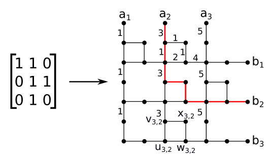
Figure 1: Illustration of the construction of Definition 1. The shortest path from $a_{2}$ to $b_{2}$ is highlighted in red. Most edge weights are omitted for clarity.

Proposition 1.

Let $M$ be a boolean $R\times C$ matrix and let $G_{M}$ be its grid embedding as defined in Definition 1. Then for any $1\leq i\leq R,1\leq j\leq C$ and $i<k\leq R$ the shortest path distance from $u_{i,j}$ to $b_{k}$ is exactly

$$(k-i)\cdot 2j+2R\cdot(C-j+1)$$

if $M_{k,j}=0$ and

$$(k-i)\cdot 2j+2R\cdot(C-j+1)-1$$

otherwise.

Proof.

Consider any shortest path from any $u_{i,j}$ to $b_{k}$. Such a path must always go either “right” or “down” (if $i=k$ the path must always go right). Essentially for every step to the left we pay at least $4R-1$ but can at most save $2R$: paying $2R$ going left and $2R$ going right, possibly saving $1$ with a shortcut, and saving $2$ for each vertical edge.

Now we will show the claim by induction on the sum $i+j$. Clearly, for $u_{R,C}$ to $b_{R}$ the distance is exactly $2R$. Now consider $u_{i,j}$ and assume $k>i$ as the case of $k=i$ is trivial. There are three cases to consider:

1. The path from $u_{i,j}$ goes through $w_{i,j}$ and then $u_{i,j+1}$. By the induction hypothesis this path has length at least

   $$2R+(k-i)\cdot 2(j+1)+2R\cdot(C-j)-1\geq 2R\cdot(C-j+1)+(k-i)\cdot 2j\ .$$

2. The path from $u_{i,j}$ goes through $v_{i+1,j}$ and then $x_{i+1,j}$, $w_{i+1,j}$, and $u_{i+1,j+1}$. This path is only available if $M_{i+1,j}=1$. If $k=i+1$, this distance is exactly

   $$2j-1+2R\cdot(C-j+1)\ .$$

   Otherwise, by the induction hypothesis, it is at least

   $$(k-i-1)\cdot 2(j+1)+2R\cdot(C-j)-1+2j+2R-1\geq(k-i)\cdot 2j+2R\cdot(C-j+1)$$

   for $k>i+1$

3. The path from $u_{i,j}$ goes through $v_{i+1,j}$ and then $u_{i+1,j}$. By the induction hypothesis, if $M_{k,j}=1$, the length of this path is

   $$(k-i-1)\cdot 2j+2R\cdot(C-j+1)-1+2j=(k-i)\cdot 2j+2R\cdot(C-j+1)-1$$

   and otherwise it is

   $$(k-i-1)\cdot 2j+2R\cdot(C-j+1)+2j\ .$$

It is easy to verify that taking the path down and right as illustrated in Figure 1 gives exactly the distances in the proposition, finishing the proof. ∎

The following useful property of our grid construction follows.

Corollary 1.

Let $M$ and $G_{M}$ be as in Proposition 1. Then for any $1\leq k\leq R,1\leq j\leq C$, the distance between $a_{j}$ and $b_{k}$ in $G_{M}$ is exactly determined by whether $M_{k,j}=1$. In this case the distance is $2R\cdot(C-j+1)+2jk-1$ and it is $2R\cdot(C-j+1)+2jk$ otherwise.

The following generalization for matrices with integer weights will be useful when reducing from APSP.

Definition 2.

Let $M$ be a $R\times C$ matrix with integer weights in $\{0,\ldots,X\}$. We will call the following construction the grid embedding of $M$.

Let $G_{M}$ be the grid embedding from Definition 1 for the all ones matrix of size $R\times C$ and multiply the weight of each edge by $X^{2}$. Furthermore, for each edge $(v_{i,j},x_{i,j})$ increase its weight by $M_{i,j}$.

Corollary 2.

Let $M$ be a $R\times C$ matrix with integer weights in $\{0,\ldots,X\}$ and let $G_{M}$ be its grid embedding. Then for any $1\leq k\leq R,1\leq j\leq C$, the distance between $a_{j}$ and $b_{k}$ in $G_{M}$ is exactly

$$X^{2}\cdot(2R\cdot(C-j+1)+2jk-1)+M_{k,j}$$

Corollary 2 follows from Corollary 1 by observing that any path from $a_{j}$ to $b_{k}$ not using the shortcut at intersection $(k,j)$ has distance at least $X^{2}\cdot(2R\cdot(C-j+1)+2jk)$ and since $M_{k,j}<X^{2}$ this distance is longer than using the shortcut. We remark that it would have been sufficient to multiply the weights by $(X+1)$ instead of $X^{2}$, but we do so to simplify a later argument.

3 Hardness of dynamic APSP in planar graphs

We will first show the following, simpler theorem and then generalize it to show trade-offs between query and update time.

Theorem 4.

No algorithm can solve the dynamic APSP problem in planar graphs on $N$ nodes with amortized update and query time $O(N^{\frac{1}{2}-\varepsilon})$ for any $\varepsilon>0$ unless Conjecture 1 is false. This holds even if only weight updates are allowed.

The main idea in proving Theorem 4 is to reduce from the APSP problem by first reducing to $(\min,+)$-Matrix-Mult and use the grid construction from Section 2 to represent the matrices to be multiplied. We then perform several shortest paths queries to simulate the multiplication process. Below, we first present a naïve and faulty approach explaining the main ideas of the reduction. We then show how to mend this approach giving the desired result.

Attempt 1.

Consider the following algorithm for solving an instance, $A\oplus B$ of the $(\min,+)$-Matrix-Mult problem, where $A$ and $B$ are $n\times n$ matrices. We may assume that $A$ and $B$ have integer weights in $\{0,\ldots,X\}$ for some $X=poly(n)$.

We let the initial graph of the problem be the grid embedding $G_{B}$ of $B$ according to Definition 2 along with a special vertex $t$. Also add the edges $(b_{k},t)$ for each $1\leq k\leq n$. Now we wish to construct $C=A\oplus B$ one row at a time. Such a row is a $(\min,+)$-product of a row in $A$ and the entire matrix $B$. Thus, for each row, $i$, of $A$ we have a phase as follows:

1. For each $1\leq k\leq n$ update the weight of the edge $(b_{k},t)$ to be $A_{i,k}$.

2. For each $1\leq j\leq n$ query the distance between $a_{j}$ and $t$.

The idea of each phase is that the distance between $a_{j}$ and $t$ should correspond to the value of $C_{i,j}=\min_{k}A_{i,k}+B_{k,j}$. Observe, that the distance from $a_{j}$ to $t$ using the edge $(b_{k},t)$ is exactly

$$X^{2}\cdot(2n\cdot(n-j+1)+2jk-1)+B_{k,j}+A_{i,k}$$

by Corollary 2. The dominant term in this expression increases with $k$ and thus no matter what $B_{k,j}$ and $A_{i,k}$ are (for $k>1$), the shortest path from $a_{j}$ to $t$ will simply pick $k=1$ minimizing the above expression. If we instead set the weight of each edge $(b_{k},t)$ to $X^{2}\cdot 2j(n-k)+A_{i,k}$ we get the distance of using this edge to be

$$X^{2}\cdot(2n\cdot(n-j+1)+2jk-1)+B_{k,j}+A_{i,k}+X^{2}\cdot 2j(n-k)=X^{2}\cdot(2n(n+1)-1)+B_{k,j}+A_{i,k}\ .$$

It follows that the shortest path from $a_{j}$ to $t$ is free to pick any $k$ while only affecting the $B_{k,j}+A_{i,k}$ term, which means that the shortest distance will be achieved by picking the $k$ minimizing this term, which would give us exactly $X^{2}\cdot(2n(n+1)-1)+C_{i,j}$. This approach therefore allows us to correctly calculate $C=A\oplus B$. However, the weight of the edge $(b_{k},t)$ now depends on which $a_{j}$ we are querying implying that we have to update this weight for each $a_{j}$ leading to a total of $O(n^{3})$ updates. By using this approach we are thus not able to make any statement about the time required for updates. We may try to assign edges and weights differently, but such approaches run into similar issues.

Observe that the graph created has $N=O(n^{2})$ nodes. Thus, if we were able to perform only $O(n^{2})$ total queries and updates the result of Theorem 4 would follow. $\Diamond$

In order to circumvent this dependence on $j$ when assigning weights to the edges $(b_{k},t)$ we instead replace $t$ by another grid whose purpose is to “normalize” the distance for each $a_{j}$. By doing this we can connect the grids with edges whose weight is independent of $j$. This step deviates significantly from the construction of [32] and is inspired by the grid tiling framework of Marx [50, 51].

Proof of Theorem 4.

We follow the same approach as in Attempt 1, but with a few changes. Define the initial graph $G$ as follows: Let $G_{B}$ be as before and let $G^{\prime}_{B}$ be the grid embedding of $B$ mirrored along the vertical axis with all shortcuts removed. Now for each $1\leq k\leq n$ add the edge $(b_{k},b^{\prime}_{k})$ and define $G$ to be this graph.

Now we perform a phase for each row $i$ of $A$ as follows:

1. For each $1\leq k\leq n$ set the weight of the edge $(b_{k},b^{\prime}_{k})$ to be $X^{2}\cdot(2(n+1)(n-k))+A_{i,k}$.

2. For each $j$ query the distance between $a_{j}$ and $a^{\prime}_{n-j+1}$.

An example of this construction for $n=3$ can be seen in Figure 2.

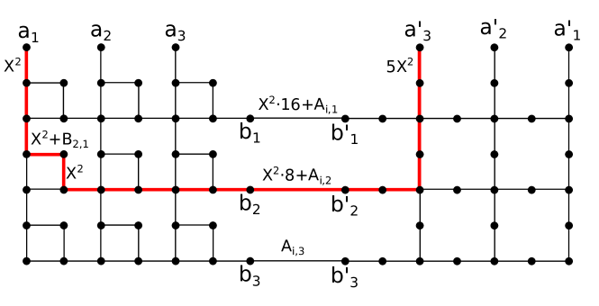
Figure 2: Example of a phase in the graph $G$ in the reduction of Theorem 4. The highlighted path illustrates a shortest path between $a_{1}$ and $a^{\prime}_{3}$ as an example of a query. Most edge weights have been omitted for clarity.

From the query between nodes $a_{j}$ and $a^{\prime}_{n-j+1}$ above during phase $i$ we can determine the entry $C_{i,j}$ of the output matrix. To see this, consider the distance from $a_{j}$ to $a^{\prime}_{n-j+1}$ at the time of query. This path has to go via some edge $(b_{k},b^{\prime}_{k})$. From Corollary 2 we know that this distance is exactly

$$d_{G}(a_{j},a^{\prime}_{n-j+1}) =d(a_{j},b_{k})+w(b_{k},b^{\prime}_{k})+d(b^{\prime}_{k},a^{\prime}_{n-j+1})$$

$$=X^{2}\cdot(2n\cdot(n-j+1)+2jk-1)+B_{k,j}+X^{2}\cdot(2(n+1)(n-k))+A_{i,k}$$

$$\qquad+X^{2}\cdot(2n\cdot j+2(n-j+1)k)$$

$$=X^{2}\cdot 2n(n+1)+X^{2}\cdot 2k(n+1)+X^{2}\cdot 2(n+1)(n-k)+B_{k,j}+A_{i,k}-X^{2}$$

$$=X^{2}\cdot 4n(n+1)-X^{2}+B_{k,j}+A_{i,k}\ .$$

The crucial property that our construction achieves is that the dominant term of this expression is independent of $k$. Thus, the shortest path will choose to go through the edge $(b_{k},b^{\prime}_{k})$ that minimizes $B_{k,j}+A_{i,k}$, implicitly giving us $C_{i,j}$. Subtracting $X^{2}\cdot(4n(n+1)-1)$ from the queried distance gives exactly the value of $C_{i,j}$ and the algorithm therefore correctly computes $C$.

Following the analysis from Attempt 1 we have that any algorithm with an amortized running time of $O(N^{\frac{1}{2}-\varepsilon})$ for both updates and queries contradicts Conjecture 1. ∎

3.1 Trade-offs

Theorem 4 above shows that no algorithm can perform both updates and queries in amortized time $O(N^{\frac{1}{2}-\varepsilon})$ unless Conjecture 1 is false. We will now show how to generalize these ideas to show Theorem 1.

Proof of Theorem 1.

The proof follows the same structure as the proof for Theorem 4, but instead of reducing from $(\min,+)$-Matrix-Mult on $n\times n$ matrices we reduce from an unbalanced version.

Let $A$ and $B$ be $n\times n^{\beta}$ and $n^{\beta}\times n^{\alpha}$ matrices respectively for some $0<\alpha,\beta\leq 1$. We define the initial graph $G$ from $B$ in the same manner as in Theorem 4. We then have a phase for each row $i$ of $A$ as follows:

1. For each $1\leq k\leq n^{\beta}$ set the weight of the edge $(b_{k},b^{\prime}_{k})$ to be $X^{2}\cdot(2(n^{\alpha}+1)(n^{\beta}-k))+A_{i,k}$.

2. For each $1\leq j\leq n^{\alpha}$ query the distance between $a_{j}$ and $a^{\prime}_{n^{\alpha}-j+1}$.

The entry $C_{i,j}$ is exactly the distance $d_{G}(a_{j},a^{\prime}_{n^{\alpha}-j+1})$ from the $i$th phase minus $X^{2}\cdot(4n^{\beta}(n^{\alpha}+1)-1)$. The correctness of the above reduction follows directly from the proof of Theorem 4 as well as Corollary 2.

Now observe that the graph $G$ from the above reduction has $N=\Theta(n^{\alpha+\beta})$ nodes and we perform a total of $O(n^{1+\alpha})$ queries and $O(n^{1+\beta})$ updates – that is, at most $O(n)$ updates per row and $O(n)$ queries per column. Any algorithm solving this problem must use total time $n^{1+\alpha+\beta-o(1)}$ time unless Conjecture 1 is false. It follows that either updates must take $n^{\alpha-o(1)}$ amortized time or queries must take $n^{\beta-o(1)}$ amortized time.

Assume now that an algorithm exists such that queries take $O(N^{\gamma})$ amortized time for any $0<\gamma<1$. We wish to show that this algorithm cannot perform updates in amortized time $O(N^{1-\gamma-\varepsilon})$ for any $\varepsilon>0$. Pick $\beta=\gamma+\varepsilon/2$ and set $\alpha=1-\beta$. We now use the above reduction to create a dynamic graph $G$ with $N=O(n^{\alpha+\beta})=O(n)$ nodes. Since queries do not take $n^{\beta-o(1)}$ time it follows from the above discussion that updates must take $n^{\alpha-o(1)}=n^{1-\gamma-\varepsilon/2-o(1)}$ time. Since this is polynomially greater than $O(N^{1-\gamma-\varepsilon})$ the claim follows. ∎

4 Hardness of dynamic maximum weight matching in bipartite planar graphs

In this section we will demonstrate the generality of our reduction framework by showing Theorem 3.

Proof of Theorem 3.

We start by showing how to reduce from $(\min,+)$-Matrix-Mult to minimum weight perfect matching, where the weight of such a matching corresponds to the shortest path distance between $a_{j}$ and $a^{\prime}_{n-j+1}$ similar to the proof of Theorem 1. We then describe how to use this reduction further to get a problem instance for maximum weight matching.

Let $A,B$ be an instance to the $(\min,+)$-Matrix-Mult problem of sizes $n\times n^{\beta}$ and $n^{\beta}\times n^{\alpha}$ respectively. Consider the grid embedding $G_{B}$ of $B$. We first replace each node of $G_{B}$ by two nodes connected by an edge of weight $0$. For $a_{j}$, $u_{i,j}$, $x_{i,j}$, and $v_{i,j}$ denote the corresponding nodes with superscript $d$ and $u$ (for “down” and “up”). For $b_{i}$ and $w_{i,j}$ denote the corresponding nodes with superscript $l$ and $r$ (for “left” and “right”). Now, for each original edge in $G_{B}$ we replace it as follows keeping its weight:

• $(u_{i,j},v_{i,j})\rightarrow(u_{i,j}^{u},v_{i,j}^{d})$

• $(u_{i,j},w_{i,j})\rightarrow(u_{i,j}^{d},w_{i,j}^{l})$

• $(u_{i,j},v_{i+1,j})\rightarrow(u_{i,j}^{d},v_{i+1,j}^{u})$

• $(u_{i,j},w_{i,j-1})\rightarrow(u_{i,j}^{u},w_{i,j-1}^{r})$

• $(v_{i,j},x_{i,j})\rightarrow(v_{i,j}^{d},x_{i,j}^{u})$

• $(x_{i,j},w_{i,j})\rightarrow(x_{i,j}^{d},w_{i,j}^{l})$

• $(a_{j},v_{0,j})\rightarrow(a_{j}^{d},v_{0,j}^{u})$

• $(w_{i,C},b_{i})\rightarrow(w_{i,C}^{r},b_{i}^{l})$

This construction is illustrated in Figure 3. We call this modified grid structure $\bar{G}_{B}$. Observe that there are no edges between “up” and “left” vertices or between “down” and “right”. It follows that the graph is bipartite and that these two sets of nodes make up the two partitions.

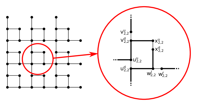
Figure 3: Grid construction for minimum weight perfect matching. Thick edges correspond to original edges and have the same weight as in $G_{B}$. Thin edges have weight $0$.

We now replace the grids $G_{B}$ and $G^{\prime}_{B}$ by $\bar{G}_{B}$ and $\bar{G}^{\prime}_{B}$ in the initial graph $G$ from the proof of Theorem 1. The edges $(b_{k},b^{\prime}_{k})$ are replaced by $(b^{r}_{k},b^{\prime l}_{k})$. We will use the following observation.

Proposition 2.

The graph resulting from joining two grids $\bar{G}_{B}$ in the way of Figure 2 has a unique perfect matching.

Proof.

It is easy to see that simply matching all weight $0$ edges gives a perfect matching. Thus we need to show that this is the only perfect matching. We will show the claim by a simple “peeling” argument.

Observe that $a_{1}^{u}$ only has one incident edge, so the edge $(a_{1}^{u},a_{1}^{d})$ must be in any perfect matching and we may “peel” away these two nodes. It now follows that $v_{1,1}^{u}$ only has one adjacent edge, so $(v_{1,1}^{u},v_{1,1}^{d})$ has to be in any perfect matching and we may peel away these nodes. Now $u_{1,1}^{u}$ only has one adjacent edge and so on for $v_{2,1}^{u}$, $u_{2,1}^{u}$, etc. This peels away the entire first column. Now each $x^{u}_{i,1}$ has only one adjacent edge matching this leaves each $w_{i,1}^{l}$ with only one adjacent edge. Peeling these nodes away leaves us with a smaller grid and we may start the argument over with $a_{2}$.

By doing this we see that the edge joining $b_{i}^{r}$ and $b_{i}^{\prime l}$ cannot be in a perfect matching as $(b_{i}^{r},b_{i}^{l})$ has to be. Thus we can repeat the same argument on the second grid. ∎

We now add two additional nodes $s$ and $t$ to the initial graph and perform a phase for each row $i$ of $A$ as follows:

1. For each $1\leq k\leq n^{\beta}$ set the weight of the edge $(b^{r}_{k},b^{\prime l}_{k})$ to be $X^{2}\cdot(2(n^{\alpha}+1)(n^{\beta}-k))+A_{i,k}$.

2. For each $1\leq j\leq n^{\alpha}$ do the following three steps: 1) add the edges $(s,a^{u}_{j})$ and $(t,a^{\prime u}_{n^{\alpha}-j+1})$, 2) query the minimum weight perfect matching, 3) delete the two edges.

Since the edges $(s,a^{u}_{j})$ and $(t,a^{\prime u}_{n^{\alpha}-j+1})$ have to be in any perfect matching this leaves $a^{d}_{j}$ and $a^{\prime d}_{n^{\alpha}-j+1}$ unmatched. Any perfect matching now has to “connect” these two nodes by a path of original (weight $>0$) edges. The weight of a perfect matching in $G$ then corresponds to the length of a shortest path from $a_{j}$ to $a^{\prime}_{n^{\alpha}-j+1}$ in the graph from the proof of Theorem 1. It follows that we get the same trade-offs for minimum weight perfect matching as for APSP with the exception that the trade-off only holds when $q(N)\geq u(N)$ since we perform $O(1)$ updates for each query.

To show the same result for maximum weight matching we may simply perform the following two changes: 1) pick a sufficiently large integer $y$ and set the weight of each edge to $y$ minus its weight in the above reduction, and 2) when adding the edges $(s,a^{u}_{j})$ and $(t,a^{\prime u}_{n^{\alpha}-j+1})$ assign them weight $y^{2}$ such that any maximum weight matching has to include these two edges and will have weight

$$y^{2}+\frac{N-4}{2}\cdot y-d_{G*}(a_{j},a^{\prime}_{n^{\alpha}-j+1})\ ,$$

where $G*$ denotes the corresponding graph in the proof of Theorem 1. ∎

5 Unweighted

The proofs of the previous sections rely heavily on the weighted grid from Section 2. We may generalize the ideas to the unweighted case by instead using the grid of Definition 1 and subdividing the edges giving us somewhat weaker bounds. This gives us Theorem 2.

The problem we reduce from is the online matrix-vector problem from [38]. We may define this problem as follows: Let $M$ be a $n\times n$ matrix and let $v^{1},\ldots,v^{n}$ be $n$ boolean vectors arriving in an online fashion. The task is to pre-process $M$ such that we can output the product $Mv^{i}$ for each $i$ before seeing $v^{i+1}$. It was conjectured in [38] that this problem takes $n^{3-o(1)}$ time, while the best known upper bound is $n^{3}/2^{\Omega(\sqrt{\log{n}})}$ [48]. Known reductions from [64] show that this conjecture implies a $n^{1+\alpha+\beta-o(1)}$ bound for the following problem: Let $\alpha,\beta>0$ be fixed constants and let $M$ be a boolean $n^{\beta}\times n^{\alpha}$ matrix (see [38] for the details). After preprocessing $M$, $n$ boolean vector pairs $(u^{1},v^{1}),\ldots,(u^{n},v^{n})\in\{0,1\}^{n^{\beta}}\times\{0,1\}^{n^{\alpha}}$ arrive one at a time and the task is to compute $(u^{i})^{T}Mv^{i}$ before being presented with the $i+1$th vector pair for every $i$. We will use this problem called the OuMv problem to reduce to unit weight dynamic APSP in planar graphs below.

Proof of Theorem 2.

Consider the reduction from Theorem 1 using a $n^{\beta}\times n^{\alpha}$ grid. We will use a similar approach to solve the OuMv problem below.

Let $M$ be the $n^{\beta}\times n^{\alpha}$ matrix of the OuMv problem and create $G_{M}$ according to Definition 1 (note that this grid embedding is different from the one used in the proof of Theorem 1). We also add $G^{\prime}_{M}$ similarly to the proof of Theorem 1. We then subdivide each edge into a path of the same length. We also add to $G$ a path of length $2(n^{\alpha}+1)(n^{\beta}-k)$ connecting $b_{k}$ and $b^{\prime}_{k}$ for each $1\leq k\leq n^{\beta}$. We then disconnect $b_{k}$ and $b^{\prime}_{k}$ from this path.

We perform a phase as follows for each vector pair $(u^{i},v^{i})$:

1. For each $k$ such that $u^{i}_{k}=1$ connect $b_{k}$ and $b^{\prime}_{k}$ to their respective path.

2. For each $j$ such that $v^{i}_{j}=1$ query the distance from $a_{j}$ to $a^{\prime}_{n^{\alpha}-j+1}$.

3. Remove all the edges added in step 1.

If the answer to any of the queries during the $i$th phase is $4n(n+1)-1$ the answer to the $i$th product is $1$ and otherwise the answer is $0$. This follows from Corollary 1 in the same way as Theorem 1.

By subdividing the edges we get a graph with $N=O(n^{2\beta+\alpha}+n^{2\alpha+\beta})$ nodes. We perform $O(n^{1+\alpha})$ queries and $O(n^{1+\beta})$ updates. It follows from the OMv conjecture that the entire process must take $n^{1+\beta+\alpha-o(1)}$ time, thus either updates take $n^{\alpha-o(1)}$ time or queries take $n^{\beta-o(1)}$ time.

We will assume that $q(N)\geq u(N)$ and note that the other case follows symmetrically. Assume that some algorithm can perform queries in $N^{\gamma}$ for some $\frac{1}{3}\leq\gamma<\frac{1}{2}$. We wish to show that this algorithm cannot perform updates in time $N^{1-2\gamma-\varepsilon}$ for any $\varepsilon>0$. To do this, pick $\beta=\gamma+\varepsilon/3$ and $\alpha=1-2\beta$. Note that $\beta\geq\alpha$ (corresponding to $q(N)\geq u(N)$). Thus the graph has $N=O(n^{2\beta+\alpha})=O(n)$ nodes. It now follows by the above discussion that the algorithm cannot perform updates faster than $n^{\alpha-o(1)}=N^{1-2\gamma-2\varepsilon/3+o(1)}$ which proves the claim.

Finally, observe that by using an $n\times n$ matrix in the above reduction (i.e. $\alpha=\beta=1$) we see that at least one of updates and queries have to take $n^{\frac{1}{3}-o(1)}$ amortized time (similar to Theorem 4). ∎

To see that we may do the above reduction while keeping the dynamic graph $G$ as a grid graph, observe that we may multiply the weight of each edge before subdividing by a large enough constant and then “zig-zag” the subdivided edges in order to fit the grid structure. This is illustrated in Figure 4.

Figure 4: Illustration of the grid created in the proof of Theorem 2. Dashed edges correspond to possible shortcuts. Note that the lengths of the edges are not to scale!

6 Dynamic $s,t$-shortest path and related problems

In Section 3 we showed a lower bound for the trade-off between query and update time for dynamic APSP in grid graphs conditioned on Conjecture 1. Here we will argue that the proof of Theorem 1 can be extended to show similar lower bounds for dynamic problems, where the algorithm only needs to maintain a single value such as $s,t$-shortest path, girth, and diameter. We also note that the above techniques for proving bounds in unweighted graphs also apply to the theorem below.

Theorem 5.

No algorithm can solve the $s,t$-shortest path, girth (directed), or diameter problems in planar graphs on $N$ nodes with amortized update time $u(N)$ and query time $q(N)$ such that $\max(q(N),u(N))=O(N^{\frac{1}{2}-\varepsilon})$ for any $\varepsilon>0$ unless Conjecture 1 is false. Furthermore, if $q(N)\geq u(N)$ the algorithm cannot have $q(N)\cdot u(N)=O(N^{1-\varepsilon})$. This holds even if the planar embedding of $G$ never changes.

Proof.

We note that the proof follows the exact same structure as the proof of Theorem 1 and only mention the changes needed to be made.

For $s,t$-shortest path and diameter we add two additional nodes $s,t$ to the initial graph $G$ and when performing a query of the distance between $a_{j}$ and $a^{\prime}_{n^{\alpha}-j+1}$ we instead insert edges $(s,a_{j})$ and $(t,a^{\prime}_{n^{\alpha}-j+1})$ of sufficiently high weight so that this is the longest distance in the graph and query the $s,t$ distance.

For girth we direct all horizontal edges of $G$ to the right, all vertical edges of the left grid down and all vertical edges of the right grid up. When doing a query we add the directed edge $(a^{\prime}_{n^{\alpha}-j+1},a_{j})$ with weight $1$, and the length of the shortest cycle then corresponds to the shortest path from $a_{j}$ to $a^{\prime}_{n^{\alpha}-j+1}$ plus $1$. ∎

In the above reductions, the condition $q(N)\geq u(N)$ comes from the fact that we perform $O(1)$ updates for every query we make and the argument from Theorem 1 thus breaks down if we try to argue for slower updates than queries. This makes sense from an upper bound perspective: clearly, any algorithm with $q(N)\leq u(N)$ could simply perform a query for every update, store the answer, and then provide queries in $O(1)$ time.

7 Weight updates

We mentioned in the previous sections that the results hold even if we only allow weight updates instead of edge insertions/deletions. In [6] they considered this model in which the algorithm is supplied with an initial graph $G$ and a promise that for any updated graph $G^{\prime}$ we have $d_{G}(u,v)\leq d_{G^{\prime}}(u,v)\leq M\cdot d_{G}(u,v)$ for all $u,v\in G$ and some parameter $M>1$. The only operations allowed are weight updates and queries. We note that all the above results for weighted graphs also hold in this model.

As a proof sketch, consider the result of Theorem 1: The only edges whose weight changes are the “in-between” edges $(b_{k},b^{\prime}_{k})$ whose weights are always between $X^{2}\cdot(2(n^{\alpha}+1)(n^{\beta}-k)$ and $X^{2}\cdot(2(n^{\alpha}+1)(n^{\beta}-k))+X$. Similarly, for $s,t$-shortest path and diameter: Assume that the edge $(s,a_{j})$ has weight $y$ when added in the reduction of Theorem 5. We may instead initialize the graph $G$ with an edge $(s,a_{j})$ of weight $y$ for each $1\leq j\leq n^{\alpha}$, increase each edge to have weight $M\cdot y$ and then instead of adding the edge $(s,a_{j})$ we decrease its weight back to $y$. We do the same for $t$ and the nodes $a^{\prime}_{j}$. By picking $y$ sufficiently large we may ensure that an edge of weight $M\cdot y$ cannot be on the shortest path from $s$ to $t$. Furthermore these changes can still be done while maintaining the graphs as grids.

8 Worst-case bounds for partially dynamic problems

Our reductions above work in the fully dynamic setting, where edge insertions and deletions (or weight increments and decrements) are allowed. We now show that, using standard techniques, we can turn these amortized bounds into worst-case bounds for the same problem in the incremental and decremental (only insertions/increments or deletions/decrements allowed). We will show the result for dynamic APSP and note that the method is the same for the other problems.

Corollary 3.

No algorithm can solve the incremental or decremental APSP problem for planar graphs on $N$ nodes with worst-case query time $q(N)$ and update time $u(N)$ such that $q(N)\cdot u(N)=O(N^{1-\varepsilon})$ for any $\varepsilon>0$ unless Conjecture 1 is false.

Proof.

We present the argument for the problem when we are given an initial graph $G$ and are only allowed to increase weights on edges. The proof uses the same rollback technique employed before in several papers (see e.g. [3]).

First we create the same initial graph, $G$, as in the proof of Theorem 1. We set the initial weight of the edges $(b_{k},b^{\prime}_{k})$ to be $X^{2}\cdot(2(n^{\alpha}+1)(n^{\beta}-k))$. During the phase of each row $i$ of $A$ we keep track of all memory changes made by the incremental data structure while increasing each edge to have weight $X^{2}\cdot(2(n^{\alpha}+1)(n^{\beta}-k))+A_{i,k}$. We then perform each distance query and instead of deleting the incremented edges, we “roll back” the data structure using the memory changes we kept track of, thus restoring $G$ to its initial state. By doing this we solve the $(\min,+)$-Matrix-Mult problem in the exact same way as in Theorem 1. However, we cannot ensure any requirement on the amortized running time, as the rollback operations may essentially “restore all credit” to the data structure in the sense of amortized analysis. Thus, the time bounds only apply to worst-case running times. ∎

Acknowledgements

The authors would like to acknowledge Shay Mozes, Oren Weimann and Virginia Vassilevska Williams for helpful comments and discussions.

References

- [1] Amir Abboud, Fabrizio Grandoni, and Virginia Vassilevska Williams. Subcubic equivalences between graph centrality problems, APSP and diameter. In Proc. 26th ACM/SIAM Symposium on Discrete Algorithms (SODA), pages 1681–1697, 2015.
- [2] Amir Abboud and Kevin Lewi. Exact weight subgraphs and the k-sum conjecture. In Proc. 40th International Colloquium on Automata, Languages and Programming (ICALP), pages 1–12, 2013.
- [3] Amir Abboud and Virginia Vassilevska Williams. Popular conjectures imply strong lower bounds for dynamic problems. In Proc. 55th IEEE Symposium on Foundations of Computer Science (FOCS), pages 434–443, 2014.
- [4] Amir Abboud, Virginia Vassilevska Williams, and Joshua R. Wang. Approximation and fixed parameter subquadratic algorithms for radius and diameter in sparse graphs. In Proceedings of the Twenty-Seventh Annual ACM-SIAM Symposium on Discrete Algorithms, SODA 2016, Arlington, VA, USA, January 10-12, 2016, pages 377–391, 2016.
- [5] Amir Abboud, Virginia Vassilevska Williams, and Huacheng Yu. Matching triangles and basing hardness on an extremely popular conjecture. In Proc. 47th ACM Symposium on Theory of Computing (STOC), pages 41–50, 2015.
- [6] Ittai Abraham, Shiri Chechik, Daniel Delling, Andrew V. Goldberg, and Renato F. Werneck. On dynamic approximate shortest paths for planar graphs with worst-case costs. In Proc. 27th ACM/SIAM Symposium on Discrete Algorithms (SODA), pages 740–753, 2016.
- [7] Ittai Abraham, Shiri Chechik, and Cyril Gavoille. Fully dynamic approximate distance oracles for planar graphs via forbidden-set distance labels. In Proc. 44th ACM Symposium on Theory of Computing (STOC), pages 1199–1218, 2012.
- [8] Stephen Alstrup, Søren Dahlgaard, Mathias Bæk Tejs Knudsen, and Ely Porat. Sublinear distance labeling for sparse graphs. CoRR, abs/1507.02618, 2015.
- [9] Stephen Alstrup, Cyril Gavoille, Esben Bistrup Halvorsen, and Holger Petersen. Simpler, faster and shorter labels for distances in graphs. In Proc. 27th ACM/SIAM Symposium on Discrete Algorithms (SODA), pages 338–350, 2016.
- [10] Abhash Anand, Surender Baswana, Manoj Gupta, and Sandeep Sen. Maintaining approximate maximum weighted matching in fully dynamic graphs. In Conference on the Foundations of Software Technology and Theoretical Computer Science (FSTTCS), pages 257–266, 2012.
- [11] Rinat Ben Avraham, Haim Kaplan, and Micha Sharir. A faster algorithm for the discrete fréchet distance under translation. arXiv preprint arXiv:1501.03724, 2015.
- [12] Surender Baswana, Manoj Gupta, and Sandeep Sen. Fully dynamic maximal matching in o (log n) update time. In Foundations of Computer Science (FOCS), 2011 IEEE 52nd Annual Symposium on, pages 383–392. IEEE, 2011.
- [13] Reinhard Bauer. Dynamic speed-up techniques for dijkstra?s algorithm. Master’s thesis, Institut für Theoretische Informatik-Universität Karlsruhe (TH), page 41, 2006.
- [14] Aaron Bernstein and Cliff Stein. Fully dynamic matching in bipartite graphs. In Automata, Languages, and Programming, pages 167–179. Springer, 2015.
- [15] Aaron Bernstein and Cliff Stein. Faster fully dynamic matchings with small approximation ratios. In Proceedings of the Twenty-Seventh Annual ACM-SIAM Symposium on Discrete Algorithms, pages 692–711. SIAM, 2016.
- [16] Sayan Bhattacharya, Monika Henzinger, and Giuseppe F Italiano. Deterministic fully dynamic data structures for vertex cover and matching. In Proceedings of the Twenty-Sixth Annual ACM-SIAM Symposium on Discrete Algorithms, pages 785–804. SIAM, 2015.
- [17] Glencora Borradaile, Philip N. Klein, Shay Mozes, Yahav Nussbaum, and Christian Wulff-Nilsen. Multiple-source multiple-sink maximum flow in directed planar graphs in near-linear time. In Proc. 52nd IEEE Symposium on Foundations of Computer Science (FOCS), pages 170–179, 2011.
- [18] Raphaël Clifford, Allan Grønlund, and Kasper Green Larsen. New unconditional hardness results for dynamic and online problems. In Proc. 56th IEEE Symposium on Foundations of Computer Science (FOCS), pages 1089–1107, 2015.
- [19] Søren Dahlgaard. On the hardness of partially dynamic graph problems and connections to diameter. arXiv preprint arXiv:1602.06705, 2016. To appear at ICALP’16.
- [20] Daniel Delling, Andrew V Goldberg, Thomas Pajor, and Renato F Werneck. Customizable route planning. In Experimental algorithms, pages 376–387. Springer, 2011.
- [21] Daniel Delling, Peter Sanders, Dominik Schultes, and Dorothea Wagner. Engineering route planning algorithms. In Algorithmics of large and complex networks, pages 117–139. Springer, 2009.
- [22] Daniel Delling and Dorothea Wagner. Landmark-based routing in dynamic graphs. In Experimental algorithms, pages 52–65. Springer, 2007.
- [23] Krzysztof Diks and Piotr Sankowski. Dynamic plane transitive closure. In Algorithms–ESA 2007, pages 594–604. Springer, 2007.
- [24] Hristo N Djidjev, Grammati E Pantziou, and Christos D Zaroliagis. Computing shortest paths and distances in planar graphs. In Automata, Languages and Programming, pages 327–338. Springer, 1991.
- [25] Dorit Dor, Shay Halperin, and Uri Zwick. All-pairs almost shortest paths. SIAM Journal on Computing, 29(5):1740–1759, 2000.
- [26] Ran Duan and Seth Pettie. Linear-time approximation for maximum weight matching. Journal of the ACM (JACM), 61(1):1, 2014.
- [27] David Eppstein. Dynamic connectivity in digital images. Information Processing Letters, 62(3):121–126, 1997.
- [28] Jittat Fakcharoenphol and Satish Rao. Planar graphs, negative weight edges, shortest paths, and near linear time. Journal of Computer and System Sciences, 72(5):868–889, 2006. See also FOCS’01.
- [29] Greg N Frederickson. Data structures for on-line updating of minimum spanning trees, with applications. SIAM Journal on Computing, 14(4):781–798, 1985.
- [30] Zvi Galil and Giuseppe F Italiano. Maintaining biconnected components of dynamic planar graphs. Springer, 1991.
- [31] Zvi Galil, Giuseppe F Italiano, and Neil Sarnak. Fully dynamic planarity testing. In Proceedings of the twenty-fourth annual ACM symposium on Theory of computing, pages 495–506. ACM, 1992.
- [32] Cyril Gavoille, David Peleg, Stéphane Pérennes, and Ran Raz. Distance labeling in graphs. Journal of Algorithms, 53(1):85–112, 2004. See also SODA’01.
- [33] Pawel Gawrychowski and Adam Karczmarz. Improved bounds for shortest paths in dense distance graphs. CoRR, abs/1602.07013, 2016.
- [34] Robert Geisberger, Peter Sanders, Dominik Schultes, and Christian Vetter. Exact routing in large road networks using contraction hierarchies. Transportation Science, 46(3):388–404, 2012.
- [35] Madhu Gupta and Rongkun Peng. Fully dynamic (1+ e)-approximate matchings. In Foundations of Computer Science (FOCS), 2013 IEEE 54th Annual Symposium on, pages 548–557. IEEE, 2013.
- [36] Rohit Gurjar, Arpita Korwar, Jochen Messner, Simon Straub, and Thomas Thierauf. Planarizing gadgets for perfect matching do not exist. In Mathematical Foundations of Computer Science 2012, pages 478–490. Springer, 2012.
- [37] Meng He, Ganggui Tang, and Norbert Zeh. Orienting dynamic graphs, with applications to maximal matchings and adjacency queries. In Algorithms and Computation, pages 128–140. Springer, 2014.
- [38] Monika Henzinger, Sebastian Krinninger, Danupon Nanongkai, and Thatchaphol Saranurak. Unifying and strengthening hardness for dynamic problems via the online matrix-vector multiplication conjecture. In Proc. 47th ACM Symposium on Theory of Computing (STOC), pages 21–30, 2015.
- [39] Monika R Henzinger, Philip Klein, Satish Rao, and Sairam Subramanian. Faster shortest-path algorithms for planar graphs. journal of computer and system sciences, 55(1):3–23, 1997.
- [40] Giuseppe F Italiano, Yahav Nussbaum, Piotr Sankowski, and Christian Wulff-Nilsen. Improved algorithms for min cut and max flow in undirected planar graphs. In Proceedings of the forty-third annual ACM symposium on Theory of computing, pages 313–322. ACM, 2011.
- [41] Haim Kaplan, Shay Mozes, Yahav Nussbaum, and Micha Sharir. Submatrix maximum queries in monge matrices and monge partial matrices, and their applications. In Proceedings of the twenty-third annual ACM-SIAM symposium on Discrete Algorithms, pages 338–355. SIAM, 2012.
- [42] Philip Klein and Shay Mozes. Optimization algorithms for planar graphs, 2014. Book draft available at http://planarity.org.
- [43] Philip N Klein. Multiple-source shortest paths in planar graphs. In SODA, volume 5, pages 146–155, 2005.
- [44] Philip N Klein and Sairam Subramanian. A fully dynamic approximation scheme for shortest paths in planar graphs. Algorithmica, 22(3):235–249, 1998.
- [45] Tsvi Kopelowitz, Robert Krauthgamer, Ely Porat, and Shay Solomon. Orienting fully dynamic graphs with worst-case time bounds. In Automata, Languages, and Programming, pages 532–543. Springer, 2014.
- [46] Tsvi Kopelowitz, Seth Pettie, and Ely Porat. Higher lower bounds from the 3sum conjecture. In Proc. 27th ACM/SIAM Symposium on Discrete Algorithms (SODA), pages 1272–1287, 2016.
- [47] Jakub Łącki, Yahav Nussbaum, Piotr Sankowski, and Christian Wulff-Nilsen. Single source–all sinks max flows in planar digraphs. In Foundations of Computer Science (focs), 2012 Ieee 53rd Annual Symposium on, pages 599–608. IEEE, 2012.
- [48] Kasper Green Larsen and Ryan Williams. Faster online matrix-vector multiplication. arXiv preprint arXiv:1605.01695, 2016.
- [49] François Le Gall. Powers of tensors and fast matrix multiplication. In Proceedings of the 39th international symposium on symbolic and algebraic computation, pages 296–303. ACM, 2014.
- [50] Dániel Marx. On the optimality of planar and geometric approximation schemes. In Foundations of Computer Science, 2007. FOCS’07. 48th Annual IEEE Symposium on, pages 338–348. IEEE, 2007.
- [51] Dániel Marx. The square root phenomenon in planar graphs. In ICALP (2), page 28, 2013.
- [52] Ofer Neiman and Shay Solomon. Simple deterministic algorithms for fully dynamic maximal matching. ACM Transactions on Algorithms (TALG), 12(1):7, 2015. See also STOC’13.
- [53] Krzysztof Onak and Ronitt Rubinfeld. Maintaining a large matching and a small vertex cover. In Proceedings of the forty-second ACM symposium on Theory of computing, pages 457–464. ACM, 2010.
- [54] Mihai Patrascu. Towards polynomial lower bounds for dynamic problems. In Proc. 42nd ACM Symposium on Theory of Computing (STOC), pages 603–610, 2010.
- [55] David Peleg and Shay Solomon. Dynamic (1+ )-approximate matchings: a density-sensitive approach. In Proceedings of the Twenty-Seventh Annual ACM-SIAM Symposium on Discrete Algorithms, pages 712–729. SIAM, 2016.
- [56] Liam Roditty and Virginia Vassilevska Williams. Fast approximation algorithms for the diameter and radius of sparse graphs. In Proc. 45th ACM Symposium on Theory of Computing (STOC), pages 515–524, 2013.
- [57] Liam Roditty and Uri Zwick. On dynamic shortest paths problems. Algorithmica, 61(2):389–401, 2011. See also ESA’04.
- [58] Barna Saha. Language edit distance and maximum likelihood parsing of stochastic grammars: Faster algorithms and connection to fundamental graph problems. In Foundations of Computer Science (FOCS), 2015 IEEE 56th Annual Symposium on, pages 118–135. IEEE, 2015.
- [59] Piotr Sankowski. Faster dynamic matchings and vertex connectivity. In Proc. 18th ACM/SIAM Symposium on Discrete Algorithms (SODA), pages 118–126, 2007.
- [60] Dominik Schultes and Peter Sanders. Dynamic highway-node routing. In Experimental Algorithms, pages 66–79. Springer, 2007.
- [61] Sairam Subramanian. A fully dynamic data structure for reachability in planar digraphs. In Algorithms-ESA’93, pages 372–383. Springer, 1993.
- [62] Oren Weimann and Raphael Yuster. Approximating the diameter of planar graphs in near linear time. ACM Transactions on Algorithms, 12(1):12, 2016. See also ICALP’13.
- [63] Virginia Vassilevska Williams. Multiplying matrices faster than coppersmith-winograd. In Proceedings of the forty-fourth annual ACM symposium on Theory of computing, pages 887–898. ACM, 2012.
- [64] Virginia Vassilevska Williams and Ryan Williams. Subcubic equivalences between path, matrix and triangle problems. In Foundations of Computer Science (FOCS), 2010 51st Annual IEEE Symposium on, pages 645–654. IEEE, 2010.