Summary of the 2015 LHCb workshop on multi-body decays of $D$ and $B$ mesons

Abstract

This document contains a summary of the LHCb workshop on multi-body decays of $D$ and $B$ mesons, held at CBPF, Rio de Janeiro, in July 2015. The workshop was focused on issues related to amplitude analysis of three- and four-body hadronic decays. In addition to selected LHCb results, contributions from guest theorists are included.

I Introduction

Jonas Rademacker^a and Alberto C. dos Reis^b

^aH. H. Wills Physics Laboratory, University of Bristol,
Bristol, United Kingdom ^bCentro Brasileiro de Pesquisas Físicas – CBPF
Rio de Janeiro, Brazil

The study of multi-body hadronic decays of $D$ and $B$ mesons is very important in many respects. The very large samples available after LHCb allow for precision measurements, opening interesting possibilities in fields such as CP violation, mixing, heavy and light meson spectroscopy.

The analysis of these data and the interpretation of the results, however, involve rather intricate aspects, since multi-body hadronic decays involve a complex interplay between weak and low-energy strong interactions. Traditional approaches techniques and tools are no longer satisfactory. Improved models are required for extracting the most information from the new data. With this motivation, a LHCb workshop on amplitude analysis of multi-body took place in July, 2015, with the participation of invited theorists.

To trigger the discussions, a number of questions were proposed:

• Rescattering is an important ingredient which is not included in the usual decay models. How do one describes it in $D$ and $B$ decays? What role could combined analyses in multiple decay channels play?

• Quarks and hadrons — To what extent can one think of penguin diagrams when dealing with exclusive channels? When is it not useful anymore to think in terms of quark-level diagrams? What should one do instead? Ideally, one should explore the connection between the quark and hadron degrees of freedom to built sound parameterisations of nonresonant amplitudes. This is obviously a rather intricate problem. Is there any alternative approach?

• Symmetries — To what extend is it useful to use approximate symmetries like isospin, U-spin, V-spin, SU(3)-flavour? How can we quantify the effects of the breaking of those symmetries? Fundamental principles, such as unitarity, analyticity and CPT conservation, are widely used in $2\to 2$ processes to constrain and to relate the scattering amplitudes. How could one implement such constraints in the context of a hadronic weak decay of a heavy meson?

• Translatable results — What are the limitations and opportunities for using $2\to 2$ scattering results for describing $1\to 3$ decays? What about $1\to 4$ decays? What are the limitations of invoking Watson theorem in this context? Can the (model-independent) results for $\pi\pi$ and other line shapes obtained by COMPASS be directly applied to modeling the (weak) multi-body decays of $D$ and $B$ mesons? To what degree are mass/width results (such as those from Breit Wigner-based analyses, but also others) translatable between different experiments?

• The statistical precision in charm Dalitz analyses is unprecedented. What to do with these extremely clean, huge data samples (some with tens of millions of events), if one does not have models that are anywhere near precise enough to describe them?

• Threshold data provide a way of measuring phases across Dalitz plots in a model-independent fashion. As a matter of fact, this was used in model-independent analyses. Should one uses this unique information instead to build better models? Why is the CP-odd content of $D^{0}\to\pi\pi\pi^{0}$  100%? What does the CP-odd content of  75% in other investigated $D^{0}$ decay modes, such as $D^{0}\to 4\pi$, $D^{0}\to KK\pi^{0}$, tell us? Can this be used to test models?

• New resonances — How can one determine whether an observed structure corresponds to a new state or to some kind of threshold effect? Does an Argand plot with the phase motion (and its direction) tell us anything about that?

This document contains a summary of the discussions held at the LHCb workshop, with individual contributions from the guest theorists addressing the above and related questions. A non-exhaustive set of LHCb results on amplitude analysis is also presented.

II LHCb - summary of $B\to Dhh^{\prime}$ analyses

Mark Whitehead, for the LHCb collaboration

Department of Physics, University of Warwick,
Coventry, United Kingdom

II.1 Introduction

Results from the following analyses were presented at the workshop $B^{0}_{s}\to\overline{D}{}^{0}K^{-}\pi^{+}$ Aaij et al. (2014a), $B^{+}\to D^{-}K^{+}\pi^{-}$ Aaij et al. (2015a), $B^{0}\to\overline{D}{}^{0}\pi^{+}\pi^{-}$ Aaij et al. (2015b), $B^{0}\to\overline{D}{}^{0}K^{+}\pi^{-}$ Aaij et al. (2015c), $B^{0}\to DK^{+}\pi^{-}$ and $\Lambda^{0}_{b}\to D^{0}p\pi^{-}$. Of these, the first four are published results whilst the last two analyses are currently active. These decays modes can be used to study spectroscopy in the $DK$, $D\pi$, $Dp$, $K\pi$, $\pi\pi$ and $p\pi$ systems, and so have a wide and important role in the understanding of such resonant states. Additionally, amplitude analyses of some $B\to Dhh^{\prime}$ channels can be used to measure $CP$ violation. The decay $B^{0}\to DK^{+}\pi^{-}$, with $D\to K^{+}K^{-}\,,\pi^{+}\pi^{-}$, can be used to measure the CKM angle $\gamma$ Gershon (2009); Gershon and Williams (2009) and the CKM angle $\beta$ can be measured using $B^{0}\to\overline{D}{}^{0}\pi^{+}\pi^{-}$ decays Latham and Gershon (2009); Charles et al. (1998).

II.2 Summary of results

The Dalitz plot analysis of $B^{0}_{s}\to\overline{D}{}^{0}K^{-}\pi^{+}$ decays found that a resonance previously seen in inclusive $DK$ events, the so called $D^{*}_{sJ}(2860)^{+}$, is actually comprised of two overlapping states of different spin. Figure 1 shows the cosine of the helicity angle of the $DK$ system in the region $2770<m(DK)<2910$ MeV/$c^{2}$, with fits including spin 1, spin 3 and both spin 1 and spin 3 contributions overlaid. The reported masses and widths of these states are

$$m(D^{*}_{s1}(2860)^{+}) = 2859\pm 12\pm 6\pm 23\,{\rm MeV/c^{2}},$$

$$\Gamma(D^{*}_{s1}(2860)^{+}) = 159\pm 23\pm 27\pm 72\,{\rm MeV/c^{2}},$$

$$m(D^{*}_{s3}(2860)^{+}) = 2860.5\pm 2.6\pm 2.5\pm 6.0\,{\rm MeV/c^{2}},$$

$$\Gamma(D^{*}_{s3}(2860)^{+}) = 53\pm 7\pm 4\pm 6\,{\rm MeV/c^{2}},$$

where the uncertainties are statistical, experimental systematic and model systematic, respectively.

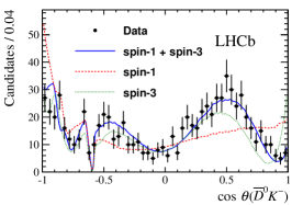
Figure 1: Projections of data and fit models on to the cosine of the helicity angle of the $DK$ system for $B^{0}_{s}\to\overline{D}{}^{0}K^{-}\pi^{+}$ decays in the mass window $2770<m(DK)<2910$ MeV/$c^{2}$. The data are black points and the fit models are described in the legend.

Analyses of $B^{+}\to D^{-}K^{+}\pi^{-}$, $B^{0}\to\overline{D}{}^{0}\pi^{+}\pi^{-}$ and $B^{0}\to\overline{D}{}^{0}K^{+}\pi^{-}$ decays showed the equivalent results for $D\pi$ resonances. The previously seen $D^{*}_{J}(2760)$ was found to be spin 1 using $B^{+}\to D^{-}K^{+}\pi^{-}$ decays while a spin 3 state was observed in the $B^{0}\to\overline{D}{}^{0}\pi^{+}\pi^{-}$ final state. Note that the $B^{+}$ analysis sees neutral charm mesons while the $B^{0}$ final state is sensitive to charged charm states. For $B^{0}\to\overline{D}{}^{0}K^{+}\pi^{-}$ decays no evidence for a $D^{*}_{J}(2760)$ state was found. Figure 2 shows the distribution of $m(D\pi)$ for $B^{+}\to D^{-}K^{+}\pi^{-}$, $B^{0}\to\overline{D}{}^{0}\pi^{+}\pi^{-}$ and $B^{0}\to\overline{D}{}^{0}K^{+}\pi^{-}$ final states together with the amplitude fit projections. The masses and widths of the $D^{*}_{J}(2760)$ states are

$$m(D^{*}_{1}(2760)^{0}) = 2781\pm 18\pm 11\pm 6\,{\rm MeV/c^{2}},$$

$$\Gamma(D^{*}_{1}(2760)^{0}) = 177\pm 32\pm 20\pm 7\,{\rm MeV/c^{2}},$$

$$m(D^{*}_{3}(2760)^{+}) = 2798\pm 7\pm 1\pm 7\,{\rm MeV/c^{2}},$$

$$\Gamma(D^{*}_{3}(2760)^{+}) = 105\pm 18\pm 6\pm 23\,{\rm MeV/c^{2}},$$

where the uncertainties are as before. More data will be required to search for the $D^{*}_{1}(2760)^{+}$ and $D^{*}_{3}(2760)^{0}$ states, neither of which were ruled out in the analyses described above.

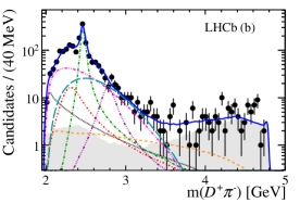
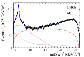
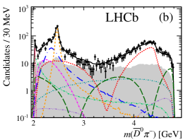
Figure 2: Projections of the data and fit models on $m(D\pi)$ for the (left) $B^{+}\to D^{-}K^{+}\pi^{-}$, (right) $B^{0}\to\overline{D}{}^{0}\pi^{+}\pi^{-}$ and (bottom) $B^{0}\to\overline{D}{}^{0}K^{+}\pi^{-}$ samples. Note that it is actually $m^{2}(D\pi)$ shown for $B^{0}\to\overline{D}{}^{0}\pi^{+}\pi^{-}$ decays.

II.3 Questions and challenges

The amplitude analysis $\Lambda^{0}_{b}\to D^{0}p\pi^{-}$ decays is currently in progress. There was some discussion about the use of model independent partial waves to model the large non-resonant contributions to $m(Dp)$. It was felt that while this approach would work, and could potentially describe the amplitude well, the results would not be portable to other analyses. This portability would be desirable when performing an amplitude analysis of the suppressed $\Lambda^{0}_{b}\to D^{0}pK^{-}$ decay, which is sensitive to the CKM angle $\gamma$.

This is also an approach being considered for the $D\pi$ S-wave in high statistics modes such as $B^{+}\to D^{-}\pi^{+}\pi^{+}$. The $D\pi$ S-wave has been described by exponential form factors in $B^{+}\to D^{-}K^{+}\pi^{-}$ and $B^{0}\to\overline{D}{}^{0}\pi^{+}\pi^{-}$ analyses, while the $B^{0}\to\overline{D}{}^{0}K^{+}\pi^{-}$ analysis used the dabba model Bugg (2009). In all cases an additional component was included for the $D^{*}_{0}(2400)$ resonance, described by a relativistic Breit-Wigner function. The combination of these functions violates unitarity, this problem could be solved with either model independent partial waves, a LASS-like approach, a K-matrix approach or the use of Veneziano-like models Veneziano (1968) as suggested by Adam Szczepaniak.

The $\pi\pi$ S-wave in $B^{0}\to\overline{D}{}^{0}\pi^{+}\pi^{-}$ was modelled using two separate methods, the isobar model and the K-matrix approach. While both of these gave good quality fits, and the results agree well between the two, it was reiterated by the theory colleagues that there are well-known problems using the isobar model the $\pi\pi$ S-wave, in particular for the $\sigma$ meson. It was also mentioned that it would be interesting to try a K-matrix approach to model the $K\pi$ S-wave.

III LHCb - CP violation in charmless $B^{\pm}$ three-body decays

Alberto C. dos Reis, for the LHCb collaboration

Centro Brasileiro de Pesquisas Físicas – CBPF
Rio de Janeiro - Brazil

III.1 Introduction

The study of CP violation (CPV) is one the main topics in contemporary particle physics. In the Standard Model (SM) CPV arises due to an irreducible phase in the Cabibbo-Kobayashi-Maskawa (CKM) matrix. All existing measurements of CP violation in decays of flavoured mesons are consistent with the SM predictions. However, the CKM mechanism for CPV fails to account for the baryon number density of the Universe by many orders of magnitude. Other sources of CPV must exist. The study of CPV, therefore, offers unique opportunities to search for new Physics, being one of the main purposes of the LHCb experiment.

The study of CPV in charmless $B$ decays is an important part of the LHCb physics programme. In this section, decays of $B^{\pm}$ mesons into three light pseudo-scalars are discussed. Four decay channels are analyzed Aaij et al. (2014b): $B^{+}\to\pi^{+}\pi^{+}\pi^{-}$, $B^{+}\to K^{+}\pi^{+}\pi^{-}$, $B^{+}\to K^{+}\pi^{+}K^{-}$ and $B^{+}\to K^{+}K^{+}K^{-}$. These processes are a primary source for studies of CPV in decay, since mixing is not possible for charged $B$ mesons.

CPV in decay occurs when a given final state may be reached by two interfering amplitudes with different weak and strong phases:

$$A=a_{1}+a_{2}\ e^{i(\delta+\gamma)},\hskip 11.38092pt\overline{A}=a_{1}+a_{2}\ e^{i(\delta-\gamma)}\ ,$$

where $\gamma$ and $\delta$ are the weak (CP odd) and strong phases (CP even) and $a_{1}$ and $a_{2}$ are real numbers. Given that $\Gamma(\bar{B}\to\bar{f})\propto|A|^{2}$ and $\Gamma(\bar{B}\to\bar{f})\propto|\overline{A}|^{2}$, the $\mathcal{A}_{CP}^{\mathrm{dir}}$ observable is

$$\mathcal{A}_{CP}^{\mathrm{dir}}\equiv\frac{\Gamma(B\to f)-\Gamma(\bar{B}\to\bar{f})}{\Gamma(B\to f)+\Gamma(\bar{B}\to\bar{f})}=\frac{2a_{1}a_{2}\sin\!\gamma\sin\!\delta}{a_{1}^{2}+a_{2}^{2}+2a_{1}a_{2}\cos\!\gamma\cos\!\delta}.$$

The weak phase difference arises from the amplitudes for the $b\to u\bar{u}s$ and $b\to s\bar{q}q$ transitions, in the case of final states with net strangeness; and $b\to u\bar{u}d$ and $b\to d\bar{q}q$, in the case of final states with zero strangeness. The advantage of charmless three-body decays results from the fact that most final states have a rich resonant structure. The interference between resonances plus the final state interactions (FSI) at the hadron level provide the required strong phase differences. These phase differences vary across the phase space and can be very large, giving rise to large CP asymmetries in specific regions of the Dalitz plot Aubert et al. (2008a); Bediaga et al. (2009, 2012).

III.2 The Dalitz plots

The Dalitz plots for the four decay channels are shown in Fig. 3. In all cases a dense, rich resonance structure is observed at low $\pi^{+}\pi^{-}$, $K^{+}\pi^{-}$ and $K^{+}K^{-}$ invariant mass squared. Since the phase space is so large, in all cases there is also a significant non-resonant component.

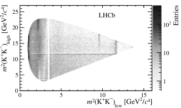
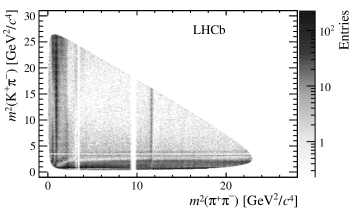
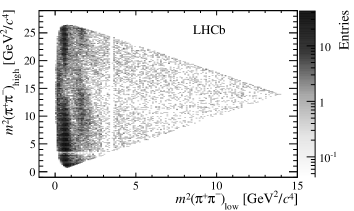
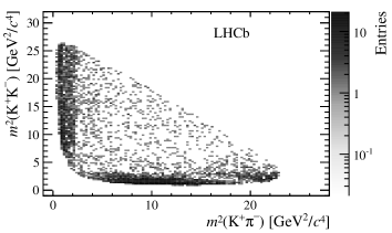
Figure 3: Dalitz plots of (top left) $K^{+}K^{+}K^{-}$, (top right) $K^{+}\pi^{+}\pi^{-}$, (bottom left) $\pi^{+}\pi^{+}\pi^{-}$ and (bottom right) $K^{+}\pi^{+}K^{-}$ candidates.

III.3 CP asymmetry across the Dalitz plot

The CP asymmetry is computed from observed signal yields:

$$A_{\mathrm{obs}}=\frac{N_{B^{-}}-N_{B^{+}}}{N_{B^{-}}+N_{B^{+}}}.$$

The CP asymmetry is obtained correcting $A_{\mathrm{obs}}$ for the $B^{\pm}$ production asymmetry and asymmetry in the detection of unpaired hadron ($B^{\pm}\to K^{\pm}h^{+}h^{-}$, $B^{\pm}\to\pi^{\pm}h^{+}h^{-}$),

$$\mathcal{A}_{CP}=A_{\mathrm{obs}}-A_{\mathrm{prod}}^{B}-A_{\mathrm{det}}^{h}\ .$$

The correction factors $A_{\mathrm{prod}}^{B}$ and $A_{\mathrm{det}}^{h}$ are determined using data-driven methods. Typical values are of the order of 1%, and are small compared to $A_{\mathrm{obs}}$. In all plots that follow we assume $A_{\mathrm{obs}}\simeq\!\mathcal{A}_{CP}$.

The Dalitz plots of the four channels are divided into bins with the same population. In each bin the value of $\mathcal{A}_{CP}$ is computed. The distribution of $\mathcal{A}_{CP}$ values in the regions $m^{2}(h^{+}h^{-})\!<\!3.5$ GeV${}^{2}/c^{4}$ is shown in Fig. 4.

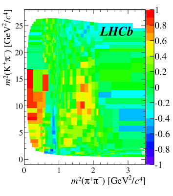
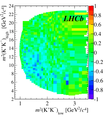
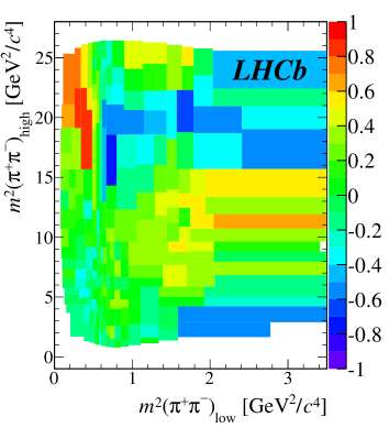
Figure 4: A zoom of the Dalitz plots of the $K^{+}\pi^{+}\pi^{-}$ (top left), $K^{+}K^{+}K^{-}$ (top right), $\pi^{+}\pi^{+}\pi^{-}$ (bottom left), $K^{+}\pi^{+}K^{-}$ (bottom right) decays, showing the distribution of $\mathcal{A}_{CP}$.

The distribution of $\mathcal{A}_{CP}$ shown in Fig. 4 exhibits some interesting features. In some regions bellow 1 GeV${}^{2}/c^{4}$ one observes values of the CP asymmetry as high as 80%, which are rather unusual. Moving from threshold to 1 GeV${}^{2}/c^{4}$ in the $K^{+}\pi^{+}\pi^{-}$ final state, the CP asymmetry changes sign as one crosses the $\rho(770)$ mass. A similar effect is visible in the $\pi^{+}\pi^{+}\pi^{-}$ Dalitz plot.

This effect may be caused by the interference between the various resonances. This hypothesis is tested with a fast simulation exercise, where the decay amplitude is represented by a sum of an S- and a P-wave component. This simple model yields a distribution of $\mathcal{A}_{CP}$ values in qualitative agreement with the experimental observations.

In the lower part of the $K^{+}\pi^{+}\pi^{-}$ Dalitz plot, the region between 1 and 2.2 GeV${}^{2}/c^{4}$ has mostly positive $\mathcal{A}_{CP}$ values. In the same region in the $K^{+}K^{+}K^{-}$ Dalitz plot one sees mostly negative $\mathcal{A}_{CP}$ values. A similar effect is observed in the $\pi^{+}\pi^{+}\pi^{-}$ and $K^{+}\pi^{+}K^{-}$ channels.

A possible interpretation of the pattern observed in the region between 1 and 2.2 GeV${}^{2}/c^{4}$ invokes CPT invariance. CPT symmetry implies equal partial widths for particle and antiparticle. As a consequence, in a family of final states sharing the same quantum numbers one must have $\sum\Gamma_{i}(B\!\to\!f_{i})=\sum\Gamma_{i}(\overline{B}\!\to\!\bar{f}_{i})$. The $K^{+}\pi^{+}\pi^{-}$ and $K^{+}K^{+}K^{-}$ channels are connected by $\pi\pi\to KK$ re-scattering, and so are the $\pi^{+}\pi^{+}\pi^{-}$ and $K^{+}\pi^{+}K^{-}$ final states. Recall that the $\pi\pi$ interaction becomes inelastic with the opening of the $K\overline{K}$ channel, and up to a center-of-mass energy of $\sim 1.5$ GeV all the inelasticity of the $\pi\pi$ interaction goes into the $K\overline{K}$ channel.

In the absence of CP violation there would be a balance between the outgoing and the ingoing flux in each channel. But if CP is violated this balance would be broken, giving rise to a positive asymmetry in one channel which must be compensated by a negative asymmetry in other channels. Of course in a comprehensive analysis of such effect one should also consider the neutral modes ($\pi^{0}\pi^{0}$ and $K^{0}\overline{K}^{0}$). But if this is the underlying mechanism of the observed CP asymmetries, then the $\pi\pi\leftrightarrow KK$ re-scattering would provide the source of the strong phase difference, a unique feature of multi-body decays. A recent studies of the impact of the $\pi\pi\leftrightarrow KK$ re-scattering can be found in Refs. Bediaga et al. (2014); Alvarenga Nogueira et al. (2015).

III.4 Challenges for the amplitude analysis

The study of CP violation in $B^{\pm}$ decays reveals an unusual pattern with large asymmetries in specific regions of the Dalitz plot. A full amplitude analysis is the necessary step towards identifying the underlying mechanisms responsible for the observed $\mathcal{A}_{CP}$ distribution. The data suggest that the hadronic degrees of freedom are the source of strong phase difference. The inclusion of the these degrees of freedom in a consistent manner is one of the main challenge of the Dalitz plot analysis of the charmless three-body $B^{\pm}$ decays.

The vast phase space of charmless three-body $B$ decays is populated by a non-resonant component. The Dalitz plot analyses of $B$ decays adopt empirical parameterizations of the non-resonant amplitude. In all cases the S-waves are a significant part of the decay amplitude. In general the S-wave includes broad structures which interfere with the smooth non-resonant component, often resulting in very large interference terms or, in other words, a sum of fit fractions that largely exceeds 100%.

A theoretical description the three-body FSI is not possible from first principles. Calculations of these FSI in the $D^{+}\!\to\!K^{-}\pi^{+}\pi^{+}$ have been performed Magalhães et al. (2011); Guimarães et al. (2014); Frederico et al. (2014), showing that this is an important effect and that a slowly varying phase is introduced. To our knowledge, no such calculation have been performed for $B$ decays.

The inclusion of re-scattering effects in the decay amplitude is a far from trivial task. This effect is entangled with the three-body re-scattering. This is another instance where input from theory is much needed.

IV LHCb - Three-body decays of charged $D$ mesons

Alberto C. dos Reis, for the LHCb collaboration

Centro Brasileiro de Pesquisas Físicas – CBPF
Rio de Janeiro - Brazil

IV.1 Introduction

Light meson spectroscopy from hadronic charm meson decays is one of the main lines of the LHCb programe on charm physics. In this section, ongoing Dalitz plot analyses of charged $D$ decays are discussed.

The very large samples of $D^{+}$ and $D^{+}_{s}$ decays into three charged light mesons offer an unique opportunity for low-energy hadron physics studies. The main motivation is the understanding of the strong dynamics of the final state, with particular emphasis on the S-wave amplitudes — a key input for CP violation studies performed with decays of $B$ mesons.

S-wave amplitudes are the dominant component in three-body $D$ decays having a pair of identical particles in the final state, such as the $D^{+}\to K^{-}\pi^{+}\pi^{+}$ and $D^{+}_{(s)}\to\pi^{-}\pi^{+}\pi^{+}$ decays Aitala et al. (2002, 2001a, 2001b); Bonvicini et al. (2007). In addition to the abundant contribution of scalar resonances, there is an unique feature of $D$ decays: the $\pi\pi$, $K\pi$ and $K\bar{K}$ scattering amplitudes can be measured throughout the whole elastic part of the spectrum, starting from threshold.

The analysis of very large data sets ($\mathcal{O}(10^{7})$ reconstructed decays in Cabibbo-suppressed modes) is rather challenging. Most Dalitz plot analyses are performed in the framework of the isobar model Asner (2003). This approach has known limitations, especially when scalar particles are involved. Going beyond the simple isobar model is indeed the major challenge. Some alternative formulations are based on the assumption that the dynamics of the final states is entirely driven by two-body interactions, disregarding any possible effect related to the third particle. It is now clear that corrections to these two-body re-scattering must be incorporated in a consistent way, using a maximum of theoretical constraints from unitarity, analycity and crossing symmetries.

IV.2 The $D^{+}_{(s)}\to\pi^{-}\pi^{+}\pi^{+}$ decays

An interesting aspect of the $\pi^{-}\pi^{+}\pi^{+}$ final state is that the $\pi^{-}\pi^{+}$ S-wave amplitude in the $D^{+}$ decay is very different from that of the $D^{+}_{s}$. The $D^{+}\to\pi^{-}\pi^{+}\pi^{+}$ decay is Cabibbo-suppressed, has a large contribution of the $\sigma$ meson and some $f_{0}(980)$. The $D^{+}_{s}\to\pi^{-}\pi^{+}\pi^{+}$ decay is Cabibbo allowed, with a large contribution of $f_{0}(980)$ and no $\sigma$. In both cases, however, there is a significant contribution of a scalar particle, referred to as “$f_{0}(X)$”, with mass between 1.4 and 1.5 GeV and width between 100 and 200 MeV (natural units are adopted). Previous determinations of the $f_{0}(X)$ parameters Aitala et al. (2001b); Link et al. (2004) indicate that this state is not consistent with neither the $f_{0}(1500)$ nor the $f_{0}(1370)$.

The combined study of the $D^{+}$ and $D^{+}_{s}$ decays provide, therefore, inputs to the physics of the light scalars, from the $\sigma$ to the $f_{0}(1710)$. The basic challenge is to extract this information. There is a consensus that one should not represent the broad, overlapping scalars as a sum of Breit-Wigner functions. Alternative approaches assume a 2+1 picture, where the dynamics of the final state is entirely determined by the two-body interaction, the third particle playing no role. One example of this approach is the recent analysis of the $B^{0}\to\overline{D}{}^{0}\pi^{+}\pi^{-}$ decay by LHCb Aaij et al. (2015b). In this work the K-matrix formalism is used for the S-wave amplitude, where the poles are obtained from a fit to the $\pi\pi$ scattering data Anisovich and Sarantsev (2003) and fixed in the Dalitz plot fit. A good description of the data is obtained, but one would like to go the other way around, that is, to extract information about $\pi\pi$ interaction from the $D$ and $B$ decays.

Another alternative is to perform a minimal model-dependent analysis, extracting the S-wave amplitude from the data making no assumption about its composition. This technique was developed by the E791 collaboration Aitala et al. (2006), and herein is referred to as ”MIPWA”. In the ”MIPWA”, the S-wave amplitude is parameterized as a generic complex function, $\mathcal{A}_{S}=a(s)e^{i\phi(s)}$ ($s\equiv m^{2}(\pi^{-}\pi^{+})$). The real functions $a(s)$ and $\phi(s)$ are obtained directly from the data, dividing the $\pi^{-}\pi^{+}$ spectrum($2m_{\pi}\!<\!m_{\pi\pi}\!<\!M_{D}-m_{\pi}$) into bins . At each bin edge, two fit parameters, $a_{k}$ and $\phi_{k}$, determine the S-wave amplitude. A spline interpolation yields the S-wave amplitude at any $m_{\pi\pi}$ value in the $\pi^{-}\pi^{+}$ spectrum. This approach was used by the BaBar collaboration in the analysis of the $D^{+}_{s}\to\pi^{-}\pi^{+}\pi^{+}$ decay Aubert et al. (2009a).

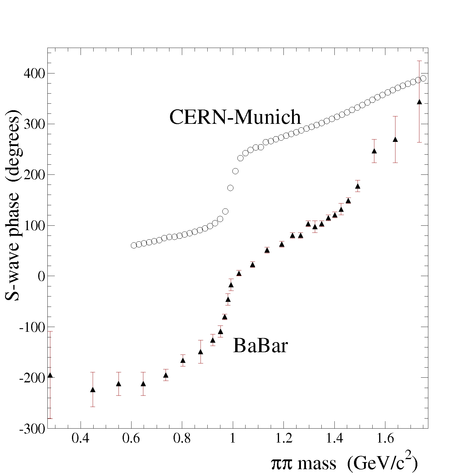
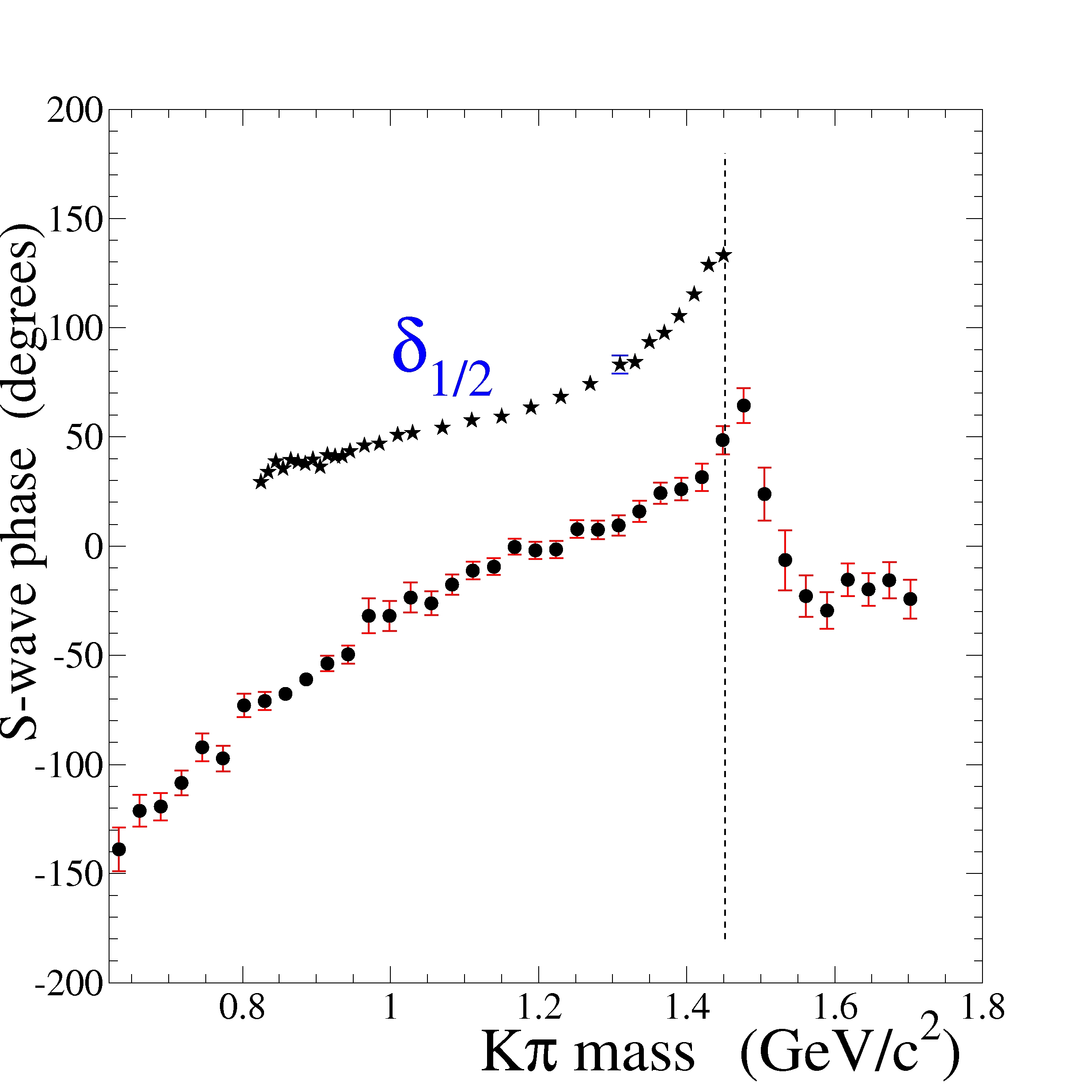
Figure 5: Left: S-wave phase from $D^{+}_{s}\to\pi^{-}\pi^{+}\pi^{+}$ Aubert et al. (2009a) and from the CERN-Munich collaboration Hyams et al. (1973); *cern-munich2. Right: S-wave phase from the FOCUS Dalitz plot analysis Link et al. (2009) of the $D^{+}\to K^{-}\pi^{+}\pi^{+}$ decay and from the LASS ($I\!=\!1/2$) experiment Aston et al. (1988a). The $K^{-}\pi^{+}\to K^{-}\pi^{+}$ cross section is elastic up to the $K\eta^{\prime}$ threshold, indicated by vertical line.

The MIPWA is probably the approach with less model dependence, relying on the assumption is that the P- and D-waves are well represented by a sum of Breit-Wigner functions. A comparison between the phases obtained by the MIPWA and those from scattering data is shown in Fig. 5. In the left panel, the S-wave phases obtained by the BaBar measurement and by the CERN-Munich collaboration Hyams et al. (1973); *cern-munich2 ($\pi^{+}\pi^{-}\to\pi^{+}\pi^{-}$) are displayed as a function of the $\pi^{+}\pi^{-}$ mass. On the right, a similar measurement of the $K^{-}\pi^{+}$ S-wave phase performed by the FOCUS collaboration Link et al. (2009) in the $D^{+}\to K^{-}\pi^{+}\pi^{+}$ decay is superimposed to the I=1/2  S-wave phase from $K^{-}\pi^{+}\to K^{-}\pi^{+}$ scattering obtained by the LASS collaboration Aston et al. (1988a).

The differences between the S-wave phases obtained from $D$ decays and from scattering data are evident, which seems to indicate deviations from Watson’s final-state theoremWatson (1952). In addition to an overall shift, in both $\pi^{+}\pi^{-}$ and $K^{-}\pi^{+}$ systems there is a clear mismatch between the phase motion from decay and scattering. This discrepancy indicates that other effects must be taken into account.

One can picture the decay of a $D$ meson as a time-ordered sequence of the short-distance $c$ quark transition, resulting in the ”final state quarks”, from which the long-distance hadronization occurs. The different configuration of the final state quarks would explain the differences in the S-wave composition in the $D^{+}$ and $D_{s}^{+}$ decays described above. Strong phases, possibly with some smooth energy dependence, may be generated in the ”weak vertex”, and would depend on the nature of the initial $D$ meson. The hadrons emerging from the weak vertex re-scatter in all possible ways before reaching the detector: $D\to KK\bar{\pi}\to\pi\pi\pi$, $D\to K^{0}\pi^{0}\pi\to K^{-}\pi^{+}\pi$, three-body interactions. Studies performed with the $D^{+}\to K^{-}\pi^{+}\pi^{+}$ decay Magalhães et al. (2011); Guimarães et al. (2014); Frederico et al. (2014); Magalhães and Robilotta (2015) show that FSI involving all three particles in hadronic loops are an important effect, explaining part of the differences in the S-wave phases observed in Fig. 5.

The S-wave phases measured with the MIPWA technique must be understood as a convolution of the pure, universal $\pi^{+}\pi^{-}$/$K^{-}\pi^{+}$ scattering phases with those inherited from the weak vertices and with phases resulting from three-body FSI. Moreover, in $D$ decays one cannot disentangle the contribution from the different isospin amplitudes. In addition, given the large number of free parameters, any defect on the representation of the other waves will leak into the MIPWA phase.

A comparative study of the MIPWA $\pi^{+}\pi^{-}$ S-wave amplitude in $D^{+}$ and $D^{+}_{s}\to\pi^{-}\pi^{+}\pi^{+}$ decays is very important. The mass difference between the $D^{+}$ and the $D^{+}_{s}$ is only 100 MeV. This may be seen as a bonus: three-body FSI should be similar in the $D^{+}$ and the $D^{+}_{s}$ decays. A comparison between measurements of the raw S-wave phases would provide information about the $D^{+}$ and $D^{+}_{s}$ weak vertices. This should be taken with a grain of salt, though, since it is not really possible to draw a clear line separating classes of FSI.

In a model-dependent measurement, different line shapes of the $\sigma$ meson can be tested. A simultaneous study of the S-wave amplitude from the $D^{+}$ and $D^{+}_{s}$ decays will give information about the scalar meson at $\sim$1.4 GeV. Isospin-breaking processes can also be addressed in model-dependent measurements. A precise determination of the $f_{0}(980)$ line shape, possible in the $D^{+}_{s}$ decay, is related to the physics of the $f_{0}-a_{0}$ mixing. This effect is enhanced in the region between the $K^{+}K^{-}$ and $K^{0}\bar{K}^{0}$ thresholds Achasov et al. (1979). These thresholds are 8 MeV apart, while the LHCb mass resolution is of the order of 2 MeV. The $\rho-\omega$ mixing can be studied in the $D^{+}$ decay, where a large $\rho(770)^{0}\pi^{+}$ contribution is observed.

Model-dependent and MIPWA measurements are under way in LHCb. For the $D^{+}$ decay the MIPWA measurements of the $\pi^{+}\pi^{-}$ S-wave amplitude will be made for the first time. For the $D^{+}_{s}$ decay a significant improvement in precision is expected, since the LHCb sample is one order of magnitude larger than that of BaBar.

IV.3 The $D^{+}_{(s)}\to K^{-}K^{+}\pi^{+}$ decays

Another ongoing effort in the LHCb charm physics programme is the study of the $D^{+}_{(s)}\to K^{-}K^{+}\pi^{+}$ decays. The main goal is the MIPWA measurement of the $K^{+}K^{-}$ S-wave amplitude, an important input to CP violation studies in the $B$ meson system. Statistics is not an issue: the selected $D^{+}_{(s)}\to K^{-}K^{+}\pi^{+}$ sample is approximately ten times larger than that of $D^{+}_{(s)}\to\pi^{-}\pi^{+}\pi^{+}$, with much higher purity due to the presence of two kaons. Compared to BaBar, the LHCb $D^{+}_{(s)}\to K^{-}K^{+}\pi^{+}$ signals are two orders of magnitude larger. The major challenge for the MIPWA measurement of the $K^{+}K^{-}$ S-wave is the presence of an S-wave component also in the $K^{-}\pi^{+}$ system. Both amplitudes populate the whole phase space. The best strategy for this measurement needs still to be defined. As in the case of the $\pi^{-}\pi^{+}\pi^{+}$ final state, a model-dependent analysis is also underway.

The $D^{+}\to K^{-}K^{+}\pi^{+}$ is a Cabibbo-suppressed decay. There are two tree-level diagrams leading to $(K\pi)^{0}K^{+}$ and to $(K\bar{K})^{0}\pi^{+}$ intermediate states. Contributions from resonances coupling to both $K^{-}\pi^{+}$ and $K^{-}K^{+}$ are therefore expected.

The $D^{+}_{s}\to K^{-}K^{+}\pi^{+}$ decay is Cabibbo-allowed. As for the $D^{+}$, there are two tree-level diagrams. The colour suppressed can lead to both $K^{-}\pi^{+}$ and $K^{-}K^{+}$ resonances, whereas the colour allowed (external W-radiation) leads mainly to $K^{+}K^{-}$ resonances. The latter is the same as for the $D^{+}_{s}\to\pi^{-}\pi^{+}\pi^{+}$, so a strong contribution of the $f_{0}(980)\pi^{+}$ is expected, as well as a large $\phi\pi^{+}$ component. In the model-dependent analysis, the coupling of the $f_{0}(980)$ to $K\bar{K}$ can be measured independently in the $K^{-}K^{+}\pi^{+}$ and $\pi^{-}\pi^{+}\pi^{+}$ final states.

In both $D^{+}$ and $D^{+}_{s}$ decays there is a tree-level diagram with an $s\bar{s}$ pair which could form resonances of the $f_{0}$ family with mass above 1 GeV, including the $f_{0}(X)$ state. The situation concerning these resonances and their contribution to $D$ and $B$ decays is still rather confuse. The measurement of the $K^{-}K^{+}$ S-wave amplitude will help to understand the role — and the nature — of these states in heavy flavour decays.

V LHCb - Exotic hadron spectroscopy

Tomasz Skwarnicki, for the LHCb collaboration

Syracuse University
Syracuse, New York, USA

The LHCb experiment offers unique opportunities in the field of exotic hadron spectroscopy. Production rates of $B$ mesons are 3 orders of magnitude larger than previously available at the $e^{+}e^{-}$ $B$ factories (Belle and BaBar). Even after correcting for the smaller reconstruction efficiencies, LHCb has typically collected 10 times bigger data samples of $B$ meson decays to $J/\psi$ and light-quark hadrons in all charged particle final states during Run I at LHC (2011-12, 3 fb^-1). The long visible lifetime of the lightest $b$-hadrons provides for excellent suppression of combinatorial backgrounds and two RICH detectors provide further background suppression for final states with at least one charged kaon. Thus, signal-to-background ratios have been slightly better than those at the $e^{+}e^{-}$ $B$ factories. The RICH detectors, and the large trigger bandwidth to tape (up to 5 kHz at Run I) devoted almost entirely to the flavor physics offer a competitive edge over the general purpose detectors, ATLAS and CMS. The larger $b\bar{b}$ cross-section at the LHC as compared to the Tevatron, offers additional advantage over the CDF and D0 data samples. A unique advantage over the $e^{+}e^{-}$ $B$ factories comes with simultaneous productions of $B$, $B_{s}$, $B_{c}$ mesons and $b-$quark baryons ($B_{s}$ samples require dedicated beam time at the $B$ factories, while $B_{c}$ and $b-$baryons are not accessible). The efficient trigger on final states with the $J/\psi\to\mu^{+}\mu^{-}$ decays led to several high impact results in the field of exotic hadrons related to the charmonium family. The same final states offer also an opportunity to study conventional and exotic light-hadron spectroscopy in a relatively clean environment as illustrated in Ref. Aaij et al. (2014c).While this potential of the LHCb experiment has gone largely unexplored, we concentrate here on exotic spectroscopy with heavy charmed quarks inside. The dominant weak decays turn a $b$ quark to a $c$ quark, while a companion $\bar{c}$ comes from the associated $W\to\bar{c}s$ vertex.

Three LHCb amplitude analyses are worth invoking here. The use of full angular phase-space (5D) in the analysis of the $X(3872)$ decays to $\rho^{0}J/\psi$, with $\rho^{0}\to\pi^{+}\pi^{-}$ and $J/\psi\to\mu^{+}\mu^{-}$, with the fully polarized $X(3872)$ states produced in $B^{+}\to X(3872)K^{+}$ decays, led to the first decisive determination of $X(3872)$ spin and parity ($J^{P}=1^{+}$) Aaij et al. (2013a), in a sample not much larger than previously available in Belle, where an opportunity to achieve such a goal earlier was missed due to the limitations of three 1D angular fits which were employed. This example underscores the importance of studying full decay dynamics especially when number of signal events is limited. An update to this analysis published recently, confirmed these results without any assumptions about the orbital angular momentum in the $X(3872)\to\rho^{0}J/\psi$ decays and set a tight upper limit on the $D$-wave fraction Aaij et al. (2015d). This assignment of quantum numbers ruled out the closest-in-mass $c\bar{c}$ hypothesis ($\eta_{c}(2^{3}D_{2^{-+}})$). The remaining explanations invoke either a loosely bound $D^{0}\overline{D}^{*0}$ molecule, which would explain the mass coincidence with the $D^{0}\overline{D}^{*0}$ threshold, the $\chi_{c}(2^{3}P_{1^{++}})$ conventional meson or a tightly bound $(cu)(\bar{c}\bar{d})$ tetraquark, attracted to the threshold via quantum effects Bugg (2008) (for a recent review see Ref. Esposito et al. (2014)). The $X(3872)$ is too narrow to be simply a $D^{0}\overline{D}^{*0}$ cusp, with no bound state contribution Bugg (2008).

The 4D amplitude analysis of $B^{0}\to\psi^{\prime}\pi^{+}K^{-}$ decays, had less angular dimensions to work with, but many conventional $K^{*0}$ states contributing to the observed $\pi^{+}K^{-}$ mass distribution. A successful amplitude model was found, which required a very significant ($>13\sigma$) contribution of the exotic $Z(4430)^{+}$ state decaying to $\psi^{\prime}\pi^{+}$ (see Fig. 6) Aaij et al. (2014d).This state was first observed by Belle Choi et al. (2008), but was in experimental limbo for many years after the BaBar experiment was not able to confirm it Aubert et al. (2009b). The LHCb results agree very well with the results of the earlier Belle 4D amplitude analysis of the same channel Chilikin et al. (2013) on the $Z(4430)^{+}$ mass, width and fit fraction, while improving their determination. The $3.4\sigma$ evidence for $J^{P}=1^{+}$ assignment to $Z(4430)^{+}$ from Belle, was also confirmed beyond any doubt. Last but not least, thanks to a sample 10 times larger than that available at Belle, LHCb was able to probe $Z(4430)^{+}$ amplitude dependence on $\psi^{\prime}\pi^{+}$ mass without the Breit-Wigner assumption. The resulting Argand diagram (Fig. 7) shows a quick counter-clockwise change of the amplitude phase at the peak of its magnitude, in agreement with the resonant hypothesis. This diagram rules out the rescattering model by Pakhlov-Uglov Pakhlov and Uglov (2015), offered as an explanation for the $Z(4430)^{+}$ mass peak, since it predicts the phase mass running in the opposite direction.

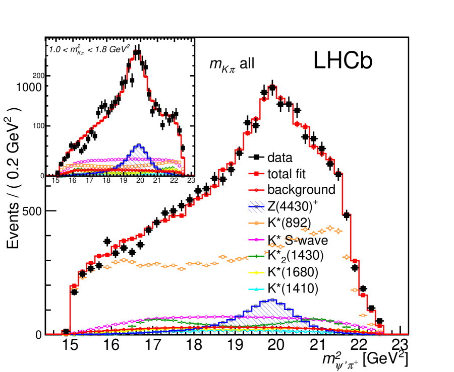
Figure 6: Distribution of invariant mass of $\psi^{\prime}\pi^{+}$ squared for $B^{0}\to\psi^{\prime}\pi^{+}K^{-}$, $\psi^{\prime}\to\mu^{+}\mu^{-}$ candidates together with the projections of the 4D fit of $K^{*0}\to K^{-}\pi^{+}$ and $Z(4430)^{+}\to\psi^{\prime}\pi^{+}$ amplitudes. The distribution for the $K^{-}\pi^{+}$ mass slice in which the $K^{*0}$ contributions are smaller is shown in the inset.

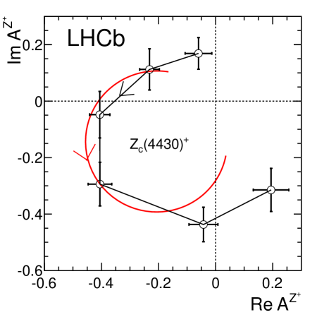
Figure 7: Fitted values of the real and imaginary parts of the amplitude for the $Z(4430)^{+}$ state divided into six $m_{\psi^{\prime}\pi}^{2}$ bins of equal width between $18.0$ and $21.5$ GeV² range, shown in the Argand diagram as connected points with the error bars ($m_{\psi^{\prime}\pi}^{2}$ increases counterclockwise). The solid (red) curve is the prediction from the Breit-Wigner formula with a resonance mass (width) of 4475 (172) $\mathrm{MeV}$and magnitude scaled to intersect the bin with the largest magnitude centered at (4477 MeV)². The phase convention assumes the helicity-zero $K^{*}(892)$ amplitude to be real. Systematic uncertainties are not included.

The 6D amplitude analysis of $\Lambda_{b}\to J/\psi pK^{-}$ decays Aaij et al. (2015e) followed in footsteps of the $B^{0}\to\psi^{\prime}\pi^{+}K^{-}$ analysis. The increased dimensionality is due to the $\Lambda_{b}$ spin. The observed $J/\psi p$ mass distribution, which contains a narrow peak at 4450 $\mathrm{MeV}$, could not be described with the excitations of the $\Lambda$ baryon. Two interfering $J/\psi p$ resonances of opposite parity with allowed spin combinations being either ($3/2$, $5/2$) or ($5/2$, $3/2$) are needed, in addition to the known $\Lambda^{*}$ resonances, for a successful description of the data (see Fig. 8). The two new states have been labeled $P_{c}(4380)^{+}$ and $P_{c}(4450)^{+}$ with the lighter one having a larger width of $218\pm 18\pm 86$ $\mathrm{MeV}$then the heavier one, which is very narrow for a resonance at such high mass, $39\pm 5\pm 19$ $\mathrm{MeV}$. The Argand diagram for the narrower state is very consistent with the resonant behavior and is inconclusive for the broader state (Fig. 9). The pair can be accommodated in the diquark model of tightly bound pentaquarks, via a change of the orbital angular momentum between the states, which explains the opposite parity and the prediction that the narrower state has a spin of $5/2$, which also would explain its smaller width due to the orbital angular momentum barrier factor in its decay Maiani et al. (2015); Lebed (2015); Anisovich et al. (2015). While the narrower state can be accommodated as a baryon-meson molecule, either $\Sigma D^{*0}$ Karliner and Rosner (2015); Chen et al. (2015); Roca et al. (2015); He (2015) or $p\chi_{c}(1P_{1})$ Meißner and Oller (2015), if its spin is $3/2^{-}$, the $5/2$ spin cannot be reached in the molecular model since $l=1$ molecular states are very unlikely to be bound. Rescattering models have been also proposed Guo et al. (2015); Liu et al. (2015); Mikhasenko (2015); Szczepaniak (2015a). While they can produce the peak at the $P_{c}(4450)^{+}$ mass, with the counterclockwise running of phase with the mass, it is not yet clear whether they can produce fits as good as those achieved from assuming bound state models in all 6 dimensions. Such mechanisms cannot produce a structure with a spin of $5/2$ at these masses.

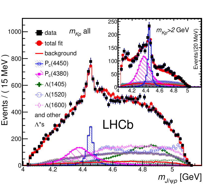
Figure 8: Distribution of invariant mass of $J/\psi p$ for $B^{0}\to J/\psi pK^{-}$, $J/\psi\to\mu^{+}\mu^{-}$ candidates together with the projections of the 6D fit of $\Lambda^{*}\to K^{-}p$ and $P_{c}^{+}\to J/\psi p$ amplitudes. The distribution for the $K^{-}p$ mass slice in which the $|Lambda^{*}$ contributions are smaller is shown in the inset.

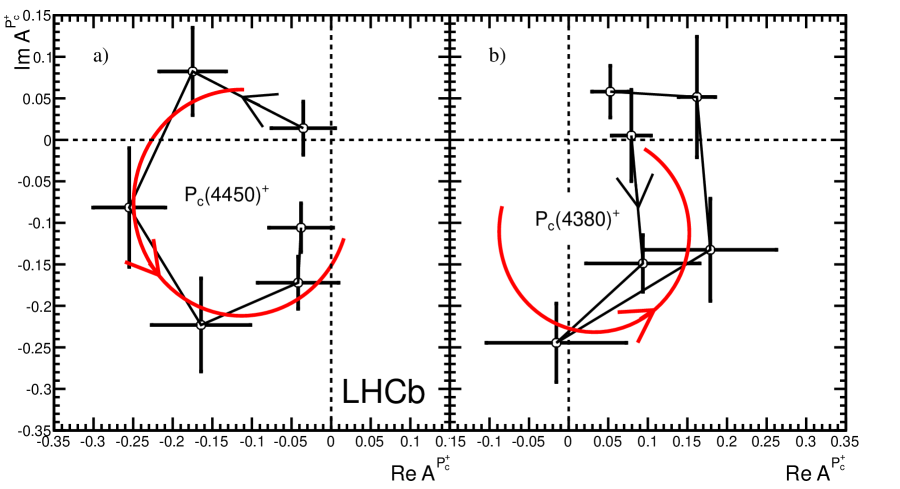
Figure 9: Fitted values of the real and imaginary parts of the amplitudes for the baseline ($3/2^{-}$, $5/2^{+}$) fit for a) the $P_{c}(4450)^{+}$ state and b) the $P_{c}(4380)^{+}$ state, each divided into six $m_{J/\psi p}$ bins of equal width between $-\Gamma_{0}$ and $+\Gamma_{0}$ shown in the Argand diagrams as connected points with error bars ($m_{J/\psi p}$ increases counterclockwise). The solid (red) curves are the predictions from the Breit-Wigner formula for the same mass ranges with $M_{0}$ ($\Gamma_{0}$) of 4450 (39) $\mathrm{MeV}$and 4380 (205) $\mathrm{MeV}$, respectively, with the phases and magnitudes at the resonance masses set to the average values between the two points around $M_{0}$. The phase convention assumes $L=0$, $S=\frac{1}{2}$ amplitude for $\Lambda(1520)$ to be real. Systematic uncertainties are not included.

While the $P_{c}^{+}$ states are the first plausible pentaquark candidates with heavy quarks inside, there are many other observed neutral and charged tetraquark candidates with a $c\bar{c}$ pair inside (the neutral exotic candidates could also be hybrid states), but not necessarily confirmed, by the other experiments (see e.g. Ref. Esposito et al. (2014)). Although many such states have been reported, including several $Z_{b}^{+}$ candidates, no clear theoretical model explaining all of them has emerged. The main competitors are tightly bound tetraquark and pentaquark models with diquarks inside, molecular models and rescattering processes. Once at work for one phenomenon (e.g. for the $P_{c}^{+}$ pentaquark candidates), the same mechanism should also be at work at other masses, different multiquark structures (e.g. also for tetraquarks) and with different quark flavor structure (isospin and SU(3)_f partners, $b\bar{b}$ and $c\bar{c}$ etc.). In fact, different bound state models lead to different but always rich “periodic tables” of various expected states. Uncovering new entries to the experimentally observed tables is of crucial importance. However, it is also possible that more than one dynamics is at play for multiquark systems, which would vastly complicate the interpretation of the data.

Exotic bound states are likely to decay to more than one mode, and could be produced by more than one process (e.g. prompt production, central-exclusive production, heavy ion collisions). Each observation contributes a new insight into internal hadron structure. Rescattering processes are likely to produce structures which are specific for each final state and each production mechanism. Thus searches for the known exotic states in different decay modes or in different production environment are doubly important.

The opportunities for experimental advancement of exotic hadron spectroscopy in LHCb are, therefore, very rich and likely will be manpower limited for foreseeable future. Many channels known to contain important information, even easily accessible in LHCb like $B^{0}\to J/\psi\pi^{+}K^{-}$, await thorough amplitude analysis. Other, harder to access channels, like $\chi_{cJ}\pi^{+}K^{-}$ will have lower statistics and worse purity but are still usable for the important goal of verifying the states claimed in these channels by other collaborations. Survey of all accessible channels, especially in b-baryon decays, in a hunt for new entries to the pentaquark candidate tables and for the existing ones in new decay modes or new production mechanisms, is an important responsibility for the LHCb collaboration given its unique experimental capabilities in this area. Search for even more complex multiquark structures, like hexaquarks (among them dibaryons) is also a unique window of opportunity. Theoretical guidance has been already provided by specific models, but open minded searches should be performed too.

Refining the analysis of the decays that already produced important results ($Z(4430)^{+}$ and $P_{c}^{+}$ states) should not be forgotten. Increased data statistics from the on-going Run II, and later from the upgraded LHCb, will help this goal. However, even the existing data samples may contain more information than already extracted. For example, the exotic hadron structures cross many conventional resonances. Careful investigation of their interference patterns in different parts of the Dalitz plane may provide firmer evidence for their bound state nature or indicate rescattering processes.

The LHCb detector is equipped with a trigger on purely hadronic final states with a detached secondary vertex. Such triggers have been successfully utilized to study $D(s)$ meson spectroscopy from $B(s)^{0}\to DK^{+}\pi^{-}$ and $D\pi^{+}\pi^{-}$ final states Aaij et al. (2014e, a, 2015b, 2015a). Such studies are also important for interpretation of exotic hadron candidates. For example, the only remaining molecular explanation of the $Z(4430)^{+}$ state is a $D\,\overline{D}(2600)$ hypothesis. This calls for confirmation of the $D(2600)$ state and determination of its quantum numbers ($1^{-}$ has been assumed). With larger future data samples, a possibility of tetraquarks with one $c$ quark inside can perhaps be also explored. Work on conventional states that constitute “background” components to the exotic candidates, like e.g. $K^{*}$ states in decays to $K\pi$ and $\phi K$, or $\Lambda^{*}$ states in decays to $Kp$ using the other channels than the ones known to contain strong exotic signals in the coupled decay mode is likely to be important for future precision amplitude fits.

The theoretical community already provides plenty of guidance concerning possible interpretation of the existing exotic hadron candidates, as well as prediction for other channels and states to look for. It would be very useful to see more theoretical work on ways to distinguish rescattering signals from true bound states. At present the rescattering papers play the role of spoilers, providing post-dictions offering mundane explanation of the observed peaks. Promoting them to models with predictive power would be useful. The sensitivity of high statistics amplitude analyses may become limited by theoretical limitations of the frameworks employed in fitting the data. So far, the amplitude analyses in LHCb with exotic hadron components relied on isobar approximation in spite of its known limitations. Theorists can help design variations of this framework to expose the limitations of such approach. The other known problem is how to describe very broad, often referred to as “non-resonant”, contributions. Since the amplitude analyses involving exotic candidates involve final particles with spin, theoretical works assuming final particles with no spin are not terribly useful.

The analysis of angular moments in the conventional hadron channel, reflected into mass distribution in the coupled exotic channel, motivated by the past BaBar papers, has been also employed in LHCb and promoted to proper statistical analysis in the $B^{0}\to\psi^{\prime}\pi^{+}K^{-}$ channel Aaij et al. (2015f). Such a method can also be employed in the analysis of other final states, though its sensitivity is limited to prominent exotic peaks. At best it proves a need for exotic (or rescattering) contributions. Negative outcomes do not carry useful information, as the sensitivity of this method cannot be evaluated without an amplitude model. In fact, there is a danger of misinterpretation of null results, thus this method must be applied with proper awareness of its limitation. When the outcome is positive, then the results are very valuable, but the amplitude analysis is still absolutely necessary for the interpretation of the exotic structures. Suggestions for other alternative ways of analyzing multidimensional data with coupled conventional and exotic decay channels may be helpful.

VI LHCb - Four body decays of $D$ mesons

Sam Harnew & Jonas Rademacker, for the LHCb collaboration

H. H. Wills Physics Laboratory, University of Bristol,
Bristol, United Kingdom

VI.1 Formalism and differences to three body decays

The differential decay rate of a $D$ meson into a final state $f$ of $N_{f}$ pseudoscalars with four momenta $p_{1},\ldots,p_{N_{f}}$ is given by,

$$\mathrm{d}\Gamma[{D}\to f(\mathbf{x})]=\left|\mathcal{M}(\mathbf{x})\right|^{2}\left|\frac{\partial^{n}{\boldsymbol{\phi}(\mathbf{x})}}{\partial(x_{1},\ldots,x_{n})}\right|\mathrm{d}^{n}x,$$ (1)

where $\mathcal{M}$ is the matrix element describing the ${D}\to f$ transition and $|\frac{\partial^{n}{\boldsymbol{\phi}(\mathbf{x})}}{\partial(x_{1},\ldots,x_{n})}|$ represents the density of states at point $\mathbf{x}=(x_{1},\ldots,x_{n})$ in $n$ dimensional phase space, with $n=3N_{f}-7$. For $N_{f}=3$, this leads the important case of the two-dimensional Dalitz plot, discussed much in these proceedings, and usually parametrised with $s_{12}=(p_{1}+p_{2})^{2}$ and $s_{23}=(p_{2}+p_{3})^{2}$. For $N_{f}=4$, phase space is five dimensional. Five independent variables analogous to $s_{12}$ and $s_{23}$ can be formed by combining and squaring different final state 4-momenta. However, such variables cannot fully describe four-body decay kinematics. The reason for this is related to the way in which three and four body decays transform under parity. In the decay of a pseudoscalar to three pseudoscalars, the daughters’ four-momenta form a plane in the mother’s center-of-mass frame; for this reason the effect of the parity operation can also be achieved by a rotation. Hence there can be no parity violating observables in such decays and it is indeed possible to parametrise their kinematics using the parity-invariant observables $s_{12}$ and $s_{23}$. In 4-body decays, where the daughters are no longer constrained to a plane, parity violating observables can be defined, and the decay cannot be fully described using only parity-invariant parameters. Although this might seem like an unwelcome complication, it also means that four-body decays provide a new set of parity-odd observables. These have unique sensitivity to $C\!P$ violation, as discussed in Section VI.3.2.

Usually, $\mathcal{M}$ is modelled using a coherent sum of decay amplitudes, where each proceeds via a sequence of resonant two-body decays. The theoretical limitations of this approach are discussed in detail elsewhere in these proceedings. The amplitude structure of four body decays is significantly more complicated than in three-body decays, since there are usually two resonances in each decay sequence, and there is a much larger variety of possible spin/helicity structures. This complication also leads to another benefit of four-body decays: while decays of a pseudoscalar to three pseudoscalars can only contain intermediate resonances with natural spin-parity ($J^{P}=0^{+},1^{-},2^{+},\ldots$), there is no such restriction for four-body decays.

Four body amplitude analyses have for example been carried out in ${{D}^{0}}\to K^{-}\pi^{+}\pi^{-}\pi^{+}$, ${{D}^{0}}\to{{\kern 1.99997pt\overline{\kern-1.99997ptK}{}}{}^{0}}\pi^{+}\pi^{-}\pi^{0}$, ${{D}^{+}}\to K^{-}\pi^{+}\pi^{+}\pi^{0}$, ${{D}^{+}}\to{{\kern 1.99997pt\overline{\kern-1.99997ptK}{}}{}^{0}}\pi^{+}\pi^{+}\pi^{-}$, ${{D}^{0}}\to K^{-}K^{+}\pi^{-}\pi^{+}$, ${{D}^{0}}\to K^{-}K^{-}K^{+}\pi^{+}$, and ${{D}^{0}}\to\pi^{-}\pi^{+}\pi^{-}\pi^{+}$ by the MARK III, FOCUS and CLEO collaborations Coffman et al. (1992); Link et al. (2005a, 2007, 2003); Artuso et al. (2012). In this article, we focus on the use of 4-body charm decays for $C\!P$ violation measurements, and the role of amplitude models in this context.

VI.2 Measurement of the $C\!P$-violating phase $\gamma$

VI.2.1 Formalism

One of the key applications of an amplitude model is in the measurement of the $C\!P$ violating phase $\gamma$ (or $\phi_{3}$) in $B^{-}\to{D}_{B^{-}}K^{-}$ decays (and similar) where ${D}_{B^{-}}$ represents the following superposition of ${D}^{0}$and ${\kern 1.99997pt\overline{\kern-1.99997ptD}{}}{}^{0}$:

$${D}_{B^{-}}\propto{{D}^{0}}+r_{B}e^{i(\delta_{B}-\gamma)}{{\kern 1.99997pt\overline{\kern-1.99997ptD}{}}{}^{0}}.$$ (2)

Here $r_{B}$ is the magnitude of the ratio of the $B^{-}\to{{D}^{0}}K^{-}$ to $B^{-}\to{{\kern 1.99997pt\overline{\kern-1.99997ptD}{}}{}^{0}}K^{-}$ amplitude, and $\delta_{B}$ is the a $C\!P$–conserving phase generated by the strong interaction. The phase difference $(\delta_{B}-\gamma)$ between the two decay amplitudes can be measured in decays of ${D}_{B^{-}}$ to a final state $f$ accessible from both ${D}^{0}$ and ${\kern 1.99997pt\overline{\kern-1.99997ptD}{}}{}^{0}$ Gronau and Wyler (1991); Gronau and London (1991); Atwood et al. (1997); Giri et al. (2003); Poluektov et al. (2004a). Performing the measurment in both $B^{-}\to{D}_{B^{-}}K^{-}$ and its $C\!P$-conjugate decay mode allows to disentangle $\delta_{B}$ and $\gamma$. The ${D}_{B^{-}}$ decay rate at phase space point $\mathbf{x}$ can be expressed in terms of the ${D}^{0}$ and ${\kern 1.99997pt\overline{\kern-1.99997ptD}{}}{}^{0}$ amplitudes $\mathcal{A}_{f}(\mathbf{x})$ and $\bar{\mathcal{A}}_{f}(\mathbf{x})$ as

$$\Gamma_{{D}_{B^{-}}}\propto\left|\mathcal{A}_{f}(\mathbf{x})\right|^{2}+r_{B}^{2}\left|\bar{\mathcal{A}}_{f}(\mathbf{x})\right|^{2}+r_{B}\left|\mathcal{A}_{f}(\mathbf{x})\bar{\mathcal{A}}_{f}(\mathbf{x})\right|\cos(\delta_{B}-\gamma-\delta(\mathbf{x}))$$ (3)

where $\delta(\mathbf{x})\equiv\arg(\mathcal{A}_{f}(\mathbf{x})\bar{\mathcal{A}}^{*}_{f}(\mathbf{x}))$. To determine $\gamma$ requires information on both the magnitude of $\mathcal{A}_{f}(\mathbf{x})$ and $\delta(\mathbf{x})$. While $\left|\mathcal{A}_{f}(\mathbf{x})\right|^{2}$ can be taken directly from ${{D}^{0}}\to f$ data accessible at the B-factories or LHCb, obtaining $\delta(\mathbf{x})$ is more challenging. One approach is to use an amplitude model to obtain the phase information from a fit ${{D}^{0}}\to f$ and ${{\kern 1.99997pt\overline{\kern-1.99997ptD}{}}{}^{0}}\to f$ data. This model-dependent approach has been used successfully to constrain gamma using three-body decays, e.g. Aubert et al. (2005, 2008b); Poluektov et al. (2004b, 2006); Aaij et al. (2014f). With current datasets at LHCb, it should be possible to reach a similar precision with four-body final states such as ${K^{+}}K^{-}{\pi^{+}}{\pi^{-}}$ and ${\pi^{+}}{\pi^{-}}{\pi^{+}}{\pi^{-}}$ Rademacker and Wilkinson (2007).

VI.2.2 Model-independent measurement of the $C\!P$-violating phase $\gamma$

The theoretical limitations of the most widely-used amplitude models are a key topic discussed in several contributions to these proceedings. As a result of these limiations, the model-dependent approach discussed above suffers from significant systematic uncertainties. This motivates the use of model-independent methods.

The model-independent methods discussed here are based on data-driven techniques that split phase space into one or more regions and integrate over these regions. In phase space region $i$ one can define the complex interference parameter,

$$Z^{f}_{i}=\frac{\int_{\mathbf{x}\in i}\mathcal{A}_{f}(\mathbf{x})\bar{\mathcal{A}}^{*}_{f}(\mathbf{x})\left|\frac{\partial^{n}{\boldsymbol{\phi}(\mathbf{x})}}{\partial(x_{1},\ldots,x_{n})}\right|\mathrm{d}^{n}x}{\sqrt{\int_{\mathbf{x}\in i}\left|\mathcal{A}_{f}(\mathbf{x})\right|\left|\frac{\partial^{n}{\boldsymbol{\phi}(\mathbf{x})}}{\partial(x_{1},\ldots,x_{n})}\right|\mathrm{d}^{n}x\;\int_{\mathbf{x}\in i}\left|\bar{\mathcal{A}}_{f}(\mathbf{x})\right|^{2}\left|\frac{\partial^{n}{\boldsymbol{\phi}(\mathbf{x})}}{\partial(x_{1},\ldots,x_{n})}\right|\mathrm{d}^{n}x}}.$$ (4)

In this region of phase space the $\gamma$-sensitive interference term in $B^{-}\to({D}\to f)K^{-}$ decays is proportional to $|Z^{f}_{i}|\cos(\delta_{B}-\gamma-\arg(Z^{f}_{i}))$. The parameter $Z^{f}_{i}$ is equivalent to the coherence factor $R_{i}^{f}$ and average strong phase difference $\delta_{i}^{f}$ introduced in Atwood and Soni (2003), and the $c_{i}$ and $s_{i}$ parameters introduced in Giri et al. (2003) through $Z^{f}_{i}=R_{i}^{f}e^{-i{\delta_{i}^{f}}}=c_{i}+s_{i}$ (where we follow Bondar and Poluektov (2006) for the normalisation of $c_{i},s_{i}$). The phase of $Z^{f}_{i}$ is a weighted average of $\delta(\mathbf{x})$ over $i$, and $|Z^{f}_{i}|\in[0,1]$ describes the dilution of the interference term from integrating over $i$. The advantage of this binned approach is that $Z^{f}_{i}$ can be measured amplitude-model-independently, using decays of well-defined superpositions of ${{D}^{0}}$ and ${{\kern 1.99997pt\overline{\kern-1.99997ptD}{}}{}^{0}}$, accessible at the charm threshold and in charm mixing Giri et al. (2003); Bondar and Poluektov (2006); Atwood and Soni (2003); Harnew and Rademacker (2014, 2015).

Somewhat paradoxically, input from an amplitude model is still important to maximise the sensitivity of model-independent analyses. With a model it is possible to select regions of phase space such that $|Z^{f}_{i}|$, which multiplies the $\gamma$-sensitive term, is as large as possible Bondar and Poluektov (2007). Any inaccuracies in the model will not lead to a systematic bias, but just a reduction in $|Z^{f}_{i}|$, and a corresponding reduction in sensitivity, which will be apparent in the statistical uncertainty. The same model-informed, model-unbiased constraints on $Z^{f}_{i}$ provide valuable input to time-dependent mixing and $C\!P$ violation measurements in the ${{D}^{0}}-{{\kern 1.99997pt\overline{\kern-1.99997ptD}{}}{}^{0}}$ system Bondar et al. (2010); Malde and Wilkinson (2011); Aaij et al. (2015g).

VI.2.3 Quantum correlated $\psi(3770)\to{{D}{\kern 1.99997pt\overline{\kern-1.99997ptD}{}}}$ decays

Quantum correlated $\psi(3770)\to{{D}{\kern 1.99997pt\overline{\kern-1.99997ptD}{}}}$ decays provide the well-defined ${{D}^{0}}-{{\kern 1.99997pt\overline{\kern-1.99997ptD}{}}{}^{0}}$ superpositions needed to measure $Z^{f}_{i}$. For example if one $D$ meson (the ‘tag’) decays to a $C\!P$ $\pm$ eigenstate, then the other must be in the following superposition (using the convention that $C\!P{{D}^{0}}=+{{\kern 1.99997pt\overline{\kern-1.99997ptD}{}}{}^{0}}$):

$${D}\propto{{D}^{0}}\mp{{\kern 1.99997pt\overline{\kern-1.99997ptD}{}}{}^{0}}.$$ (5)

This method has been applied at CLEO-c to measure $Z_{i}^{f}$ for a variety of different final states Briere et al. (2009); Insler et al. (2012); Libby et al. (2010); Lowrey et al. (2009); Libby et al. (2014); Evans et al. (2016); Malde et al. (2015) including four-body decays ${{D}^{0}}\ \to{K^{+}}{\pi^{-}}{\pi^{+}}{\pi^{-}}$ (see Figure 10) and ${{D}^{0}}\to{\pi^{+}}{\pi^{-}}{\pi^{+}}{\pi^{-}}$. In the latter case, the measurement can be interpreted in terms of the $C\!P$-even fraction of the ${D}^{0}\to{\pi^{+}}{\pi^{-}}{\pi^{+}}{\pi^{-}}$ decay Nayak et al. (2015); Malde et al. (2015). The constraints have been used in many $\gamma$ measurements, including Lees et al. (2011a); Adachi et al. (2011); Aaij et al. (2012, 2013b, 2014g, 2016); LHC (2016).

VI.2.4 D-mixing as input for $\gamma$

Another method to constrain $Z^{f}_{i}$ is by measuring $D$-mixing in large samples of ${{D}^{0}}\to f$ decays, which are tagged as a ${D}^{0}$ at production Harnew and Rademacker (2014, 2015). At decay-time $t$, the $D$ meson is in the following superposition:

$${{D}^{0}}(t)\propto g_{+}(t){{D}^{0}}+g_{-}(t){{\kern 1.99997pt\overline{\kern-1.99997ptD}{}}{}^{0}}$$ (6)

where $g_{+}$ and $g_{-}$ evolve slowly with decay-time and $g_{+}(0)=1$ and $g_{+}(0)=0$. The exact form of $g_{+}$ and $g_{-}$ depends on the dimensionless mixing parameters $x$ and $y$, which are proportional to the mass and width difference between the $D$mass eigenstates, respectively.

Constraints on $Z^{f}$ have been obtained from $D$ mixing measurements by LHCb for the final state $f={K^{+}}{\pi^{-}}{\pi^{+}}{\pi^{-}}$ Aaij et al. (2015h), shown in Figure 10. Here, the omission of the subscript $i$ represents the fact that the integral defining $Z^{f}$ is performed over the entire phase space. The combined constraints on $Z^{K3\pi}$ from LHCb and CLEO-c are also shown in Figure 10 Evans et al. (2016). A binned measurement of $Z^{K3\pi}_{i}$ is expected to significantly improve the mode’s sensitivity to $\gamma$ Harnew and Rademacker (2015). To obtain good sensitivity with this approach requires a model for both the ${D}^{0}$ and the ${\kern 1.99997pt\overline{\kern-1.99997ptD}{}}{}^{0}$ decay amplitude to $K^{+}\pi^{-}\pi^{+}\pi^{-}$ to inform the binning; at the time of writing, no such model exists for the doubly-Cabibbo suppressed decay amplitude ${{D}^{0}}\to K^{+}\pi^{-}\pi^{+}\pi^{-}$.

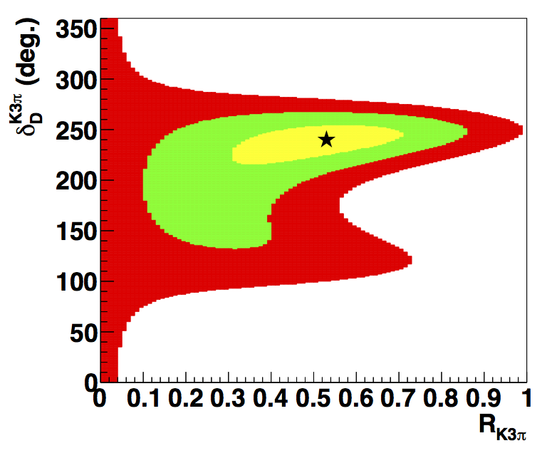
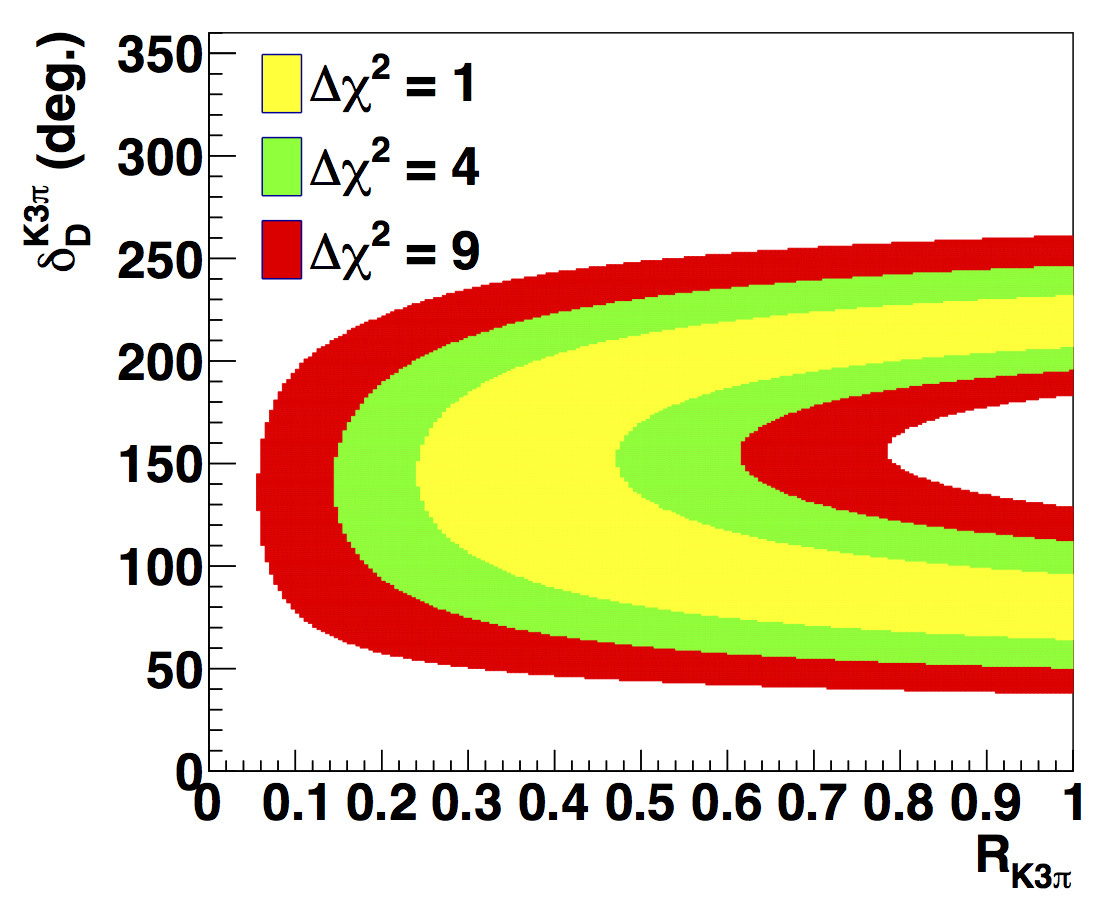
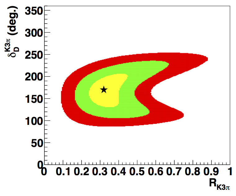
Figure 10: Constraints on $Z^{K3\pi}=R_{K3\pi}e^{-i\delta^{K3\pi}_{D}}$ from (left) CLEO-c Evans et al. (2016), (center) LHCb Aaij et al. (2015h), (right) CLEO-c and LHCb combined Evans et al. (2016).

VI.3 $C\!P$ violation in four body Charm Decays

VI.3.1 Local $C\!P$ violation in four body decays

Comparing $C\!P$-conjugate regions in phase space provides a measure of $C\!P$ violation. Direct $C\!P$ violation results from interference effects between two decay paths that have both a strong and a weak phase difference. In multibody decays, there is a rich interference structure with many different strong phase differences, so one can expect to find locally enhanced $C\!P$ violating effects that would be ‘washed out’ if one integrated over the entire phase space i.e. considered the total decay rates, only. The even richer structure of four-body decays, compared to three-body decays, could lead to further enhanced sensitivity, at the price of a substantially more complex analysis. Comparing the results of amplitude fits for $C\!P$-conjugate decay modes provides a measure of $C\!P$ violation. Such a model-dependent search for direct $C\!P$ violation was performed by CLEO in ${{D}^{0}}\to K^{+}K^{-}\pi^{+}\pi^{-}$ Artuso et al. (2012). Most model-independent searches for local $C\!P$ violation are based on performing a $\chi^{2}$ comparison of the number of events in the bins of $C\!P$–conjugate Dalitz plots. This method was pioneered by BaBar Aubert et al. (2008c) and developed further in Bediaga et al. (2009, 2012), and has been generalised to four-body decays in LHCb’s analysis of ${{D}^{0}}\to{K^{+}}{K^{-}}{\pi^{+}}{\pi^{-}}$ and ${{D}^{0}}\to{\pi^{+}}{\pi^{-}}{\pi^{+}}{\pi^{-}}$ Aaij et al. (2013c). All results have been compatible with $C\!P$ conservation.

VI.3.2 $C\!P$ violation in P-odd observables

While the above examples of $C\!P$ violation searches in four body decays use generalisations of methods used in three-body analyses, there is class of model-independent $C\!P$ violating parameters in four-body decays that is inaccessible to Dalitz plot analyses. These are based on $\hat{T}$ odd observables Golowich and Valencia (1989); Valencia (1989); Bensalem and London (2001); Bigi (2001); Bensalem et al. (2002a, b); Datta and London (2004); Gronau and Rosner (2011); Durieux and Grossman (2015), where $\hat{T}$ represents motion reversal, also referred to as “naïve time reversal” Durieux and Grossman (2015). For the decay of a pseudoscalar to pseudoscalars, $\hat{T}$ is equivalent to parity, so here we refer to them as $P$-odd. As mentioned in Section.VI.1, parity violation is only possible in decays where $N_{f}>3$. In such a case one can define any parity-odd function $w(\mathbf{x})=-w(-\mathbf{x})$, then use this to define the parity sensitive variable,

$$A_{w}=\frac{\int w(\mathbf{x})|\mathcal{A}_{f}(\mathbf{x})|^{2}\left|\frac{\partial{\boldsymbol{\phi}(\mathbf{x})}}{\partial(x_{1},\ldots,x_{n})}\right|\mathrm{d}^{n}x}{\int|w(\mathbf{x})||\mathcal{A}_{f}(\mathbf{x})|^{2}\left|\frac{\partial{\boldsymbol{\phi}(\mathbf{x})}}{\partial(x_{1},\ldots,x_{n})}\right|\mathrm{d}^{n}x},$$ (7)

where a non-zero $A^{f}_{w}$ indicates parity-violation. The same quantity can also be calculated for the $C\!P$ conjugate decay to obtain $\bar{A}^{f}_{w}$. Any difference in parity violation between the two decays i.e. $\mathcal{A}^{C\!P}_{w}={A}_{w}-\bar{A}_{w}\neq 0$ would then indicate $C\!P$ violation. This may just seem like a convoluted method to find $C\!P$-violation, but it is a truly independent observable; usually a prerequisite of $C\!P$-violation is a non-zero strong-phase difference $\delta$ i.e. the magnitude of $C\!P$-violation is proportional to $\sin\delta$. $C\!P$-violation in the observable $\mathcal{A}^{C\!P}_{w}$, however, is proportional to $\cos(\delta_{+}-\delta_{-})$, where $\delta_{+}$ ($\delta_{-}$) is the strong phase associated to a parity-even (parity-odd) part of the amplitude Durieux and Grossman (2015). Such measurements have been made in ${{D}^{0}}\to{K^{+}}{K^{-}}{\pi^{+}}{\pi^{-}}$ and ${D}_{s}^{+}\to K^{+}K_{S}{\pi^{+}}{\pi^{-}}$ using $w(p)=\mathrm{sign}(p_{1}\cdot(p_{2}\times p_{3}))$ Link et al. (2005b); del Amo Sanchez et al. (2010); Lees et al. (2011b); Aaij et al. (2014h). In addition to a phase–space integrated result, LHCb’s analysis Aaij et al. (2014h) is also carried out locally in sub–regions of phase space to enhance the sensitivity of the method. All results so far have been consistent with $C\!P$ conservation.

VI.4 Summary

Four body decays have unique sensitivity to $P$ and $C\!P$ violating variables in charm and beauty decay spectroscopy. The vast, clean samples of such decays available at LHCb and the B-factories, and their upgrades, will lead to new opportunities as well as new challenges. The unprecidented statistical precision will require excellent control of systematic and theoretical uncertainties. Theoretically well-motivated, practically implementable amplitude models for four-body decays matching the superb quality of the data would clearly be highly desirable. At this point, they seem significantly further away than for the three body case.

In the meantime, the focus in controlling theory uncertainties will remain on data-driven, model-independent approaches. Such approaches have been developed, and are continuously being improved, for key measurements like the precision determinations of $\gamma$ or $C\!P$ violation in charm decays. Many of these methods rely on input from the charm threshold. For the measurement of $\gamma$, the precision can be increased further through the use of phase information obtained from charm mixing. However, even model-independent approaches rely on input from amplitude models to optimise their precision. Since these approaches are robust against model-induced biases, even a ‘traditional’ isobar model with Breit Wigner resonances and the much vilified non-resonant term is expected to be very useful. Of course, better descriptions of four body decay amplitudes would be even more valuable.

VI.5 Acknowledgements

We gratefully acknowledge funding from the European Research Council under FP7 / ERC Grant Agreement number 307737.

VII IIB’s View of Theoretical Landscape for LHCb Experimentalists

Ikaros I. Bigi

Department of Physics, University of Notre Dame du Lac
Notre Dame, Indiana, USA

We have to deal with three cultures: Hadrodynamics (HD), HEP & lattice QCD (LQCD). The first one deals with hadrons & their diagrams, while the second & third one with quarks & gluons in different situations. The general challenge is how one can combine them. Obviously I am seen is somewhat ‘biased’, but I think & work in HEP, while I know about the strengths (& weak points) of LQCD. There are sizable differences, as we have seen during the Rio WS. It is not trivial at all to combine them; in my view there is no other option to make progress in understanding underlying dynamics. We are not in a situation where we are looking for a culprit with a smoking gun at the scene of the crime. It is more complex to make the case.

It is usually said that ‘model independent’ analyses are the best information we can get from the data. To say it with different words: the ‘best fitted’ analyses in the future with more data is the final step to understand the underlying dynamics. I agree that is very important. However in my view it is not the final step even with more data. I might been seen as biased as a theorist – however it is crucial to enhance the collaboration between experimenters & theorists on a long time scale. It is crucial to discuss which refined theoretical tools & thinking are best in complex situations; it depends. One has only to look at the history in HEP: the best fits do not always give the best informations.

In this case we cannot just ‘trust’ diagrams; we are in a different era, where we have to go for real precision. My main points:

• ‘Popular’ candidates are (broken) $SU(3)_{Fl}$ and in particular U-spin symmetries. They are fine for spectroscopy, but not, when one includes weak transitions. The difference between U- vs. V-spin symmetries are ‘fuzzy’ for well-know examples like: $D^{0}\to K^{+}K^{-}$ vs. $D^{0}\to\pi^{+}\pi^{-}$ and compare with $D^{0}\to K^{+}K^{-}\pi^{+}\pi^{-}$ vs. $D^{0}\to 2\pi^{+}2\pi^{-}$ etc. etc. It was discussed in some details in Bianco et al. (2003).

  Another example: the lifetimes of $B^{0}$ and $B^{0}_{s}$ are the same within 2%; however we find BR$(B^{0}\to K^{+}\pi^{-})=(1.96\pm 0.05)\cdot 10^{-5}$ vs. BR$(B^{0}_{s}\to K^{+}\pi^{-})=(0.55\pm 0.06)\cdot 10^{-5}$. There are sizable differences between ”inclusive” vs. ”exclusive” ones.

• In general re-scattering/final state interactions Bigi et al. (1988); Wolfenstein (1991); CIC happen all the time in two-body final states (FS), but even more crucial for many-body FS. For the future we have to work on the connection of the ‘cultures’ of HD and HEP. Here I use the language of quarks: $\bar{q}_{i}q_{i}\to\bar{q}_{j}q_{j}+\bar{q}_{k}q_{k}\bar{q}_{l}q_{l}+...$; it crucially depends on strong forces. However, it does not mean that it is under quantitative control of our understanding of QCD – unless we get ”help” with other tools.

• The impacts of penguin diagrams were first shown about $\Delta I=3/2$ $\ll$ $\Delta I=1/2$ in kaon decays and direct CPV in $\epsilon^{\prime}/\epsilon_{K}\neq 0$. They are based on local operators. The expected SM predictions are effected by large uncertainties. We have also sizable experimental uncertainties: ${\rm Re}(\epsilon^{\prime}/\epsilon_{K})_{\rm exp.}=(1.66\pm 0.23)\cdot 10^{-3}$. We have the first result from the LQCD culture Garron (2015): ${\rm Re}(\epsilon^{\prime}/\epsilon_{K})_{\rm LQCD}=(0.138\pm 0.515\pm 0.443)\cdot 10^{-3}$. Obviously our community needs more lattice ‘data’ & more analyses. Of course the LHCb collaboration will not go after these transitions; my point is: when somebody goes after accuracy or even precision, one has be careful to use just diagrams.

  We can discuss the impact of penguin diagrams on inclusive lifetimes of beauty (& charm) hadrons and in CKM suppressed decays of $B_{(s)}$ for $b\to q$ with $q=s,d$. Their impact is described with short distance QCD like for $\Delta\Gamma(B_{q})$.

  We know about the impact of penguins in those items in at least semi-quantitatively. However the situations are much more ‘complex’ for exclusive decays of heavy flavor hadrons. Penguin diagrams might show us the ‘road’, but we need much more thinking, working and apply other tools like chiral symmetry, dispersion relations etc.; it needs time.

Now I talk specifically for beauty and charm hadrons:

• We know that the SM produces at least the leading source of CPV. Therefore the goal is to establish New Dynamics (ND) and maybe even its features. It is crucial to measure ”regional” CP asymmetries in $B\to K\pi\pi$ vs. $B\to 3K$ and $B\to 3\pi$ vs. $B\to\pi 2K$ with more accuracies. We have learnt that ”regional” CP asymmetries are large. The definition of ”regional” asymmetries is important; furthermore it depends on the differences between narrow resonances vs. broad ones vs. non-resonances. Even CPT invariance seems to be ‘usable’.

• We cannot stop at three-body FS; we have to go to four-body FS and probe semi-regional asymmetries.

• We have to probe CPV in the CKM suppressed decays of $\Lambda_{b}$. I think we can deal with production asymmetries in $pp$ collisions. Finally it seems that even Belle II will not compete there.

• Obviously we have to probe CPV both in SCS and DCS in the decays of charm mesons & baryons. The SM gives basically zero CPV in DCS ones. Most decays of those give mostly three- and four-body FS.

  Again it is important to probe regional asymmetries; we have to go beyond moments with four-body FS and compare $D\to 4\pi$ vs. $D\to\bar{K}K2\pi$.

• However, there is a question: how do you ”define regional” asymmetries. In particular it needs some ”intelligent” judgment about four-body FS; probing phase spaces is not. Furthermore re-scattering connects $4\pi$ FS with $\bar{K}K2\pi$ one. In general we have to compare $D^{0}$, $D^{+}$ & $D^{+}_{s}$ transitions.

  Finally in the future we have to probe DCS decays like: $D^{+}\to K^{+}\pi^{+}\pi^{-}/K^{+}K^{+}K^{0}$, $D^{0}\to K^{+}\pi^{+}\pi^{-}\pi^{-}/K^{+}K^{+}K^{-}\pi^{-}$ and $D_{s}^{+}\to K^{+}K^{+}\pi^{-}$.

• We have to probe CPV in the decays of $\Lambda_{c}^{+}$ at least.

• Dynamics close to thresholds are very complex. Probing CP asymmetries give us much more information, where it comes from resonances or not, shows our limit so far about understanding strong forces - or the impact of New Dynamics Pennington (2002); *DR_b; *DR_c; Hanhart (2013); *KUBIS_b; *KUBIS_c.

My main points are: we have to go beyond diagrams & U-spin symmetry; they are connected with V-spin symmetry based on CPT invariance. We have to probe CP asymmetries in baryons, non-leading sources of CPV for beauty transitions & in general for charm ones and the impact of ND & its features. Again, it is crucial to combine two cultures in fundamental dynamics. Correlation, correlations, correlations!

In the real world there is a good reason to give short contributions in Proceedings. I explain my points in detail in Bigi (2015a, b).

Acknowledgments: This work was supported by the NSF under the grant numbers PHY-1215979 & PHY-1520966.

VIII Parametrization of three-body hadronic $D$ decay amplitudes

Diogo Boito^a,b and Benoît Loiseau^c

^aInstituto de Física de São Carlos, Universidade de São Paulo,
CP 369, 13560-970, São Carlos, SP, Brazil
^bInstituto de Física, Universidade de São Paulo,
São Paulo, SP, Brazil
^cSorbonne Universités, Pierre & Marie Curie et Paris Diderot, IN2P3-CNRS,
Laboratoire de Physique Nucléaire et de Hautes Energies, Groupe Phenomenologie, 4 place Jussieu, 75252 Paris, France

In order to constrain the Dalitz-plot analyses of hadronic three-body $D$ decays we suggest here parametrizations of $D^{+}\to K^{-}\pi^{+}\pi^{+}$ and $D^{0}\to K^{0}_{S}\pi^{-}\pi^{+}$ amplitudes that can be readily implemented in experimental analyses. Our parametrizations are derived in the quasi-two-body factorization approach where the two-body final state interactions are fully taken into account by unitary hadronic form factors. In particular, we tackle here the cases of the $S$- and $P$-wave $K^{-}\pi^{+}$ pairs in $D^{+}\to K^{-}\pi^{+}\pi^{+}$ and $K^{0}_{S}\pi^{-}$ in $D^{0}\to K^{0}_{S}\pi^{-}\pi^{+}$, where the scalar and vector $K\pi$ form factors play a decisive role. Parametrizations of other three-body hadronic $D$ and $B$ decay amplitudes are in progress and will be presented elsewhere.

VIII.1 Introduction: quasi two-body factorization approach

The two-body QCD factorization, as a leading order approximation in an expansion in $\alpha_{s}$ and inverse powers of the $b$ quark mass, has been applied with success to charmless nonleptonic $B$ decays (see e.g. Ref. Beneke and Neubert (2003)). The charm quark mass, $m_{c}\sim 1.2$ GeV, is smaller than the bottom quark mass which enhances corrections to the factorized results. Factorization for $D$ decays is less predictive inasmuch as it does not allow for systematic improvement. Nevertheless, as a phenomenological approach, since the initial articles of Bauer, Stech and Wirbel Bauer et al. (1987), the factorization hypothesis has been applied successfully to $D$ decays, provided one treats Wilson coefficients as phenomenological parameters to account for possibly important non-factorizable corrections Biswas et al. (2015).

So far there is no factorization scheme for three-body decays. However, three-body decays of $D$ and $B$ mesons have important contributions from intermediate resonances — such as those of the $\rho(770)$ and $K^{*}(892)$ — and can therefore be considered as quasi two-body decays. One assumes that two of the three final-state mesons form a single state originating from a quark-antiquark pair, which leads to quasi two-body final states so that the factorization procedure can be applied. Then, the three-body final state is reconstructed with the use of two-body mesonic form factors to account for the important hadronic final state interactions. For instance, for the $D^{0}\to K^{0}_{S}\pi^{-}\pi^{+}$ decays, the three-meson final state $K^{0}_{S}\pi^{+}\pi^{-}$ is supposed to be formed by the quasi two-body pairs, $[K^{0}_{S}\pi^{+}]_{L}\ \pi^{-}$, $[K^{0}_{S}\pi^{-}]_{L}\ \pi^{+}$ and $K^{0}_{S}\ [\pi^{+}{\pi^{-}}]_{L}$, where two of the three mesons form a state in $L=S,P$ or $D$ wave. This framework has been successfully employed to several three-body $B$ and $D$ decays Boito et al. (2009); Boito and Escribano (2009); Dedonder et al. (2014); El-Bennich et al. (2009).

As a concrete example of this procedure let us apply it to the $D^{+}\to K^{-}\pi^{+}\pi^{+}$ case. The amplitude given by $\langle K^{-}\pi^{+}\pi^{+}|{\cal H}_{\rm eff}|D^{+}\rangle$ receives contributions from two topologies and factorizes as

$${\cal A}(D^{+}\to K^{-}\pi^{+}\pi^{+})=\frac{G_{F}}{\sqrt{2}}\cos^{2}\theta_{C}[a_{1}\langle K^{-}\pi^{+}_{1}|\bar{s}\gamma^{\mu}(1-\gamma_{5})c|D^{+}\rangle\langle\pi^{+}_{2}|\bar{u}\gamma_{\mu}(1-\gamma_{5})d|0\rangle$$

$$+a_{2}\langle K^{-}\pi^{+}_{1}|\bar{s}\gamma^{\mu}(1-\gamma_{5})d|0\rangle\langle\pi^{+}_{2}|\bar{u}\gamma_{\mu}(1-\gamma_{5})c|D^{+}\rangle]+(\pi_{1}^{+}\leftrightarrow\pi_{2}^{+}).$$ (8)

In the above expression $G_{F}$ is the Fermi constant, $\theta_{C}$ the Cabbibo angle and $a_{1,2}$ Buras (1995) are combinations of Wilson coefficients of the effective weak Hamiltonian. In the expression factorized as above, the $K\pi$ form factors appear explicitly in the matrix element $\langle K^{-}\pi^{+}_{1}|\bar{s}\gamma^{\mu}(1-\gamma_{5})d|0\rangle$. The evaluation of $\langle K^{-}\pi^{+}_{1}|\bar{s}\gamma^{\mu}(1-\gamma_{5})c|D^{+}\rangle$ is less straightforward. However, assuming this transition to proceed through the dominant intermediate resonances, this matrix element can also be written in terms of the $K\pi$ form factors Gardner and Meissner (2002b). The other matrix elements of Eq. (VIII.1) can be written in terms of decay constants or transitions form factors that can be extracted from semi-leptonic decays.

In the next section we cast the amplitudes for the decays $D^{+}\to[K^{-}\pi^{+}]_{S,P}\ \pi^{+}$ and $D^{0}\to[K^{0}_{S}\pi^{-}]_{S,P,D}\ \pi^{+}$ in forms that can be readily used in data analyses.

VIII.2 Examples of amplitude parametrizations

Parametrization of the $D^{+}\to[K^{-}\pi^{+}]_{S,P}\ \pi^{+}$ amplitudes

We use the following notation for the invariant masses of the final state $s_{1}=(p_{K^{-}}+p_{\pi^{+}_{1}})^{2}$, $s_{2}=(p_{K^{-}}+p_{\pi^{+}_{2}})^{2}$ and $s_{12}=(p_{\pi^{+}_{1}}+p_{\pi^{+}_{2}})^{2}$. From the results of Ref. Boito and Escribano (2009), obtained within the quasi two-body factorization approach, one can parametrize the $S$- and $P$-wave amplitudes for $D^{+}\to[K^{-}\pi^{+}]_{S,P}\ \pi^{+}$ as

$$\mathcal{A}^{D^{+}}_{S}(s_{1},s_{2},s_{12}) =\left[c_{0}^{S}(m_{D}^{2}-s_{1})+c_{1}^{S}\frac{F_{0}^{D\pi}(s_{1})}{s_{1}}\right]F_{0}^{K\pi}(s_{1}),$$

$$\mathcal{A}^{D^{+}}_{P}(s_{1},s_{2},s_{12}) =\left[c_{0}^{P}\Omega(s_{1},s_{2},s_{12})+c_{1}^{P}\left(\frac{s_{2}-s_{12}}{\Delta^{2}}-\frac{1}{s_{1}}\right)F_{1}^{D\pi}(s_{1})\right]F_{1}^{K\pi}(s_{1}),$$ (9)

with $\Omega(s_{1},s_{2},s_{12})=s_{2}-s_{12}-\Delta^{2}/s_{1}$ and $\Delta^{2}=(m_{K}^{2}-m_{\pi}^{2})(m^{2}_{D}-m^{2}_{\pi})$. In Eq. (VIII.2), $c_{0,1}^{S,P}$ are free complex parameters to be fitted. We have assumed that the Wilson coefficients of the effective weak Hamiltonian get wave dependent non-factorizable corrections. The $S$- plus $P$-wave amplitude has then 7 (real) free parameters, since one global phase cannot be observed. They can be related to those of Ref. Boito and Escribano (2009) through a comparison with Eqs. (3), (8) and (35) of that work. If we drop the assumption that the corrections to Wilson coefficients depend on the angular momentum of the $K\pi$ pair, the number of free parameters is reduced to 4. In Eq. (VIII.2) $F_{0,1}^{D\pi}(s_{1})$ are the scalar and vector $D$ to $\pi$ transition form factors and $F_{0,1}^{K\pi}(s_{1})$ the scalar and vector $K\pi$ form factors.

A parametrization of the type of Eq. (VIII.2) has been introduced $S$- and $P$-wave $K\pi$ pairs. The parameters in that work were obtained from integrated branching ratios, and not from a Dalitz plot analysis. Nevertheless, the results were satisfactory for $\sqrt{s_{1,2}}\lesssim$1.55 GeV. Additional contributions, e.g. with higher angular momentum or the isospin-2 $\pi^{+}\pi^{+}$ interactions, are very small in this process. In a realistic Dalitz plot analysis, however, they may be required and have to be included in the signal function through usual isobar model expressions, for example.

Parametrization of the $D^{0}\to[K^{0}_{S}\pi^{-}]_{S,P,D}\ \pi^{+}$ amplitudes

In an amplitude analysis, using quasi-two body factorization, Ref. Dedonder et al. (2014) has obtained good fits to the Belle Dalitz plot density distribution and to that of a BABAR model for the $D^{0}\to K^{0}_{S}\pi^{-}\pi^{+}$ decays. The following parametrization, for the $D^{0}\to[K^{0}_{S}\pi^{-}]_{S,P,D}\ \pi^{+}$ amplitudes, is based on the amplitudes derived from Eqs. (66) and (68) in Ref. Dedonder et al. (2014). One has, with $s_{-}=(p_{K^{0}_{S}}+p_{\pi^{-}})^{2}$, $s_{+}=(p_{K^{0}_{S}}+p_{\pi^{+}})^{2}$ and $s_{0}=(p_{\pi^{-}}+p_{\pi^{+}})^{2}$,

$$\mathcal{A}^{D^{0}}_{S}(s_{0},s_{-},s_{+}) = \left(d_{0}^{S}+d_{1}^{S}s_{-}\right)F_{0}^{K\pi}(s_{-}),$$

$$\mathcal{A}^{D^{0}}_{P}(s_{0},s_{-},s_{+}) = \left(s_{0}-s_{+}+\frac{\Delta^{2}}{s_{-}}\right)d_{0}^{P}F_{1}^{K\pi}(s_{-}).$$ (10)

Here the $S$- plus $P$-wave amplitude $\mathcal{M}^{D^{0}}(s_{0},s_{-},s_{+})=\mathcal{A}^{D^{0}}_{S}(s_{0},s_{-},s_{+})+\mathcal{A}^{D^{0}}_{P}(s_{0},s_{-},s_{+})$ depends on 3 free complex parameters, $d_{0,1}^{S}$ and $d_{0}^{P}$ which can also be related to the parameters appearing in the Eqs. (66) and (68) of Ref. Dedonder et al. (2014).

Despite its small fit fraction, the $D^{0}\to[K^{0}_{S}\pi^{-}]_{D}\ \pi^{+}$ amplitude can play an important role through interference and from Eq. (76) of Ref. Dedonder et al. (2014), it can be parametrized as

$$\mathcal{A}^{D^{0}}_{D}(s_{0},s_{-},s_{+})=\left(d_{0}^{D}+d_{1}^{D}s_{-}\right)B_{K^{*}_{2}}(s_{+},s_{-}),$$ (11)

where the contribution of the $K^{*-}_{2}(1430)$ resonance is described by the relativistic Breit-Wigner function $B_{K^{*}_{2}}(s_{+},s_{-})$ whose expression is given by Eq. (73) of Ref. Dedonder et al. (2014). Here again the two complex parameters $d_{0,1}^{D}$ are related to those entering Eqs. (76) to (78) of Ref. Dedonder et al. (2014).

Finally, there will be analogous parametrizations for the $D^{0}\to[K^{0}_{S}\pi^{+}]_{S,P,D}\ \pi^{-}$ amplitudes and the contribution from the $\pi^{+}\pi^{-}$ final state interactions can also be parametrized in a similar way by introducing $\pi\pi$ form factors Dedonder et al. (2014).

Relative phase

It is important to emphasize that in the total amplitude for the decay rates one cannot have access to a global phase. Therefore, one of the global phases of the partial wave amplitudes can be set to zero. This reduces the number of free (real) parameters in Eqs. (VIII.2) and (VIII.2) by one. Experimental groups often take the $P$-wave, dominated by the $\rho(770)$ or $K^{*}(892)$, as the reference wave and hence impose, by convention, the $P$-wave phase to be zero. This global phase difference between the $S$- and $P$-waves plays an important role in generating the correct pattern of interferences observed in the Dalitz plot analyses. In the parametrization outlined here this phase difference is obtained empirically from data.

Form factors

In Eqs. (VIII.2) and (VIII.2), the $K\pi$ form factors play a crucial role. Those employed in our works are obtained from dispersion relations accounting for analyticity and unitarity constraints El-Bennich et al. (2009); Jamin et al. (2006); Moussallam (2008); Boito et al. (2010). The scalar form factor includes the contribution of the $K^{*}_{0}(800)$ and $K^{*}_{0}(1430)$ and the vector form factor those of $K^{*}(892)$ and $K^{*}(1410)$. The non-resonant background is automatically included. The scalar and vector $D$ to $\pi$ transition form factors can be parametrized following Ref. Melikhov (2002) (see, e.g., Eqs. (116) and (117) of Ref. Dedonder et al. (2014)).

VIII.3 Concluding remarks and outlook

In this note we suggest the replacement of the sums of Breit-Wigner expressions, often used in Dalitz plot analyses, by amplitudes parametrized in terms of unitary form factors. Those are determined by coupled channel equations based on experimental meson-meson $T$-matrix elements together with chiral symmetry and asymptotic QCD constraints. Our amplitudes also carry information about the weak vertex, described within the quasi-two body factorization approach. In collaboration with J. P. Dedonder, B. El-Bennich, R. Escribano, R. Kamiński, L. Leśniak, we are working on parametrizations for other three-body hadronic $D$ and $B$ decays, that will be presented elsewhere. We will, upon request, provide C++ functions ready for use, e.g., in CERN/Root.

Acknowledgements It is a pleasure to thank Alberto dos Reis and the organizers of the workshop as well as the Centro Brasileiro de Pesquisas Físicas (CBPF) for hosting this fruitful meeting. Jean-Pierre Dedonder and Bruno El-Bennich must be thanked for very helpful discussions. The work of DB was supported by the São Paulo Research Foundation (FAPESP) grant 2014/50683-0. BL’s work received support from FAPESP (grant 2015/04772-6) and from LFTC, UNICSUL.

IX Testing the SM with 3-body $B$ Decays

Bhubanjyoti Bhattacharya and David London

Physique des Particules, Université de Montréal,
C.P. 6128, succ. centre-ville, Montréal, QC, Canada H3C 3J7

Abstract
An amplitude analysis can be used to extract the amplitudes of charmless $B\to PPP$ decays from their Dalitz plots. Here we describe two methods that use such an amplitude analysis to perform clean tests of the standard model (SM). Both methods use flavor SU(3) symmetry. We argue that SU(3)-breaking effects, which could be responsible for discrepancies with the SM predictions, may be reduced by averaging over the Dalitz plot. We show how this conjecture can be tested experimentally. We also address some questions, related to rescattering, that arose at the LHCb workshop.

IX.1 Introduction

One of the main purposes of the LHCb workshop on multi-body decays of $B$ and $D$ mesons was to re-examine the analysis used to reconstruct the amplitudes of 3-body $B$ decays from their Dalitz plots. Here we describe two methods that use such an amplitude analysis to perform clean tests of the standard model (SM).

Under flavor SU(3) symmetry, there are three identical final-state particles in charmless $B\to PPP$ decays, so that the six permutations of these particles must be taken into account. This leads to six final-state symmetries: there are one totally symmetric, one totally antisymmetric, two mixed-symmetric, and two mixed-antisymmetric states. In $B\to P_{1}P_{2}P_{3}$ decays, the relative angular momenta of the $P_{i}$ are not fixed, so all six symmetry states are possible. The physical $P_{1}P_{2}P_{3}$ state is a linear combination of all six states.

The symmetry states can be isolated with an amplitude analysis. The $B\to P_{1}P_{2}P_{3}$ amplitude is written as

$${\cal M}(s_{12},s_{13})={\cal N}_{\rm DP}\sum\limits_{j}c_{j}e^{i\theta_{j}}F_{j}(s_{12},s_{13})\leavevmode\nobreak\ .$$ (12)

The form of the $F_{j}$ depends on the particular contribution to the amplitude (resonant or non-resonant), and the $c_{j}$ and $\theta_{j}$ can be extracted from a fit to the Dalitz-plot event distribution. Given these quantities, ${\cal M}(s_{12},s_{13})$ can be reconstructed. The amplitude for a state with a given symmetry is then found by applying this symmetry to ${\cal M}(s_{12},s_{13})$. For example, the fully-symmetric (FS) final-state amplitude is

$${\cal M}_{\rm FS} = \frac{1}{\sqrt{6}}\left[{\cal M}(s_{12},s_{13})+{\cal M}(s_{13},s_{12})+{\cal M}(s_{12},s_{23})\right.$$ (13)

$$\hskip 42.67912pt\left.+\leavevmode\nobreak\ {\cal M}(s_{23},s_{12})+{\cal M}(s_{23},s_{13})+{\cal M}(s_{13},s_{23})\right]\leavevmode\nobreak\ .$$

The FS state is particularly interesting because it receives no contributions from spin-1 resonances. Furthermore, the FS state can be used to test the SM. Methods are described in the following two sections.

IX.2 Amplitude Equalities

It was shown in Ref. Bhattacharya et al. (2014a) that two amplitude equalities follow from U-spin transformations. They are

$$\sqrt{2}{\cal A}(B^{+}\to K^{+}\pi^{+}\pi^{-})_{\rm FS} = {\cal A}(B^{+}\to K^{+}K^{+}K^{-})_{\rm FS}\leavevmode\nobreak\ ,$$

$$\sqrt{2}{\cal A}(B^{+}\to\pi^{+}K^{+}K^{-})_{\rm FS} = {\cal A}(B^{+}\to\pi^{+}\pi^{+}\pi^{-})_{\rm FS}\leavevmode\nobreak\ ,$$ (14)

which we refer to as the $K\pi\pi$-$KK{\bar{K}}$ and $\pi K{\bar{K}}$-$\pi\pi\pi$ relations, respectively. These relations can be probed experimentally, providing clean tests of the SM.

Question: Flavor SU(3) (or U spin) is only an approximate symmetry. Can it really be used in tests of the SM? Answer: Absolutely, but SU(3) breaking must be kept in mind. In particular, if either of the above amplitude equalities is found not to hold, it could simply be due to SU(3)-breaking effects. In all of these tests, the possibility of SU(3) breaking must be addressed.

Question: Could rescattering break the amplitude equalities? Answer: Only if it includes an SU(3)-breaking effect. Rescattering that respects SU(3) is included in the amplitude equalities.

Consider the $K\pi\pi$-$KK{\bar{K}}$ relation. It can be written as

$$\frac{|{\cal A}(B^{+}\to K^{+}K^{+}K^{-})_{\rm FS}|}{\sqrt{2}|{\cal A}(B^{+}\to K^{+}\pi^{+}\pi^{-})_{\rm FS}|}=1\leavevmode\nobreak\ .$$ (15)

(This also holds for $B^{-}$ decays.) The $K\pi\pi$-$KK{\bar{K}}$ relation is momentum dependent, and holds at every point in the Dalitz plot. Thus, the above ratio should be measured for each Dalitz-plot point, and then one should average over all points. This will reduce the statistical error. Also: recall that the FS amplitudes are reconstructed from a fit to the full Dalitz plot. The errors on the ratio at different points are therefore correlated. These correlations must be taken into account in calculating the total error resulting from averaging.

A similar analysis can be done for the $\pi K{\bar{K}}$-$\pi\pi\pi$ relation.

IX.2.1 SU(3) breaking

What about SU(3) breaking? In the presence of SU(3) breaking, we have

$$\frac{|{\cal A}(B^{+}\to K^{+}K^{+}K^{-})_{\rm FS}|}{\sqrt{2}|{\cal A}(B^{+}\to K^{+}\pi^{+}\pi^{-})_{\rm FS}|}=|X|\leavevmode\nobreak\ ,$$ (16)

where $X$ is the SU(3)-breaking factor. It is a complex number that depends in a complicated way on all the group-theoretical SU(3)-breaking terms, and can take different values at different points in the Dalitz plot. Its size is unknown, though, based on SU(3)-breaking effects in two-body decays, one might naively estimate its deviation from 1 to be $O(30\%)$. Now, it seems reasonable to expect that $|X|-1>0$ at some points of the Dalitz plot, and $|X|-1<0$ at others. In this situation, averaging over all Dalitz-plot points will reduce the effect of SU(3) breaking. If so, the deviation of $X$ from 1 will be found to be much smaller than $O(30\%)$.

Of course, there is no guarantee that this occurs for the $K\pi\pi$-$KK{\bar{K}}$ relation (and SU(3) breaking could be smaller simply due to the fact that all spin-1 resonances, and the associated SU(3) breaking, are absent from the FS amplitudes). However, the key point is that one can experimentally test whether the theoretical error is indeed reduced when one averages over the Dalitz plot.

Now consider a pair of $B$ decays – one ${\bar{b}}\to{\bar{d}}$, the other ${\bar{b}}\to{\bar{s}}$ – that are related by U-spin reflection ($d\leftrightarrow s$). It has been shown Gronau (2000) that, in the U-spin limit, the four observables $B_{d,s}$ (branching ratios) and $A^{CP}_{d,s}$ (direct CP asymmetries) are not independent, but obey

$$-\frac{A^{CP}_{s}}{A^{CP}_{d}}\,\frac{\tau(B^{0})B_{s}}{\tau(B_{s}^{0})B_{d}}=1\leavevmode\nobreak\ .$$ (17)

One 3-body decay pair to which this relation applies is $B^{+}\to\pi^{+}K^{+}K^{-}$ and $B^{+}\to K^{+}\pi^{+}\pi^{-}$. The relation holds at each point on the Dalitz plot.

But what about U-spin breaking? Using the same logic as above, we expect that any U-spin breaking is reduced when one averages over all Dalitz-plot points. That is, we write

$$-\frac{A^{CP}_{s}}{A^{CP}_{d}}\,\frac{\tau(B^{0})B_{s}}{\tau(B_{s}^{0})B_{d}}=N\leavevmode\nobreak\ .$$ (18)

In the U-spin limit, $N=1$. By measuring $B_{d,s}$ and $A^{CP}_{d,s}$, and constructing the above ratio, it is possible to experimentally determine if an average over all Dalitz-plot points leads to $N\to 1$. If so, this supports the conjecture that SU(3)-breaking effects are also reduced by averaging. (Note that no amplitude analysis is required for this test.)

IX.3 Extraction of $\gamma$ using an amplitude analysis

In this section we describe the method for extracting $\gamma$ from $B\to PPP$ decays using an amplitude analysis Rey-Le Lorier and London (2012); Bhattacharya et al. (2014b).

It was shown in Ref. Lorier et al. (2011) that the amplitudes for each $B\to PPP$ symmetry state can be expressed in terms of diagrams. These are similar to those of two-body $B$ decays ($T$, $C$, etc.), except that (i) they are momentum dependent, and (ii) for $B\to PPP$ decays one has to “pop” a quark pair from the vacuum. Diagrams have the subscript “1” (“2”) if the popped quark pair is between two non-spectator final-state quarks (two final-state quarks including the spectator).

Question: Doesn’t rescattering ruin the diagrammatic description of amplitudes? For example, what do penguin diagrams even mean in the presence of rescattering? Answer: There was a great deal of confusion at the workshop about diagrams and rescattering. Indeed, the simple use of penguin diagrams was called into question. However, this is all a red herring. The diagrams include rescattering. For example, consider the decay $B^{+}\to\pi^{+}K^{0}$, which is ${\bar{b}}\to{\bar{s}}d{\bar{d}}$ at the quark level. One of the diagrams contributing to this decay is a gluonic penguin: ${\bar{b}}\to{\bar{s}}g^{*}(\to d{\bar{d}})$. Now, one of the gluonic penguin diagrams has an internal $c$ quark, and is proportional to $V_{cb}^{*}V_{cs}$. It represents the tree-level decay ${\bar{b}}\to{\bar{c}}c{\bar{s}}$, with the $c{\bar{c}}$ pair rescattering to $d{\bar{d}}$. If the momentum transfer is large, this is short-distance scattering, and can be thought of as $c{\bar{c}}\to d{\bar{d}}$ via the exchange of a single gluon. However, if the momentum transfer is small, this becomes a long-distance effect involving multiple gluon exchange, or taking place at the hadronic level. Regardless, this penguin diagram includes such rescattering processes as $B^{+}\to D_{s}^{+}{\bar{D}}^{0}\to\pi^{+}K^{0}$. The point is that the diagrammatic decomposition of a decay amplitude takes rescattering into account, and this holds for $B\to PPP$ decays.

Now consider the five decays $B^{0}\to K^{+}\pi^{0}\pi^{-}$, $B^{0}\to K^{0}\pi^{+}\pi^{-}$, $B^{+}\to K^{+}\pi^{+}\pi^{-}$, $B^{0}\to K^{+}K^{0}K^{-}$, and $B^{0}\to K^{0}K^{0}{\bar{K}}^{0}$. The $B\to K\pi\pi$ diagrams involve a popped $u{\bar{u}}$ or $d{\bar{d}}$ quark pair, while those of $B\to KK{\bar{K}}$ have a popped $s{\bar{s}}$ pair. But flavor SU(3) symmetry makes no distinction between $u{\bar{u}}$, $d{\bar{d}}$ or $s{\bar{s}}$, so that the five amplitudes are written in terms of the same diagrams.

The decay amplitudes for the FS states are given by

$$2A(B^{0}\to K^{+}\pi^{0}\pi^{-})_{\rm FS} = be^{i\gamma}-\kappa c\leavevmode\nobreak\ ,$$

$$\sqrt{2}A(B^{0}\to K^{0}\pi^{+}\pi^{-})_{\rm FS} = -de^{i\gamma}-{\tilde{P}}^{\prime}_{uc}e^{i\gamma}-a+\kappa d\leavevmode\nobreak\ ,$$

$$\sqrt{2}A(B^{+}\to K^{+}\pi^{+}\pi^{-})_{\rm FS} = -ce^{i\gamma}-{\tilde{P}}^{\prime}_{uc}e^{i\gamma}-a+\kappa b\leavevmode\nobreak\ ,$$

$$\sqrt{2}A(B^{0}\to K^{+}K^{0}K^{-})_{\rm FS} = \alpha_{SU(3)}(-ce^{i\gamma}-{\tilde{P}}^{\prime}_{uc}e^{i\gamma}-a+\kappa b)\leavevmode\nobreak\ ,$$

$$A(B^{0}\to K^{0}K^{0}{\bar{K}}^{0})_{\rm FS} = \alpha_{SU(3)}({\tilde{P}}^{\prime}_{uc}e^{i\gamma}+a)\leavevmode\nobreak\ ,$$ (19)

where ${\tilde{P}}^{\prime}_{uc}$ is a penguin diagram, $a$-$d$ are linear combinations of diagrams (see Ref. Bhattacharya et al. (2014b)), and

$$\kappa\equiv-\frac{3}{2}\frac{|V^{*}_{tb}V_{ts}|}{|V^{*}_{ub}V_{us}|}\frac{c_{9}+c_{10}}{c_{1}+c_{2}}\leavevmode\nobreak\ .$$ (20)

There are many possible SU(3)-breaking effects between the $B\to K\pi\pi$ and $B\to KK{\bar{K}}$ diagrams, but they cannot all be included in a fit. Instead, we assume that there is only a single SU(3)-breaking parameter, $\alpha_{SU(3)}$.

As written above, the five FS amplitudes depend on 11 theoretical parameters: the magnitudes of ${\tilde{P}}^{\prime}_{uc}$ and $a$-$d$ (5), their relative strong phases (4), $\gamma$, and $|\alpha_{SU(3)}|$. But there are 13 experimental observables: the decay rates and direct CP asymmetries of each of the five processes, and the indirect CP asymmetries of $B^{0}\to K^{0}\pi^{+}\pi^{-}$, $B^{0}\to K^{+}K^{0}K^{-}$ and $B^{0}\to K^{0}K^{0}{\bar{K}}^{0}$. With more observables than theoretical parameters, $\gamma$ can be extracted from a fit, even with the inclusion of $|\alpha_{SU(3)}|$ as a fit parameter.

In addition, since the SU(3)-breaking effects are momentum dependent, their effect on $\gamma$ will vary from point to point on the Dalitz plot. Thus, as before, we expect that averaging over all Dalitz-plot points will reduce the effect of SU(3) breaking, so that the extracted value of $\gamma$ will be close to its true value. This also holds for $\alpha_{SU(3)}$ alone.

In order to perform the fit, one must first extract the FS amplitudes ${\cal M}_{\rm FS}$ and ${\overline{\cal M}}_{\rm FS}$ for each of the five processes and their CP conjugates using an amplitude analysis of their Dalitz plots. Then, using these FS amplitudes, one generates the observables for each decay. The effective CP-averaged branching ratio ($X$), direct CP asymmetry ($Y$), and indirect CP asymmetry ($Z$) are obtained at each Dalitz-plot point as follows:

$$X(s_{12},s_{13}) = |{\cal M}_{\rm FS}(s_{12},s_{13})|^{2}+|\overline{{\cal M}}_{\rm FS}(s_{12},s_{13})|^{2}\leavevmode\nobreak\ ,$$

$$Y(s_{12},s_{13}) = |{\cal M}_{\rm FS}(s_{12},s_{13})|^{2}-|\overline{{\cal M}}_{\rm FS}(s_{12},s_{13})|^{2}\leavevmode\nobreak\ ,$$

$$Z(s_{12},s_{13}) = {\rm Im}\left[{\cal M}^{*}_{\rm FS}(s_{12},s_{13})\leavevmode\nobreak\ \overline{{\cal M}}_{\rm FS}(s_{12},s_{13})\right]\leavevmode\nobreak\ .$$ (21)

Given the theoretical expressions for the FS amplitudes [Eq. (IX.3)], we know how $X$, $Y$ and $Z$ depend on the theoretical unknowns. And given the values of these observables, one can perform a fit at each Dalitz-plot point. Of all the theoretical parameters, only $\gamma$ is the same at each point (i.e., it is momentum-independent). One can therefore combine the results of all the fits to extract the preferred value of $\gamma$. Note that the errors on $X$, $Y$ and $Z$ at different points are correlated. These correlations must be taken into account in calculating the total error on $\gamma$.

In fact, BaBar has measured the Dalitz plots for each of the five decays of interest. In Ref. Bhattacharya et al. (2014b), we performed a preliminary fit using this data and found the following intriguing result. There are four preferred values for $\gamma$:

$$(31^{+2}_{-3})^{\circ}\leavevmode\nobreak\ \leavevmode\nobreak\ ,\leavevmode\nobreak\ \leavevmode\nobreak\ \leavevmode\nobreak\ \leavevmode\nobreak\ (77\pm 3)^{\circ}\leavevmode\nobreak\ \leavevmode\nobreak\ ,\leavevmode\nobreak\ \leavevmode\nobreak\ \leavevmode\nobreak\ \leavevmode\nobreak\ (258^{+4}_{-3})^{\circ}\leavevmode\nobreak\ \leavevmode\nobreak\ ,\leavevmode\nobreak\ \leavevmode\nobreak\ \leavevmode\nobreak\ \leavevmode\nobreak\ (315^{+3}_{-2})^{\circ}\leavevmode\nobreak\ .$$ (22)

Three of these indicate new physics (is this a “$K\pi\pi$-$KK{\bar{K}}$ puzzle”?). But one solution – $(77\pm 3)^{\circ}$ – is consistent with the standard model.

Furthermore, we found that, when averaged over the points, $|\alpha_{SU(3)}|=0.97\pm 0.05$ is found, i.e., this SU(3) breaking is small. This supports the conjecture that the full SU(3) breaking is small when averaged over the Dalitz plot. Of course, as noted above, the full effect of SU(3) breaking is not simply encoded in $\alpha_{SU(3)}$. However, an estimate of this theoretical error can be obtained from the experimental measurements of SU(3) breaking in Eqs. (16) and (18).

IX.4 Conclusions

An amplitude analysis of charmless $B\to PPP$ decays can be used to construct the fully-symmetric (FS) amplitude of the $PPP$ final state. We have described two methods that use the FS amplitudes of 3-body $B$ decays to perform clean tests of the SM. One of these uses the fact that, within flavor SU(3), the SM predicts $\sqrt{2}{\cal A}(B^{+}\to K^{+}\pi^{+}\pi^{-})_{\rm FS}={\cal A}(B^{+}\to K^{+}K^{+}K^{-})_{\rm FS}$ and $\sqrt{2}{\cal A}(B^{+}\to\pi^{+}K^{+}K^{-})_{\rm FS}={\cal A}(B^{+}\to\pi^{+}\pi^{+}\pi^{-})_{\rm FS}$. The other is a method, also using SU(3), for extracting the weak phase $\gamma$ from the FS states of $B\to K\pi\pi$ and $B\to KK{\bar{K}}$ decays. This value of $\gamma$ can be compared with that found in independent measurements. In both of these methods, SU(3)-breaking effects could lead to discrepancies with the SM predictions. We argue that such effects may be reduced by averaging over the Dalitz plot, and show how this conjecture can be tested experimentally.

At the LHCb workshop there was much discussion about rescattering and its effect on the diagrammatic description of $B$ decay amplitudes, particularly penguins. In fact, this concern is misplaced – the diagrams include rescattering. As regards the above methods for testing the SM, rescattering is important only insofar as it breaks SU(3). Rescattering that respects SU(3) will not lead to discrepancies with the SM.

Acknowledgments: This work was financially supported by the IPP (BB), and by NSERC of Canada.

X Thoughts on B, D and $\Lambda_{b}$ decays

Eulogio Oset Departamento de Física Teórica and IFIC, Centro Mixto Universidad de Valencia-CSIC Institutos de Investigación de Paterna, Aptdo. 22085, 46071 Valencia, Spain

X.1 Introduction

Rather than making a review of my talk, and following the recommendation of the organizers, here go some thoughts stimulated by the discussions in the sessions and my view of these current issues.

X.2 Three mesons in the final state

One must differentiate two cases:

1. One meson interacts weakly with the others.

2. The three mesons interact strongly among themselves.
   

Case a) is for instance $B^{0}_{s}$ decay into $J/\psi$ and $\pi^{+}\pi^{-}$. The $J/\psi$ and $\pi^{+}$ interaction can be neglected (even if some resonance is seen in this channel because other more important channels are not open). Then one concentrates on the $\pi\pi$ interaction. Recall that in this decay one has $s\bar{s}$ at the end, which after hadronization gives $K\bar{K}$. Then how does one get $\pi\pi$ at the end? The answer is re-scattering. This is the first lesson in all these processes: Considering the interaction of the mesons is essential to correctly interpreting the data. Second thought: Better use a scheme with coupled channels. You produce $K\bar{K}$ at the first step and measure $\pi\pi$ at the end. It is the re-scattering in coupled channels that produces the pions at the end.

When taking into account meson meson interaction, like in other cases, unitarity, analyticity, chiral symmetry, etc., should be implemented in the amplitudes. Although many approaches are suited, the chiral unitary approach conjugates all these things in a technically easy way Oller and Oset (1997); Oller et al. (1999).

Case b) is more difficult. In principle one should make approaches resembling Faddeev equations. This is very difficult to implement for experimental analysis. The minimum requirement is the addition of the proper interacting amplitudes of each pair to guarantee that all possible resonances will appear.

Note also that in these processes, like in the $\Lambda_{b}\to K^{-}pJ/\psi$, there is also a non resonant term from tree level production, meaning the production of the particles prior to their final state interaction. For this it is important to look at the process at the quark level and perform the hadronization to obtain final mesons. This is important because in some cases, like $J/\psi$ and $\pi^{+}\pi^{-}$ in the $B_{s}$ decay, there is no tree level, there is tree level for $K\bar{K}$ but not for $\pi\pi$, see Liang and Oset (2014a). This is also a point where the theoreticians can help, evaluating or estimating the dependence of the tree level in the invariant masses.

X.3 D with high statistics

There is nothing wrong about having such fantastic statistics in $D$ decays. In spite of it, there are still many observables that are relevant and have not been properly exploited. One such example is the mass distributions of $\pi\pi$, $\pi\eta$, $\pi K$ in $D^{0}$ decays into $K^{0}_{S}$ and $f_{0}(500)$, $f_{0}(980)$, $a_{0}(980)$ which can help in our understanding of the nature of the scalar resonances Xie et al. (2015).

X.4 Quarks versus mesons

The description of the weak processes in terms of quarks is realistic and most useful, so let us stick to it. However, if we observe mesons in the final states these quarks have to hadronize. From this moment on we have entered the arena of meson interactions, which thanks to Weinberg Weinberg (1979); Gasser and Leutwyler (1984), we know can be described more efficiently in terms of effective theories, chiral Lagrangians, local hidden gauge approach Bando et al. (1988), etc.

Concerning the discussion of the $f_{0}(500)$ and $f_{0}(980)$ described in terms of quark components in some experimental papers, one should recall that these resonances are well described in terms of meson interactions in the chiral unitary approach. This does not mean that quarks are not there, simply that they are not the efficient degrees of freedom to account for these resonances. There is another way to look at this. In works where one starts with a $q\bar{q}$ seed to represents the scalars and then unitarizes the models to account for the inevitable coupling of these quarks to the meson meson components, it turns out that the meson meson components ”eat up” the seed and remain as the only relevant component of the wave function van Beveren et al. (1986a); Tornqvist and Roos (1996); Fariborz et al. (2009a, b).

X.5 Threshold effects and new resonances

This is an interesting topic not yet exploited and that should prove fruitful in the future. There are some resonances that appear as bound states of pairs of mesons (sometimes several channels collaborate) and are not trivially identified as such. One such example is the $D_{s0}^{*}(2317)$ which in most works appears roughly as a bound state of $DK$ Gamermann et al. (2007). Another one is a predicted $D\bar{D}$ bound state around 3720 MeV Gamermann et al. (2007) (the equivalent to the $f_{0}(980)$ which stands as mostly a bound state of $K\bar{K}$). This state is difficult to identify because it is below the $D\bar{D}$ threshold, although the analysis of the $D\bar{D}$ spectrum close to threshold in the $e^{+}e^{-}\to J/\psi D\bar{D}$ reaction supports the existence of this state Gamermann and Oset (2008).

In some papers we have stressed the relevant information to this respect that one finds by measuring simultaneously the $KD$ mass distribution close to threshold and the strength of the $D_{s0}^{*}(2317)$ formation which will be seen in the $D_{s}\pi$ channel Albaladejo et al. (2015); Navarra et al. (2015). Similar cases for the production of X,Y,Z resonances are discussed in Liang et al. (2015).

X.6 When can we be sure to have a new resonance and not a threshold effect or reflection of another resonance?

This is not trivial but has a solution. Reflection of a resonance in one invariant mass for the other invariant mass of the Dalitz plot should come automatically in the present partial wave analysis that LHCb is doing. For instance in the analysis of the $\Lambda_{b}\to J/\psi pK^{-}$ Aaij et al. (2015i) one can see in fig. 3 that the $\Lambda(1405)$ and $\Lambda(1520)$ resonances in the $K^{-}p$ distribution give rise to some broad peaks in the $J/\pi\leavevmode\nobreak\ p$ distribution.

Detecting threshold effects from other channels requires to use a coupled channel analysis with a proper unitarization in coupled channels. This would require a different approach to the present partial wave analysis, feasible in principle. In between, we will have to rely on theoretical calculations for such possible effects. Yet, we should be warned that not every possible threshold effect will revert into a visible peak, or account for the observed peaks. In this respect, the possible explanations for the narrow peak observed in the pentaquarks search of Aaij et al. (2015i), all rely on a production amplitude involving the scattering amplitude of $J/\psi N$ or similar channels, which are necessarily small due to the OZI rule, and hence do not seem too likely to explain the big narrow peak observed.

XI A fully unitary and analytic description of multichannel mesonic scattering and production processes

George Rupp^a and Eef van Beveren^b

^aCentro de Física e Engenharia de Materiais Avançados
Instituto Superior Técnico, Universidade de Lisboa
Edifício Ciência, P-1049-001 Lisboa, Portugal
^bCentro de Física Computacional
Departamento de Física, Universidade de Coimbra
P-3004-516 Coimbra, Portugal

Hadron spectroscopy is incomparably more involved than atomic spectroscopy, because of the multitude of strongly coupling decay channels and the usually large resonance widths, which can even be of the same order of magnitude as the level splittings. This reality is hardly compatible with the continued use of Breit-Wigner (BW) parametrisations of hadronic resonances, as BW shapes can only be accurate for relatively narrow resonances, far from any threshold. But also the often used Flatté Flatte (1976) form to parametrise two-channel resonances near an important inelastic threshold can lead to pathological effects, as in the often cited LASS Aston et al. (1988b) analysis of $S$-wave $K\pi$ scattering, due to an unphysically large effect of the subthreshold $K\eta^{\prime}$ channel a low energies.

Clearly, it would be very desirable for data analysts to have at their disposal a simple-to-use expression for the fitting of multichannel hadronic data that manifestly satisfies unitarity and analyticity, besides a proper handling of overlapping resonances and also accounting for subthreshold contributions. Now, such a framework has been proposed by us for mesons many years ago, on the basis of the empirically observed dominance of OZI-allowed decays, triggered by quark-pair creation from the vacuum and so with ${}^{3\!}P_{0}$ quantum numbers. Of course, experimentalists need model-independent formulae to analyse their data. However, as we shall show right away, our expressions for the amplitudes can be stripped of most or even all of their model dependence, without affecting the nice properties of the formalism.

In the year 2001, Jeffrey Appel, co-spokesperson of the E791 Collaboration, contacted us by email Appel (2001) in connection with a Comment we had published van Beveren and Rupp (1999) on a paper by Törnqvist Tornqvist (1995), in which we criticised the failure to find a scalar $\kappa$ meson (nowadays called $K_{0}^{*}(800)$), besides the $\sigma$ meson (now $f_{0}(500)$ “rehabilitated” by Törnqvist & Roos in Ref. Tornqvist and Roos (1996). Appel informed us that E791 had been encouraged by our Comment and indeed observed preliminary evidence of a $\kappa$ resonance. In the ensuing email exchange, he also challenged us Appel (2001) to provide easy-to-use formulae to fit the awkward light scalars, as in our original work predicting a complete light scalar nonet van Beveren et al. (1986b) a very complicated multichannel quark model had been employed, which was indeed impracticable for experimental anaysis. Thus, we developed a very simple yet fully unitary and analytic ansatz for non-exotic mesonic resonances without mixing in the quark sector and only one open decay channel, hence particularly suited to describe $S$-wave $K\pi$ scattering below the $K\eta^{\prime}$ threshold. (Note that the $K\eta$ channel almost entirely decouples for a realistic pseudoscalar mixing angle). The resulting expression for the cotangent of the phase shift reads van Beveren and Rupp (2001)

$$\cot(\delta_{L})\;=\;\frac{n_{L}(ka)}{j_{L}(ka)}\;-\;\left\{2\lambda^{2}\mu\,ka\,j_{L}^{2}(ka)\sum_{i=0}^{N}\,\frac{B_{\ell}^{(i)}}{E-E_{\ell}^{(i)}}\right\}^{-1}\;,$$ (23)

where $j_{L}$ and $n_{L}$ are spherical Bessel and Neumann functions, respectively, with $L$ the orbital angular momentum in the meson-meson decay channel, $k$ and $\mu$ are the relativistically defined momentum and reduced mass in that channel, $a$ is the decay radius of string breaking for OZI-allowed decay, $\lambda$ is an overall coupling constant, $N$ is the number of included bare (“quenched”) $q_{1}\bar{q_{2}}$ states, $\ell$ is the orbital angular momentum of these states, $B_{\ell}^{(i)}$ are adjustable constants, $E_{\ell}^{(i)}$ are the real energies of the bare $q_{1}\bar{q_{2}}$ states, and $E$ is the total energy of the system, which becomes complex for physical mesonic resonances. The expression in Eq. (23) was then fitted van Beveren and Rupp (2001) to experimental $S$-wave $K\pi$ phase shifts, with only two bare strange scalar quark-antiquark states included having fixed energies as predicted by the model of Ref. van Beveren et al. (1986b), and the rest of the infinite sum approximated by a negative constant, while absorbing $\lambda$ in the constants $B_{0}^{(i)}$. Not only was the resulting four-parameter fit of excellent quality, up to 1.45 GeV, but it also yielded automatically very reasonable values for the $\kappa$ and $K_{0}^{\star}(1430)$ resonance pole positions van Beveren and Rupp (2001), which can be obtained from Eq. (23) by finding the complex energies $E$ that satisfy $\cot(\delta_{0})=i$. In Ref. van Beveren and Rupp (2006a) we developed a very detailed coupled-channel formalism, called Resonance-Spectrum Expansion (RSE), to show the relation between our previous coordinate-space model as employed e.g. in Ref. van Beveren et al. (1986b) and the simple, more empirical expression in Eq. (23).

In Ref. van Beveren and Rupp (2003) we demonstrated the predictive power of Eq. (23), by applying exactly the same expression to the then just observed enigmatic and very narrow $D_{sJ}(2317)$ meson, with unaltered parameters, the only difference being the substitution of the mass of a strange quark mass by that of a charmed quark. This allowed to explain the low mass of what is now established as the scalar $c\bar{s}$ meson $D_{s0}^{\star}(2317)$, while also predicting a broad $D_{0}^{\star}$(2100–2300) resonance, now listed in the PDG meson summary table as $D_{0}^{\star}(2400)^{0}$, with a mass of $(2318\pm 29)$ MeV and a width of $(267\pm 40)$ MeV.

Now, from an experimental point of view one may argue that the formula in Eq. (23) is still too model dependent. However, this dependence can be almost completely eliminated. For instance, the bare energies $E_{\ell}^{(i)}$ can be taken as free fit parameters instead of resulting from an unquenched quark model like that of Ref. van Beveren et al. (1986b). This would be similar to fitting resonance masses and widths in a BW or Flatté parametrisation, with the additional advantage of needing to fit only one real quantity for each resonance, as the pole positions follow straightforwardly from Eq. (23). Moreover, the employed spherical Bessel and Neumann functions may even be replaced by more general functions. We shall come back to this point below.

Clearly, most mesonic resonances have several inelastic decays, so that the one-channel formula in Eq. (23) is inadequate in those cases. Thus, we have also developed more general expressions, which can not only account for multiple decays, but also for more than one $q\bar{q}$ channel. This is important, for instance, when different $q\bar{q}$ angular-momentum states having the same quantum numbers can mix, e.g. ${}^{3\!}S_{1}$ and ${}^{3\!}D_{1}$, or when one is dealing with light isoscalar mesons, which are in principle mixtures of $n\bar{n}$ ($n=u,d$) and $s\bar{s}$. Together with David Bugg and Frieder Kleefeld, we applied such an extension to the light scalar nonet van Beveren et al. (2006), achieving a detailed description of phase shifts, inelasticities, and line shapes, besides realistic pole positions. Another application was a more detailed calculation van Beveren and Rupp (2006b); *PRL97p202001_b of the charmed scalars $D_{s0}^{\star}(2317)$ and $D_{0}^{\star}(2400)$, also predicting their first radial excitations, the former of which is a candidate for the $D_{sJ}(2860)$ resonance.

The most general RSE framework for non-exotic meson-meson scattering, with an arbitrary number of quark-antiquark and two-meson channels of different types, we published in Ref. van Beveren and Rupp (2009a). This formalism has been very successfully applied to e.g. $J^{P}=1^{+}$ open-charm mesons Coito et al. (2011a) and the mysterious axial-vector charmonium-like state $X(3872)$ Coito et al. (2011b). The general expression for the fully off-energy-shell multichannel $\mathcal{T}$-matrix reads

$$\mathcal{T}_{ij}^{(L_{i},L_{j})}(p_{i},p^{\prime}_{j};E)\;=\;-2\lambda^{2}a\,\sqrt{\mu_{i}p_{i}\mu^{\prime}_{j}p^{\prime}_{j}}\>j^{i}_{L_{i}}(p_{i}a)\sum_{m=1}^{N}\mathcal{R}_{im}(E)\,\left\{[11-\Omega\,\mathcal{R}]^{-1}\right\}_{\!mj}\,j^{j}_{L_{j}}(p^{\prime}_{j}a)\;,$$ (24)

where

$$\mathcal{R}_{ij}(E)\;=\;\sum_{\alpha=1}^{N_{q_{1}\bar{q_{2}}}}\sum_{n=0}^{\infty}\displaystyle\frac{g_{i}^{(\alpha)}(n)g_{j}^{(\alpha)}(n)}{E-E_{n}^{(\alpha)}}$$ (25)

and

$$\Omega_{jr}(E)\;=\;-2i\lambda^{2}a\,\mu_{j}k_{j}\,j^{j}_{L_{j}}(k_{j}a)\,h^{(1)j}_{L_{j}}(k_{j}a)\,\delta_{jr}\;.\\$$ (26)

The fully on-shell and unitary $\mathcal{S}$-matrix is then given by

$$\mathcal{S}_{ij}^{(L_{i},L_{j})}(k_{i},k_{j};E)\;=\;\delta_{ij}\>+\>2i\mathcal{T}_{ij}^{(L_{i},L_{j})}(k_{i},k_{j};E)\;.$$ (27)

Besides the quantities already defined in Eq. (23), we have in Eqs. (24–27) the orbital angular momenta in channels $i,j$, $L_{i}$ resp. $L_{j}$, the total number of (open or closed) two-meson channels, $N$, the number of quark-antiquark channels with the same quantum numbers, $N_{q_{1}\bar{q}_{2}}$, the spherical Hankel function of the first kind for two-meson channel $j$, $h_{L_{j}}^{(1)j}$, and the coupling of the $(n\!-\!1)$th $q_{1}\bar{q}_{2}$ recurrence in channel $\alpha$ to meson-meson channel $i$, $g_{i}^{(\alpha)}(n)$. The latter couplings can be straightforwardly computed in the general scheme developed many years ago by one of us (EvB) van Beveren (1984), which is based on overlaps of normalised harmonic-oscillator wave functions for the quark-antiquark pair of the decaying meson, the one created out of the vacuum with ${}^{3\!}P_{0}$ quantum numbers, and the ones for the two outgoing mesons. Note that for the quark-antiquark ground states ($n=0$), these coupling constants are usually identical to those resulting from standard recouplings for spin, orbital angular momentum, and isospin in point-particle approaches. As for the $\mathcal{S}$-matrix in Eq. (27), it is restricted to the open meson-meson channels, with on-shell momenta $k_{i},k_{j}$, contrary to $\mathcal{T}$, which has been given fully off-shell, for the corresponding momenta $p_{i},p_{j}$. However, closed channels do contribute to $\mathcal{S}$ as well, since the RSE matrix $\mathcal{R}$ in the denominator of Eq. (24) is always $N\times N$. Nevertheless, for phenomenological reasons it may turn out to be necessary to further reduce the influence of closed channels far below their thresholds, which can be achieved by using a form factor van Beveren et al. (2006); van Beveren and Rupp (2006b); *PRL97p202001_b.

For data-analysis purposes, Eqs. (24–27) can be made less model dependent by truncating the infinite sum in Eq. (25) to only a few terms and taking the corresponding real energies $E_{n}^{(\alpha)}$ as fit parameters, just like in Eq. (23). Furthermore, the $n$ dependence of the couplings $g_{i}^{(\alpha)}(n)$ can also be made adjustable, since the specific fall-off for higher recurrences as derived in Ref. van Beveren (1984) is indeed model dependent and will be different for other types of wave functions. Nevertheless, the couplings for the same value of $n$ should not be allowed to vary, because they are essentially just determined by Clebsch-Gordan coefficients. Finally, the employed spherical Bessel and Hankel functions can also be generalised, by assuming a smoother string-breaking potential than the spherical delta-shell mostly employed by us. Although the latter singular function is a reasonable approximation to the peaked transition rate between $q\bar{q}$ and meson-meson states as determined on the lattice Bali et al. (2005), more detailed shapes have in fact been derived in Ref. van Beveren (1984) for the model of Ref. van Beveren et al. (1986b). The corresponding coordinate-space expressions can then be Fourier-transformed so as to obtain alternative functions for the three-meson vertices, other than the usual spherical Bessel function. One might even employ more empirical functions to model those vertices in the effective separable RSE meson-meson interaction van Beveren and Rupp (2009a). The only necessary step is then to evaluate a one-loop (“bubble”) integral to obtain the diagonal matrix $\Omega$ in Eq. (24). The separability of the meson-meson interaction always allows to obtain an exact, closed-form expression for the $\mathcal{S}$-matrix that is manifestly unitary and analytic. The latter can even be achieved if one includes resonances in the two-meson final states, in order to mimic the many multiparticle decays of excited mesonic resonances observed in experiment Olive et al. (2014a). Now, the corresponding complex masses in asymptotic states in principle destroy unitarity of the $\mathcal{S}$-matrix. However, by making use of the unaltered symmetry of $\mathcal{S}$, an empirical algebraic procedure Coito et al. (2011b) allows to redefine $\mathcal{S}$ so as to restore exact unitarity. This has been applied with remarkable success to the OZI-forbidden $\rho^{0}J\!/\!\psi$ and $\omega J\!/\!\psi$ decays of $X(3872)$ in Ref. Coito et al. (2011b).

To conclude the present brief review, we now focus on production processes. Because direct meson-meson scattering is not feasible experimentally, mesonic resonances initially used to be produced in meson scattering off nucleons, from which meson-meson data were then extracted. For example, the famous LASS Aston et al. (1988b) data on $K^{-}\pi^{+}$ scattering were obtained from the reaction $K^{-}p\to K^{-}\pi^{+}n$. However, nowadays mesonic resonances are either observed in $e^{+}e^{-}$ collisions and decays of the resulting vector states, or in multiparticle decays of open-bottom and open-charm mesons. One may argue that, from a theoretical point of view, there is no fundamental difference between the various mechanisms to produce meson resonances, as resonance pole positions are generally accepted to be universal and so independent of the process. However, resonance line shapes may very well depend on the production mechanism, which makes it all the more important to have an adequate formalism at hand for a reliable analysis of the experimental data. But still more importantly, the common feature of production processes is an initial state with only one quark-antiquark pair and not a two-meson system. This yields an extra term in the production amplitude as compared to meson-meson scattering, which is even of leading order in the coupling constant for $q\bar{q}$ creation van Beveren and Rupp (2008a).

The formalism for production processes in Ref. van Beveren and Rupp (2008a) was directly derived from the RSE model van Beveren and Rupp (2009a). Thus, the relation between the production amplitude for an initial quark-antiquark state labelled $\alpha$ to a final meson-meson state labelled $i$ reads

$$\mathcal{P}_{i}^{(\alpha)}\;\propto\;\lambda\sum_{L,M}\,(-i)^{L}\,Y^{(L)}_{M}(p_{i})\,Q^{(\alpha)}_{\ell_{q\bar{q}}}(E)\left\{g_{\alpha i}\,j_{L}(p_{i}a)-i\sum_{\nu}\,\mu_{\nu}\,p_{\nu}\,h^{(1)}_{L}(p_{\nu}a)\,g_{\alpha\nu}\,\mathcal{T}^{(L)}_{i\nu}\right\}\;,$$ (28)

where $\mathcal{T}^{(\ell)}_{i\nu}$ is a partial-wave $\mathcal{T}$-matrix element for transitions between the two-meson channels $i$ and $\nu$. Besides the quantities already defined in Eqs. (23–27), we have here the largely unknown function $Q^{(\alpha)}_{\ell_{q\bar{q}}}(E)$ to describe the initial quark-antiquark state $\alpha$ with energy E, which should be determined by the precise production mechanism. Note that $\mathcal{P}$ and $\mathcal{T}$ share the same resonance poles, as the remaining functions in Eq. (28) are all smooth. Furthermore, the production amplitude $\mathcal{P}$ manifestly satisfies van Beveren and Rupp (2008a, b) the so-called extended-unitarity relation

$${\rm Im}{\mathcal{P}}\;=\;\mathcal{T}^{\ast}\,\mathcal{P}\;,$$ (29)

despite the fact that the coefficients in front of the $\mathcal{T}$-matrix elements in Eq. (28) are complex van Beveren and Rupp (2008b, c) due to the spherical Hankel function $h^{(1)}_{L}$. Pennington & Wilson argued Pennington and Wilson (2008) that these coefficients should be real, but we showed van Beveren and Rupp (2008c) this to imply that the coefficients themselves must contain $\mathcal{T}$-matrix elements, whereas our definition in Eq. (28) involves purely kinematical coefficients, proportional to $h^{(1)}_{L}$. Besides this clear advantage, Eq. (28) explicitly displays the mentioned lead term in the production amplitude, which is linearly dependent on the coupling $g_{\alpha\nu}$ between the initial $q\bar{q}$ state and meson-meson channel $\nu$, and has the shape of a spherical Bessel function. This term will generally result in an enhancement in the cross section right above a threshold opening, which may be mistaken for a genuine resonance or distort the signal when indeed a true resonance pole is nearby van Beveren et al. (2009); van Beveren and Rupp (2009b). In Ref. van Beveren and Rupp (2008a) we also showed the connection between our production formalism and the BW approximation as well as the $\mathcal{K}$-matrix approach.

Just as in the case of multichannel scattering above, $j_{L}$ and $h^{(1)}_{L}$ in Eq. (28) may be substituted by more detailed functions to describe string breaking or by purely phenomenological ones, in the context of the RSE formalism. This will not affect the nice properties of the production amplitude.

XII Questions/Requirements to Theory

Stephan Paul

Physik Department
Technische Universität München

XII.1 Introduction

With the advent of large data sets from diffractive production of exclusive $(3\pi)^{-}$ ($50$ to $100$ Mevents), it has become possible to extract the structure of the underlying $(2\pi)^{0}$ isobars ($J^{PC}$: $0^{++},1^{--},2^{++},3^{--},4^{++}$) over a wide mass range of the $2\pi$-system using highly-developed partial wave analysis tools Adolph et al. (2015). This extraction is being performed for different values of $J^{PC}$ and mass of the 3-body system. Although some ambiguities still exist on what concerns the independent extraction of all isobars in a fully model-independent way, we expect this information to be available soon, unless we encounter unexpected fundamental problems with this approach. Thus, we can study the amplitudes of the isobaric system and their dependence on the $(3\pi)^{-}$ mass for various values of the angular momentum relative to the “spectator” pion. We expect this information being valuable input to describe these systems using a set of universal amplitudes, which could also incorporate final state interaction (FSI) with the third pion. In addition, one can vary the momentum of the spectator pion in the isobar rest frame by varying the mass of the $(3\pi)^{-}$ system.

XII.1.1 $J^{PC}$-dependent description of the isobar in a 3-body decay

A first analysis of the $\pi\pi$ S-wave in COMPASS data Adolph et al. (2015) has shown that the same general features as seen in $\pi-\pi$ scattering data or in a model–independent analysis of $D_{s}$ decays Aubert et al. (2009a) (see LHCb, Belle, Belle II, BaBar, BESIII and others), can be found in $(3\pi)^{-}$ decays (see fig. 11). It is also known from the analysis of $\eta_{c}$ decays, recently presented by the BaBar collaboration (see hadron2015) Palano (2015), that the moduli of the $\pi\pi$ amplitudes from various processes vary considerably. However, the mass dependence of the $\pi\pi$ phase shows little dependence on the system studied (except for an overall phase offset). In order to extract information on more general system-independent amplitudes, theory input is required to give guidance on the functional form. Chiral Perturbation Theory ($\chi PT$) can be used to calculate these amplitudes up to $\pi\pi$ masses of about 400 $MeV/c^{2}$. The extrapolation to the threshold for inelastic processes can be performed using dispersion relations. However, no such recipe exists to continue the $\pi\pi$ amplitude beyond this mass, nor how to include well-known high-mass scalar resonances such as $f_{0}(1500)$ (or above). This information, however, is crucial for several physics goals:

• to perform a quasi model-independent Partial-Wave Analysis (PWA) of the $(3\pi)^{-}$ system or even a multi-dimensional PWA, which includes the $(3\pi)^{-}$ and $(2\pi)^{0}$ amplitudes as well as their $t^{\prime}$-dependence, in order to extract information on resonances in both the $(3\pi)^{-}$ and $(2\pi)^{0}$ system and their interrelation.

• to perform a $C\!P$ violation analysis of $D$- and $B$-meson decays using purely hadronic final states on the level of physical amplitudes, instead of in bins within a Dalitz plot. Such a $C\!P$ violation analysis would also be based on the evolution of the amplitudes with decay time and thus requires the correct description of the real and imaginary parts of the amplitudes, not just their magnitude.

• to extend all analyses to (true) 4-body and possibly 5-body final states

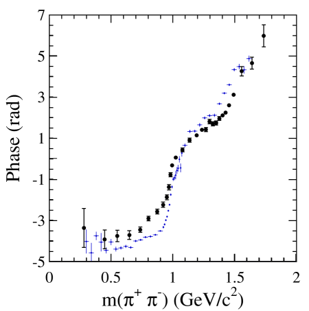
Figure 11: Comparison of the $\pi\pi$ S-wave phase as extracted from decays of $D_{s}$-mesons (BaBar Aubert et al. (2009a) - solid dots) and from a first freed-isobar analysis of the $(3\pi)^{-}$ system forming a $\pi(1800)$ (blue crosses) derived from Adolph et al. (2015). An arbitrary phase offset was added to the COMPASS data to roughly match the phase variation around $f_{0}(980)$ .

XII.1.2 Description of a resonance - poles

Until recent, almost all determinations of meson and heavy-baryon resonances and their parameters have been performed using “simple” mass fits based on Breit-Wigner amplitudes together with a coherent background amplitude (the parametrization of the latter is mostly empirical). Only elastic-scattering data have been used to extract pole information from the S-matrix. While experimentalists are exposed to much criticism for using Breit-Wigner amplitudes, few other methods have been on the market and are easily available. Although BaBar and COMPASS have started to use polynomials and $K$-matrix parametrizations for their fits, this work has not been concluded and there is a significant model dependence in the formulation of these analytic functions. Some more guidance and a list of “pros” and “cons” of different recipes, to which one can refer, would be very helpful. We see this as the only way to obtain process independent information, also referred to by the PDG.

XII.1.3 Threshold phenomena

With the appearance of $X,Y,Z_{c,b}$ and $P_{c}$-states and also recently, the $a_{1}(1420)$, the question of their nature dominates the discussion in hadron physics. This is particularly true for resonance structures appearing close to thresholds of pairs of much lighter mesons. Here, triangular or loop diagrams can be calculated (probably up to some overall amplitude factor) resulting in analytical amplitudes, which could be used by experimentalists in their mass-dependent fits, replacing the above mentioned pole descriptions. This would complete all analyses of new states in terms of well-motivated mass-dependent amplitudes.

XII.1.4 Non-resonant contributions in diffraction

Pion diffraction off nucleons always results in a superposition of production processes, e.g. Pomeron exchange and “Deck” effect, where the latter is modeled to proceed via pion-nucleon elastic scattering with Reggeon exchange at the nucleon-vertex and by the exchange of a pion to the “upper” pion vertex. The “Deck” process is thought to be the most prominent non-resonant contribution in diffraction. These production processes have different dependences on the four-momentum transfer $t^{\prime}$ to the target proton and thus may be disentangled by performing the PWA at various values of $t^{\prime}$. This may provide clearer access to resonances without the use of simplistic parametrizations of the non–resonant contribution, which is known to distort resonance signals. Here, a better model for the non–resonant production is required, which can be developed only if detailed information from “inside” the production amplitude is known. This task should be addressed jointly by theorists and experimentalists.

XII.2 Conclusion

Partial-wave analyses of various multi-body systems have reached a new level of accuracy and complexity. With much closer links to theoretical calculations, the extraction of physics information could be raised to a new level, namely (nearly) “universal” amplitudes. Extraction of pole parameters, the role of underlying dynamics and $CP$ violation based on calculable strong amplitudes could be much rewarding results. We are aware that substantial effort is ongoing already (see e.g. “white paper” Battaglieri et al. (2015)), but a worldwide coherent program, which includes heavy- and light-quark physics processes, could accelerate the development, for which theory is an absolutely necessary and crucial ingredient.

XIII CPT, Final State Interaction and CP Violation

T. Frederico^a, J. H. Alvarenga Nogueira^a, I. Bediaga^b, A. B. R. Cavalcante^b, and O. Lourenço^c

^aInstituto Tecnológico de Aeronáutica

DCTA, 12228-900, São José dos Campos, SP, Brazil

^bCentro Brasileiro de Pesquisas Físicas

LAFEX, 22290-180, Rio de Janeiro, RJ, Brazil

^cDepartamento de Ciências da Natureza, Matemática e Educação

CCA, Universidade Federal de São Carlos, 13600-970, Araras, SP, Brazil

The CPT invariance of the fundamental theory implies identical particle and antiparticle lifetimes. The partial decay widths of CP conjugate channels can be different due to CP violation (CPV), but in order to fulfill the CPT constraint their sum, namely the total width for particle and antiparticle, should be equal. Therefore, the amount of CPV in one channel should be compensated in other ones. The mechanism that allows the flow of CPV between different channels is the final state interaction (FSI), which couples different states in the decay channel. The discussion given in the following presents a CP asymmetry formula including resonances and FSI based on the CPT constraint.

The CP asymmetry formula is discussed in the lowest order in the strong interaction and decomposed in the two-body channels angular momentum. At the end of the section an expression for the CP asymmetry is provided for the decays channels $B^{\pm}\to\pi^{\pm}\pi^{+}\pi^{-}$ and $B^{\pm}\to K^{\pm}\pi^{+}\pi^{-}$. For this example, we parametrise the Dalitz plot with an isobar model, with Breit Wigner lineshapes for resonances like the $\rho$ and the $f_{0}(980)$, plus a non-resonant background. In addition, the contributions from the $\pi\pi\leftrightarrow KK$ coupled channel amplitude is taken into account.

We follow closely refs. Marshak et al. (1969); Branco et al. (1999); Bigi and Sanda (2000); Bediaga et al. (2014); Alvarenga Nogueira et al. (2015) to introduce our notation and the CPT constraint in $B$ meson decays. We start with the CPT invariance of the weak Hamiltonian $H_{w}$ and the strong Hamiltonian $H_{s}$, namely $(\mathcal{CPT})^{-1}H_{w,s}\mathcal{CPT}=H_{w,s}$. The hadron weak decay amplitude is obtained as the matrix element $\langle\lambda_{out}|H_{w}|h\rangle$, where the state $|\lambda_{out}\rangle$ carries the effect of the strong interaction between the hadrons in the final state. This is our main assumption.

The requirement of CPT invariance on the decay amplitude is $\langle\lambda_{out}|H_{w}|h\rangle=\chi_{h}\chi_{\lambda}\langle\overline{\lambda}_{in}|H_{w}|\overline{h}\rangle^{*}\,,$ where we used that the hadron state $|h\rangle$ transforms under CPT as ${\mathcal{CPT}}\,|h\rangle=\chi\langle\overline{h}|$, where $\overline{h}$ is the charge conjugate state and $\chi$ a phase. The completeness relation for the strongly interacting states in terms of the eigenstates of $H_{s}$, $|\lambda_{out}\rangle$, given by $\sum_{\bar{\lambda}_{out}^{\prime}}|\bar{\lambda}_{out}^{\prime}\rangle\langle\bar{\lambda}_{out}^{\prime}|$, and the hermiticity of $H_{w}$ implies that

$$\langle\lambda_{out}|H_{w}|h\rangle=\chi_{h}\chi_{\lambda}\sum_{\overline{\lambda}^{\prime}}S_{\overline{\lambda}^{\prime},\overline{\lambda}}\langle\overline{\lambda}^{\prime}_{out}|H_{w}|\overline{h}\rangle^{*}\,,$$ (30)

where $S_{\overline{\lambda}^{\prime},\overline{\lambda}}=\langle\overline{\lambda}^{\prime}_{out}|\overline{\lambda}_{in}\rangle=S_{\lambda^{\prime},\lambda}\$ defines the matrix elements of the S-matrix. These matrix elements contain the information about the distortion of the final state due to the strong interaction, related to the strong phase. Note that, the final state in general can have more than two particles, and therefore the strong phase in the general case is not restricted to be directly associated with only the two-body phase-shift.

The full widths of the decaying particle and its charge conjugate are identical, i.e., the mean life of the particle and its conjugate are equal. From the CPT invariance relation (30) and the hermiticity of $H_{w}$, one can easily prove that the sum of partial widths of the hadron and its charge conjugate are indeed equal (see for details ref. Bediaga et al. (2014)).

The expression (30) can be turned practical by introducing the expansion of the strongly interacting state as the free state $(\lambda_{0}\rangle)$ plus scattering corrections: $|\lambda_{out}\rangle=|\lambda_{0}\rangle+\dots$. The free state is the mesonic noninteracting state, which does not carry the distortion due to the strong force. Thus, we write that:

$$\langle\lambda_{out}|H_{w}|h\rangle=\chi_{h}\chi_{\lambda}\sum_{\overline{\lambda}^{\prime}}S_{\overline{\lambda}^{\prime},\overline{\lambda}}\langle\overline{\lambda}^{\prime}_{0}|H_{w}|\overline{h}\rangle^{*}+\cdots=\sum_{\lambda^{\prime}}\left(\delta_{\lambda^{\prime},\lambda}+i\,t_{\lambda^{\prime},\lambda}\right)\langle\lambda^{\prime}_{0}|H_{w}|h\rangle+\cdots\ ,$$ (31)

where we have used the CPT invariance of the weak Hamiltonian, i.e., $\langle\lambda_{0}|H_{w}|h\rangle=\chi_{h}\chi_{\lambda}\langle\overline{\lambda}_{0}|H_{w}|\overline{h}\rangle^{*}\,$, the CP invariance of the strong S-matrix, namely $S_{\lambda^{\prime},\lambda}=S_{\overline{\lambda}^{\prime},\overline{\lambda}}$ and we have written the S-matrix in terms of the scattering amplitude $t_{\lambda^{\prime},\lambda}$, as $S_{\lambda^{\prime},\lambda}=\delta_{\lambda^{\prime},\lambda}+i\,t_{\lambda^{\prime},\lambda}$. The decay amplitudes computed with the non interacting terms in (31) have the effect of CP violation and are written in general as a sum of two terms:

$$\langle\lambda_{0}|H_{w}|h\rangle=A_{0\lambda}+e^{-i\gamma}B_{0\lambda},\leavevmode\nobreak\ \leavevmode\nobreak\ \leavevmode\nobreak\ \text{ and }\leavevmode\nobreak\ \leavevmode\nobreak\ \leavevmode\nobreak\ \leavevmode\nobreak\ \langle\overline{\lambda}_{0}|H_{w}|\overline{h}\rangle=A_{0\lambda}+e^{+i\gamma}B_{0\lambda},$$ (32)

where $A_{0\lambda}$ and $B_{0\lambda}$ can be in principle associated with the tree and penguin amplitudes in the Bander-Silverman-Soni (BSS) model Bander et al. (1979). The BSS mechanism is the direct CPV due to the interference of the tree (weak phase) and penguin (strong phase) amplitudes leading to the same final state. Within the present framework we name the amplitudes $A_{0\lambda}$ and $B_{0\lambda}$, as partonic or source amplitudes. In the region of the Dalitz plot where the effects of the final state interaction and formation of resonances are small, the source amplitudes are directly accessible and are associated with the usual non-resonant background, although the source amplitudes, in principle, cover all the available phase-space. Substituting the source terms in (31) one has that:

$$\langle\lambda_{out}|H_{w}|h\rangle=\sum_{\lambda^{\prime}}\left(\delta_{\lambda^{\prime},\lambda}+i\,t_{\lambda^{\prime},\lambda}\right)\left(A_{0\lambda}+e^{-i\gamma}B_{0\lambda}\right)+\cdots\ ,$$ (33)

which gives for the CP asymmetry , $\Delta\Gamma_{\lambda}=|\langle\lambda_{out}|H_{w}|h\rangle|^{2}-|\langle\overline{\lambda}_{out}|H_{w}|\overline{h}\rangle|^{2}$, computed to leading order in the hadronic interaction, the following expression:

$$\Delta\Gamma_{\lambda}=4(\sin\gamma)\,\mbox{Im}\Bigg{\{}\left(B_{0\lambda}\right)^{*}A_{0\lambda}+i\sum_{\lambda^{\prime}}\left[\left(B_{0\lambda}\right)^{*}t_{\lambda^{\prime},\lambda}\,A_{0\lambda^{\prime}}-\left(B_{0\lambda^{\prime}}\,t_{\lambda^{\prime},\lambda}\right)^{*}A_{0\lambda}\right]\Bigg{\}},$$ (34)

where $\lambda^{\prime}$ labels each state coupled to the decay channel $\lambda$ by the strong interaction. The last two terms in the right-hand side of eq. (34) can be interpreted as the “compound” CP asymmetry Atwood and Soni (1998); *Soni2005_b. These two contributions cancel each other when summed in $\lambda$ (note that an integration over the phase-space is also implicit) resulting in the CPT condition, $\sum_{\lambda}\Delta\Gamma_{\lambda}=0$, if the source amplitudes satisfy: $\sum_{\lambda}\mbox{Im}\left[\left(B_{0\lambda}\right)^{*}A_{0\lambda}\right]=0,$ which is a consequence of the CPT constraint at the microscopic level, e.g., as expressed by the tree and penguin amplitudes in the BSS model, that should be valid in the absence of final state interactions. This term was neglected by Wolfenstein Wolfenstein (1991), which corresponds to the trivial solution of this equality, assuming that the phase difference between the two CP-conserving amplitudes is zero for all decay channels. Therefore, if we have only two decay channels, namely, $\lambda$ and $\lambda^{\prime}$, which are coupled by the strong interaction, we can write:

$$\Delta\Gamma_{\lambda}=4(\sin\gamma)\,\mbox{Re}\Big{\{}\left(B_{0\lambda}\right)^{*}t_{\lambda^{\prime},\lambda}\,A_{0\lambda^{\prime}}-\left(B_{0\lambda^{\prime}}\,t_{\lambda^{\prime},\lambda}\right)^{*}A_{0\lambda}\Big{\}}=-\Delta\Gamma_{\lambda^{\prime}}\,,$$ (35)

To derive the above expression we used $t_{\lambda^{\prime},\lambda}=t_{\lambda,\lambda^{\prime}}$. The relation (35) has been used in Ref. Bediaga et al. (2014) for a qualitative analysis of the large CP violation effects observed by the LHCb collaboration  in charmless three-body $B^{\pm}$ decays Aaij et al. (2013d). The focus of the study is the decay channels $B^{\pm}\to K^{\pm}K^{+}K^{-}$ and $B^{\pm}\to K^{\pm}\pi^{+}\pi^{-}$ in the low $K^{+}K^{-}$ and $\pi^{+}\pi^{-}$ mass regions between 1 and 1.6 GeV, where these channels are coupled by the strong interaction Grayer et al. (1974); Cohen et al. (1980).Expression (35) shows that apart from a phase-space factor, the asymmetries in these channels are proportional to $\sqrt{1-\eta^{2}}\cos\left(\delta_{KK}+\delta_{\pi\pi}+\Phi\right)$. This factor arises from the magnitude and phase of the $\pi\pi\to KK$ transition amplitude Peláez and Ynduráin (2005); *pelaprd05_b: $\eta$ is the inelasticity parameter and $\delta_{\pi\pi(KK)}$ are the isoscalar spin zero phase-shifts. A more detailed analysis is presented in Alvarenga Nogueira et al. (2015) based on the recent experimental findings of LHCb Aaij et al. (2014b). Both analyses based on Eq. (35) led to the conclusion that the “compound contributions are essential to form the observed pattern of the CP asymmetry data.

We now discuss equation (35) for the particular case when $A_{0\lambda}=0$ in the two-channel case, which gives that: $\Delta\Gamma_{\lambda}=4(\sin\gamma)\,\mbox{Re}\{\left(B_{0\lambda}\right)^{*}t_{\lambda^{\prime},\lambda}\,A_{0\lambda^{\prime}}\}\,.$ In this configuration, still, a CP asymmetry can appear due to the interference of two terms, where one of them arises from the strong coupling between the channels $\lambda$ and $\lambda^{\prime}$ and the other is the one related with the weak phase. Now consider a $B^{\pm}$ decay channel where the penguin (tree) contribution is negligible, while in the corresponding coupled channel it is the opposite, i.e., the tree (penguin) contribution can be neglected. Then, the weak CP violating phase comes only through one channel and for the CP asymmetry to be visible, the interference has to occur between amplitudes originating in different channels, coupled by the strong interaction. In this case, FSI are the dominant mechanism leading to CP violating interference effects.

For more detailed applications, the expression (31) has to include resonances formed in the partonic process, like for example $B\to\pi\rho$ (see Alvarenga Nogueira et al. (2015)). To take into account resonances the amplitudes $A_{0\lambda}$ and $B_{0\lambda}$ are separated in two parts:

$$A^{J}_{0\lambda}=A^{J}_{0\lambda NR}+\sum_{R}A^{J}_{0\lambda R}\quad\mbox{and}\quad B^{J}_{0\lambda}=B^{J}_{0\lambda NR}+\sum_{R}B^{J}_{0\lambda R}\,,$$ (36)

where the subscripts $R$ and $\mathit{NR}$ mean resonant and nonresonant channels, respectively. The label $J$ indicates the spin of the two-body state. Accounting for (36) the decay amplitude in Eq. (33) can be generalized to:

$$\mathcal{A}^{\pm}_{LO} =\sum_{J}\left[\sum_{R}A^{J}_{0\lambda R}+A^{J}_{0\lambda NR}+\right.\left.e^{\pm i\gamma}\left(\sum_{R}B^{J}_{0\lambda R}+B^{J}_{0\lambda NR}\right)\right]+$$

$$+i\sum_{\lambda^{\prime},J}t^{J}_{\lambda^{\prime},\lambda}\left[\sum_{R}A^{J}_{0\lambda^{\prime}R}+A^{J}_{0\lambda^{\prime}NR}+\right.\left.e^{\pm i\gamma}\left(\sum_{R}B^{J}_{0\lambda^{\prime}R}+B^{J}_{0\lambda^{\prime}NR}\right)\right],$$ (37)

where in the expression above the strong scattering amplitude $t_{\lambda^{\prime},\lambda}$ is considered to leading order (LO). In addition, the source resonant terms $A^{J}_{0\lambda R}$ and $B^{J}_{0\lambda R}$ should be interpreted as bare amplitudes, which are formed directly at the partonic level where the two-hadron rescattering process is not yet included. Therefore, the Breit-Wigner (BW) amplitudes in each term are identified with

$$(1\,+\,i\,t^{J}_{\lambda\lambda})A^{J}_{0\lambda R}\to a_{0}^{R}F_{R\,\lambda}^{BW}P_{J}(\cos\theta)\quad\mbox{and}\quad(1\,+\,i\,t^{J}_{\lambda\lambda})B^{J}_{0\lambda R}\to b_{0\lambda}^{R}F_{R\,\lambda}^{BW}P_{J}(\cos\theta),\quad$$ (38)

where $J$ is the spin of the resonance decaying to two spin zero particles and $P_{J}(\cos\theta)$ is the $J^{th}$ order Legendre polynomial and $\theta$ is the helicity angle between the same-charge particles in the Gottfried-Jackson frame.

After substituting (38) in (37), we get that

$$\mathcal{A}^{\pm}_{LO}=\sum_{J\,R}\left(a_{0\lambda}^{R}+e^{\pm i\gamma}b_{0}^{R}\right)F_{R\,\lambda}^{BW}P_{J}(\cos\theta)+\sum_{J}\left(A^{J}_{0\lambda NR}+e^{\pm i\gamma}B^{J}_{0\lambda NR}\right)+i\sum_{\lambda^{\prime},J}t^{J}_{\lambda^{\prime},\lambda}\left(A^{J}_{0\lambda^{\prime}NR}+e^{\pm i\gamma}B^{J}_{0\lambda^{\prime}NR}\right),$$ (39)

where the first and second term in the right-hand side are associated with the isobar model. The second term is the source amplitude for the final state channel, and the third one includes the hadronic interaction among the two of the hadrons with angular momentum $J$. We should note that the third term in eq. (39) could also include a resonance in channel $\lambda^{\prime}$, which can decay to channel $\lambda$ due to the coupling between these states by the strong interaction, although we have not included this possibility in the expression of the decay amplitude. The resulting CP asymmetry from eq. (39), considering terms only in the LO on the strong scattering amplitude, can be cast in the following form:

$$\Delta\Gamma_{\lambda}=\Gamma\left(h\to\lambda\right)-\Gamma(\overline{h}\to\overline{\lambda})=\\ =4(\sin\gamma)\,\sum_{J\,J^{\prime}}\mbox{Im}\left\{\left(\sum_{R}b_{0\lambda}^{R}F_{R\lambda}^{BW}P_{J}(\cos\theta)+B^{J}_{0\lambda NR}\right)^{*}\left(\sum_{R^{\prime}}a_{0\lambda}^{R^{\prime}}F_{R^{\prime}\lambda}^{BW}P_{J^{\prime}}(\cos\theta)+A^{J^{\prime}}_{0\lambda NR}\right)+\right.\\ +\,i\sum_{\lambda^{\prime}}\left(\sum_{R}b_{0\lambda}^{R}F_{R\lambda}^{BW}P_{J}(\cos\theta)+B^{J}_{0\lambda NR}\right)^{*}\,t^{J^{\prime}}_{\lambda^{\prime},\lambda}\,\left(\sum_{R^{\prime}}a_{0\lambda^{\prime}}^{R^{\prime}}F_{R^{\prime}\lambda^{\prime}}^{BW}P_{J^{\prime}}(\cos\theta)+A^{J^{\prime}}_{0\lambda^{\prime}NR}\right)+\\ \left.-\,i\sum_{\lambda^{\prime}}\left(\sum_{R^{\prime}}b_{0\lambda^{\prime}}^{R^{\prime}}F_{R^{\prime}\lambda^{\prime}}^{BW}P_{J^{\prime}}(\cos\theta)+B^{J^{\prime}}_{0\lambda^{\prime}NR}\right)^{*}\,\left[t^{J^{\prime}}_{\lambda^{\prime},\lambda}\right]^{*}\,\left(\sum_{R}a_{0\lambda}^{R}F_{R\lambda}^{BW}P_{J}(\cos\theta)+A^{J}_{0\lambda NR}\right)\right\}.$$ (40)

The subindex $\lambda$ also includes different kinematical regions of the three-body channel. Since we have introduced the Breit-Wigner amplitudes in the decay amplitude $(F_{R^{\prime}\lambda^{\prime}}^{BW})$, the CPT constraint has to be checked in the actual fit, i.e., if $\sum_{\lambda}\Delta\Gamma_{\lambda}=0$ is satisfied when one takes into account the integration over the phase-space besides the sum over all decay channels in the sum of $\lambda$. In the fitting procedure performed in Alvarenga Nogueira et al. (2015), we kept only terms that are consistent with the CPT constraint.

The non-resonant source terms, $A^{J^{\prime}}_{0\lambda^{\prime}NR}$ and $B^{J^{\prime}}_{0\lambda^{\prime}NR}$, can contain a form factor like $\left(1+\frac{s}{\Lambda^{2}_{\lambda}}\right)^{-1}$ or similar to parametrize the dependence on the square mass of the two particle system (either $\pi\pi$ or $KK$) produced by the short-range dynamics. Such form factor is associated with the partonic decay amplitude that produces the three-meson final state. In the production process, the relative momentum between the pair of mesons is distributed among the quarks in the momentum loop within the microscopic amplitude computed with the tree and penguin diagrams. Therefore, by changing the relative momentum between the mesons in the final state the internal structure of the mesons involved in the initial and final states are probed. In general, the non resonant amplitude should depend on the two kinematically independent Mandelstam variables ;for simplicity, we chose only one of them in the example given above. The suggestion of a power-law form just reflects the hard momentum structure of the mesons involved in the decay Brambilla et al. (2014). For example, by looking at the tree diagram, one observes that the decay of the $b-$quark in in its rest frame, produces a fast light quark and a pion back to back. The light quark has to share its momentum with a slow antiquark, which is driven by the gluon exchange and is damped by a momentum power-law form. A similar reasoning can be applied to the penguin diagram.

Expression (40) for the CP asymmetry is worked out for the example of a charmless three-body $B$ decay. It is expanded in a form where the unknown parameters are exposed in such a way that they can be easily fit to experimental data,

$$\Delta\Gamma_{\lambda} =\frac{\mathcal{B}\cos[2\delta_{\pi\pi}(s)]\sqrt{1-\eta^{2}(s)}}{\left(1+\frac{s}{\Lambda^{2}_{\lambda}}\right)\left(1+\frac{s}{\Lambda^{2}_{\lambda^{\prime}}}\right)}+|F^{\rm BW}_{\rho}(s)|^{2}k(s)\cos\theta\left\{\frac{\mathcal{D}(m^{2}_{\rho}-s)}{1+\frac{s}{\Lambda^{2}_{\lambda}}}+\frac{\mathcal{E}m_{\rho}\Gamma_{\rho}(s)}{1+\frac{s}{\Lambda^{2}_{\lambda}}}\right\}$$ (41)

$$+ F^{\rm BW}_{\rho}(s)|^{2}|F^{\rm BW}_{f}(s)|^{2}k(s)\cos\theta\times$$

$$\times \left\{\mathcal{F}[(m_{\rho}^{2}-s)(m_{f}^{2}-s)+m_{\rho}\Gamma_{\rho}(s)m_{f}\Gamma_{f}(s)]\right.+\left.\mathcal{G}[(m_{\rho}^{2}-s)m_{f}\Gamma_{f}(s)-m_{\rho}\Gamma_{\rho}(s)(m_{f}^{2}-s)]\right\}.$$

In the expression above, $\lambda$ is associated to $\pi^{\pm}\pi^{+}\pi^{-}$ or $K^{\pm}\pi^{+}\pi^{-}$, and $\lambda^{\prime}$ to $\pi^{\pm}K^{+}K^{-}$ or $K^{\pm}K^{+}K^{-}$. The Mandelstam variable $s$ is the interacting pair square mass. All parameters $\mathcal{B},\,\mathcal{D},\,\mathcal{E},$ $\,\mathcal{F}$ and $\mathcal{G}$ are related only with the partonic amplitudes $A^{J}_{0\lambda}$ and $B^{J}_{0\lambda}$ and with the phase $\gamma$. These relations are discussed in more detail in Ref. Alvarenga Nogueira et al. (2015). The $F^{\rm BW}(s)$ is the relativistic Breit-Wigner and $\Gamma(s)$ is the width, and for $\pi^{\pm}K^{+}K^{-}$ or $K^{\pm}K^{+}K^{-}$ channels, only $\mathcal{B}$ is non zero. Eq. (41) contains interferences involving the non-resonant background, the resonances $\rho(770)$ and $f_{0}(980)$ and the S-wave $KK\rightarrow\pi\pi$ amplitude. The parameters $\eta(s)$ and $\delta_{\pi\pi}$ are the inelasticity parameter and isoscalar s-wave $\pi\pi$ phase-shift, respectively Peláez and Ynduráin (2005); *pelaprd05_b. All terms that violate CPT when integrated over the Dalitz give non vanishing contribution, were completely ignored in the above formula.

In the future, the analysis of the CP asymmetries in charmless $B$ decays will be extended to include corrections induced by the three-body rescattering processes following the same approach that has been applied in the charm sector to $D\to K\pi\pi$ decay (see Magalhães et al. (2011); Guimarães et al. (2014); Frederico et al. (2014) ).

Acknowledgments

JHAN acknowledges the support from Fundação de Amparo à Pesquisa do Estado de São Paulo (FAPESP), Grant No. 2014/19094-8. We also thank the partial support from Conselho Nacional de Desenvolvimento Científico e Tecnológico (CNPq).

XIV Analytical improvements to Breit-Wigner isobar models

Adam P. Szczepaniak^a,b,c

^aCenter for Exploration of Energy and Matter, Indiana University, Bloomington, IN 47403 ^bPhysics Department, Indiana University, Bloomington, IN 47405, USA ^cThomas Jefferson National Accelerator Facility, Newport News, VA 23606, USA

We discuss the derivation and properties of the general representation of partial wave amplitudes in the context of improving the models currently used in analysis of three particle Dalitz distributions.

XIV.1 introduction

In this note, after a brief introduction to aspects of $S$-matrix theory relevant in the analysis of three particle Dalitz plots, I focus on properties of Breit-Wigner (BW) amplitudes and the isobar model in general. I discuss the LHCb analysis model in the context of a general isobar-type approximation and show, for example, which features of the BW amplitude, e.g. barrier factors, Blatt-Weisskopf factors, etc. are universal and which are not, i.e. are process dependent. The possibility of extending the BW description in a way that is consistent with analyticity, unitarity, and even crossing would allow to access systematic uncertainties in data analysis. I concentrate on spinless particles. Spin introduces kinematical complexities but does not affect how unitarity, analyticity, and crossing are implemented, at least for a finite set of partial waves.

XIV.2 Kinematical vs Dynamical Singularities

We are interested in amplitudes describing a decay of a quasi-stable particle $D$ with mass $M$ to three distinguishable particles $A,B,C$

$$D\to A+B+C$$ (42)

The decay amplitude depends on particle helicities, $\lambda_{i}$, $i=A,B,C,D$, and three Mandelstam invariants, which we define as $s=(p_{A}+p_{B})^{2}$, $t=(p_{B}+p_{C})^{2}$ and $u=(p_{A}+p_{C})^{2}$. The invariants are kinematically constrained by $s+t+u=\sum_{i}m_{i}^{2}$. Analytical $S$-matrix theory states that, besides the decay channel, the same amplitude describes each of the three two-to-two scattering process, i.e the $s$-channel reaction $D+\overline{C}\to A+B$, (bar denotes an antiparticle) as well as the $t$ and $u$ channel scattering. What this means in practice is the following. For each combination of helicities there is an analytical function $A_{\lambda_{i}}(s,t,u)$ of the three complex Mandelstam variables and complex $M^{2}$, such that the three physical scattering amplitudes and the decay channel amplitude correspond to the limit of $A_{\lambda_{i}}$ when $s,t,u,$ and $M$ approach the real axis in the physical domain of the corresponding reaction. This is the essence of crossing symmetry. In general crossing mixes helicity amplitudes and leads to complicated relations for helicity amplitudes. Furthermore, helicity amplitudes have kinematical singularities in the Mandelstam variables. Despite such complexities it is possible to come up with parameterizations of helicity amplitudes that take into account both kinematical and dynamical constraints Martin and Spearman (1970). On the other hand it is also useful to consider the covariant from i.e. a representation of helicity amplitudes in terms of Lorentz-Dirac factors that describe wave functions of the free particles participating in the reaction. The advantage of the covariant representation is that the scalar functions multiplying all independent covariants are simply related by crossing and are free from kinematical singularities. At the end of the day one still needs the helicity amplitudes for partial wave analysis. In  Danilkin et al. (2015) the reaction $\omega\to\pi^{+}\pi^{-}\pi^{0}$ was studied and this example provides a good illustration of the issues discussed above.

The main postulate of relativistic reaction theory is that reaction amplitudes are analytical functions of kinematical variables. It follows from Cauchy’s theorem that an analytical function is fully determined by its domain of analyticity, i.e. location of singularities. Thus knowing amplitude singularities allows to determine the amplitude elsewhere, including the various physical regions. In S-matrix theory it is assumed that all singularities can be traced to unitarity. In the absence of an explicit solution to the scattering problem in QCD, analyticity and unitarity provide the least model dependent description of hadron scattering.

Unitarity operates in any of the Mandelstam variables. In the $s$-channel the physical domain is located on the positive real axis in the $s$-plane above the elastic threshold. Unitarity makes amplitudes singular at each open channel threshold, the singularity being of the square-root type. The same happens in variables $u$ and $t$. The amplitude also has singularities in the variable $M$ since it represents an unstable channel. In studying a particular decay process, e.g. $J/\psi\to 3\pi$, $M$ is fixed in a very narrow range (within the width of the $J/\psi$), and dependence on $M$ is effectively fixed and its singularity structure irrelevant.

In general, it is not known how to write an amplitude that has correct unitarity constraints in two or more overlapping channels. The reason being that it is only simple to implement unitarity on partial waves where it is an algebraic constraint. A single partial wave in one channel corresponds to an infinite number of partial waves in another one thus imposing unitarity on say both $s$ and $t$-channel partial waves simultaneously requires an infinite number of partial waves. Regge theory extends the concept of analytical continuation to the angular momentum variable of partial waves. Singularities in the angular momentum plane e.g. Regge poles, determine the behavior of infinite sums of partial waves, thus Regge theory is used to implement cross channel unitarity.

In general, amplitude singularities are known only in a limited domain, but as long as they dominate in a kinematical region of interest one may be able to construct a realistic amplitude model. Amplitude models fall into two main categories. One is that of dual models, e.g. the Veneziano model and the other is the isobar model category, e.g. the Khuri-Treiman model. Dual models attempt to incorporate $S$-matrix constraints directly on the full amplitude that depends on the Mandelstam variables. Since isobar is synonymous with a partial wave, isobar models are models based on a (truncated) partial wave expansion.

In the following I will discus the isobar model in some detail since this is almost exclusively the model used at present in analyses of three particle Dalitz distributions.

XIV.3 The Breit-Wigner amplitude

In the Breit-Wigner formula, a partial wave, $f_{l}(s)$ is approximated by a pole in $s$ located in the complex energy plane at $s_{P}=Res_{P}-i\mathit{Im}s_{P}$,

$$f^{p}_{l}(s)\propto\frac{1}{s_{P}-s}$$ (43)

The real and imaginary parts are related to the mass, $M=\sqrt{Re\,s_{P}}$ and the width, $\Gamma=Im\,s_{P}/M$ of a resonance. For comparison with experiment a reaction amplitude is evaluated at physical, real values of kinematical variables e.g when $s$ approaches the real axis from above. The contribution form a BW pole to a partial cross section, $\sigma_{l}$ is proportional to

$$\sigma_{l}\propto\lim_{\epsilon\to 0}|f^{p}_{l}(s+i\epsilon)|^{2}\propto\frac{1}{(s-M^{2})^{2}+(M\Gamma)^{2}}.$$ (44)

Since the resonance pole is located in the complex s-plane, on the real s-axis, where experimental data is taken, it produces a smooth variation in the cross section. The closer the pole is to the real axis, i.e. the smaller the resonances width, the more rapid is the variation in cross section or event distribution. It is worth keeping in mind that once energy is considered as a complex variable any variation of the reaction amplitude in the physical region can be traced to the existence of singularities in the complex energy plane e.g. a pole as in the BW formula.

XIV.4 Unitarity and the Breit-Wigner amplitude

The BW formula of Eq. (43) is an analytical function of $s$ except for a single pole at $s=s_{P}$. How does unitarity constrain the BW pole? Resonance decay is possible because of open channels and it is unitarity that controls the distribution of probability across decays. It thus follows that unitarity must constrain resonance decay widths and thus the imaginary part of the BW pole. But Eq. (43) is only an approximation to the “true”, unitary amplitude valid for $s$ near the position of the complex pole. Since unitarity operates in the physical domain, i.e. on the real axis, the constraint of unitarity on the “true” amplitude is lost in the pole approximation, i.e. at a finite distance from the real axis. In this case implementing unitarity is related to using energy dependent widths.

Suppose the lowest mass open channel is a state of particles $A$ and $B$ with threshold at $s=s_{th}=(m_{A}+m_{B})^{2}$. In the mass range between $s_{th}$ and the first threshold, unitarity constrains the “true” amplitude to satisfy

$$Im\hat{f}_{l}(s)=\hat{t}^{*}_{l}(s)\rho_{l}(s)\hat{f}_{l}(s).$$ (45)

Here $\hat{f}_{l}(s)=f_{l}(s)/(aq)^{l}$ and $\hat{t}_{l}(s)=t_{l}(s)/(aq)^{2l}$ are the $s$-channel reduced partial waves representing production of $AB$ in $D+\overline{C}\to A+B$ and elastic $A+B\to A+B$ scattering, respectively. Near threshold $q\to 0$, with $q$ being the relative momentum between $A$ and $B$ in the $s$-channel center of mass frame, partial waves vanish as $(aq)^{l}$, where $a$ is given by the position of the lowest mass singularity in the crossed channels, i.e. the range of interaction. $\rho_{l}(s)$ is a known kinematical function describing the two-body phase space. It has a square-root branch point at $s=s_{tr}$. As $s$ increases beyond the first inelastic threshold, $Im\hat{f}_{l}(s)$ receives a “kick” from another square-root type singularity form channel openings and the r.h.s of Eq. (45) needs to be modified. Eventually three and more particle channels open. In practice unitarity is a useful constraint in a limited energy range that covers a small number of open channels e.g. close to the elastic threshold. Replacing, in Eq. (45), $\hat{f}_{l}$ by $\hat{t}$ one obtains the unitarity relation for the elastic $A+B\to A+B$ partial waves in the elastic region,

$$Im\hat{t}_{l}(s)=|\hat{t}(s)|^{2}\rho_{l}(s).$$ (46)

Above the inelastic threshold the r.h.s of Eq. (46) should be modified as discussed above. In case there is a finite number $N$ of relevant inelastic channels, the unitarity condition can be expressed in a matrix form

$$Im\hat{t}_{l,ij}(s)=\sum_{k}\hat{t}_{l,ik}^{*}(s)\rho_{l,k}(s)\hat{t}_{kj}(s)$$ (47)

where $\hat{t}_{l,ij}(s)=t_{l}(s)/(aq)^{l_{i}}(aq)^{l_{j}}$ and $\rho_{l,k}(s)$ is the appropriate, reduced phase space in channel $k$. The unitarity relation for $\hat{f}_{l,i}(s)$ takes on a similar form,

$$Im\hat{f}_{l,i}(s)=\sum_{k}\hat{t}_{l,ik}^{*}(s)\rho_{l,k}(s)\hat{f}_{k}(s).$$ (48)

For a given $\hat{t}_{l}(s)$, the analytical amplitude $\hat{f}_{l}(s)$ that satisfies Eq. (45) can be written as

$$\hat{f}_{l}(s)=\hat{t}_{l}(s)G_{l}(s)$$ (49)

and sometimes the so-called Muskhelishvili-Omnes function is used instead of $\hat{t}_{l}(s)$ on the r.h.s of Eq. (49) Pham and Truong (1977). The function $G_{l}(s)$ is an analytical function of $s$ with cuts except on the real axis in the elastic region. The latter are accounted for by the elastic amplitude $t_{l}(s)$. The singularities of $G_{l}(s)$ correspond to the (often unknown) contributions from the unitarity-imposed left hand cuts cuts that exist in the crossed, $t$ and $u$ channels. The inelastic contributions i.e. right cuts in $\hat{f}_{l}$ are related to the inelastic contributions to the amplitude $\hat{t}_{l}(s)$ which is easy to show if the matrix representation is used,

$$\hat{f}_{l,i}=\sum_{k}\hat{t}_{l,ik}G_{l,k}(s)$$ (50)

and with the functions $G_{l,k}(s)$ bearing only left hand cuts. Now we go back to the pole formula. From Eq. (45) it follows that poles of the production amplitude $\hat{f}_{l}$ are also poles of $\hat{t}_{l}$. This is because no resonance poles appear on sheets connected to the left hand cuts Gribov (2009). Since $\hat{t}_{l}(s)$ satisfies Eq. (46) it can be shown that the most general parametrization has the form,

$$t_{l}(s)=\frac{1}{C_{l}(s)-I_{l}(s)}$$ (51)

which in the inelastic case generalizes to the matrix form

$$t_{l,ij}(s)=[C_{l}(s)-I_{l}(s)]^{-1}_{ij}$$ (52)

with $C_{l}$ and $I_{l}$ becoming $N\times N$ matrices in the channel space. The function $C_{l}(s)$ ($C_{l,ij}(s)$) has similar properties to the function $G_{l}(s)$ ($G_{l,i}(s)$) in Eq. (49), i.e. it is real for real $s$ in the elastic region and have only left hand cuts. The function $I_{l}(s)$ is a known analytical function i.e. the Chew-Mandelstam function, with its imaginary part for real $s$ given by $ImI_{l}(s)=\rho_{l}(s)$. The reason why the analytical solution of Eq. (46) is more complicated than that of Eq. (45), is that the former is a non-linear relation for the amplitude. It is easy to check that this equation becomes a linear condition for the inverse of $\hat{t}_{l}$ and this is the reason why dependence on phase space appears in the denominator in Eq. (51). It is straightforward to check that Eq. (51) satisfies Eq. (45), or in the inelastic case, its matrix generalization. The presence of “denominators” in amplitudes are a direct consequence of unitarity and so are the resonance poles, which correspond to zeros of the denominators.

One immediately recognizes that the $K$-matrix, or the $K$ function in the elastic case, corresponds to

$$K^{-1}_{l}(s)=C_{l}(s)-ReI_{l}(s).$$ (53)

Since the real part of a function is not an analytical function, an analytical approximation to the $K$ matrix violates analyticity of the amplitude and may lead to spurious “kinks” from square-root unitarity branch points in the physical region. It is much better to use Eq. (51), aka the Chew-Mandelstam representation, with the analytical ($K$-matrix type) parametrization reserved for the analytical function $C_{l}(s)$.

Combining Eq. (51) with Eq. (49) one obtains

$$\hat{f}_{l}(s)=\frac{G_{l}(s)}{C_{l}(s)-I_{l}(s)}$$ (54)

or in the matrix form for the inelastic case

$$\hat{f}_{l,i}(s)=\sum_{k}[C_{l}(s)-I_{l}(s)]^{-1}_{i,k}G_{l,k}.$$ (55)

Now we can finally see how the BW pole formula of Eq. (43) emerges. Suppose in Eq. (54) the denominator vanishes at some complex $s=s_{p}$. Near the pole of $\hat{f}_{l}$

$$\hat{f}_{l}(s)\sim\frac{\beta_{l}}{s-s_{p}}$$ (56)

where

$$\beta_{l}=G_{l}(s_{p})/(C^{\prime}_{l}(s_{p})-I^{\prime}_{l}(s_{p})).$$ (57)

In the inelastic case the role of the denominator in the r.h.s of Eq. (54) is played by the determinant of the $N\times N$ matrix $[C_{l}(s)-I_{l}(s)]$. Even though the residue of the pole $\beta_{l}$ is in general a complex number, it can be shown that only its magnitude is to be related with a coupling of a resonance to a decay channel Gribov (2009). The residue $\beta_{l}$ should be distinguished from the numerator $G_{l}(s)$. The latter is energy dependent and represents the production amplitude of the final state $A+B$ given the initial state $D+\overline{C}$. The former is a number representing the product of couplings of the resonance to the initial and final states.

Finally we “derive” the more familiar BW formula, with energy dependent widths. In the “LHCb” notation

$$f^{LHCb}_{l_{s}}(s)=F_{l_{s}}(q)R_{l_{s}}(s)F_{l_{t}}(p)$$ (58)

so that the reduced amplitude is given by

$$\hat{f}^{LHCb}_{l_{s}}(s)=\frac{F_{l_{s}}(q)}{(aq)^{l_{s}}}R_{l_{s}}(s)F_{l_{t}}(p)$$ (59)

where $q=q(s)$ is the decay channel relative momentum between $A$ and $B$ and $p=p(s)$ is the decay channel relative momentum between the $(AB)$ pair and the spectator particle $C$. For comparison with the analysis given above all that is needed is to replace the decay channel expressions for $q$ and $p$ by the $s$-channel ones. The function $F_{l}(x)$ is a product of an angular momentum barrier factor $x^{l}$ and a Blatt-Weisskopf factor

$$F_{l}(x)=(ax)^{l}F^{\prime}_{l}(x)$$ (60)

where, for example,

$$F^{\prime}_{2}(q)=\sqrt{\frac{13}{((aq)-3)^{2}+9(aq)}}$$ (61)

The propagator $R_{l_{s}}(s)$ is given by

$$R_{l_{s}}(s)=\frac{1}{m_{r}^{2}-s-i\rho_{l_{s}}(s)X(p)}$$

$$=\frac{1}{X(p)(C^{LHCb}(s)-i\rho_{l_{s}}(s))},\,C^{LHCb}(s)\equiv\frac{m_{r}^{2}-s}{X(p)}$$

so that one can rewrite the LHCb amplitude model as

$$\hat{f}^{LHCb}_{l_{s}}(s)=\frac{G^{LHCb}_{l_{s}}(s)}{C^{LHcB}(s)-i\rho_{l_{s}}(s)}$$ (63)

where

$$G^{LHCb}_{l_{s}}(s)=\frac{F^{\prime}_{l_{s}}(q)F_{l_{t}}(p)}{X(s)}.$$ (64)

Eq. (63) is a specific case of Eq. (54). It is in fact the $K$ matrix (function) approximation since only the imaginary part, $\rho_{l_{s}}(s)$ of the dispersive integral $I_{l}(s)$ is used. The functions $C_{l}$ and $G_{l}$ containing, through left hand cuts, physics of elastic production of $AB$ in $A+B\to A+B$ and in decay $D\to A+B+C$, respectively, have been replaced by a specific product of Blatt-Wisskopf factors. The latter originate from a potential model in non-relativistic scattering and at best can be considered as a crude approximation. In precision data analysis they should be replaced by a more flexible parametrization. In LHCb, analysis contributions from several poles are included by adding BW amplitudes. Eq. (54) shows how all such poles need to appear as zeros of the common denominator. Finally the matrix representation of Eq. (55) is the correct formula for dealing with multiple channels.

XIV.5 Combining $s$, $t$, and $u$, channel isobars and corrections to the isobar model

In the previous section we discussed how the energy dependent BW amplitude is related to the general expression for the partial wave. Here we discuss how the partial wave amplitudes build the full amplitude in the decay channel.

In the scattering domain of the $s$-channel, the partial wave expansion of the full amplitude converges and a finite number of partial waves waves may give a good approximation to the whole sum. Energy dependence of individual partial waves can be represented using expressions like the one in Eq. (49) or Eq. (50). In a decay channel, the partial wave series also converges, but one cannot simply replace the one sum but the other. This is because the decay channel partial waves have extra ”complexity” compared to the scattering channel, due to $t$ and $u$ channel singularities, i.e. resonances begin in the physical region. Ignoring spins of external particles, the $s$-channel partial wave series is given by

$$A(s,t,u)=\frac{1}{4\pi}\sum_{l=0}^{\infty}(2l+1)f_{l}(s)P_{l}(z_{s}).$$ (65)

On the r.h.s the dependence on $t$ and $u$ is algebraic, through $z_{s}$ and the rotational functions. Thus in the physical domain of the decay, the $s$-channel series diverges because the l.h.s has singularities in $t$ and $u$. Furthermore, it follows that any truncated, finite set of $s$-channel partial waves cannot reproduce $t$ or $u$-channel singularities, e.g. resonance which appear inside the Dalitz plot. These issues are resolved in the isobar model by replacing the infinite number of $s$-channel partial waves by a finite set and adding a (finite) set of $t$ and $u$ channel partial waves. Thus the amplitude has a mixed form that includes partial waves (isobars) in the three channels simultaneously,

$$A(s,t,u)=\frac{1}{4\pi}\sum_{l=0}^{L_{max}}(2l+1)a^{(s)}_{l}(s)P_{l}(z_{s})+(s\to t)+(s\to u)$$ (66)

We refer to $a^{(s)}_{l}(s)$ as the isobaric amplitude in the $s$-channel and analogously, $a^{(t)}_{l}(t)$ and $a^{(u)}_{l}(u)$ are the isobaric amplitudes in the $t$ and $u$-channels, respectively. In a typical Dalitz plot analysis, the isobaric amplitudes are parametrized using the energy dependent BW amplitudes discussed in the previous sections.

Projecting the r.h.s of Eq. (66) into the $s$-channel gives the $s$-channel partial waves, which we denoted by $f_{l}(s)$,

$$f_{l}(s)=a^{(s)}_{l}(s)$$

$$+\frac{1}{2}\int_{-1}^{1}dz_{s}P_{l}(z_{s})\sum_{l^{\prime}=0}^{L_{max}}(2l^{\prime}+1)a^{(t)}_{l^{\prime}}(t)P_{l^{\prime}}(z_{t})+(t\to u)$$

$$\equiv a^{(s)}_{l}(s)+b^{(s)}_{l}(s).$$ (67)

Under the integral, $t$ and $u$ are to be considered as function of $s$ and $z_{s}$, the cosine of the $s$-channel scattering angle. Since the integral contributes to partial waves with arbitrary $l$, Eq. (66) defines a model for an infinite number of partial waves $f_{l}(s)$ and gives the result of the analytical continuation of the series in Eq. (65). Application of unitarity in the $s$-channel leads to a relation between the isobaric amplitudes

$$a^{(s)}_{l}(s)=t_{l}(s)\left[\frac{1}{\pi}\int_{s_{tr}}ds^{\prime}\frac{\rho_{l}(s^{\prime})b^{(s)}_{l}(s^{\prime})}{s^{\prime}-s}\right].$$ (68)

The amplitude $b^{(s)}_{l}(s)$ is the $s$-channel projection of the $t$ and $u$ channel exchanges. As a function of $s$ it has a left hand cut but no right hand, unitary cut. The dispersive integral in Eq. (68) has the $s$-channel unitary cut. Thus $s$-channel unitarity demands that the $s$-channel isobaric amplitude $a^{(s)}_{l}(s)$ has the right cut coming not only form the elastic $A+B\to A+B$ amplitude, $t_{l}(s)$, but also from the dispersion of $s$-channel projections of the $t$ and $u$-channel amplitudes. It is important to note this difference between the partial wave amplitudes $f_{l}(s)$ and the isobaric amplitudes $a^{(s)}_{l}(s)$. In case of the former the right hand cut discontinuity comes entirely from the elastic scattering, c.f. Eq. (49), (50). In the isobar model, the partial wave amplitudes are given by,

$$f_{l}(s)=t_{l}(s)\left[\frac{b^{(s)}_{l}(s)}{t_{l}(s)}+\frac{1}{\pi}\int_{s_{tr}}ds^{\prime}\frac{\rho(s^{\prime})b^{(s)}_{l}(s^{\prime})}{s^{\prime}-s}\right]$$

$$\equiv t_{l}(s)G_{l}(s)$$ (69)

which are indeed of the form given by Eq. (49), since it can be shown that the right hand cuts cancel between the two terms in the square bracket so that $G_{l}(s)$ has only left hand cuts,

$$G_{l}(s)=\frac{1}{\pi}\int_{s_{tr}}ds^{\prime}\rho(s^{\prime})\frac{b^{(s)}_{l}(s^{\prime})-b^{(s)}_{l}(s)}{s^{\prime}-s}.$$ (70)

In the inelastic case this generalizes to the form given by Eq. (50). The left hand cuts, as expected, originate from exchanges in the crossed channels determined by the amplitude $b^{(s)}_{l}(s)$.

One goes further and also impose $t$ and $u$-channel unitarity, thereby correlating isobar expansions in the three channels. This is the analytical, unitary description of “final state interaction” that relies on the model independent features of the amplitudes only.

The implications for event distributions in the Dalitz plot, given the left hand cut singularities of $b^{(s)}_{l}(s)$, were studied in  Schmid (1967). In the next section we take a look at the left hand cuts of the amplitude $G_{l}(s)$.

XIV.6 Watson’s theorem

Since the imaginary part of a complex function is itself a real function, it follows from Eq. (45) that in the elastic region, the phase of $\hat{f}_{l}(s)$ equals that of the elastic scattering amplitude $\hat{t}_{l}(s)$. It is often forgotten to be mentioned, however, that in many cases the r.h.s in Eq. (45) does not saturate the imaginary part even in the elastic regime. When this happens, Watson theorem is violated even in the elastic regime. And this is the case for a decay process. In this case there is nevertheless a relation between $\hat{f}_{l}$ and $\hat{t}_{l}$, or a generalized Watson relation.

In the decay kinematics, even if the energy of the $AB$ state is below the inelastic threshold, the imaginary part of the $s$-channel partial amplitude, $\hat{f}_{l}(s)$, is not in given by Eq. (45). In this case because in the decay kinematics, cross channel singularities (from thresholds/unitarity) e.g. isobar exchanges in $t$ or $u$ channel, are located in the physical region of the $s$-channel and contribute to the imaginary part of the $s$-channel partial wave. Another way of saying this, is that in the decay kinematics singularities of $\hat{f}_{l}(s)$, which otherwise are to the left of the elastic unitarity cut, move to the right of the elastic unitary branch point.

In the previous section we argued that Eq. (49) follows from the assumption that $\hat{f}_{l}(s)$ is an analytical function. The relation between analyticity and casualty applies to full amplitudes, while partial waves are related to full amplitudes in a complicated way. Analytical partial waves are obtained by a continuation of the unitary relation to the complex energy plane. It can be shown (see e.g. Gribov (2009)) that when left and right hand cuts are separated $Im\hat{f}_{(}s)=\Delta\hat{f}(s_{+})\equiv(\hat{f}_{l}(s_{+})-\hat{f}_{l}(s_{-}))/2i$, where $s_{\pm}=s\pm i\epsilon$. That is, the imaginary part of the amplitude as measured in the experiment, which by itself is a real function, is equal to the discontinuity across the real axis of the unique extension of $\hat{f}_{l}(s)$ to the complex energy plane. It turns out, however, that in decay kinematics, the proper extension of $\hat{f}_{l}(s)$ to the complex energy plane is such that in Eq. (45) the l.h.s should be replaced by $\Delta f(s_{+})$ and the r.h.s should be replaced by the product $t_{l}(s_{-})\rho_{l}(s)f_{(}s_{+})$. Thus, elastic unitarity still determines the discontinuity across the right hand cut but it is no longer a real function. This is the generalized Watson or discontinuity relation.

As a result the representation given by Eqs. (49),(50) is still valid with the exception that the numerators, $G_{l}(s)$ become complex in the elastic region. They do not have the unitarity cut though. Just like in the “standard” Watson’s theorem the right hand cut discontinuity comes entirely from the elastic amplitude $t_{l}(s)$. The complexity of $G_{l}(s)$ is still of the left hand cut nature, except that left hand cuts have moved onto the right hand side under the right hand cut and into the second sheet. Szczepaniak (2015b).

Acknowledgments

I would like to thank the organizers and participants of the LHCb workshop on multi-body decays of B and D mesons for stimulating discussions. This work is supported by the U.S. Department of Energy, Office of Science, Office of Nuclear Physics under contract DE-AC05-06OR23177. It is also supported in part by the U.S. Department of Energy under Grant No. DE-FG0287ER40365.

XV Comments on the LHCb determination of the $\sigma/f_{0}(500)$-meson composition from $B$ decays interpreted within constituent quark models

J.R. Pelaez Departamento de Física Teórica II, Universidad Complutense de Madrid, 28040 Madrid, Spain

We elaborate here on the discussion about the LHCb determination of the tetraquark versus quarkonium composition of the $\sigma/f_{0}(500)$ meson. We are not discussing the experimental measurements of $\bar{B}^{0}\rightarrow J/\psi\pi\pi$ decays, but the interpretation in terms of $f_{0}(500)$ and $f_{0}(980)$ resonance production and the use of decay ratios in order to extract the alleged quark composition of these states. It is argued that the model used by LHCb relies on strong assumptions which are hard to justify, in view of the huge $\sigma$ decay width into two pions.

Although in this meeting I talked about the status of the $\sigma$ or $f_{0}(500)$ meson, how it has evolved from a confusing situation to a relatively precise status, and how there are strong indications of its non-ordinary $\bar{q}q$ nature, these considerations can be found in other conference proceedings of mine Pelaez (2015), or, even better, in an extensive recent review Pelaez (2015). Thus, instead of repeating myself in yet another proceeding contribution, it might be more interesting to summarize a follow-up discussion that was triggered in this Rio LHCb meeting but that was developed over some mail exchanges with members of the collaboration during the following couple of months. The discussion, triggered by Tim Gershon’s talk in this workshop, concerns the $\sigma/f_{0}(500)$ and $f_{0}(980)$ composition in terms of simple models and the use by LHCb of $B$ meson decay ratios to determine the structure of these states in terms of quarks. For brevity I will use $\sigma$ and $f_{0}$, respectively. The relevant LHCb publications are Aaij et al. (2013e) and Aaij et al. (2014c), which are based on the phenomenological work by Stone and Zhang Stone and Zhang (2013) (which is built along the lines of Fleischer et al. (2011)).

Of course, the main issue with the $\sigma$ is that it has a width as large as its mass. Recall the Review of Particle Physics (RPP) Olive et al. (2014b) quotes a pole mass of 400-550 MeV and pole width (twice the imaginary part of the pole position) of 400-700 MeV. It is a resonance that barely propagates and disintegrates to two-pions extremely fast. It is therefore very different from other resonances and the approximations that we take for granted for most resonances do not always make sense for it. Let us discuss some details on the caveats the theorists at Rio had on the equation shown in the LHCb papers and Stone and Zhang (2013), for the decomposition of the sigma. The equations in question were these:

$$\left|f_{0}\right\rangle=\cos\phi\left|s\bar{s}\right\rangle+\sin\phi\left|n\bar{n}\right\rangle;\quad\left|\sigma\right\rangle=-\sin\phi\left|s\bar{s}\right\rangle+\cos\phi\left|n\bar{n}\right\rangle;.$$ (71)

and the decay ratios that followed to determine that angle. Here $\left|n\bar{n}\right\rangle=(\left|u\bar{u}\right\rangle+\left|d\bar{d}\right\rangle)/\sqrt{2}$.

1) The above equations are just a change of basis between normalized states. A first caveat about the use of Eq.71 above is that resonances are not bound states and their spacial wave function is not normalizable (which very naively and intuitively means that the wave function of two pions resonating as a sigma extends to infinity). Of course, it was immediately pointed out that a similar mixing treatment is used for other pairs of resonances with the same quantum numbers, like $\eta-\eta^{\prime}$ and $\phi-\omega$. This is correct, but one has to keep in mind that these four resonances have minute widths (the largest being that of the $\omega$ which is 8.5 MeV to be compared with its mass of 782 MeV). When mixing equations similar to Eq.71 are written for these very narrow resonances their width is being ignored. I, for instance, have used some similar “Fock decomposition” of the $\sigma$ Cohen et al. (2014) (although considering even more quark-level states), but only in the large $N_{c}$ limit, where the relevant widths tend to zero. In particular, for the $\eta-\eta^{\prime}$ and $\omega-\phi$ systems one neglects their widths assuming they are so small that the resonance formation dynamics and the description of their “structure” or whatever is to be described about them is barely changed within such an approximation. But that assumption is hard to sustain for the $\sigma$, whose mass is as large as its width. Moreover, it is hard to understand why hadronization effects should be the same, or even similar, for the $\sigma$ and the $f_{0}$, which are so different. Just recall that the $f_{0}$ pole mass is $990\pm 20\,$MeV and its with is 40-100 MeV, according to the RPPOlive et al. (2014a). Furthermore, given the energy spread of the sigma meson, one could even wonder why its composition should be the same at all energies, or why it would have the same mixing with the $f_{0}$ at different energies over its mass distribution.

2) Even with the very strong assumption that Eq.71 may describe the mixing of the $f_{0}(980)$ with such a wide state as the $\sigma$ without taking into account the two-meson continuum, one could think that since we do not know how to describe hadronization well, we could get rid of hadronization factors in ratios of observables. This is the idea in the LHCb papers above. This could be more or less justified for cases like $\phi/\omega$ mixing since they are extremely narrow, well established $\bar{q}q$ states, with relatively similar masses, and one could expect that, apart from kinematic factors due to their different mass, the dynamics that bind quarks or whatever inside them are very similar. Therefore if one was to form ratios of decays for these narrow resonances as done in the above papers, one may not complain much if their mixing angle was extracted just considering ratios and taking into account kinematic factors like those called $\Phi(M_{1})/\Phi(M_{2})$ in those papers. In other words, we expect the unknown non-perturbative QCD dynamics that bind two-quarks inside the $\phi$ and the $\omega$ to roughly cancel in the ratios. But let me remark that this is an assumption, although it may look reasonable. We cannot calculate the deviations from this assumption, but we expect them to be small in cases like $\phi/\omega$ mixing.

However, if for the $\sigma$ and $f_{0}$ one tries to use Eq.71 above and form ratios like

$$\tan^{2}\phi=\frac{{\cal B}(\bar{B}^{0}\rightarrow J/\Psi f_{0}(980))}{{\cal B}(\bar{B}^{0}\rightarrow J/\Psi f_{0}(500))}\frac{\Phi(500)}{\Phi(980)}$$ (72)

i.e. the ones in the LHCb references we are discussing, it is implicitly assumed not only that Eq.71 makes sense, but also that the dynamics to create a $\sigma$ and an $f_{0}$ are the same and cancel in the ratios. But looking at the $\sigma$‘s huge width of hundreds of MeV against the small tens of MeV width of the $f_{0}$, and also considering the difference in masses, this assumption seems rather strong, if not just unjustified.

Using this kind of ratios to extract mixing angles or other meson properties implies therefore two radical assumptions: I) that neglecting the huge $\sigma$ width does not change its nature and the dynamics of its formation, the internal structure and distribution of its components and II) that these dynamics, structure, distribution of components, etc… are exactly the same for the $f_{0}$. In the paper of Stone and Zhang Stone and Zhang (2013), this is done in two steps. First, in their perturbative diagrams made with quarks, all the complications of hadronization and the formation of mesons are included in some $F_{B}^{f}$ form factors and some $\cal Z$ constants (given in their Table I) that ”represent the coupling amplitude that depends on the quark configuration after the $\bar{B}$ meson decay and the quark content of the light meson in either the $\bar{q}q$ or tetraquark model”. Second, it is claimed that all these form factors and amplitudes cancel in ratios in such a way that only the kinematics and the simple flavor factors remain in their ratios of amplitudes. But for instance, decays and formation processes might depend on the value of the quark wave functions at the origin (or their derivatives, or many other things) and there is no reason why this effect should be the same for the $\sigma$ and $f_{0}$, not to talk once again about the effects of pion/kaon loops, which can contribute differently to the $\sigma$ and $f_{0}$ and, at least for the sigma, are huge. Something similar might happen in order to form the $\sigma$ and the $f_{0}$. Therefore, there should be a ratio $F_{B}^{f_{0}}{\cal Z}_{f_{0}}/F_{B}^{\sigma}{\cal Z}_{\sigma}$, which for each particular model may contain flavor factors in the form of sines or cosines, but apart from that, nothing is known of its value. Yes, there are some estimates in the literature, but these implicitely assume a narrow state and only a tree level calculation without meson loops that can provide the decay and therefore with a stable sigma. With such an unrealistic assumption, it is not strange that this ratio is predictied to be one, and this is assumed in the LHCb works. In real life, however, the width of the $\sigma$ and the $f_{0}$ are so different that I would not even dare to say that the numerator and denominator in the ratio should be of the same order of magnitude. Of course, phase space kinematic factors are also there, although they do not take into account the hadronization dynamics.

Neglecting the width, pions, etc… is a very crude and unlikely model for the sigma.. Once again, it is the same problem… pions!! and two pions are essential to describe not only the huge width and the coupling to two pions, but also the mass (through loops). The formation of the sigma and the position of its pole are actually strongly dependent on the pion loops which provide its huge width (see the review Pelaez (2015)).

3) One might also be confused because it is true that equations like Eq.71 are being “abused” in the literature, and people talk about the “mixing angle”. But it is not necessarily the mixing angle above. This is because the spacial wave function may not be normalizable, but still other parts of the “state” might be of interest. For instance, some people talk about the $\sigma/f_{0}$ “mixing angle”, but this usually refers to the “singlet/octet” mixing. In purity, people mean something like this:

$$\left|f_{0}\right\rangle=\cos\phi\left|8\right\rangle+\sin\phi\left|1\right\rangle;\quad\left|\sigma\right\rangle=-\sin\phi\left|8\right\rangle+\cos\phi\left|1\right\rangle.$$ (73)

But very often people (most likely including myself), instead of writing $\left|8\right\rangle$ and $\left|1\right\rangle$, write the equivalent $q\bar{q}$ singlet and octet decomposition, because we are used to it since we intuitively understand normal mesons as $\bar{q}q$ states within a naive quark-model. Moreover, even more frequently, people use the $\left|n\bar{n}\right\rangle$ and $\left|s\bar{s}\right\rangle$ basis as in Eq.71, since the $\omega/\phi$ system is very close to “ideal” mixing in terms of SU(3) factors because the $\phi$ is very close to the $\left|s\bar{s}\right\rangle$ state.

But strictly speaking this is only correct for the $SU(3)$ flavor structure part of the “state”, which is useful for instance to obtain the Clebsch-Gordan factors between different reactions where such resonances appear. Note “state” has been written between inverted commas, when referring to the resonance, because due to points 1) and 2) above, resonance “states” are not well defined if one talks about their spacial wave function. The well-defined states with those flavor quantum numbers are the two-meson states where the resonance appears, since in practice these are the stable states that propagate to infinity as asymptotic states . Then, as long as you do not make further assumptions on the dynamical or spacial description, this “abuse” of notation is fine. But one must keep in mind that it refers only to the flavor structure of the channel where you see the resonances. One should be very careful to use such a decomposition to calculate or describe other features of resonances.

4) Why consider only two quarks? In the paper by Stone and Zhang Stone and Zhang (2013) the authors also consider the alternative four quark scenario… but these are particular cases. Actually, as we discussed during the conference, there are at least two independent tetraquark configurations (due to color index contractions), and only one is being considered. In a particular basis one tetraquark configuration is the unbound two-meson state.

But if all these states are possible, and once there is strong evidence that the $\sigma$ dynamics is dominated by pions (because it has such a huge width) as well as strong hints that it might be a non-ordinary meson one might think about adding the $\pi\pi$ state to the equation, even though the $\pi\pi$ system would be a scattering non-normalizable state. Note, however, that the effect of kaon and pion loops, while non-negligible, is very different, at least in size, for the $f_{0}$ than for the $\sigma$, just look at the much smaller $f_{0}(980)$ width.

There are nice ways to study this, as in the chiral unitary approach (see Liang and Oset (2014b) and references therein) as E. Oset suggested during the workshop. There is also a classic study Weinberg (1963a); *weinbergdeuterium_b; *weinbergdeuterium_c that S. Weinberg introduced for deuterium, considering simultaneously a bound state and a proton-neutron state below the scattering threshold. That argument was restricted to bound states, but it has been reanalysed for the $f_{0}$ case in Baru et al. (2004).

4) There is also a relatively minor issue of the phase space factor $\Phi(500)$ with the arbitrary choice of argument at 500 MeV, when the sigma effect is sizable from the $\pi\pi$ threshold up to 1 GeV. Why 500 MeV? The PDG gives 400-550 MeV, the precise and rigorous dispersive approaches give more like 450 MeV. Recall also that expressing the pole as $s_{p}=(M-i\Gamma/2)^{2}$ or as $s=M^{2}-iM\Gamma$, which is just a change in definition, the value of $M$ changes. At LHCb some kind of convolution or weighted mass distribution is assumed, which is fine for the kinematic functions but, as mentiones earlier, in Eq. 72 there should be a ratio of the sort $F_{B}^{f_{0}}{\cal Z}_{f_{0}}/F_{B}^{\sigma}{\cal Z}_{\sigma}$, for the different formation dynamics of the $\sigma$ and the $f_{0}$, and this ratio is not necessarily a constant but most likely would also have an energy dependence following that of the convolution with phase space which is, once again, neglected.

In addition, there is the issue on how to assign a decay to the $\sigma$ or the $f_{0}$ decay channel, if they have the same quantum numbers and a huge overlap. It seems that this separation necessarily depends on the specific choice of resonance parameterizations of the amplitude, which for LHCb includes some kind of Breit-Wigner parameterization of the $\sigma$ meson (or slight variations). Thus the separation of $\pi\pi$ final states between those coming from a $\sigma$ or an $f_{0}$ must be very model dependent, and, as many theoreticians emphasized during the workshop, a Breit-Wigner model (or slight variations), as used by the LHCb, is a bad choice for the $\sigma$ meson.

5) Finally, in the discussion after the workshop, the theoretical references to the work in Stone and Zhang (2013) were also commented upon. The vast majority of theoretical citations come from E.Oset, who, as already pointed out, made it clear during the discussion session that this formalism should be abandoned.

There are two other citations from Christoph Hanhart and collaborators (one is the PDG “Note on light scalars” Olive et al. (2014a)), who have recently reexamined these decays within a dispersive formalism Daub et al. (2016), which I think is a correct and model-independent way of dealing with these decays, i.e. through the Omnés formalism. The above mixing equation is not even mentioned. Moreover, the fact that Daub et al. (2016) can describe the dta shows that there is no more information on the $f_{0}$ and $\sigma$ structure in B decays than in $\pi\pi/\bar{K}$ scattering .

The other theoreticians who quote the paper are:

i) Stan Brodsky and collaborators, who quote the paper as their reference [33] as follows when talking about the $a_{0}$ and $f_{0}(980)$ “… (note also recent work [33, 34] to measure their tetraquark content), it is not clear that their diquark and antidiquark components are sufficiently compact that they do not overlap and instantly mix with a meson-meson configuration”. Once again this is the very same point that has been emphasized here: Meson-meson components are unavoidable in a description of light scalars. They do not get into the pros and cons or even discuss the approach in any detail, but just make a clear warning about meson-meson contributions.

ii) Frank Close and collaborators Close and Kirk (2015). They redo the model of Stone and Zhang Stone and Zhang (2013) including isospin violation and therefore $a_{0}/f_{0}$ mixing. Surprisingly they reach OPPOSITE conclusions to those obtained from the LHCb works. Quoting literally: “In conclusion: the LHCb data appear to be consistent with the picture of scalar mesons below 1 GeV being tetraquark states, and those above 1 GeV being a canonical nonet mixed with a scalar glueball.”. Remember that in the LHCb paper Aaij et al. (2013e) it is claimed that the result “favors somewhat a quark-antiquark interpretation”. And in Aaij et al. (2014c) LHCb makes a strong claim, already in the abstract, that the observed rates for the sigma “…is inconsistent with a model where these scalar mesons are formed from two quarks and two antiquarks (tetraquarks) at the eight standard deviation level”. This Close paper is at odds with that of Stone and Zhang Stone and Zhang (2013) even when using the same LHCb data.

Incidentally, note that Close and Tornqvist Close and Tornqvist (2002) have a model where they suggest the very same picture of scalars they defend on the previous paragraph, but made of “layers”: an outer layer is made of mesons and would provide the meson-meson component and an inner layer made of compact quark-antiquark or tetraquark structure. However, they rarely include the meson cloud in their own calculations.

In any case, from what has been explained above, the picture in both the Stone and Zhang Stone and Zhang (2013) and Close et al. Close and Kirk (2015) papers neglects the $\sigma$ width, the meson-meson state and assumes that the $\sigma$ and $f_{0}$ formation dynamics cancel in the ratio. I do not see how these approximations and assumptions are justified. At the very least the analysis would be strongly model dependent on unjustified assumptions.

iii) Finally, a recent lattice paper on the sigma meson Howarth and Giedt (2015), also quotes the Aaij et al. (2014c) LHCb paper as reporting that the sigma “is not a mesonic bound state according to their models” . Then the authors go on to make several brief remarks about the model dependence of LHCb’s approach, which coincide with those already discussed above in some points… i) the mass and widths of the sigma are comparable, ii) there could be more states beyond $\bar{q}q$ (although they think of glueballs, which are certainly suppressed at that mass) and iii) The use of a Breit Wigner parameterization.

It is hard to tell the physical significance of being eight deviations away from a model that does not take into account the pion continuum state and does not describe the most salient feature of the $\sigma$, which is its huge width to two pions. But being in an LHCb abstract, this might be erroneously interpreted as the end of the discussion on the sigma composition for readers who might assume that LHCb is using the currently most accepted model in the literature. Although, of course, LHCb is not making that claim about the model. Unfortunately, I have already met several people who made that interpretation.

In conclusion, the main concern, as discussed in Rio, is that LHCb is making a very strong claim on the composition using a very particular model based on assumptions which are hard to reconcile, if not just inconsistent, with the observation of the huge $\sigma$ width.

I hope the above comments are useful and I really appreciate very much the efforts of the LHCb Collaboration. Let me be clear, I think LHCb can be very helpful for our understanding of the light and not so light scalars. Those data are great for us theoreticians!! We wait for them eagerly. Please keep up the good work analyzing the decays with two-mesons in the scalar sector. However, for the “composition” kind of theoretical or phenomenological analyses one really needs to use model independent formalisms and only make very robust assumptions, which may not be the case when trying to make a quark-level description neglecting the sigma width and the two-pion state. The theory for such wide states is more complicated than the simple approximations valid for other narrow and more conventional states, but to my view that makes this problem even more challenging and interesting.

Acknowledgements

I want to thank Alberto Reis and Ignacio Bediaga for their kind invitation to participate in this workshop and for creating such a nice environment for Physics discussions. I also want to thank Tim Gershon for his questions, his interests and for suggesting me to write this comment. I have profited from the discussions with the three of them together with Eulogio Oset and Jonas Rademacker in Rio, as well as with F. J. Llanes Estrada later on. I would also like to thnank Jonas Rademacker and the LHCb ”Amplitude Analysis” sub-group for their kind invitation to give a seminar at CERN to discuss this issue. Let me also thank Sheldon Stone for his comments on an earlier version of this manuscript and during the talk at CERN. I also thank C. Hanhart for some corrections and comments.

XVI Final state interaction in $B^{+}\to\pi^{-}\pi^{+}\pi^{+}$

I. Bediaga and P. C. Magalhães

Centro Brasileiro de Pesquisas Físicas – CBPF
Rio de Janeiro - Brazil

In this note we address the issue of re-scattering effects in the charmless three-body decays of $B$ mesons. In particular, we study the case of the $B^{+}\to\pi^{-}\pi^{+}\pi^{+}$ decay and show that the presence of hadronic loops shifts the P-wave phase near threshold to below zero, and modify the position of the $\rho$-meson peak in the Dalitz plot.

XVI.1 Weak $\times$ strong interaction

One can think of heavy meson hadronic decays as a sequence of two processes. The first stage consists of the heavy quark weak transition, a short-distance process that is usually described by factorization methods. We refer to this as the weak vertex. This short-distance transition is followed by the hadronization and the long-distance process of final state interactions (FSI), where the light mesons interact in all possible ways before reaching the detector. These two processes involve different scales and in general are treated separately with different theoretical frameworks.

Weak sector

The most common way to treat B and D weak decays is using factorization techniques, as in Refs. Dedonder et al. (2011, 2014), where the decay is divided in combinations of quark currents that do not interact strongly with each other. An effective Hamiltonian describes the transitions between the quark currents with the correct CKM matrix elements and the Wilson coefficients. The latter describe perturbatively the quark-gluon interaction and are the direct link to short-distance physics. An alternative way is the heavy mesons ChPT, developed by Burdman and Donoghue Burdman and Donoghue (1992) and Wise Wise (1992). In this approach, the charm and bottom mesons are coupled to the light SU(3) (ChPT) by means of SU(3) operators. In the effective Lagrangian, the quark gluon interactions are hidden in coupling constants that need to be determined by experiments.

Final State Interactions
It is very important to clarify that in three-body decays there are two distinct FSI mechanisms. The first one is related to the two-body scattering and includes all possible interactions between the two particles, changing resonances and coupled channels. This pure two-body interaction have been extensively studied and models based on ChPT Gasser and Leutwyler (1985); *Gasser:1983yg; Ecker et al. (1989); Bernard et al. (1991); Colangelo et al. (2001) and dispersion relations Kaminski et al. (2006); Buettiker et al. (2004); Pelaez (2015), applying the constraints of analyticity and unitarity of the S-matrix. These models are able to describe the scattering data up to $\sim 2$ GeV. Approaches that consider only this kind of FSI in three-body decays are called (2+1), or quasi-two-body, because interactions involving the third particle, usually referred to as “bachelor”, are ignored. However, re-scattering between the bachelor and the other mesons can also happen and br relevant. In these three-body FSI, involving hadronic loops, there is a momentum sharing between the three particles in the final state. The exhaustive consideration of those effects in the amplitude is possible only by means of three-body calculations such as the solution of the Faddeev equation Guimarães et al. (2010). But the theoretical treatment of these effects is also possible using approximate methods Magalhães et al. (2011).

XVI.2 $B\to 3\pi$

The main topologies that contribute to the process $B^{+}\to\pi^{-}\pi^{+}\pi^{+}$ are described in the diagrams shown in Fig. 10. One can see that the $v.1$ diagram does not contribute at tree level, since it leads to the $\pi^{+}\pi^{+}\pi^{0}$ final state. The $v.2$ diagram, the internal $W$ emission is colour suppressed. Experimental data Aaij et al. (2014b) indicate that the tree process involving $\rho^{0}$ resonance seems to be dominant in this decay. For these reasons we choose to start our study investigating the contribution of diagram $a.1$.

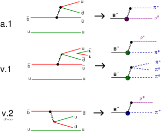
Figure 12: From quarks to hadronized Feynman diagrams contribution to $B^{+}\to\pi^{-}\pi^{+}\pi^{+}$ decay.

In addition to the tree diagram, the decay amplitude includes a contribution from re-scattering. By re-scattering, here, we mean the interaction between the pion produced from the vacuum with the one produced from the $\rho$- meson. Therefore, the amplitude for $B^{+}\to\pi^{-}\pi^{+}\pi^{+}$ decay is represented by the series of diagrams in Fig. 11.

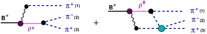
Figure 13: Diagrams contributing to $B^{+}\to\pi^{-}\pi^{+}\pi^{+}$ decay amplitude.

In this qualitative study, we focus on the role of the second diagram in Fig. 11 in the $B^{+}\to\pi^{-}\pi^{+}\pi^{+}$ decay amplitude. For this reason, the contribution from the weak vertex is not included, and this will be studied in the near future. It is important to note that neglecting this contribution will not affect the conclusions of this study, since both diagrams in Fig. 11 have the same weak vertex.

Tree amplitude - $A_{0}$

The tree level contribution to the $B^{+}\to\pi^{-}\pi^{+}\pi^{+}$ decay amplitude, the first diagram in Fig. 11, denoted here as $A_{0}$, is given by:

$$A_{0} = C_{0}\,[-p_{1}\,\cdot(p_{2}-p_{3})]\,F^{1}_{\pi\pi}(s_{23});$$ (74)

where $C_{0}$ is a constant and $F_{0}^{B\rho}(p_{1}^{2})$ is the form factor related to the $B\to\rho$ amplitude. The product $-p_{1}\,\cdot(p_{2}-p_{3})\equiv(s_{13}-s_{12})$ accounts for the angular distribution of the P-wave.

Production amplitude: $\rho\to\pi\pi$

The $\rho$ production amplitude is a crucial element in the description of the $B^{+}\to\pi^{-}\pi^{+}\pi^{+}$ decay for both tree and re-scattering amplitudes.

Figure 14: Diagrams for process $\rho\to\pi\pi$.

The corresponding amplitude of this process, shown in Fig. 12, can be expressed terms of the $\pi\pi$ scattering amplitude using the K-matrix approximation, as in Ref. Boito and Robilotta (2007),

$$F^{1}_{\pi\pi}(s)=G_{\rho}\frac{\cos\delta(s)}{m_{\rho}^{2}-s}\,e^{i\delta(s)}$$ (75)

where $\delta(s)$ is the $\pi\pi$ phase shift. In Eq. (75) we use the CERN-Munich parameterization Hyams et al. (1973); *cern-munich2 $\pi\pi$ phase shift, instead of using a model for the $\pi\pi$ scattering amplitude.

The production amplitude, Eq. (75), is inside the hadronic loop in the re-scattering calculation, therefore, the amplitude needs to be integrated with the loop. We parametrize the experimental data by a sum of poles with a complex constant in the numerator Magalhães and Robilotta (2015), and write

$$F^{1}_{\pi\pi}(s)=\sum_{i=1}^{3}\frac{N_{\rho i}}{s-\Theta_{i}}\,;$$ (76)

where the values of $N_{\rho i}$ and $\Theta_{i}=a+ib$ are available in table I of Ref. Magalhães and Robilotta (2015). The advantage of this form is to allow us to use Feynman rules to integrate the loop, as will become clear in the following.

Re-scattering amplitude - A1

The re-scattering contribution, second diagram in Fig. 11, can be written in terms of the tree amplitude as:

$$A_{1}=-i\int\frac{d^{4}\ell}{(2\pi)^{4}}\;\frac{T_{\pi\pi}\,A_{0}}{{D}_{\pi}^{+}\,{D}_{\pi}^{-}}\;,$$ (77)

where $T_{\pi\pi}$ is the $\pi\pi$ scattering amplitude represented by the green bubble and ${D}_{\pi}^{+}$, $\,{D}_{\pi}^{-}$ are the pion propagators inside the loop, ${D}_{\pi}^{+}=(P_{B}-l)^{2}-M^{2}_{\pi}$ and ${D}_{\pi}^{-}=(l-p_{3})^{2}-M^{2}_{\pi}$. It is important to note that the $B\to\rho$ form factor is not a constant any more because the transferred momentum is integrated over in the loop. In this case, we use a monopole approximation and

$$F_{0}^{B\rho}(p_{1}^{2})=-\frac{F_{B\rho}(0)\,m^{2}_{B*}}{\,{D}_{B*}};\,\,\,\,{D}_{B*}=(P_{B}-l)^{2}-m^{2}_{B*}\,.$$ (78)

Finally, the re-scattering amplitude for $B^{+}\to\pi^{-}\pi^{+}\pi^{+}$ is given by:

$$A_{1} = i\frac{C_{O}\,m^{2}_{B*}}{2\,}\,T^{P}_{\pi\pi}(s_{23})\,N_{\rho}\,\left\{\,I_{1}-I^{t}_{2}\,\,\right\},$$ (79)

where $I_{1}$ and $I^{t}_{2}$ are functions of scalar and tensorial loop integrals, respectively,

$$I_{1}=(s_{12}-s_{13})\, \frac{i}{16\pi^{2}} \,\left\{\left(M^{2}_{B}-\,2\,s_{23}+3\,M^{2}_{\pi}+\Theta_{i}\right)\Pi_{\pi^{+}\pi^{-}B^{*}\rho_{i}}+\Pi_{\pi^{-}B^{*}\rho_{i}}\right.$$ (80)

$$+\left.2\,\Pi_{\pi^{+}B^{*}\rho_{i}}-\,\Pi_{\pi^{+}\pi^{-}B*}\right\}\,,$$

$$I^{t}_{2}=2\,(p_{2}-p_{3})_{\mu}\, \frac{i}{16\pi^{2}} \,\left\{\left(M^{2}_{B}-\,2\,s_{23}+3\,M^{2}_{\pi}+\Theta_{i}\right)\Pi^{\mu}_{\pi^{+}\pi^{-}B*\rho_{i}}+\Pi^{\mu}_{\pi^{-}B^{*}\rho_{i}}\right.$$ (81)

$$+\left.2\,\Pi^{\mu}_{\pi^{+}B^{*}\rho_{i}}-\,\Pi^{\mu}_{\pi^{+}\pi^{-}B^{*}}\right\}\,,$$

and the indices on functions type $\Pi_{xyz}$ refer to the particles that are taking part in the loop. All these loop integrals can be solved using Feynman integral technique. A guide for all calculations can be find in Ref. Magalhães (2014).

XVI.3 Results

We compare numerically the individual contributions from the tree and re-scattering amplitudes to the total $B^{+}\to\pi^{-}\pi^{+}\pi^{+}$ amplitude.

In Fig. 13 individual contributions to the P-wave phase are shown as a function of the $\pi\pi$ invariant mass. Although they look similar, at threshold the re-scattering contribution, Eq. (79), starts below $-60^{o}$ and crosses $90^{o}$ in a different position than the tree contribution. Even if one shift up the re-scattering contribution, they have a clear different energy dependence on the lower sector.

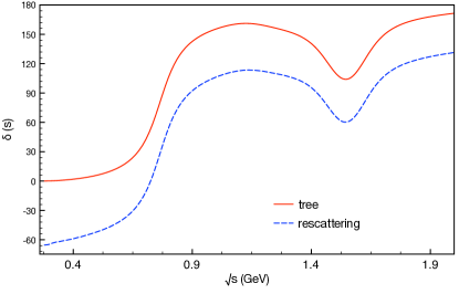
Figure 15: Amplitude phase for tree, Eq.(74), and re-scattering, Eq.(79), contributions.

In Fig. 14 we show the results for the modulus. In the plot on the left one can see that the two amplitudes interfere destructively with the dominance of the former. Is possible to note a presence of a smaller peak around $1.7$ GeV, which is the contribution of the $\rho(1450)$ coming from the $T_{\pi\pi}$ scattering amplitude. In the plot on the right, the two contributions are superimposed, with the re-scattering contribution rescaled. The two line shapes are very different. Not only is the position of the peak different, but also the two curves are asymmetric in opposite directions, with the re-scattering curve being wider than the curve from the tree amplitude.

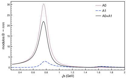
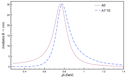
Figure 16: Magnitude square of the tree Eq.(74), re-scattering Eq.(79) and final amplitude. The plot on the right has the two contributions superimposed with a scale factor applied to the re-scattering curve.

Data analysis

Two samples of Toy Monte-Carlo with 10,000 events were generated to $B\to\rho\pi$ decays using the amplitude derived in the previous section. A first sample is generated with only the tree amplitude. A second sample is generated with the full amplitude, including the re-scattering contribution. The samples are then fitted with isobar model tools, such as Relativistic Breit-Wigner functions with no barriers factors. A good fit is obtained for the tree-only sample. This is expected, since the only ingredient is the $\rho$ production amplitude of Eq.(75). The results for the resonance parameters are: $m_{\rho}=0.775\pm 0.001$GeV, $\Gamma_{\rho}=0.148\pm 0.001$GeV, where the uncertainties are due to the sample size. Comparing to the PDGOlive et al. (2014b) values: $m_{\rho}=0.77526\pm 0.00025$ GeV and $\Gamma_{\rho}=0.1491\pm 0.0008$ GeV, one can see that they nicely agree.

When we add the re-scattering contribution to the tree one, defining the complete amplitude to $B^{+}\to\pi^{-}\pi^{+}\pi^{+}$ decay, there is a presence of a second bump in the amplitude due to the $\rho(1450)$ present on the re-scattering amplitude. Therefore the sample simulated with the full amplitude can be fitted by a sum of two Breit-Wigner functions, yielding the following parameters: $m_{\rho}=0.756\pm 0.001$GeV, $\Gamma_{\rho}=0.163\pm 0.003$GeV and $m_{\rho 2}=1.50\pm 0.01$GeV, $\Gamma_{\rho 2}=0.194\pm 0.033$GeV; where the uncertainties are statistical. The first $\rho$ contribution is the result of the tree and re-scattering interference and the second $\rho$ came only from the rescattering (Fig. 14, left). Comparing the results of the two fits, one can see that the inclusion of the re-scattering amplitude changes slightly the $\rho$ mass with a significant increase in the width. The re-scattering contribution to the amplitude, function $A_{1}$, is not fitted with two Breit-Wigner functions. However, we manage to parametrized this function using one Landau and two Gaussian functions, the result is shown in Fig. 15.

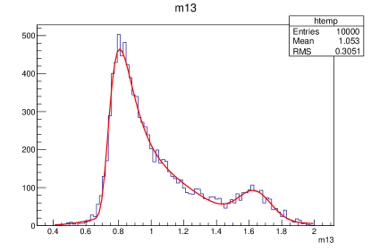
Figure 17: Fit to re-scattering amplitude, Eq.(79)

XVI.4 Final remarks

The inclusion of re-scattering introduce new complexities into the game, it shifts the phase at threshold to bellow zero and change the shape of the $\rho$ meson in the final amplitude. Inspecting the diagram in fig.12, we can conclude that these effect came from the hadronic loop. It is important to note that the $\rho$ meson we seeing in the Dalitz plot, or data, is an overlap of all $\rho$’s: the one produced directly from B decays and the one produced from the re-scattering. Therefore, we need to take this in the account when performing fits.

XVI.5 Acknowledgements

We would like to thank the workshop organizer for the pleasant environment and friendly reception. The work of PCM was supported by CNPq (Conselho Nacional de Desenvolvimento Científico e Tecnológico).

XVII Breit-Wigner, resonance propagator, scattering amplitudes, and production amplitudes: Who is who?

P. C. Magalhães^a and M.R. Robilotta^{b a}Centro Brasileiro de Pesquisas Físicas – CBPF
Rio de Janeiro, Brazil ^bInstituto de Física, Universidade de São Paulo,
São Paulo, Brazil

The LHCb workshop on amplitude analyses, held in CBPF, raised many interesting discussions. Among them, the role of Breit-Wigner functions embodied into two-body scattering amplitudes used in experimental analyses. It became clear that there is considerable confusion on this topic, associated mostly with the use of the name Breit-Wigner in different contexts. In this contribution, we aim to clarify this issue, by discussing the differences between resonance propagators, scattering amplitudes and production amplitudes involving resonances, emphasizing their connection with the different Breit-Wigner functions. This paper is a short version of a more detailed work to be presented in a near future.

XVII.1 Introduction

In their original 1936 paper, Breit and Wigner Breit and Wigner (1936) described the capture of slow neutrons by nuclei by means of cross sections, written generically as

$$\sigma=\alpha\;\frac{1}{(\nu-\nu_{0})^{2}+\Gamma^{2}}\;,$$ (82)

where $\alpha$ was a suitably chosen function of energy, $\nu$ and $\nu_{0}$ were energies, and $\Gamma$ was related with the half width breadth. As time went by, several other functions, sharing the same kind of denominator, became also known as Breit-Wigner functions (BW). As these various functions describe different objects, such as propagators, two-body scattering amplitudes or many-body production amplitudes, which occur in different situations, the result was a big mess of names and meanings.

As the denominators we are interested in originate from resonance propagators, we begin by sketching their main features and discuss their insertion into amplitudes afterwards. While doing this, it is useful to distinguish theory from models. As one is dealing with relativistic particles, the natural framework for the former is quantum field theory (QFT). Models, on the other hand, depart from theoretical results and introduce reasonable ad hoc modifications, aimed at improving their efficacy in describing data.

XVII.2 Propagators - theory

Bare propagator

This discussion is standard and can be found, for instance, in the book by Bjorken and Drell Bjorken and Drell (1964). In QFT, one is entitled to imagine a world in which a particle, such as the $\rho$-meson, lives in complete isolation. The propagator of this particle, ${D}_{0}\,$, can be derived from a Lagrangian involving its bare mass $m_{0}$, and is written as

$$i{D}_{0}(s) \!=\! i\,\frac{\Pi_{J}}{D_{0}(s)}\;,\hskip 28.45274ptD_{0}(s)\!=\!s-m_{0}^{2}\;,$$ (83)

where the numerator $\Pi_{J}$ is a projector, associated with the spin $J$. For instance, $J=0\rightarrow\Pi_{S}=1;J=1\rightarrow\Pi_{P}=g^{\mu\nu}-p^{\mu}p^{\nu}/m^{2}...$ . In this work, we concentrate just on denominators and do not care about numerators.

Dressed propagator

If the propagating particle can interact with two other particles, which we will call $A$ and $B$, its energy changes as does its mass. In the case of the $\rho$, the other two particles could be $[A\,B]\rightarrow[\gamma\,\rho],[\pi\;\pi],[K\,\bar{K}],[p\,\bar{p}],\cdots$, and systems involving more than two particles are also possible.

Figure 18: The dressing of a bare propagator.

The possibility of interactions means that the original propagating particle can transform itself into particles $A$ and $B$ which, in turn, can yield back the propagating particle. In the case of the $\rho$, one could have $\rho\rightarrow\pi\,\pi$ and, afterwards $\pi\,\pi\rightarrow\rho$. This yields a characteristic self-energy, usually denoted by $\Sigma$, which, by means of the geometric series indicated in eq. (84) and Fig. 18, give rise to the dressed propagator ${D}$,

$$i{D}=i{D}_{0}+i{D}_{0}\,\left[-i\,\Sigma\,\right]\,i{D}_{0}+i{D}_{0}\,\left[-i\,\Sigma\,\right]\,i{D}_{0}\,\left[-i\,\Sigma\,\right]\,i{D}_{0}\,+\cdots\;,$$ (84)

This sum can be expressed in a more compact form as

$$i{D}(s) \!=\! i\,\frac{\Pi_{J}}{D(s)}\;,\hskip 28.45274ptD(s)\!=\!s-m_{0}^{2}-\Sigma(s)\;.$$ (85)

The important feature to be noted is that the availability of different intermediate states for the propagating particle modifies the function $D(s)$. This denominator is a Lorentz scalar so as the function $\Sigma$. This result is model independent and specific choices of the function $\Sigma$ eventually yield a BW functions.

In QFT, the function $\Sigma$ is formally associated with two effects, namely the wave function renormalization $Z$ and the modification of the particle mass. These features are formally introduced by noting that the physical mass $m$ is fixed as the solution of the equation

$$m_{0}^{2}+\Sigma(m^{2})=m^{2}\;.$$ (86)

After fixing $m$, one expands the self-energy as Scherer (2003)

$$\Sigma(s)=\Sigma(m^{2})+(s-m^{2})\,\Sigma^{\prime}(m^{2})+\tilde{\Sigma}(s)\;,$$ (87)

and rewrites the denominator as

$$D(s)=\left[1-\Sigma^{\prime}(m^{2})\right]\left[(s-m^{2})-\frac{\tilde{\Sigma}(s)}{1-\Sigma^{\prime}(m^{2})}\right]\;.$$ (88)

The first factor in this result is absorbed into a redefinition of the fields and the renormalized propagator, indicated by a bar, is given by

$$i\bar{{D}}(s) \!=\! i\,\frac{\Pi_{J}}{\bar{D}(s)}\;,\hskip 28.45274pt\bar{D}(s)\!=\!s-m^{2}-\frac{\tilde{\Sigma}(s)}{1-\Sigma^{\prime}(m^{2})}\;.$$ (89)

If the only effect of the self-energy were the shift in the mass, the denominator $D(s)$ would have a simple pole at $s=m^{2}$. However, the term proportional to $\tilde{\Sigma}(s)$ cannot be neglected and may give rise to important consequences, such as bound states or resonance widths.

The self-energy $\Sigma$

The properties of the self-energy $\Sigma$ can be discussed in general terms and one finds that:
- $\Sigma$ can be either a real function or a complex function, depending on how the mass of the propagating particle relates with the masses present in the intermediate system.
- the form of $\Sigma$ depends on the angular momentum of the propagating particle.

As the general discussion is well beyond our limited scope, here we introduce these features by means of specific examples.

Scalar resonances

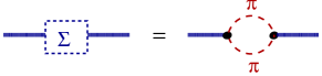
Figure 19: The self-energy mechanism.

In the case of a scalar resonance, such as the $f_{0}$, which can decay into two pions, the expression for the self energy involves twice the factor $G_{S}$, associated with the transitions $f_{0}\rightarrow\pi\pi$ and $\pi\pi\rightarrow f_{0}$, together with the two-pion propagator. The important point is that $G_{S}$ is a real function and the scalar self-energy reads

$$\Sigma_{S}=G_{S}\,\bar{\Omega}_{S}\,G_{S}\;,$$ (90)

where $\bar{\Omega}_{S}$ is a function related with the two-pion propagator and written as

$$\Omega_{S}(s) \!=\! i\,\int\frac{d^{4}\ell}{(2\pi)^{4}}\;\frac{1}{[(\ell\!+\!p/2)^{2}-M_{\pi}^{2}+i\,\epsilon\,]\;[(\ell\!-\!p/2)^{2}-M_{\pi}^{2}+i\,\epsilon\,]}\;,$$ (91)

with $p^{2}=s$. This integral is divergent and the strategy for dealing with this unwanted feature is to write $\Omega_{S}(s)=\bar{\Omega}_{S}(s)+\Omega_{S}(0)$, where $\bar{\Omega}_{S}(s)$ is a regular function and the divergence is kept in $\Omega_{S}(0)$. The integral is then regularized and the net effect is the replacement $\Omega_{S}(0)\rightarrow C$, where $C$ is a finite but unknown constant, which must be fixed by data. The regular part $\bar{\Omega}_{S}(s)$, can be evaluated explicitly along different intervals of the variable $\lambda^{2}=(s-4M_{\pi}^{2})/s$ and one has

$$s\!<\!0 \rightarrow \bar{\Omega}_{S}=-\,\frac{1}{32\pi^{2}}\,\left[2-2\;\frac{\sqrt{|s|\!+\!4M_{\pi}^{2}}}{\sqrt{|s|}}\,\ln\frac{\sqrt{|s|+4M_{\pi}^{2}}+\sqrt{|s|}}{2\,M_{\pi}}\right]\;,$$ (92)

$$0\!\leq\!s\!<\!4\,M_{\pi}^{2} \rightarrow \bar{\Omega}_{S}=-\,\frac{1}{32\pi^{2}}\,\left[2-\;2\,\frac{\sqrt{4M_{\pi}^{2}-s}}{\sqrt{s}}\;\tan^{-1}\left(\frac{\sqrt{s}}{\sqrt{4M_{\pi}^{2}-s}}\right)\right]\;,$$ (93)

$$s\!\geq 4\,M_{\pi}^{2} \rightarrow \bar{\Omega}_{S}=-\,\frac{1}{32\pi^{2}}\,\left[2-2\,\frac{\sqrt{s-4M_{\pi}^{2}}}{\sqrt{s}}\;\ln\frac{\sqrt{s-4M_{\pi}^{2}}+\sqrt{s}}{2\,M_{\pi}}+\,i\,\pi\;\frac{\sqrt{s-4M_{\pi}^{2}}}{\sqrt{s}}\;\right]\;.$$ (94)

On quite general grounds, the imaginary part of a self-energy can be associated with $\tau^{-1}$, where $\tau$ is the proper lifetime of the propagating particle Brown (1994) . In the present example, the resonance can decay only when $s\geq 4\,M_{\pi}^{2}$ and this is the reason why only Eq.(94) contains an imaginary component. This idea can be reinforced by recalling that the very concept of lifetime does not apply to virtual states.

Assembling all these pieces into Eq.(87) one obtains the self-energy for a scalar resonance, where the numerical value for $\Sigma^{\prime}(m^{2})$ is small and the factor $\frac{1}{1-\Sigma^{\prime}(m^{2})}$ can be set to one in Eq(88). Then, the renormalized resonance propagator, Eq.(89), becomes

$$D_{S}(s)=s-{\cal{M}}_{S}^{2}(s)+\,i\;\Theta(s-4M_{\pi}^{2})\;G_{S}^{2}\,\frac{\sqrt{s-4M_{\pi}^{2}}}{32\pi\,\sqrt{s}}$$ (95)

where

$${\cal{M}}_{S}^{2}(s)=m_{0}^{2}+G_{S}^{2}\,\left\{\left[\bar{\Omega}_{S}\right]_{R}+C\right\}\;$$ (96)

is the running mass. The physical mass $m_{S}$ of the resonance is the solution of the equation ${\cal{M}}_{S}^{2}(s=m_{S}^{2})=m_{S}^{2}\;.$ Once the value of $m$ is fixed, the resonance propagator is conventionally written as

$$i{D}_{S}(s)=\frac{i}{D_{S}(s)}\;,\hskip 28.45274ptD_{S}(s)=s-{\cal{M}}_{S}^{2}(s)+\,i\;\Theta(s-4M_{\pi}^{2})\;m_{S}\;\Gamma_{S}(s)\;,$$ (97)

$$\Gamma_{S}(s)=\frac{G_{S}^{2}}{32\pi\,m_{S}}\;\frac{\sqrt{s-4M_{\pi}^{2}}}{\sqrt{s}}\;.$$ (98)

Comparing the final expression for the propagator in Eq.(97) with the one derived from QFT, Eq.(89), one can see the relevance of the factor $\tilde{\Sigma}(s)$ for the width, Eq.(98), and the running mass, Eq.(96). This final form of the propagator also indicates that the expressions that look like BWs arise naturally in the framework of QFT.

One notes that the functions $D(s)$, ${\cal{M}}(s)$ and $\Gamma(s)$ entering the propagator are Lorentz scalars and the width is linear in $q$, the three-momentum of the intermediate pions in their CM.

Vector resonances

As discussed above, the bare propagator of a vector resonance involves a characteristic numerator. In the dressing process, this factor also influences the self-energy $\Sigma_{P}$ and, therefore, the denominator. The net effect corresponds to the inclusion of an extra kinematic factor.

$$\bar{\Omega}_{S}\rightarrow\bar{\Omega}_{P}=\frac{1}{3}\,[s\!-\!4\,M_{\pi}^{2}]\;\bar{\Omega}_{S}\;,$$ (99)

and this leads us to

$$i{D}_{P}(s)=\frac{i}{D_{P}(s)}\;,\hskip 28.45274ptD_{P}(s)=s-{\cal{M}}_{P}^{2}(s)+\,i\;\Theta(s-4M_{\pi}^{2})\;m_{P}\;\Gamma_{P}(s)\;,$$ (100)

$${\cal{M}}_{P}^{2}(s)=m_{0}^{2}+G_{P}^{2}\,\left[\bar{\Omega}_{P}+C_{P}\,\right]\;,\hskip 22.76219pt\Gamma_{P}(s)=\frac{G_{P}^{2}}{96\pi\,m_{P}}\;\frac{[s\!-\!4\,M_{\pi}^{2}]\,\sqrt{s\!-\!4M_{\pi}^{2}}}{\sqrt{s}}\;.$$ (101)

In the rest frame of the vector resonance, the width is proportional to $q^{3}$. Once again, the vector resonance propagator shows that the contribution from $\tilde{\Sigma}(s)$ to the self-energy, eq.(87), is very significant to both the resonance width and running mass. It is very interesting to point-out that the expression to the vector propagator, Eq.(100), is the same as the one proposed by Gounaris-SakuraiGounaris and Sakurai (1968) as we show below, in Eq.(106).

Poles

Poles of propagators are important and can be determined from denominators such as those given by eqs. (97) and (100). Schematically, they are obtained by writing $s=(a-i\,b)^{2}$ and then determining the values of $a$ and $b$ by means of the condition

$$D_{J}[(a-i\,b)^{2}]=0.$$ (102)

Calling $a=m_{pole}$ and $b=\Gamma_{pole}/2$, one finds representations for the propagator of the form

$$i\,{D}_{J}(s)=\frac{\mathrm{residue}}{s-(m_{J\,pole}-i\,\Gamma_{J\,pole}/2)^{2}}+\mathrm{non\!-\!pole}\;.$$ (103)

One notes that:
- The values of $m_{J\,pole}$ and $\Gamma_{J\,pole}$ need not to be close to the values of $m_{J}$ and $\Gamma_{J}$ in eqs.(97) and (100).
- There may exist more than one solution to eq. (102), representing dynamically generated states.

XVII.3 Models

The description of systems involving resonances may become cumbersome in QFT, when several different degrees of freedom are involved. In this case, it is usual that results from QFT are extended by means of ad hoc modifications, based on educated guesses. Some popular choices for the case of the $\rho$-meson are presented below.

$K$-matrix

In the so-called $K$-matrix approximation, the running masses ${\cal{M}}^{2}(s)$ in eqs. (97) and (100) are replaced with the fixed empirical resonance masses, and one employs denominators of the form.

$$D_{J}(s)=s-m_{J}^{2}+\,i\;\Theta(s-4M_{\pi}^{2})\;m_{J}\;\Gamma_{J}(s)\;.$$ (104)

This expression is the same as that used in the isobar model without barriers factors.

Gounaris-Sakurai

The form of the propagator known as Gounaris-Sakurai (GS) was developed in 1968 Gounaris and Sakurai (1968) and expresses the physics just described. Using their notation, we have

$$i{D}_{GS}(s) \!=\! \frac{i}{D_{GS}(s)}\,,\hskip 28.45274ptD_{GS}(s)\!=\!s-[m_{\rho}^{2}+f(s)]+im_{\rho}\Gamma(s)\,,$$ (106)

$$\Gamma(s)=\Gamma_{\rho}\;\frac{m_{\rho}}{\sqrt{s}}\;\left[\frac{k(s)}{k(m_{\rho}^{2})}\right]^{3}\,;\hskip 28.45274ptk(s)=\sqrt{\frac{s-4M_{\pi}^{2}}{4}}\,;$$

$$f(s) = \Gamma_{\rho}\;\frac{m_{\rho}^{2}}{k(m_{\rho}^{2})^{3}}\;\left[k(s)^{2}\,\left(h(s)-h(m_{\rho}^{2})\right)+(m_{\rho}^{2}-s)\,h^{\prime}\,k(m_{\rho}^{2})^{2}\right]\,;$$ (108)

$$h(s)=\frac{2}{\pi}\,\frac{k(s)}{\sqrt{s}}\;\ln\left[\frac{\sqrt{s}+2k(s)}{2M_{\pi}}\right]\,;\hskip 22.76219pth^{\prime}=h(m_{\rho}^{2})\;\left[\frac{1}{8k(m_{\rho}^{2})^{2}}-\frac{1}{2m_{\rho}^{2}}\right]+\frac{1}{2\pi m_{\rho}^{2}}.$$

The Gounaris-Sakurai expression for the width is identical to that of eq. (101), provided one defines $\Gamma_{\rho}=\Gamma(s=m_{\rho}^{2})$ and then uses this to replace the factor $G_{P}^{2}/(96\pi\,m_{\rho})$ present there. Eq. (97) yieds $h(s)=16\pi\,\bar{\Omega}_{S}-1/\pi$ and the function $f(s)$ amounts to the expansion of the real part of the self-enegy around $s=m_{\rho}^{2}$, given by eq. (87).

Isobar model

In the isobar model the following expression is widely used in fits to data

$$i{D}_{IM}^{\rho}(p) \!=\! \frac{i}{s-m_{\rho}^{2}+im_{\rho}\,\Gamma_{\rho}^{IM}(s)}\;,\hskip 28.45274pt\Gamma_{\rho}^{IM}(p)=\Gamma_{\rho}^{GS}\left[\frac{F_{r}(s)}{F_{r}(m_{\rho}^{2})}\right]^{2}\;,$$ (109)

where $\Gamma_{\rho}^{GS}$ is given by eq.(106) and $F_{r}(s)=1/\sqrt{1+[r_{r}q_{r}(s)]^{2}}$. This function becomes identical to the K-Matrix, eq. (104), if we take out the barrier factors.

XVII.4 Scattering amplitudes

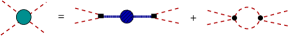
Figure 20: $\pi\pi$ scattering amplitude: resonances exchange and meson-meson interaction.

Scattering amplitudes are the usual sources of resonance information. However, scattering amplitudes may receive contributions from many kinds of processes, not all of them associated with resonances, as in Fig. 20. This gives rise to important differences between denominators entering propagators and amplitudes. We discuss this feature by means of an example concerning the $P$-wave $\pi\pi$ elastic amplitude. One assumes a simple $\pi\pi$ interaction, based on just an $s$-channel $\rho$-pole and a background $B$, as in Fig. 20.

Using a chiral model Magalhães and Robilotta (2015) as a guide, the construction of the amplitude begins by describing the tree diagrams, which yield

$$\bar{T^{1}}=(t-u)\left[B-G_{\rho}^{2}\,\frac{s}{s-m_{\rho}^{2}}\right]\,,$$ (110)

where $s$, $t$ and $u$ are the Mandelstam variables and $B=1/F^{2}$. For free particles in the center of mass frame, $(t-u)=(s-4M_{\pi}^{2})\,\cos\,\theta$ and the $P$-wave projection gives rise to the kernel

$${\cal{K}}^{P1} = -\,\frac{(s-4M_{\pi}^{2})}{3\,}\;\left[B+G_{\rho}^{2}\frac{s}{s-m_{\rho}^{2}}\right]=-\,\frac{(s-4M_{\pi}^{2})}{3\,}\;\left[\frac{B(s-m_{\rho}^{2})+G_{\rho}^{2}\,s}{s-m_{\rho}^{2}}\right]$$ (111)

which can be used to construct a unitarized scattering amplitude Oller and Oset (1999), given by

$$T_{\pi\pi}^{P1}=\frac{{\cal{K}}^{P1}}{1+{\cal{K}}^{P1}\,(\bar{\Omega}_{\pi\pi}+C_{\pi\pi})}\;=\frac{\,(4M_{\pi}^{2}-s)/3\;\left[B(s-m_{\rho}^{2})+G_{\rho}^{2}\,s\right]}{s-m_{\rho}^{2}-\left[B(s-m_{\rho}^{2})+G_{\rho}^{2}\,s\right]\,(\bar{\Omega}_{P}+C_{P})}\;.$$ (112)

This gives rise to a denominator which is different from all the previous ones discussed and, in particular, to a width of the form

$$\Gamma_{\rho}^{T}(s)=\frac{\left[B(s-m_{\rho}^{2})+G_{\rho}^{2}\,s\right]}{96\pi}\;\frac{[s\!-\!4\,M_{\pi}^{2}]\,\sqrt{s\!-\!4M_{\pi}^{2}}}{\sqrt{s}}\;.$$ (113)

The presence of the background $B$ in this result is a clear indication that it does influence the width profile for $s\neq m_{\rho}^{2}$.

XVII.5 Production amplitude: $\rho^{0}\to\pi^{+}\pi^{-}$

The $\rho$ meson can be produced directly in B or D decays before it decays into two mesons. The same model used to derive the scattering amplitude, eq. (112), yields the production amplitude

$$\Pi(s) = A\;\frac{G_{\rho}}{m_{\rho}^{2}-s}\left[1+(-\bar{\Omega})\frac{{\cal{K}}}{1+\bar{\Omega}{\cal{K}}}\right]=A\;\frac{G_{\rho}}{m_{\rho}^{2}-s}\left[\frac{1}{1+\bar{\Omega}{\cal{K}}}\right]$$ (114)

$$= A\;\frac{G_{\rho}}{m_{\rho}^{2}-s+\left[B(s-m_{\rho}^{2})+G_{\rho}^{2}\,s\right]\,(\bar{\Omega}_{P}+C_{P})}.$$ (115)

where $A$ is a factor describing the transition of the heavy mesons into $\rho+$other mesons. Comparing eq. (115) with the resonance propagator, eq. (100), one can see that, again, both the width and the running mass are different due to the presence of a background in the kernel.

XVII.6 Final remarks

We inspect the general ground of the structures used to describe resonance propagators in different context. It became clear that the functional form of the resonance propagation depend strongly on the environment and the dynamical model considered. We show that availability of different intermediate states can give an important contributions and change both the mass and the width of the resonances propagator. This difference is also manifest on the extraction of the pole position, once the source propagation is not universal so as the associated pole position.

XVII.7 Acknowledgements

We would like to thank the workshop organizer for the pleasant environment and friendly reception. The work of PCM was supported by CNPq (Conselho Nacional de Desenvolvimento Científico e Tecnológico).

References

- Aaij et al. (2014a) R. Aaij et al. (LHCb collaboration), Phys. Rev. D90, 072003 (2014a), arXiv:1407.7712 [hep-ex] .
- Aaij et al. (2015a) R. Aaij et al. (LHCb collaboration), Phys. Rev. D91, 092002 (2015a), arXiv:1503.02995 [hep-ex] .
- Aaij et al. (2015b) R. Aaij et al. (LHCb collaboration), Phys. Rev. D92, 032002 (2015b), arXiv:1505.01710 [hep-ex] .
- Aaij et al. (2015c) R. Aaij et al. (LHCb collaboration), Phys. Rev. D92, 012012 (2015c), arXiv:1505.01505 [hep-ex] .
- Gershon (2009) T. Gershon, Phys. Rev. D79, 051301 (2009), arXiv:0810.2706 [hep-ph] .
- Gershon and Williams (2009) T. Gershon and M. Williams, Phys. Rev. D80, 092002 (2009), arXiv:0909.1495 [hep-ph] .
- Latham and Gershon (2009) T. Latham and T. Gershon, J. Phys. G36, 025006 (2009), arXiv:0809.0872 [hep-ph] .
- Charles et al. (1998) J. Charles, A. Le Yaouanc, L. Oliver, O. Pene, and J. C. Raynal, Phys. Lett. B425, 375 (1998), [Erratum: Phys. Lett.B433,441(1998)], arXiv:hep-ph/9801363 [hep-ph] .
- Bugg (2009) D. V. Bugg, J. Phys. G36, 075003 (2009), arXiv:0901.2217 [hep-ph] .
- Veneziano (1968) G. Veneziano, Nuovo Cim. A57, 190 (1968).
- Aaij et al. (2014b) R. Aaij et al. (LHCb collaboration), Phys. Rev. D90, 112004 (2014b), arXiv:1408.5373 [hep-ex] .
- Aubert et al. (2008a) B. Aubert et al. (BaBar), Phys. Rev. D78, 051102 (2008a), arXiv:0802.4035 [hep-ex] .
- Bediaga et al. (2009) I. Bediaga, I. I. Bigi, A. Gomes, G. Guerrer, J. Miranda, and A. C. d. Reis, Phys. Rev. D80, 096006 (2009), arXiv:0905.4233 [hep-ph] .
- Bediaga et al. (2012) I. Bediaga, J. Miranda, A. C. dos Reis, I. I. Bigi, A. Gomes, J. M. Otalora Goicochea, and A. Veiga, Phys. Rev. D86, 036005 (2012), arXiv:1205.3036 [hep-ph] .
- Bediaga et al. (2014) I. Bediaga, T. Frederico, and O. Louren o, Phys. Rev. D89, 094013 (2014), arXiv:1307.8164 [hep-ph] .
- Alvarenga Nogueira et al. (2015) J. H. Alvarenga Nogueira, I. Bediaga, A. B. R. Cavalcante, T. Frederico, and O. Louren o, Phys. Rev. D92, 054010 (2015), arXiv:1506.08332 [hep-ph] .
- Magalhães et al. (2011) P. C. Magalhães, M. R. Robilotta, K. S. F. F. Guimarães, T. Frederico, W. de Paula, I. Bediaga, A. C. d. Reis, C. M. Maekawa, and G. R. S. Zarnauskas, Phys. Rev. D84, 094001 (2011), arXiv:1105.5120 [hep-ph] .
- Guimarães et al. (2014) K. S. F. F. Guimarães, O. Louren o, W. de Paula, T. Frederico, and A. C. dos Reis, JHEP 08, 135 (2014), arXiv:1404.3797 [hep-ph] .
- Frederico et al. (2014) T. Frederico, K. S. F. F. Guimarães, O. Lourenço, W. de Paula, I. Bediaga, and A. C. dos Reis, Proceedings, Venturing off the lightcone - local versus global features (Light Cone 2013), Few Body Syst. 55, 441 (2014), arXiv:1402.6975 [hep-ph] .
- Aitala et al. (2002) E. M. Aitala et al. (E791), Phys. Rev. Lett. 89, 121801 (2002), arXiv:hep-ex/0204018 [hep-ex] .
- Aitala et al. (2001a) E. M. Aitala et al. (E791), Phys. Rev. Lett. 86, 770 (2001a), arXiv:hep-ex/0007028 [hep-ex] .
- Aitala et al. (2001b) E. M. Aitala et al. (E791), Phys. Rev. Lett. 86, 765 (2001b), arXiv:hep-ex/0007027 [hep-ex] .
- Bonvicini et al. (2007) G. Bonvicini et al. (CLEO), Phys. Rev. D76, 012001 (2007), arXiv:0704.3954 [hep-ex] .
- Asner (2003) D. Asner, (2003), arXiv:hep-ex/0410014 [hep-ex] .
- Link et al. (2004) J. M. Link et al. (FOCUS), Phys. Lett. B585, 200 (2004), arXiv:hep-ex/0312040 [hep-ex] .
- Anisovich and Sarantsev (2003) V. V. Anisovich and A. V. Sarantsev, Eur. Phys. J. A16, 229 (2003), arXiv:hep-ph/0204328 [hep-ph] .
- Aitala et al. (2006) E. M. Aitala et al. (E791), Phys. Rev. D73, 032004 (2006), [Erratum: Phys. Rev.D74,059901(2006)], arXiv:hep-ex/0507099 [hep-ex] .
- Aubert et al. (2009a) B. Aubert et al. (BaBar), Proceedings, 34th International Conference on High Energy Physics (ICHEP 2008), Phys. Rev. D79, 032003 (2009a), arXiv:0808.0971 [hep-ex] .
- Hyams et al. (1973) B. Hyams et al., Nucl. Phys. B64, 134 (1973).
- Grayer et al. (1974) G. Grayer et al., Nucl. Phys. B75, 189 (1974).
- Link et al. (2009) J. M. Link et al. (FOCUS), Phys. Lett. B681, 14 (2009), arXiv:0905.4846 [hep-ex] .
- Aston et al. (1988a) D. Aston et al., Nucl. Phys. B296, 493 (1988a).
- Watson (1952) K. M. Watson, Phys. Rev. 88, 1163 (1952).
- Magalhães and Robilotta (2015) P. C. Magalhães and M. R. Robilotta, Phys. Rev. D92, 094005 (2015), arXiv:1504.06346 [hep-ph] .
- Achasov et al. (1979) N. N. Achasov, S. A. Devyanin, and G. N. Shestakov, Phys. Lett. B88, 367 (1979).
- Aaij et al. (2014c) R. Aaij et al. (LHCb collaboration), Phys. Rev. D90, 012003 (2014c), arXiv:1404.5673 [hep-ex] .
- Aaij et al. (2013a) R. Aaij et al. (LHCb collaboration), Phys. Rev. Lett. 110, 222001 (2013a), arXiv:1302.6269 [hep-ex] .
- Aaij et al. (2015d) R. Aaij et al. (LHCb collaboration), Phys. Rev. D92, 011102(R) (2015d), arXiv:1504.06339 [hep-ex] .
- Bugg (2008) D. V. Bugg, J. Phys. G35, 075005 (2008), arXiv:0802.0934 [hep-ph] .
- Esposito et al. (2014) A. Esposito, A. L. Guerrieri, F. Piccinini, A. Pilloni, and A. D. Polosa, Int. J. Mod. Phys. A30, 1530002 (2014), arXiv:1411.5997 [hep-ph] .
- Aaij et al. (2014d) R. Aaij et al. (LHCb collaboration), Phys.Rev.Lett. 112, 222002 (2014d), arXiv:1404.1903 [hep-ex] .
- Choi et al. (2008) S. Choi et al. (Belle collaboration), Phys.Rev.Lett. 100, 142001 (2008), arXiv:0708.1790 [hep-ex] .
- Aubert et al. (2009b) B. Aubert et al. (BaBar collaboration), Phys.Rev. D79, 112001 (2009b), arXiv:0811.0564 [hep-ex] .
- Chilikin et al. (2013) K. Chilikin et al. (Belle collaboration), Phys.Rev. D88, 074026 (2013), arXiv:1306.4894 [hep-ex] .
- Pakhlov and Uglov (2015) P. Pakhlov and T. Uglov, Phys. Lett. B748, 183 (2015), arXiv:1408.5295 [hep-ph] .
- Aaij et al. (2015e) R. Aaij et al. (LHCb), Phys. Rev. Lett. 115, 072001 (2015e), arXiv:1507.03414 [hep-ex] .
- Maiani et al. (2015) L. Maiani, A. D. Polosa, and V. Riquer, Phys. Lett. B749, 289 (2015), arXiv:1507.04980 [hep-ph] .
- Lebed (2015) R. F. Lebed, Phys. Lett. B749, 454 (2015), arXiv:1507.05867 [hep-ph] .
- Anisovich et al. (2015) V. V. Anisovich, M. A. Matveev, J. Nyiri, A. V. Sarantsev, and A. N. Semenova, (2015), arXiv:1507.07652 [hep-ph] .
- Karliner and Rosner (2015) M. Karliner and J. L. Rosner, Phys. Rev. Lett. 115, 122001 (2015), arXiv:1506.06386 [hep-ph] .
- Chen et al. (2015) R. Chen, X. Liu, X.-Q. Li, and S.-L. Zhu, Phys. Rev. Lett. 115, 132002 (2015), arXiv:1507.03704 [hep-ph] .
- Roca et al. (2015) L. Roca, J. Nieves, and E. Oset, (2015), arXiv:1507.04249 [hep-ph] .
- He (2015) J. He, (2015), arXiv:1507.05200 [hep-ph] .
- Meißner and Oller (2015) U.-G. Meißner and J. A. Oller, (2015), arXiv:1507.07478 [hep-ph] .
- Guo et al. (2015) F.-K. Guo, U.-G. Meißner, W. Wang, and Z. Yang, Phys. Rev. D92, 071502 (2015), arXiv:1507.04950 [hep-ph] .
- Liu et al. (2015) X.-H. Liu, Q. Wang, and Q. Zhao, (2015), arXiv:1507.05359 [hep-ph] .
- Mikhasenko (2015) M. Mikhasenko, (2015), arXiv:1507.06552 [hep-ph] .
- Szczepaniak (2015a) A. P. Szczepaniak, (2015a), arXiv:1510.01789 [hep-ph] .
- Aaij et al. (2014e) R. Aaij et al. (LHCb collaboration), Phys. Rev. Lett. 113, 162001 (2014e), arXiv:1407.7574 [hep-ex] .
- Aaij et al. (2015f) R. Aaij et al. (LHCb), (2015f), arXiv:1510.01951 [hep-ex] .
- Coffman et al. (1992) D. Coffman et al. (Mark III), Phys. Rev. D 45, 2196 (1992).
- Link et al. (2005a) J. M. Link et al. (FOCUS), Phys. Lett. B610, 225 (2005a), arXiv:hep-ex/0411031 [hep-ex] .
- Link et al. (2007) J. M. Link et al. (FOCUS), Phys. Rev. D75, 052003 (2007), arXiv:hep-ex/0701001 [hep-ex] .
- Link et al. (2003) J. M. Link et al. (FOCUS), Phys. Lett. B575, 190 (2003), arXiv:hep-ex/0308054 [hep-ex] .
- Artuso et al. (2012) M. Artuso et al. (CLEO collaboration), Phys. Rev. D85, 122002 (2012), arXiv:1201.5716 [hep-ex] .
- Gronau and Wyler (1991) M. Gronau and D. Wyler, Phys.Lett. B265, 172 (1991).
- Gronau and London (1991) M. Gronau and D. London, Phys.Lett. B253, 483 (1991).
- Atwood et al. (1997) D. Atwood, I. Dunietz, and A. Soni, Phys.Rev.Lett. 78, 3257 (1997), arXiv:hep-ph/9612433 [hep-ph] .
- Giri et al. (2003) A. Giri, Y. Grossman, A. Soffer, and J. Zupan, Phys. Rev. D 68, 054018 (2003).
- Poluektov et al. (2004a) A. Poluektov et al. (Belle), Phys. Rev. D 70, 072003 (2004a).
- Aubert et al. (2005) B. Aubert et al. (BaBar), Phys. Rev. Lett. 95, 121802 (2005), arXiv:hep-ex/0504039 [hep-ex] .
- Aubert et al. (2008b) B. Aubert et al. (BaBar), Phys. Rev. D78, 034023 (2008b), arXiv:0804.2089 [hep-ex] .
- Poluektov et al. (2004b) A. Poluektov et al. (Belle), Phys. Rev. D70, 072003 (2004b), arXiv:hep-ex/0406067 [hep-ex] .
- Poluektov et al. (2006) A. Poluektov et al. (Belle), Phys. Rev. D73, 112009 (2006), arXiv:hep-ex/0604054 [hep-ex] .
- Aaij et al. (2014f) R. Aaij et al. (LHCb collaboration), Nucl. Phys. B888, 169 (2014f), arXiv:1407.6211 [hep-ex] .
- Rademacker and Wilkinson (2007) J. Rademacker and G. Wilkinson, Phys.Lett. B647, 400 (2007), arXiv:hep-ph/0611272 [hep-ph] .
- Atwood and Soni (2003) D. Atwood and A. Soni, Phys. Rev. D68, 033003 (2003).
- Bondar and Poluektov (2006) A. Bondar and A. Poluektov, Eur. Phys. J. C47, 347 (2006), arXiv:hep-ph/0510246 [hep-ph] .
- Harnew and Rademacker (2014) S. Harnew and J. Rademacker, Phys.Lett. B728, 296 (2014), arXiv:1309.0134 [hep-ph] .
- Harnew and Rademacker (2015) S. Harnew and J. Rademacker, JHEP 03, 169 (2015), arXiv:1412.7254 [hep-ph] .
- Bondar and Poluektov (2007) A. Bondar and A. Poluektov, (2007), arXiv:hep-ph/0703267 [HEP-PH] .
- Bondar et al. (2010) A. Bondar, A. Poluektov, and V. Vorobiev, Phys.Rev. D82, 034033 (2010), arXiv:1004.2350 [hep-ph] .
- Malde and Wilkinson (2011) S. Malde and G. Wilkinson, Phys.Lett. B701, 353 (2011), arXiv:1104.2731 [hep-ph] .
- Aaij et al. (2015g) R. Aaij et al. (LHCb collaboration), (2015g), to appear in JHEP, arXiv:1510.01664 [hep-ex] .
- Briere et al. (2009) R. A. Briere et al. (CLEO), Phys.Rev. D80, 032002 (2009), arXiv:0903.1681 [hep-ex] .
- Insler et al. (2012) J. Insler et al. (CLEO), Phys.Rev. D85, 092016 (2012), arXiv:1203.3804 [hep-ex] .
- Libby et al. (2010) J. Libby et al. (CLEO), Phys.Rev. D82, 112006 (2010), arXiv:1010.2817 [hep-ex] .
- Lowrey et al. (2009) N. Lowrey et al. (CLEO), Phys.Rev. D80, 031105 (2009), arXiv:0903.4853 [hep-ex] .
- Libby et al. (2014) J. Libby, S. Malde, A. Powell, G. Wilkinson, D. Asner, et al., Phys.Lett. B731, 197 (2014), arXiv:1401.1904 [hep-ex] .
- Evans et al. (2016) T. Evans, S. Harnew, J. Libby, S. Malde, J. Rademacker, and G. Wilkinson, (2016), arXiv:1602.07430 [hep-ex] .
- Malde et al. (2015) S. Malde, C. Thomas, G. Wilkinson, P. Naik, C. Prouve, J. Rademacker, J. Libby, M. Nayak, T. Gershon, and R. A. Briere, Phys. Lett. B747, 9 (2015), arXiv:1504.05878 [hep-ex] .
- Nayak et al. (2015) M. Nayak, J. Libby, S. Malde, C. Thomas, G. Wilkinson, R. A. Briere, P. Naik, T. Gershon, and G. Bonvicini, Phys. Lett. B740, 1 (2015), arXiv:1410.3964 [hep-ex] .
- Lees et al. (2011a) J. Lees et al. (BaBar), Phys.Rev. D84, 012002 (2011a), arXiv:1104.4472 [hep-ex] .
- Adachi et al. (2011) I. Adachi et al. (Belle), (2011), arXiv:1106.4046 [hep-ex] .
- Aaij et al. (2012) R. Aaij et al. (LHCb), Phys. Lett. B718, 43 (2012), arXiv:1209.5869 [hep-ex] .
- Aaij et al. (2013b) R. Aaij et al. (LHCb), Phys.Lett. B726, 151 (2013b), arXiv:1305.2050 [hep-ex] .
- Aaij et al. (2014g) R. Aaij et al. (LHCb collaboration), JHEP 10, 097 (2014g), arXiv:1408.2748 [hep-ex] .
- Aaij et al. (2016) R. Aaij et al. (LHCb collaboration), (2016), submitted to Phys. Lett. B, arXiv:1603.08993 [hep-ex] .
- LHC (2016) “LHCb combination update from decays,” (2016).
- Aaij et al. (2015h) R. Aaij et al. (LHCb collaboration), (2015h), submitted to Phys. Rev. Lett., arXiv:1602.07224 [hep-ex] .
- Aubert et al. (2008c) B. Aubert et al. (BaBar), Phys. Rev. D78, 051102 (2008c), arXiv:0802.4035 [hep-ex] .
- Aaij et al. (2013c) R. Aaij et al. (LHCb collaboration), Phys. Lett. B726, 623 (2013c), arXiv:1308.3189 [hep-ex] .
- Golowich and Valencia (1989) E. Golowich and G. Valencia, Phys. Rev. D40, 112 (1989).
- Valencia (1989) G. Valencia, Phys. Rev. D39, 3339 (1989).
- Bensalem and London (2001) W. Bensalem and D. London, Phys. Rev. D64, 116003 (2001), arXiv:hep-ph/0005018 [hep-ph] .
- Bigi (2001) I. I. Y. Bigi, in KAON2001: International Conference on CP Violation Pisa, Italy, June 12-17, 2001 (2001) arXiv:hep-ph/0107102 [hep-ph] .
- Bensalem et al. (2002a) W. Bensalem, A. Datta, and D. London, Phys. Rev. D66, 094004 (2002a), arXiv:hep-ph/0208054 [hep-ph] .
- Bensalem et al. (2002b) W. Bensalem, A. Datta, and D. London, Phys. Lett. B538, 309 (2002b), arXiv:hep-ph/0205009 [hep-ph] .
- Datta and London (2004) A. Datta and D. London, Int. J. Mod. Phys. A19, 2505 (2004), arXiv:hep-ph/0303159 [hep-ph] .
- Gronau and Rosner (2011) M. Gronau and J. L. Rosner, Phys. Rev. D84, 096013 (2011), arXiv:1107.1232 [hep-ph] .
- Durieux and Grossman (2015) G. Durieux and Y. Grossman, Phys. Rev. D92, 076013 (2015), arXiv:1508.03054 [hep-ph] .
- Link et al. (2005b) J. M. Link et al. (FOCUS), Phys. Lett. B622, 239 (2005b), arXiv:hep-ex/0506012 [hep-ex] .
- del Amo Sanchez et al. (2010) P. del Amo Sanchez et al. (BaBar), Phys. Rev. D81, 111103 (2010), arXiv:1003.3397 [hep-ex] .
- Lees et al. (2011b) J. P. Lees et al. (BaBar), Phys. Rev. D84, 031103 (2011b), arXiv:1105.4410 [hep-ex] .
- Aaij et al. (2014h) R. Aaij et al. (LHCb collaboration), JHEP 10, 005 (2014h), arXiv:1408.1299 [hep-ex] .
- Bianco et al. (2003) S. Bianco, F. L. Fabbri, D. Benson, and I. Bigi, Riv. Nuovo Cim. 26N7, 1 (2003), arXiv:hep-ex/0309021 [hep-ex] .
- Bigi et al. (1988) I. Bigi, V. Khoze, N. Uraltsev, and A. Sanda, “The question of CP noninvariance - as seen through the eyes of neutral beauty,” in CP Violation (World Scientific, 1988) in particular about the item of FSI in pps. 190 - 194.
- Wolfenstein (1991) L. Wolfenstein, Phys. Rev. D43, 151 (1991).
- (119) Sects. 11.1.1. , pps. 163 - 166 in Bianco et al. (2003).
- Garron (2015) N. Garron, in 8th International Workshop on Chiral Dynamics (CD 2015) Pisa, Italy, June 29-July 3, 2015 (2015) arXiv:1512.02440 [hep-lat] .
- Pennington (2002) M. R. Pennington, in Production, properties and interaction of mesons. Proceedings, 7th International Workshop, Meson 2002, Krakow, Poland, May 24-28, 2002 (2002) pp. 1–14, arXiv:hep-ph/0207220 [hep-ph] .
- Pelaez et al. (2011) J. R. Pelaez, M. R. Pennington, J. Ruiz de Elvira, and D. J. Wilson, in Proceedings, 14th International Conference on Hadron spectroscopy (Hadron 2011) (2011) arXiv:1109.2392 [hep-ph] .
- Donoghue (1996) J. F. Donoghue, in Advanced School on Effective Theories Almunecar, Spain, June 25-July 1, 1995 (1996) arXiv:hep-ph/9607351 [hep-ph] .
- Hanhart (2013) C. Hanhart, in Proceedings, 6th International Workshop on Charm Physics (Charm 2013) (2013) arXiv:1311.6627 [hep-ph] .
- Kubis et al. (2012) B. Kubis, F. Niecknig, and S. P. Schneider, Proceedings, 8th International Workshop on e+ e- Collisions from Phi to Psi (PHIPSI11), Nucl. Phys. Proc. Suppl. 225-227, 75 (2012), arXiv:1111.6799 [hep-ph] .
- Gardner and Meissner (2002a) S. Gardner and U.-G. Meissner, Phys. Rev. D65, 094004 (2002a), arXiv:hep-ph/0112281 [hep-ph] .
- Bigi (2015a) I. I. Bigi, Front. Phys. China 10, 240 (2015a), arXiv:1503.07719 [hep-ph] .
- Bigi (2015b) I. I. Bigi, (2015b), arXiv:1509.03899 [hep-ph] .
- Beneke and Neubert (2003) M. Beneke and M. Neubert, Nucl. Phys. B675, 333 (2003), arXiv:hep-ph/0308039 [hep-ph] .
- Bauer et al. (1987) M. Bauer, B. Stech, and M. Wirbel, Z. Phys. C34, 103 (1987).
- Biswas et al. (2015) A. Biswas, N. Sinha, and G. Abbas, Phys. Rev. D92, 014032 (2015), arXiv:1503.08176 [hep-ph] .
- Boito et al. (2009) D. R. Boito, J. P. Dedonder, B. El-Bennich, O. Leitner, and B. Loiseau, Phys. Rev. D79, 034020 (2009), arXiv:0812.3843 [hep-ph] .
- Boito and Escribano (2009) D. R. Boito and R. Escribano, Phys. Rev. D80, 054007 (2009), arXiv:0907.0189 [hep-ph] .
- Dedonder et al. (2014) J. P. Dedonder, R. Kaminski, L. Lesniak, and B. Loiseau, Phys. Rev. D89, 094018 (2014), arXiv:1403.2971 [hep-ph] .
- El-Bennich et al. (2009) B. El-Bennich, A. Furman, R. Kaminski, L. Lesniak, B. Loiseau, and B. Moussallam, Phys. Rev. D79, 094005 (2009), [Erratum: Phys. Rev.D83,039903(2011)], arXiv:0902.3645 [hep-ph] .
- Buras (1995) A. J. Buras, Nucl. Phys. B434, 606 (1995), arXiv:hep-ph/9409309 [hep-ph] .
- Gardner and Meissner (2002b) S. Gardner and U.-G. Meissner, Phys. Rev. D65, 094004 (2002b), arXiv:hep-ph/0112281 [hep-ph] .
- Jamin et al. (2006) M. Jamin, J. A. Oller, and A. Pich, Phys. Rev. D74, 074009 (2006), arXiv:hep-ph/0605095 [hep-ph] .
- Moussallam (2008) B. Moussallam, Eur. Phys. J. C53, 401 (2008), arXiv:0710.0548 [hep-ph] .
- Boito et al. (2010) D. R. Boito, R. Escribano, and M. Jamin, JHEP 09, 031 (2010), arXiv:1007.1858 [hep-ph] .
- Melikhov (2002) D. Melikhov, Eur. Phys. J.direct C4, 2 (2002), arXiv:hep-ph/0110087 [hep-ph] .
- Bhattacharya et al. (2014a) B. Bhattacharya, M. Gronau, M. Imbeault, D. London, and J. L. Rosner, Phys. Rev. D89, 074043 (2014a), arXiv:1402.2909 [hep-ph] .
- Gronau (2000) M. Gronau, Phys. Lett. B492, 297 (2000), arXiv:hep-ph/0008292 [hep-ph] .
- Rey-Le Lorier and London (2012) N. Rey-Le Lorier and D. London, Phys. Rev. D85, 016010 (2012), arXiv:1109.0881 [hep-ph] .
- Bhattacharya et al. (2014b) B. Bhattacharya, M. Imbeault, and D. London, Phys. Lett. B728, 206 (2014b), arXiv:1303.0846 [hep-ph] .
- Lorier et al. (2011) N. R.-L. Lorier, M. Imbeault, and D. London, Phys. Rev. D84, 034040 (2011), arXiv:1011.4972 [hep-ph] .
- Oller and Oset (1997) J. A. Oller and E. Oset, Nucl. Phys. A620, 438 (1997), [Erratum: Nucl. Phys.A652,407(1999)], arXiv:hep-ph/9702314 [hep-ph] .
- Oller et al. (1999) J. A. Oller, E. Oset, and J. R. Pelaez, Phys. Rev. D59, 074001 (1999), [Erratum: Phys. Rev.D75,099903(2007)], arXiv:hep-ph/9804209 [hep-ph] .
- Liang and Oset (2014a) W. H. Liang and E. Oset, Phys. Lett. B737, 70 (2014a), arXiv:1406.7228 [hep-ph] .
- Xie et al. (2015) J.-J. Xie, L. R. Dai, and E. Oset, Phys. Lett. B742, 363 (2015), arXiv:1409.0401 [hep-ph] .
- Weinberg (1979) S. Weinberg, Physica A96, 327 (1979).
- Gasser and Leutwyler (1984) J. Gasser and H. Leutwyler, Annals Phys. 158, 142 (1984).
- Bando et al. (1988) M. Bando, T. Kugo, and K. Yamawaki, Phys. Rept. 164, 217 (1988).
- van Beveren et al. (1986a) E. van Beveren, T. A. Rijken, K. Metzger, C. Dullemond, G. Rupp, and J. E. Ribeiro, Z. Phys. C30, 615 (1986a), arXiv:0710.4067 [hep-ph] .
- Tornqvist and Roos (1996) N. A. Tornqvist and M. Roos, Phys. Rev. Lett. 76, 1575 (1996), arXiv:hep-ph/9511210 [hep-ph] .
- Fariborz et al. (2009a) A. H. Fariborz, R. Jora, and J. Schechter, Phys. Rev. D79, 074014 (2009a), arXiv:0902.2825 [hep-ph] .
- Fariborz et al. (2009b) A. H. Fariborz, N. W. Park, J. Schechter, and M. Naeem Shahid, Phys. Rev. D80, 113001 (2009b), arXiv:0907.0482 [hep-ph] .
- Gamermann et al. (2007) D. Gamermann, E. Oset, D. Strottman, and M. J. Vicente Vacas, Phys. Rev. D76, 074016 (2007), arXiv:hep-ph/0612179 [hep-ph] .
- Gamermann and Oset (2008) D. Gamermann and E. Oset, Eur. Phys. J. A36, 189 (2008), arXiv:0712.1758 [hep-ph] .
- Albaladejo et al. (2015) M. Albaladejo, M. Nielsen, and E. Oset, Phys. Lett. B746, 305 (2015), arXiv:1501.03455 [hep-ph] .
- Navarra et al. (2015) F. S. Navarra, M. Nielsen, E. Oset, and T. Sekihara, Phys. Rev. D92, 014031 (2015), arXiv:1501.03422 [hep-ph] .
- Liang et al. (2015) W.-H. Liang, J.-J. Xie, E. Oset, R. Molina, and M. Döring, Eur. Phys. J. A51, 58 (2015), arXiv:1502.02932 [hep-ph] .
- Aaij et al. (2015i) R. Aaij et al. (LHCb collaboration), Phys. Rev. Lett. 115, 072001 (2015i), arXiv:1507.03414 [hep-ex] .
- Flatte (1976) S. M. Flatte, Phys. Lett. B63, 224 (1976).
- Aston et al. (1988b) D. Aston et al., Nucl. Phys. B296, 493 (1988b).
- Appel (2001) J. A. Appel, “private communications,” (2001).
- van Beveren and Rupp (1999) E. van Beveren and G. Rupp, Eur. Phys. J. C10, 469 (1999), arXiv:hep-ph/9806246 [hep-ph] .
- Tornqvist (1995) N. A. Tornqvist, Z. Phys. C68, 647 (1995), arXiv:hep-ph/9504372 [hep-ph] .
- van Beveren et al. (1986b) E. van Beveren, T. A. Rijken, K. Metzger, C. Dullemond, G. Rupp, and J. E. Ribeiro, Z. Phys. C30, 615 (1986b), arXiv:0710.4067 [hep-ph] .
- van Beveren and Rupp (2001) E. van Beveren and G. Rupp, Eur. Phys. J. C22, 493 (2001), arXiv:hep-ex/0106077 [hep-ex] .
- van Beveren and Rupp (2006a) E. van Beveren and G. Rupp, Int. J. Theor. Phys. Group Theor. Nonlin. Opt. 11, 179 (2006a), arXiv:hep-ph/0304105 [hep-ph] .
- van Beveren and Rupp (2003) E. van Beveren and G. Rupp, Phys. Rev. Lett. 91, 012003 (2003), arXiv:hep-ph/0305035 [hep-ph] .
- van Beveren et al. (2006) E. van Beveren, D. V. Bugg, F. Kleefeld, and G. Rupp, Phys. Lett. B641, 265 (2006), arXiv:hep-ph/0606022 [hep-ph] .
- van Beveren and Rupp (2006b) E. van Beveren and G. Rupp, Phys. Rev. Lett. 97, 202001 (2006b), arXiv:hep-ph/0606110 [hep-ph] .
- van Beveren and Rupp (2010) E. van Beveren and G. Rupp, Phys. Rev. D81, 118101 (2010), arXiv:0908.1142 [hep-ph] .
- van Beveren and Rupp (2009a) E. van Beveren and G. Rupp, Annals Phys. 324, 1620 (2009a), arXiv:0809.1149 [hep-ph] .
- Coito et al. (2011a) S. Coito, G. Rupp, and E. van Beveren, Phys. Rev. D84, 094020 (2011a), arXiv:1106.2760 [hep-ph] .
- Coito et al. (2011b) S. Coito, G. Rupp, and E. van Beveren, Eur. Phys. J. C71, 1762 (2011b), arXiv:1008.5100 [hep-ph] .
- van Beveren (1984) E. van Beveren, Z. Phys. C21, 291 (1984), arXiv:hep-ph/0602246 [hep-ph] .
- Bali et al. (2005) G. S. Bali, H. Neff, T. Duessel, T. Lippert, and K. Schilling (SESAM), Phys. Rev. D71, 114513 (2005), arXiv:hep-lat/0505012 [hep-lat] .
- Olive et al. (2014a) K. A. Olive et al. (Particle Data Group), Chin. Phys. C38, 090001 (2014a).
- van Beveren and Rupp (2008a) E. van Beveren and G. Rupp, Annals Phys. 323, 1215 (2008a), arXiv:0706.4119 [hep-ph] .
- van Beveren and Rupp (2008b) E. van Beveren and G. Rupp, Europhys. Lett. 81, 61002 (2008b), arXiv:0710.5823 [hep-ph] .
- van Beveren and Rupp (2008c) E. van Beveren and G. Rupp, Europhys. Lett. 84, 51002 (2008c).
- Pennington and Wilson (2008) M. R. Pennington and D. J. Wilson, Europhys. Lett. 84, 51001 (2008), arXiv:0711.3521 [hep-ph] .
- van Beveren et al. (2009) E. van Beveren, X. Liu, R. Coimbra, and G. Rupp, Europhys. Lett. 85, 61002 (2009), arXiv:0809.1151 [hep-ph] .
- van Beveren and Rupp (2009b) E. van Beveren and G. Rupp, Phys. Rev. D80, 074001 (2009b), arXiv:0908.0242 [hep-ph] .
- Adolph et al. (2015) C. Adolph et al., (2015), arXiv:1509.00992 [hep-ex] .
- Palano (2015) A. Palano (on behalf of the BaBar collaboration), “Dalitz plot analysis of three-body charmonium decays at BaBar,” (2015), Talk at XVI International Conference on Hadron Spectroscopy, https://www.jlab.org/conferences/hadron2015/talks/thursday/parallel/session3/3C1_AntimoPalano.pdf.
- Battaglieri et al. (2015) M. Battaglieri et al., Acta Phys. Polon. B46, 257 (2015), arXiv:1412.6393 [hep-ph] .
- Marshak et al. (1969) R. E. Marshak, Riazuddin, and C. P. Ryan, Theory of Weak Interactions in Particle Physics (Wiley-Interscience, 1969).
- Branco et al. (1999) G. C. Branco, L. Lavoura, and J. P. Silva, CP Violation, Int. Ser. Monogr. Phys., Vol. 103 (Oxford University Press, 1999).
- Bigi and Sanda (2000) I. I. Y. Bigi and A. I. Sanda, CP violation, 2nd ed., Camb. Monogr. Part. Phys. Nucl. Phys. Cosmol., Vol. 9 (Cambridge University Press, 2000).
- Bander et al. (1979) M. Bander, D. Silverman, and A. Soni, Phys. Rev. Lett. 43, 242 (1979).
- Atwood and Soni (1998) D. Atwood and A. Soni, Phys. Rev. D58, 036005 (1998), arXiv:hep-ph/9712287 [hep-ph] .
- Cheng et al. (2005) H.-Y. Cheng, C.-K. Chua, and A. Soni, Phys. Rev. D71, 014030 (2005), arXiv:hep-ph/0409317 [hep-ph] .
- Aaij et al. (2013d) R. Aaij et al. (LHCb collaboration), Phys. Rev. Lett. 111, 101801 (2013d), arXiv:1306.1246 [hep-ex] .
- Cohen et al. (1980) D. H. Cohen, D. S. Ayres, R. Diebold, S. L. Kramer, A. J. Pawlicki, and A. B. Wicklund, Phys. Rev. D22, 2595 (1980).
- Peláez and Ynduráin (2005) J. R. Peláez and F. J. Ynduráin, Phys. Rev. D71, 074016 (2005), arXiv:hep-ph/0411334 [hep-ph] .
- García-Martín et al. (2011) R. García-Martín, R. Kamínski, J. R. Peláez, J. Ruiz de Elvira, and F. J. Ynduráin, Phys. Rev. D83, 074004 (2011), arXiv:1102.2183 [hep-ph] .
- Brambilla et al. (2014) N. Brambilla et al., Eur. Phys. J. C74, 2981 (2014), arXiv:1404.3723 [hep-ph] .
- Martin and Spearman (1970) A. Martin and T. Spearman, Elementary Particle Theory (North-Holland, Amsterdam, and Elsevier, New York, 1970).
- Danilkin et al. (2015) I. V. Danilkin, C. Fern ndez-Ram rez, P. Guo, V. Mathieu, D. Schott, M. Shi, and A. P. Szczepaniak, Phys. Rev. D91, 094029 (2015), arXiv:1409.7708 [hep-ph] .
- Pham and Truong (1977) T. N. Pham and T. N. Truong, Phys. Rev. D16, 896 (1977).
- Gribov (2009) V. N. Gribov, Strong interactions of hadrons at high emnergies: Gribov lectures on theoretical physics, edited by Y. L. Dokshitzer and J. Nyiri, Cambridge Monographs on Particle Physics, Nuclear Physics and Cosmology (Cambridge University Press, 2009).
- Schmid (1967) C. Schmid, Phys. Rev. 154, 1363 (1967).
- Szczepaniak (2015b) A. P. Szczepaniak, Phys. Lett. B747, 410 (2015b), arXiv:1501.01691 [hep-ph] .
- Pelaez (2015) J. R. Pelaez, (2015), arXiv:1510.00653 [hep-ph] .
- Aaij et al. (2013e) R. Aaij et al. (LHCb collaboration), Phys. Rev. D87, 052001 (2013e), arXiv:1301.5347 [hep-ex] .
- Stone and Zhang (2013) S. Stone and L. Zhang, Phys. Rev. Lett. 111, 062001 (2013), arXiv:1305.6554 [hep-ex] .
- Fleischer et al. (2011) R. Fleischer, R. Knegjens, and G. Ricciardi, Eur. Phys. J. C71, 1832 (2011), arXiv:1109.1112 [hep-ph] .
- Olive et al. (2014b) K. A. Olive et al. (Particle Data Group), Chin. Phys. C38, 090001 (2014b).
- Cohen et al. (2014) T. Cohen, F. J. Llanes-Estrada, J. R. Pelaez, and J. Ruiz de Elvira, Phys. Rev. D90, 036003 (2014), arXiv:1405.4831 [hep-ph] .
- Liang and Oset (2014b) W. H. Liang and E. Oset, Phys. Lett. B737, 70 (2014b), arXiv:1406.7228 [hep-ph] .
- Weinberg (1963a) S. Weinberg, Phys. Rev. 130, 776 (1963a).
- Weinberg (1963b) S. Weinberg, Phys. Rev. 131, 440 (1963b).
- Weinberg (1965) S. Weinberg, Phys. Rev. 137, B672 (1965).
- Baru et al. (2004) V. Baru, J. Haidenbauer, C. Hanhart, Yu. Kalashnikova, and A. E. Kudryavtsev, Phys. Lett. B586, 53 (2004), arXiv:hep-ph/0308129 [hep-ph] .
- Daub et al. (2016) J. T. Daub, C. Hanhart, and B. Kubis, JHEP 02, 009 (2016), arXiv:1508.06841 [hep-ph] .
- Close and Kirk (2015) F. E. Close and A. Kirk, Phys. Rev. D91, 114015 (2015), arXiv:1503.06942 [hep-ex] .
- Close and Tornqvist (2002) F. E. Close and N. A. Tornqvist, J. Phys. G28, R249 (2002), arXiv:hep-ph/0204205 [hep-ph] .
- Howarth and Giedt (2015) D. Howarth and J. Giedt, (2015), arXiv:1508.05658 [hep-lat] .
- Dedonder et al. (2011) J. P. Dedonder, A. Furman, R. Kaminski, L. Lesniak, and B. Loiseau, Acta Phys. Polon. B42, 2013 (2011), arXiv:1011.0960 [hep-ph] .
- Burdman and Donoghue (1992) G. Burdman and J. F. Donoghue, Phys. Lett. B280, 287 (1992).
- Wise (1992) M. B. Wise, Phys. Rev. D45, 2188 (1992).
- Gasser and Leutwyler (1985) J. Gasser and H. Leutwyler, Nucl. Phys. B250, 465 (1985).
- Ecker et al. (1989) G. Ecker, J. Gasser, A. Pich, and E. de Rafael, Nucl. Phys. B321, 311 (1989).
- Bernard et al. (1991) V. Bernard, N. Kaiser, and U. G. Meissner, Nucl. Phys. B357, 129 (1991).
- Colangelo et al. (2001) G. Colangelo, J. Gasser, and H. Leutwyler, Nucl. Phys. B603, 125 (2001), arXiv:hep-ph/0103088 [hep-ph] .
- Kaminski et al. (2006) R. Kaminski, J. R. Pelaez, and F. J. Yndurain, Phys. Rev. D74, 014001 (2006), [Erratum: Phys. Rev.D74,079903(2006)], arXiv:hep-ph/0603170 [hep-ph] .
- Buettiker et al. (2004) P. Buettiker, S. Descotes-Genon, and B. Moussallam, Eur. Phys. J. C33, 409 (2004), arXiv:hep-ph/0310283 [hep-ph] .
- Guimarães et al. (2010) K. S. F. F. Guimarães, I. Bediaga, A. Delfino, T. Frederico, A. C. dos Reis, and L. Tomio, Proceedings, International Workshop on Relativistic hadronic and particle physics (Light Cone 2009), Nucl. Phys. Proc. Suppl. 199, 341 (2010).
- Boito and Robilotta (2007) D. R. Boito and M. R. Robilotta, Phys. Rev. D76, 094011 (2007), arXiv:0705.3260 [hep-ph] .
- Magalhães (2014) P. C. Magalhães, Ph.D. thesis, University of São Paulo (2014).
- Breit and Wigner (1936) G. Breit and E. Wigner, Phys. Rev. 49, 519 (1936).
- Bjorken and Drell (1964) J. D. Bjorken and S. D. Drell, Relativistic Quantum Mechanics (McGraw-Hill, New York, 1964).
- Scherer (2003) S. Scherer, Adv. Nucl. Phys. 27, 277 (2003), arXiv:hep-ph/0210398 [hep-ph] .
- Brown (1994) L. S. Brown, Quantum field theory (Cambridge University Press, 1994).
- Gounaris and Sakurai (1968) G. J. Gounaris and J. J. Sakurai, Phys. Rev. Lett. 21, 244 (1968).
- Oller and Oset (1999) J. A. Oller and E. Oset, Hadron spectroscopy. Proceedings, Workshop, Frascati, Italy, March 8-12, 1999, Phys. Rev. D60, 074023 (1999), (see also Oller and Oset (1997)), arXiv:hep-ph/9809337 [hep-ph] .