An efficient Monte Carlo interior penalty discontinuous Galerkin method for elastic wave scattering in random media

Abstract

This paper develops and analyzes an efficient Monte Carlo interior penalty discontinuous Galerkin (MCIP-DG) method for elastic wave scattering in random media. The method is constructed based on a multi-modes expansion of the solution of the governing random partial differential equations. It is proved that the mode functions satisfy a three-term recurrence system of partial differential equations (PDEs) which are nearly deterministic in the sense that the randomness only appears in the right-hand side source terms, not in the coefficients of the PDEs. Moreover, the same differential operator applies to all mode functions. A proven unconditionally stable and optimally convergent IP-DG method is used to discretize the deterministic PDE operator, an efficient numerical algorithm is proposed based on combining the Monte Carlo method and the IP-DG method with the $LU$ direct linear solver. It is shown that the algorithm converges optimally with respect to both the mesh size $h$ and the sampling number $M$, and practically its total computational complexity only amounts to solving a few deterministic elastic Helmholtz equations using a Guassian elimination direct linear solver. Numerical experiments are also presented to demonstrate the performance and key features of the proposed MCIP-DG method.

Elastic wave scattering problems arise from applications in a variety of fields including geoscience, image science, the petroleum industry, and the defense industry, to name a few. Such problems have been extensively studied both analytically and numerically in the past several decades (cf. [16, 19] and the references therein). The material properties of the elastic media in which the wave propagates play a principle role in the methods used to solve the elastic wave scattering problem. Common medium characterizations include homogeneous and isotropic media, inhomogeneous and anisotropic media, and random media. As the characterization of the media becomes more complicated, so do the computations of the solutions of the associated wave equations. In the case of random media, wave forms may vary significantly for different samplings and as a result, stochastic quantities of interests such as the mean, variance, and/or higher order moments must often be sought.

In this paper we are concerned with developing efficient numerical methods for solving the elastic Helmholtz equations with random coefficients, which models the propagation in random media of elastic waves with a fixed frequency. Specifically, we consider the following random elastic Helmholtz problem:

(1) $$-\mbox{\rm div\,}\big{(}\sigma(\mathbf{u}(\omega,\cdot))\big{)}-k^{2}\alpha^{2}(\omega,\cdot)\mathbf{u}(\omega,\cdot) =\mathbf{f}(\omega,\cdot) \mbox{in }D,$$

(2) $$\sigma\big{(}\mathbf{u}(\omega,\cdot)\big{)}\boldsymbol{\nu}+{\rm\mathbf{i}}kA\mathbf{u}(\omega,\cdot) =\bf 0 \mbox{on }\partial D,$$

for a.e. $\omega\in\Omega$. Here $\sigma$ is the stress tensor defined by

$$\sigma\big{(}\mathbf{u}(\omega,\cdot)\big{)} :=2\mu\boldsymbol{\nabla}_{s}\mathbf{u}(\omega,\cdot)+\lambda\mbox{\rm div\,}\mathbf{u}(\omega,\cdot)I,$$

$$\boldsymbol{\nabla}_{s}\mathbf{u}(\omega,\cdot) :=\frac{1}{2}\big{(}\boldsymbol{\nabla}\mathbf{u}(\omega,\cdot)+\boldsymbol{\nabla}\mathbf{u}(\omega,\cdot)^{T}\big{)},$$

and $A$ is a $d\times d$ constant SPD matrix. $k>0$ denotes the frequency of the wave. ${\rm\mathbf{i}}=\sqrt{-1}$ denotes the imaginary unit. $D\subset\mathbb{R}^{d}$ ($d=2,3$) is a bounded domain with boundary $\partial D$, $\boldsymbol{\nu}$ denotes the outward normal to $\partial D$. For each $\mathbf{x}\in D$, $\alpha(\cdot,\mathbf{x})=\sqrt{\rho(\cdot,\mathbf{x})}$ is a real-valued random variable defined over a probability space $(\Omega,\mathcal{F},P)$, where $\rho(\cdot,\mathbf{x})\geq 0$ denotes the density of the random media which is the main source of randomness in the above PDEs. Thus, $k\alpha(\omega,\cdot)$ characterizes a random wave number for the elastic medium $D$. We also note that the notation $\boldsymbol{\nabla}_{s}\mathbf{u}(\omega,\cdot)$ is often called the strain tensor and is denoted by $\varepsilon(\mathbf{u}(\omega,\cdot))$ in the literature.

In this paper we mostly focus on the case of weakly random media in the sense that the elastic medium is a small random perturbation of a homogeneous background medium, that is, $\alpha(\omega,\cdot):=1+\varepsilon\eta(\omega,\cdot)$. Here $\varepsilon>0$ represents the magnitude of the random fluctuation and $\eta\in L^{2}(\Omega,L^{\infty}(D))$ is some random field which has a compact support on $D$ and satisfies

$$P\Big{\{}\omega\in\Omega\,\,;\|\eta(\omega,\cdot)\|_{L^{\infty}(D)}\leq 1\Big{\}}=1.$$

At the end of the paper, we will also present an idea on how to extend the numerical method and algorithm of this paper to a more general media cases. We note that the boundary condition given in (2) is known as the first order absorbing boundary condition (ABC) and this boundary condition simulates an unbounded domain by absorbing plane waves that come into the boundary in a normal direction (cf. [9]). We also note that since $\eta(\omega,\cdot)$ is compactly supported on $D$ that $\alpha|_{\partial D}=1$. This choice was made to ensure that (2) was indeed a first order ABC for every $\omega\in\Omega$.

Numerical approximations of random and stochastic partial differential equations (SPDEs) have gained a lot of interests in recent years because of ever increasing needs for modeling the uncertainties or noises that arise in industrial and engineering applications [1, 2, 4, 16, 19, 25]. Two main numerical methods for random SPDEs are the Monte Carlo (finite element) method and the stochastic Galerkin method. The Monte Carlo method obtains a set of independent identically distributed (i.i.d.) solutions by sampling the PDE coefficients, and calculates the mean of the solution via a statistical average over all the sampling in the probability space [4]. The stochastic Galerkin method, on the other hand, reduces the SPDE into a high dimensional deterministic equation by expanding the random coefficients in the equation using the Karhunen-Loève or Wiener Chaos expansions [1, 2, 3, 6, 8, 21, 25, 27, 26]. In general, these two methods become computationally expensive when a large number of degrees of freedom is involved in the spatial discretization, especially for Helmholtz-type equations. Indeed both methods become computationally prohibitive in the case that the frequency $k$ is large, because solving a deterministic Helmholtz-type problem with large frequency is equivalent to solving a large indefinite linear system of equations. Furthermore, it is well-known that standard iterative methods perform poorly when applied to linear systems arising from Helmholtz-type problems [10]. The Monte Carlo method requires solving the boundary value problem many times with different sampling coefficients, while the stochastic Galerkin method usually leads to a high dimensional deterministic equation that may be too expensive to solve.

Recently, we have developed a new efficient multi-modes Monte Carlo method for modeling acoustic wave propagation in weakly random media [11]. To solve the governing random Helmholtz equation, the solution is first represented by a sum of mode functions, where each mode satisfies a Helmholtz equation with deterministic coefficients and a random source. The expectation of each mode function is then computed using a Monte Carlo interior penalty discontinuous Galerkin (MCIP-DG) method. We take advantage that the deterministic Helmholtz operators for all the modes are identical, and employ an $LU$ solver for obtaining the numerical solutions. Since the discretized equations for all the modes have the same constant coefficient matrix, by using the $LU$ decomposition matrices repeatedly, the solutions for all samplings of mode functions are obtained in an efficient way by performing simple forward and backward substitutions. This leads to a tremendous saving in the computational costs. Indeed, as discussed in [11], the computational complexity of the proposed algorithm is comparable to that of solving a few deterministic Helmholtz problem using the a Gaussian elimination direct solver. Due to the similarities between the scalar and elastic Helmholtz operators, it is natural to extend the multi-modes MCIP-DG method of [11] to the elastic case for solving (1)–(2). On the other hand the scalar and elastic Helmholtz operators have different behaviors and kernel spaces so a separate study must be carried out to construct and analyze the multi-modes MCIP-DG method for the elastic Helmholtz problem. This is exactly the primary goal of this paper.

The rest of the paper is organized as follows. In Section 1 we present a complete PDE analysis of problem (1)–(2), including frequency-explicit solution estimates along with existence and uniqueness of solutions. In Section 2 the multi-modes expansion of the solution is defined and the convergence of the expansion is also demonstrated. Moreover, error estimates are derived for its finite term approximations. In Section 3 we formulate our MCIP-DG method and derive error estimates for the method. Section 4 lays out the overall multi-modes MCIP-DG algorithm. Computational complexity and convergence rate analysis are carried out for the algorithm. In Section 5 we present several numerical experiments to demonstrate the performance and key features of the proposed multi-modes MCIP-DG method and the overall algorithm. Finally, in Section 6 we describe an idea on how to extend the proposed MCIP-DG method and algorithm to the cases where more general (i.e., non-weak) random media must be considered.

1 PDE analysis

1.1 Preliminaries

Standard function and space notations are adopted in this paper. $\mathbf{L}^{2}(D)=\big{(}L^{2}(D)\big{)}^{d}$ denotes the space of all complex vector-valued square-integrable functions on $D$, and $\mathbf{H}^{s}(D)=\big{(}H^{s}(D)\big{)}^{d}$ denotes the standard complex vector-valued Sobolev space. For any $S\subset D$ and $\Sigma\subset\partial D$ we let $(\cdot,\cdot)_{S}$ and $\langle\cdot,\cdot\rangle_{\Sigma}$ denote the standard complex-valued $L^{2}$-inner products on $S$ and $\Sigma$, respectively. We also define the special function spaces

$$\mathbf{H}^{1}_{+}(D) :=\Big{\{}\mathbf{v}\in\mathbf{H}^{1}(D)\,;\,\boldsymbol{\nabla}\mathbf{u}\big{|}_{\partial D}\in\mathbf{L}^{2}(\partial D)\Big{\}},$$

$$\mathbf{V} :=\Big{\{}\mathbf{v}\in\mathbf{H}^{1}_{+}(D)\,;\,\mbox{\rm div\,}(\sigma(\mathbf{u}))\in\mathbf{L}^{2}(D)\Big{\}}.$$

Without loss of generality, we assume that the domain $D\subset B_{R}(\mathbf{0})$. Throughout this paper we also assume that $D$ is a convex polygonal or a smooth domain that satisfies a star-shape condition with respect to the origin, i.e. there exists a positive constant $c_{0}$ such that

$$\mathbf{x}\cdot\boldsymbol{\nu}\geq c_{0}\qquad\mbox{ for all }\mathbf{x}\in\partial D.$$

$\mathbf{L}^{2}(\Omega)=\big{(}L^{2}(\Omega)\big{)}^{d}$ will denote the space of vector-valued square integrable functions on the probability space $(\Omega,\mathcal{F},P)$. $\mathbb{E}(\cdot)$ will denote the expectation operator given by

(3) $$\mathbb{E}(\mathbf{v}):=\int_{\Omega}\mathbf{v}\,dP\qquad\mbox{ for all }\mathbf{v}\in\mathbf{L}^{2}(\Omega),$$

and the abbreviation $a.s.$ will stand for almost surely.

With these conventions in place, we introduce the following definition.

Definition 1.

Let $\mathbf{f}\in\mathbf{L}^{2}(\Omega,\mathbf{L}^{2}(D))$. A function $\mathbf{u}\in\mathbf{L}^{2}(\Omega,\mathbf{H}^{1}(D))$ is called a weak solution to problem (1)–(2) if it satisfies the following identity:

(4) $$\int_{\Omega}a(\mathbf{u},\mathbf{v})\,dP=\int_{\Omega}(\mathbf{f},\mathbf{v})_{D}\,dP\qquad\forall\mathbf{v}\in\mathbf{L}^{2}(\Omega,\mathbf{H}^{1}(D)),$$

where

(5) $$a(\mathbf{w},\mathbf{v}) :=2\mu(\boldsymbol{\nabla}_{s}\mathbf{w},\boldsymbol{\nabla}_{s}\mathbf{v})_{D}+\lambda(\mbox{\rm div\,}\mathbf{w},\mbox{\rm div\,}\mathbf{v})_{D}-k^{2}(\alpha^{2}\mathbf{w},\mathbf{v})_{D}$$

$$\qquad+{\rm\mathbf{i}}k\langle A\mathbf{w},\mathbf{v}\rangle_{\partial D}.$$

To simplify the analysis throughout the rest of this paper we introduce the following special semi-norm on $\mathbf{H}^{1}(D)$:

(6) $$|\mathbf{v}|_{1,D}:=\lambda\|\mbox{\rm div\,}\mathbf{v}\|_{L^{2}(D)}+2\mu\|\boldsymbol{\nabla}_{s}\mathbf{v}\|_{L^{2}(D)}\qquad\mbox{ for all }\mathbf{v}\in\mathbf{H}^{1}(D).$$

Remark 2.

a) Korn’s second inequality ensures that the semi-norm $|\cdot|_{1,D}$ defined above is equivalent to the standard $H^{1}$ semi-norm.

b) By using Lemma 7 below, it is easy to show that any solution $\mathbf{u}$ of (4)– (5) satisfies $\mathbf{u}\in\mathbf{L}^{2}(\Omega,\mathbf{V})$.

In [5], it was shown that estimates for solutions of the deterministic elastic Helmholtz problem are optimal in $k$ when the solution satisfies a Korn-type inequality on the boundary of the form

$$\|\boldsymbol{\nabla}\mathbf{u}\|^{2}_{L^{2}(\partial D)}\leq\tilde{K}\left[\|\boldsymbol{\nabla}\mathbf{u}\|^{2}_{L^{2}(D)}+\|\boldsymbol{\nabla}_{s}\mathbf{u}\|^{2}_{L^{2}(\partial D)}+\|\mbox{\rm div\,}\mathbf{u}\|^{2}_{L^{2}(\partial D)}\right],$$

where $\tilde{K}$ is a positive constant independent of $\mathbf{u}$. In the next subsection, a similar result is shown for solutions satisfying a stochastic Korn-type inequality on the boundary given by

(7) $$\mathbb{E}\big{(}\|\boldsymbol{\nabla}\mathbf{u}\|^{2}_{L^{2}(\partial D)}\big{)}$$

$$\qquad\leq\tilde{K}\left[\mathbb{E}\big{(}\|\boldsymbol{\nabla}\mathbf{u}\|^{2}_{L^{2}(D)}\big{)}+\mathbb{E}\big{(}\|\boldsymbol{\nabla}_{s}\mathbf{u}\|^{2}_{L^{2}(\partial D)}\big{)}+\mathbb{E}\big{(}\|\mbox{\rm div\,}\mathbf{u}\|^{2}_{L^{2}(\partial D)}\big{)}\right].$$

The Korn-type inequality above is just a conjecture at this point. For this reason we introduce the special function space

$$\mathbf{V}_{\tilde{K}} :=\Big{\{}\mathbf{v}\in\mathbf{H}^{1}_{+}(D)\,;\,\mathbf{v}\,\mbox{satisfies \eqref{eq:Stoch_Bound_Korn}}\,\Big{\}},$$

for some $\tilde{K}$ independent of $\mathbf{u}$. We also introduce a special parameter $\tilde{\alpha}$, that will be used in the solution estimates presented in the next section. $\tilde{\alpha}$ is defined as

(10) $$\tilde{\alpha}:=\left\{\begin{array}[]{l r}1&\mbox{ if }\mathbf{u}\in\mathbf{V}_{\tilde{K}}\\ 2&\mbox{ otherwise }\end{array}\right.,$$

where $\mathbf{u}$ is the solution to (1)–(2).

1.2 Frequency-explicit solution estimates

In this subsection, we derive stability estimates for the solution of problem (4)–(5). Since the main concern of this paper is the case when $k$ is large, we make the assumption that $k\geq 1$ to simplify some of the estimates. The goal of this section is to derive solution estimates that are explicitly dependent on the frequency $k$. These frequency-explicit estimates play a pivotal role in the development of numerical methods for deterministic wave equations (cf. [13], [14],[12]). We will obtain existence and uniqueness of solutions to (4)–(5) as a direct consequence of the estimates established in this subsection.

We begin with a number of technical lemmas which will be used in the proof of our solution estimates. Our analysis follows the analysis for the deterministic elastic Helmholtz equations carried out in [5] with many changes made to accommodate the inclusion of the random field $\alpha(\omega,\cdot)$.

For many of the estimates derived in this paper, it is important to note that the matrix $A$ in (2) is a real symmetric positive definite matrix. Thus, there exist positive constants $c_{A}$ and $C_{A}$ such that

(11) $$c_{A}\|\mathbf{u}\|^{2}_{L^{2}(\partial D)}\leq\langle A\mathbf{u},\mathbf{u}\rangle_{\partial D}\leq C_{A}\|\mathbf{u}\|^{2}_{L^{2}(\partial D)},$$

for all $\mathbf{u}\in\mathbf{L}^{2}(\partial D)$.

Lemma 3.

Suppose $\mathbf{u}\in\mathbf{L}^{2}(\Omega,\mathbf{H}^{1}(D))$ solves (4)–(5). Then for any $\delta_{1},\delta_{2}>0$, $\mathbf{u}$ satisfies the following estimates:

(12) $$\mathbb{E}\big{(}|\mathbf{u}|^{2}_{1,D}\big{)} \leq\big{(}(1+\varepsilon)^{2}k^{2}+\delta_{1}\big{)}\mathbb{E}\big{(}\|\mathbf{u}\|^{2}_{L^{2}(D)}\big{)}+\frac{1}{4\delta_{1}}\mathbb{E}\big{(}\|\mathbf{f}\|^{2}_{L^{2}(D)}\big{)},$$

(13) $$\mathbb{E}\big{(}\|\mathbf{u}\|^{2}_{L^{2}(\partial D)}\big{)} \leq\frac{\delta_{2}}{c_{A}k}\mathbb{E}\big{(}\|\mathbf{u}\|^{2}_{L^{2}(D)}\big{)}+\frac{1}{4\delta_{2}c_{A}k}\mathbb{E}\big{(}\|\mathbf{f}\|^{2}_{L^{2}(D)}\big{)}.$$

Proof.

Setting $\mathbf{v}=\mathbf{u}$ in (4) and taking the real and imaginary parts separately yields

(14) $$\operatorname{{Re}}\int_{\Omega}(\mathbf{f},\mathbf{u})_{D}\,dP=\int_{\Omega}|\mathbf{u}|^{2}_{1,D}-k^{2}\big{\|}(1+\varepsilon\eta)\mathbf{u}\big{\|}^{2}_{L^{2}(D)}\,dP,$$

(15) $$\operatorname{{Im}}\int_{\Omega}(\mathbf{f},\mathbf{u})_{D}\,dP=k\int_{\Omega}\big{\langle}A\mathbf{u},\mathbf{u}\big{\rangle}_{\partial D}\,dP.$$

(12) is obtained by rearranging the terms in (14) and applying the Cauchy-Schwarz inequality. Applying the Cauchy-Schwarz inequality along with (11) to (15) produces

$$c_{A}k\mathbb{E}\big{(}\|\mathbf{u}\|^{2}_{L^{2}(\partial D)}\big{)} \leq\delta_{2}\mathbb{E}\big{(}\|\mathbf{u}\|^{2}_{L^{2}(D)}\big{)}+\frac{1}{4\delta_{2}}\mathbb{E}\big{(}\|\mathbf{f}\|^{2}_{L^{2}(D)}\big{)}.$$

We divide both sides of the above inequality by $c_{A}k$. This yields (13). The proof is complete. ∎

Korn’s second inequality is essential to establishing solution estimates for the deterministic elastic Helmholtz equation (cf. [5]). Here we state a stochastic version of this inequality.

Lemma 4 (Stochastic Korn’s Inequality).

Let $\mathbf{u}\in\mathbf{L}^{2}(\Omega,\mathbf{H}^{1}(D))$, then there exists a positive constant $K$ such that

(16) $$\mathbb{E}\big{(}\|\boldsymbol{\nabla}_{s}\mathbf{u}\|^{2}_{L^{2}(D)}\big{)}+\mathbb{E}\big{(}\|\mathbf{u}\|^{2}_{L^{2}(D)}\big{)}\geq K\mathbb{E}\big{(}\|\mathbf{u}\|^{2}_{H^{1}(D)}\big{)}.$$

Proof.

There exists $K>0$ such that for fixed $\omega\in\Omega$, $\mathbf{u}(\omega,\cdot)$ satisfies Korn’s second inequality

$$\big{\|}\boldsymbol{\nabla}_{s}\mathbf{u}(\omega,\cdot)\big{\|}^{2}_{L^{2}(D)}+\big{\|}\mathbf{u}(\omega,\cdot)\big{\|}^{2}_{L^{2}(D)}\geq K\big{\|}\mathbf{u}(\omega,\cdot)\big{\|}^{2}_{H^{1}(D)}.$$

For a proof of this inequality see [24]. Integrating over $\Omega$ yields (16). The proof is complete. ∎

Rellich identities for the elastic Helmholtz operator are also essential in the proof of solution estimates for the deterministic elastic Helmholtz equation (cf. [5]). Here we state stochastic versions of these Rellich identities.

Lemma 5 (Stochastic Rellich Identities).

Suppose that $\mathbf{u}\in\mathbf{L}^{2}(\Omega,\mathbf{H}^{2}(D))$. Then for $\mathbf{v}(\omega,\mathbf{x}):=(\boldsymbol{\nabla}\mathbf{u}(\omega,\mathbf{x}))\mathbf{x}$, we have the following stochastic Rellich identities:

(17) $$\operatorname{{Re}}\int_{\Omega}(\mathbf{u},\mathbf{v})_{D}\,dP=\int_{\Omega}\Big{(}-\frac{d}{2}\|\mathbf{u}\|^{2}_{L^{2}(D)}+\frac{1}{2}\big{\langle}\mathbf{x}\cdot\boldsymbol{\nu},|\mathbf{u}|^{2}\big{\rangle}_{\partial\Omega}\Big{)}\,dP,$$

(18) $$\operatorname{{Re}}\int_{\Omega}\Big{(}2\mu(\boldsymbol{\nabla}_{s}\mathbf{u},\boldsymbol{\nabla}_{s}\mathbf{v})_{D}+\lambda(\mbox{\rm div\,}\mathbf{u},\mbox{\rm div\,}\mathbf{v})_{D}\Big{)}\,dP$$

$$\qquad=\frac{2-d}{2}\int_{\Omega}\Big{(}2\mu\|\boldsymbol{\nabla}_{s}\mathbf{u}\|^{2}_{L^{2}(D)}+\lambda\|\mbox{\rm div\,}\mathbf{u}\|^{2}_{L^{2}(D)}\Big{)}\,dP$$

$$\qquad\qquad+\frac{1}{2}\int_{\Omega}\Big{(}2\mu\big{\langle}\mathbf{x}\cdot\boldsymbol{\nu},|\mbox{\rm div\,}\mathbf{u}|^{2}\big{\rangle}_{\partial\Omega}+\lambda\big{\langle}\mathbf{x}\cdot\boldsymbol{\nu},|\boldsymbol{\nabla}_{s}\mathbf{u}|^{2}\big{\rangle}_{\partial\Omega}\Big{)}\,dP.$$

Proof.

For any $\omega\in\Omega$ we obtain the following identities from Proposition 2 and Lemma 5 of [5]:

$$\operatorname{{Re}}\big{(}\mathbf{u}(\omega,\cdot),\mathbf{v}(\omega,\cdot)\big{)}_{D}=-\frac{d}{2}\big{\|}\mathbf{u}(\omega,\cdot)\big{\|}^{2}_{L^{2}(D)}+\frac{1}{2}\big{\langle}\mathbf{x}\cdot\boldsymbol{\nu},|\mathbf{u}(\omega,\cdot)|^{2}\big{\rangle}_{\partial\Omega},$$

$$\operatorname{{Re}}\Big{(}2\mu\big{(}\boldsymbol{\nabla}_{s}\mathbf{u}(\omega,\cdot),\boldsymbol{\nabla}_{s}\mathbf{v}(\omega,\cdot)\big{)}_{D}+\lambda\big{(}\mbox{\rm div\,}\mathbf{u}(\omega,\cdot),\mbox{\rm div\,}\mathbf{v}(\omega,\cdot)\big{)}_{D}\Big{)}$$

$$\qquad=\frac{2-d}{2}\Big{(}2\mu\big{\|}\boldsymbol{\nabla}_{s}\mathbf{u}(\omega,\cdot)\big{\|}^{2}_{L^{2}(D)}+\lambda\big{\|}\mbox{\rm div\,}\mathbf{u}(\omega,\cdot)\big{\|}^{2}_{L^{2}(D)}\Big{)}$$

$$\qquad\qquad+\frac{1}{2}\Big{(}2\mu\big{\langle}\mathbf{x}\cdot\boldsymbol{\nu},|\mbox{\rm div\,}\mathbf{u}(\omega,\cdot)|^{2}\big{\rangle}_{\partial\Omega}+\lambda\big{\langle}\mathbf{x}\cdot\boldsymbol{\nu},|\boldsymbol{\nabla}_{s}\mathbf{u}(\omega,\cdot)|^{2}\big{\rangle}_{\partial\Omega}\Big{)}.$$

(17) and (18) are obtained by integrating the above identities over $\Omega$. The proof is complete. ∎

The following two lemmas relate higher order norms of the solution $\mathbf{u}$ of (4)–(5) to the $\mathbf{L}^{2}$-norm of $\mathbf{u}$.

Lemma 6.

Suppose that $\mathbf{u}\in\mathbf{L}^{2}(\Omega,\mathbf{H}^{1}(D))$ solves (4)–(5). Then for all $\delta>0$,

(19) $$2\mu K\mathbb{E}\big{(}\|\mathbf{u}\|_{H^{1}(D)}^{2}\big{)}$$

$$\qquad\leq 2\left(k^{2}(1+\varepsilon)^{2}+\delta+2\mu\right)\mathbb{E}\big{(}\|\mathbf{u}\|_{L^{2}(D)}^{2}\big{)}+\frac{1}{2\delta}\mathbb{E}\big{(}\|\mathbf{f}\|^{2}_{L^{2}(D)}\big{)}.$$

Proof.

We obtain (19) by combining (12) and (16). ∎

Lemma 7.

Suppose that $\mathbf{u}\in\mathbf{L}^{2}(\Omega,\mathbf{H}^{2}(D))$ solves (4)–(5) with $k\geq 1$ and $0\leq\varepsilon<1$. Then there exists a positive constant $C$, independent of $\varepsilon$ and $k$ such that

(20) $$\mathbb{E}\big{(}\|\mathbf{u}\|^{2}_{H^{2}(D)}\big{)}\leq C\left(1+(1+\varepsilon)^{2}k^{2}\right)^{2}\mathbb{E}\big{(}\|\mathbf{u}\|^{2}_{L^{2}(D)}\big{)}+C\mathbb{E}\big{(}\|\mathbf{f}\|^{2}_{L^{2}(D)}\big{)},$$

(21) $$\mathbb{E}\big{(}\|\boldsymbol{\nabla}\mathbf{u}\|^{2}_{L^{2}(\partial D)}\big{)}\leq C\left(k^{3}\mathbb{E}\big{(}\|\mathbf{u}\|^{2}_{L^{2}(D)}\big{)}+\frac{1}{k}\mathbb{E}\big{(}\|\mathbf{f}\|^{2}_{L^{2}(D)}\big{)}\right).$$

Proof.

Regularity theory for elliptic problems [18, 20] implies for a.e. $\omega\in\Omega$

$$\|\mathbf{u}(\omega,\cdot)\|^{2}_{H^{2}(D)} \leq C\Big{(}\|\mathbf{f}(\omega,\cdot)\|^{2}_{L^{2}(D)}+\big{(}(1+\varepsilon)^{2}k^{2}\big{)}^{2}\|\mathbf{u}(\omega,\cdot)\|^{2}_{L^{2}(D)}$$

$$\qquad\qquad+C_{A}k^{2}\|\mathbf{u}(\omega,\cdot)\|^{2}_{H^{\frac{1}{2}}(\partial D)}+\|\mathbf{u}(\omega,\cdot)\|^{2}_{L^{2}(D)}\Big{)}$$

$$\leq C\Big{(}\|\mathbf{f}(\omega,\cdot)\|^{2}_{L^{2}(D)}+\big{(}1+(1+\varepsilon)^{2}k^{2}\big{)}^{2}\|\mathbf{u}(\omega,\cdot)\|^{2}_{L^{2}(D)}$$

$$\qquad\qquad+k^{2}\|\mathbf{u}(\omega,\cdot)\|^{2}_{H^{1}(D)}\Big{)}.$$

Taking the expectation on both sides and using Lemma 6 yield

$$\mathbb{E}\big{(}\|\mathbf{u}\|^{2}_{H^{2}(D)}\big{)} \leq C\Big{(}\mathbb{E}\big{(}\|\mathbf{f}\|^{2}_{L^{2}(D)}\big{)}+\big{(}1+(1+\varepsilon)^{2}k^{2}\big{)}^{2}\mathbb{E}\big{(}\|\mathbf{u}\|^{2}_{L^{2}(D)}\big{)}\Big{)}$$

$$\qquad+\frac{Ck^{2}}{\mu K}\left(\left(k^{2}(1+\varepsilon)^{2}+\delta+2\mu\right)\mathbb{E}\big{(}\|\mathbf{u}\|^{2}_{L^{2}(D)}\big{)}+\frac{1}{4\delta}\big{(}\|\mathbf{f}\|^{2}_{L^{2}(D)}\big{)}\right).$$

Hence (20) holds with $\delta=(1+\varepsilon)^{2}k^{2}$.

To prove (21), we note that $\partial D$ is piecewise smooth. Thus, by the trace inequality, (19), and (20) the following inequalities hold

$$\mathbb{E}\big{(}\|\boldsymbol{\nabla}\mathbf{u}\|^{2}_{L^{2}(\partial D)}\big{)} \leq C\int_{\Omega}\|\boldsymbol{\nabla}\mathbf{u}\|_{L^{2}(D)}\|\mathbf{u}\|_{H^{2}(D)}\,dP$$

$$\leq Ck\mathbb{E}\big{(}\|\boldsymbol{\nabla}\mathbf{u}\|^{2}_{L^{2}(D)}\big{)}+\frac{C}{k}\mathbb{E}\big{(}\|\mathbf{u}\|^{2}_{H^{2}(D)}\big{)}$$

$$\leq\frac{Ck}{\mu K}\left(\left((1+\varepsilon)^{2}k^{2}+\delta+2\mu\right)\mathbb{E}\big{(}\|\mathbf{u}\|_{L^{2}(D)}^{2}\big{)}+\frac{1}{4\delta}\mathbb{E}\big{(}\|\mathbf{f}\|^{2}_{L^{2}(D)}\big{)}\right)$$

$$\qquad+\frac{C}{k}\Big{(}\big{(}1+(1+\varepsilon)^{2}k^{2}\big{)}^{2}\mathbb{E}\big{(}\|\mathbf{u}\|^{2}_{L^{2}(D)}\big{)}+\mathbb{E}\big{(}\|\mathbf{f}\|^{2}_{L^{2}(D)}\big{)}\Big{)}.$$

Letting $\delta=(1+\varepsilon)^{2}k^{2}$ in the above inequality yields

$$\mathbb{E}\big{(}\|\boldsymbol{\nabla}\mathbf{u}\|^{2}_{L^{2}(\partial D)}\big{)} \leq C\left(k\left(1+(1+\varepsilon)^{2}k^{2}\right)+\frac{1}{k}\left(1+(1+\varepsilon)^{2}k^{2}\right)^{2}\right)\mathbb{E}\big{(}\|\mathbf{u}\|^{2}_{L^{2}(D)}\big{)}$$

$$\qquad+C\left(\frac{1}{(1+\varepsilon)^{2}k}+\frac{1}{k}\right)\mathbb{E}\big{(}\|\mathbf{f}\|^{2}_{L^{2}(D)}\big{)}.$$

By the assumptions $0\leq\varepsilon<1$ and $k\geq 1$ we obtain (21). The proof is complete. ∎

With these technical lemmas in place we are now ready to prove the main result for this section.

Theorem 8.

Suppose that $\mathbf{u}\in\mathbf{L}^{2}(\Omega,\mathbf{V})$ solves (4)–(5) with $k\geq 1$. Further, let $D$ be a convex polygonal or a smooth domain and $R$ be the smallest number such that $D\subset B_{R}(\mathbf{0})$. Then the following estimates hold

(22) $$\mathbb{E}\left(\|\mathbf{u}\|^{2}_{L^{2}(D)}+\|\mathbf{u}\|_{L^{2}(\partial D)}^{2}+\frac{c_{0}}{k^{2}}|\mathbf{u}|^{2}_{1,\partial D}\right)$$

$$\hskip 56.9055pt\leq C_{0}\left(k^{\tilde{\alpha}-2}+\frac{1}{k^{2}}\right)^{2}\mathbb{E}\big{(}\|\mathbf{f}\|^{2}_{L^{2}(D)}\big{)},$$

(23) $$\mathbb{E}\big{(}\|\mathbf{u}\|^{2}_{H^{1}(D)}\big{)}\leq C_{0}\left(k^{\tilde{\alpha}-1}+\frac{1}{k^{2}}\right)^{2}\mathbb{E}\big{(}\|\mathbf{f}\|^{2}_{L^{2}(D)}\big{)},$$

provided that $\varepsilon(2+\varepsilon)<\gamma_{0}:=\min\left\{1,\frac{1}{4}\left(d-1+\frac{3kR}{\mu K}+\frac{2kR}{K}+kR\right)^{-1}\right\}$. Here $C_{0}$ is a positive constant independent of $k$ and $\mathbf{u}$, and $\tilde{\alpha}$ is defined by (10). Moreover, if $\mathbf{u}\in\mathbf{L}^{2}(\Omega,\mathbf{H}^{2}(D))$ the following estimate also holds

(24) $$\mathbb{E}\big{(}\|\mathbf{u}\|^{2}_{H^{2}(D)}\big{)}\leq C_{0}\left(k^{\tilde{\alpha}}+\frac{1}{k^{2}}\right)^{2}\mathbb{E}\big{(}\|\mathbf{f}\|^{2}_{L^{2}(D)}\big{)}.$$

Proof.

Step 1: We begin by proving (22). Let $\mathbf{v}=(\boldsymbol{\nabla}\mathbf{u})\mathbf{x}$ in (4). By taking the real part and rearranging terms we find

$$\operatorname{{Re}}\int_{\Omega}\Big{(}2\mu\big{(}\boldsymbol{\nabla}_{s}\mathbf{u},\boldsymbol{\nabla}_{s}\mathbf{v}\Big{)}_{D}+\lambda\big{(}\mbox{\rm div\,}\mathbf{u},\mbox{\rm div\,}\mathbf{v}\big{)}_{D}-k^{2}\big{(}\mathbf{u},\mathbf{v}\big{)}_{D}\Big{)}\,dP$$

$$\qquad\leq\operatorname{{Re}}\int_{\Omega}\Big{(}k^{2}\varepsilon\big{(}\eta(2+\varepsilon\eta)\mathbf{u},\mathbf{v}\big{)}_{D}+\big{(}\mathbf{f},\mathbf{v}\big{)}_{D}\Big{)}\,dP+\operatorname{{Im}}\int_{\Omega}k\big{\langle}A\mathbf{u},\mathbf{v}\big{\rangle}_{\partial D}\,dP.$$

To this identity we apply the Rellich identities in (17) and (18), after another rearrangement of terms we get

$$\frac{dk^{2}}{2}\mathbb{E}\big{(}\|\mathbf{u}\|^{2}_{L^{2}(D)}\big{)}$$

$$\qquad\leq\frac{1}{2}\int_{\Omega}\Big{(}k^{2}\big{\langle}\mathbf{x}\cdot\boldsymbol{\nu},|\mathbf{u}|^{2}\big{\rangle}_{\partial\Omega}-2\mu\big{\langle}\mathbf{x}\cdot\boldsymbol{\nu},|\boldsymbol{\nabla}_{s}\mathbf{u}|^{2}\big{\rangle}_{\partial\Omega}-\lambda\big{\langle}\mathbf{x}\cdot\boldsymbol{\nu},|\mbox{\rm div\,}\mathbf{u}|^{2}\big{\rangle}_{\partial\Omega}\Big{)}\,dP$$

$$\qquad\qquad+\frac{d-2}{2}\mathbb{E}\big{(}|\mathbf{u}|^{2}_{1,D}\big{)}+\operatorname{{Re}}\int_{\Omega}\Big{(}k^{2}\varepsilon\big{(}\eta(2+\varepsilon\eta)\mathbf{u},\mathbf{v}\big{)}_{D}+\big{(}\mathbf{f},\mathbf{v}\big{)}_{D}\Big{)}\,dP$$

$$\qquad\qquad+\operatorname{{Im}}\int_{\Omega}k\big{\langle}A\mathbf{u},\mathbf{v}\big{\rangle}_{\partial D}\,dP.$$

Using the fact that $D$ is star-shaped and $D\subset B_{R}(\mathbf{0})$ along with the Cauchy-Schwarz inequality we obtain

(25) $$\frac{dk^{2}}{2}\mathbb{E}\big{(}\|\mathbf{u}\|^{2}_{L^{2}(D)}\big{)}$$

$$\qquad\leq\frac{k^{2}R}{2}\mathbb{E}\big{(}\|\mathbf{u}\|^{2}_{L^{2}(\partial D)}\big{)}-\frac{c_{0}}{2}\mathbb{E}\big{(}|\mathbf{u}|^{2}_{1,\partial D}\big{)}+\frac{d-2}{2}\mathbb{E}\big{(}|\mathbf{u}|^{2}_{1,D}\big{)}$$

$$\qquad\qquad+k^{2}R\varepsilon(2+\varepsilon)\left(\frac{1}{2\delta_{1}}\mathbb{E}\big{(}\|\mathbf{u}\|^{2}_{L^{2}(D)}\big{)}+\frac{\delta_{1}}{2}\mathbb{E}\big{(}\|\boldsymbol{\nabla}\mathbf{u}\|^{2}_{L^{2}(D)}\big{)}\right)$$

$$\qquad\qquad+\frac{R}{2\delta_{2}}\mathbb{E}\big{(}\|\mathbf{f}\|^{2}_{L^{2}(D)}\big{)}+\frac{R\delta_{2}}{2}\mathbb{E}\big{(}\|\boldsymbol{\nabla}\mathbf{u}\|^{2}_{L^{2}(D)}\big{)}$$

$$\qquad\qquad+\frac{kC_{A}R}{2\delta_{3}}\mathbb{E}\big{(}\|\mathbf{u}\|^{2}_{L^{2}(\partial D)}\big{)}+\frac{kC_{A}R\delta_{3}}{2}\mathbb{E}\big{(}\|\boldsymbol{\nabla}\mathbf{u}\|^{2}_{L^{2}(\partial D)}\big{)}.$$

From (12) we find

(26) $$\mathbb{E}\big{(}|\mathbf{u}|^{2}_{1,D}\big{)}-k^{2}\mathbb{E}\big{(}\|\mathbf{u}\|^{2}_{L^{2}(D)}\big{)}\leq\big{(}k^{2}\varepsilon(2+\varepsilon)+\delta_{4}\big{)}\|\mathbf{u}\|^{2}_{L^{2}(D)}+\frac{1}{4\delta_{4}}\|\mathbf{f}\|^{2}_{L^{2}(D)}.$$

By adding $\frac{d-1}{2}$ times (26) to (25), grouping like terms and letting $\gamma:=\varepsilon(2+\varepsilon)$, we get

(27) $$\frac{k^{2}}{2}\mathbb{E}\big{(}\|\mathbf{u}\|^{2}_{L^{2}(D)}\big{)}+\frac{c_{0}}{2}\mathbb{E}\big{(}|\mathbf{u}|^{2}_{1,\partial D}\big{)}+\frac{1}{2}\mathbb{E}\big{(}|\mathbf{u}|^{2}_{1,D}\big{)}$$

$$\qquad\leq\frac{k^{2}\gamma R}{2\delta_{1}}\mathbb{E}\big{(}\|\mathbf{u}\|^{2}_{L^{2}(D)}\big{)}+\left(\frac{k^{2}\gamma R\delta_{1}}{2}+\frac{R\delta_{2}}{2}\right)\mathbb{E}\big{(}\|\boldsymbol{\nabla}\mathbf{u}\|^{2}_{L^{2}(D)}\big{)}$$

$$\qquad\qquad+\left(\frac{k^{2}R}{2}+\frac{kC_{A}R}{2\delta_{3}}\right)\mathbb{E}\big{(}\|\mathbf{u}\|^{2}_{L^{2}(\partial D)}\big{)}+\frac{kC_{A}\delta_{3}}{2}\mathbb{E}\big{(}\|\boldsymbol{\nabla}\mathbf{u}\|^{2}_{L^{2}(\partial D)}\big{)}$$

$$\qquad\qquad+\big{(}k^{2}\gamma+\delta_{4}\big{)}\|\mathbf{u}\|^{2}_{L^{2}(D)}+\frac{1}{4\delta_{4}}\|\mathbf{f}\|^{2}_{L^{2}(D)}+\frac{R}{2\delta_{2}}\mathbb{E}\big{(}\|\mathbf{f}\|^{2}_{L^{2}(D)}\big{)}.$$

Step 2: The source of the different values of $\tilde{\alpha}$ in (22) comes from different treatments for the $\mathbb{E}\big{(}\|\boldsymbol{\nabla}\mathbf{u}\|^{2}_{L^{2}(\partial D)}\big{)}$ term. In particular, if $\mathbf{u}\in\mathbf{V}_{\tilde{K}}$ we apply (7) to control this term. Otherwise, we apply (21) to control this term. We first prove (22) with $\tilde{\alpha}=2$. Applying (13), (19) and (21) to (27) yields.

$$\frac{k^{2}}{2}\mathbb{E}\big{(}\|\mathbf{u}\|^{2}_{L^{2}(D)}\big{)}+\frac{c_{0}}{2}\mathbb{E}\big{(}|\mathbf{u}|^{2}_{1,\partial D}\big{)}+\frac{1}{2}\mathbb{E}\big{(}|\mathbf{u}|^{2}_{1,D}\big{)}$$

$$\leq\frac{1}{\mu K}\left(\frac{k^{2}\gamma R\delta_{1}}{2}+\frac{R\delta_{2}}{2}\right)\left(\big{(}k^{2}(1+\gamma)+\delta_{5}+2\mu\big{)}\mathbb{E}\big{(}\|\mathbf{u}\|^{2}_{L^{2}(D)}\big{)}+\frac{1}{2\delta_{5}}\mathbb{E}\big{(}\|\mathbf{f}\|^{2}_{L^{2}(D)}\big{)}\right)$$

$$\qquad+\left(\frac{k^{2}R}{2}+\frac{kC_{A}R}{2\delta_{3}}\right)\left(\frac{\delta_{6}}{c_{A}k}\mathbb{E}\big{(}\|\mathbf{u}\|^{2}_{L^{2}(D)}\big{)}+\frac{1}{4\delta_{6}c_{A}k}\mathbb{E}\big{(}\|\mathbf{f}\|^{2}_{L^{2}(D)}\big{)}\Big{)}\right)$$

$$\qquad+\frac{CkC_{A}R\delta_{3}}{2}\left(k^{3}\mathbb{E}\big{(}\|\mathbf{u}\|^{2}_{L^{2}(D)}\big{)}+\frac{1}{k}\mathbb{E}\big{(}\|\mathbf{f}\|^{2}_{L^{2}(D)}\big{)}\right)$$

$$\qquad+\frac{d-1}{2}\left(\big{(}\gamma k^{2}+\delta_{4}\big{)}\mathbb{E}\big{(}\|\mathbf{u}\|^{2}_{L^{2}(D)}\big{)}+\frac{1}{4\delta_{4}}\mathbb{E}\big{(}\|\mathbf{f}\|^{2}_{L^{2}(D)}\big{)}\right)$$

$$\qquad+\frac{k^{2}\gamma R}{2\delta_{1}}\mathbb{E}\big{(}\|\mathbf{u}\|^{2}_{L^{2}(D)}\big{)}+\frac{R}{2\delta_{2}}\mathbb{E}\big{(}\|\mathbf{f}\|^{2}_{L^{2}(D)}\big{)}.$$

In order to apply (21) we require $\varepsilon<1$. Since $\gamma\leq 1$, it can be easily shown that $\varepsilon\leq\frac{1}{2}$. Thus,

(28) $$c_{1}\mathbb{E}\big{(}\|\mathbf{u}\|^{2}_{L^{2}(D)}\big{)}+\frac{c_{0}}{2}\mathbb{E}\big{(}|\mathbf{u}|^{2}_{1,\partial D}\big{)}+\frac{1}{2}\mathbb{E}\big{(}|\mathbf{u}|^{2}_{1,D}\big{)}\leq c_{2}\mathbb{E}\big{(}\|\mathbf{f}\|^{2}_{L^{2}(D)}\big{)},$$

where

$$c_{1} :=\frac{k^{2}}{2}-\frac{d-1}{2}\big{(}\gamma k^{2}+\delta_{4}\big{)}-\frac{1}{\mu K}\left(\frac{k^{2}\gamma R\delta_{1}}{2}+\frac{R\delta_{2}}{2}\right)\big{(}k^{2}(1+\gamma)+\delta_{5}+2\mu k^{2}\big{)}$$

$$\qquad-\left(\frac{k^{2}R}{2}+\frac{kC_{A}R}{2\delta_{3}}\right)\frac{\delta_{6}}{c_{A}k}-\frac{CC_{A}k^{4}R\delta_{3}}{2}-\frac{k^{2}\gamma R}{2\delta_{1}},$$

and

$$c_{2} :=\frac{1}{2\mu K\delta_{5}}\left(\frac{k^{2}\gamma R\delta_{1}}{2}+\frac{R\delta_{2}}{2}\right)+\frac{1}{4\delta_{6}c_{A}k}\left(\frac{k^{2}R}{2}+\frac{kC_{A}R}{2\delta_{3}}\right)$$

$$\qquad+\frac{CkC_{A}R\delta_{3}}{2k}+\frac{d-1}{8\delta_{4}}+\frac{R}{2\delta_{2}}.$$

In the third term of $c_{1}$, we have used the fact that $k\geq 1$ to include a coefficient of $k^{2}$ to the $2\mu$ term. This has been done to simplify constants later. Setting

$$\begin{array}[]{l l l}\delta_{1}=\frac{1}{2k},&\delta_{2}=\frac{\mu K}{16R(3+2\mu)},&\delta_{3}=\frac{1}{8CC_{A}k^{2}R},\\[14.22636pt] \delta_{4}=\frac{1}{16(d-1)},&\delta_{5}=\frac{k^{2}}{2},&\delta_{6}=\frac{c_{A}k^{2}}{8\big{(}kR+8CC_{A}^{2}k^{2}R^{2}\big{)}},\end{array}$$

and using the fact that $\gamma\leq 1$ yields

$$c_{1}=\frac{k^{2}}{2}-\frac{k^{2}}{2}\left(d-1+\frac{3kR}{\mu K}+\frac{2kR}{K}+kR\right)\gamma-\frac{k^{2}}{4}.$$

Also using the fact that $\gamma\leq\frac{1}{4}\left(d-1+\frac{3kR}{\mu K}+\frac{2kR}{K}+kR\right)^{-1}$ yields $c_{1}\geq\frac{k^{2}}{8}$. It is easy to check that $c_{2}\leq C\left(k^{2}+\frac{1}{k^{2}}\right)$. Therefore, (28) becomes

$$\frac{k^{2}}{8}\mathbb{E}\big{(}\|\mathbf{u}\|^{2}_{L^{2}(D)}\big{)}+\frac{c_{0}}{2}\mathbb{E}\big{(}|\mathbf{u}|^{2}_{1,\partial D}\big{)}\leq C\left(k^{2}+\frac{1}{k^{2}}\right)\mathbb{E}\big{(}\|\mathbf{f}\|^{2}_{L^{2}(D)}\big{)}.$$

Multiplying both sides by $\frac{8}{k^{2}}$ and applying (13) with $\delta_{2}=k$ implies (22) with $\tilde{\alpha}=2$.

Step 3: If $\mathbf{u}\in\mathbf{V}_{\tilde{K}}$, we apply (16) and obtain.

$$\frac{kC_{A}}{2}\delta_{3}\mathbb{E}\big{(}\|\boldsymbol{\nabla}\mathbf{u}\|^{2}_{L^{2}(\partial D}\big{)}-\frac{1}{4}\left(k^{2}\mathbb{E}\big{(}\|\mathbf{u}\|^{2}_{L^{2}(D)}\big{)}+c_{0}\mathbb{E}\big{(}|\mathbf{u}|^{2}_{1,\partial D}\big{)}+\mathbb{E}\big{(}|\mathbf{u}|^{2}_{1,D}\big{)}\right)$$

$$\qquad\leq\frac{kC_{A}}{2}\delta_{3}\mathbb{E}\big{(}\|\boldsymbol{\nabla}\mathbf{u}\|^{2}_{L^{2}(\partial D}\big{)}-\frac{1}{4}\min\{k^{2}K,2\mu K,c_{0}\lambda,2c_{0}\mu\}$$

$$\qquad\qquad\cdot\Big{(}\mathbb{E}\big{(}\|\boldsymbol{\nabla}\mathbf{u}\|^{2}_{L^{2}(D)}\big{)}+\mathbb{E}\big{(}\|\boldsymbol{\nabla}_{s}\mathbf{u}\|^{2}_{L^{2}(\partial D)}\big{)}+\mathbb{E}\big{(}\|\mbox{\rm div\,}\mathbf{u}\|^{2}_{L^{2}(\partial D)}\big{)}\Big{)}.$$

By choosing $\delta_{3}=\frac{1}{2kC_{A}}\min\{K,2\mu K,c_{0}\lambda,2c_{0}\mu\}$, using the fact that $k\geq 1$, and applying (7) we find

$$\frac{kC_{A}}{2}\delta_{3}\mathbb{E}\big{(}\|\boldsymbol{\nabla}\mathbf{u}\|^{2}_{L^{2}(\partial D}\big{)}-\frac{1}{4}\left(k^{2}\mathbb{E}\big{(}\|\mathbf{u}\|^{2}_{L^{2}(D)}\big{)}+c_{0}\mathbb{E}\big{(}|\mathbf{u}|^{2}_{1,\partial D}\big{)}+\mathbb{E}\big{(}|\mathbf{u}|^{2}_{1,D}\big{)}\right)\leq 0.$$

We apply this inequality to (27) as well as (13) and (19) in order to find

$$\frac{k^{2}}{4}\mathbb{E}\big{(}\|\mathbf{u}\|^{2}_{L^{2}(D)}\big{)}+\frac{c_{0}}{4}\mathbb{E}\big{(}|\mathbf{u}|^{2}_{1,\partial D}\big{)}+\frac{1}{4}\mathbb{E}\big{(}|\mathbf{u}|^{2}_{1,D}\big{)}$$

$$\leq\frac{1}{\mu K}\left(\frac{k^{2}\gamma R\delta_{1}}{2}+\frac{R\delta_{2}}{2}\right)\left(\big{(}k^{2}(1+\gamma)+\delta_{5}+2\mu\big{)}\mathbb{E}\big{(}\|\mathbf{u}\|^{2}_{L^{2}(D)}\big{)}+\frac{1}{2\delta_{5}}\mathbb{E}\big{(}\|\mathbf{f}\|^{2}_{L^{2}(D)}\big{)}\right)$$

$$\qquad+\left(\frac{k^{2}R}{2}+\frac{kC_{A}R}{2\delta_{3}}\right)\left(\frac{\delta_{6}}{c_{A}k}\mathbb{E}\big{(}\|\mathbf{u}\|^{2}_{L^{2}(D)}\big{)}+\frac{1}{4\delta_{6}c_{A}k}\mathbb{E}\big{(}\|\mathbf{f}\|^{2}_{L^{2}(D)}\big{)}\Big{)}\right)$$

$$\qquad+\frac{d-1}{2}\left(\big{(}\gamma k^{2}+\delta_{4}\big{)}\mathbb{E}\big{(}\|\mathbf{u}\|^{2}_{L^{2}(D)}\big{)}+\frac{1}{4\delta_{4}}\mathbb{E}\big{(}\|\mathbf{f}\|^{2}_{L^{2}(D)}\big{)}\right)$$

$$\qquad+\frac{k^{2}\gamma R}{2\delta_{1}}\mathbb{E}\big{(}\|\mathbf{u}\|^{2}_{L^{2}(D)}\big{)}+\frac{R}{2\delta_{2}}\mathbb{E}\big{(}\|\mathbf{f}\|^{2}_{L^{2}(D)}\big{)}.$$

Thus,

(29) $$c_{1}\mathbb{E}\big{(}\|\mathbf{u}\|^{2}_{L^{2}(D)}\big{)}+\frac{c_{0}}{4}\mathbb{E}\big{(}|\mathbf{u}|^{2}_{1,\partial D}\big{)}+\frac{1}{4}\mathbb{E}\big{(}|\mathbf{u}|^{2}_{1,D}\big{)}\leq c_{2}\mathbb{E}\big{(}\|\mathbf{f}\|^{2}_{L^{2}(D)}\big{)},$$

where

$$c_{1} :=\frac{k^{2}}{4}-\frac{d-1}{2}\big{(}\gamma k^{2}+\delta_{4}\big{)}-\frac{1}{\mu K}\left(\frac{k^{2}\gamma R\delta_{1}}{2}+\frac{R\delta_{2}}{2}\right)\big{(}k^{2}(1+\gamma)+\delta_{5}+2\mu k^{2}\big{)}$$

$$\qquad-\left(\frac{k^{2}R}{2}+\frac{kC_{A}R}{2\delta_{3}}\right)\frac{\delta_{6}}{c_{A}k}-\frac{k^{2}\gamma R}{2\delta_{1}},$$

$$c_{2} :=\frac{1}{2\mu K\delta_{5}}\left(\frac{k^{2}\gamma R\delta_{1}}{2}+\frac{R\delta_{2}}{2}\right)+\frac{1}{4\delta_{6}c_{A}k}\left(\frac{k^{2}R}{2}+\frac{kC_{A}R}{2\delta_{3}}\right)$$

$$\qquad\qquad+\frac{d-1}{8\delta_{4}}+\frac{R}{2\delta_{2}}.$$

Setting

$$\begin{array}[]{l l l}\delta_{1}=\frac{1}{k},&\delta_{2}=\frac{\mu K}{16R(3+2\mu)},&\delta_{3}=\frac{1}{2kC_{A}}\min\{K,2\mu K,c_{0}\lambda,2c_{0}\mu\},\\[14.22636pt] \delta_{4}=\frac{1}{16(d-1)},&\delta_{5}=k^{2},&\delta_{6}=\frac{c_{A}\delta_{3}k^{2}}{16\big{(}kR\delta_{3}+C_{A}R\big{)}},\end{array}$$

and using the fact that $\gamma\leq 1$, which implies $\varepsilon\leq\frac{1}{2}$, yields

$$c_{1}=\frac{k^{2}}{4}-\frac{k^{2}}{2}\left(d-1+\frac{3kR}{\mu K}+\frac{2kR}{K}+kR\right)\gamma-\frac{3k^{2}}{32}.$$

Also using the fact that $\gamma\leq\frac{1}{4}\left(d-1+\frac{3kR}{\mu K}+\frac{2kR}{K}+kR\right)^{-1}$ yields $c_{1}\geq\frac{k^{2}}{8}$. It is easy to check that $c_{2}\leq C\left(1+\frac{1}{k^{2}}\right)$. Therefore, (28) becomes

$$\frac{k^{2}}{8}\mathbb{E}\big{(}\|\mathbf{u}\|^{2}_{L^{2}(D)}\big{)}+\frac{c_{0}}{4}\mathbb{E}\big{(}|\mathbf{u}|^{2}_{1,\partial D}\big{)}\leq C\left(1+\frac{1}{k^{2}}\right)\mathbb{E}\big{(}\|\mathbf{f}\|^{2}_{L^{2}(D)}\big{)}.$$

Multiplying both sides by $\frac{8}{k^{2}}$ and applying (13) with $\delta_{2}=k$ implies (22) with $\tilde{\alpha}=1$.

Step 4: Now we prove (23) and (24). By (16), (12) with $\delta_{1}=k^{2}$, and (22) the following holds.

$$K\mathbb{E}\big{(}\|\mathbf{u}\|^{2}_{H^{1}(D)}\big{)} \leq C\Big{(}\mathbb{E}\big{(}\|\mathbf{u}\|^{2}_{L^{2}(D)}\big{)}+\mathbb{E}\big{(}|\mathbf{u}|^{2}_{1,D}\big{)}\Big{)}$$

$$\leq C\left(\big{(}1+(1+\varepsilon)^{2}k^{2}\big{)}\mathbb{E}\big{(}\|\mathbf{u}\|^{2}_{L^{2}(D)}\big{)}+\frac{1}{k^{2}}\mathbb{E}\big{(}\|\mathbf{f}\|^{2}_{L^{2}(D)}\big{)}\right)$$

$$\leq C\left(\big{(}1+k^{2}\big{)}\left(k^{\tilde{\alpha}-2}+\frac{1}{k^{2}}\right)^{2}+\frac{1}{k^{2}}\right)\mathbb{E}\big{(}\|\mathbf{f}\|^{2}_{L^{2}(D)}\big{)}$$

$$\leq C\left(k^{\tilde{\alpha}-1}+\frac{1}{k^{2}}\right)^{2}\mathbb{E}\big{(}\|\mathbf{f}\|^{2}_{L^{2}(D)}\big{)}.$$

Here we have used the fact that $\varepsilon\leq\frac{1}{2}$. Thus, (23) holds.

By (20) and (22) we find

$$\mathbb{E}\big{(}\|\mathbf{u}\|^{2}_{H^{2}(D)}\big{)} \leq C\big{(}1+k^{4}\big{)}\mathbb{E}\big{(}\|\mathbf{u}\|^{2}_{L^{2}(D)}\big{)}+C\mathbb{E}\big{(}\|\mathbf{f}\|^{2}_{L^{2}(D)}\big{)}$$

$$\leq C\big{(}1+k^{4}\big{)}\left(k^{\tilde{\alpha}-2}+\frac{1}{k^{2}}\right)^{2}\mathbb{E}\big{(}\|\mathbf{f}\|^{2}_{L^{2}(D)}\big{)}$$

$$\leq C\left(k^{\tilde{\alpha}}+\frac{1}{k^{2}}\right)^{2}\mathbb{E}\big{(}\|\mathbf{f}\|^{2}_{L^{2}(D)}\big{)}.$$

Thus (24) holds. ∎

Remark 9.

The Korn-type inequality on the boundary (7) was needed to obtain estimates that are optimal in the frequency $k$. This is one key difference between the scalar Helmholtz problem and elastic Helmholtz problem. The parameter $\tilde{\alpha}$ introduced in these solution estimates plays a key role in the analysis presented throughout the rest of the paper.

Theorem 10.

Let $\mathbf{f}\in\mathbf{L}^{2}(\Omega,\mathbf{L}^{2}(D))$. For each fixed pair of positive numbers $k\geq 1$ and $\varepsilon$ satisfying $\varepsilon(2+\varepsilon)<\gamma_{0}$, there exists a unique solution $\mathbf{u}\in\mathbf{L}^{2}\big{(}\Omega,\mathbf{V}\big{)}$ to problem (4)–(5).

Proof.

The proof is based on the well-known Fredholm Alternative Principle (cf. [17]). First, it is easy to check that the sesquilinear form in (5) satisfies a Gärding’s inequality on $\mathbf{L}^{2}\big{(}\Omega,\mathbf{H}^{1}(D)\big{)}$. Second, to apply the Fredholm Alternative Principle we need to prove that the solution to the adjoint problem of (4)–(5) is unique. It is easy to verify that the adjoint problem has an associated sesquilinear form

$$\widehat{a}(w,v) :=2\mu(\boldsymbol{\nabla}_{s}\mathbf{w},\boldsymbol{\nabla}_{s}\mathbf{v})_{D}+\lambda(\mbox{\rm div\,}\mathbf{w},\mbox{\rm div\,}\mathbf{v})_{D}-k^{2}(\alpha^{2}\mathbf{w},\mathbf{v})_{D}-{\rm\mathbf{i}}k\langle\alpha A\mathbf{w},\mathbf{v}\rangle_{\partial D}.$$

Note that $\widehat{a}(\cdot,\cdot)$ and $a(\cdot,\cdot)$ differ only in the sign of the last term. As a result, all the solution estimates for problem (4)–(5) still hold for its adjoint problem. Since the adjoint problem is linear, solution estimates immediately imply uniqueness. Thus, the Fredholm Alternative Principle implies (4)–(5) has a unique solution $\mathbf{u}\in\mathbf{L}^{2}\big{(}\Omega,\mathbf{H}^{1}(D)\big{)}$, which infers $\mathbf{u}\in\mathbf{L}^{2}\big{(}\Omega,\mathbf{V}\big{)}$ . The proof is complete. ∎

2 Multi-modes representation of the solution and its finite modes approximations

Following the procedure set forth in [11], the first goal of this section is to introduce and analyze a multi-modes representation for the solution to problem (4)–(5) in the form of a power series in terms of the parameter $\varepsilon$. This multi-modes representation is key to obtaining an efficient numerical algorithm for estimating $\mathbb{E}(\mathbf{u})$. The second goal of this section is to estimate the error associated with approximating the solution $\mathbf{u}$ by a finite term truncation of its multi-modes representation. We use the term finite modes approximation to refer to this truncation.

Due to the linear nature of the elastic Helmholtz operator as well as its similarities to the scalar Helmholtz operator, most of the results in this section are obtained in similar fashion as their respective counterparts in [11], with changes due to the inherent difficulty associated with the elastic Helmholtz operator. Let $\mathbf{u}^{\varepsilon}$ denote the solution to problem (4)–(5) and assume that it can be represented in the form

(30) $$\mathbf{u}^{\varepsilon}=\sum^{\infty}_{n=0}\varepsilon^{n}\mathbf{u}_{n}.$$

The validity of this expansion will be proved later. Without loss of generality, we assume that $k\geq 1$ and $D\subset B_{1}(\mathbf{0})$. Otherwise, the problem can be re-scaled to this regime by a suitable change of variable. We note that this normalization implies $R=1$ in Theorem 8.

Substituting the above expansion into the elastic Helmholtz equation (1) and matching the coefficients of $\varepsilon^{n}$ order terms for $n=0,1,2,\cdots$, we obtain

(31) $$\mathbf{u}_{-1} :\equiv\mathbf{0},$$

(32) $$-\mbox{\rm div\,}(\sigma(\mathbf{u}_{0}))-k^{2}\mathbf{u}_{0} =\mathbf{f},$$

(33) $$-\mbox{\rm div\,}(\sigma(\mathbf{u}_{n}))-k^{2}\mathbf{u}_{n} =2k^{2}\eta\mathbf{u}_{n-1}+k^{2}\eta^{2}\mathbf{u}_{n-2},\qquad\mbox{for }n\geq 1.$$

Since $\alpha|_{\partial D}=1$ a.s., then substituting $\mathbf{u}^{\varepsilon}$ into (2) and matching coefficients of $\varepsilon^{n}$ order terms for $n=0,1,2,\cdots$, yields the same absorbing boundary condition for each mode function $\mathbf{u}_{n}$. Namely,

(34) $$\sigma(\mathbf{u}_{n})\boldsymbol{\nu}+{\rm\mathbf{i}}kA\mathbf{u}_{n}=\mathbf{0},\qquad\mbox{for }n\geq 0.$$

We observe that all the mode functions satisfy the same type of “nearly deterministic” elastic Helmholtz equations with the same boundary condition. The only difference in the equations are found in the right-hand side source terms. In particular, the source term in (32) comes from the source term of (1) while the source term in (33) involves a three-term recursive relationship involving the mode functions and the random field $\eta$. This important feature will be utilized in Section 4 to construct our overall numerical methodology for solving problem (1)–(2).

Next, we address the existence and uniqueness of each mode function $\mathbf{u}_{n}$.

Theorem 11.

Let $\mathbf{f}\in\mathbf{L}^{2}(\Omega,\mathbf{L}^{2}(D))$. Then for each $n\geq 0$, there exists a unique solution $\mathbf{u}_{n}\in\mathbf{L}^{2}(\Omega,\mathbf{H}^{1}(D))$ (understood in the sense of Definition 1) to problem (32), (34) for $n=0$ and problem (33),(34) for $n\geq 1$. Moreover, for $n\geq 0$, $\mathbf{u}_{n}$ satisfies

(35) $$\mathbb{E}\Big{(}\|\mathbf{u}_{n}\|^{2}_{L^{2}(D)} +\|\mathbf{u}_{n}\|_{L^{2}(\partial D)}^{2}+\frac{c_{0}}{k^{2}}|\mathbf{u}_{n}|^{2}_{1,\partial D}\Big{)}$$

$$\leq\left(k^{\tilde{\alpha}-2}+\frac{1}{k^{2}}\right)^{2}C(n,k)\mathbb{E}\big{(}\|\mathbf{f}\|^{2}_{L^{2}(D)}\big{)},$$

(36) $$\mathbb{E}\big{(}\|\mathbf{u}_{n}\|^{2}_{H^{1}(D)}\big{)} \leq\left(k^{\tilde{\alpha}-1}+\frac{1}{k^{2}}\right)^{2}C(n,k)\mathbb{E}\big{(}\|\mathbf{f}\|^{2}_{L^{2}(D)}\big{)},$$

where

(37) $$C(0,k):=C_{0},\qquad C(n,k):=4^{2n-1}C_{0}^{n+1}(1+k^{\tilde{\alpha}})^{2n}\quad\mbox{for }n\geq 1,$$

and $\tilde{\alpha}$ is defined in (10). Moreover, if $\mathbf{u}_{n}\in\mathbf{L}^{2}(\Omega,\mathbf{H}^{2}(D))$, there also holds

(38) $$\mathbb{E}\big{(}\|\mathbf{u}_{n}\|^{2}_{H^{2}(D)}\big{)}\leq\left(k^{\tilde{\alpha}}+\frac{1}{k^{2}}\right)^{2}C(n,k)\mathbb{E}\big{(}\|\mathbf{f}\|^{2}_{L^{2}(D)}\big{)}.$$

Proof.

The proof for this theorem mimics that of Theorem 3.1 from [11] with only minor changes necessary. In particular, the dependencies on $k$ in the solution estimates present in Theorem 8 are different than their respective counterparts in [11]. This in-turn changes the form of $C(n,k)$. Also, in this paper we take $\eta\in\mathbf{L}^{2}(\Omega,\mathbf{L}^{\infty}(D))$ ensuring that $\alpha|_{\partial D}=1$ a.s.

For each $n\geq 0$, the PDE problem associated with $\mathbf{u}_{n}$ is the same type of elastic Helmholtz problem as the original problem (1)–(2) (with $\varepsilon=0$ in the left-hand side of the PDE). Hence, all a priori estimates of Theorem 8 hold for each $\mathbf{u}_{n}$ (with its respective right-hand source function). First, we have

(39) $$\mathbb{E}\Bigl{(}\left\|\mathbf{u}_{0}\right\|_{L^{2}(D)}^{2}+\left\|\mathbf{u}_{0}\right\|_{L^{2}(\partial D)}^{2}+\frac{c_{0}}{k^{2}}|\mathbf{u}_{0}|_{1,\partial D}^{2}\Bigr{)}$$

(40) $$\hskip 59.75095pt\leq C_{0}\Bigl{(}k^{\tilde{\alpha}-2}+\frac{1}{k^{2}}\Bigr{)}^{2}\mathbb{E}(\left\|\mathbf{f}\right\|_{L^{2}(D)}^{2}),$$

(41) $$\mathbb{E}(\left\|\mathbf{u}_{0}\right\|_{H^{1}(D)}^{2})\leq C_{0}\Bigl{(}k^{\tilde{\alpha}-1}+\frac{1}{k^{2}}\Bigr{)}^{2}\mathbb{E}(\left\|\mathbf{f}\right\|_{L^{2}(D)}^{2}),$$

(42) $$\mathbb{E}\big{(}\|\mathbf{u}_{0}\|^{2}_{H^{2}(D)}\big{)}\leq C_{0}\left(k^{\tilde{\alpha}}+\frac{1}{k^{2}}\right)^{2}\mathbb{E}\big{(}\|\mathbf{f}\|^{2}_{L^{2}(D)}\big{)}.$$

Thus, (35), (36), and (38) hold for $n=0$.

Next, we use induction to prove that (35), (36), (38) for $n>0$. Assume that (35), (36), and (38) hold for all $0\leq n\leq\ell-1$, then

$$\mathbb{E}\Bigl{(} \left\|\mathbf{u}_{\ell}\right\|_{L^{2}(D)}^{2}+\left\|\mathbf{u}_{\ell}\right\|_{L^{2}(\partial D)}^{2}+\frac{c_{0}}{k^{2}}|\mathbf{u}_{\ell}|_{1,\partial D}^{2}\Bigr{)}$$

$$\,\leq 2C_{0}\Bigl{(}k^{\tilde{\alpha}-2}+\frac{1}{k^{2}}\Bigr{)}^{2}\mathbb{E}\Bigl{(}\left\|2k^{2}\eta\mathbf{u}_{\ell-1}\right\|_{L^{2}(D)}^{2}+\overline{\delta}_{1\ell}\left\|k^{2}\eta^{2}\mathbf{u}_{\ell-2}\right\|_{L^{2}(D)}^{2}\Bigr{)}$$

$$\,\leq 2C_{0}\Bigl{(}k^{\tilde{\alpha}-2}+\frac{1}{k^{2}}\Bigr{)}^{2}\big{(}1+k^{\tilde{\alpha}}\big{)}^{2}\Bigl{(}4C(\ell-1,k)+C(\ell-2,k)\Bigr{)}\mathbb{E}(\left\|\mathbf{f}\right\|_{L^{2}(D)}^{2})$$

$$\,\leq\Bigl{(}k^{\tilde{\alpha}-2}+\frac{1}{k^{2}}\Bigr{)}^{2}\,8C_{0}\big{(}1+k^{\tilde{\alpha}}\big{)}^{2}C(\ell-1,k)\left(1+\frac{C(\ell-2,k)}{C(\ell-1,k)}\right)\mathbb{E}(\left\|\mathbf{f}\right\|_{L^{2}(D)}^{2})$$

$$\,\leq\Bigl{(}k^{\tilde{\alpha}-2}+\frac{1}{k^{2}}\Bigr{)}^{2}C(\ell,k)\mathbb{E}(\left\|\mathbf{f}\right\|_{L^{2}(D)}^{2}),$$

where $\overline{\delta}_{1\ell}=1-\delta_{1\ell}$ and $\delta_{1\ell}$ denotes the Kronecker delta, and we have used the fact that $k\geq 1$ and

$$8C_{0}\big{(}1+k^{\tilde{\alpha}}\big{)}^{2}C(\ell-1,k)\left(1+\frac{C(\ell-2,k)}{C(\ell-1,k)}\right)\leq C(\ell,k).$$

Similarly, we have

$$\mathbb{E}\bigl{(}\left\|\mathbf{u}_{\ell}\right\|_{H^{1}(D)}^{2}\bigr{)}\leq 2C_{0}\Bigl{(}k^{\tilde{\alpha}-1}+\frac{1}{k^{2}}\Bigr{)}^{2}\mathbb{E}\Bigl{(}\left\|2k^{2}\eta\mathbf{u}_{\ell-1}\right\|_{L^{2}(D)}^{2}+\overline{\delta}_{1\ell}\left\|k^{2}\eta^{2}\mathbf{u}_{\ell-2}\right\|_{L^{2}(D)}^{2}\Bigr{)}$$

$$\qquad\leq 2C_{0}\Bigl{(}k^{\tilde{\alpha}-1}+\frac{1}{k^{2}}\Bigr{)}^{2}\big{(}1+k^{\tilde{\alpha}}\big{)}^{2}\Bigl{(}4C(\ell-1,k)+C(\ell-2,k)\Bigr{)}\mathbb{E}\bigl{(}\left\|\mathbf{f}\right\|_{L^{2}(D)}^{2}\bigr{)}$$

$$\qquad\leq\Bigl{(}k^{\tilde{\alpha}-1}+\frac{1}{k^{2}}\Bigr{)}^{2}C(\ell,k)\mathbb{E}\bigl{(}\left\|\mathbf{f}\right\|_{L^{2}(D)}^{2}\bigr{)},$$

$$\mathbb{E}\bigl{(}\left\|\mathbf{u}_{n}\right\|_{H^{2}(D)}^{2}\bigr{)}\leq 2C_{0}\Bigl{(}k^{\tilde{\alpha}}+\frac{1}{k^{2}}\Bigr{)}^{2}\mathbb{E}\Bigl{(}\left\|2k^{2}\eta\mathbf{u}_{n-1}\right\|_{L^{2}(D)}^{2}+\overline{\delta}_{1\ell}\left\|k^{2}\eta^{2}\mathbf{u}_{n-2}\right\|_{L^{2}(D)}^{2}\Bigr{)}$$

$$\qquad\leq 2C_{0}\Bigl{(}k^{\tilde{\alpha}}+\frac{1}{k^{2}}\Bigr{)}^{2}\big{(}1+k^{\tilde{\alpha}}\big{)}^{2}\Bigl{(}4C(n-1,k)+C(n-2,k)\Bigr{)}\mathbb{E}\bigl{(}\left\|\mathbf{f}\right\|_{L^{2}(D)}^{2}\bigr{)}$$

$$\qquad\leq\Bigl{(}k^{\tilde{\alpha}}+\frac{1}{k^{2}}\Bigr{)}^{2}C(n,k)\mathbb{E}\bigl{(}\left\|\mathbf{f}\right\|_{L^{2}(D)}^{2}\bigr{)}.$$

Hence, (35), (36), and (38) hold for $n=\ell$. Thus, the induction is complete.

With a priori estimates (35), (36), (38) in hand, the proof of existence and uniqueness for each $\mathbf{u}_{n}$ follows verbatim the proof of Theorem 10, which we leave to the interested reader to verify. The proof is complete. ∎

Now we are ready to justify the multi-modes representation (30) for the solution $\mathbf{u}^{\varepsilon}$ of problem (4)–(5).

Theorem 12.

Let $\{\mathbf{u}_{n}\}$ be the same as in Theorem 11. Then (30) is valid in $\mathbf{L}^{2}(\Omega,\mathbf{H}^{1}(D))$ provided that $c_{\varepsilon}:=4\varepsilon C_{0}^{\frac{1}{2}}\big{(}1+k^{\tilde{\alpha}}\big{)}<1$.

Proof.

The proof consists of two parts: (i) to show the infinite series on the right-hand side of (30) converges in $\mathbf{L}^{2}(\Omega,\mathbf{H}^{1}(D))$; (ii) to show the limit coincides with the solution $\mathbf{u}^{\varepsilon}$. To prove (i), we define the partial sum

(43) $$\mathbf{U}^{\varepsilon}_{N}:=\sum_{n=0}^{N-1}\varepsilon^{n}\mathbf{u}_{n}.$$

Then for any fixed positive integer $p$ we have

$$\mathbf{U}^{\varepsilon}_{N+p}-\mathbf{U}^{\varepsilon}_{N}=\sum_{n=N}^{N+p-1}\varepsilon^{n}\mathbf{u}_{n}.$$

It follows from Schwarz inequality and (35) that for $j=0,1$

$$\mathbb{E}\bigl{(}\|\mathbf{U}^{\varepsilon}_{N+p}-\mathbf{U}^{\varepsilon}_{N}\|_{H^{j}(D)}^{2}\bigr{)}\leq p\sum_{n=N}^{N+p-1}\varepsilon^{2n}\mathbb{E}(\|\mathbf{u}_{n}\|_{H^{j}(D)}^{2})$$

$$\hskip 36.135pt\leq p\Bigl{(}k^{\tilde{\alpha}+j-2}+\frac{1}{k^{2}}\Bigr{)}^{2}\mathbb{E}(\left\|\mathbf{f}\right\|_{L^{2}(D)}^{2})\sum_{n=N}^{N+p-1}\varepsilon^{2n}C(n,k)$$

$$\hskip 36.135pt\leq C_{0}p\Bigl{(}k^{\tilde{\alpha}+j-2}+\frac{1}{k^{2}}\Bigr{)}^{2}\mathbb{E}(\left\|\mathbf{f}\right\|_{L^{2}(D)}^{2})\sum_{n=N}^{N+p-1}c_{\varepsilon}^{2n}$$

$$\hskip 36.135pt\leq C_{0}p\Bigl{(}k^{\tilde{\alpha}+j-2}+\frac{1}{k^{2}}\Bigr{)}^{2}\mathbb{E}(\left\|\mathbf{f}\right\|_{L^{2}(D)}^{2})\cdot\frac{c_{\varepsilon}^{2N}\bigl{(}1-c_{\varepsilon}^{2p}\bigr{)}}{1-c_{\varepsilon}^{2}}.$$

Thus, if $c_{\varepsilon}<1$ we have

$$\lim_{N\to\infty}\mathbb{E}\bigl{(}\|\mathbf{U}^{\varepsilon}_{N+p}-\mathbf{U}^{\varepsilon}_{N}\|_{H^{1}(D)}^{2}\bigr{)}=0.$$

Therefore, $\{\mathbf{U}^{\varepsilon}_{N}\}$ is a Cauchy sequence in $\mathbf{L}^{2}(\Omega,\mathbf{H}^{1}(D))$. Since $\mathbf{L}^{2}(\Omega,\mathbf{H}^{1}(D))$ is a Banach space, then there exists a function $\mathbf{U}^{\varepsilon}\in\mathbf{L}^{2}(\Omega,\mathbf{H}^{1}(D))$ such that

$$\lim_{N\to\infty}\mathbf{U}^{\varepsilon}_{N}=\mathbf{U}^{\varepsilon}\qquad\mbox{in }\mathbf{L}^{2}(\Omega,\mathbf{H}^{1}(D)).$$

To show (ii), note that by the definitions of $\mathbf{u}_{n}$ and $\mathbf{U}^{\varepsilon}_{N}$, it is easy to check that $\mathbf{U}^{\varepsilon}_{N}$ satisfies

(44) $$\int_{\Omega}a\big{(}\mathbf{U}^{\varepsilon}_{N},\mathbf{v}\big{)}\,dP$$

$$\qquad\qquad=\int_{\Omega}(\mathbf{f},\mathbf{v})_{D}\,dP-k^{2}\varepsilon^{N}\int_{\Omega}\bigl{(}\eta(2+\varepsilon\eta)\mathbf{u}_{N-1}+\eta^{2}\mathbf{u}_{N-2},\,\mathbf{v}\bigr{)}_{D}\,dP$$

for all $\mathbf{v}\in\mathbf{L}^{2}(\Omega,\mathbf{H}^{1}(D))$. In other words, $\mathbf{U}_{N}^{\varepsilon}$ solves the following elastic Helmholtz problem:

$$-\mbox{\rm div\,}\Big{(}\sigma\big{(}\mathbf{U}^{\varepsilon}_{N}\big{)}\Big{)}-k^{2}\alpha^{2}\mathbf{U}^{\varepsilon}_{N} =\mathbf{f}-k^{2}\varepsilon^{N}\bigl{(}\eta(2+\varepsilon\eta)\mathbf{u}_{N-1}+\eta^{2}\mathbf{u}_{N-2}\bigr{)} \qquad\mbox{in }D,$$

$$\sigma\big{(}\mathbf{U}^{\varepsilon}_{N}\big{)}\boldsymbol{\nu}+{\rm\mathbf{i}}kA\mathbf{U}^{\varepsilon}_{N} =\mathbf{0} \qquad\mbox{on }\partial D,$$

in the sense of Definition 1.

By (35) and Schwarz inequality we have

$$k^{2}\varepsilon^{N}\left|\int_{\Omega}\bigl{(}\eta(2+\varepsilon\eta)\mathbf{u}_{N-1}+\eta^{2}\mathbf{u}_{N-2},\,v\bigr{)}_{D}\,dP\right|$$

$$\qquad\leq 3k^{2}\varepsilon^{N}\Bigl{(}\bigl{(}\mathbb{E}(\|\mathbf{u}_{N-1}\|_{L^{2}(D)}^{2})\bigr{)}^{\frac{1}{2}}+\bigl{(}\mathbb{E}(\|\mathbf{u}_{N-2}\|_{L^{2}(D)}^{2})\bigr{)}^{\frac{1}{2}}\Bigr{)}\bigl{(}\mathbb{E}(\|\mathbf{v}\|_{L^{2}(D)}^{2})\bigr{)}^{\frac{1}{2}}$$

$$\qquad\leq 6k^{2}\varepsilon^{N}\Bigl{(}k^{\tilde{\alpha}-2}+\frac{1}{k^{2}}\Bigr{)}C(N-1,k)^{\frac{1}{2}}\bigl{(}\mathbb{E}(\|\mathbf{f}\|_{L^{2}(D)}^{2})\bigr{)}^{\frac{1}{2}}\bigl{(}\mathbb{E}(\|\mathbf{v}\|_{L^{2}(D)}^{2})\bigr{)}^{\frac{1}{2}}$$

$$\qquad\leq 3\varepsilon(k^{\tilde{\alpha}}+1)C_{0}^{\frac{1}{2}}c_{\varepsilon}^{N-1}\bigl{(}\mathbb{E}(\|\mathbf{f}\|_{L^{2}(D)}^{2})\bigr{)}^{\frac{1}{2}}\bigl{(}\mathbb{E}(\|\mathbf{v}\|_{L^{2}(D)}^{2})\bigr{)}^{\frac{1}{2}}$$

$$\qquad\longrightarrow 0\quad\mbox{as }N\to\infty\quad\mbox{provided that }c_{\varepsilon}<1.$$

Setting $N\to\infty$ in (44) immediately yields

(45) $$\int_{\Omega}a\big{(}\mathbf{U}^{\varepsilon},\mathbf{v}\big{)}\,dP=\int_{\Omega}(\mathbf{f},\mathbf{v})_{D}\,dP.$$

Thus, $\mathbf{U}^{\varepsilon}$ is a solution to problem (1)–(2), in the sense of Definition 1. By the uniqueness of the solution, we conclude that $\mathbf{U}^{\varepsilon}=\mathbf{u}^{\varepsilon}$. Therefore, (30) holds in $\mathbf{L}^{2}(\Omega,\mathbf{H}^{1}(D))$. The proof is complete. ∎

The above proof also implies an upper bound for the error $\mathbf{u}^{\varepsilon}-\mathbf{U}^{\varepsilon}_{N}$ as stated in the next theorem.

Theorem 13.

Let $\mathbf{U}^{\varepsilon}_{N}$ be the same as above and $\mathbf{u}^{\varepsilon}$ denote the solution to problem (1)–(2) (in the sense of Definition 1), and $c_{\varepsilon}:=4\varepsilon C_{0}^{\frac{1}{2}}\big{(}1+k^{\tilde{\alpha}}\big{)}$. Then there holds for $\varepsilon(2\varepsilon+1)<\gamma_{0}$

(46) $$\mathbb{E}(\left\|\mathbf{u}^{\varepsilon}-\mathbf{U}^{\varepsilon}_{N}\right\|_{H^{j}(D)}^{2})$$

$$\qquad\leq\frac{9C_{0}c_{\varepsilon}^{2N}}{32\big{(}1+k^{\tilde{\alpha}}\big{)}^{2}}\Bigl{(}k^{\tilde{\alpha}+j-1}+\frac{1}{k}\Bigr{)}^{4}\mathbb{E}(\|\mathbf{f}\|_{L^{2}(D)}^{2}),\quad j=0,1,$$

provided that $c_{\varepsilon}<1$. Where $C$ is a positive constant independent of $k$ and $\varepsilon$.

Proof.

Let $\boldsymbol{\psi}^{\varepsilon}_{N}:=\mathbf{u}^{\varepsilon}-\mathbf{U}^{\varepsilon}_{N}$, subtracting (44) from (45) we get

(47) $$\int_{\Omega}a\big{(}\boldsymbol{\psi}^{\varepsilon}_{N},\mathbf{v}\big{)}_{D}\,dP=k^{2}\varepsilon^{N}\int_{\Omega}\bigl{(}\eta(2+\varepsilon\eta)\mathbf{u}_{N-1}+\eta^{2}\mathbf{u}_{N-2},\,\mathbf{v}\bigr{)}_{D}\,dP.$$

In other words, $\boldsymbol{\psi}^{\varepsilon}_{N}$ solves the following Helmholtz problem:

$$-\mbox{\rm div\,}\Big{(}\sigma\big{(}\boldsymbol{\psi}^{\varepsilon}_{N}\big{)}\Big{)}-k^{2}\alpha^{2}\boldsymbol{\psi}^{\varepsilon}_{N} =k^{2}\varepsilon^{N}\bigl{(}\eta(2+\varepsilon\eta)\mathbf{u}_{N-1}+\eta^{2}\mathbf{u}_{N-2}\bigr{)} \qquad\mbox{in }D,$$

$$\partial_{\nu}\boldsymbol{\psi}^{\varepsilon}_{N}+{\rm\mathbf{i}}k\alpha\boldsymbol{\psi}^{\varepsilon}_{N} =\mathbf{0} \qquad\mbox{on }\partial D,$$

in the sense of Definition 1.

By Theorem 8 and (35) we obtain for $j=0,1$ there holds

$$\mathbb{E}(\|\boldsymbol{\psi}^{\varepsilon}_{N}\|_{H^{j}(D)}^{2})$$

$$\qquad\leq 18C_{0}\Bigl{(}k^{\tilde{\alpha}+j-2}+\frac{1}{k^{2}}\Bigr{)}^{2}\,\Bigl{[}k^{4}\varepsilon^{2N}\Bigl{(}\mathbb{E}(\|\mathbf{u}_{N-1}\|_{L^{2}(D)}^{2})+\mathbb{E}(\|\mathbf{u}_{N-2}\|_{L^{2}(D)}^{2})\Bigr{)}\Bigr{]}$$

$$\qquad\leq 18C_{0}k^{4}\varepsilon^{2N}\Bigl{(}k^{\tilde{\alpha}+j-2}+\frac{1}{k^{2}}\Bigr{)}^{4}C(N-1,k)\,\mathbb{E}(\|\mathbf{f}\|_{L^{2}(D)}^{2})$$

$$\qquad\leq\frac{18C_{0}c_{\varepsilon}^{2N}}{64\big{(}1+k^{\tilde{\alpha}}\big{)}^{2}}\Bigl{(}k^{\tilde{\alpha}+j-1}+\frac{1}{k}\Bigr{)}^{4}\mathbb{E}(\|\mathbf{f}\|_{L^{2}(D)}^{2}).$$

The proof is complete. ∎

Remark 14.

The condition $c_{\varepsilon}<1$, which is used to ensure that the multi-modes expansion (30) is valid, is of the form $\varepsilon=O\big{(}k^{-\tilde{\alpha}}\big{)}$. In the case that (7) holds, this restriction on the size of the perturbation parameter $\varepsilon$ takes the form $\varepsilon=O\big{(}k^{-1}\big{)}$. This matches the analogous result for the scalar Helmholtz problem in weakly random media in [11].

3 Monte Carlo discontinuous Galerkin approximation of the truncated multi-modes expansion $\mathbf{U}^{\varepsilon}_{N}$

In the previous sections, we prove a multi-modes representation for the solution to (1)–(2) and also derive the convergence rate for its finite modes approximation $\mathbf{U}^{\varepsilon}_{N}$. Our overall numerical methodology is based on approximating $\mathbf{u}^{\varepsilon}$ by its finite modes expansion $\mathbf{U}^{\varepsilon}_{N}$. Thus, to approximate $\mathbb{E}(\mathbf{u}^{\varepsilon})$ we need to compute the expectations $\{\mathbb{E}(\mathbf{u}_{n})\}$ of the first $N$ mode functions $\{\mathbf{u}_{n}\}_{n=0}^{N-1}$. This requires the use of an accurate and robust numerical (discretization) method for the “nearly deterministic” elastic Helmholtz problems (32), (34) and (33), (34). The construction of such a numerical method is the focus of this section. Clearly, $\mathbb{E}(\mathbf{u}_{n})$ cannot be computed directly for $n\geq 1$ due to the multiplicative nature of the right-hand side of (33). On the other hand, $\mathbb{E}(\mathbf{u}_{0})$ can be computed directly because it satisfies a deterministic elastic Helmholtz equation with right-hand side $\mathbb{E}(\mathbf{f})$ and a homogeneous boundary condition.

The goal of this section is to develop a Monte Carlo interior penalty discontinuous Galerkin (MCIP-DG) method for the above mentioned elastic Helmholtz problems. Our MCIP-DG method is a direct generalization of the deterministic IP-DG method proposed by us in [12] for the related deterministic elastic Helmholtz problem. This IP-DG method was chosen because it is shown to perform well in the case of a large frequency $k$. In particular, this IP-DG method is shown to be unconditionally stable (i.e. stable without a mesh constraint) and optimally convergent in the mesh parameter $h$.

3.1 DG notation

To introduce the IP-DG method we need to start with some standard notation used in the DG community. Let $\mathcal{T}_{h}$ be a quasi-uniform partition of $D$ such that $\overline{D}=\bigcup_{K\in\mathcal{T}_{h}}\overline{K}$. Let $h_{K}$ denote the diameter of $K\in\mathcal{T}_{h}$ and $h:=\mbox{max}\{h_{K};K\in\mathcal{T}_{h}\}$. $\mathbf{H}^{s}(\mathcal{T}_{h})$ denotes the standard broken Sobolev space and $\mathbf{V}^{h}$ denotes the DG finite element space which are both defined as

$$\mathbf{H}^{s}(\mathcal{T}_{h}):=\prod_{K\in\mathcal{T}_{h}}\mathbf{H}^{s}(K),\qquad\mathbf{V}^{h}:=\prod_{K\in\mathcal{T}_{h}}\left(P_{1}(K)\right)^{d},$$

where $P_{1}(K)$ is the set of all polynomials of degree less than or equal to 1. Let $\mathcal{E}_{h}^{I}$ denote the set of all interior faces/edges of $\mathcal{T}_{h}$, $\mathcal{E}_{h}^{B}$ denote the set of all boundary faces/edges of $\mathcal{T}_{h}$, and $\mathcal{E}_{h}:=\mathcal{E}_{h}^{I}\cup\mathcal{E}_{h}^{B}$. We define the following two $L^{2}$-inner products for piecewise continuous functions over the mesh $\mathcal{T}_{h}$

$$(\mathbf{v},\mathbf{w})_{\mathcal{T}_{h}}:=\sum_{K\in\mathcal{T}_{h}}\int_{K}\mathbf{v}\cdot\overline{\mathbf{w}}\,dx,\qquad\left\langle\mathbf{v},\mathbf{w}\right\rangle_{\mathcal{S}_{h}}:=\sum_{e\in\mathcal{S}_{h}}\int_{e}\mathbf{v}\cdot\overline{\mathbf{w}}\,dS,$$

for any set $\mathcal{S}_{h}\subset\mathcal{E}_{h}$.

Let $K,K^{\prime}\in\mathcal{T}_{h}$ and $e=\partial K\cap\partial K^{\prime}$ and assume global labeling number of $K$ is smaller than that of $K^{\prime}$. We choose $\boldsymbol{\nu}_{e}:=\boldsymbol{\nu}_{K}|_{e}=-\boldsymbol{\nu}_{K^{\prime}}|_{e}$ as the unit normal on $e$ outward to $K$ and define the following standard jump and average notations across the face/edge $e$:

$$[\mathbf{v}] :=\mathbf{v}|_{K}-\mathbf{v}|_{K^{\prime}}\quad \mbox{on }e\in\mathcal{E}_{h}^{I},\qquad [\mathbf{v}]:=\mathbf{v}\quad \mbox{on }e\in\mathcal{E}_{h}^{B},$$

$$\{\mathbf{v}\} :=\frac{1}{2}\bigl{(}\mathbf{v}|_{K}+\mathbf{v}|_{K^{\prime}}\bigr{)}\quad \mbox{on }e\in\mathcal{E}_{h}^{I},\qquad \{\mathbf{v}\}:=\mathbf{v}\quad \mbox{on }e\in\mathcal{E}_{h}^{B},$$

for $\mathbf{v}\in\mathbf{V}^{h}$. We also define the following semi-norms on $\mathbf{H}^{s}(\mathcal{T}_{h})$:

$$|\mathbf{v}|_{1,h} :=\left(\sum_{K\in\mathcal{T}_{h}}\lambda\|\mbox{\rm div\,}\mathbf{v}\|_{L^{2}(K)}^{2}+2\mu\|\boldsymbol{\nabla}_{s}\mathbf{v}\|_{L^{2}(K)}^{2}\right)^{\frac{1}{2}},$$

$$\|\mathbf{v}\|_{1,h} :=\left(|\mathbf{v}|^{2}_{1,h}+\sum_{e\in\mathcal{E}_{h}^{I}}\Big{(}\frac{\gamma_{0,e}}{h_{e}}\big{\|}[\mathbf{v}]\big{\|}^{2}_{L^{2}(e)}+\gamma_{1,e}h_{e}\big{\|}[\sigma(\mathbf{v})\mathbf{n}_{e}]\big{\|}^{2}_{L^{2}(e)}\Big{)}\right)^{\frac{1}{2}},$$

$$|||\mathbf{v}|||_{1,h} :=\left(\|\mathbf{v}\|^{2}_{1,h}+\sum_{e\in\mathcal{E}_{h}^{I}}\frac{h_{e}}{\gamma_{0,e}}\big{\|}\{\sigma(\mathbf{v})\mathbf{n}_{e}\}\big{\|}^{2}_{L^{2}(e)}\right)^{\frac{1}{2}}.$$

Here $\{\gamma_{0,e}\}$ and $\{\gamma_{1,e}\}$ are penalty parameters to be discussed in more detail in the next subsection.

3.2 IP-DG method for the deterministic elastic Helmholtz problem

In this subsection we consider the following deterministic elastic Helmholtz problem and its IP-DG approximation proposed in [12]

(48) $$-\mbox{\rm\bf div\,}(\sigma(\boldsymbol{\Phi}))-k^{2}\boldsymbol{\Phi} =\mathbf{F}\qquad\mbox{ in }D,$$

(49) $$\sigma(\boldsymbol{\Phi})\boldsymbol{\nu}+{\rm\mathbf{i}}kA\boldsymbol{\Phi} =\mathbf{0}\qquad\mbox{ on }\partial D.$$

We note that when $\mathbf{F}=\mathbb{E}(\mathbf{f})$, the solution to (48)–(49) is $\boldsymbol{\Phi}=\mathbb{E}(\mathbf{u}_{0})$. Thus, all the results of this subsection apply to the mean of the first mode function $\mathbf{u}_{0}$.

The IP-DG weak formulation of (48)–(49) is defined as (cf. [12]) seeking $\boldsymbol{\Phi}\in\mathbf{H}^{1}(D)$ such that

(50) $$a_{h}(\boldsymbol{\Phi},\boldsymbol{\psi})=(\mathbf{F},\boldsymbol{\psi})_{D}\qquad\forall\boldsymbol{\psi}\in\mathbf{H}^{1}(D),$$

where

(51) $$a_{h}(\boldsymbol{\phi},\boldsymbol{\psi}) :=b_{h}(\boldsymbol{\phi},\boldsymbol{\psi})-k^{2}(\boldsymbol{\phi},\boldsymbol{\psi})_{D}+{\rm\mathbf{i}}k\langle A\boldsymbol{\phi},\boldsymbol{\psi}\rangle_{\partial D}$$

$$\qquad+{\rm\mathbf{i}}\big{(}J_{0}(\boldsymbol{\phi},\boldsymbol{\psi})+J_{1}(\boldsymbol{\phi},\boldsymbol{\psi})\big{)},$$

$$b_{h}(\boldsymbol{\phi},\boldsymbol{\psi}) :=\lambda\big{(}\mbox{\rm div\,}\boldsymbol{\phi},\mbox{\rm div\,}\boldsymbol{\psi}\big{)}_{\mathcal{T}_{h}}+2\mu\big{(}\boldsymbol{\nabla}_{s}\boldsymbol{\phi},\boldsymbol{\nabla}_{s}\boldsymbol{\psi}\big{)}_{\mathcal{T}_{h}}-\bigl{\langle}\{\sigma(\boldsymbol{\phi})\mathbf{n}_{e}\},[\boldsymbol{\psi}]\big{\rangle}_{\mathcal{E}^{I}_{h}}$$

$$\qquad-\big{\langle}[\boldsymbol{\phi}],\{\sigma(\boldsymbol{\psi})\mathbf{n}_{e}\}\big{\rangle}_{\mathcal{E}^{I}_{h}},$$

$$J_{0}(\boldsymbol{\phi},\boldsymbol{\psi}) :=\sum_{e\in\mathcal{E}^{I}_{h}}\frac{\gamma_{0,e}}{h_{e}}\big{\langle}[\boldsymbol{\phi}],[\boldsymbol{\psi}]\big{\rangle},$$

$$J_{1}(\boldsymbol{\phi},\boldsymbol{\psi}) :=\sum_{e\in\mathcal{E}^{I}_{h}}\gamma_{1,e}h_{e}\big{\langle}[\sigma(\boldsymbol{\phi})\mathbf{n}_{e}],[\sigma(\boldsymbol{\psi})\mathbf{n}_{e}]\big{\rangle}.$$

Remark 15.

$J_{0}$ and $J_{1}$ are called interior penalty terms and the constants $\gamma_{0,e}$ and $\gamma_{1,e}$ are called penalty parameters and are taken to be real-valued constants for each edge/face $e\in\mathcal{E}^{I}_{h}$. These terms are necessary components of a convergent IP-DG method and are used to enforce continuity along element edges/faces and enhance the coercivity of the sesquilinear form $a_{h}(\cdot,\cdot)$. Here we note that $J_{0}$ is used to penalize jumps of function values over element edges and $J_{1}$ penalizes jumps of the normal stress $\sigma(\boldsymbol{\phi})\mathbf{n}_{e}$ over element edges/faces. Another interesting feature of this IP-DG formulation is the use of purely imaginary penalization evident in the multiplication of the imaginary unit ${\rm\mathbf{i}}$ to the penalty terms $J_{0}$ and $J_{1}$ in (51). Purely imaginary penalization is a key component to ensuring that the IP-DG method for the deterministic elastic Helmholtz equations is unconditionally stable. Purely imaginary penalty parameters also yield unconditional stability for the acoustic Helmholtz equation and the time-harmonic Maxwell’s equations [13, 15].

Following [12], our IP-DG method for the deterministic elastic Helmholtz problem (48)–(49) is defined as seeking $\boldsymbol{\Phi}^{h}\in\mathbf{V}^{h}$ such that

(52) $$a_{h}(\boldsymbol{\Phi}^{h},\boldsymbol{\psi}^{h})=(\mathbf{F},\boldsymbol{\psi}^{h})_{D}\qquad\forall\boldsymbol{\psi}^{h}\in\mathbf{V}^{h}.$$

In [12, 23] it was proved that the above IP-DG method is unconditionally stable and its solutions satisfy some frequency-explicit stability estimates. Its solutions also satisfy optimal order (in $h$) error estimates. These results are summarized below in the following theorems. To make the constants in these theorems more tractable we assume that $\gamma_{0,e}\geq\gamma_{0}>0$ and $\gamma_{1,e}\geq\gamma_{1}>0$. We also use $C$ to denote a generic positive constant independent of all other parameters in this paper.

Theorem 16.

Let $\boldsymbol{\Phi}^{h}\in\mathbf{V}^{h}$ solve (52) for some $\mathbf{F}\in\mathbf{L}^{2}(D)$.

(i) Then for any $k>0$ and $h>0$ there exists a positive constant $\hat{C}_{0}$ independent of $k$, $h$, $\gamma_{0}$, and $\gamma_{1}$ such that the following stability estimate holds

(53) $$\|\boldsymbol{\Phi}^{h}\|_{L^{2}(D)}+\|\boldsymbol{\Phi}^{h}\|_{L^{2}(\partial D)}+\frac{1}{k}\|\boldsymbol{\Phi}^{h}\|_{1,h}$$

$$\hskip 56.9055pt\leq\frac{\hat{C}_{0}}{k}\left(C_{s}^{2}+C_{s}+\frac{C_{s}}{k}\right)^{\frac{1}{2}}\|\mathbf{F}\|_{L^{2}(D)},$$

where

$$C_{s}:=\frac{\gamma_{0}+1}{k\gamma_{0}}+\frac{1}{k^{2}h}+\frac{1}{k^{3}h^{2}\gamma_{1}}.$$

(ii) If $k\geq 1$ and $k^{\tilde{\alpha}+1}h=O(1)$, then there exists a positive constant $\hat{C}_{0}$ independent of $k$ and $h$ such that

(54) $$\|\boldsymbol{\Phi}^{h}\|_{L^{2}(D)}+\frac{1}{k}\|\boldsymbol{\Phi}^{h}\|_{1,h}\leq\hat{C}_{0}\left(k^{\tilde{\alpha}-2}+\frac{1}{k^{2}}\right)\|\mathbf{F}\|_{L^{2}(D)}.$$

Remark 17.

The condition $k^{\tilde{\alpha}+1}h=O(1)$ is a constraint on the mesh size for fixed frequency $k$. When $h$ is chosen to satisfy this constraint the approximation method is said to be in the asymptotic mesh regime. One advantage of the above IP-DG method is that stability is ensured even in the pre-asymptotic mesh regime (i.e. when $h$ does not satisfy $k^{\tilde{\alpha}+1}h=O(1)$).

As an immediate consequence of Theorem 16 we obtain the following unconditional solvability and uniqueness result for (52).

Corollary 18.

For every $k,h>0$, and $\mathbf{F}\in\mathbf{L}^{2}(D)$ there exists a unique solution $\boldsymbol{\Phi}^{h}\in\mathbf{V}^{h}$ to (52).

Theorem 19.

Let $\boldsymbol{\Phi}\in\mathbf{H}^{2}(D)$ solve (48)–(49) and $\boldsymbol{\Phi}^{h}\in\mathbf{V}^{h}$ solve (52) for $k,h>0$. Suppose $\gamma_{0,e}\geq\gamma_{0}>0,\gamma_{1,e}\geq\gamma_{1}>0$ and let $\xi:=1+\gamma_{0}^{-1}$.

(i) For all $k,h>0$, there exists a positive constant $C$ independent of $k$, $h$, $\gamma_{0}$, and $\gamma_{1}$ such that

(55) $$\|\boldsymbol{\Phi}-\boldsymbol{\Phi}^{h}\|_{1,h}+k\|\boldsymbol{\Phi}-\boldsymbol{\Phi}^{h}\|_{L^{2}(D)}$$

$$\hskip 57.81621pt\leq C\xi^{2}\Big{(}h+kh^{2}\big{(}1+kC_{s}\big{)}\Big{)}\big{(}\xi+\gamma_{1}+kh\big{)}\|\boldsymbol{\Phi}\|_{H^{2}(D)},$$

(56) $$\|\boldsymbol{\Phi}-\boldsymbol{\Phi}^{h}\|_{L^{2}(D)}\leq C\xi^{2}h^{2}\big{(}1+kC_{s}\big{)}\big{(}\xi+\gamma_{1}+kh\big{)}\|\boldsymbol{\Phi}\|_{H^{2}(D)},$$

where $C_{s}$ is the positive constant defined in Theorem 16 part (i).

(ii) If $k\geq 1$ and $k^{\tilde{\alpha}+1}h=O(1)$, then there exists a positive constant $C$ independent of $k$, $h$, $\gamma_{0}$, and $\gamma_{1}$ such that

(57) $$\|\boldsymbol{\Phi}-\boldsymbol{\Phi}^{h}\|_{1,h} \leq C\xi^{4}(\xi+\gamma_{1})\left(h+kh^{2}\right)\|\boldsymbol{\Phi}\|_{H^{2}(D)},$$

(58) $$\|\boldsymbol{\Phi}-\boldsymbol{\Phi}^{h}\|_{L^{2}(D)} \leq C\xi^{6}(\xi+\gamma_{1})^{2}\left(h^{2}+kh^{3}\right)\|\boldsymbol{\Phi}\|_{H^{2}(D)}.$$

Remark 20.

Here the error is shown to be optimal in the mesh size $h$ in the asymptotic mesh regime. On the other hand, in the pre-asymptotic mesh regime the error is only sub-optimal in $h$ because $C_{s}$ in (55) and (56) depends in an adverse way on $h$.

For the rest of the paper we restrict our focus to the asymptotic mesh regime. In other words we choose $h$ small enough to satisfy the condition $k^{\tilde{\alpha}+1}h=O(1)$. This choice is made only to simplify the analysis later in the paper by allowing us to make use of (54), (57), and (58).

3.3 MCIP-DG method for approximating $\mathbf{\mathbb{E}(\mathbf{u}_{n})}$ for $\mathbf{n\geq 0}$

Recall that the mode function $\mathbf{u}_{n}$ solves the “nearly deterministic” elastic Helmholtz problem

(59) $$-\mbox{\rm div\,}(\sigma(\mathbf{u}_{n}))-k^{2}\mathbf{u}_{n} =\mathbf{S}_{n}\qquad\mbox{in }D,$$

(60) $$\sigma(\mathbf{u}_{n})\boldsymbol{\nu}+{\rm\mathbf{i}}kA\mathbf{u}_{n} =\mathbf{0},\qquad\mbox{on }\partial D,$$

where

(61) $$\mathbf{u}_{-1}:=\mathbf{0},\qquad\mathbf{S}_{0}:=\mathbf{f},\qquad\mathbf{S}_{n}:=2k^{2}\eta\mathbf{u}_{n-1}+k^{2}\eta^{2}\mathbf{u}_{n-2}\mbox{ for }n\geq 1.$$

As stated previously, the multiplicative structure of $\mathbf{S}_{n}$ does not allow computation of $\mathbb{E}(\mathbf{S}_{n})$ directly for $n\geq 1$. Thus, the mean of the mode function $\mathbb{E}(\mathbf{u}_{n})$ cannot be computed directly for $n\geq 1$. Therefore, (59)–(60) is truly a random PDE system. On the other hand, since all the coefficients in the equations (59)–(60) are constant, these SPDEs can be called “nearly deterministic”. This property will be exploited in the same manner as [11] to develop an efficient numerical algorithm.

To compute $\mathbb{E}(\mathbf{u}_{n})$, we use a discretization technique for the probability space $(\Omega,\mathcal{F},P)$. There are many choices for such a discretization technique, but as noted in [11], the Monte Carlo method is a good choice for “nearly deterministic” PDEs such as (59)–(60). The Monte Carlo method will be combined with the interior penalty discontinuous Galerkin method given in (52) to produce a Monte Carlo interior penalty discontinuous Galerkin (MCIP-DG) method for approximating $\mathbb{E}(\mathbf{u}_{n})$.

Following the standard formulation of the Monte Carlo method (cf. [2]), let $M$ be a (large) positive integer which denotes the number of realizations used to generate the Monte Carlo approximation. For each $j=1,\dots,M$ we sample i.i.d. realizations of the source term $\mathbf{f}(\omega_{j},\cdot)\in\mathbf{L}^{2}(D)$ and random media coefficient $\eta(\omega_{j},\cdot)\in L^{\infty}(D)$ such that $\|\eta(\omega_{j},\cdot)\|_{L^{\infty}(D)}\leq 1$. With these realizations we recursively find corresponding approximations $\mathbf{u}_{n}^{h}(\omega_{j},\cdot)\in\mathbf{V}^{h}$ such that

(62) $$a_{h}\big{(}\mathbf{u}^{h}_{n}(\omega_{j},\cdot),\boldsymbol{\psi}^{h}\big{)}=\big{(}\mathbf{S}^{h}_{n}(\omega_{j},\cdot),\boldsymbol{\psi}^{h}\big{)}_{D}\qquad\forall\boldsymbol{\psi}\in\mathbf{V}^{h},$$

where

$$\mathbf{u}^{h}_{-1}:=\mathbf{0},\qquad\mathbf{S}^{h}_{0}:=\mathbf{f},\qquad\mathbf{S}^{h}_{n}:=2k^{2}\eta\mathbf{u}^{h}_{n-1}+k^{2}\eta^{2}\mathbf{u}^{h}_{n-2}\mbox{ for }n\geq 1,$$

and $a_{h}(\cdot,\cdot)$ is defined in (51). The MCIP-DG approximation $\boldsymbol{\Phi}_{n}^{h}$ of $\mathbb{E}\big{(}\mathbf{u}_{n}\big{)}$ is defined as the following statistical average:

(63) $$\boldsymbol{\Phi}^{h}_{n}:=\frac{1}{M}\sum_{j=1}^{M}\mathbf{u}^{h}_{n}(\omega_{j},\cdot).$$

The error associated with approximating $\mathbb{E}\big{(}\mathbf{u}_{n}\big{)}$ by its MCIP-DG approximation $\boldsymbol{\Phi}_{n}^{h}$ can be decomposed in the following manner:

$$\mathbb{E}\big{(}\mathbf{u}_{n}\big{)}-\boldsymbol{\Phi}_{n}^{h}=\Big{(}\mathbb{E}\big{(}\mathbf{u}_{n}\big{)}-\mathbb{E}\big{(}\mathbf{u}_{n}^{h}\big{)}\Big{)}+\Big{(}\mathbb{E}\big{(}\mathbf{u}_{n}^{h}\big{)}-\boldsymbol{\Phi}_{n}^{h}\Big{)}.$$

To derive estimates on the error $\mathbb{E}\big{(}\mathbf{u}_{n}\big{)}-\mathbb{E}\big{(}\mathbf{u}_{n}^{h}\big{)}$, we first establish stability estimates on $\mathbf{u}_{n}^{h}$. These estimates are similar to those given in Theorem 11 and are given as the following lemma.

Lemma 21.

Assume that $k^{\tilde{\alpha}+1}h=O(1)$. Then there holds for $n\geq 0$

(64) $$\mathbb{E}\big{(}\|\mathbf{u}^{h}_{n}\|_{L^{2}(D)}^{2}\big{)} \leq\hat{C}(n,k)\left(k^{\tilde{\alpha}-2}+\frac{1}{k^{2}}\right)^{2}\mathbb{E}\big{(}\|\mathbf{f}\|^{2}_{L^{2}(D)}\big{)},$$

(65) $$\mathbb{E}\big{(}\|\mathbf{u}^{h}_{n}\|_{1,h}^{2}\big{)} \leq\hat{C}(n,k)\left(k^{\tilde{\alpha}-1}+\frac{1}{k}\right)^{2}\mathbb{E}\big{(}\|\mathbf{f}\|^{2}_{L^{2}(D)}\big{)},$$

where

(66) $$\hat{C}(0,k):=\hat{C}_{0}^{2},\qquad\hat{C}(n,k):=4^{2n-1}\hat{C}_{0}^{2n+2}(1+k^{\tilde{\alpha}})^{2n}\qquad\mbox{for }n\geq 1.$$

Proof.

For each $\omega\in\Omega$, $\mathbf{u}^{h}_{n}(\omega,\cdot)$ satisfies (62). Thus, we apply (54) and take the expectation to find

(67) $$\mathbb{E}\Bigl{(}\left\|\mathbf{u}^{h}_{0}\right\|_{L^{2}(D)}^{2}\Bigr{)} \leq\hat{C}^{2}_{0}\Bigl{(}k^{\tilde{\alpha}-2}+\frac{1}{k^{2}}\Bigr{)}^{2}\mathbb{E}(\left\|\mathbf{f}\right\|_{L^{2}(D)}^{2}),$$

(68) $$\mathbb{E}(\left\|\mathbf{u}^{h}_{0}\right\|_{1,h}^{2}) \leq\hat{C}^{2}_{0}\Bigl{(}k^{\tilde{\alpha}-1}+\frac{1}{k^{2}}\Bigr{)}^{2}\mathbb{E}(\left\|\mathbf{f}\right\|_{L^{2}(D)}^{2}).$$

Hence, (64) and (65) hold for $n=0$.

Next, we use induction to prove that (64) and (65) for all $n>0$. Assume that (64) and (65) hold for all $0\leq n\leq\ell-1$, then again using (54) and taking the expectation we get

$$\mathbb{E}\Bigl{(}\left\|\mathbf{u}^{h}_{\ell}\right\|_{L^{2}(D)}^{2}\Bigr{)}\leq 2\hat{C}^{2}_{0}\Bigl{(}k^{\tilde{\alpha}-2}+\frac{1}{k^{2}}\Bigr{)}^{2}\mathbb{E}\Bigl{(}\left\|2k^{2}\eta\mathbf{u}^{h}_{\ell-1}\right\|_{L^{2}(D)}^{2}+\overline{\delta}_{1\ell}\left\|k^{2}\eta^{2}\mathbf{u}^{h}_{\ell-2}\right\|_{L^{2}(D)}^{2}\Bigr{)}$$

$$\qquad\leq 2\hat{C}^{2}_{0}\Bigl{(}k^{\tilde{\alpha}-2}+\frac{1}{k^{2}}\Bigr{)}^{2}\big{(}1+k^{\tilde{\alpha}}\big{)}^{2}\Bigl{(}4\hat{C}(\ell-1,k)+\hat{C}(\ell-2,k)\Bigr{)}\mathbb{E}(\left\|\mathbf{f}\right\|_{L^{2}(D)}^{2})$$

$$\qquad\leq\Bigl{(}k^{\tilde{\alpha}-2}+\frac{1}{k^{2}}\Bigr{)}^{2}\,8\hat{C}^{2}_{0}\big{(}1+k^{\tilde{\alpha}}\big{)}^{2}\hat{C}(\ell-1,k)\left(1+\frac{\hat{C}(\ell-2,k)}{\hat{C}(\ell-1,k)}\right)\mathbb{E}(\left\|\mathbf{f}\right\|_{L^{2}(D)}^{2})$$

$$\qquad\leq\Bigl{(}k^{\tilde{\alpha}-2}+\frac{1}{k^{2}}\Bigr{)}^{2}\hat{C}(\ell,k)\mathbb{E}(\left\|\mathbf{f}\right\|_{L^{2}(D)}^{2}),$$

where $\overline{\delta}_{1\ell}=1-\delta_{1\ell}$ and $\delta_{1\ell}$ denotes the Kronecker delta, and we have used the fact that $k\geq 1$ and

$$8\hat{C}^{2}_{0}\big{(}1+k^{\tilde{\alpha}}\big{)}^{2}\hat{C}(\ell-1,k)\left(1+\frac{\hat{C}(\ell-2,k)}{\hat{C}(\ell-1,k)}\right)\leq\hat{C}(\ell,k).$$

Similarly, we have

$$\mathbb{E}\bigl{(}\left\|\mathbf{u}^{h}_{\ell}\right\|_{1,h}^{2}\bigr{)}\leq 2\hat{C}^{2}_{0}\Bigl{(}k^{\tilde{\alpha}-1}+\frac{1}{k^{2}}\Bigr{)}^{2}\mathbb{E}\Bigl{(}\left\|2k^{2}\eta\mathbf{u}^{h}_{\ell-1}\right\|_{L^{2}(D)}^{2}+\overline{\delta}_{1\ell}\left\|k^{2}\eta^{2}\mathbf{u}^{h}_{\ell-2}\right\|_{L^{2}(D)}^{2}\Bigr{)}$$

$$\qquad\leq 2\hat{C}^{2}_{0}\Bigl{(}k^{\tilde{\alpha}-1}+\frac{1}{k^{2}}\Bigr{)}^{2}\big{(}1+k^{\tilde{\alpha}}\big{)}^{2}\Bigl{(}4\hat{C}(\ell-1,k)+\hat{C}(\ell-2,k)\Bigr{)}\mathbb{E}\bigl{(}\left\|\mathbf{f}\right\|_{L^{2}(D)}^{2}\bigr{)}$$

$$\qquad\leq\Bigl{(}k^{\tilde{\alpha}-1}+\frac{1}{k^{2}}\Bigr{)}^{2}\hat{C}(\ell,k)\mathbb{E}\bigl{(}\left\|\mathbf{f}\right\|_{L^{2}(D)}^{2}\bigr{)}.$$

Hence, (64) and (65) hold for $n=\ell$ and the induction argument is complete. ∎

Therefore, to prove estimates for the error $\mathbf{u}_{n}-\mathbf{u}_{n}^{h}$, it is important to note that in order to ensure $\mathbf{u}^{h}_{n}(\omega_{j},\cdot)$ is computable, the discrete right-hand source term $\mathbf{S}^{h}_{n}(\omega_{j},\cdot)$ is used in place of $\mathbf{S}_{n}(\omega_{j},\cdot)$. To account for this change we introduce auxiliary mode function $\tilde{\mathbf{u}}^{h}_{n}$ which satisfies the following equation:

(70) $$a_{h}\big{(}\tilde{\mathbf{u}}^{h}_{n}(\omega_{j},\cdot),\boldsymbol{\psi}^{h}\big{)}=\big{(}\mathbf{S}_{n}(\omega_{j},\cdot),\boldsymbol{\psi}^{h}\big{)}_{D}\qquad\forall\boldsymbol{\psi}\in\mathbf{V}^{h},$$

for each realization $\omega_{j}$ and $n\geq 0$. The auxiliary function $\tilde{\mathbf{u}}_{n}^{h}$ as well as the following technical lemma from [11] are used to prove the desired error estimate.

Lemma 22.

Let $\gamma,\beta>0$ be two real numbers, $\{c_{n}\}_{n\geq 0}$ and $\{\alpha_{n}\}_{n\geq 0}$ be two sequences of nonnegative numbers such that

(71) $$c_{0}\leq\gamma\alpha_{0},\quad c_{n}\leq\beta c_{n-1}+\gamma\alpha_{n}\quad\mbox{for }n\geq 1.$$

Then there holds

(72) $$c_{n}\leq\gamma\sum_{j=0}^{n}\beta^{n-j}\alpha_{j}\qquad\mbox{for }n\geq 1.$$

Now we are able to prove the following theorem.

Theorem 23.

Suppose that $k^{\tilde{\alpha}+1}h=O(1)$, then there hold

(73) $$\mathbb{E}\big{(}\|\mathbf{u}_{n}-\mathbf{u}_{n}^{h}\|_{L^{2}(D)}\big{)}\leq\tilde{C}_{0}h^{2}\sum_{j=0}^{n}\big{[}\hat{C}_{0}(2k^{\tilde{\alpha}}+3)\big{]}^{n-j}\mathbb{E}\big{(}\|\mathbf{u}_{j}\|_{H^{2}(D)}\big{)},$$

(74) $$\mathbb{E}\big{(}\|\mathbf{u}_{n}-\mathbf{u}_{n}^{h}\|_{1,h}\big{)}\leq C\tilde{C}_{0}h\sum_{j=0}^{n}\big{[}\hat{C}_{0}(2k^{\tilde{\alpha}}+3)\big{]}^{n-j}\mathbb{E}\big{(}\|\mathbf{u}_{j}\|_{H^{2}(D)}\big{)},$$

where $C$, $\tilde{C}_{0}$, and $\hat{C}_{0}$ are constants independent of $k$ and $h$.

Proof.

We consider the following error decomposition:

$$\mathbf{u}_{n}-\mathbf{u}_{n}^{h}=\big{(}\mathbf{u}_{n}-\tilde{\mathbf{u}}_{n}^{h}\big{)}+\big{(}\tilde{\mathbf{u}}_{n}^{h}-\mathbf{u}_{n}^{h}\big{)},$$

for $n=0,1,2,\cdots$. Using the fact that $k^{\tilde{\alpha}+1}h=O(1)$ and applying Theorem 19 part (ii) yield

(75) $$\mathbb{E}\big{(}\|\mathbf{u}_{n}-\tilde{\mathbf{u}}_{n}^{h}\|_{L^{2}(D)}\big{)} \leq\tilde{C}_{0}h^{2}\mathbb{E}\big{(}\|\mathbf{u}_{n}\|_{H^{2}(D)}\big{)},$$

(76) $$\mathbb{E}\big{(}\|\mathbf{u}_{n}-\tilde{\mathbf{u}}_{n}^{h}\|_{1,h}\big{)} \leq\tilde{C}_{0}h\mathbb{E}\big{(}\|\mathbf{u}_{n}\|_{H^{2}(D)}\big{)}.$$

Subtracting (62) from (70) yields

$$a_{h}\big{(}\tilde{\mathbf{u}}^{h}_{n}-\mathbf{u}^{h}_{n},\boldsymbol{\psi}^{h}\big{)}=\big{(}\mathbf{S}_{n}-\mathbf{S}^{h}_{n},\boldsymbol{\psi}^{h}\big{)}_{D}\qquad\forall\boldsymbol{\psi}\in\mathbf{V}^{h}.$$

Thus, it follows from Theorem 16 part (ii) that

(77) $$\mathbb{E}\big{(}\|\tilde{\mathbf{u}}^{h}_{n}-\mathbf{u}^{h}_{n}\|_{L^{2}(D)}\big{)}\leq\hat{C}_{0}\left(k^{\tilde{\alpha}-2}+\frac{1}{k^{2}}\right)\mathbb{E}\big{(}\|\mathbf{S}_{n}-\mathbf{S}^{h}_{n}\|_{L^{2}(D)}\big{)}$$

$$\qquad\leq 2\hat{C}_{0}\big{(}k^{\tilde{\alpha}}+1\big{)}\Big{(}\mathbb{E}\big{(}\|\mathbf{u}_{n-1}-\mathbf{u}_{n-1}^{h}\|_{L^{2}(D)}\big{)}+\mathbb{E}\big{(}\|\mathbf{u}_{n-2}-\mathbf{u}_{n-2}^{h}\|_{L^{2}(D)}\big{)}\Big{)},$$

where we define $\mathbf{u}_{-1}=\mathbf{u}_{-2}=\mathbf{u}_{-1}^{h}=\mathbf{u}_{-2}^{h}=0$. By making the simplifying assumption that $\hat{C}_{0}\geq 1$ and combining (75) with (77) we get

$$\mathbb{E}\big{(}\|\mathbf{u}_{n}-\mathbf{u}_{n}^{h}\|_{L^{2}(D)}\big{)}+\mathbb{E}\big{(}\|\mathbf{u}_{n-1}-\mathbf{u}_{n-1}^{h}\|_{L^{2}(D)}\big{)}$$

$$\qquad\leq\mathbb{E}\big{(}\|\mathbf{u}_{n}-\tilde{\mathbf{u}}_{n}\|_{L^{2}(D)}\big{)}+\mathbb{E}\big{(}\|\tilde{\mathbf{u}}_{n}-\mathbf{u}_{n}^{h}\|_{L^{2}(D)}\big{)}+\mathbb{E}\big{(}\|\mathbf{u}_{n-1}-\mathbf{u}_{n-1}^{h}\|_{L^{2}(D)}\big{)}$$

$$\qquad\leq 2\hat{C}_{0}\big{(}k^{\tilde{\alpha}}+1\big{)}\Big{(}\mathbb{E}\big{(}\|\mathbf{u}_{n-1}-\mathbf{u}_{n-1}^{h}\|_{L^{2}(D)}\big{)}+\mathbb{E}\big{(}\|\mathbf{u}_{n-2}-\mathbf{u}_{n-2}^{h}\|_{L^{2}(D)}\big{)}\Big{)}$$

$$\qquad\qquad+\tilde{C}_{0}h^{2}\mathbb{E}\big{(}\|\mathbf{u}_{n}\|_{H^{2}(D)}\big{)}+\mathbb{E}\big{(}\|\mathbf{u}_{n-1}-\mathbf{u}_{n-1}^{h}\|_{L^{2}(D)}\big{)}$$

$$\qquad\leq\hat{C}_{0}\big{(}2k^{\tilde{\alpha}}+3\big{)}\Big{(}\mathbb{E}\big{(}\|\mathbf{u}_{n-1}-\mathbf{u}_{n-1}^{h}\|_{L^{2}(D)}\big{)}+\mathbb{E}\big{(}\|\mathbf{u}_{n-2}-\mathbf{u}_{n-2}^{h}\|_{L^{2}(D)}\big{)}\Big{)}$$

$$\qquad\qquad+\tilde{C}_{0}h^{2}\mathbb{E}\big{(}\|\mathbf{u}_{n}\|_{H^{2}(D)}\big{)}.$$

Then, by applying Lemma 22 with

$$c_{n}:=\mathbb{E}\big{(}\|\mathbf{u}_{n}-\mathbf{u}_{n}^{h}\|_{L^{2}(D)}\big{)}+\mathbb{E}\big{(}\|\mathbf{u}_{n-1}-\mathbf{u}_{n-1}^{h}\|_{L^{2}(D)}\big{)}$$

$$\beta:=\hat{C}_{0}\big{(}2k^{\tilde{\alpha}}+3\big{)},\qquad\gamma:=\tilde{C}_{0}h^{2},\qquad\alpha_{n}:=\mathbb{E}\big{(}\|\mathbf{u}_{n}\|_{L^{2}(D)}\big{)},$$

we arrive at (73).

To obtain (74), we apply the inverse inequality along with (75), (76), and (73) in the following manner:

$$\mathbb{E}\big{(}\|\mathbf{u}_{n}-\mathbf{u}_{n}^{h}\|_{1,h}\big{)}\leq\mathbb{E}\big{(}\|\mathbf{u}_{n}-\tilde{\mathbf{u}}_{n}^{h}\|_{1,h}\big{)}+\mathbb{E}\big{(}\|\tilde{\mathbf{u}}_{n}^{h}-\mathbf{u}_{n}^{h}\|{1,h}\big{)}$$

$$\qquad\leq\mathbb{E}\big{(}\|\mathbf{u}_{n}-\tilde{\mathbf{u}}_{n}^{h}\|_{1,h}\big{)}+Ch^{-1}\mathbb{E}\big{(}\|\tilde{\mathbf{u}}_{n}^{h}-\mathbf{u}_{n}^{h}\|{L^{2}(D)}\big{)}$$

$$\qquad\leq\mathbb{E}\big{(}\|\mathbf{u}_{n}-\tilde{\mathbf{u}}_{n}^{h}\|_{1,h}\big{)}+Ch^{-1}\mathbb{E}\big{(}\|\tilde{\mathbf{u}}_{n}^{h}-\mathbf{u}_{n}\|{L^{2}(D)}\big{)}+Ch^{-1}\mathbb{E}\big{(}\|\mathbf{u}_{n}-\mathbf{u}_{n}^{h}\|{L^{2}(D)}\big{)}$$

$$\qquad\leq\tilde{C}_{0}h\mathbb{E}\big{(}\|\mathbf{u}_{n}\|_{H^{2}(D)}\big{)}+C\tilde{C}_{0}h\mathbb{E}\big{(}\|\mathbf{u}_{n}\|_{H^{2}(D)}\big{)}$$

$$\qquad\qquad+C\tilde{C}_{0}h\sum_{j=0}^{n}\Big{[}\hat{C}_{0}\big{(}2k^{\tilde{\alpha}}+3\big{)}\Big{]}^{n-j}\mathbb{E}\big{(}\|\mathbf{u}_{j}\|_{H^{2}(D)}\big{)}.$$

Thus, (74) holds. The proof is complete. ∎

To estimate the error associated with approximating $\mathbb{E}\big{(}\mathbf{u}_{n}^{h}\big{)}$ by its Monte Carlo approximation $\boldsymbol{\Phi}_{n}^{h}$, we use the following well-known lemma (cf. [2, 21]).

Lemma 24.

There hold the following estimates for $n\geq 0$

(78) $$\mathbb{E}\bigl{(}\|\mathbb{E}(\mathbf{u}^{h}_{n})-\boldsymbol{\Phi}^{h}_{n}\|_{L^{2}(D)}^{2}\bigr{)} \leq\frac{1}{M}\mathbb{E}(\|\mathbf{u}^{h}_{n}\|_{L^{2}(D)}^{2}),$$

(79) $$\mathbb{E}\bigl{(}\|\mathbb{E}(\mathbf{u}^{h}_{n})-\boldsymbol{\Phi}^{h}_{n}\|_{1,h,D}^{2}\bigr{)} \leq\frac{1}{M}\mathbb{E}(\|\mathbf{u}^{h}_{n}\|_{1,h}^{2}).$$

Lemma 24 and 21 are combined to give an estimate for the error associated with approximating $\mathbb{E}\big{(}\mathbf{u}^{h}_{n}\big{)}$ with $\boldsymbol{\Phi}^{h}_{n}$.

Theorem 25.

Suppose that $k^{\tilde{\alpha}+1}h=O(1)$, then there hold

(80) $$\mathbb{E}\bigl{(}\|\mathbb{E}(\mathbf{u}^{h}_{n})-\boldsymbol{\Phi}^{h}_{n}\|_{L^{2}(D)}^{2}\bigr{)} \leq\frac{1}{M}\Bigl{(}k^{\tilde{\alpha}-2}+\frac{1}{k^{2}}\Bigr{)}^{2}\hat{C}(n,k)\,\mathbb{E}(\|\mathbf{f}\|_{L^{2}(D)}^{2}),$$

(81) $$\mathbb{E}\bigl{(}\|\mathbb{E}(\mathbf{u}^{h}_{n})-\boldsymbol{\Phi}^{h}_{n}\|_{1,h}^{2}\bigr{)} \leq\frac{1}{M}\Bigl{(}k^{\tilde{\alpha}-1}+\frac{1}{k^{2}}\Bigr{)}^{2}\hat{C}(n,k)\,\mathbb{E}(\|\mathbf{f}\|_{L^{2}(D)}^{2}).$$

4 The overall numerical procedure

This section is devoted to presenting an efficient algorithm for approximating the mean of the solution to the random elastic Helmholtz problem (1)–(2). The efficiency of the algorithm relies heavily on the multi-modes expansion of the solution given in (30). This section also gives a comprehensive convergence analysis for the proposed multi-modes MCIP-DG method.

4.1 The numerical algorithm, linear solver, and computational complexity

This subsection describes our multi-modes MCIP-DG algorithm as well as its computational complexity. We demonstrate that the new multi-modes MCIP-DG algorithm has a better computational complexity than the classical MCIP-DG method applied to the random elastic Helmholtz problem (1)–(2). Classical MCIP-DG method refers to the MCIP-DG method applied to the problem without making use of the multi-modes expansion of the solution.

First, we state the classical MCIP-DG method for approximating $\mathbb{E}(\mathbf{u})$. For the rest of this paper $\widetilde{\boldsymbol{\Psi}}^{h}$ will refer to the classical MCIP-DG approximation generated by Algorithm 1 below. To state Algorithm 1 we define the following sesquilinear form:

$$\hat{a}_{j}^{h}(\boldsymbol{\phi},\boldsymbol{\psi}) :=b_{h}(\boldsymbol{\phi},\boldsymbol{\psi})-k^{2}(\alpha^{2}(\omega_{j},\cdot)\boldsymbol{\phi},\boldsymbol{\psi})_{D}+{\rm\mathbf{i}}k\langle\alpha(\omega_{j},\cdot)A\boldsymbol{\phi},\boldsymbol{\psi}\rangle_{\partial D}$$

$$\qquad+{\rm\mathbf{i}}\big{(}J_{0}(\boldsymbol{\phi},\boldsymbol{\psi})+J_{1}(\boldsymbol{\phi},\boldsymbol{\psi})\big{)}.$$

Algorithm 1 (Classical MCIP-DG)

Input $\mathbf{f},\eta,\varepsilon,k,h,M.$

Set $\widetilde{\boldsymbol{\Psi}}^{h}(\cdot)=\mathbf{0}$ (initializing).

For $j=1,2,\cdots,M$

Obtain realizations $\eta(\omega_{j},\cdot)$ and $\mathbf{f}(\omega_{j},\cdot)$.

Solve for $\hat{\mathbf{u}}^{h}(\omega_{j},\cdot)\in\mathbf{V}^{h}$ such that

$$\hat{a}^{h}_{j}\bigl{(}\hat{\mathbf{u}}^{h}(\omega_{j},\cdot),\mathbf{v}_{h}\bigr{)}=\bigl{(}\mathbf{f}(\omega_{j},\cdot),\mathbf{v}_{h}\bigr{)}_{D}\qquad\forall v_{h}\in\mathbf{V}^{h}.$$

Set $\widetilde{\boldsymbol{\Psi}}^{h}(\cdot)\leftarrow\widetilde{\boldsymbol{\Psi}}^{h}(\cdot)+\frac{1}{M}\hat{\mathbf{u}}^{h}(\omega_{j},\cdot)$.

Endfor

Output $\widetilde{\boldsymbol{\Psi}}^{h}(\cdot)$.

For convergence of the Monte Carlo method, the number of realizations $M$ must be sufficiently large. Thus, one must solve a large number of deterministic elastic Helmholtz problems when implementing the classical MCIP-DG method. In the case that the frequency $k$ is taken to be large, solving a deterministic elastic Helmholtz problem equates to solving a large, ill-conditioned, and indefinite linear system. It is well known that standard iterative methods do not perform well for Helmholtz-type problems [10]. For this reason, Gaussian elimination is considered to solve each linear system in the internal for-loop of Algorithm 1. Such a large number of Gaussian elimination solves will make Algorithm 1 impractical.

To eliminate the need for performing many Gaussian elimination steps, we leverage the multi-modes expansion of the solution (30) and propose the following multi-modes algorithm for (1)–(2):

Algorithm 2 (Multi-Modes MCIP-DG)

Input $\mathbf{f},\eta,\varepsilon,k,h,M,N$

Set $\boldsymbol{\Psi}^{h}_{N}(\cdot)=0$ (initializing).

Generate the stiffness matrix $A$ from the sesquilinear form $a_{h}(\cdot,\cdot)$ on $\mathbf{V}^{h}\times\mathbf{V}^{h}$.

Compute and store the $LU$ decomposition of $A$.

For $j=1,2,\cdots,M$

Obtain realizations $\eta(\omega_{j},\cdot)$ and $\mathbf{f}(\omega_{j},\cdot)$.

Set $\mathbf{S}^{h}_{0}(\omega_{j},\cdot)=\mathbf{f}(\omega_{j},\cdot)$.

Set $\mathbf{u}^{h}_{-1}(\omega_{j},\cdot)=0$.

Set $\mathbf{U}^{h}_{N}(\omega_{j},\cdot)=0$ (initializing).

For $n=0,1,\cdots,N-1$

Solve for $\mathbf{u}^{h}_{n}(\omega_{j},\cdot)\in\mathbf{V}^{h}$ such that

$$a_{h}\bigl{(}\mathbf{u}^{h}_{n}(\omega_{j},\cdot),\mathbf{v}_{h}\bigr{)}=\bigl{(}\mathbf{S}^{h}_{n}(\omega_{j},\cdot),\mathbf{v}_{h}\bigr{)}_{D}\qquad\forall\mathbf{v}_{h}\in\mathbf{V}^{h},$$

using the $LU$ decomposition of $A$.

Set $\mathbf{U}^{h}_{N}(\omega_{j},\cdot)\leftarrow\mathbf{U}^{h}_{N}(\omega_{j},\cdot)+\varepsilon^{n}\mathbf{u}^{h}_{n}(\omega_{j},\cdot)$.

Set $\mathbf{S}^{h}_{n+1}(\omega_{j},\cdot)=2k^{2}\eta(\omega_{j},\cdot)\mathbf{u}^{h}_{n}(\omega_{j},\cdot)+k^{2}\eta(\omega_{j},\cdot)^{2}\mathbf{u}^{h}_{n-1}(\omega_{j},\cdot)$.

Endfor

Set $\boldsymbol{\Psi}^{h}_{N}(\cdot)\leftarrow\boldsymbol{\Psi}^{h}_{N}(\cdot)+\frac{1}{M}\mathbf{U}^{h}_{N}(\omega_{j},\cdot)$.

Endfor

Output $\boldsymbol{\Psi}^{h}_{N}(\cdot)$.

We note that $\boldsymbol{\Phi}^{h}_{n}$, defined in (63) does not show up explicitly in Algorithm 2. Instead, the multi-modes MCIP-DG approximation $\boldsymbol{\Psi}^{h}_{N}$ is related to $\{\boldsymbol{\Phi}^{h}_{n}\}$ by

(82) $$\boldsymbol{\Psi}^{h}_{N}=\sum_{n=0}^{N-1}\varepsilon^{n}\boldsymbol{\Phi}_{n}^{h}.$$

This relationship will be used to obtain the convergence analysis presented in the next subsection.

To compare the efficiency of Algorithm 2 versus Algorithm 1, let $L=\frac{1}{h}$ with $h$ be the mesh size. As was stated in [11], Algorithm 1 requires $O\big{(}ML^{3d}\big{)}$ multiplications and Algorithm 2 requires $O\big{(}L^{3d}+MNL^{2d}\big{)}$ multiplications. In practice, the number of modes $N$ is relatively small (see Theorem 29) so we can treat it as a constant. To achieve equal order in the $L^{2}$-error associated to the IP-DG method as well as the error associated to the Monte Carlo method, one can choose $M=L^{4}$. In this case the number of multiplications used in Algorithm 1 is given by $O\big{(}L^{3d+4}\big{)}$, where as the number of multiplications used in Algorithm 2 is $O\big{(}L^{3d}+L^{2d+4}\big{)}$. Thus Algorithm 2 is much more efficient than Algorithm 1.

It is well known that the Monte Carlo algorithm is naturally parallelizable. The outer for-loop in both Algorithm 1 and 2 can be run in parallel.

4.2 Convergence analysis

This subsection provides estimates for the total error, $\mathbb{E}(\mathbf{u}^{\varepsilon})-\boldsymbol{\Psi}^{h}_{N}$, associated to Algorithm 2. To this end, we introduce the following error decomposition:

(83) $$\mathbb{E}(\mathbf{u}^{\varepsilon})-\boldsymbol{\Psi}^{h}_{N}$$

$$\qquad=\bigl{(}\mathbb{E}(\mathbf{u}^{\varepsilon})-\mathbb{E}(\mathbf{U}^{\varepsilon}_{N})\bigr{)}+\bigl{(}\mathbb{E}(\mathbf{U}^{\varepsilon}_{N})-\mathbb{E}(\mathbf{U}^{h}_{N})\bigr{)}+\bigl{(}\mathbb{E}(\mathbf{U}^{h}_{N})-\boldsymbol{\Psi}^{h}_{N}\bigr{)},$$

where $\mathbf{U}^{\varepsilon}_{N}$ is defined in $\eqref{eq3.12}$ and $\mathbf{U}^{h}_{N}$ is defined as

(84) $$\mathbf{U}^{h}_{N}=\sum_{n=0}^{N-1}\mathbf{u}_{n}^{h}.$$

The first term on the right-hand side of (83) corresponds the error associated to truncating the multi-modes expansion on $\mathbf{u}^{\varepsilon}$, the second term corresponds to the error associated to using the IP-DG discretization method, and the third term corresponds to the error associated to the Monte Carlo method. The error corresponding to truncation of the multi-modes expansion was estimated in Theorem 13.

The definition of $\mathbf{U}_{N}^{\varepsilon}$ and $\mathbf{U}^{h}_{N}$ and Theorem 23 immediately implies the following theorem characterizing the error associated to the IP-DG method.

Theorem 26.

Assume that $\mathbf{u}_{n}\in\mathbf{L}^{2}(\Omega,\mathbf{H}^{2}(D))$ for $n\geq 0$. If $k^{\tilde{\alpha}+1}h=O(1)$, then the following error estimates hold

(85) $$\mathbb{E}\big{(}\|\mathbf{U}_{N}^{\varepsilon}-\mathbf{U}^{h}_{N}\|_{L^{2}(D)}\big{)}\leq\tilde{C}_{0}h^{2}\sum_{n=0}^{N-1}\sum_{j=0}^{n}\varepsilon^{n}\big{[}\hat{C}_{0}(2k^{\tilde{\alpha}}+3)\big{]}^{n-j}\mathbb{E}\big{(}\|\mathbf{u}_{j}\|_{H^{2}(D)}\big{)},$$

(86) $$\mathbb{E}\big{(}\mathbf{U}_{N}^{\varepsilon}-\mathbf{U}^{h}_{N}\|_{1,h}\big{)}\leq C\tilde{C}_{0}h\sum_{n=0}^{N-1}\sum_{j=0}^{n}\varepsilon^{n}\big{[}\hat{C}_{0}(2k^{\tilde{\alpha}}+3)\big{]}^{n-j}\mathbb{E}\big{(}\|\mathbf{u}_{j}\|_{H^{2}(D)}\big{)}.$$

As an immediate consequence of this theorem, we choose suitable restrictions on the size of the perturbation parameter $\varepsilon$ and obtain the following theorem.

Theorem 27.

Assume that $\mathbf{u}_{n}\in\mathbf{L}^{2}(\Omega,\mathbf{H}^{2}(D))$ for $n\geq 0$. If $k^{\tilde{\alpha}+1}h=O(1)$ and $\varepsilon$ is chosen to satisfy $4\hat{C}_{0}\sqrt{C_{0}}\big{(}2k^{\tilde{\alpha}}+3\big{)}\varepsilon<1$, then there hold

(87) $$\mathbb{E}\big{(}\|\mathbf{U}_{N}^{\varepsilon}-\mathbf{U}^{h}_{N}\|_{L^{2}(D)}\big{)} \leq C(C_{0},\hat{C}_{0},\tilde{C}_{0},k,\varepsilon)\,h^{2},$$

(88) $$\mathbb{E}\big{(}\mathbf{U}_{N}^{\varepsilon}-\mathbf{U}^{h}_{N}\|_{1,h}\big{)} \leq C(C_{0},\hat{C}_{0},\tilde{C}_{0},k,\varepsilon)\,h,$$

where

$$C(C_{0},\hat{C}_{0},\tilde{C}_{0},k,\varepsilon):=C\,\tilde{C}_{0}\frac{\sqrt{C_{0}}\big{(}k^{\tilde{\alpha}+2}+1\big{)}}{2k^{2}\big{(}4\sqrt{C_{0}}-1\big{)}}\cdot\frac{1}{1-4\hat{C}_{0}\sqrt{C_{0}}\big{(}2k^{\tilde{\alpha}}+3\big{)}\varepsilon}.$$

Proof.

To obtain (87) and (88), we need to find an upper bound for the double sum in (85) and (86). To this double sum we apply (38) and make the simplifying assumption that $C_{0}\geq 1$ to obtain the following

$$\sum_{n=0}^{N-1}\sum_{j=0}^{n}\varepsilon^{n}\big{[}\hat{C}_{0}(2k^{\tilde{\alpha}}+3)\big{]}^{n-j}\mathbb{E}\big{(}\|\mathbf{u}_{j}\|_{H^{2}(D)}\big{)}$$

$$\qquad\leq\left(k^{\tilde{\alpha}}+\frac{1}{k^{2}}\right)\mathbb{E}\big{(}\|\mathbf{f}\|_{L^{2}(D)}\big{)}\sum_{n=0}^{N-1}\sum_{j=0}^{n}\varepsilon^{n}\big{(}\hat{C}_{0}(2k^{\tilde{\alpha}}+3)\big{)}^{n-j}C(j,k)^{\frac{1}{2}}$$

$$\qquad\leq\frac{\sqrt{C_{0}}\big{(}k^{\tilde{\alpha}+2}+1\big{)}}{2k^{2}}\mathbb{E}\big{(}\|\mathbf{f}\|_{L^{2}(D)}\big{)}\sum_{n=0}^{N-1}\varepsilon^{n}\big{(}\hat{C}_{0}(2k^{\tilde{\alpha}}+3)\big{)}^{n}\sum_{j=0}^{n}4^{j}C_{0}^{\frac{j}{2}}$$

$$\qquad\leq\frac{\sqrt{C_{0}}\big{(}k^{\tilde{\alpha}+2}+1\big{)}}{2k^{2}\big{(}4\sqrt{C_{0}}-1\big{)}}\mathbb{E}\big{(}\|\mathbf{f}\|_{L^{2}(D)}\big{)}\sum_{n=0}^{N-1}\big{(}4\hat{C}_{0}\sqrt{C_{0}}(2k^{\tilde{\alpha}}+3)\varepsilon)^{n}$$

$$\qquad\leq\frac{\sqrt{C_{0}}\big{(}k^{\tilde{\alpha}+2}+1\big{)}}{2k^{2}\big{(}4\sqrt{C_{0}}-1\big{)}}\cdot\frac{1-\big{(}4\hat{C}_{0}\sqrt{C_{0}}(2k^{\tilde{\alpha}}+3)\varepsilon)^{N}}{1-4\hat{C}_{0}\sqrt{C_{0}}(2k^{\tilde{\alpha}}+3)\varepsilon}\mathbb{E}\big{(}\|\mathbf{f}\|_{L^{2}(D)}\big{)}.$$

Appealing to the fact that $4\hat{C}_{0}\sqrt{C_{0}}\big{(}2k^{\tilde{\alpha}}+3\big{)}\varepsilon<1$, yields (87) and (88). ∎

The next theorem establishes the error associated to the Monte Carlo discretization.

Theorem 28.

Let $k^{\tilde{\alpha}+1}h=O(1)$ and let $\varepsilon$ satisfy $\hat{c}_{\varepsilon}:=4\hat{C}_{0}\big{(}k^{\tilde{\alpha}}+1\big{)}\varepsilon<1$, then the following error estimates hold

(89) $$\mathbb{E}\Big{(}\|\mathbb{E}\big{(}\mathbf{U}_{N}^{h}\big{)}-\boldsymbol{\Psi}_{N}^{h}\|_{L^{2}(D)}\Big{)} \leq\frac{\hat{C}_{0}}{\sqrt{M}}\left(k^{\tilde{\alpha}-2}+\frac{1}{k^{2}}\right)\cdot\frac{1}{1-\hat{c}_{\varepsilon}}\mathbb{E}\big{(}\|\mathbf{f}\|_{L^{2}(D)}\big{)},$$

(90) $$\mathbb{E}\Big{(}\|\mathbb{E}\big{(}\mathbf{U}_{N}^{h}\big{)}-\boldsymbol{\Psi}_{N}^{h}\|_{1,h}\Big{)} \leq\frac{\hat{C}_{0}}{\sqrt{M}}\left(k^{\tilde{\alpha}-1}+\frac{1}{k}\right)\cdot\frac{1}{1-\hat{c}_{\varepsilon}}\mathbb{E}\big{(}\|\mathbf{f}\|_{L^{2}(D)}\big{)}.$$

Proof.

By the definitions of $\mathbf{U}_{N}^{h}$ and $\boldsymbol{\Psi}_{N}^{h}$ we have

$$\mathbf{U}_{N}^{h}-\boldsymbol{\Psi}_{N}^{h}=\sum_{n=0}^{N-1}\varepsilon^{n}\big{(}\mathbf{u}_{n}^{h}-\boldsymbol{\Phi}_{n}^{h}\big{)}$$

Thus, it follows from (80) that

$$\mathbb{E}\Big{(}\|\mathbb{E}\big{(}\mathbf{U}_{N}^{h}\big{)}-\boldsymbol{\Psi}_{N}^{h}\|_{L^{2}(D)}\Big{)}\leq\sum_{n=0}^{N-1}\varepsilon^{n}\mathbb{E}\Big{(}\|\mathbb{E}\big{(}\mathbf{u}_{n}^{h}\big{)}-\boldsymbol{\Phi}_{n}^{h}\|_{L^{2}(D)}\Big{)}$$

$$\qquad\leq\frac{1}{\sqrt{M}}\left(k^{\tilde{\alpha}-2}+\frac{1}{k^{2}}\right)\mathbb{E}\big{(}\|\mathbf{f}\|_{L^{2}(D)}\big{)}\sum_{n=0}^{N-1}\varepsilon^{n}\hat{C}(n,k)^{\frac{1}{2}}$$

$$\qquad\leq\frac{\hat{C}_{0}}{\sqrt{M}}\left(k^{\tilde{\alpha}-2}+\frac{1}{k^{2}}\right)\mathbb{E}\big{(}\|\mathbf{f}\|_{L^{2}(D)}\big{)}\sum_{n=0}^{N-1}\big{(}4\hat{C}_{0}(1+k^{\tilde{\alpha}})\varepsilon\big{)}^{n}$$

$$\qquad\leq\frac{\hat{C}_{0}}{\sqrt{M}}\left(k^{\tilde{\alpha}-2}+\frac{1}{k^{2}}\right)\cdot\frac{1}{1-\hat{c}_{\varepsilon}}\mathbb{E}\big{(}\|\mathbf{f}\|_{L^{2}(D)}\big{)}.$$

Hence, (89) holds. By using a similar argument to the one for deriving (81), we obtain (90). The proof is complete. ∎

Theorems 13, 27, 28 contain estimates for each piece of the total error decomposition given in (83). The next theorem puts these together to give an estimate for the total error associated to the multimodes MCIP-DG method given in Algorithm 2.

Theorem 29.

Under the assumptions that $\mathbf{u}_{n}\in\mathbf{L}^{2}(\Omega,\mathbf{H}^{2}(D))$ for $n\geq 0$, $k^{\tilde{\alpha}+1}h=O(1)$, and $4\hat{C}_{0}\sqrt{C_{0}}\big{(}2k^{\tilde{\alpha}}+3\big{)}\varepsilon<1$, there hold

(91) $$\mathbb{E}\Big{(}\|\mathbb{E}\big{(}\mathbf{u}^{\varepsilon}\big{)}-\boldsymbol{\Psi}_{N}^{h}\|_{L^{2}(D)}\Big{)} \leq C_{1}\varepsilon^{N}+C_{2}h^{2}+C_{3}M^{-\frac{1}{2}},$$

(92) $$\mathbb{E}\Big{(}\|\mathbb{E}\big{(}\mathbf{u}^{\varepsilon}\big{)}-\boldsymbol{\Psi}_{N}^{h}\|_{1,h}\Big{)} \leq C_{1}\varepsilon^{N}+C_{2}h+C_{3}M^{-\frac{1}{2}},$$

where $C_{j}=C_{j}(C_{0},\hat{C}_{0},\tilde{C}_{0},k,\varepsilon)$ are positive constants.

5 Numerical experiments

In this section we present several numerical experiments to demonstrate the performance and key features of the proposed MCIP-DG method for problem (1)–(2). In all of our experiments the computational domain $D$ is chosen to be the unit square centered at the origin and a uniform triangulation of $D$ is chosen as the mesh. A sample triangulation is given in Figure 1.

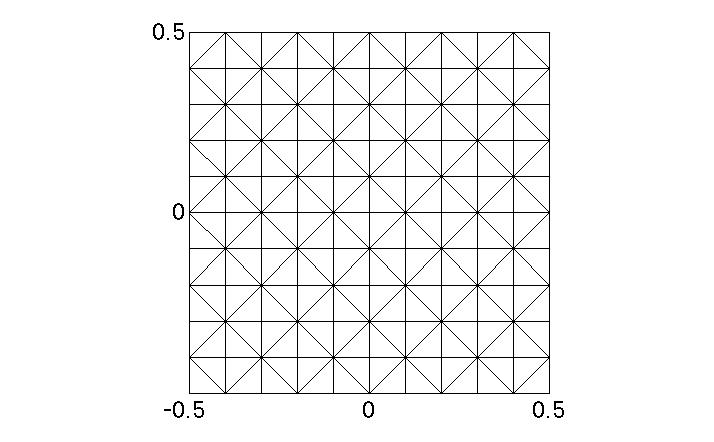
Figure 1: Triangulation $\mathcal{T}_{1/10}$

To simulate random media held inside $D$, $\alpha(\omega,\cdot)$ is generated using a random field $\eta(\omega,\cdot)$ which is a Gaussian random field with an exponential covariance function with correlation length $\ell=0.5$ (cf. [22]), i.e. the following covariance function is used to generate $\eta(\omega,\cdot)$

$$C(\mathbf{x_{1}},\mathbf{x_{2}})=\exp\left(-\frac{\|\mathbf{x_{1}}-\mathbf{x_{2}}\|_{2}}{0.5}\right).$$

For the numerical simulations $\eta(\omega,\cdot)$ is sampled at the center of each element in the mesh. Such two sample realizations of $\eta(\omega,\cdot)$ are given in Figure 2.

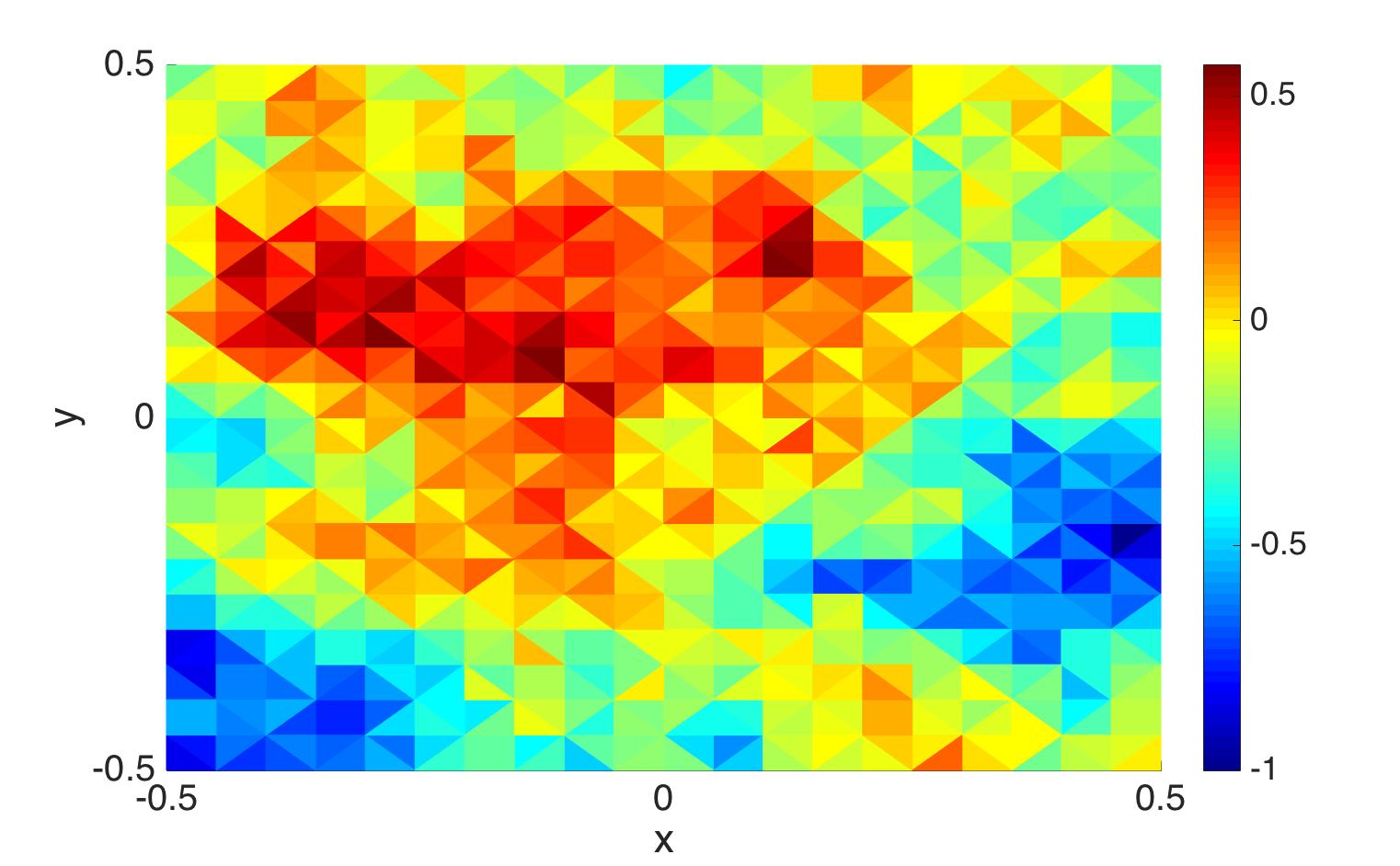
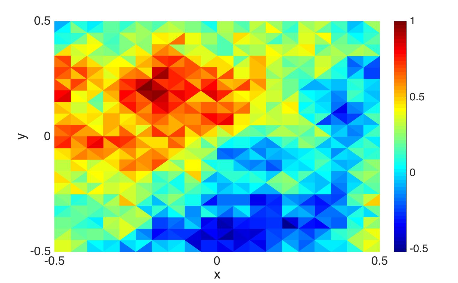
Figure 2: Samples of the random field $\eta(\omega,\cdot)$ generated using an exponential covariance function with covariance length $l=0.5$ on a triangulation parameterized by $h=1/20$.

Due to the difficulty of generating a test problem with a known solution, we use a contrived right-hand side source function of the form

$$\mathbf{f}=\frac{1}{(k\alpha(\omega,\cdot))^{2}r}[e^{{\rm\mathbf{i}}(k\alpha(\omega,\cdot))r}-1,e^{-{\rm\mathbf{i}}(k\alpha(\omega,\cdot))r}-1]^{T},$$

where $r=|\mathbf{x}|$ is the Euclidean length of $\mathbf{x}$. As a baseline, we compare the approximation $\boldsymbol{\Psi}^{h}_{N}$ generated by Algorithm 2 to the classical Monte Carlo approximation $\tilde{\boldsymbol{\Psi}}^{h}$ generated by Algorithm 1.

In our experiments the frequency $k$, the perturbation parameter $\varepsilon$, and the number of modes $N$ are allowed to vary. Other parameters are given the following values:

$$h=1/20,\qquad\mu=1,\qquad\lambda=1,\qquad M=1000,\qquad A=\left[\begin{array}[]{c c}1&0\\ 0&1\end{array}\right].$$

Based on the numerical experiments carried out in [12] we use the following values for our penalty parameters:

$$\gamma_{0,e}=10,\qquad\gamma_{1,e}=0.1,$$

for all edges $e$.

In our first experiment we want to judge the performance of Algorithm 2 when $\varepsilon$ is taken to be small relative to the frequency $k$. For this reason the frequency $k$ is set to be $k=5$ and the perturbation parameter $\varepsilon$ is chosen to be $\varepsilon=1/10$. We expect from Theorem 28 that the relative error between $\boldsymbol{\Psi}^{h}_{N}$ and $\tilde{\boldsymbol{\Psi}}^{h}$ should decrease on the order $\varepsilon^{N}$.

The relative error is plotted versus the $5\varepsilon^{N}$ for $N=1,2,\cdots,7$ in Figure 3. A log scale is used on the vertical access to compare the two. From this plot we note that the relative error is small for all values of $N$, indicating that $\boldsymbol{\Psi}^{h}_{N}$ agrees with $\tilde{\boldsymbol{\Psi}}^{h}$ and thus Algorithm 2 is producing accurate results. We also observe that the relative error decreases at approximately the same order as $\varepsilon^{N}$. What is unexpected in this plot is the fact that the relative error is almost constant between $N=1$ and $N=2$, $N=3$ and $N=4$, and $N=5$ and $N=6$. This behavior is not observed in analogous experiments carried out for the scalar Helmholtz problem in random media (cf. [11]). This behavior might lead one to believe that only odd mode functions contribute to the solution, but we think that this simple explanation may not be correct since two previous mode functions are used to produce a new mode function at every step (cf. (33) and (62)). On the other hand, this is an interesting phenomenon and will be investigated more fully in the near future.

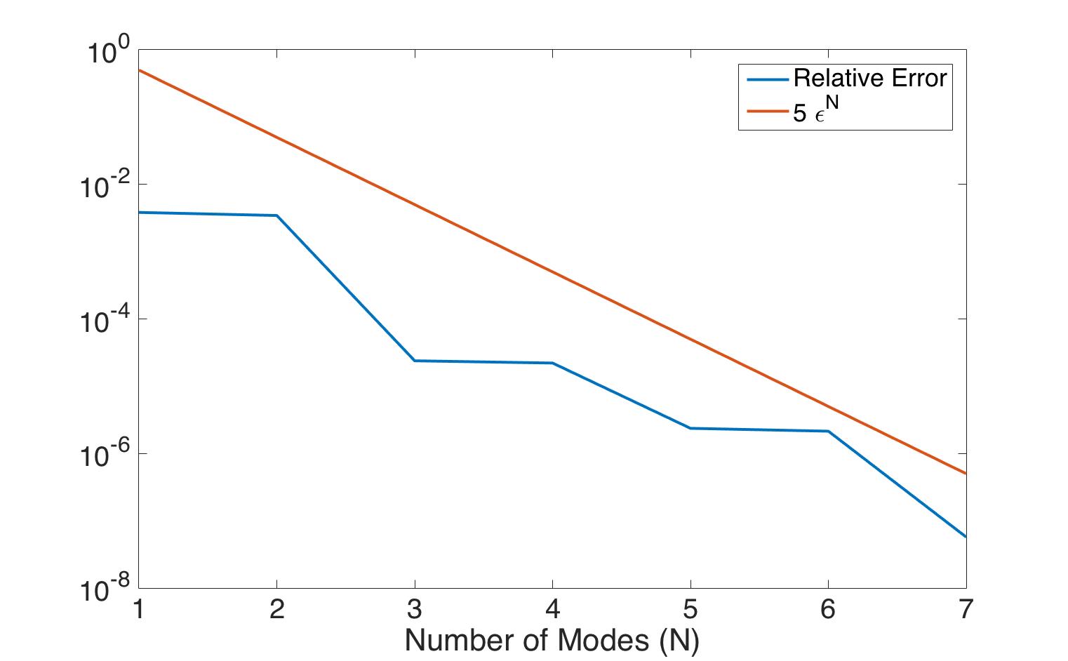
Figure 3: $L^{2}$-norm error between $\Psi^{h}_{N}$ computed using MCIP-DG with the multi-modes expansion and $\tilde{\Psi}^{h}$ computed using the classical MCIP-DG. The vertical access is given in a log scale.

Table 1 summarizes the computation time used to obtain $\boldsymbol{\Psi}^{h}_{N}$ using Algorithm 2 with various values of $N$ and the computation time used to obtain $\tilde{\boldsymbol{\Psi}}^{h}$ using Algorithm 1. All experiments are performed on the same iMac computer with a 2 GHz Intel Core i7 processor. From Table 1 we observe that Algorithm 2 produces accurate approximations with far less computation time than Algorithm 1. In fact, Algorithm 2 improves performance by at least one order of magnitude. We also observe that the computation time used for Algorithm 2 increases linearly as the number of modes $N$ is increased. This is to be expected.

Approximation	CPU Time (s)
$\tilde{\Psi}^{h}$	$21680$
$\Psi^{h}_{1}$	$149$
$\Psi^{h}_{2}$	$335$
$\Psi^{h}_{3}$	$522$
$\Psi^{h}_{4}$	$709$
$\Psi^{h}_{5}$	$897$
$\Psi^{h}_{6}$	$1085$
$\Psi^{h}_{7}$	$1272$

Table 1: CPU times required to compute the MCIP-DG multi-modes approximation $\Psi^{h}_{N}$ and classical MCIP-DG approximation $\tilde{\Psi}^{h}$.

For our second set of numerical experiments our goal is to check the accuracy of Algorithm 2 when the size of the perturbation parameter $\varepsilon$ is allowed to grow larger. In this set of experiments the frequency $k$ is set to be $10$ and the perturbation parameter is tested at $\varepsilon=0.05,0.1,0.5,0.8$.

Table 2 shows the relative error associated $\boldsymbol{\Psi}^{h}_{3}$ produced by Algorithm 2 using $N=3$ modes. In this table we observe that the approximations associated with $\varepsilon=0.05$ and $0.1$ are accurate as demonstrated by their small relative errors. For $\varepsilon=0.5$ and $0.8$ Theorem 28 implies a larger number of modes $N$ might be needed to produce more accurate approximations. With this point in mind, Table 3 records the relative error associated with these values of $\varepsilon$ along with a larger number of modes $N$. From this table we observe that for $\varepsilon=0.5$ the relative error does not strictly decrease, but when $N=7$ it does produce a more accurate approximation. For $\varepsilon=0.8$ using a larger $N$ does not seem to help decrease the relative error. This is to be expected since our convergence theory requires $\varepsilon$ to be small relative to the size of $k$ and thus for $\varepsilon$ large, Algorithm 2 will no longer produce accurate solutions.

Lastly, Figures 4–7 show the solutions $\boldsymbol{\Psi}^{h}_{7}$ produced by Algorithm 2 and sample realizations $\mathbf{U}^{h}_{7}$ for $k=10$, $h=1/20$, and $\varepsilon=0.05$.

$\varepsilon$	$0.05$	$0.1$	$0.5$	$0.8$
Relative $L^{2}$ Error	$1.4559\times 10^{-5}$	$9.7719\times 10^{-5}$	$0.0399$	$0.2216$

Table 2: $L^{2}$-norm relative error between the multimodes expansion approximation $\Psi^{h}_{3}$ and the classical Monte Carlo approximation $\tilde{\Psi}^{h}$.

$\varepsilon$	$N=4$	$N=5$	$N=6$	$N=7$
$0.5$	$0.1037$	$0.0154$	$0.0450$	$0.0069$
$0.8$	$0.5218$	$0.2172$	$0.5644$	$0.2155$

Table 3: $L^{2}$-norm relative error between the multimodes expansion approximation $\Psi^{h}_{N}$ and the classical Monte Carlo approximation $\tilde{\Psi}^{h}$.

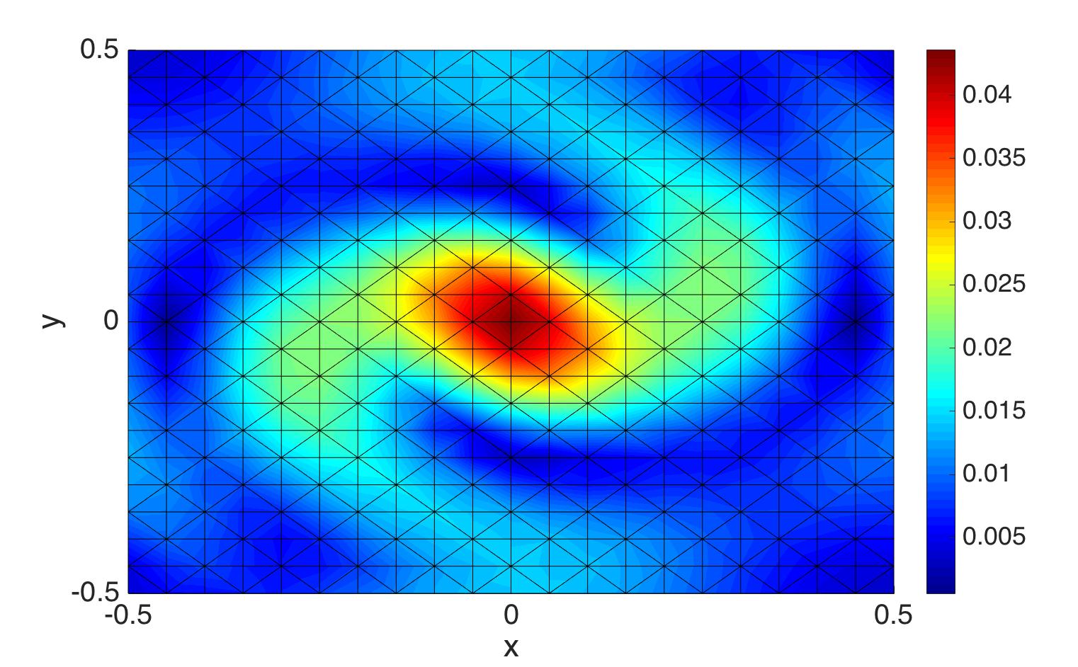
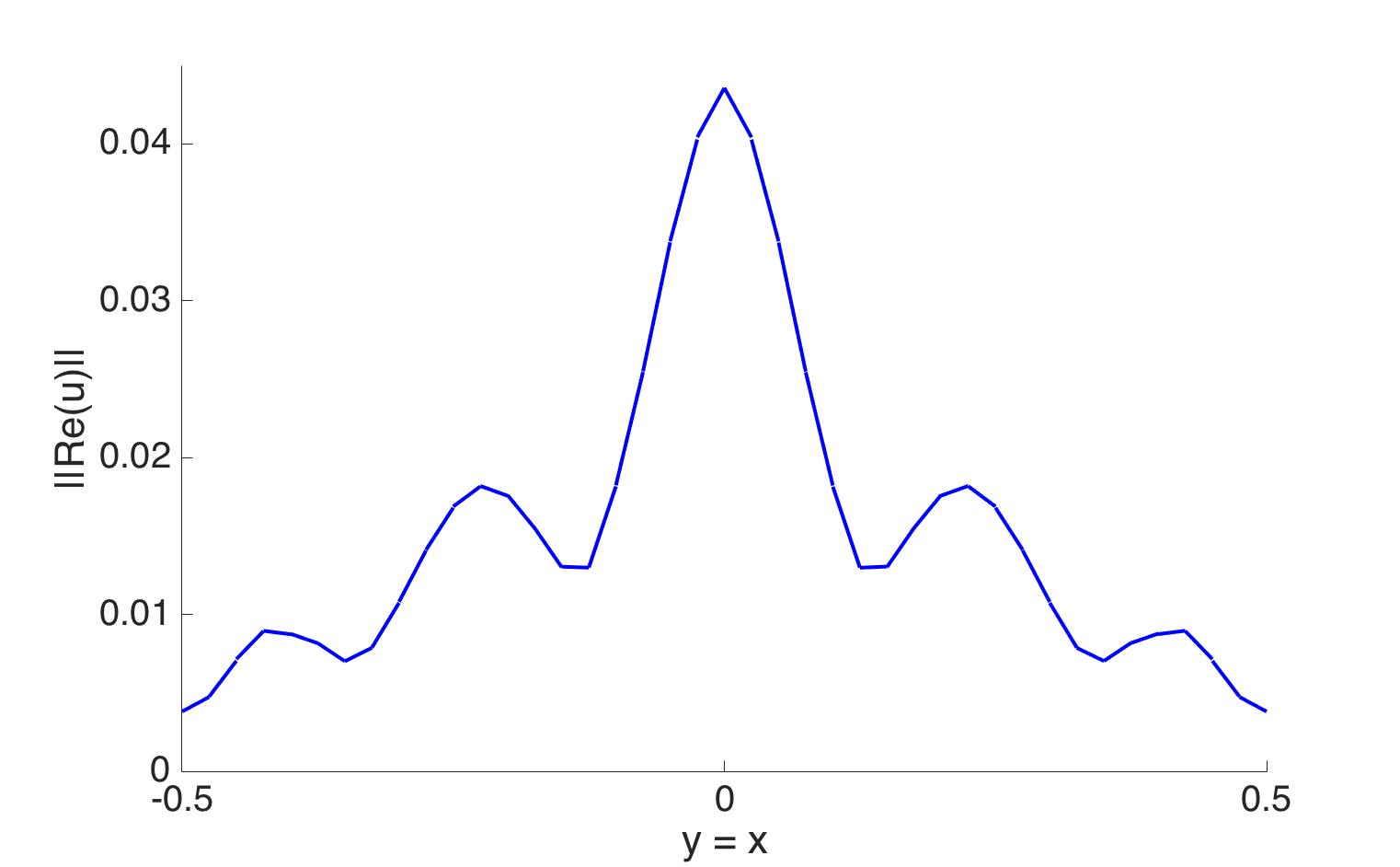
Figure 4: Plot of the statistical average ${\rm Re}\big{(}\Psi^{h}_{7}\big{)}$ on the domain $[-0.5,0.5]\times[-0.5,0.5]$ (left) and on the cross section $y=x$ (right) for $k=10$, $h=1/20$, $\varepsilon=0.05$, and $M=1000$.

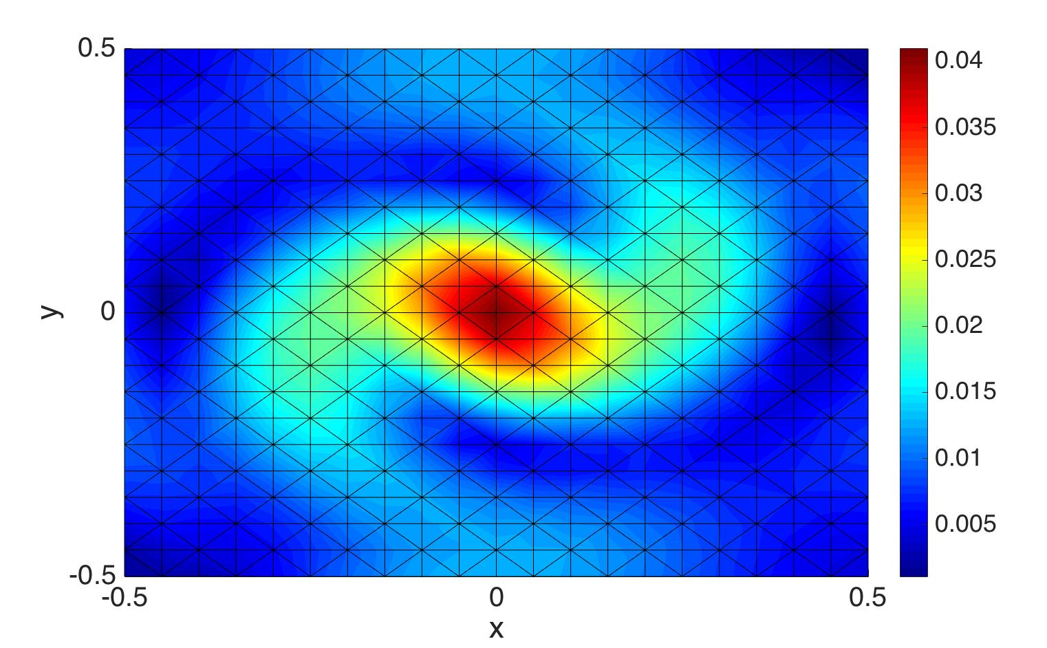
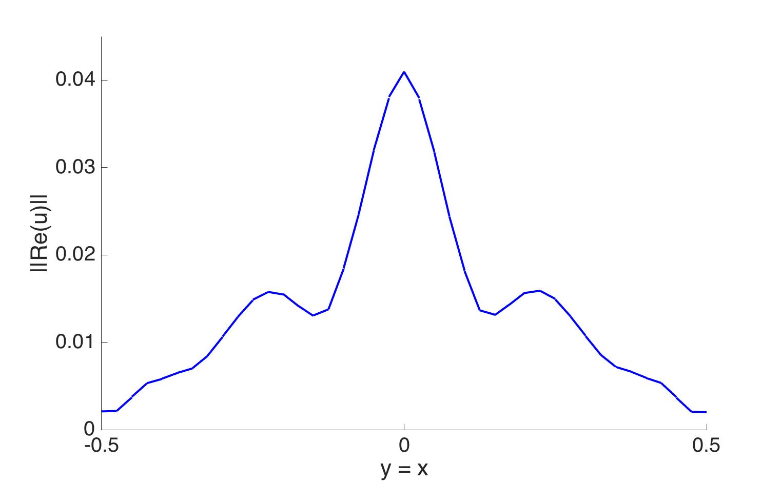
Figure 5: Plot of the sample realization ${\rm Re}\big{(}\mathbf{U}^{h}_{7}\big{)}$ on the domain $[-0.5,0.5]\times[-0.5,0.5]$ (left) and on the cross section $y=x$ (right) for $k=10$, $h=1/20$, $\varepsilon=0.05$, and $M=1000$.

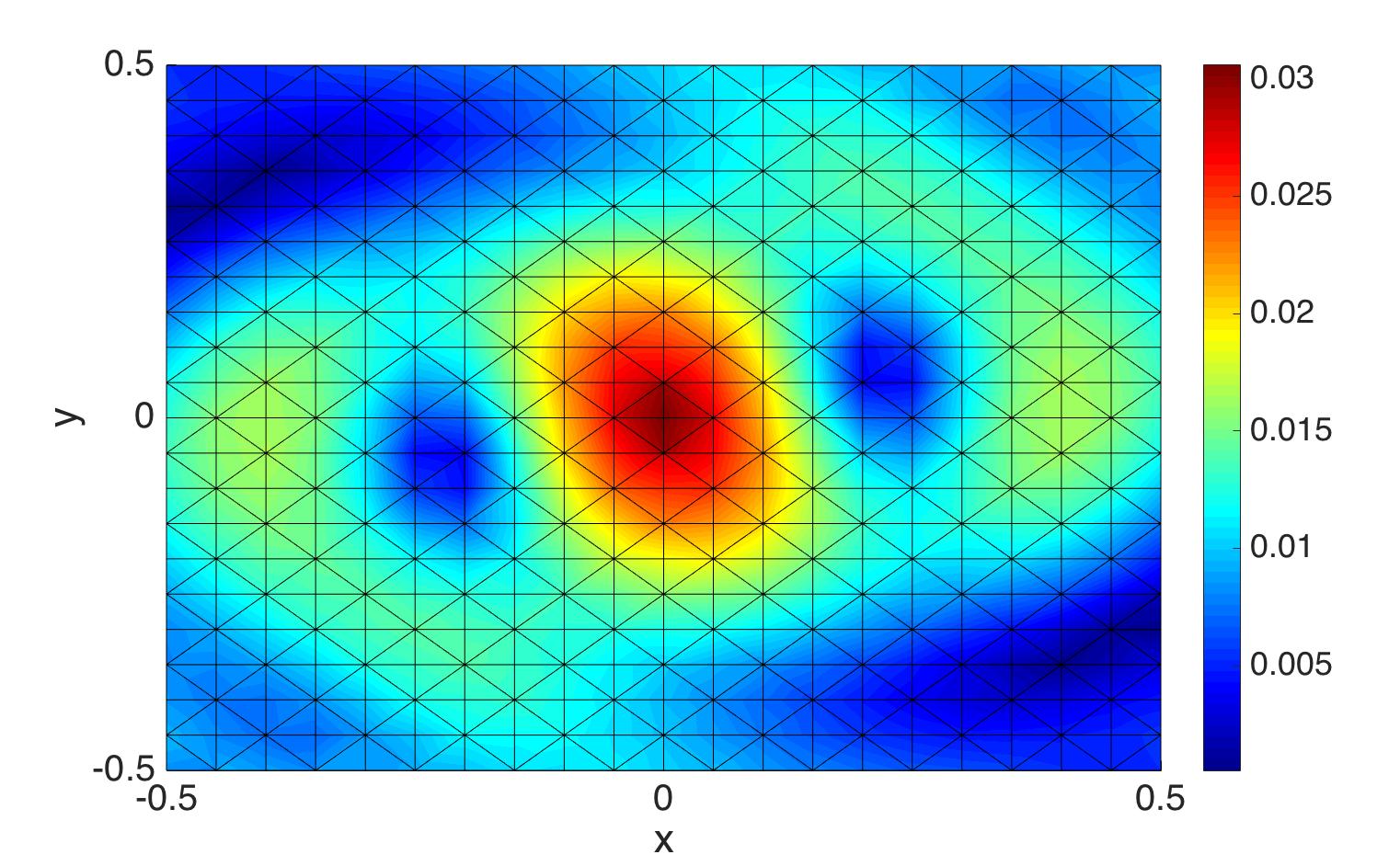
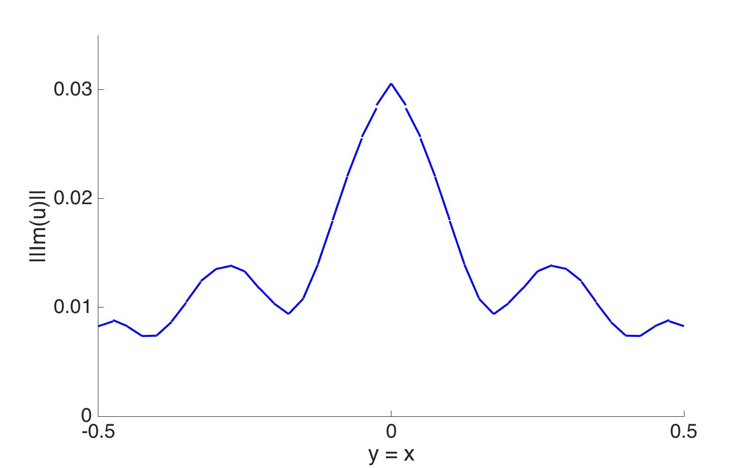
Figure 6: Plot of the statistical average ${\rm Im}\big{(}\Psi^{h}_{7}\big{)}$ on the domain $[-0.5,0.5]\times[-0.5,0.5]$ (left) and on the cross section $y=x$ (right) for $k=10$, $h=1/20$, $\varepsilon=0.05$, and $M=1000$.

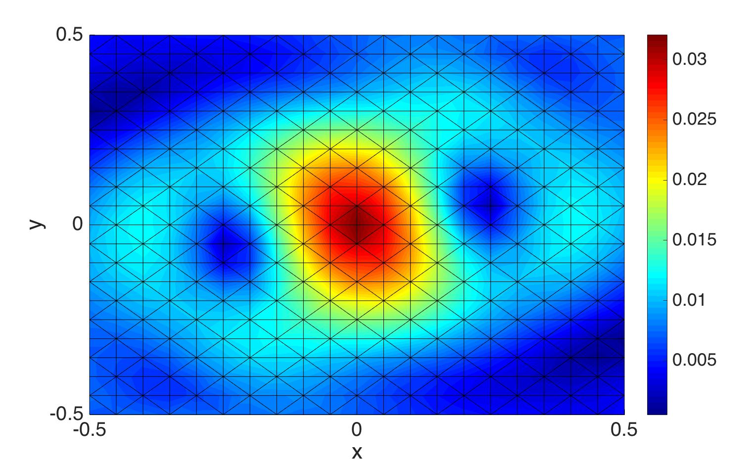
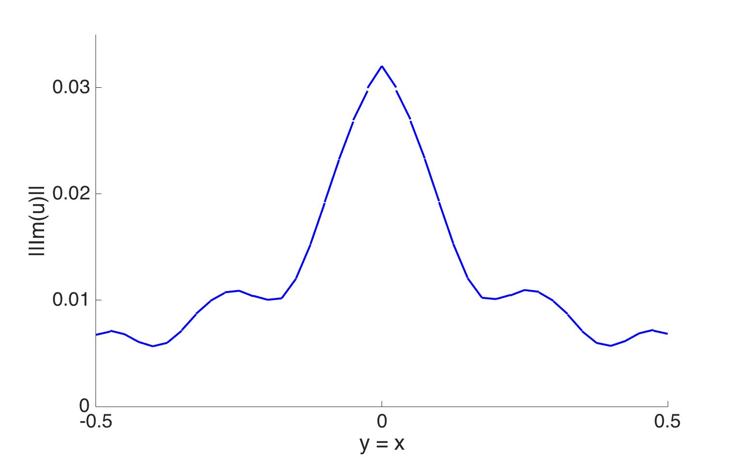
Figure 7: Plot of the sample realization ${\rm Im}\big{(}\mathbf{U}^{h}_{7}\big{)}$ on the domain $[-0.5,0.5]\times[-0.5,0.5]$ (left) and on the cross section $y=x$ (right) for $k=10$, $h=1/20$, $\varepsilon=0.05$, and $M=1000$.

6 Extension to more general random media

The multi-modes Monte Carlo IP-DG method we developed above is applicable only to weakly random media in the sense that the coefficient $\alpha$ in the SPDE system must have the form $\alpha(\omega,x)=\alpha_{0}(x)+\varepsilon\eta(\omega,x)$ and $\varepsilon$ is not large. For more general random media, its density $\rho$ or the coefficient $\alpha=\sqrt{\rho}$ may not have the required “weak form”. A natural question is whether and how the above multi-modes Monte Carlo IP-DG method can be extended to cover more general and non-weak random media. A short answer to this question is positive. To this end, our main idea for overcoming this difficulty is first to rewrite $\alpha(x,\omega)$ as the required form $\alpha_{0}(x)+\varepsilon\eta(\omega,x)$, then to apply the above weakly random media framework. There are at least two approaches to do such a re-writing, the first one is to utilize the well-known Karhunen-Loève expansion and the second is to use a recently developed stochastic homogenization theory [7]. Since the second approach is more involved and lengthy to describe, below we only outline the first approach.

For many geoscience and material science applications, the random media can be described by a Gaussian random field [16, 19, 22]. Let $\overline{\alpha}(x)$ and $C(x,y)$ denote the mean and covariance function of the Gaussian random field $\alpha(\omega,x)$, respectively. Two of the most widely used covariance functions in geoscience and materials science are $C(x,y)=\exp(|x-y|^{m}/\ell)$ for $m=1,2$ and $0<\ell<1$ (cf. [22, Chapter 7]. Here $\ell$ is often called correlation length which determines the range of the noise. The well-known Karhunen-Loève expansion for $\alpha(\omega,x)$ takes the following form (cf. [22]):

$$\alpha(\omega,x)=\overline{\alpha}(x)+\sum_{k=1}^{\infty}\sqrt{\lambda_{k}}\phi_{k}(x)\xi_{k}(\omega),$$

where $\{(\lambda_{k},\phi_{k})\}_{k\geq 1}$ is the eigenset of the (self-adjoint) covariance operator and $\{\xi_{k}\sim N(0,1)\}_{k\geq 1}$ are i.i.d. random variables. It can be shown that in many cases there holds $\lambda_{k}=O(\ell^{r})$ for some $r>1$ depending on the spatial domain $D$ where the PDE is defined (cf. [22, Chapter 7]), that is the case when $D$ is rectangular. Consequently, we can write

$$\alpha(\omega,x)=\overline{\alpha}(x)+\sqrt{\lambda_{1}}\zeta(x,\omega),\qquad\zeta(x,\omega):=\sum_{k=1}^{\infty}\sqrt{\frac{\lambda_{k}}{\lambda_{1}}}\,\phi_{k}(x)\xi_{k}(\omega),$$

Thus, setting $\varepsilon=O(\ell^{\frac{r}{2}})$ gives rise to $\alpha(\omega,x)=\overline{\alpha}+\varepsilon\zeta$, which is the required “weak form” consisting of a deterministic background field plus a small random perturbation. So we just showed that in many cases a given random field $\alpha$ can be rewritten into the required “weak form”. Therefore, our multi-modes Monte Carlo IP-DG method can still be applied to such general random media.

It should be pointed out that the classical Karhunen-Loève expansion may be replaced by other types of expansion formulas which may result in more efficient multi-modes Monte Carlo methods. Finally, we also remark that the IP-DG method can be replaced by any other space discretization method such as finite difference, finite element, and spectral method in Algorithm 2.

References

[1]
I. Babuška, F. Nobile, and R. Tempone.
A stochastic collocation method for elliptic partial differential
equations with random input data.
SIAM Rev., 52:317 – 355, 2010.
[2]
I. Babuška, R. Tempone, and G.E. Zouraris.
Galerkin finite element approximations of stochastic elliptic
partial differential equations.
SIAM J. Numer. Anal., 42:800 – 825, 2004.
[3]
I. Babuška, R. Tempone, and G.E. Zouraris.
Solving elliptic boundary value problems with uncertain coefficients
by the finite element method: the stochastic formulation.
Comput. Methods Appl. Mech. Engrg, 194:1251 – 1294, 2005.
[4]
R. Caflisch.
Monte Carlo and quasi-Monte Carlo methods.
Acta Numerica, 7:1–49, 1998.
[5]
P. Cummings and X. Feng.
Sharp regularity coefficient estimates for complex-valued acoustic
and elastic Helmholtz equations.
Mathematical Models and Methods in Applied Sciences, 16:139 –
160, 2006.
[6]
M. Deb, I. Babuška, and J. Oden.
Solution of stochastic partial differential equations using
Galerkin finite element techniques.
Comput. Methods Appl. Mech. Engrg., 190:6359 – 6372, 2001.
[7]
M. Duerinckx, A. Gloria, and F. Otto.
The structure of fluctuations in stochastic homogenization.
arXiv:1602.01717[math.AP].
[8]
M. Eiermann, O. Ernst, and E. Ullmann.
Computational aspects of the stochastic finite element method.
Proceedings of ALGORITMY, pages 1–10, 2005.
[9]
B. Engquist and A. Majda.
Radiation bounday conditions for acoustic and elastics wave
calculations.
Comm. Pure Appl. Math., 32(3):314 – 358, 1979.
[10]
O. Ernst and M. Gander.
Why it is difficult to solve Helmholtz problems with classical
iterative methods?
In I. Graham, T. Hou, O. Lakkis, and R. Scheichl, editors, Numerical Analysis of Multiscale Problems, Lecture Notes in Computational
Science and Engineering 83, pages 325 – 363. Springer Verlag, 2012.
[11]
X. Feng, J. Lin, and C. Lorton.
An efficient numerical method for acoustic wave scattering in random
media.
SIAM/ASA J. UQ, 3:790 – 822, 2015.
[12]
X. Feng and C. Lorton.
An unconditionally stable discontinuous Galerkin method for the
elastic Helmholtz equations with large frequency.
to appear in J. Scient. Comput.
[13]
X. Feng and H. Wu.
Discontinuous Galerkin methods for the Helmholtz equation with
large wave numbers.
SIAM J. Numer. Anal., 47:2872 – 2896, 2009.
[14]
X. Feng and H. Wu.
hp-discontinuous Galerkin methods for the Helmholtz equation with
large wave numbers.
Math. Comp., 80:1997 – 2024, 2011.
[15]
X. Feng and H. Wu.
An absolutely stable discontinuous Galerkin method for the
indefinite time-harmonic Maxwell equations with large wave number.
SIAM J. Numer. Anal., 52:2356 – 2380, 2014.
[16]
J. Fouque, J. Garnier, G. Papanicolaou, and K. Solna.
Wave Propogation and Time Reversal in Randomly Layered Media,
volume 56 of Stochastic Modeling and Applied Probability.
Springer, 2007.
[17]
D. Gilbarg and N.S. Trudinger.
Elliptic Partial Differential Equations of Second Order.
Classics in Mathematics. Springer Verlag, Berlin, 2001.
reprint of the 1998 edition.
[18]
P. Grisvard.
Singularities in boundary value problems, volume 22 of Recherches en Mathématiques Appliquées [Research in Applied
Mathematics].
Masson, Paris; Springer-Verlag, Berlin, 1992.
[19]
A. Ishimaru.
Wave Propagation and Scattering in Random Media.
IEEE Press, New York, 1997.
[20]
O. A. Ladyženskaja, V. A. Solonnikov, and N. N. Ural′ceva.
Linear and quasilinear equations of parabolic type.
Translated from the Russian by S. Smith. Translations of Mathematical
Monographs, Vol. 23. American Mathematical Society, Providence, R.I., 1968.
[21]
K. Liu and B. Rivière.
Discontinuous Galerkin methods for elliptic partial differential
equations with random coefficients.
Int. J. Computer Math., 90(11):2477 – 2490, 2013.
[22]
G. Lord, C. Powell, and T. Shardlow.
An Introduction to Computational Stochastic PDEs.
Cambridge University Press, 2014.
[23]
C. Lorton.
Numerical methods and algorithms for high frequency wave
scattering problems in homogeneous and random media.
PhD thesis, The University of Tennessee, August 2014.
[24]
A. J. Nitsche.
On Korn’s second inequality.
R.A.I.R.O. Anal. Numér., 15:237–248, 1998.
[25]
L. Roman and M. Sarkis.
Stochastic Galerkin method for elliptic SPDEs: A white noise
approach.
Discret. Contin. Dyn. S., 6:941 – 955, 2006.
[26]
D. Xiu and G. Karniadakis.
Modeling uncertainty in steady state diffusion problems via
generalized polynomial chaos.
Comput. Methods Appl. Mech. Engrg., 191:4927 – 4948, 2002.
[27]
D. Xiu and G. Karniadakis.
The Wiener-Askey polynomial chaos for stochastic differential
equations.
SIAM J. Sci. Comput., 24:619 – 644, 2002.