Equilibration and aging of liquids of non-spherically interacting particles

Abstract

The non-equilibrium self-consistent generalized Langevin equation theory of irreversible processes in liquids is extended to describe the positional and orientational thermal fluctuations of the instantaneous local concentration profile $n(\mathbf{r},\bm{\Omega},t)$ of a suddenly-quenched colloidal liquid of particles interacting through non spherically-symmetric pairwise interactions, whose mean value $\overline{n}(\mathbf{r},\bm{\Omega},t)$ is constrained to remain uniform and isotropic, $\overline{n}(\mathbf{r},\bm{\Omega},t)=\overline{n}(t)$. Such self-consistent theory is cast in terms of the time-evolution equation of the covariance $\sigma(t)=\overline{\delta n_{lm}(\mathbf{k};t)\delta n^{\dagger}_{lm}(\mathbf{k};t)}$ of the fluctuations $\delta n_{lm}(\mathbf{k};t)=n_{lm}(\mathbf{k};t)-\overline{n_{lm}}(\mathbf{k};t)$ of the spherical harmonics projections $n_{lm}(\mathbf{k};t)$ of the Fourier transform of $n(\mathbf{r},\bm{\Omega},t)$. The resulting theory describes the non-equilibrium evolution after a sudden temperature quench of both, the static structure factor projections $S_{lm}(k,t)$ and the two-time correlation function $F_{lm}(k,\tau;t)\equiv\overline{\delta n_{lm}(\mathbf{k},t)\delta n_{lm}(\mathbf{k},t+\tau)}$, where $\tau$ is the correlation delay time and $t$ is the evolution or waiting time after the quench. As a concrete and illustrative application we use the resulting self-consistent equations to describe the irreversible processes of equilibration or aging of the orientational degrees of freedom of a system of strongly interacting classical dipoles with quenched positional disorder.

I Introduction

The fundamental description of dynamically arrested states of matter is a crucial step towards understanding the properties of very common amorphous solid materials such as glasses and gels angellreview1 ; ngaireview1 ; sciortinotartaglia , and of more technologically specialized materials, such as spin glasses spinglassbook ; gingras ; biltmo . The main fundamental challenge posed by these materials derives from their inability to reach thermodynamic equilibrium within experimental times, and from the fact that their properties depend on the protocol of preparation, in obvious contrast with materials that have genuinely attained thermodynamic equilibrium. Understanding the origin of this behaviour falls outside the realm of classical and statistical thermodynamics, and must unavoidably be addressed from the perspective of a non-equilibrium theory degrootmazur ; keizer ; casasvazquez0 . In fact, a major challenge for statistical physics is to develop a microscopic theory able to predict the properties of glasses and gels in terms not only of the intermolecular forces and applied external fields, but also in terms of the protocol of preparation of the material.

First-principles theoretical frameworks exist, leading to quantitative predictions of the dynamic properties of structural glass forming liquids near their dynamical arrest transitions, one of the best-known being mode coupling theory (MCT) goetze1 ; goetze2 . However, this theory, as well as the equilibrium version of the self-consistent generalized Langevin equation (SCGLE) theory of dynamical arrest todos1 ; todos2 , are meant to describe the dynamics of fully equilibrated liquids. Hence, the phenomenology of the transient time-dependent processes, such as aging, occurring during the amorphous solidification of structural glass formers, falls completely out of the scope of these equilibrium theories. Thus, it is important to attempt their extension to describe these non-stationary non-equilibrium structural relaxation processes, which in the end constitute the most fundamental kinetic fingerprint of glassy behavior.

In an attempt to face this challenge, in 2000 Latz latz proposed a formal non-equilibrium extension of MCT which, however, has not yet found a specific quantitative application. In the meanwhile, the SCGLE theory has recently been extended to describe non-stationary non-equilibrium processes in glass-forming liquids nescgle1 ; nescgle2 . The resulting non-equilibrium theory, referred to as the non-equilibrium self-consistent generalized Langevin equation (NE-SCGLE) theory, was derived within the fundamental framework provided by a non-stationary extension nescgle1 of Onsager’s theory of linear irreversible thermodynamics onsager1 ; onsager2 and of time-dependent thermal fluctuations onsagermachlup1 ; onsagermachlup2 , with an adequate extension delrio ; faraday to allow for the description of memory effects.

The NE-SCGLE theory thus derived, aimed at describing non-equilibrium relaxation phenomena in general nescgle1 , leads in particular nescgle2 to a simple and intuitive but generic description of the essential behavior of the non-stationary and non-equilibrium structural relaxation of glass-forming liquids near and beyond its dynamical arrest transition. This was explained in detail in Ref. nescgle3 in the context of a model liquid of soft-sphere particles. The recent comparison nescgle7 of the predicted scenario with systematic simulation experiments of the equilibration and aging of dense hard-sphere liquids, indicates that the accuracy of these predictions go far beyond the purely qualitative level, thus demonstrating that the NE-SCGLE theory is a successful pioneering first-principles statistical mechanical approach to the description of these fully non-equilibrium phenomena.

As an additional confirmation, let us mention that for model liquids with hard-sphere plus attractive interactions, the NE-SCGLE theory predicts a still richer and more complex scenario, involving the formation of gels and porous glasses by arrested spinodal decomposition nescgle5 ; nescgle6 . As we know, quenching a liquid from supercritical temperatures to a state point inside its gas-liquid spinodal region, normally leads to the full phase separation through a process that starts with the amplification of spatial density fluctuations of certain specific wave-lengths cahnhilliard ; cook ; furukawa . Under some conditions, however, this process may be interrupted when the denser phase solidifies as an amorphous sponge-like non-equilibrium bicontinuous structure luetalnature ; sanz ; gibaud ; foffi ; helgeson , typical of physical gels zaccarellireviewgels . This process is referred to as arrested spinodal decomposition, and has been observed in many colloidal systems, including colloid-polymer mixtures luetalnature , mixtures of equally-sized oppositely-charged colloids sanz , lysozyme protein solutions gibaud , mono- and bi-component suspensions of colloids with DNA-mediated attractions foffi , and thermosensitive nanoemulsions helgeson . From the theoretical side, it was not clear how to extend the classical theory of spinodal decomposition cahnhilliard ; cook ; furukawa to include the possibility of dynamic arrest, or how to incorporate the characteristic non-stationarity of spinodal decomposition, in existing theories of glassy behavior berthierreview . In Refs. nescgle5 and nescgle6 it has been shown that the NE-SCGLE theory provides precisely this missing unifying theoretical framework.

Recently the NE-SCGLE theory was extended to multi-component systems nescgle4 , thus opening the route to the description of more complex non-equilibrium amorphous states of matter. Until now, however, the NE-SCGLE theory faces the limitation of referring only to liquids of particles with radially symmetric pairwise interparticle forces, thus excluding its direct comparison with the results of important real and simulated experiments involving intrinsically non-spherical particles arrozchino ; weeks and, in general, particles with non-radially symmetric interactions. The present work constitutes a first step in the direction of extending the NE-SCGLE theory to describe the irreversible evolution of the static and dynamic properties of a Brownian liquid constituted by particles with non-radially symmetric interactions, in which the orientational degrees of freedom are essential.

More concretely, the main purpose of the present paper is to describe the theoretical derivation of the NE-SCGLE time-evolution equations for the spherical harmonics projections $S_{lm,lm}(k;t)$, $F_{lm,lm}(k,\tau;t)$, and $F_{lm,lm}^{S}(k,\tau;t)$, of the non-equilibrium and non-stationary static structure factor $S(\mathbf{k},\bm{\Omega};t)$ and of the collective and self intermediate scattering functions $F(\mathbf{k},\bm{\Omega},\bm{\Omega}^{\prime},\tau;t)$ and $F^{S}(\mathbf{k},\bm{\Omega},\bm{\Omega^{\prime}},\tau;t)$. For this, we start from the same general and fundamental framework provided by the non-stationary extension of Onsager’s theory, developed in Ref. nescgle1 to discuss the spherical case. The result of the present application are Eqs. (39)-(45) below, in which $\tau$ is the delay time, and $t$ is the evolution (or “waiting”) time after the occurrence of the instantaneous temperature quench. The solution of these equations describe the non-equilibrium (translational and rotational) diffusive processes occurring in a colloidal dispersion after an instantaneous temperature quench, with the most interesting prediction being the aging processes that occur when full equilibration is prevented by conditions of dynamic arrest.

Although this paper only focuses on the theoretical derivation of the NE-SCGLE equations, as an illustration of the possible concrete applications of the extended non-equilibrium theory, here we also solve the resulting equations for one particular system and condition. We refer to a liquid of dipolar hard-spheres (DHS) with fixed positions and subjected to a sudden temperature quench. This is a simple model of the irreversible evolution of the collective orientational degrees of freedom of a system of strongly interacting magnetic dipoles with fixed but random positions. Although this particular application by itself has its own intrinsic relevance in the context of disordered magnetic materials, the main reason to choose it as the illustrative example is that Eqs. (39)-(45) describe coupled translational and rotational dynamics, whose particular case $l=0$ coincide with the radially-symmetric case, already discussed in detail in Refs. nescgle3 ; nescgle4 ; nescgle5 . Thus, the most novel features are to be expected in the non-equilibrium rotational dynamics illustrated in this exercise.

Just like in the case of liquids formed by spherical particles, the development of the NE-SCGLE theory for liquids of non-spherical particles requires the previous development of the equilibrium version of the corresponding SCGLE theory. Such an equilibrium SCGLE theory for non-spherical particles, however, was previously developed by Elizondo-Aguilera et al. gory1 , following to a large extent the work of Schilling and collaborators schilling1 ; schilling2 ; schilling3 on the extension of mode coupling theory for this class of systems. Thus, we start our discussions in section II with a brief review of the main elements of the non spherical equlibrium SCGLE theory and its application to dynamical arrest in systems formed by colloidal interacting particles with non spherical potentials.

In section III we outline the conceptual basis and the main steps involved in the derivation of the non-equilibrium extension of the SCGLE theory for glass-forming liquids of non-spherical particles. In the same section we summarize the resulting set of self consistent equations which constitutes this extended theory. In section IV, we introduce a simplified model for interacting dipoles randomly distributed in space and apply our equations to investigate the slow orientational dynamics as well as the aging and equilibration processes of the system near its “spin glass”-like transitions. Finally in section V we summarize our main conclusions.

II Equilibrium SCGLE theory of Brownian liquids of non-spherical particles.

In this section we briefly describe the equilibrium SCGLE theory of the dynamics of liquids formed by non-spherical particles developed by Elizondo-Aguilera et al. gory1 . We first describe the main properties involved in this description and then summarize their time-evolution equations, which constitute the essence of the SCGLE theory.

II.1 Collective description of the translational and orientational degrees of freedom.

Let us start by considering a liquid formed by $N$ identical non-spherical colloidal particles in a volume $V$ gory1 , each having mass $m$ and inertia tensor $\mathbf{I}$. The translational degrees of freedom are described by the vectors $\mathbf{r}^{N}\equiv(\mathbf{r}_{1},...,\mathbf{r}_{N})$ and $\mathbf{p}^{N}\equiv(\mathbf{p}_{1},...,\mathbf{p}_{N})$, where $\mathbf{r}_{n}$ denotes the center-of-mass position vector of the $n$th-particle and $\mathbf{p}_{n}\equiv md\mathbf{r}_{n}/dt=m\mathbf{v}_{n}(t)$ is the associated linear momentum. Similarly, the orientational degrees of freedom are described by the abstract vectors $\mathbf{\Omega}^{N}\equiv(\mathbf{\Omega}_{1},...,\mathbf{\Omega}_{N})$ and $\mathbf{L}^{N}\equiv(\mathbf{L}_{1},...,\mathbf{L}_{N})$, where $\mathbf{\Omega}_{n}$ denotes the Euler angles which specify the orientation of the $n$th molecule, and $\mathbf{L}_{n}=\mathbf{I}(\mathbf{\Omega}_{n})\bm{\omega}_{n}$ is the corresponding angular momentum, so that $\bm{\omega}_{n}$ denotes the angular velocity. Let us now assume that the potential energy $U(\mathbf{r}^{N},\bm{\Omega}^{N})$ of the interparticle interactions is pairwise additivity, i.e., that

$$U(\mathbf{r}^{N},\bm{\Omega}^{N})=\sum_{n,n^{\prime}=1}^{N}u(\mathbf{r}_{n},\mathbf{r}_{n^{\prime}};\bm{\Omega}_{n},\bm{\Omega}_{n^{\prime}}),$$ (1)

where $u(\mathbf{r}_{n},\mathbf{r}_{n^{\prime}};\bm{\Omega}_{n},\bm{\Omega}_{n^{\prime}})$ is the interaction potential between particles $n$ and $n^{\prime}$. In the particular case of axially-symmetric particles, that we shall have in mind here, the third Euler angle is actually redundant, and hence, $\bm{\Omega}_{n}=\bm{\Omega}_{n}(\theta_{n},\phi_{n})$.

The most basic observable in terms of which we want to describe the dynamical properties of a non-spherical colloidal system is the time dependent microscopic one-particle density

$$n(\mathbf{r},\bm{\Omega};t)\equiv(1/\sqrt{N})\sum_{n=1}^{N}\delta(\mathbf{r}-\mathbf{r}_{n}(t))\delta(\bm{\Omega}-\bm{\Omega}_{n}(t)).$$ (2)

Given that $\bm{\Omega}=\bm{\Omega}(\theta,\phi)$, any function $f(\mathbf{r},\bm{\Omega})$ can be expanded with respect to plane waves and spherical harmonics as

$$f(\mathbf{r},\bm{\Omega})=\frac{1}{V}\frac{1}{\sqrt{4\pi}}\int d\mathbf{k}\sum_{lm}(i)^{l}f_{lm}(\mathbf{k})e^{-i\mathbf{k}\cdot\mathbf{r}}Y^{*}_{lm}(\bm{\Omega})$$ (3)

where

$$f_{lm}(\mathbf{k})=\sqrt{4\pi}i^{l}\int_{V}d\mathbf{r}\int d\bm{\Omega}f(\mathbf{r},\bm{\Omega})e^{-i\mathbf{k}\cdot\mathbf{r}}Y_{lm}(\bm{\Omega}).$$ (4)

Thus, using Eq. (2) in (3) and (4), we may define the so-called tensorial density modes

$$n_{lm}(\mathbf{k},t)=\sqrt{\frac{4\pi}{N}}i^{l}\sum_{n=1}^{N}e^{i\mathbf{k}\cdot\mathbf{r}_{n}(t)}Y_{lm}(\bm{\Omega}_{n}(t)),$$ (5)

and hence, we can define the following two-time correlation functions,

$$F_{lm;l^{\prime}m^{\prime}}(\mathbf{k},\tau;t) \equiv \langle\delta n^{*}_{lm}(\mathbf{k},t+\tau)\delta n_{l^{\prime}m^{\prime}}(\mathbf{k},t)\rangle$$

$$= \frac{4\pi}{N}i^{l-l^{\prime}}\sum_{n\neq n^{\prime}}^{N}\Big{\langle}e^{i\mathbf{k}\cdot[\mathbf{r}_{n}(t+\tau)-\mathbf{r}_{n^{\prime}}(t)]}Y_{lm}^{*}(\bm{\Omega}_{n}(t+\tau))Y_{l^{\prime}m^{\prime}}(\bm{\Omega}_{n^{\prime}}(t))\Big{\rangle},$$

where $\delta n_{lm}(\mathbf{k},t)\equiv n_{lm}(\mathbf{k},t)-\langle n_{lm}(\mathbf{k},t)\rangle$.

We also define for completeness the self components

$$n^{S}_{lm}(\mathbf{k},t)\equiv\sqrt{4\pi}i^{l}e^{i\mathbf{k}\cdot\mathbf{r}_{T}(t)}Y_{lm}(\bm{\Omega}_{T}(t)),$$ (7)

and the corresponding two-time correlation functions

$$F^{S}_{lm;l^{\prime}m^{\prime}}(\mathbf{k},\tau;t)\equiv\langle n^{S*}_{lm}(\mathbf{k},t+\tau)n^{S}_{l^{\prime}m^{\prime}}(\mathbf{k},t)\rangle$$

$$=4\pi i^{l-l^{\prime}}\Big{\langle}e^{i\mathbf{k}\cdot[\mathbf{r}_{T}(t+\tau)-\mathbf{r}_{T}(t)]}Y_{lm}(\bm{\Omega}_{T}(t+\tau))Y_{l^{\prime}m^{\prime}}(\bm{\Omega}_{T}(t))\Big{\rangle},$$ (8)

where $\mathbf{r}_{T}(t)$ denotes the position of the center of mass of any of the particles at time $t$ and $\bm{\Omega}_{T}(t)$ describes its orientation. As indicated before, we will refer to $\tau$ as the delay (or correlation) time, whereas for $t$ we refer to the evolution time.

The equal-time value of these correlation functions are $F_{lm;l^{\prime}m^{\prime}}(\mathbf{k},\tau=0;t)=S_{lm;l^{\prime}m^{\prime}}(\mathbf{k};t)$ and $F^{S}_{lm;l^{\prime}m^{\prime}}(\mathbf{k},\tau=0;t)=1$ where $S_{lm;l^{\prime}m^{\prime}}(\mathbf{k};t)$ are the tensorial components of the static structure factor $S(\mathbf{k},\bm{\Omega},\bm{\Omega}^{\prime};t)$. Of course, the dependence of these quantities on the evolution time $t$ is only relevant if the state of the system is not stationary. Under thermodynamic equilibrium, $F_{lm;l^{\prime}m^{\prime}}(\mathbf{k},\tau;t)$, $F^{S}_{lm;l^{\prime}m^{\prime}}(\mathbf{k},\tau;t)$, and $S_{lm;l^{\prime}m^{\prime}}(\mathbf{k};t)$ cannot depend on $t$, and we should denote them as $F^{(eq)}_{lm;l^{\prime}m^{\prime}}(\mathbf{k},\tau)$, $F^{S(eq)}_{lm;l^{\prime}m^{\prime}}(\mathbf{k},\tau)$, and $S^{(eq)}_{lm;l^{\prime}m^{\prime}}(\mathbf{k})$. In Ref. gory1 the generalized Langevin equation (GLE) formalism and the concept of contraction of the description were employed to derive exact memory function equations for $F^{(eq)}_{lm;l^{\prime}m^{\prime}}(\mathbf{k},\tau)$ and $F^{S(eq)}_{lm;l^{\prime}m^{\prime}}(\mathbf{k},\tau)$. These dynamic equations only involve the corresponding projections $S^{(eq)}_{lm;l^{\prime}m^{\prime}}(\mathbf{k})$ of the equilibrium static structure factor. For notational convenience, however, we shall not write the label $(eq)$ in what follows, although for the rest of this section we shall only refer to these equilibrium properties.

As explained in Ref. gory1 , the referred exact memory function equations for $F^{(eq)}_{lm;l^{\prime}m^{\prime}}(\mathbf{k},\tau)$ and $F^{S(eq)}_{lm;l^{\prime}m^{\prime}}(\mathbf{k},\tau)$ require the independent determination of the corresponding self and collective memory functions. In a manner similar to the spherical case, simple Vineyard-like approximate closure relations for these memory functions convert the originally exact equations into a closed self-consistent system of approximate equations for the dynamic properties referred to above gory1 . These equations thus constitute the extension of the equilibrium SCGLE theory of the dynamic properties of liquids whose particles interact through non-spherical pair potentials.

II.2 Summary of the equilibrium SCGLE equations.

Let us now summarize the set of self-consistent equations that constitute the equilibrium SCGLE theory for a Brownian liquid of axially-symmetric non spherical particles. In the simplest version (we refer the reader to Ref. gory1 for details) these equations involve only the diagonal elements $F_{lm}(\mathbf{k},\tau)\equiv F_{lm;lm}(\mathbf{k},\tau)$ and $F^{S}_{lm}(\mathbf{k},\tau)\equiv F^{S}_{lm;lm}(\mathbf{k},\tau)$, and are written, in terms of the corresponding Laplace transforms $F_{lm}(\mathbf{k},z)$ and $F^{S}_{lm}(\mathbf{k},z)$, as

$$F_{lm}(k,z)=\frac{S_{lm}(k)}{z+\displaystyle\frac{k^{2}D_{T}^{0}S^{-1}_{lm}(k)}{1+\Delta\zeta_{T}^{*}(z)\lambda^{(lm)}_{T}(k)}+\frac{l(l+1)D_{R}^{0}S^{-1}_{lm}(k)}{1+\Delta\zeta_{R}^{*}(z)\lambda^{(lm)}_{R}(k)}}$$ (9)

and

$$F_{lm}^{S}(k,z)=\frac{1}{z+\displaystyle\frac{k^{2}D_{T}^{0}}{1+\Delta\zeta_{T}^{*}(z)\lambda^{(lm)}_{T}(k)}+\frac{l(l+1)D_{R}^{0}}{1+\Delta\zeta_{R}^{*}(z)\lambda^{(lm)}_{R}(k)}}.$$ (10)

In these equations, $D_{R}^{0}$ is the rotational free-diffusion coefficient, and $D^{0}_{T}$ is the center-of-mass translational free-diffusion coefficient, whereas the functions $\lambda^{(lm)}_{T}(k)$ and $\lambda^{(lm)}_{R}(k)$ are defined as $\lambda^{(lm)}_{T}(k)=1/[1+(k/k_{c})^{2}]$ and $\lambda^{(lm)}_{R}(k)=1$, where $k_{c}=\alpha\times k_{max}$, with $k_{max}$ being the position of the main peak of $S_{00}(k)$ and $\alpha=1.305$. This ensures that for radially-symmetric interactions, we recover the original theory describing liquids of soft and hard spheres nescgle4 .

On the other hand, within well defined approximations discussed in appendix A of Ref gory1 , the functions $\Delta\zeta_{\alpha}^{*}(\tau)$ ($\alpha=T,R$) may be written as

$$\Delta\zeta^{*}_{T}(\tau)=\frac{1}{3}\frac{D_{T}^{0}}{(2\pi)^{3}n}\int d\mathbf{k}k^{2}\sum_{l}\left[{2l+1}\right]\left[1-S^{-1}_{l0}(k)\right]^{2}F^{S}_{l0}(k;\tau)F_{l0}(k;\tau)$$ (11)

and

$$\Delta\zeta^{*}_{R}(\tau)=\frac{1}{2}\frac{D_{R}^{0}}{(2\pi)^{3}}\frac{n}{4}\frac{1}{(4\pi)^{2}}\int d\mathbf{k}\sum_{l,m}\left[2l+1\right]h^{2}_{l0}(k)\left[A_{l;0m}\right]^{2}\left[S^{-1}_{lm}(k)\right]^{2}F^{S}_{lm}(k;\tau)F_{lm}(k;\tau)$$ (12)

where $h_{lm}(k)$ denotes the diagonal k-frame projections of the total correlation function $h(\mathbf{k},\bm{\Omega},\bm{\Omega}^{\prime})$, i.e., $h_{lm}(k)$ is related to $S_{lm}(k)$ by $S_{lm}(k)=1+(n/4\pi)h_{lm}(k)$, and $n=N/V$ is the number density. Finally, $A_{l;mm^{\prime}}\equiv\left[C_{lm}^{+}\delta_{m+1,m^{\prime}}+C_{lm}^{-}\delta_{m-1,m^{\prime}}\right]$ and $C_{lm}^{\pm}\equiv\sqrt{(l\mp m)(l\pm m+1)}$.

The closed set of coupled equations in eqs. (9)-(12) constitute the equilibrium non spherical version of the SCGLE theory, whose solution provides the full time-evolution of the dynamic correlation functions $F_{lm}(k;\tau)$ and $F^{S}_{lm}(k;\tau)$ and of the memory functions $\Delta\zeta^{*}_{\alpha}(\tau)$. These equations may be numerically solved using standard methods once the projections $S_{lm}(k)$ of the static structure factor are provided. Under some circumstances, however, one may only be interested in identifying and locating the regions in state space that correspond to the various possible ergodic or non ergodic phases involving the translational and orientational degrees of freedom of a given system. For this purpose it is possible to derive from the full SCGLE equations the so-called bifurcation equations, i.e., the equations for the long-time stationary solutions of equations (9)-(12). These are written in terms of the so-called non-ergodicity parameters, defined as

$$f_{lm}(k)\equiv\lim_{\tau\to\infty}\frac{F_{lm}(k;\tau)}{S_{lm}(k)},$$ (13)

$$f^{S}_{lm}(k)\equiv\lim_{\tau\to\infty}F^{S}_{lm}(k;\tau),$$ (14)

and

$$\Delta\zeta_{\alpha}^{*(\infty)}\equiv\lim_{\tau\to\infty}\Delta\zeta_{\alpha}^{*}(\tau),$$ (15)

with $\alpha=T,R$. The simplest manner to determine these asymptotic solutions is to take the long-time limit of Eqs. (9)-(12), leading to a system of coupled equations for $f_{lm}(k)$, $f^{S}_{lm}(k)$, and $\Delta\zeta_{\alpha}^{*(\infty)}$.

It is not difficult to show that the resulting equations can be written as

$$f_{lm}(k)=\frac{\left[S_{lm}(k)\right]\lambda_{T}^{(lm)}(k)\lambda_{R}^{(lm)}(k)}{S_{lm}(k)\lambda_{T}^{(lm)}(k)\lambda_{R}^{(lm)}(k)+k^{2}\gamma_{T}\lambda_{R}^{(lm)}(k)+l(l+1)\gamma_{R}\lambda_{T}^{(lm)}(k)}$$ (16)

and

$$f^{S}_{lm}(k)=\frac{\lambda_{T}^{(lm)}(k)\lambda_{R}^{(lm)}(k)}{\lambda_{T}^{(lm)}(k)\lambda_{R}^{(lm)}(k)+k^{2}\gamma_{T}\lambda_{R}^{(lm)}(k)+l(l+1)\gamma_{R}\lambda_{T}^{(lm)}(k)},$$ (17)

where the dynamic order parameters $\gamma_{T}$ and $\gamma_{R}$, defined as

$$\gamma_{\alpha}\equiv\frac{D^{0}_{\alpha}}{\Delta\zeta_{\alpha}^{*(\infty)}},$$ (18)

are determined from the solution of

$$\frac{1}{\gamma_{T}}=\frac{1}{6\pi^{2}n}\displaystyle{\int_{0}^{\infty}}dk\,k^{4}\sum_{l}[2l+1]\left[1-S^{-1}_{l0}(k)\right]^{2}S_{l0}(k)f^{S}_{l0}(k)f_{l0}(k),$$ (19)

and

$$\frac{1}{\gamma_{R}}=\frac{1}{16\pi^{2}n}\displaystyle{\int_{0}^{\infty}}dkk^{2}\sum_{lm}[2l+1][S_{l0}(k)-1]^{2}S^{-1}_{lm}(k)f^{S}_{lm}(k)f_{lm}(k)A_{l;0m}^{2}.$$ (20)

As discussed in Ref. gory1 , fully ergodic states are described by the condition that the non-ergodicity parameters (i.e., $f_{lm}(k)$, $f^{S}_{lm}(k)$, and $\Delta\zeta_{\alpha}^{*(\infty)}$) are all zero, and hence, the dynamic order parameters $\gamma_{T}$ and $\gamma_{R}$ are both infinite. Any other possible solution of these bifurcation equations indicate total or partial loss of ergodicity. Thus, $\gamma_{T}$ and $\gamma_{R}$ finite indicate full dynamic arrest whereas $\gamma_{T}$ finite and $\gamma_{R}=\infty$ corresponds to the mixed state in which the translational degrees of freedom are dynamically arrested but not the orientational degrees of freedom.

III Non-equilibrium extension

The main reason for this brief summary of the SCGLE theory for liquids with non-spherical inter-particle interactions, is that this equilibrium theory contains the fundamental ingredients to develop a theoretical description of the genuine non-equilibrium non-stationary irreversible processes characteristic of glassy behavior, such as aging nescgle1 . Thus, let us now outline the conceptual basis and the main steps in the derivation of the non-equilibrium version of the SCGLE theory for glass-forming liquids of non-spherical particles, which we shall refer to as the non-equilibrium generalized Langevin equation (NE-SCGLE) theory.

Our starting point is the non-stationary version nescgle1 of Onsager’s theory of thermal fluctuations and irreversible processes onsager1 ; onsager2 ; onsagermachlup1 ; onsagermachlup2 , which states that:

$(I)$ the mean value ${\overline{\textbf{a}}}(t)$ of the vector $\mathbf{a}(t)=\left[a_{1}(t),a_{2}(t),...,a_{\nu}(t)\right]^{\dagger}$ formed by the $\nu$ macroscopic variables that describe the state of the system is the solution of some generally nonlinear equation, represented by

$$\frac{d{\overline{\textbf{a}}}(t)}{dt}=\mathcal{R}\left[{\overline{\textbf{a}}}(t)\right],$$ (21)

whose linear version in the vicinity of a stationary state ${\overline{\textbf{a}}}^{ss}$ (i.e., $\mathcal{R}\left[{\overline{\textbf{a}}}^{ss}\right]=0$) reads

$$\frac{d{\Delta\overline{\textbf{a}}}(t)}{dt}=-\mathcal{L}[{\overline{\textbf{a}}}^{ss}]\cdot\mathcal{E}\left[{\overline{\textbf{a}}}^{ss}\right]\cdot\Delta\overline{\textbf{a}}(t),$$ (22)

with $\Delta\overline{\textbf{a}}(t)\equiv\overline{\textbf{a}}(t)-\overline{\textbf{a}}^{ss}$, and that:

$(II)$ the relaxation equation for the $\nu\times\nu$ covariance matrix $\sigma(t)\equiv\overline{\delta{\textbf{a}}(t)\delta{\textbf{a}}^{\dagger}(t)}$ of the non-stationary fluctuations $\delta{\textbf{a}}(t)\equiv{\textbf{a}}(t)-{\overline{\textbf{a}}}(t)$ can be written as nescgle1

$$\frac{d\sigma(t)}{dt}=-\mathcal{L}[{\overline{\textbf{a}}}(t)]\cdot\mathcal{E}\left[{\overline{\textbf{a}}}(t)\right]\cdot\sigma(t)$$ (23)

$$-\sigma(t)\cdot\mathcal{E}\left[{\overline{\textbf{a}}}(t)\right]\cdot\mathcal{L}^{\dagger}[{\overline{\textbf{a}}}(t)]+\left(\mathcal{L}[{\overline{\textbf{a}}}(t)]+\mathcal{L}^{\dagger}[{\overline{\textbf{a}}}(t)]\right).$$

In these equations $\mathcal{L}[{\textbf{a}}]$ is a $\nu\times\nu$ “kinetic” matrix, defined in terms of $\mathcal{R}\left[{\textbf{a}}\right]$ as $\mathcal{L}[{\textbf{a}}]\equiv-\left(\partial\mathcal{R}\left[{\textbf{a}}\right]/\partial{\textbf{a}}\right)\cdot\mathcal{E}^{-1}\left[{\textbf{a}}\right]$, whereas $\mathcal{E}\left[{\textbf{a}}\right]$ is the $\nu\times\nu$ thermodynamic (“stability”) matrix, defined as

$$\mathcal{E}_{ij}[{\textbf{a}}]\equiv-\frac{1}{k_{B}}\left(\frac{\partial^{2}S[{\textbf{a}}]}{\partial a_{i}\partial a_{j}}\right)=-\left(\frac{\partial F_{i}[{\textbf{a}}]}{\partial a_{j}}\right)\ \ \ \ (i,j=1,2,...,\nu),$$ (24)

with $S[{\textbf{a}}]$ being the entropy and $F_{j}[{\textbf{a}}]\equiv k_{B}^{-1}\left(\partial S[{\textbf{a}}]/\partial a_{j}\right)$ the conjugate intensive variable associated with $a_{j}$. The function $S=S[{\textbf{a}}]$, which assigns a value of the entropy $S$ to any possible state point a in the state space of the system, is thus the so-called fundamental thermodynamic relation callen , and constitutes the most important and fundamental external input of the non-equilibrium theory. The previous equations, however, do not explicitly require the function $S=S[{\textbf{a}}]$, but only its second derivatives defining the stability matrix $\mathcal{E}[{\textbf{a}}]$. The most important property of the matrix $\mathcal{E}[{\textbf{a}}]$ is that its inverse is the covariance of the equilibrium fluctuations, i.e.,

$$\mathcal{E}[\overline{{\textbf{a}}}^{eq}]\cdot\sigma^{eq}=I,$$ (25)

with $\sigma^{eq}_{ij}\equiv\overline{\delta a_{i}\ \delta a_{j}}^{eq}$, where the average is taken with the probability distribution $P^{eq}[{\textbf{a}}]$ of the equilibrium ensemble.

In addition, the non-equilibrium version of Onsager’s formalism introduces the globally non-stationary (but locally stationary) extension nescgle1 of the generalized Langevin equation for the stochastic variables $\delta a_{i}(t+\tau)\equiv a_{i}(t+\tau)-{\overline{a}_{i}}(t)$ nescgle1 ,

$$\begin{split}\frac{\partial\delta\textbf{a}(t+\tau)}{\partial\tau}=&-\omega[\overline{\textbf{a}}(t)]\cdot\sigma^{-1}(t)\cdot\delta\textbf{a}(t+\tau)\\ &-\int_{0}^{\tau}d\tau^{\prime}\gamma[\tau-\tau^{\prime};\overline{\textbf{a}}(t)]\cdot\sigma^{-1}(t)\cdot\delta\textbf{a}(t+\tau^{\prime})+\textbf{f}(t+\tau),\end{split}$$ (26)

where the random term $\textbf{f}(t+\tau)$ has zero mean and two-time correlation function given by the fluctuation-dissipation relation $<\textbf{f}(t+\tau)\textbf{f}(t+\tau^{\prime})>=\gamma[\tau-\tau^{\prime};\overline{\textbf{a}}(t)]$. From this equation one derives the time-evolution equation for the non-stationary time-correlation matrix $C(\tau;t)\equiv\overline{\delta{\textbf{a}}(t+\tau)\delta{\textbf{a}}^{\dagger}(t)}$, reading

$$\begin{split}\frac{\partial C(\tau;t)}{\partial\tau}=&-\omega[\overline{\textbf{a}}(t)]\cdot\sigma^{-1}(t)\cdot C(\tau;t)\\ &-\int_{0}^{\tau}d\tau^{\prime}\gamma[\tau-\tau^{\prime};\overline{\textbf{a}}(t)]\cdot\sigma^{-1}(t)\cdot C(\tau^{\prime};t),\end{split}$$ (27)

whose initial condition is $C(\tau=0;t)=\sigma(t)$. In these equations, $\omega[{\textbf{a}}]$ represents conservative (mechanical, geometrical, or streaming) relaxation processes, and is just the antisymmetric part of $\mathcal{L}[{\textbf{a}}]$, i.e., $\omega[{\textbf{a}}]=(\mathcal{L}[{\textbf{a}}]-\mathcal{L}^{\dagger}[{\textbf{a}}])/2$. The memory function $\gamma[\tau;\overline{\textbf{a}}(t)]$, on the other hand, summarizes the effects of all the complex dissipative irreversible processes taking place in the system.

Taking the Laplace transform (LT) of Eq. (27) to integrate out the variable $\tau$ in favor of the variable $z$, rewrites this equation as

$$C(z;t)=\left\{z\mathbf{I}+\mathbf{L}[z;\overline{\textbf{a}}(t)]\cdot\sigma^{-1}(t)\right\}^{-1}\cdot C(\tau=0;t)$$ (28)

with $\mathbf{L}[z;\overline{\textbf{a}}(t)]$ being the LT of

$$\mathbf{L}[\tau;\overline{\textbf{a}}(t)]\equiv 2\delta(\tau)\omega[\overline{\textbf{a}}(t)]+\gamma[\tau;\overline{\textbf{a}}(t)].$$ (29)

To avoid confusion, let us mention that $\mathbf{L}[z;\overline{\textbf{a}}(t)]$ thus defined is not, of course, an angular momentum. In terms of $\mathbf{L}[z;\overline{\textbf{a}}(t)]$, the phenomenological “kinetic” matrix $\mathcal{L}[\overline{\textbf{a}}(t)]$ appearing in Eq. (23), is given by the following relation

$$\mathcal{L}[\overline{\textbf{a}}(t)]=\mathbf{L}[z=0;\overline{\textbf{a}}(t)]\equiv\omega[\overline{\textbf{a}}(t)]+\int_{0}^{\infty}d\tau\gamma[\tau;\overline{\textbf{a}}(t)],$$ (30)

which extends to non-equilibrium conditions the well-known Kubo formula. The exact determination of $\gamma[\tau;\textbf{a}]$ is perhaps impossible except in specific cases or limits; otherwise one must resort to approximations. These may have the form of a closure relation expressing $\gamma[\tau;{\overline{\textbf{a}}}(t)]$ in terms of the two-time correlation matrix $C(\tau;t)$ itself, giving rise to a self-consistent system of equations, as we illustrate in the application below.

These general and abstract concepts have specific and concrete manifestations, which we now discuss in the particular context of the description of non-equilibrium diffusive processes in colloidal dispersions. For this, let us identify the abstract state variables $a_{i}$ with the number concentration $a_{(r,\bm{\Omega})}\equiv N_{(r,\bm{\Omega})}/\Delta V$ of particles with orientation $\bm{\Omega}$ in the $r$th cell of an imaginary partitioning of the volume occupied by the liquid in $C$ cells of volume $\Delta V$. In the continuum limit, the components of the state vector $\textbf{a}(t)$ then become the microscopic local concentration profile $n(\textbf{r},\bm{\Omega};t)$ defined in Eq. (2) and the fundamental thermodynamic relation $S=S[\textbf{a}]$ (which assigns a value of the entropy $S$ to any point a of the thermodynamic state space callen ) becomes the functional dependence $S=S[\textbf{n}]$ of the entropy (or equivalently, of the free energy) on the local concentration profile $n(\textbf{r},\bm{\Omega};t)$.

Using this identification in Eqs. (21) and (23) leads to the time evolution equations for the mean value $\overline{n}(\textbf{r},\bm{\Omega};t)$ and for the covariance $\sigma(\textbf{r},\bm{\Omega};\textbf{r}^{\prime}\bm{\Omega}^{\prime};t)\equiv\overline{\delta n(\textbf{r},\bm{\Omega};t)\delta n(\textbf{r}^{\prime},\bm{\Omega}^{\prime};t)}$ of the fluctuations $\delta n(\textbf{r},\bm{\Omega};t)=n(\textbf{r},\bm{\Omega};t)-\overline{n}(\textbf{r},\bm{\Omega};t)$ of the local concentration profile $n(\textbf{r},\bm{\Omega};t)$. These two equations are the non-spherical extensions of Eqs. (3.6) and (3.8) of Ref. nescgle1 , which are coupled between them through two (translational and rotational) local mobility functions, $b^{T}(\textbf{r},\bm{\Omega};t)$ and $b^{R}(\textbf{r},\bm{\Omega};t)$, which in their turn, can be written approximately in terms of the two-time correlation function $C(\textbf{r},\bm{\Omega};\textbf{r}^{\prime}\bm{\Omega}^{\prime};t,t^{\prime})\equiv\overline{\delta n(\textbf{r},\bm{\Omega};t)\delta n(\textbf{r}^{\prime},\bm{\Omega}^{\prime};t^{\prime})}$. A set of well-defined approximations on the memory function of $C(\textbf{r},\bm{\Omega};\textbf{r}^{\prime}\bm{\Omega}^{\prime};t,t^{\prime})$, which extends to non-spherical particles those described in Ref. nescgle1 in the context of spherical particles, results in the referred NE-SCGLE theory.

Rather than discussing these general NE-SCGLE equations, let us now write them explicitly as they apply to a more specific (but still generic) phenomenon, namely, to a glass-forming liquid of non-spherical particles subjected to a programmed cooling while constrained to remain spatially homogeneous and isotropic with fixed number density $\overline{n}$. Thus, rather than solving the time-evolution equation for $\overline{n}({\bf r},\bm{\Omega};t)$, we have that $\overline{n}({\bf r},\bm{\Omega};t)=\overline{n}$ now becomes a control parameter. As a result, we only have to solve the time-evolution equation for the covariance $\sigma(\textbf{r},\bm{\Omega};\textbf{r}^{\prime}\bm{\Omega}^{\prime};t)=\sigma(\textbf{r}-\textbf{r}^{\prime},\bm{\Omega},\bm{\Omega}^{\prime};t)$. Furthermore, let us only consider the simplest cooling protocol, namely, the instantaneous temperature quench at $t=0$ from an arbitrary initial temperature $T_{i}$ to a final value $T_{f}$.

At this point let us notice that it is actually more practical to identify the abstract vector $\mathbf{a}(t)=\left[a_{1}(t),a_{2}(t),...,a_{\nu}(t)\right]^{\dagger}$ of state variables not with the local concentration $\overline{n}({\bf r},\bm{\Omega};t)$ itself, but with only one of its tensorial modes, so that $\mathbf{a}(t)=\left[a_{1}(t)\right]$, with $a_{1}\equiv n_{lm}(\mathbf{k},t)$, defined in Eq. (5). Under these conditions, the corresponding non-stationary covariance $\sigma(t)$ is just a scalar, denoted by $S_{lm}(k,t)$, and defined as

$$\sigma(t)=S_{lm}(k,t)\equiv\overline{\delta n^{*}_{lm}(\mathbf{k},t)\delta n_{lm}(\mathbf{k},t)},$$ (31)

with $\delta n_{lm}(\mathbf{k},t)\equiv n_{lm}(\mathbf{k},t)-\overline{n_{lm}(\mathbf{k},t)}$. In other words, $S_{lm}(k,t)$ is a diagonal element of the matrix $S_{lm,l^{\prime}m^{\prime}}(k,t)\equiv\overline{\delta n^{*}_{lm}(\mathbf{k},t)\delta n_{l^{\prime}m^{\prime}}(\mathbf{k},t)}$. The time-evolution equation of $S_{lm}(k,t)$ then follows from identifying all the elements of Eq. (23).

The first of such elements is the thermodynamic matrix $\mathcal{E}\left[{\textbf{a}}\right]$, which in this case is also a scalar, that we shall denote by $\mathcal{E}_{lm}\left[n_{lm}(\mathbf{k})\right]$. It is defined in terms of the second derivative of the entropy $S[n_{lm}(\mathbf{k})]$ (in a contracted description in which the only explicit macroscopic variable is $n_{lm}(\mathbf{k})$) as

$$\mathcal{E}_{lm}\left[n_{lm}(\mathbf{k})\right]\equiv-\frac{1}{k_{B}}\left(\frac{d^{2}S[n_{lm}(\mathbf{k})]}{dn_{lm}^{2}(\mathbf{k})}\right).$$ (32)

According to Eq. (25), this thermodynamic property is just the inverse of the equilibrium value of $S_{lm}^{eq}(k)\equiv\overline{\delta n^{*}_{lm}(\mathbf{k})\delta n_{lm}(\mathbf{k})}^{eq}$ of $S_{lm}(k,t)$,

$$\mathcal{E}_{lm}\left[n_{lm}(\mathbf{k})\right]=1/S_{lm}^{eq}(k).$$ (33)

Let us notice, however, that $\mathcal{E}_{lm}\left[n_{lm}(\mathbf{k})\right]$ is not just the diagonal element of the matrix $\mathcal{E}_{lm,l^{\prime}m^{\prime}}\left[n\right]$, defined in terms of the second partial derivative of the entropy $S[n]$ (in a non-contracted description in which the explicit macroscopic variables are all the tensorial density modes $n_{lm}(\mathbf{k})$ of the microscopic one-particle density $n(\mathbf{r},\bm{\Omega};t)$) as

$$\mathcal{E}_{lm,l^{\prime}m^{\prime}}\left[n\right]\equiv-\frac{1}{k_{B}}\left(\frac{\partial^{2}S[n]}{\partial n_{lm}(\mathbf{k})\partial n_{l^{\prime}m^{\prime}}(\mathbf{k})}\right).$$ (34)

However, according again to Eq. (25), the inverse of this matrix yields the full equilibrium covariance $S_{lm,l^{\prime}m^{\prime}}^{eq}(k)\equiv\overline{\delta n^{*}_{lm}(\mathbf{k})\delta n_{l^{\prime}m^{\prime}}(\mathbf{k})}^{eq}$, whose diagonal element $S_{lm}^{eq}(k)$ does determine $\mathcal{E}_{lm}\left[n_{lm}(\mathbf{k})\right]$, according Eq. (33). Let us mention, however, that in reality $\mathcal{E}_{lm}\left[n_{lm}(\mathbf{k})\right]$ is also a functional of the spatially non-uniform local temperature field $T(\textbf{r})$. To indicate this dependence more explicitly we shall denote the thermodynamic matrix as $\mathcal{E}_{lm}\left[n_{lm}(\mathbf{k});T\right]$. Here, however, we shall impose the constraint that at any instant the system is thermally uniform, $T(\textbf{r})=T$, and instantaneously adjusted to the reservoir temperature $T$, which will then be a (possibly time-dependent) control parameter $T(t)$.

The second element of Eq. (23) that we must identify is the kinetic matrix $\mathcal{L}[{\textbf{a}}]$. For this, let us first compare the equilibrium version of Eq. (28), namely,

$$C(z)=\left\{z\mathbf{I}+\mathbf{L}[z;\overline{\textbf{a}}]\cdot\sigma^{-1}\right\}^{-1}\cdot\sigma,$$ (35)

with its particular case in Eq. (9), in which the scalars $F_{lm}(k,z)$ and $S_{lm}(k)$ correspond, respectively, to $C(z)$ and $\sigma$. This comparison allows us to identify $\mathbf{L}[z;\overline{\textbf{a}}]$ with the scalar

$$\left[{\frac{k^{2}D_{T}^{0}}{1+\Delta\zeta_{T}^{*}(z)\lambda^{(lm)}_{T}(k)}+\frac{l(l+1)D_{R}^{0}}{1+\Delta\zeta_{R}^{*}(z)\lambda^{(lm)}_{R}(k)}}\right].$$ (36)

Extending this identification to non-stationary conditions, we have that

$$\mathbf{L}[z;\overline{\textbf{a}}(t)]=\left[{\frac{k^{2}D_{T}^{0}}{1+\Delta\zeta_{T}^{*}(z;t)\lambda^{(lm)}_{T}(k;t)}+\frac{l(l+1)D_{R}^{0}}{1+\Delta\zeta_{R}^{*}(z;t)\lambda^{(lm)}_{R}(k;t)}}\right],$$ (37)

where the functions $\lambda^{(lm)}_{R}(k;t)$ are defined as unity and the functions $\lambda^{(lm)}_{T}(k;t)$ as $\lambda^{(lm)}_{T}(k;t)=1/[1+(k/k_{c}(t))^{2}]$, where $k_{c}=1.305\times k_{max}(t)$, with $k_{max}(t)$ being the position of the main peak of $S_{00}(k;t)$. The functions $\Delta\zeta_{T}^{*}(z;t)$ and $\Delta\zeta_{R}^{*}(z;t)$, to be defined below, are the non-stationary versions of the functions $\Delta\zeta_{T}^{*}(z)$, and $\Delta\zeta_{R}^{*}(z)$.

Since $\mathcal{L}[\overline{\textbf{a}}(t)]=\mathbf{L}[z=0;\overline{\textbf{a}}(t)]$ (see Eq. (30)), the general and abstract time-evolution equation in Eq. (23) for the non-stationary covariance becomes

$$\frac{\partial S_{lm}(k;t)}{\partial t}= \displaystyle-2\left[{\frac{k^{2}D_{T}^{0}}{1+\Delta\zeta_{T}^{*}(z=0;t)\lambda^{(lm)}_{T}(k=0;t)}+\frac{l(l+1)D_{R}^{0}}{1+\Delta\zeta_{R}^{*}(z=0;t)\lambda^{(lm)}_{R}(k=0;t)}}\right]$$

$$\times\left[\mathcal{E}_{lm}(k,t)S_{lm}(k;t)-1\right],$$

where $\mathcal{E}_{lm}(k,t)=\mathcal{E}_{lm}\left[n_{lm}(\mathbf{k});T(t)\right]$. In the present application to the instantaneous isochoric quench at time $t=0$ to a final temperature $T_{f}$ and fixed bulk density $n$, this property is a constant, i.e., for $t>0$ we have that $\mathcal{E}_{lm}(k,t)=\mathcal{E}_{lm}\left[n_{lm}(\mathbf{k});T_{f}\right]=\mathcal{E}^{(f)}_{lm}(k)$. In addition, in consistency with the coarse-grained limit $z=0$ in $\Delta\zeta_{T}^{*}(z=0;t)$ and $\Delta\zeta_{R}^{*}(z=0;t)$, we have also approximated $\lambda^{(lm)}_{T}(k;t)$ and $\lambda^{(lm)}_{R}(k;t)$ by its $k\to 0$ limit $\lambda^{(lm)}_{T}(k=0;t)$ and $\lambda^{(lm)}_{R}(k=0;t)$, which are actually unity. Thus, the previous equation reads

$$\frac{\partial S_{lm}(k;t)}{\partial t}=-2\left[k^{2}D^{T}_{0}b^{T}(t)+l(l+1)D^{R}_{0}b^{R}(t)\right]\mathcal{E}_{lm}^{(f)}(k)\left[S_{lm}(k;t)-1/\mathcal{E}_{lm}^{(f)}(k)\right],$$ (39)

where the translational and rotational time-dependent mobilities $b^{T}(t)$ and $b^{R}(t)$ are defined as

$$b^{T}(t)=[1+\int_{0}^{\infty}d\tau\Delta{\zeta}^{*}_{T}(\tau;t)]^{-1}$$ (40)

and

$$b^{R}(t)=[1+\int_{0}^{\infty}d\tau\Delta{\zeta}^{*}_{R}(\tau;t)]^{-1}.$$ (41)

in terms of the non-stationary $\tau$-dependent friction functions $\Delta\zeta^{*}_{T}(\tau;t)$ and $\Delta\zeta^{*}_{R}(\tau;t)$.

In order to determine $b^{T}(t)$ and $b^{R}(t)$, we adapt to non-equilibrium non-stationary conditions, the same approximations leading to Eqs. (11) and (12) for the equilibrium friction functions $\Delta\zeta^{*}_{T}(\tau)$ and $\Delta\zeta^{*}_{R}(\tau)$, which in the present case lead to similar approximate expressions for $\Delta\zeta^{*}_{T}(\tau;t)$ and $\Delta\zeta^{*}_{R}(\tau;t)$, namely,

$$\Delta\zeta^{*}_{T}(\tau;t)=\frac{1}{3}\frac{D_{T}^{0}}{(2\pi)^{3}n}\int d\mathbf{k}k^{2}\sum_{l}\left[2l+1\right]\left[1-S^{-1}_{l0}(k;t)\right]^{2}F^{S}_{l0}(k,\tau;t)F_{l0}(k,\tau;t)$$ (42)

and

$$\Delta\zeta^{*}_{R}(\tau;t)=\frac{1}{2}\frac{D_{R}^{0}}{(2\pi)^{3}}\frac{n}{4}\frac{1}{(4\pi)^{2}}\int d\mathbf{k}\sum_{lm}\left[2l+1\right]h^{2}_{l0}(k;t)\left[A_{l;0m}\right]^{2}\left[S^{-1}_{lm}(k;t)\right]^{2}F^{S}_{lm}(k,\tau;t)F_{lm}(k,\tau;t),$$ (43)

where $F_{lm;l^{\prime}m^{\prime}}(\mathbf{k},\tau;t)$ are the non-stationary, $\tau$-dependent correlation functions $F_{lm;l^{\prime}m^{\prime}}(\mathbf{k},\tau;t)\equiv\langle\delta n^{*}_{lm}(\mathbf{k},t+\tau)\delta n_{l^{\prime}m^{\prime}}(\mathbf{k},t)\rangle$, with $F_{lm;l^{\prime}m^{\prime}}^{S}(\mathbf{k},\tau;t)$ being the corresponding self components.

In a similar manner, the time-evolution equations for $F_{lm;l^{\prime}m^{\prime}}(k,\tau;t)$ and $F_{lm;l^{\prime}m^{\prime}}^{S}(k,\tau;t)$ are written, in terms of the Laplace transforms $F_{lm;l^{\prime}m^{\prime}}(k,z;t)$, $F_{lm;l^{\prime}m^{\prime}}^{S}(k,z;t)$, $\Delta\zeta_{T}^{*}(z;t)$, and $\Delta\zeta_{R}^{*}(z;t)$, as

$$F_{lm}(k,z;t)=\frac{S_{lm}(k;t)}{z+\displaystyle\frac{k^{2}D_{T}^{0}S^{-1}_{lm}(k;t)}{1+\Delta\zeta_{T}^{*}(z;t)\lambda^{(lm)}_{T}(k;t)}+\frac{l(l+1)D_{R}^{0}S^{-1}_{lm}(k;t)}{1+\Delta\zeta_{R}^{*}(z;t)\lambda^{(lm)}_{R}(k;t)}},$$ (44)

$$F_{lm}^{S}(k,z;t)=\frac{1}{z+\displaystyle\frac{k^{2}D_{T}^{0}}{1+\Delta\zeta_{T}^{*}(z;t)\lambda^{(lm)}_{T}(k;t)}+\frac{l(l+1)D_{R}^{0}}{1+\Delta\zeta_{R}^{*}(z;t)\lambda^{(lm)}_{R}(k;t)}}.$$ (45)

For given specific thermodynamic functions $\mathcal{E}_{lm}\left[n_{lm}(\mathbf{k});T_{f}\right]$, Eqs. (39)-(45) constitute a closed set of equations for the non-equilibrium properties $S_{lm}(k;t)$, $F_{lm}(k,\tau;t)$, $F_{lm}^{S}(k,\tau;t)$, whose solution provides the NE-SCGLE description of the non-stationary and non-equilibrium structural relaxation of glass-forming liquids formed by non-spherical particles. In a concrete application, these equations only require as an input the specific form of $\mathcal{E}_{lm}\left[n_{lm}(\mathbf{k});T_{f}\right]$ and of the (arbitrary) initial static structure factor projections $S_{lm}(k)\equiv S_{lm}(k;t=0)$. In the following section we illustrate the concrete application of the theory with a simple but interesting application.

IV Illustrative application: interacting dipoles with random fixed positions.

Eqs. (39)-(45) describe the coupled translational and rotational dynamics of a Brownian liquid of non-spherical particles in search of thermodynamic equilibrium after a sudden quench. A thorough application to a concrete system should then exhibit the full interplay of the translational and rotational degrees of freedom during this process. As mentioned in the introduction, however, carrying out such an exercise falls out of the scope of the present paper. Instead, as an illustrative application here we discuss the solution of our resulting equations describing the irreversible evolution of the orientational dynamics of a system of strongly interacting dipoles with fixed but random positions subjected to a sudden temperature quench.

For this, let us recall that two important inputs of Eqs. (39)-(45), are the short-time self-diffusion coefficients $D^{0}_{T}$ and $D^{0}_{R}$, which describe, respectively, the short-time Brownian motion of the center of mass and of the orientations of the particles. Hence, arbitrarly setting $D^{0}_{T}=0$ implies that the particles are prevented from diffusing translationally in any time scale, thus remaining fixed in space. Within this simplification Eq. (39) reduces to

$$\frac{\partial S_{lm}(k;t)}{\partial t}=-2l(l+1)D^{R}_{0}b^{R}(t)\mathcal{E}_{lm}^{(f)}(k)\left[S_{lm}(k;t)-1/\mathcal{E}_{lm}^{(f)}(k)\right],$$ (46)

whereas Eqs. (44) and (45) now read

$$F_{lm}(k,z;t)=\frac{S_{lm}(k;t)}{z+\displaystyle\frac{l(l+1)D_{R}^{0}S^{-1}_{lm}(k;t)}{1+\Delta\zeta_{R}^{*}(z;t)\lambda^{(lm)}_{R}(k,t)}},$$ (47)

and

$$F_{lm}^{S}(k,z;t)=\frac{1}{z+\displaystyle\frac{l(l+1)D_{R}^{0}}{1+\Delta\zeta_{R}^{*}(z;t)\lambda^{(lm)}_{R}(k,t)}}.$$ (48)

Also, the time-dependent translational mobility satisfies $b^{T}(t)=1$. Hence, we only need to complement Eqs. (46), (47) and (48) with

$$b^{R}(t)=[1+\int_{0}^{\infty}d\tau\Delta{\zeta}^{*}_{R}(\tau;t)]^{-1}.$$ (49)

and

$$\Delta\zeta^{*}_{R}(\tau;t)=\frac{1}{2}\frac{D_{R}^{0}}{(2\pi)^{3}}\frac{n}{4}\frac{1}{(4\pi)^{2}}\int d\mathbf{k}\sum_{lm}\left[2l+1\right]h^{2}_{l0}(k;t)\left[A_{l;0m}\right]^{2}\left[S^{-1}_{lm}(k;t)\right]^{2}F^{S}_{lm}(k,\tau;t)F_{lm}(k,\tau;t),$$ (50)

where $A_{l;0m}\equiv\left[C_{l0}^{+}\delta_{1,m}+C_{l0}^{-}\delta_{-1,m}\right]$ and $C_{l0}^{\pm}\equiv\sqrt{(l\mp 0)(l+1)}$. In the following subsections we report the simplest application of these equations.

IV.1 The dipolar hard-sphere liquid with frozen positions.

Let us consider a system formed by N identical dipolar hard spheres of diameter $\sigma$ bearing a point dipole of magnitude $\mu$ in their center, such that the dipolar moment of the $n$-th particle $(n=1,2...N)$ can be written as $\bm{\mu}_{n}=\mu\hat{\bm{\mu}}_{n}$ where the unitary vector $\hat{\bm{\mu}}_{n}$ describes its orientation. Thus, the orientational degrees of freedom of the system, $\bm{\Omega}^{N}$, are described by the set of unitary vectors $(\hat{\bm{\mu}}_{1},\hat{\bm{\mu}}_{2},...,\hat{\bm{\mu}}_{N})=\bm{\Omega}^{N}$, so that the pair potential $u(\mathbf{r}_{n},\mathbf{r}_{n^{\prime}};\bm{\Omega}_{n},\bm{\Omega}_{n^{\prime}})$ between particles $n$ and $n^{\prime}$ is thus the sum of the radially-symmetric hard-sphere potential $u_{HS}(|\mathbf{r}_{n}-\mathbf{r}_{n^{\prime}}|)$ plus the dipole-dipole interaction, given by

$$u_{dip}(\mathbf{r}_{n},\mathbf{r}_{n^{\prime}};\bm{\Omega}_{n},\bm{\Omega}_{n^{\prime}})=\mu^{2}|\mathbf{r}_{n}-\mathbf{r}_{n^{\prime}}|^{-5}[(\mathbf{r}_{n}-\mathbf{r}_{n^{\prime}})^{2}(\hat{\bm{\mu}}_{n}\cdot\hat{\bm{\mu}}_{n^{\prime}})$$ (51)

$$-3((\mathbf{r}_{n}-\mathbf{r}_{n^{\prime}})\cdot\hat{\bm{\mu}}_{n})((\mathbf{r}_{n}-\mathbf{r}_{n^{\prime}})\cdot\hat{\bm{\mu}}_{n^{\prime}})].$$

The state space of this system is spanned by the number density $n$ and the temperature $T$, expressed in dimensionless form as $[n\sigma^{3}]$ and $[k_{B}T\sigma^{3}/\mu^{2}]$ (with $k_{B}$ being Boltzmann’s constant). From now on we shall denote $[n\sigma^{3}]$ and $[k_{B}T\sigma^{3}/\mu^{2}]$ simply as $n$ and $T$, i.e., we shall use $\sigma$ as the unit of length, and $\mu^{2}/k_{B}\sigma^{3}$ as the unit of temperature; most frequently, however, we shall also refer to the hard-sphere volume fraction $\phi\equiv\pi n/6$.

The application of the NE-SCGLE equations starts with the external determination of the thermodynamic function $\mathcal{E}_{lm}^{(f)}(k)\equiv\mathcal{E}_{lm}(k;\phi,T_{f})$. At a given state point $(\phi,T)$ the function $\mathcal{E}_{lm}(k;\phi,T)$ can be determined using the fact that its inverse is identical to the projection $S_{lm}^{eq}(k;\phi,T)$ of the equilibrium static structure factor $S^{eq}(\mathbf{k},\bm{\mu},\bm{\mu}^{\prime})$ at that state point. In the context of the present application, this equilibrium property will be approximated by the solution of the mean spherical approximation (MSA) for the dipolar hard sphere (DHS) fluid developed by Wertheim wertheim . The details involved in the determination of the resulting equilibrium static structure factor, whose only non zero projections are $S_{00}^{eq}(k),S_{10}^{eq}(k)$ and $S_{11}^{eq}(k)=S_{1-1}^{eq}(k)$, can be consulted in Ref. schilling1 .

The equilibrium projections $S_{lm}^{eq}(k;\phi,T)$ can also be used in the so-called bifurcation equations of the equilibrium theory. These are Eqs. (16)-(20) for the non-ergodicity parameters $\gamma_{T}^{eq}(\phi,T)$ and $\gamma_{R}^{eq}(\phi,T)$. According to Eq.(18), however, $D^{0}_{T}=0$ implies $\gamma_{T}^{eq}(\phi,T)=0$, so that in the present case we must only solve Eq. (20) for $\gamma_{R}^{eq}(\phi,T)$. If the solution is infinite we say that the asymptotic stationary state is ergodic, and hence, that at the point $(\phi,T)$ the system will be able to reach its thermodynamic equilibrium state. If, on the other hand, $\gamma_{R}^{eq}(\phi,T)$ turns out to be finite, the system is predicted to become dynamically arrested and thus, the long time limit of $S_{lm}(k,t)$ will differ from the thermodynamic equilibrium value $S_{lm}^{eq}(k;\phi,T)$. The application of this criterion leads to the prediction that the system under consideration will equilibrate for temperatures $T$ above a critical value $T_{c}(\phi)$, whereas the system will be dynamically arrested for temperatures below $T_{c}$. In this manner one can trace the dynamic arrest line $T_{c}=T_{c}(\phi)$, which for our illustrative example is presented in Fig. 1. For example, along the isochore $\phi=0.2$, this procedure determines that $T_{c}=T_{c}(\phi=0.2)=0.116$.

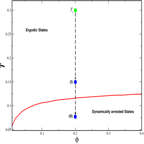
Figure 1: Dynamical arrest line (solid curve) in the ($\phi,T$) state space of the system of interacting dipoles with fixed positions. This line is the boundary between the region of ergodic states, at which the system is predicted to reach thermodynamic equilibrium, and the predicted region of dynamically arrested states. Each of the two superimposed vertical dashed arrows represent the quench of the system from an initial temperature $T_{i}$ (green dot) to a final temperature $T_{f}$ (blue dots), in one case above ($\mathbf{I}$) and in the other case below ($\mathbf{II}$) the dynamic arrest line.

We can now use the same thermodynamic function $\mathcal{E}_{lm}^{(f)}(k)\equiv\mathcal{E}_{lm}(k;\phi,T_{f})$ to go beyond the determination of the dynamic arrest line $T_{c}=T_{c}(\phi)$ by solving the set of NE-SCGLE equations (46)-(50) to describe the rotational diffusive relaxation of our system. For this, let us notice that these equations happen to have the same mathematical structure as the NE-SCGLE equations that describe the translational diffusion of spherical particles (see, e.g., Eqs. (2.1)-(2.6) of Ref. nescgle5 ). Although the physical meaning of these two sets of equations is totally different, their mathematical similarity allows us to implement the same method of solution described in Ref. nescgle3 . Thus, we do not provide further details of the numerical protocol to solve Eqs. (46)-(50), but go directly to illustrate the resulting scenario.

At this point let us notice that there are two possible classes of stationary solutions of Eq. (46). The first class corresponds to the long-time asymptotic condition $\lim_{t\to\infty}S_{lm}(k;t)=1/\mathcal{E}_{lm}^{(f)}(k)$, in which the system is able to reach the thermodynamic equilibrium condition $S_{lm}^{eq}(k)=1/\mathcal{E}_{lm}^{(f)}(k)$. Equilibration is thus a sufficient condition for the stationarity of $S_{lm}(k,t)$. It is, however, not a necessary condition. Instead, according to Eq. (46), another sufficient condition for stationarity is that $\lim_{t\to\infty}b_{R}(t)=0$. This is precisely the hallmark of dynamically-arrested states. In what follows we discuss the phenomenology predicted by the solution of Eqs. (46)-(50) for each of these two mutually exclusive possibilities.

IV.2 Equilibration of the system of interacting dipoles with random fixed positions.

Let us now discuss the solution of Eqs. (46)-(50) describing the non-equilibrium response of the system to an instantaneous temperature quench. For this, we assume that the system was prepared in an equilibrium state characterized by the initial value $S_{lm}^{(i)}(k)=S_{lm}^{(eq)}(k,\phi,T_{i})=S_{lm}(k,t=0)$, of $S_{lm}(k,t)$, and that at time $t=0$ the temperature is instantaneously quenched to a final value $T_{f}$. Normally one expects that, as a result, the system will eventually reach full thermodynamic equilibrium, so that the long time asymptotic limit of $S_{lm}(k,t)$ will be the equilibrium projections $S_{lm}^{(eq)}(k;\phi,T_{f})$. Such equilibration processes are illustrated in Fig. 2(a) with an example in which the system was quenched from an initial equilibrium state at temperature $T_{i}=0.3$, $S_{lm}(k,t=0)=S_{lm}(k;\phi,T_{i})$, to a final temperature $T_{f}=0.15>T_{c}=0.116$, keeping the volume fraction constant at $\phi=0.2$ (the first of the two quenches schematically indicated by the dashed vertical arrows of Fig. 1).

Under these conditions, and from the physical scenario predicted in Fig. 1, we should expect that the system will indeed equilibrate, so that $S_{lm}(k,t\to\infty)=S_{lm}^{(eq)}(k;\phi,T_{f})$. This, however, will only be true for $S_{10}(k,t)$ and $S_{11}(k,t)$, since, according to Eq. (46), $S_{00}(k,t)$ must remain constant for $t>0$, indicating that the artificially-quenched spatial structure will not evolve as a result of the temperature quench. For the same reason, Eqs. (47) and (48) imply that the normalized intermediate scattering functions $F_{00}(k,\tau;t)/S_{00}(k;t)$ and $F_{00}^{S}(k,\tau;t)$ will be unity for all positive values of the correlation time $\tau$ and waiting time $t$. For reference, the structure of the frozen positions represented by $S_{00}(k,t)=S_{00}^{(eq)}(k,\phi,T_{i})$, is displayed in Fig. 2(a) by the (magenta) dotted line, which clearly indicates that the fixed positions of the dipoles are strongly correlated, in contrast with a system of dipoles with purely random fixed positions, in which $S_{00}(k,t)$ would be unity. In the same figure, the initial and final equilibrium static structure factor projections, $S^{(i)}_{10}(k)=S_{10}^{(eq)}(k;\phi,T_{i})$ and $S^{(f)}_{10}(k)=S_{10}^{(eq)}(k;\phi,T_{f})$, are represented, respectively, by the (red) dashed and (blue) dot-dashed curves. The sequence of (brown) solid curves in between represents the evolution of $S_{10}(k,t)$ with waiting time $t$, as a series of snapshots corresponding to the indicated values of $t$.

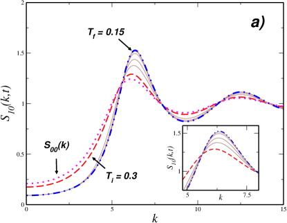
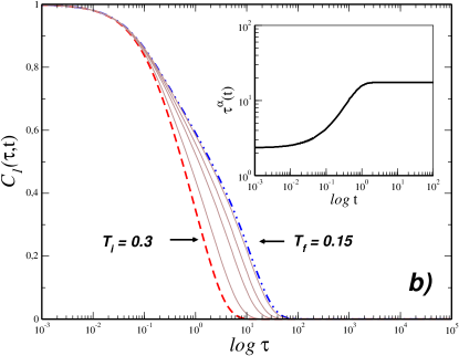
Figure 2: (Color online) Illustration of an equilibration process: (a) Snapshots of the time evolution of the $l=1,m=0$ static structure factor projection, $S_{10}(k,t)$, corresponding to the isochoric quench $T_{i}\to T_{f}$ for $\phi=0.2$, with $T_{i}=0.3$ and $T_{f}=0.15$. The (red) dashed line is the initial structure factor $S_{10}(k,t=0)=S_{10}^{(i)}(k)$. The (blue) dot-dashed line is the asymptotic limit $S_{10}(k,t\to\infty)=S_{10}^{(f)}(k)=S_{10}^{(eq)}(k)$. The sequence of thinner (brown) solid lines in between represents $S_{10}(k,t)$ for $t=0.3,\ 0.78,\ 1.42,\ 2.33\ \text{and}\ t\to\infty$. For reference we also include the non-evolving component $S_{00}(k,t)=S_{00}^{eq}(k;\phi,T_{i})$, indicated by the dotted line. (b) Snapshots of the orientational autocorrelation function $C_{1}(\tau;t)$ as a function of correlation time $\tau$ (thin brown solid lines), corresponding to the same isochoric quench and same sequence of waiting times $t$ as in (a). The (red) dashed line represents the initial function $C_{1}(\tau;t=0)=C^{(eq)}_{1}(\tau;\phi,T_{i})$ and the (blue) dot-dashed line is the asymptotic limit $C_{1}(\tau;t\to\infty)=C^{(eq)}_{1}(\tau;\phi,T_{f})$. The inset plots the $\alpha$-relaxation time, defined as $C_{1}(\tau_{\alpha};t)=1/e$, as a function of waiting time $t$.

For each snapshot of the static structure factor projections $S_{lm}(k,t)$, the solution of Eqs. (46)-(50) also determines a snapshot of each of the dynamic correlation functions $F_{lm}(k,\tau;t)$ and $F^{S}_{lm}(k,\tau;t)$. These functions are related with other more intuitive and experimentally accessible properties, such as the time-dependent autocorrelation function $C_{1}(\tau;t)\equiv\langle\sum_{i=1}^{N}\hat{\bm{\mu}}_{i}(t+\tau)\cdot\hat{\bm{\mu}}_{i}(t)\rangle/\langle\sum_{i=1}^{N}\hat{\bm{\mu}}_{i}(t)\cdot\hat{\bm{\mu}}_{i}(t)\rangle$ of the normalized dipole vectors $\hat{\bm{\mu}}_{i}$. In fact, since our dynamic correlators $F_{lm}(k,\tau;t)$ and $F^{S}_{lm}(k,\tau;t)$ were assumed to be described from the intermolecular $k$-frame gory1 , one can relate them with the time-dependent autocorrelation function $C_{1}(\tau;t)$ directly through the following expression fabbian1 ,

$$C_{1}(\tau;t)=\frac{1}{3}\lim_{k\to 0}\sum_{m=-1}^{1}F^{S}_{1m}(k,\tau;t)$$ (52)

Let us notice that, according to Eq. (48), the three terms in the sum on the right hand side of Eq. (52), $F^{S}_{10}(k,\tau;t),F^{S}_{11}(k,\tau;t)$ and $F^{S}_{1-1}(k,\tau;t)$, satisfy the same equation of motion (which only depends explicitly on $l$) and thus, contribute exactly in the same manner to the $\tau$ and $t$ dependence of $C_{1}(\tau;t)$. Thus, $C_{1}(\tau;t)$ summarizes the irreversible time evolution of the orientational dynamics, as illustrated in Fig. 2(b) with the snapshots corresponding to the same set of evolution times $t$ as the snapshots of $S_{10}(k,t)$ in Fig. 2(a). We observe that $C_{1}(\tau;t)$ starts from its initial equilibrium value, $C_{1}(\tau;t=0)=C^{(eq)}_{1}(\tau;\phi,T_{i})$ and quickly evolves with waiting time $t$ towards $C_{1}(\tau;t\to\infty)=C^{(eq)}_{1}(k,\tau;\phi,T_{f})$. This indicates that the expected equilibrium state at ($\phi=0.2,T_{f}$) is reached without impediment and that the orientational dynamics remains ergodic at that state point.

As mentioned before, the structure of Eqs. (46)-(50) is the same as that of the equations in nescgle3 describing the spherical case. Thus, one should not be surprised that the general dynamic and kinetic scenario predicted in both cases will exhibit quite similar patterns. For example, the non-equilibrium evolution described by the sequence of snapshots of $C_{1}(\tau;t)$ can be summarized by the evolution of its $\alpha$-relaxation time $\tau_{\alpha}(t)$, defined through the condition $C_{1}(\tau_{\alpha};t)=1/e$. In the inset of Fig. 2(b) we illustrate the saturation kinetics of the equilibration process in terms of the $t$-dependence of $\tau_{\alpha}(t)$, as determined from the sequence of snapshots of $C_{1}(\tau_{\alpha};t)$ displayed in the figure. Clearly, after a transient stage, in which $\tau_{\alpha}(t)$ evolves from its initial value $\tau_{\alpha}^{eq}(\phi,T_{i})$, it eventually saturates to its final equilibrium value $\tau_{\alpha}^{eq}(\phi,T_{f})$.

IV.3 Aging of the system of interacting dipoles with random fixed positions.

Let us now present the NE-SCGLE description of the second class of irreversible isochoric processes, in which the system starts in an ergodic state but ends in a dynamically arrested state. For this, let us consider now the case in which the system is subjected to a sudden isochoric cooling, at fixed volume fraction $\phi=0.2$, and from the same initial state as before, but this time to the final state point $(\phi,T_{f}=0.095)$ lying inside the region of dynamically arrested states (the second of the two quenches schematically indicated by the dashed vertical arrows of Fig. 1).

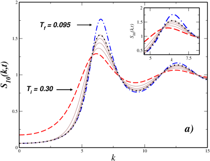
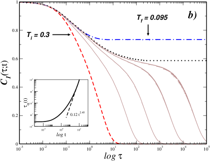
Figure 3: Illustration of an aging process: (a) Snapshots of the non-equilibrium time evolution of the $l=1,m=0$ static structure factor projection, $S_{10}(k,t)$, corresponding to the isochoric quench $T_{i}\to T_{f}$ for $\phi=0.2$, with $T_{i}=0.3$ and $T_{f}=0.095$. The (red) dashed line is the initial structure factor $S_{10}(k,t=0)=S_{10}^{(i)}(k)$. The (blue) dot-dashed line is the (now inaccessible) equilibrium structure factor $S_{10}^{(eq)}(k;\phi,T_{f})$, whereas the (black) dotted line is the predicted asymptotic limit $S_{10}(k,t\to\infty)=S_{10}^{(a)}(k)$. The sequence of thinner (brown) solid lines in between represents $S_{10}(k,t)$ for $t=1.16,\ 4.264,\ 14.056,\ \text{and}\ 150.61$. (b) Snapshots of the orientational autocorrelation function $C_{1}(\tau;t)$ as a function of correlation time $\tau$ (thin brown solid lines), corresponding to the same isochoric quench and same sequence of waiting times $t$ as in (a). The (red) dashed line represents the initial function $C_{1}(\tau;t=0)=C^{(eq)}_{1}(\tau;\phi,T_{i})$, the (blue) dot-dashed line is the expected (but now inaccessible) equilibrium correlation $C^{(eq)}_{1}(\tau;\phi,T_{f})$, and the (black) dotted line is the predicted long-$t$ asymptotic limit, $C_{1}(\tau;t\to\infty)=C^{(a)}_{1}(\tau)$. The inset plots the corresponding $\alpha$-relaxation time as a function of waiting time $t$, with the (black) dashed line representing the asymptotic power law $\tau_{\alpha}\propto t^{2.45}$.

Under such conditions, the long-time asymptotic limit of $S_{lm}(k;t)$ will no longer be the expected equilibrium static structure factor $S^{(eq)}_{lm}(k;\phi,T_{f})$, but another, well-defined non-stationary structure factor $S^{(a)}_{lm}(k)$. In Fig. 3(a) we illustrate this behavior with a sequence of snapshots of the non-equilibrium evolution of $S_{10}(k;t)$ after this isochoric quench at $\phi=0.2$ from $T^{(i)}=0.3$ to $T^{(f)}=0.095$. There we highlight the initial structure factor $S_{10}^{(i)}(k)=S_{10}^{(eq)}(k;\phi,T_{i})$, represented by the (red) dashed line and the dynamically arrested long-time asymptotic limit, $S^{(a)}_{10}(k)$, of the non-equilibrium evolution of $S_{10}(k;t)$, described by the (black) dotted line. For reference, we also plot the expected, but inaccessible, equilibrium static structure factor $S^{(eq)}_{10}(k;\phi,T_{f})\neq S^{(a)}_{10}(k)$ (blue dot-dashed line).

Finally, let us illustrate how this scenario of dynamic arrest manifests itself in the non-equilibrium evolution of the dynamics. We recall that for each snapshot of the non-stationary structure factor $S_{lm}(k;t)$, the solution of Eqs. (46)-(50) also determines a snapshot of all the dynamic properties at that waiting time $t$. For example, in Fig. 3(b) we present the sequence of snapshots of $C_{1}(\tau;t)$, plotted as a function of correlation time $\tau$, that corresponds to the sequence of snapshots of $S_{10}(k;t)$ in Fig 3(a). In this figure we highlight in particular the initial value $C_{1}(\tau;t=0)=C^{(eq)}_{1}(\tau;\phi,T_{i})$ (red dashed line), the predicted non-equilibrium asymptotic limit, $C^{(a)}_{1}(\tau)\equiv\lim_{t\rightarrow\infty}C_{1}(k,\tau;t)$ (black dotted line) and the inaccessible equilibrium value of $C^{(eq)}_{1}(\tau;\phi,T_{f})$ (blue dot-dashed line). Notice that, in contrast with the equilibration process, in which the long-time asymptotic solution $C^{(eq)}_{1}(\tau;\phi,T_{f})$ decays to zero within a finite relaxation time $\tau_{\alpha}^{eq}(\phi,T_{f})$, in the present case $C^{(eq)}_{1}(\tau;\phi,T_{f})$ does not decay to zero, but to a finite plateau. This arrested equilibrium correlation function, however, is completely inaccessible, since now the long-$t$ asymptotic limit of $C_{1}(k,\tau;t)$ is $C^{(a)}_{1}(\tau)$, which is also a dynamically arrested function, but with a different plateau than $C^{(eq)}_{1}(\tau;\phi,T_{f})$.

Just like in the equilibration process, which starts at the same initial state, here we also observe that at $t=0$, $C_{1}(\tau;t)$ shows no trace of dynamic arrest, and that as the waiting time $t$ increases, the relaxation time increases as well. We can summarize this irreversible evolution of $C_{1}(\tau;t)$ by exhibiting the kinetics of the $\alpha$-relaxation time $\tau_{\alpha}(t)$ extracted from the sequence of snapshots of $C_{1}(\tau_{\alpha};t)$ in the same figure. This is done in the inset of fig. 3(b). Clearly, after the initial transient stage, in which $\tau_{\alpha}(t)$ increases from its initial value $\tau_{\alpha}^{eq}(\phi,T_{i})$ in a similar fashion as in the equilibration case, $\tau_{\alpha}(t)$ no longer saturates to any finite stationary value. Instead, it increases with $t$ without bound, and actually diverges as a power law, $\tau_{\alpha}(t)\propto t^{a}$, with $a\approx 2.45$.

Except for quantitative details, such as the specific value of this exponent, we find a remarkable general similarity between this predicted aging scenario of the dynamic arrest of our system of interacting dipoles, and the corresponding aging scenario of the structural relaxation of a soft-sphere glass-forming liquid described in Ref. nescgle3 (compare, for example, our Fig. 3(b) above, with Fig. 12 of that reference). As said above, however, our intention in this paper is not to discuss the physics behind these similarities and these scenarios, but only to present the theoretical machinery that reveals it.

V Conclusions

Thus, in summary, we have proposed the extension of the self-consistent generalized Langevin equation theory for systems of non-spherical interacting particles (NS-SCGLE), to consider general non-equilibrium conditions. The main contribution of this work consist thus in the general theoretical framework, developed in Sec. III, able to describe the irreversible processes occurring in a given system after a sudden temperature quench, in which its spontaneous evolution in search of a thermodynamic equilibrium state could be interrupted by the appearance of conditions of dynamical arrest for translational or orientational (or both) degrees of freedom.

Our description consists essentially of the coarse-grained time-evolution equations for the spherical-harmonics-projections of the static structure factor of the fluid, which involves one translational and one orientational time-dependent mobility functions. These non-equilibrium mobilities, in turn, are determined from the solution of the non-equilibrium version of the SCGLE equations for the non-stationary dynamic properties (the spherical-harmonics-projections of the self and collective intermediate scattering functions). The resulting theory is summarized by Eqs. (39)-(45) which describe the irreversible processes in model liquids of non-spherical particles, within the constraint that the system remains, on the average, spatially uniform. This theoretical framework is now ready to be applied for the description of such nonequilibrium phenomena in many specific model systems.

Although in this paper we do not include a thorough discussion of any particular application, in section IV we illustrated the predictive capability of our resulting equations by applying them to the description of the isochoric and uniform evolution of non-equilibrium process of a simple model, namely, a dipolar hard sphere liquid with fixed random positions, after being subjected to instantaneous temperature quench. Here we used this example mostly to illustrate some methodological aspects of the application of the theory, since this specific application allows us to easily implement the numerical methods described in detail in Ref. nescgle3 . The same illustrative example, however, also allows us to investigate the relevant features of the orientational dynamics during the equilibration and aging processes, but leaves open many relevant issues, such as the relationship between these predictions and the phenomenology of aging in spin-glass systems. Similarly, the non-equilibrium manifestations of the coupling between translational and rotational dynamics, involved in the complete solution of Eqs. (39)-(45), will be the subject of future communications. Thus, we expect that the general results derived in this paper will be the basis of a rich program of research dealing with these problems.

References

- (1) Angell C. A., Ngai K. L., McKenna G. B., McMillan P. F. and Martin S. F., J. Appl. Phys. 88 3113 (2000).
- (2) K. L. Ngai, D. Prevosto, S. Capaccioli and C. M. Roland, J. Phys.: Condens. Matter 20, 244125 (2008)
- (3) F. Sciortino and P. Tartaglia, Adv. Phys. 54, 471 (2005).
- (4) J. A. Mydosh, Spin Glasses: An Experimental Introduction (Taylor Francis, London, 1993).
- (5) Ka-Ming Tam and M.J.P. Gingras, Phys. Rev. Lett., 103, 087202 (2009).
- (6) A. Biltmo and P. Henelius, Nat. Commun. 3:857 (2012).
- (7) J. Keizer, Statistical Thermodynamics of Nonequilibrium Processes, Springer-Verlag (1987).
- (8) S. R. de Groot and P. Mazur Non-equlibrium Thermodynamics, Dover, New York (1984).
- (9) G. Lebon, D. Jou, and J. Casas-Vázquez, Understanding Non-equilibrium Thermodynamics Foundations, Applications, Frontiers, Springer-Verlag Berlin Heidelberg (2008).
- (10) W. Götze, in Liquids, Freezing and Glass Transition, edited by J. P. Hansen, D. Levesque, and J. Zinn-Justin (North-Holland, Amsterdam, 1991).
- (11) W. Götze and L. Sjögren, Rep. Prog. Phys. 55, 241 (1992).
- (12) L. Yeomans-Reyna et al., Phys. Rev. E 76, 041504 (2007).
- (13) R. Juárez-Maldonado et al., Phys. Rev. E 76, 062502 (2007).
- (14) A. Latz, J. Phys.: Condens. Matter, 12 (2000) 6353.
- (15) P. E. Ramírez-González and M. Medina-Noyola, Phys. Rev. E 82, 061503 (2010).
- (16) P. E. Ramírez-González and M. Medina-Noyola, Phys. Rev. E 82, 061504 (2010).
- (17) L. Onsager, Phys. Rev. 37, 405 (1931).
- (18) L. Onsager, Phys. Rev. 38, 2265 (1931).
- (19) L. Onsager and S. Machlup, Phys. Rev. 91, 1505 (1953).
- (20) S. Machlup and L. Onsager, Phys. Rev. 91, 1512 (1953).
- (21) M. Medina-Noyola, Faraday Discuss. Chem. Soc.(1987), 83, 21-31
- (22) M. Medina-Noyola and J.L. del Río Correa, Physica 146A, (1987) 483-505
- (23) L. E. Sánchez-Díaz, P. E. Ramírez-González and M. Medina-Noyola, Phys. Rev. E 87, 052306 (2013).
- (24) P. Mendoza-Méndez, E. Lázaro-Lázaro, L. E. Sánchez-Díaz, P. E. Ramírez-González, G. Pérez-Ángel, and M. Medina-Noyola, PRL, Sumitted (2016); arXiv:1404.1964
- (25) J. M. Olais-Govea, L. López-Flores, and M. Medina-Noyola, J. Chem Phys. 143, 174505 (2015).
- (26) J. M. Olais-Govea, L. López-Flores, and M. Medina-Noyola, PRL, Sumitted (2016); arXiv:1505.00390
- (27) L. E. Sánchez-Díaz, E. Lázaro-Lázaro, J. M. Olais-Govea and M. Medina-Noyola, J. Chem Phys. 140, 234501 (2014).
- (28) J. W. Cahn and J. E. Hilliard, J. chem. Phys. 31, 688 (1959).
- (29) H. E. Cook, Acta Metall. 18, 297 (1970).
- (30) H. Furukawa, Adv. Phys., 34, 703 (1985).
- (31) P. J. Lu, E. Zaccarelli, F. Ciulla, A. B. Schofield, F. Sciortino and D. Weitz, Nature 22, 499 (2008).
- (32) E. Sanz, M. E. Leunissen, A. Fortini, A. van Blaaderen, and M. Dijkstra, J. Phys. Chem. B 112, 10861 (2008).
- (33) T. Gibaud and P. Schurtenberger, J. Phys.: Condens. Matter 21, 322201 (2009).
- (34) L. Di Michele, D. Fiocco, F. Varrato, S. Sastry, E. Eisera and G. Foffi, Soft Matter 10, 3633 (2014).
- (35) Y. Gao, J. Kim, and M. E. Helgeson, Soft Matter, 11, 6360-6370 (2015).
- (36) E. Zaccarelli, J. Phys.: Condens. Matter 19, 323101 (2007).
- (37) J. F. M. Lodge and D. M. Heyes, J. Chem. Soc., Faraday Trans., 93, 437 (1997).
- (38) W. Kob and H. C. Andersen, Phys. Rev. Lett. 73, 1376 (1994); Phys. Rev. E 51, 4626 (1995); 52, 4134 (1995).
- (39) V. Testard, L. Berthier, and W. Kob, J. Chem. Phys. 140, 164502 (2014).
- (40) L. Berthier and G. Biroli, Rev. Mod. Phys. 83 (2011).
- (41) E. Sanz, M. E. Leunissen, A. Fortini, A. van BLaaderen, and M. Dijkstra, J. Phys. Chem. B, 112, 10861 (2008).
- (42) K. N. Pham, S. U. Egelhaaf, P. N. Pusey, and W. C. K. Poon, Phys. Rev. E 69, 011503 (2004).
- (43) L. Cipelletti and L. Ramos, J. Phys.: Condens. Matter 17, 253, 285 (2005).
- (44) V. A. Martinez, G. Bryant, and W. van Megen, Phys. Rev. Lett. 101, 135702 (2008).
- (45) P. J. Lu et al., Nature 453: 499 (2008).
- (46) Z. Zheng, F. Wang and Y. Han, Phys. Rev. Lett. 107, 065702 (2011).
- (47) K.V.Edmond, M. T. Elsesser, G.L. Hunter, D.J. Pine and E.R. Weeks (2012), Proc. Natl. Acad. Sci. USA, 109: 17891-17896.
- (48) L.F. Elizondo-Aguilera, P. F. Zubieta-Rico, H. Ruíz Estrada, and O. Alarcón-Waess, Phys. Rev. E, 90, 052301 (2014).
- (49) R. Schilling and T. Scheidsteger, Phys. Rev. E, 56, No.3, 2932 (1997).
- (50) L. Fabbian, et.al., Phys. Rev. E, 60, No.5, 5768 (1999).
- (51) M. Letz, R. Schilling and A. Latz, Phys. Rev. E, 62, No.4, 5173 (2000).
- (52) H. Callen, Thermodynamics, John Wiley, New York(1960).
- (53) M. S. Wertheim, J. Chem. Phys. 55, 4291 (1971).
- (54) L. Fabbian, F. Sciortino and P. Tartaglia, J. of Non-Cryst. Solids 235-237 (1998) 325-330