From geometric optics to plants: eikonal equation for buckling

Sergei Nechaev^∗a,b and Kirill Polovnikov,^c

Received Xth XXXXXXXXXX 20XX, Accepted Xth XXXXXXXXX 20XX
First published on the web Xth XXXXXXXXXX 200X

DOI: 10.1039/b000000x

Optimal embedding in the three-dimensional space of exponentially growing squeezed surfaces, like plants leaves, or 2D colonies of exponentially reproducing cells, is considered in the framework of conformal approach. It is shown that the boundary profile of a growing tissue is described by the 2D eikonal equation, which provides the geometric optic approximation for the wave front propagating in the media with inhomogeneous refraction coefficient. The variety of optimal surfaces embedded in 3D is controlled by spatial dependence of the refraction coefficient which, in turn, is dictated by the local growth protocol.

1 Introduction

Variety of shapes of 2D growing tissues emerges due to the incompatibility of local internal (differential) growth protocol with geometric constraints imposed by embedding of these tissues into the space. For example, buckling of a lettuce leaf can be naively explained as a conflict between natural growth due to the periphery cells division (typically, exponential), and growth of circumference of a planar disc with gradually increasing radius. Due to a specific biological mechanism which inhibits growth of the cell experiencing sufficient external pressure, the division of inner cells is insignificant, while periphery cells have less steric restrictions and proliferate easier. Thus, the division of border cells has the major impact on the instabilities in the tissue. Such a differential growth induces an increasing strain in a tissue near its edge and results in two complimentary possibilities: i) in-plane tissue compression and/or redistribution of layer cells accompanied by the in-plane circumference instability, or ii) out-of-plane tissue buckling with the formation of saddle-like surface regions. The latter is typical for various undulant negatively curved shapes which are ubiquitous to many mild plants growing up in air or water where the gravity is of sufficiently small matter ^{1, 13}.

A widely used energetic approach to growing patterns exploits a continuous formulation of the differential growth and is based on a rivalry between bending and stretching energies of elastic membranes ^{10, 6, 15, 7, 13, 14, 19, 18}, reflecting the choice between options (i) and (ii) above. For bending rigidity of a thin membrane, ${\cal B}$, one has ${\cal B}\sim h^{3}$, while stretching rigidity, ${\cal S}$ behaves as ${\cal S}\sim h$, where $h$ is the membrane thickness ⁸. Therefore, thin enough tissues, with $h\ll 1$, prefer to bend, i.e. to be negatively curved under relatively small critical strain.

The latter allows one to eliminate the ”stretching” regime from consideration, justifying the geometric approach for infinitesimally thin membranes ^{3, 4, 12, 16, 17, 7} (see also ⁵). Here the determination of typical profiles of buckling surfaces relies on an appropriate choice of metric tensor of the non-Euclidean space, and is realized via the optimal embedding of the tissue with certain metrics into the 3D Euclidean space. It should be mentioned, that the formation of wrinkles within this approach seems to be closely related to the description of phyllotaxis via conformal methods ²⁰.

In this letter we suggest a model of a hyperbolic infinitesimally thin tissue, whose periphery cells divide freely with exponential rate, while division of inner cells is absolutely inhibited. Two cases of proliferations, the one-dimensional (directed) and the uniform two-dimensional, are considered. The selection of these two growth models is caused by the intention to describe different symmetries inherent for plants at initial stages of growth. As long as the in-plane deformations are not beneficial, as follows from the relationship between bending and stretching rigidities, all the redundant material of fairly elastic tissue will buckle out. In order to take into account the finite elasticity of growing tissue, resulting from the intrinsic discrete properties of a material, we describe the tissue as a collection of glued elementary plaquettes connected along the hyperbolic graph, $\gamma$. The discretization implies the presence of a characteristic scale, of order of the elementary cell (plaquette) size, below which the tissue is locally flat.

As we rely on the absence of in-plane deformations, this graph has to be isometrically embedded into the 3D space. The desired smooth surface profile is obtained in two steps: i) isometric mapping of the hyperbolic graph onto the flat domain (rectangular or circular) with hyperbolic metrics, ii) subsequent restoring of the metrics into the 3D Euclidean space above the domain. We demonstrate that such a procedure leads to the ”optimal” buckling of the tissue and is described by the eikonal equation for the profile, $f(x,y)$, of growing sample, which by definition, is a variant of the Hamilton-Jacobi equation.

The paper is organized as follows. We introduce necessary definitions in the Section 2.1; the model under consideration and the details of the conformal approach are provided in the Sections 2.2, 2.3 and Appendix; the samples of various typical shapes for two-dimensional uniform and for one-dimensional directed growth, are presented in the Section 3; finally, the results of the work are summarized in the Section 4, where we also speculate about possible generalizations and rise open questions.

2 Buckling of thin tissues in cylindric and planar geometries

2.1 Basic facts about the eikonal equation

To make the content of the paper as self-contained as possible, it seems instructive to provide some important definitions used at length of the paper. The key ingredient of our consideration is the ”eikonal” equation, which is the analogue of the Hamilton-Jacobi equation in geometric optics. As we show below, the eikonal equation provides optimal embedding of an exponentially growing surface into the 3D Euclidean plane. Meaning of the notion ”optimal” has two different connotations in our approach:

i) On one hand, from viewpoint of the Hamilton-Jacobi theory, the eikonal equation appears in the minimization of the action $A=\int_{\gamma}Ldt$ with some Lagrangian $L$. According to the Fermat principle, the time of the ray propagation in the inhomogeneous media with the space-dependent refraction coefficient, $n(x,y)$, should be minimal.

ii) On the other hand, the eikonal equation emerges in our work in a purely geometric setting following directly from the conformal approach.

First attempts to formulate classical mechanics problems in geometric optics terms goes back to the works of Klein ²⁴ in 19th century. His ideas contributed to the corpuscular theory in a short-wavelength regime, as long as the same mechanical formalism applied to massless particles, was consistent with the wave approach. Later, in the context of general relativity, this approach was renewed to treat gravitational field as an optic medium ²⁵.

The Fermat principle states that the time $dt$ for a ray to propagate along a curve $\gamma$ between two closely located points $M({\bf x})$ and $N({\bf x}+d{\bf x})$ in an inhomogeneous media, should be minimal. The total time $T$ can be written in the form $T=\frac{1}{c}\int_{M}^{N}n(\mathbf{x}(s))ds$ where $n(\mathbf{x})=\frac{c}{\textrm{v}(\mathbf{x})}$ is the refraction coefficient at the point $\mathbf{x}=\{x^{i}\}$ of a $D$-dimensional space $(i=1,...,D)$, $c$ and $\textrm{v}(\mathbf{x})$ are correspondingly the light speeds in vacuum and in the media, and $d|\mathbf{x}|=ds$ is the spatial increment along the ray. Following the optical-mechanical analogy, according to which the action in mechanics corresponds to eikonal in optics, one can write down the ”optic length” or eikonal, $S=cT$ in Lagrangian terms: $S=\int_{M}^{N}L(\mathbf{x},\dot{\mathbf{x}})ds$ with the Lagrangian $L(\mathbf{x},\dot{\mathbf{x}})=n(\mathbf{x}(s))\sqrt{\dot{\mathbf{x}}(s)\dot{\mathbf{x}}(s)}$, where $\dot{\mathbf{x}}^{2}=\sum_{i=1}^{D}\big{(}\frac{dx^{i}}{ds}\big{)}^{2}$. We would like to mention here, that optical properties of the media can be also treated in terms of induced Riemann metrics in vacuum:

$$S=\int_{M}^{N}n(\mathbf{x}(s))ds=\int_{M}^{N}\sqrt{\dot{\mathbf{x}}g(\mathbf{x})\dot{\mathbf{x}}}ds$$ (1)

where $g_{ij}=n^{2}(\mathbf{x})\delta_{ij}$ stands for induced metrics components in isotropic media case. Thus, from the geometrical point, the ray trajectory can be understood as a ”minimal curve” in a certain Riemann space. This representation suggests to consider optimal ray paths as geodesics in the space with known metrics $g$.

Stationarity of optic length, $S$, i.e. $\delta S=0$, together with the condition $|\dot{\mathbf{x}}|=1$, defines the Euler equation:

$$\frac{d}{ds}\left(n(\mathbf{x})\frac{d\mathbf{x}}{ds}\right)=\nabla n(\mathbf{x})$$ (2)

from which one can directly proceed to the Huygens principle by integrating (2) over $s$: $\nabla S(\mathbf{x})=n(\mathbf{x})\frac{d\mathbf{x}}{ds}$. Squaring both sides of the latter equation we end up with the eikonal equation:

$$\left(\nabla S(\mathbf{x})\right)^{2}=n^{2}(\mathbf{x})$$ (3)

The eikonal equation Eq.(3) has the same form as the Hamilton-Jacobi equation in mechanics for action in the $D+1$-dimensional space, which in turn can be understood as the relativistic equation for the light, propagating in the Riemannian space.

2.2 The model: formalization of physical ideas

In our work the eikonal equation arises in the differential growth problem in a purely geometric setting. Consider a tissue, represented by a colony of cells, growing in space without any geometric constraints. The local division protocol is prescribed by nature, being particularly recorded in genes and is accompanied by their mutations ¹¹. The exponential cell division is implied, as already mentioned above. To make our viewpoint more transparent, suppose that all cells, represented by equilateral triangles, divide independently and their proliferation is initiated by the first ”protocell”. Connecting the centers of neighboring triangles by nodes, we rise a graph $\gamma$. The number of vertices, $P_{\gamma}(k)$, in the generation $k$, grows exponentially with $k$: $P_{\gamma}(k)\sim c^{k}$ ($c>1$). It is known that exponential graphs possess hyperbolic metrics, meaning that they can be isometrically (with fixed branch lengths and angles between adjacent branches) embedded into a hyperbolic plane. Thus, it is clear, that the corresponding surface, pulled on the isometry of such graph in the 3D Euclidean space, should be negatively curved.

To have a relevant image, suppose that we grow the surface by crocheting it spirally starting from the center ². Demanding two nearest neighboring circumference layers, $P(r)$ and $P(r+\Delta r)$, to differ by a factor of $c$ (where $c=\mathrm{const}>1$), i.e., $P(r+\Delta r)/P(r)=c$, we construct an exponentially growing (hyperbolic) surface – see the Fig.1a known as Amsler surface ³¹. The crocheted surface has well-posed properties on large scales, but should be precisely described on the scale of order of the elementary cell. As we have mentioned, the microscopic description is connected with the specific local growth protocol. The simplest way to generate the discrete hyperbolic-like surface out of equilateral triangles, consists in gluing 7 such triangles in each graph vertex and construct a piecewise surface, shown in the Fig.1b. On the scale less than the elementary cell $ABC$ this surface is flat. Thus, the size $a$ ($|AB|=|AC|=|BC|=a$) of the triangle $ABC$ stands for the rigidity parameter, playing the role of a characteristic scale in our problem, below which no deviations from the Euclidean metrics can be found. Later on we shall see that buckling of growing surface essentially depends on this parameter.

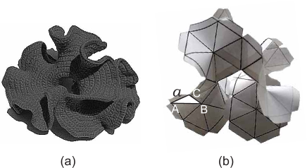
Fig.  1: (a) Hyperbolic surface obtained by spiral crocheting from the center; (b) Hyperbolic piecewise surface constructed by joining 7 equilateral flat triangles (copies of the triangle $ABC$) in each vertex. The triangle $ABC$ is lying in $z=x+iy$ plane in the 3D Euclidean space, $|AB|=|AC|=|BC|=a$.

We discuss buckling phenomena for two different growth symmetries shown schematically in the Fig.2a-b: i) uniform two-dimensional division from the point-like source (Fig.2a), and ii) directed one-dimensional growth from the linear segment (Fig.2b). In Fig.2a-b different generations of cells are shown by the shades of gray. For convenience of perception, sizes of cells in each new generation are decreasing in geometric progression, otherwise it would be impossible to draw them in a 2D flat sheet of paper and the figure would be incomprehensible. In Figs. 2c,d we imitate the protocols of growth depicted above in Figs. 2a,b by embedding the exponentially growing structure in the corresponding plane domain equipped with the hyperbolic metrics. The advantage of such embedding consists in the possibility to continue all functions smoothly through the boundaries of elementary domains, that cover the whole plane without gaps and intersections. Details of this construction and its connection to the growth in the 3D Euclidean space are explained below.

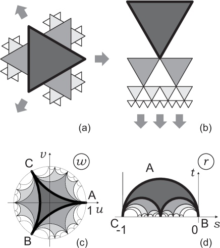
Fig.  2: (a) Uniform two-dimensional hyperbolic growth out of the unit domain in the plane; (b) One-dimensional hyperbolic growth out of the linear segment; c) Tessellation of the hyperbolic Poincaré disc by the images of flat Euclidean triangles; d) Tessellation of the domain in the hyperbolic half-plane by the images of flat Euclidean triangles.

It is known (see, for example ¹²) that the optimal buckling surface is fully determined by the metric tensor through the minimization of the discrete functional of special energetic form. Namely, define the energy of a deformed thin membrane, having buckling profile $f(x,y)$ above the domain, parameterized by $(x,y)$, as:

$$E\{f(x,y)\}\sim\sum_{i,j}\left(\Big{(}f_{ij}\Big{)}^{2}-\sum_{\alpha,\beta}\Delta^{\alpha}_{ij}g_{\alpha\beta}\Delta^{\beta}_{ij}\right)^{2}$$ (4)

where $g_{\alpha\beta}$ is the induced metrics of the membrane, $f_{ij}\equiv|f(x_{i},y_{i})-f(x_{j},y_{j})|$ is the distance between neighboring points and $\Delta_{ij}$ is the equilibrium distance between them. The typical (optimal) shape $\bar{f}(x,y)$ is obtained by minimization of (4) for any rigidity. However, the metric tensor, $g_{\alpha\beta}$ is a priori unknown since its elements depend on specifics of the differential growth protocol, therefore some plausible conjectures concerning its structure should be suggested. For example, in ¹² a directed growth of a tissue with one non-Euclidean metrics component, $g_{xx}(y)$, was considered. The diagonal component $g_{xx}(y)$ was supposed to increase exponentially in the direction of the growth, $y$, and crumpling of a leaf near its edge was finally established and analyzed.

2.3 Conformal approach

The preset rules of uniform exponential cells division determine the structure of the hyperbolic graph, $\gamma$, while the infinitesimal membrane thickness allows for the isometrical embedding of the graph $\gamma$ into the 3D space. We exploit conformal and metric relations between the surface structure in the 3D space and the graph $\gamma$ embedded into the flat domain with the hyperbolic metrics. The embedding procedure consists of a sequence of conformal transformations with a constraint on area preservation of an elementary plaquette. This eventually yields the knowledge of the Jacobian (the ”coefficient of deformation”), $J(x,y)$, for the hyperbolic surface, which is embedded into the 3D space via the orthogonal projection. Equipped by the key assumption, that a smooth yet unknown surface $f(x,y)$ is function, our procedure straightforwardly implies a differential equation on the optimal surface. Note that a version of the Amsler surface cannot be reconstructed in the same way since it is not a function above some planar domain.

To realize our construction explicitly, we first embed isometrically the graph $\gamma$: i) into the Poincaré disk ($|w|<1$) for the model of uniform planar growth, and ii) into the strip of the half-plane ($\textrm{Im}\,r>0,-1<\textrm{Re}\,r<0$) for the model of one-dimensional growth. In the Fig.3 we have drawn the tessellation of the Poincaré disc and of the strip by equilateral curvilinear triangles, which are obtained from the flat triangle $ABC$ of the hyperbolic surface (see Fig.1b) by conformal mappings $z(w)$ and $z(r)$ discussed below. Note, that a conformal mapping preserves the angles between adjacent branches of the graph. The graph $\gamma$, shown in the Fig.3, connects the centers of the triangles and is isometrically embedded into the corresponding hyperbolic domain. Besides, the areas of images of the domain ABC are the same.

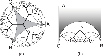
Fig.  3: Tessellation of the hyperbolic plane by the images of the curvilinear triangle $ABC$: (a) for Poincaré disc; (b) for a strip of the upper half-plane. The graph $\gamma$ connects the centers of images of $ABC$.

For the sake of definiteness consider the graph $\gamma$, isometrically embedded into the hyperbolic disk, shown in the Fig.3a. Now, we would like to find the surface in the 3D Euclidean space above the $w$-plane such that its Euclidean metrics coincides with the non-Euclidean metrics in the disk. The Hilbert theorem ³² prohibits to do that for the class of $C^{2}$-smooth surfaces. However, since we are interested in the isometric embedding of piecewise surface consisting of glued triangles of fixed area, we can proceed with the standard arguments of differential geometry ³³. The metrics $ds^{2}$ of a 2D surface, parameterized by $(u,v)$, is given by the coefficients

$$E=\mathbf{r}_{u}^{2},\quad F=\mathbf{r}_{v}^{2},\quad G=(\mathbf{r}_{u},\mathbf{r}_{v})$$ (5)

of the first quadratic form of this surface:

$$ds^{2}=E\,du^{2}+2F\,dudv+G\,dv^{2}$$ (6)

The surface area then reads $dS=\sqrt{EG-F^{2}}\,dudv$.

The area $S_{ABC}$ of the planar triangle $ABC$ on the plane $z=x+iy$ can be written as:

$$S_{ABC}=\int\limits_{\triangle ABC}dxdy=\mathrm{const}$$ (7)

where the integration is restricted by the boundary of the triangle. Since we aimed to conserve the metrics, let us require that the area of the hyperbolic triangle $ABC$, after the conformal mapping, is not changed and, therefore, it reads:

$$S_{ABC}=\int\limits_{\triangle ABC}|J(z,w)|dudv;\quad J(z,w)=\left|\begin{array}[]{cc}\displaystyle\partial_{u}x&\displaystyle\partial_{u}y\vskip 6.0pt plus 2.0pt minus 2.0pt\\ \displaystyle\partial_{v}x&\displaystyle\partial_{v}y\end{array}\right|$$ (8)

where $J(z,w)$ is the Jacobian of transition form $z$ to new coordinates, $w$. If $z(w)$ is holomorphic function, the Cauchy-Riemann conditions allow to write

$$J(w)=\left|\frac{dz(w)}{dw}\right|^{2}\equiv|z^{\prime}(w)|^{2}.$$ (9)

From the other hand, we may treat the value of the Jacobian, $J(w)$, as a factor relating the change of the surface element under transition to a new metrics, the co-called ”coefficient of deformation”. As long as the metrics in the hyperbolic domain should reproduce the Euclidean metrics of the smooth surface, $f(u,v)$, one should set $J=\sqrt{EG-F^{2}}$, where $E,G,F$ are the coefficients of the first quadratic form of the surface $f$. Now, if $f(u,v)$ is function above $w$-plane, its Jacobian adopts a simple form:

$$J(u,v)=\sqrt{1+(\partial_{u}f)^{2}+(\partial_{v}f)^{2}}$$ (10)

Making use of the polar coordinates in our complex $w$-domain, $\{(\rho,\phi):u=\rho\cos\phi,v=\rho\sin\phi\}$, we eventually arrive at nonlinear partial differential equation for surface profile $f(\rho,\phi)$ in the polar coordinates above $w$:

$$\Big{(}\partial_{\rho}f(\rho,\phi)\Big{)}^{2}+\frac{1}{\rho^{2}}\Big{(}\partial_{\phi}f(\rho,\phi)\Big{)}^{2}=|z^{\prime}(w)|^{4}-1$$ (11)

In the case of the hyperbolic strip domain, Fig.3b, the equation for the growth profile above the domain can be written in local cartesian coordinates, $r=s+it$:

$$\Big{(}\partial_{s}f(s,t)\Big{)}^{2}+\Big{(}\partial_{t}f(s,t)\Big{)}^{2}=|z^{\prime}(r)|^{4}-1$$ (12)

Note, that the inequalities $|z^{\prime}(w)|>1,|z^{\prime}(r)|>1$, following from (11)-(12), determine the local condition of existence of non-zero real solution and, as we discuss below, can be interpreted as the presence of a finite scale surface rigidity.

To establish a bridge between optic and growth problems, let us mention that, say, equation (11), coincides with the two-dimensional eikonal equation (3) for the wavefront, $S(w)$, describing the light propagating according the Huygens principle in the unit disk with the refraction coefficient

$$n(w)=\sqrt{|z^{\prime}(w)|^{4}-1}$$ (13)

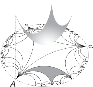
Fig.  4: Orthogonal projection above the Poincaré disc: area of the curvilinear triangle in Euclidean space coincides with the area of the triangle in hyperbolic metrics in Poincaré disc.

We can construct the conformal mappings $z(r)$ and $z(w)$ of the flat equilateral triangle $ABC$ in the Euclidean complex plane $z=x+iy$ onto the circular triangle $ABC$ in the complex domains $r=s+it$ and $w=\rho(\cos\phi+i\sin\phi)$ correspondingly. The absolute value of the Gaussian curvature is controlled by the number, $V$, of equilateral triangles glued in one vertex: the surface is hyperbolic only for $V>6$. The surfaces with any $V>6$ have qualitatively similar behavior, however the simplest case for analytical treatment corresponds to $V=\infty$, when the dual graph $\gamma$ is loopless. The details of the conformal mapping of the flat triangle with side $a$ to the triangle with angles $\{0,0,0\}$ in the unit strip $r$ are given in the Appendix. The Jacobian $J(z(r))$ of conformal mapping $z\to r$ reads:

$$J(r)=|z^{\prime}(r)|^{2}=\frac{h^{2}}{a^{2}}|\eta(r)|^{8}$$ (14)

and the Jacobian of the mapping $z\to w$, is written through the function $r(w)$ that conformally maps the triangle from the strip onto the Pincaré disk:

$$J(w)=|z^{\prime}(w)|^{2}=\frac{3h^{2}}{a^{2}}\frac{|\eta(r(w))|^{8}}{|1-w|^{4}}$$ (15)

where

$$r(w)=e^{-i\pi/3}\frac{e^{2i\pi/3}-w}{1-w}-1;\quad h=\left(\frac{16}{\pi}\right)^{1/3}\frac{\Gamma(\frac{2}{3})}{\Gamma^{2}(\frac{1}{3})}\approx 0.325$$ (16)

In both cases (14) and (15), the function in the right-side of the equation is the Dedekind $\eta$-function ²²:

$$\eta(w)=e^{\pi iw/12}\prod_{n=0}^{\infty}(1-e^{2\pi inw})$$ (17)

3 Results and their interpretation

The eikonal equation, (3), with constant refraction index, $n$, corresponds to optically homogeneous 2D domain, in which the light propagates along straight lines in Euclidean metrics. From the other hand, in this case the eikonal equation yields the action surface with zero Gaussian curvature: a conical surface above the disk, $S(\rho,\phi)\sim\rho$, for the uniform 2D growth and a plane above the strip, $S(s,t)\sim t$, for the directed growth. Note, that at least one family of geodesics of these surfaces consists of lines that are projected to the light propagation paths in the underlying domain. We will show below that the geodesics of the eikonal surface conserve this property even when the media becomes optically inhomogeneous.

For growth, the constant refraction index corresponds to an isometry of a planar growing surface and absence of buckling. The conformal transformation, that results in the corresponding ”coefficient of deformation”, $J^{2}(u,v)=n^{2}(u,v)+1$, is uniformly compressive and the tissue remains everywhere flat. Thus, it becomes clear, why the essential condition for buckling to appear is the differential growth, i.e. the spatial dependence of local rules of cells division.

We solve (11) and (12) numerically with the Jacobian, corresponding to exponentially growing circumference, (14)-(15), for different parameters $a$. We have chosen the Dirichlet initial conditions along the line (for directed growth above the strip) and along the circle of some small enough radius (for uniform 2D growth above the disk). The right-hand side of the eikonal equations for the specific growth protocol is smooth and nearly constant up some radius and then becomes more and more rugged. The constant plateau in vicinity of initial stages of growth is related with the fact, that exponentially dividing cells can be organized in a Euclidean plane up to some finite generations of growth. However, as the cells proliferate further, the isometry of their mutual disposition becomes incompatible with the Euclidean geometry and buckling of the tissue is observed. Note, that the Jacobian is angular-dependent, that is the artefact of chosen triangular symmetry for the cells in our model. The existence of real solution, $\bar{f}(u,v)$ of the eikonal equation is related to the sign of its right-hand side and is controlled by the parameter $a$, while the complex solution $f(u,v)=f_{R}(u,v)+if_{I}(u,v)$ can be found for every $a$.

First, we consider the 2D growth above the Poincaré domain, starting our numerics from low enough values of $a$, for which the right-hand side of the eikonal equation, (11), is strictly positive on the plateau around the source of growth. Physically that means flexible enough tissues, since, by construction, we require $a$ to be a scale on which the triangulated tissue does not violate flat geometry. The real solution $\bar{f}(u,v)$ for these parameters exists up to late stages of growth, see Fig.5 left. Note, that a conical solution at early stages of growth is related to the plateau in the Jacobain and, as it was discussed above, corresponds to the regime when cells can find place on the surface without violation flat geometry. From the geometric optics point of view, that corresponds to constant refraction index and straight Fermat geodesic paths in the underlying 2D domain. We show in the Fig.5 that under increasing of $a$ the initial area of conical behavior is shrinking, since the critical generation, at which the first buckling mode appears, is lower for larger cells. In course of growth, the surface is getting negatively curved for some angular directions, consistent with chosen triangular symmetry. It is found reminiscent of the shape of bluebells and, in general, many sorts of flowers.

At late stages of growth, as we approach the boundary of the Poincaré disk, $\rho\to 1$ at some fixed value of $\phi$, corresponding values of the right hand side of (11) become negative, leading to the complex solution of the eikonal equation. Fortunately, we may infer some useful information from the holomorphic properties of the eikonal equation in this regime, not too close to the boundary of the disc. Applying the Cauchy-Riemann conditions to the solution of the eikonal equation, $f$, we have: $\partial_{u}f_{R}=\partial_{v}f_{I}$ and $\partial_{v}f_{R}=-\partial_{u}f_{I}$. Thus, the function $\bar{f}$ can be analytically continued in the vicinity of points along the curve $\Gamma$ in the $(uv)$ plane, at which the right hand side of the eikonal equation nullifies. Moreover, using this property, one can show, that the absolute value of the complex solution in the vicinity of $\Gamma$ smoothly transfers to the real-valued solution, as one approaches the $\Gamma$ curve:

$$\begin{array}[]{rll}\displaystyle\lim_{(u,v)\to\Gamma}\left(\nabla|f(u,v)|\right)^{2}&=&\left(\nabla f_{R}(u,v)\right)^{2}|_{\Gamma}\equiv\left(\nabla\bar{f}(u,v)\right)^{2}\vskip 6.0pt plus 2.0pt minus 2.0pt\\ \displaystyle|f(u,v)|&=&\sqrt{f_{R}^{2}(u,v)+f_{I}^{2}(u,v)}\end{array}$$ (18)

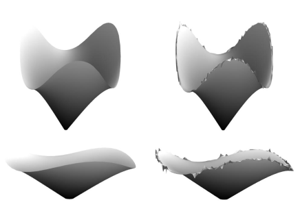
Fig.  5: The bluebell phase, obtained by numerical solution of (11) for two flexible tissues: $a=0.07$ (first row) and $a=0.14$ (second row). Figures on the right show appearance of buckling instabilities at the edge with growth.

The non-existence of real solutions of the eikonal equation at late stages is a direct consequence of the presence of finite bending scale, on which the tissue is locally flat. As it was mentioned above and is shown in the Fig.5, low values of $a$ lead to elongated conical regime. Since $a$ stands for the scale on which the circumference length of the tissue doubles, in the $a\to 0$ limit the real solution exists everywhere inside the disk, but it is everywhere flat (conical). Hopefully, the analytic continuation allows one to investigate buckling for negative values of $n^{2}(u,v)=J^{2}(u,v)-1$ by taking the absolute value of the solution, at least not far away from the zero-curve $\Gamma$. In this regime buckling instabilities on the circumference of the bluebell arise. In the Fig.6 we show proliferation of buckling near the critical point. First, the evolution of buckling instabilities at the edge can be understood as a subsequent doubling of peaks and saddles along the direction of growth. Then some hierarchy in peaks size is seen. We note, that this hierarchical organization is a natural result due to the theoretic-number properties of the Dedekind $\eta$-function. Though it is known, that in real plants and flowers buckling instabilities do not proliferate profoundly, since the division process is getting limited at late stages of growth, the formal continuation of the eikonal equation beyond $\Gamma$ predicts a self-similar buckling profile at the circumference of growing tissues.

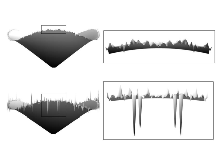
Fig.  6: Development of buckling instabilities at the edge of flower for rigidity parameter $a=0.14$. The right figures show hierarchical organization of the flower’s circumference in detail.

Now we pay attention to the directed growth above the half-plane domain. Here we solve the equation (12) with the Dirichlet boundary conditions, set along the line $t=1$, and the tissue is growing towards the boundary $t=0$ in the upper halfplane $\textrm{Im}\,r>0$. At low stages of growth the solution is flat until the first buckling mode appear, Fig.7. The subsequent growth is described by taking the absolute value of the solution, since no real solution exists anymore. As in the former case, the behavior is controlled by the value of $a$.

When the growth approaches the boundary, the edge of the tissue becomes more and more wrinkled. Emergence of new buckling modes is the consequence of the Dedekind $\eta$-function properties: doubling of parental peaks at the course of growth. Under the energetic approach for a leaf, very similar fractal structures can be inferred from the interplay between stretching and bending energies in the limit of extremely thin membranes: while the cell density (and the corresponding strain, $\sigma$) on the periphery increases, the newly generating wavelengths decrease, $\lambda\sim\sigma^{-1/4}$, ⁹.

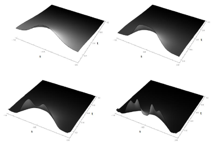
Fig.  7: Numerical solutions of (12) for the directed growth. Figures show enhancing of buckling at the edge.

Increasing the size $a$ of the elementary flat triangle domain, we figure out, that for some critical value, $a_{cr}$, the starting plateau of the corresponding Jacobian crosses the zero level and becomes negative. Our model implies no solutions for such stiff tissues. This limitation is quite natural since we do not consider in-plane deformations of the tissue. In reality, for $a>a_{cr}$ the tissue is so stiff, that it turns beneficial to be squeezed in-plane rather than to buckle out. One may conjecture that $a$ is the analogue of the Young modulus, $E$, that is known to regulate the rigidity of the tissue in the energetic approach, along with the thickness, $h$, and the Poisson modulus, $\mu$, in their certain combination, known as bending stiffness, $D=\frac{Eh^{3}}{12(1-\mu^{2})}$.

It is worth mentioning that at first stages of growth, until the instabilities at the circumference have not yet appeared, at certain angles (triangle-like cells) the surface bends similar to the Beltrami’s pseudosphere, that has a constant negative curvature at every point of the surface, compare Fig.5 and Fig.8. The similarity is even more striking for very low $a$, when the triangulating parameter is fairly small. It is known that the pseudosphere locally realizes the Lobachevsky geometry and can be isometrically mapped onto the finite part of the half-plane or of the Poincaré disk, Fig.8a-b. According to the Hilbert theorem, ³², no full isometric embedding of the Poincaré disk into the 3D space exists. Thus, in order to organize itself in the 3D space, the plant grows by the cascades of pseudospheres, resembling peaks and saddles, that is an alternative view on essence of buckling.

Interestingly, some flowers, such as calla lilies, initially grow psuedospherically, but then crack at some stage of growth and start twisting around in a helix. Apparently, this is another route of dynamic organization of non-Euclidean isometry in the Euclidean space. The Dini’s surface, Fig.8c is known in differential geometry as a surface of constant negative curvature and, in comparison with the Beltrami’s pseudosphere, is infinite. The problem of sudden cracking of the lilies seems to be purely biological, but as soon as the crack appeared, the flower may relief the stresses caused by subsequent differential growth through twisting its petals in the Dini’s fashion.

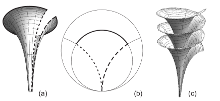
Fig.  8: (a)-(b) Pseudosphere and correspondence of boundaries on the Poincaré disc; (c) Dini surface.

Turn now to the eikonal interpretation of buckling. For the sake of simplicity, we will proceed here in the cartesian coordinates. Seeking the solution of (3) and (12) in the implicit form $H(\mathbf{x})\equiv H(x^{0},x^{1},x^{2})=H^{0}$ with $x^{0}=if$, $x^{1}=u$, $x^{2}=v$, we can rewrite (12) as:

$$g^{ij}\frac{\partial H(\mathbf{x})}{\partial x^{i}}\frac{\partial H(\mathbf{x})}{\partial x^{j}}=0;\quad g^{ik}=\left(\begin{matrix}n^{2}&0&0\\ 0&1&0\\ 0&0&1\end{matrix}\right)$$ (19)

Eq.(19) reveals the relativistic nature of the eikonal equation ²¹ and describes the propagation of light in a (2+1)D space-time in the gravitational field with induced metrics $g$ defined by the metric tensor $g^{ik}$, where $n\equiv n(x^{1},x^{2})$, speed of light put $c=1$. Having $g$, one can reconstruct geodesics that define the paths of the light propagation in our space-time. The parameterized geodesics family, $x^{\lambda}(\tau)$, where $\lambda=0,1,2$, can be found from the equation:

$$\frac{d^{2}x^{\lambda}}{d\tau^{2}}+\Gamma^{\lambda}_{ij}\frac{dx^{i}}{d\tau}\frac{dx^{j}}{d\tau}=0$$ (20)

where

$$\Gamma^{i}_{kl}=\frac{1}{2}g^{im}\left(\frac{\partial g_{mk}}{\partial x^{l}}+\frac{\partial g_{ml}}{\partial x^{k}}-\frac{\partial g_{kl}}{\partial x^{m}}\right)$$ (21)

are Christoffel symbols and $g_{ij}$ is the covariant form of the metrics ($g_{ij}g^{jk}=\delta^{k}_{i}$). Calculating the symbols for the specific metrics (19), we end up with the set of equations for the geodesics in a parametric form:

$$\left\{\begin{array}[]{l}\displaystyle u_{\tau\tau}-\frac{1}{n^{3}}\frac{\partial n}{\partial u}f_{\tau}^{2}=0,\vskip 6.0pt plus 2.0pt minus 2.0pt\\ \displaystyle v_{\tau\tau}-\frac{1}{n^{3}}\frac{\partial n}{\partial v}f_{\tau}^{2}=0,\vskip 6.0pt plus 2.0pt minus 2.0pt\\ \displaystyle f_{\tau\tau}-\frac{2}{n}\frac{dn}{d\tau}f_{\tau}=0\end{array}\right.$$ (22)

From the first two lines of (22), one gets $\frac{u_{\tau\tau}}{v_{\tau\tau}}=\frac{\partial n}{\partial u}\left(\frac{\partial n}{\partial v}\right)^{-1}$. Note, that the same relation follows directly from (2), if the planar domain is parameterized by the same coordinates $\mathbf{x}=\mathbf{x}(u,v)$. Thus, one may conclude, that the projections of the geodesics from the (2+1)D space-time onto the $(uv)$-plane coincide with light trajectories in the flat domain with refraction coefficient $n(u,v)$.

4 Conclusion and conjectures

In this paper we discussed the optimal buckling profile formation of growing two-dimensional tissue evoked by the exponential cell division from the point-like source and from the linear segment. Such processes imply excess material generation enforcing the tissue to wrinkle as it approaches the domain boundary. Resulting optimal hyperbolic surface is described by the eikonal equation for the two-dimensional profile, and allows for simple geometric optics analogy. It is shown that the surface height above the domain mimics the eikonal (action) surface of a particle moving in the 2D media with certain refraction index, $n$, which, in turn, is linked to microscopic rules of elementary cell division and symmetry of the plant. The projected geodesics of this ”minimal” optimal surface coincide with Fermat paths in the 2D media, which is the intrinsic feature of the eikonal equation. This result suggests an idea to treat the growth process itself as a propagation of the wavefronts in the media with certain metrics.

We have derived the metrics of the growing plant’s surface from microscopic rules of cells division and have shown that the solution of the eikonal equation describes buckling of tissues of different rigidities. Our results, being purely geometric, rhyme well with a number of energetic approaches to buckling of thin membranes, where the stiffness is controlled by the effective bending rigidity. We show that presence of a finite scale on which the tissue remains flat, results in negatively curved growing surfaces and the eikonal equation implies absence of real solution at late stages of the growth. Though, an analytical continuation can be constructed and erratic self-similar patterns along the circumference can be obtained. In reality high energetic costs for the profound cell division after bifurcation point would prohibit infinite growth and intense buckling.

Recall, that the right-hand side of the eikonal equation mimics the squared refraction index, (13), if buckling is interpreted as wavefront propagation in geometric optics. At length of our work it was pointed out, that for the differential growth problem, negative square of refraction index leads to complex solution for $f$. Does complex solution have any physical meaning for growth? We can provide the following speculation. The complex solution appears for the late stages of growth when the finite bending scale of the tissue prohibits formation of very low-wavelength buckling modes. Since in this regime the tissue would experience in-plane deformations, one may improve the geometric model by letting branches to accumulate the ”potential energy”. Thereby, the analogy between optics and differential growth can be advanced by noting that the negative squared refraction index means absorbtion properties of the media. The propagating wavefront of a moving particle, dissipates the energy in areas where the refraction index is complex-valued. In the differential growth the proliferation of buckling modes may be limited by the energy losses at branches, that would suppress buckling.

The challenging question concerns the possibility to extend our approach to the growth of three-dimensional objects, for example, of a ball that size $R$ grows faster than $R^{2}$. In this case, the redundant material can provoke the surface instabilities. We conjecture that some analogy between the boundary growth and optic wavefronts survives in this case as well.

Authors are grateful to M. Tamm, A. Grosberg, M. Lenz, L. Mirny and L. Truskinovsly for valuable discussions of various aspects of the work and to A. Orlov for invaluable help in numerical solution of the eikonal equation. The work is partially supported by the IRSES DIONICOS and RFBR 16-02-00252A grants.

Appendix: Conformal transformation of the flat triangle to the Poincare domain

The conformal mapping $z(w)$ of the flat equilateral triangle $ABC$ located in $z$ onto the zero-angled triangle $ABC$ in $w$, used in the derivation of (14), is constructed in four sequential steps, shown in the Fig.9.

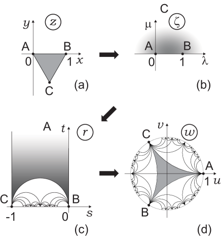
Fig.  9: Conformal mapping $z(w)$ is realized as a composition of three mappings: $z(\zeta)$ [(a)–(b)], $\zeta(r)$ [(b)–(c)], and $r(w)$ [(c)–(d)]. Finally we have $z(\zeta(r(w)))$.

First, we map the triangle $ABC$ in $z$ onto the upper half-plane $\zeta$ of auxiliary complex plane $\zeta$ with three branching points at 0, 1 and $\infty$ – see the Fig.9a-b. This mapping is realized by the function $z(\zeta)$:

$$z(\zeta)=\frac{\Gamma(\frac{2}{3})}{\Gamma^{2}(\frac{1}{3})}\int_{0}^{\zeta}\frac{d\xi}{\xi^{2/3}(1-\xi)^{2/3}}$$ (23)

with the following coincidence of branching points:

$$\left\{\begin{array}[]{lcl}A(z=0)&\leftrightarrow&A(\zeta=0)\vskip 6.0pt plus 2.0pt minus 2.0pt\\ B(z=1)&\leftrightarrow&B(\zeta=1)\vskip 6.0pt plus 2.0pt minus 2.0pt\\ C(z=e^{-i\frac{\pi}{3}})&\leftrightarrow&C(\zeta=\infty)\end{array}\right.$$ (24)

Second step consists in mapping the auxiliary upper half-plane $\Im\zeta>0$ onto the circular triangle $ABC$ with angles $\{\alpha,\alpha,0\}$ – the fundamental domain of the Hecke group ²³ in $r$, where we are intersted in the specific case $\{\alpha,\alpha,0\}=\{0,0,0\}$ – see Fig.9b-c. This mapping is realized by the function $\zeta(r)$, constructed as follows ²⁶. Let $\zeta(r)$ be the inverse function of $r(\zeta)$ written as a quotient

$$r(\zeta)=\frac{\phi_{1}(\zeta)}{\phi_{2}(\zeta)}$$ (25)

where $\phi_{1,2}(\zeta)$ are the fundamental solutions of the 2nd order differential equation of Picard-Fuchs type:

$$\zeta(\zeta-1)\phi^{\prime\prime}(\zeta)+\big{(}(a+b+1)\zeta-c\big{)}\phi^{\prime}(\zeta)\\ +ab\phi(\zeta)=0$$ (26)

Following ^{27, 26}, the function $r(\zeta)$ conformally maps the generic circular triangle with angles $\{\alpha_{0}=\pi|c-1|,\alpha_{1}=\pi|a+b-c|,\alpha_{\infty}=\pi|a-b|\}$ in the upper halfplane of $w$ onto the upper halfplane of $\zeta$. Choosing $\alpha_{\infty}=0$ and $\alpha_{0}=\alpha_{1}=\alpha$, we can express the parameters $(a,b,c)$ of the equation (26) in terms of $\alpha$, taking into account that the triangle $ABC$ in the Fig.9c is parameterized as follows $\{\alpha_{0},\alpha_{1},\alpha_{\infty}\}=\{\alpha,\alpha,0\}$ with $a=b=\frac{\alpha}{\pi}+\frac{1}{2},c=\frac{\alpha}{\pi}+1$. This leads us to the following particular form of equation (26)

$$\zeta(\zeta-1)\phi^{\prime\prime}(\zeta)+\Big{(}\frac{\alpha}{\pi}+1\Big{)}\big{(}2\zeta-1\big{)}\phi^{\prime}(\zeta)\\ +\Big{(}\frac{\alpha}{\pi}+\frac{1}{2}\Big{)}^{2}\phi(\zeta)=0$$ (27)

where $\alpha=\frac{\pi}{m}$ and $m=3,4,...\infty$. For $\alpha=0$ Eq.(27) takes an especially simple form, known as Legendre hypergeometric equation ^{28, 29}. The pair of possible fundamental solutions of Legendre equation are

$$\begin{array}[]{l}\phi_{1}(\zeta)=F\big{(}\frac{1}{2},\frac{1}{2},1,\zeta\big{)}\vskip 6.0pt plus 2.0pt minus 2.0pt\\ \phi_{2}(\zeta)=iF\big{(}\frac{1}{2},\frac{1}{2},1,1-\zeta\big{)}\end{array}$$ (28)

where $F(...)$ is the hypergeometric function. From (25) and (28) we get $r(\zeta)=\frac{\phi_{1}(\zeta)}{\phi_{2}(\zeta)}$. The inverse function $\zeta(r)$ is the so-called modular function, $k^{2}(r)$ (see ^{28, 29, jacobi2} for details). Thus,

$$\zeta(r)\equiv k^{2}(r)=\frac{\theta_{2}^{4}(0,e^{i\pi r})}{\theta_{3}^{4}(0,e^{i\pi r})}$$ (29)

where $\theta_{2}$ and $\theta_{3}$ are the elliptic Jacobi $\theta$-functions ^{jacobi2, 30},

$$\begin{array}[]{l}\displaystyle\theta_{2}\left(\chi,e^{i\pi w}\right)=2e^{i{\pi\over 4}r}\sum_{n=0}^{\infty}e^{i\pi rn(n+1)}\cos(2n+1)\chi\vskip 6.0pt plus 2.0pt minus 2.0pt\\ \displaystyle\theta_{3}\left(\chi,e^{i\pi r}\right)=1+2\sum_{n=1}^{\infty}e^{i\pi rn^{2}}\cos 2n\chi\end{array}$$ (30)

and the correspondence of branching points in the mapping $\zeta(r)$ is as follows

$$\left\{\begin{array}[]{lcl}A(\zeta=0)&\leftrightarrow&A(r=\infty)\vskip 6.0pt plus 2.0pt minus 2.0pt\\ B(\zeta=1)&\leftrightarrow&B(r=0)\vskip 6.0pt plus 2.0pt minus 2.0pt\\ C(\zeta=\infty)&\leftrightarrow&C(r=-1)\end{array}\right.$$ (31)

Third step, realized via the function $r(w)$, consists in mapping the zero-angled triangle $ABC$ in $r$ into the symmetric triangle $ABC$ located in the unit disc $w$ – see Fig.9c-d. The explicit form of the function $r(w)$ is

$$r(w)=e^{-i\pi/3}\frac{e^{2i\pi/3}-w}{1-w}-1$$ (32)

with the following correspondence between branching points:

$$\left\{\begin{array}[]{lcl}A(r=\infty)&\leftrightarrow&A(w=1)\vskip 6.0pt plus 2.0pt minus 2.0pt\\ B(r=0)&\leftrightarrow&B(w=e^{-2\pi i/3})\vskip 6.0pt plus 2.0pt minus 2.0pt\\ C(r=-1)&\leftrightarrow&C(w=e^{2\pi i/3})\end{array}\right.$$ (33)

Collecting (23), (29), and (32) we arrive at the following expression for the derivative of composite function,

$$z^{\prime}(\zeta(r(w)))=z^{\prime}(\zeta)\,\zeta^{\prime}(r)\,r^{\prime}(w)$$ (34)

where ^′ stands for the derivative. We have explicitly:

$$z^{\prime}(\zeta)=\frac{\Gamma(\frac{2}{3})}{\Gamma^{2}(\frac{1}{3})}\,\frac{\theta_{3}^{16/3}(0,\zeta)}{\theta_{2}^{8/3}(0,\zeta)\;\theta_{0}^{8/3}(0,\zeta)}$$

and

$$\zeta^{\prime}(r)|=i\pi\frac{\theta_{2}^{4}\;\theta_{0}^{4}}{\theta_{3}^{4}};\qquad i\frac{\pi}{4}\theta_{0}^{4}=\frac{d}{d\zeta}\ln\left(\frac{\theta_{2}}{\theta_{3}}\right)$$

The identity

$$\theta^{\prime}_{1}(0,e^{i\pi\zeta})\equiv\left.\frac{d\theta_{1}(\chi,e^{i\pi\zeta})}{d\chi}\right|_{\chi=0}\\ =\pi\theta_{0}(\chi,e^{i\pi\zeta})\,\theta_{2}(\chi,e^{i\pi\zeta})\,\theta_{3}(\chi,e^{i\pi\zeta})$$ (35)

enables us to write

$$\left|z^{\prime}(r)\right|^{2}=h^{2}\left|\theta^{\prime}_{1}\left(0,e^{i\pi r}\right)\right|^{8/3}$$ (36)

where $h=\left(\frac{16}{\pi}\right)^{1/3}\frac{\Gamma(\frac{2}{3})}{\Gamma^{2}(\frac{1}{3})}$, and

$$\theta_{1}(\chi,e^{i\pi r})=2e^{i\frac{\pi}{4}r}\sum_{n=0}^{\infty}(-1)^{n}e^{i\pi n(n+1)r}\sin(2n+1)\chi\vskip 6.0pt plus 2.0pt minus 2.0pt\\$$ (37)

Differentiating (32), we get

$$r^{\prime}(w)=\frac{i\sqrt{3}}{(1-w)^{2}}$$

and using this expression, we obtain the final form of the Jacobian of the composite conformal transformation $J(z(\zeta(r(w))))$:

$$J(z(w))=|z^{\prime}(w)|^{2}=3h^{2}\frac{|\eta(r(w))|^{8}}{|1-w|^{4}}$$ (38)

where

$$\eta(r)=\big{(}\theta_{1}^{\prime}(0,e^{i\pi r})\big{)}^{1/3}$$

is the Dedekind $\eta$-function (see (15)), and the function $r(w)$ is defined in (32).

References

- 1 M. A. R. Koehl, W.K. Silk, H. Liang, L. Mahadevan, Integrative and Comparative Biology, 2008, 48, 834.
- 2 D.W. Henderson, D. Taimina, The Mathematical Intelligencer, 2001, 23, 17.
- 3 S. Nechaev, R. Voituriez, Journal of Physics A: Math. Gen., 2001, 34, 11069.
- 4 S. Nechaev, O. Vasilyev, Journal of Physics A: Math. Gen., 2004, 37, 3783.
- 5 V. Borrelli, S. Jabrane, F, Lazarus, and B. Thibert, Proceedings of the National Academy of Sciences, 2012, 109, 7218.
- 6 M. Lewicka, L. Mahadevan, M.R. Pakzad, Proceedings of Royal Society A, 2011, 467, 402.
- 7 J. Gemmer, S.C. Venkataramani, Soft Matter, 2013, 9, 8151.
- 8 J. W. S. Rayleigh, The theory of sound, Dover, New York, 1945.
- 9 E. Cerda, K. Ravi-Chandar, L. Mahadevan, Nature, 2002, 419, 579.
- 10 E. Efrati, E. Sharon, R. Kupferman, 2009, Journal of the Mechanics and Physics of Solids, 57, 762.
- 11 Nath, U., Crawford, B. C., Carpenter, R., Coen, E., Science, 2003, 299, 1404.
- 12 E. Sharon, B. Roman, M. Marder, G.-S. Shin, and H. L. Swinney, Nature, 2002, 419, 579.
- 13 E. Sharon, B. Roman, and H. L. Swinney, Physical Review E, 2007, 75, 046211.
- 14 H. Liang, L. Mahadevan, Proceedings of the National Academy of Sciences, 2009, 106, 22049.
- 15 B. Audoly, A. Boudaoud, Physical Review Letters, 2003, 91, 086105.
- 16 M. Marder et al., Europhysics Letters, 2003, 62, 498.
- 17 M. Marder, N. Papanicolaou, Journal of Statistical Physics, 2006, 125, 1065.
- 18 A. Goriely, M. Ben Amar, Phisical Review Letters, 2005, 94, 198103.
- 19 N. Stoop et al., Physical Review Letters, 2010, 105, 068101.
- 20 L. S. Levitov, Europhysics Letters, 1991, 14, 533.
- 21 L.D. Landau, E.M. Lifshitz, Course of theoretical physics, Theory of elasticity, Pergamon Press, Oxford, 1986.
- 22 K. Chandrassekharan, Elliptic Functions, Springer, Berlin, 1985.
- 23 Li-Chien Shen, The Ramanujan Journal, 2016, 39, 609.
- 24 F. Klein, Jahresbericht der Deutschen Mathematiker-Vereinigung, 1890, 1, 35.
- 25 Y.B. Rumer, Uspekhi Matematicheskikh Nauk, 1953, 8, 55.
- 26 W. Koppenfels, F. Stallman, Praxis der konformen Abbildung, Springer, Berlin, 1959.
- 27 C. Carathéodory, Theory of functions, vol. II, Chelsea Pub. Company, New York, 1954.
- 28 V.V. Golubev, Lectures on the analytic theory of differential equations, Gostekhizdat, Moscow, 1950
- 29 E. Hille, Ordinary differential equations in the complex plane, J. Willey & Sons, New York, 1976.
- 30 D. Mumford, C. Musili, Tata lectures on theta II, Springer, Berlin, 2007.
- 31 M.H. Amsler, Mathematische Annalen, 1955, 130, 234.
- 32 D. Hilbert, Transactions of the American Mathematical Society, 1901, 2, 87.
- 33 G.M. Fihtengolc, Kurs Diferencialnovo i Integralnovo Iscislenia I, Nauka, Moscow, 1966.